
Markov and mixed models with applications -...
181
General rights Copyright and moral rights for the publications made accessible in the public portal are retained by the authors and/or other copyright owners and it is a condition of accessing publications that users recognise and abide by the legal requirements associated with these rights. Users may download and print one copy of any publication from the public portal for the purpose of private study or research. You may not further distribute the material or use it for any profit-making activity or commercial gain You may freely distribute the URL identifying the publication in the public portal If you believe that this document breaches copyright please contact us providing details, and we will remove access to the work immediately and investigate your claim. Downloaded from orbit.dtu.dk on: Jun 03, 2019 Markov and mixed models with applications Mortensen, Stig Bousgaard Publication date: 2010 Document Version Publisher's PDF, also known as Version of record Link back to DTU Orbit Citation (APA): Mortensen, S. B. (2010). Markov and mixed models with applications. Kgs. Lyngby, Denmark: Technical University of Denmark (DTU). IMM-PHD-2009-220
Transcript of Markov and mixed models with applications -...

General rights Copyright and moral rights for the publications made accessible in the public portal are retained by the authors and/or other copyright owners and it is a condition of accessing publications that users recognise and abide by the legal requirements associated with these rights.
Users may download and print one copy of any publication from the public portal for the purpose of private study or research.
You may not further distribute the material or use it for any profit-making activity or commercial gain
You may freely distribute the URL identifying the publication in the public portal If you believe that this document breaches copyright please contact us providing details, and we will remove access to the work immediately and investigate your claim.
Downloaded from orbit.dtu.dk on: Jun 03, 2019
Markov and mixed models with applications
Mortensen, Stig Bousgaard
Publication date:2010
Document VersionPublisher's PDF, also known as Version of record
Link back to DTU Orbit
Citation (APA):Mortensen, S. B. (2010). Markov and mixed models with applications. Kgs. Lyngby, Denmark: TechnicalUniversity of Denmark (DTU). IMM-PHD-2009-220
Markov and mixed models
with applications
Stig Bousgaard Mortensen
Kongens Lyngby 2009IMM-PHD-2009-220

Technical University of DenmarkInformatics and Mathematical ModellingBuilding 321, DK-2800 Kongens Lyngby, DenmarkPhone +45 45253351, Fax +45 [email protected]
IMM-PHD: ISSN 0909-3192
Preface
This thesis was submitted at the Technical University of Denmark (DTU), de-partment of Informatics and Mathematical Modelling (IMM) in partial fulfil-ment of the requirement for acquiring the PhD degree in engineering.
The topic of the thesis is application of Markov and mixed models to theanalysis of sleep EEG data and pharmacokinetic and pharmacodynamic modelsin general. The thesis consists of a summary report and five research paperswritten during the PhD study. Four are submitted to or published in interna-tional journals and one is published as a research report at DTU/IMM.
I would like to thank my supervisors Henrik Madsen from DTU/IMM andPhilip Hougaard from H. Lundbeck A/S for their excellent support and ideasduring the project. Also, I wish to thank my colleagues at both DTU/IMMand H. Lundbeck for valuable discussions and for making it a enjoyable timeduring the project and also in particular my fellow PhD students Anna HelgaJonsdottır, Søren Klim and Rune H. B. Christensen for their collaboration indifferent projects.
Lyngby, September 2009
Stig Bousgaard Mortensen

ii Preface

Abstract
This thesis deals with mathematical and statistical models with focus on appli-cations in pharmacokinetic and pharmacodynamic (PK/PD) modelling. Thesemodels are today an important aspect of the drug development in the pharma-ceutical industry and continued research in statistical methodology within theseareas are thus important.
PK models are concerned with describing the concentration profile of a drugin both humans and animals after drug intake whereas PD models are used todescribe the effect of a drug in relation to the drug concentration. PK models foran individual are usually described as a deterministic mean value using ordinarydifferential equations to which a random error is added. This thesis exploresmethods based on stochastic differential equations (SDEs) to extend the modelsto more adequately describe both true random biological variations and alsovariations due to unknown or uncontrollable factors in an individual. Modellingusing SDEs also provides new tools for estimation of unknown inputs to a systemand is illustrated with an application to estimation of insulin secretion rates indiabetic patients.
Models for the effect of a drug is a broader area since drugs may affectthe individual in almost any thinkable way. This project focuses on measuringthe effects on sleep in both humans and animals. The sleep process is usuallyanalyzed by categorizing small time segments into a number of sleep states andthis can be modelled using a Markov process. For this purpose new methods fornon-parametric estimation of Markov processes are proposed to give a detaileddescription of the sleep process during the night.
Statistically the Markov models considered for sleep states are closely relatedto the PK models based on SDEs as both models share the Markov property.When the models are applied to clinical data there will often be a large variationbetween individuals and this can be included in both types of models usingthe mixed modelling approach. Estimation in these models is discussed withemphasis on data with a more complex grouping structure.

iv Abstract
Resume
(Abstract in Danish.)
Denne afhandling beskæftiger sig med matematiske og statistiske modeller medfokus pa applikationer indenfor farmakokinetisk og farmakodynamisk (PK/PD)modellering. Disse modeller udgør i dag et vigtigt aspekt af udvikling af lægemi-dler i den farmaceutiske industri og fortsat forskning i statistiske metoder indenfor disse omrader er derfor vigtig.
PK modeller beskriver koncentrationsprofilen af medicin i bade menneskerog dyr efter indtagelse af et lægemiddel hvorimod PD modeller bruges til atbeskrive virkningen af et lægemiddel i relation til koncentrationsprofilen. Of-test bliver PK modeller for et individ beskrevet deterministisk ved brug af or-dinære differentialligninger. Denne afhandling undersøger metoder baseret pastokastiske differentialligninger (SDEer) der gør det muligt udvide disse modellertil at beskrive variation fra bade tilfældige biologiske effekter og ogsa variationerfra ukendte eller ukontrollerbare faktorer i et individ. Modellering ved hjælp afSDEer giver ogsa nye metoder til estimering af ukendt input til et system, ogdette er illustreret her med en anvendelse til estimering af raten for insulinpro-duktion i diabetespatienter.
Modeller for virkningen af lægemidler er et bredere omrade da de kan pavirkedet enkelte individ pa et næsten ubegrænset antal mader. Dette projekt fokusererpa at male effekten pa søvn i bade mennesker og dyr. Søvnstrukturen blivernormalt analyseret ved at kategorisere sma tidssegmenter i et antal søvnstadier,og dette kan modelleres ved brug af en Markov proces. Til dette formal er derudviklet nye ikke-parametriske metoder til estimering af Markov processer forat kunne give en detaljeret beskrivelse af søvnstrukturen i løbet af natten.
Statistisk er Markov modeller for søvnstadier tæt relateret til PK modellerbaseret pa SDEer da de begge deler Markov egenskaben. Nar disse modelleranvendes til kliniske data, vil der ofte være en stor variation mellem enkeltper-soner og denne kan beskrives i begge typer af modeller ved at anvende sakaldtemixede modeller. Estimation i disse modeller bliver behandlet med vægt padata med en mere kompleks grupperingsstruktur.
List of publications
The thesis is based on the following five scientific research papers,
A Mortensen SB, Klim S, Dammann B, Kristensen NR, Madsen H, Over-gaard RV. A Matlab Framework for Estimation of NLME Models usingStochastic Differential Equations: Applications for estimation of insulinsecretion rates. Journal of Pharmacokinetics and Pharmacodynamics 34,pp. 623-42 (2007).
B Mortensen SB, Jonsdottır AH, Klim S, and Madsen H. Introduction toPK/PD modelling with focus on PK and stochastic differential equations.IMM-Technical Report-2008-16 (2008).
C Klim S, Mortensen SB, Kristensen NR, Overgaard RV and Madsen H.Population stochastic modelling (PSM) - An R package for mixed-effectsmodels based on stochastic differential equations. Computer Methods andPrograms in Biomedicine 94, pp. 279-289 (2009).
D Mortensen SB, Madsen H, and Hougaard P. Local Estimation of a Dis-cretely Observed Continuous Time Inhomogeneous Markov Jump Process.Submitted to Statistical Modelling (2009).
E Mortensen SB and Christensen RHB. Flexible Estimation of nonlinearmixed models via Laplace’s approximation. Submitted to Journal of theAmerican Statistical Association (2009).
vi List of publications
Below is a list of other publications also prepared during the PhD project. Thescientific content is covered in papers A, B and C and they will thus not beadressed in this thesis.
• Klim S, Mortensen SB, Madsen H, Overgaard RV and Kristensen NR.“Stochastic PK/PD modelling”. Poster for Seminaire Europeen de Statis-tique, Cartagena, Spain (2007).
• Mortensen SB og Klim S. “Population Stochastic Modelling (PSM): Modeldefinition, description and examples”. Package vignette for the R packagePSM. Url: http://www.imm.dtu.dk/psm/doc/PSM.pdf (2008).
• Mortensen SB og Klim S. “Package: PSM”. User manual for the R packagePSM. Url: http://www.imm.dtu.dk/psm/PSM-help.pdf (2008).
• Klim S, Mortensen SB and Madsen H. Linear Mixed Effects models basedon Stochastic Differential Equations in R. Poster for Annual Meeting ofthe Population Approach Group in Europe, Marseille, France (2008).
• Jonsdottır AH, Klim S, Mortensen SB, and Madsen H. Chapter “Mate-matik i medicinudvikling” (eng.: Mathematics in drug development) forthe book “Matematiske horisonter” (eng.: Mathematical horizons), ISBN978-87-643-0453-4 (2009).
• Nielsen HB and Mortensen SB. “Package: ucminf” User manual for forthe R package ucminf for quasi-Newton optimization. Url: http://cran.r-project.org/web/packages/ucminf/
In collaboration with other researchers the following papers were also preparedduring the PhD project. They are based on earlier work and hence will not beadressed here.
• Yoon CH, Bodvarsson B, Klim S, Mørkebjerg M, Mortensen SB, Chen J,Maclaren JR, Luther PK, Squire JM, Bones PJ, Millane RP. Determina-tion of Myosin Filament Orientations in Electron Micrographs of MuscleCross Sections. IEEE Trans. Image Process., 18(4), 831-839 (2009).
• Bodvarsson B, Klim S, Mørkebjerg M, Mortensen SB, Yoon CH, ChenJ, Maclaren JR, Luther PK, Squire JM, Bones PJ and Millane RP. Amorphological image processing method for locating myosin filaments inmuscle electron micrographs. Image and Vision Computing 26, 1073-1080(2008).
Contents
Preface i
Abstract iii
List of publications v
1 Introduction 1
2 Mixed models 5
2.1 Parameter estimation . . . . . . . . . . . . . . . . . . . . . . . . 62.2 Evaluation of the marginal likelihood . . . . . . . . . . . . . . . . 62.3 Multivariate Laplace approximation . . . . . . . . . . . . . . . . 92.4 The nonlinear mixed model . . . . . . . . . . . . . . . . . . . . . 11
3 Inhomogeneous Markov processes 15
3.1 Sleep EEG . . . . . . . . . . . . . . . . . . . . . . . . . . . . . . 163.2 Model definition . . . . . . . . . . . . . . . . . . . . . . . . . . . 233.3 Non-parametric estimation . . . . . . . . . . . . . . . . . . . . . 263.4 Parametric estimation . . . . . . . . . . . . . . . . . . . . . . . . 333.5 Discussion . . . . . . . . . . . . . . . . . . . . . . . . . . . . . . . 36
4 Stochastic differential equations 39
4.1 Brownian motion . . . . . . . . . . . . . . . . . . . . . . . . . . . 404.2 Ito integrals . . . . . . . . . . . . . . . . . . . . . . . . . . . . . . 40

viii CONTENTS
4.3 Filtering problem . . . . . . . . . . . . . . . . . . . . . . . . . . . 424.4 Likelihood estimation . . . . . . . . . . . . . . . . . . . . . . . . 454.5 Mixed models with SDEs . . . . . . . . . . . . . . . . . . . . . . 464.6 Applications of SDE based models . . . . . . . . . . . . . . . . . 47
5 Conclusion 51
A Paper A 59
B Paper B 81
C Paper C 121
D Paper D 133
E Paper E 149

Chapter 1
Introduction
The drug development process in the pharmaceutical industry today generatesincreasing amounts of data and this requires ongoing development and refine-ment of the methods applied for the analysis. The present project exploresmethods based on Markov and nonlinear mixed effects models with applicationsmainly within pharmacokinetics and pharmacodynamics (PK/PD).
Nonlinear mixed models (NLMMs) are used as a standard tool today forwhat is often referred to as population PK/PD modelling. Mixed models aremodels with both fixed and random effects and can in many cases effectivelydescribe both the common structure of a response and the random variationbetween e.g. a number of individuals in the data. This thesis extends the classof models that can easily be fitted in this framework. For NLMMs the maximumlikelihood estimation involves an integral of dimension equal to the number ofrandom effects in the model. In cases where random effects only occur for onelevel of grouping in the data (e.g. individuals) or if random effects are nested(e.g. separate groups of individuals are observed at different study centers)the dimensionality of the integration problem can be significantly reduced usingstandard methods. This type of model structure has almost solely been the focusof statistical software for estimation of NLMMs, which goes back to the firstsoftware tool NONMEM (Beal and Sheiner, 2004) which was initially introducedaround 1980 (Beal and Sheiner, 1980). Situations with crossed random effectswhere e.g. some individuals are observed at more than one study center requiresan evaluation of the full dimensional integral. In Chapter 2 it will be describedhow this problem can be handled using the multivariate Laplace approximation.
2 Introduction
Pharmacokinetics and pharmacodynamics are in popular terms often de-scribed as “what the body does to the drug” and “what the drug does to thebody”, respectively. Research in these disciplines has a long history and todaythese disciplines constitute an important part of the drug development process.A general introduction to PK/PD is given in paper B and a more thoroughdescription can be found in e.g. Rowland and Tozer (1997) or (Gabrielsson andWeiner, 2006).
Pharmacodynamics is concerned with the effects of the drug. The effect ofa drug can e.g. be lowering of the blood pressure, in which case it is relativelystraight forward to measure, or it can be reducing pain, which is somewhat moredifficult to quantify. An example of a PD model for a pain reliever is illustratedin paper B. Here the effect is measured on a visual analogue scale and this islinked to a PK model to get a full PK/PD model for the drug.
A part of this project has been concerned with effect measures for sleepand in particular a measure of sleep related to time. This study was initiatedby a new drug candidate Gaboxadol which has been under development by H.Lundbeck. Studies have shown that Gaboxadol has sleep promoting effects thatdiffers from currently marketed sleep drugs.
Sleep is mainly studied using the electroencephalogram (EEG) which recordselectrical signals from the neurons in the brains by placing a number of electrodeson the scalp. The electrical signals are sampled at a high frequency of e.g.100 Hz which results in a raw EEG recording. This recording is traditionallytransformed into sleep stages, where each segment of data of usually either 10 or30 seconds (called the epoch length) is classified into sleep stages. For humansthere are six stages, namely wake, REM sleep and sleep stages 1 to 4. Thesesleep stages were defined by Rechtschaffen and Kales (1968) and has been usedas a gold standard ever since. For rodents similar analysis can be performed,but here it is usually only possible to classify 3 sleep stages, namely wake, deltasleep and paradoxical sleep where the two latter are related to sleep stages 3-4and REM sleep in humans, respectively.
Traditionally sleep has been evaluated by means of simple summaries liketime spent in each sleep stage, time to sleep onset and similar measures. Inorder to study the dynamics of changes of the sleep process over night in moredetail it is chosen to model the sequence of sleep stages as an inhomogeneousMarkov process. Estimation of changes in parameters of the inhomogeneousMarkov model is discussed in Chapter 3 where a method based on local kernelestimation is proposed for solving the estimation problem. It is further shownhow this can be used to estimate the pharmacodynamic effect of Gaboxadol.
Pharmacokinetics is the study of how a drug enters and circulates throughthe body and in general it describes where the drug is in the body as a functionof time. The dynamical description of the body as a system is obtained usinga compartmental model structure, where each compartment represents an area

3
of the body where the drug is contained and can be assumed to be evenly dis-tributed. Examples of potential compartments are the bloodstream, muscles,the stomach or peripheral tissue. The movement of the drug between the com-partments is traditionally described using ordinary differential equations andthus implicitly defines the body as a deterministic system without any randombiological variation. If such random biological variation is actually present orif some parts of the system is not adequately described this may result in se-rial correlation in the residuals between observations and model in a statisticalanalysis.
To appropriately model these phenomena is has been proposed to introducestochastic differential equations (SDEs) for the modelling. By using SDEs itis possible to include stochastic components in the model of a system to com-pensate for true biological variation or structural misspecification of the model.A part of this project has been concerned with the development of a softwaretool for estimation of the embedded parameters of a general nonlinear mixedmodel based on SDEs. This will be presented and discussed in more detail inChapter 4 and will also include applications of the modelling approach. Likefor the mixed model this work allows for using models that were previously toocomplex to be used.

4 Introduction

Chapter 2
Mixed models
Mixed models make up a general class of models for the analysis of groupeddata. A mixed model handles dependence between observations within groupsby assuming the existence of one or more unobserved latent variables for eachgroup of data. The unobserved latent variables are assumed to be random andhence referred to as random effects. A mixed model thereby consists of bothfixed model parameters θ and random effects b for modelling both the commonand group dependent structures in the data. Modelling using both fixed andrandom effects has coined the term mixed-effects models or in short just mixedmodels.
Random effects naturally enter the modelling when data is observed based ona number of experimental units that are taken from a larger population. In suchcases it is often found that e.g. individuals from a population are very similarbut exhibit a certain amount of variation that is most appropriately modelledas random. The distribution of the random effects thus represents the randomvariation in the populations that cannot otherwise be reasonably explained byfixed effects and covariates. In this way inference based on a mixed modelwhere the random effect distribution has been estimated along with the modelparameters will apply to the population as a whole and not only the individualsselected for the study. From an inferential point of view this is the main benefitachieved using a mixed modelling approach along with the possibility of judgingindividual covariates such as sex, weight and height.
There are no constraints on the assumed distribution for the random effects,but for a very wide range of applications they are assumed to have a Gaussian

6 Mixed models
distribution with mean zero such that
b ∼ N(0,Ψ).
The random effect distribution is thus completely described by its covariancematrix Ψ and this class of Gaussian mixed models will be the focus here.
2.1 Parameter estimation
Estimation in mixed models is based on maximum likelihood. The statisticaldescription of a mixed model is defined by a joint likelihood of the model pa-rameters and the unobserved random effects based on the joint density of (y, b).The joint likelihood is given as
L(θ,Ψ, b|y) = p(y, b|θ,Ψ) (2.1)= p(y|b,θ,Ψ)p(b|θ,Ψ) (2.2)= p1(y|b,θ)p2(b|Ψ) (2.3)
where (2.2) follows using Bayes’ theorem and (2.3) since p1(y|b) does not in-volve Ψ and p2(b|Ψ) likewise does not involve θ. The part of the model definingp1(y|b,θ) is sometimes referred to as the first stage model (with likelihood func-tion L1(b,θ|y)) and p2(b|Ψ) as the second stage model. To obtain the likelihoodfor the model parameters (θ,Ψ) the unobserved random effects are integratedout based on the assumed (here Gaussian) distribution. The likelihood functionfor estimating (θ,Ψ) is thus the marginal likelihood
LM (θ,Ψ|y) =∫
Rq
L(θ,Ψ, b|y)db (2.4)
where q is the number of random effects and θ and Ψ are the parameters tobe estimated. The likelihood function in (2.4) gives a very broad definition ofmixed models: the only requirement for using mixed modeling is to define ajoint likelihood function for the model of interest. In this way mixed modellingcan be applied to any likelihood based statistical modelling. Examples of appli-cations are linear mixed models (LMM) and nonlinear mixed models (NLMM)(regression type models, see e.g. Bates and Watts (1988)), generalized linearmixed models (McCulloch and Searle, 2001) but also models based on Markovchains and SDEs as will be the focus of Chapter 3 and 4.
2.2 Evaluation of the marginal likelihood
For many classes of statistical models the integral in (2.4) is intractable withno closed form solution available. An important exception to this is the widely

2.2 Evaluation of the marginal likelihood 7
used Gaussian linear mixed model where y = Xβ + Zb + ε, ε ∼ N(0,Σ), forwhich the marginal distribution of the observation y is given explicitly as amultivariate Gaussian distribution with mean Xβ and variance ZΨZT + Σ.For Gaussian nonlinear mixed models
y = f(β, b) + ε, ε ∼ N(0,Σ), (2.5)
where the model function f is nonlinear, it is no longer generally possible toderive an explicit marginal distribution. An exception to this is nonlinear mixedmodels which are nonlinear only in β but not b. Such a model can be re-writtenwith a first-order Taylor expansion around b = 0 as f(β, b) = f(β,0) +f ′b(β)bwhich is equivalent to a linear mixed model with Xβ = f(β,0) and Zb =f ′b(β)b. For a given set of parameters β the likelihood function can thus beevaluated based on the marginal multivariate Gaussian distribution as in thelinear mixed model. A clear distinction between nonlinear mixed models thatare either linear or nonlinear in the random effects is not always made, but isimportant from a computational viewpoint.
2.2.1 Likelihood approximations
For mixed models where there is no closed form solution to (2.4) it is necessaryto invoke some form of numerical approximation to be able to estimate themodel parameters. The complexity of this problem is mainly dependent thedimensionality of the integration problem which in turn is dependent on thegrouping structure in the data for the random effects. These structures includea single grouping, nested grouping, partially crossed and crossed random effects.
For problems with only one level of grouping the marginal likelihood can besimplified as
L(β,Ψ|y) =M∏i=1
∫Rqi
p1(y|bi,θ)p2(bi|Ψ)dbi (2.6)
where qi is the number of random effects for each group and M is the number ofgroups. Instead of having to solve an integral of dimension q it is only necessaryto solveM smaller integrals of dimension qi. In typical applications there is oftenjust one or only a few random effects for each group, and this thus greatly reducesthe complexity of the integration problem. If the data has a nested groupingstructure a reduction of the dimensionality of the integral similar to that shownin (2.6) can be performed. An example of a nested grouping structure is datacollected from a number of schools, a number of classes within each school anda number of students from each class. However, if some students changes schoolduring the study, the random effects structure is suddenly partially crossed andthe simplification relating to (2.6) no longer applies.
Estimation in models with a single level of grouping has received the mainfocus of research within nonlinear mixed models and a number of approxima-

8 Mixed models
tions have been proposed in the literature for the marginal likelihood functionin (2.6). Pinheiro and Bates (1995) compare the five most common methods,namely the Lindstrom and Bates alternating method, a modified Laplacian ap-proximation, importance sampling, Gaussian quadrature and adaptive Gaussianquadrature. They conclude that the Lindstrom and Bates alternating methodperforms well and is most computationally efficient. This method is howeveronly applicable for data with a single or nested grouping structure and furtherrequires individual parameters to be modelled as a linear function of the ran-dom effects φij = Aijβ + Bijbi where Aij and Bij are design matrices forthe individual parameters and this constrains the individual parameters φij tobe normally distributed. This limits the alternating method from applicationssuch as pharmacokinetics, where log-normally distributed parameters are oftenencountered.
Pinheiro and Bates further conclude that the Laplacian or adaptive Gaus-sian approximations should be used when greater accuracy is required. TheLaplacian approximation is equivalent to adaptive Gaussian with one quadra-ture point, and further points can thus be used in adaptive Gaussian to improvethe Laplacian approximation. However, increasing the number of points gaveonly marginal improvement and did not seem necessary. Importance samplingcan be used to achieve similar accuracy, but was found to be less computa-tionally efficient and also the stochastic element can give problems for gradientbased estimation procedures of the model parameters. Gaussian quadraturewere found to be too inefficient due to poor sampling of the integrand.
Both importance sampling, the Laplacian and adaptive Gaussian approxi-mations are exact when the random effects are linear in the random effects. Anextension of this is a model where some random effects are linear and some arenonlinear which is discussed in du Toit and Cudeck (2009). If there is only onelevel of grouping they show that it is possible to separate these and only usea numerical integration method for the integration over the nonlinear randomeffects.
If the nonlinear mixed model is extended to include any structure of ran-dom effects such as crossed or partially crossed random effects it is required toevaluate the full multiple integral in (2.4) as mentioned earlier. This may sig-nificantly increase computational demands due to the product rule. This statesthat if an integral is sampled in m points per dimension to evaluate it, the totalnumber of samples needed is mq which rapidly becomes infeasible even for alimited number of random effects. For this reason estimation in models withcrossed random effects is not supported by any of the standard software packagesfor fitting NLMMs such as nlme (Pinheiro et al., 2008), SAS NLMIXED (SASInstitute Inc., 2004) and NONMEM (Beal and Sheiner, 2004). However, esti-mation in these model can efficiently be handled using the multivariate Laplaceapproximation, which only samples the integrand in one point common to alldimensions. Estimation based on the multivariate Laplace approximation is the

2.3 Multivariate Laplace approximation 9
main focus for paper E where it is shown how it can be implemented on a caseby case basis in R (R Development Core Team, 2008) with a limited amount ofcoding required to make it possible to estimate NLMMs with any structure ofrandom effects.
2.3 Multivariate Laplace approximation
The Laplace approximation will be outlined in the following with applicationto other than standard Gaussian nonlinear mixed models in mind. A thoroughdescription of the Laplace approximation in nonlinear mixed models is foundin Wolfinger and Lin (1997) and it is also presented in paper E. In short, theLaplace approximation approximates the joint likelihood in (2.3) with a Gaus-sian distribution centered at the modes of the random effects. This correspondsto a 2nd order Taylor expansion (i.e. a quadratic approximation) of the jointlog-likelihood h given as
h(θ,Ψ, b|y) = logL(θ,Ψ, b|y) (2.7)= log p1(y|b,θ) + log p2(b|Ψ) (2.8)
where the expansion of h is done around the mode of the random effects b =arg maxb L(θ,Ψ, b|y) for fixed θ and Ψ. Note that in paper E the parameter θincludes Ψ, but here it is noted separately to distinguish the parameters usedonly in the first stage model. The second-order Taylor expansion of the jointlog-likelihood h is given as
logL(θ,Ψ, b|y) = h(θ,Ψ, b|y) (2.9)
≈ h(θ,Ψ, b|y)− 12
(b− b)TH(b)(b− b) (2.10)
where the first-order term in the Taylor expansion disappears since the expan-sion is done around the mode b and H(b) = −h′′bb(θ,Ψ, b)|b=b is the negative
Hessian of the joint log-likelihood evaluated at b which will simply be referredto as ’the Hessian’. Using the approximation in (2.10) in (2.4) the Laplace

10 Mixed models
log-likelihood can be derived as
logLLA(θ,Ψ|y) = log∫
Rq
exp(h(θ,Ψ, b|y)− 1
2(b− b)TH(b)(b− b)
)db
= h(·) + log∫
Rq
exp(−1
2(b− b)TH(b)(b− b)
)db
= h(·) + log∣∣∣∣ 2πH(b)
∣∣∣∣ 12 ∫Rq
1(2π)
q2 |H−1(b)| 12 exp
(−1
2(b− b)TH(b)(b− b)
)db
= h(·) + log∣∣∣∣ 2πH(b)
∣∣∣∣ 12= h(θ,Ψ, b|y)− 1
2log
∣∣∣∣∣H(b)2π
∣∣∣∣∣ (2.11)
= log p1(y|b,θ)− 12
log |2πΨ| − 12bTΨ−1b− 1
2log
∣∣∣∣∣H(b)2π
∣∣∣∣∣= log p1(y|b,θ)− 1
2log |Ψ| − 1
2bTΨ−1b− 1
2log |H(b)|
(2.12)
where the integral is eliminated by transforming it to an integration of a mul-tivariate Gaussian density with mean b and variance H−1(b). In the step in(2.11) the fraction in the determinant is inverted to avoid a matrix inversion ofthe Hessian. In (2.12) the log-likelihood function is written out further to showthe different components and it is slightly simplified by using that the constant−q log 2π from the determinant of the Hessian cancels out with q log 2π fromthe density function for the random effects.
The evaluation of the Laplace likelihood in (2.12) makes no assumptions onthe first stage model L1(b,θ|y) = p1(y|b,θ). As long as a likelihood functionof the random effects and model parameters can be defined it is possible to usethe Laplace likelihood for estimation in a mixed model framework. This will bediscussed further with the models used in Chapter 3 and 4.
The Laplace likelihood only approximates the marginal likelihood for mixedmodels with nonlinear random effects and thus maximizing the Laplace likeli-hood will result in some amount of error in the resulting estimates. However, inVonesh (1996) it is shown that the joint log-likelihood converges to a quadraticfunction of the random effect for increasing number of observations per ran-dom effect and thus that the Laplace approximation is asymptotically exact.When choosing to use a Gaussian distribution for the random effects this canbe expected to give a faster rate of convergence compared to other distributions,since the logarithm of the Gaussian distribution is in itself quadratic in the ran-dom effects as seen in (2.12). In situations where individual random effects arerelatively well defined the Laplace approximation can thus be expected to per-

2.4 The nonlinear mixed model 11
form well and this holds independently of the first stage model. This makes theLaplace approximation an attractive approach for many applications. However,in practical applications the accuracy of the Laplace approximation may still beof concern, but improved numerical approximation of the marginal likelihood(such as Gaussian quadrature) may often easily be computationally infeasibleto perform. This concern is addressed in paper E where it is suggested to usegraphical methods to asses the accuracy of the approximation.
2.4 The nonlinear mixed model
As mentioned previously, the estimation scheme presented in paper E is basedon the multivariate Laplace approximation in (2.12) to give full flexibility inrandom effects structure not otherwise found in standard software. The paperfocuses on the standard nonlinear mixed model with first stage model given by(2.5) and the main point is to illustrate how an NLMM can be defined andestimated in R with relative ease.
In the NLMM it is possible to apply a first order approximation of theHessian in (2.10) when using the Laplace approximation. This approximationis equal to the expected Hessian (in both linear and nonlinear models) and isreferred to as the modified Laplace approximation by Pinheiro and Bates (1995)and as the FOCE approximation in NONMEM (Wang, 2007). Further detailsare found in paper E.
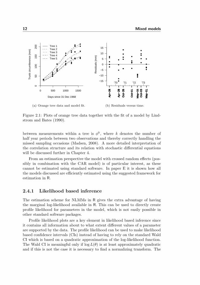
To illustrate the estimation scheme presented in paper E a data set with thegrowth of 5 orange trees is used (Draper and Smith, 1981). The circumferencesof the trees are measured 7 times approximately every half year over a 4 yearperiod. The data has been used previously in the literature by Lindstrom andBates (1990) (see Figure 2.1) and Millar (2004) for illustration of NLMMs. Theformer uses a single random effect for difference in asymptotic circumference andthe latter introduces an additional crossed random effect to handle differencebetween sampling occasions.
In paper E it is shown that the apparently random effect of the samplingoccasion can in fact be explained by a deterministic effect of season and the factthat some half year intervals are missed making the effect look ’random’. It isalso found that residuals within trees are strongly correlated in time which canbe modelled using a continuous auto-regressive (CAR) model given as
cov(εij , εik) = σ2 exp(−φ|tj′ − tj |) (2.13)
where tj is time in days for the jth observations of the ith tree. The resultingmodel is similar to a model proposed for repeated measurements of growth of ratssuggested by Diggle (1988) which includes a random effect for variation betweenrats and serial correlation. Although a continuous AR model is chosen here, asimilar model could be achieved using a discrete AR model where the correlation
12 Mixed models
0 500 1000 1500
050
100
150
200
Days since 31 Dec 1968
Tru
nk c
ircum
fere
nce
(mm
)
Tree 1Tree 2Tree 3Tree 4Tree 5
(a) Orange tree data and model fit.
Res
idua
ls (
mm
)
−15
−10
−5
0
5
10
15
Apr
−28
Apr
−28
Apr
−28
Apr
−28
Apr
−28
Apr
−29
Apr
−29
Apr
−29
Apr
−29
Apr
−29
Oct
−26
Oct
−26
Oct
−26
Oct
−26
Oct
−26
Oct
−01
Oct
−01
Oct
−01
Oct
−01
Oct
−01
May
−15
May
−15
May
−15
May
−15
May
−15
Oct
−03
Oct
−03
Oct
−03
Oct
−03
Oct
−03
May
−01
May
−01
May
−01
May
−01
May
−01
’70 ’71 ’72 ’73
(b) Residuals versus time.
Figure 2.1: Plots of orange tree data together with the fit of a model by Lind-strom and Bates (1990).
between measurements within a tree is φk, where k denotes the number ofhalf year periods between two observations and thereby correctly handling themissed sampling occasions (Madsen, 2008). A more detailed interpretation ofthe correlation structure and its relation with stochastic differential equationswill be discussed further in Chapter 4.
From an estimation perspective the model with crossed random effects (pos-sibly in combination with the CAR model) is of particular interest, as thesecannot be estimated using standard software. In paper E it is shown how allthe models discussed are efficiently estimated using the suggested framework forestimation in R.
2.4.1 Likelihood based inference
The estimation scheme for NLMMs in R gives the extra advantage of havingthe marginal log-likelihood available in R. This can be used to directly createprofile likelihood for parameters in the model, which is not easily possible inother standard software packages.
Profile likelihood plots are a key element in likelihood based inference sinceit contains all information about to what extent different values of a parameterare supported by the data. The profile likelihood can be used to make likelihoodbased confidence intervals (CIs) instead of having to rely on the standard WaldCI which is based on a quadratic approximation of the log-likelihood function.The Wald CI is meaningful only if logL(θ) is at least approximately quadraticand if this is not the case it is necessary to find a normalizing transform. The

2.4 The nonlinear mixed model 13
likelihood confidence interval is superior to the Wald approximation in the sensethat it automatically employs the best possible normalizing transform withoutneeding to know it. The likelihood CI is thus always as good as or betterthan the Wald CI and will thus also better approximate the advertised coverageprobability (Pawitan, 2001).
These well established aspects of likelihood based inference touch upon animportant issue of how to make inference based on collected data in general.This has been the focus of much debate and controversy through out the historyof statistics. It is still a highly relevant research area and thus deserves somediscussion.
Traditionally statistical results have been reported using either Fisher’s p-value for measuring evidence against a null-hypothesis or using the Neyman-Pearson hypothesis testing for choosing between a null and alternative hypoth-esis using a decision rule that controls the long term error rates (Blume andPeipert, 2003). Although the two approaches are fundamentally different in ob-jective they are numerically closely related and this has led to some confusion.If a researcher chooses a significance level α = 0.05 and finds p = 0.0003 afterconducting the study he can with confidence act as if the alternative hypoth-esis is true with assurance given by the long term error rates. However, as aresearcher he might also at the same time argue that the small p-value providesevidence against the null hypothesis in the particular study at hand (as arguedby Fisher). This is wrong however: a single number cannot both be seen from ashort and long run perspective. More detailed arguments for this can be foundin Goodman (1999).
A part from the confusion caused by the mix of the two methods, none ofthem serve typical research purposes well. General research is not a matterof making decisions and also the p-value is easily misleading since it does notreveal any information about the range of effect sizes supported by data. Thishas led to a greater focus on reporting results using confidence intervals, profilelikelihood and other likelihood based methods (Royall, 1997) as these methodsmore adequately convey the statistical evidence available in the data. Theestimation framework presented in paper E supports these ideas by makingfurther analysis of the likelihood function in mixed models directly available.
2.4.2 Computational aspects
The computational complexity of using the mixed modelling framework willalways be somewhat greater than using the first stage model alone or by e.g.estimating a set of common parameters across individuals simply using a pooledlikelihood. By pooled likelihood for data from M individuals y1, ...,yM is meantthe likelihood function L(θ) =
∏Mi=1 L(θ|yi). With estimation in a mixed model
using the Laplace approximation it is for every evaluation of the marginal like-
14 Mixed models
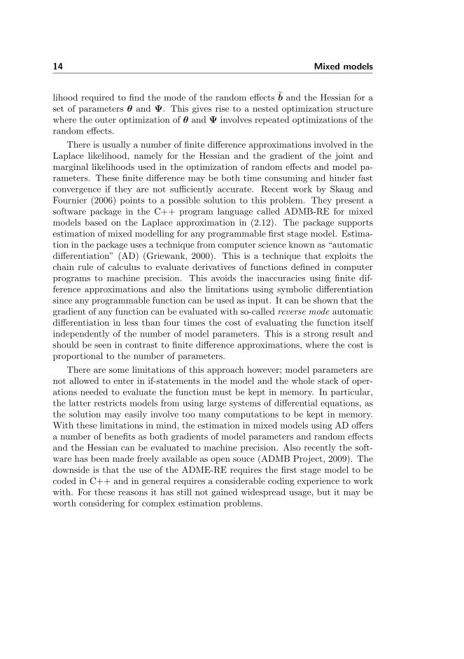
lihood required to find the mode of the random effects b and the Hessian for aset of parameters θ and Ψ. This gives rise to a nested optimization structurewhere the outer optimization of θ and Ψ involves repeated optimizations of therandom effects.
There is usually a number of finite difference approximations involved in theLaplace likelihood, namely for the Hessian and the gradient of the joint andmarginal likelihoods used in the optimization of random effects and model pa-rameters. These finite difference may be both time consuming and hinder fastconvergence if they are not sufficiently accurate. Recent work by Skaug andFournier (2006) points to a possible solution to this problem. They present asoftware package in the C++ program language called ADMB-RE for mixedmodels based on the Laplace approximation in (2.12). The package supportsestimation of mixed modelling for any programmable first stage model. Estima-tion in the package uses a technique from computer science known as “automaticdifferentiation” (AD) (Griewank, 2000). This is a technique that exploits thechain rule of calculus to evaluate derivatives of functions defined in computerprograms to machine precision. This avoids the inaccuracies using finite dif-ference approximations and also the limitations using symbolic differentiationsince any programmable function can be used as input. It can be shown that thegradient of any function can be evaluated with so-called reverse mode automaticdifferentiation in less than four times the cost of evaluating the function itselfindependently of the number of model parameters. This is a strong result andshould be seen in contrast to finite difference approximations, where the cost isproportional to the number of parameters.
There are some limitations of this approach however; model parameters arenot allowed to enter in if-statements in the model and the whole stack of oper-ations needed to evaluate the function must be kept in memory. In particular,the latter restricts models from using large systems of differential equations, asthe solution may easily involve too many computations to be kept in memory.With these limitations in mind, the estimation in mixed models using AD offersa number of benefits as both gradients of model parameters and random effectsand the Hessian can be evaluated to machine precision. Also recently the soft-ware has been made freely available as open souce (ADMB Project, 2009). Thedownside is that the use of the ADME-RE requires the first stage model to becoded in C++ and in general requires a considerable coding experience to workwith. For these reasons it has still not gained widespread usage, but it may beworth considering for complex estimation problems.

Chapter 3
Inhomogeneous Markovprocesses
A Markov process is a stochastic process where all information on the pastrelevant for predicting future states is given by the current state alone. Theprocess is thus independent of how the process arrived at the current state andhow long it has remained there. This property is called the Markov propertyand is named after the Russian mathematician Andrey Markov (1856-1922) whowas the first to study such processes.
For a stochastic process it holds that information about the future state ofthe process is described in probabilistic terms as conditional probabilities. Thestate space for the stochastic process may be either continuous or discrete andthe process may evolve in either continuous or discrete time. Markov processesin continuous time with continuous state space can for a certain class of thesemodels be described using stochastic differential equations and this will be thetopic of Chapter 4. This chapter will focus on Markov processes with a discretestate space and both discrete and continuous time versions will be discussed.When it is necessary to differentiate, the discrete state process in continuoustime is referred to as a Markov jump process and in discrete time simply as aMarkov chain.
Markov processes are divided into two further broad categories; it can beeither time homogeneous or time inhomogeneous. For a homogeneous Markovchain the transition probabilities over a fixed time interval is independent oftime which is not required for an inhomogeneous Markov chain. In this chapter

16 Inhomogeneous Markov processes
it will be shown how an inhomogeneous Markov jump process can be usedas a model for sleep stages and how time changes of parameters defining theinhomogeneous model can be estimated efficiently using a method based on localkernel estimation.
3.1 Sleep EEG
The motivational application for the project is the study of sleep EEG. Anelectroencephalogram (EEG) records electrical activity of the brain’s surfacethrough electrodes placed on designated sites on the scalp. It can be used onboth humans and animals to study the activity of the brain and it can be usedboth for wake and sleeping subjects, but the application here is focused only onthe sleep EEG. The frequency content of a recorded sleep EEG signal usuallyvaries from 1 to 30 Hz and the amplitude of the signal ranges from 20µV to100µV (Forehand, 2003). The frequency and amplitude varies during the nightand based on the frequency range and amplitude of the wave they are denoted asdelta (0.5-4Hz), theta (4-7Hz), alpha (8-13Hz), and beta (13-30Hz) waves withthe highest amplitude for theta waves and the lowest for beta waves. When thebrain is active there is mainly high frequency content, whereas inactivity resultsin a synchronized pattern of low frequency.
Based on the types of waves and other events in the sleep EEG the signal canbe classified into stages relating to ’the state of consciousness’ with is typicallydone for epochs of 10 to 30 seconds. There are two general types of sleep statescalled REM (rapid eye movement) sleep and NREM (Non REM) sleep. Forhumans NREM sleep is further categorized into four sub-states denoted sleepstates I through IV. State I is a transitional state between wake and state II,which is the first true sleep state. States III and IV are the deep sleep stages,often collectively denoted slow wave sleep (SWS) where there is mainly deltaactivity in the signal. REM sleep is distinctively different from NREM sleepas the EEG signal shows high activity resembling wake. The body is relativelyparalyzed during REM sleep with low muscle tone except for the occurrence ofrapid eye movements. REM sleep is found in most mammals and is thoughtto be important for learning and is also the time during which dreams occur(Brodal, 2001). It is sometimes referred to as paradoxical sleep due the seemingcontradictions in its characteristics.
Human sleep cycles through the NREM sleep stages and back to REM sleepabout every 90 minutes whereas rats can go from wake to sleep and back withinminutes. This more fractured sleeping pattern for smaller animals is likely anatural effects of the fact that they need to stay more alert during sleep. Inhumans the sleep structure changes with age and also show individual differences(Brodal, 2001).
The concept of dividing sleep into a number of states for a certain epoch
3.1 Sleep EEG 17
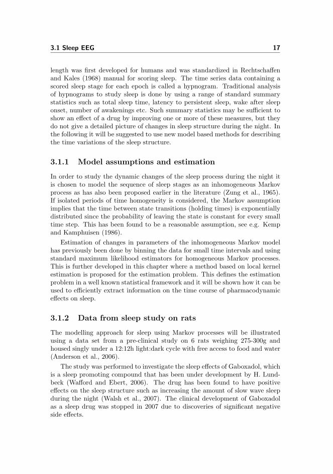
length was first developed for humans and was standardized in Rechtschaffenand Kales (1968) manual for scoring sleep. The time series data containing ascored sleep stage for each epoch is called a hypnogram. Traditional analysisof hypnograms to study sleep is done by using a range of standard summarystatistics such as total sleep time, latency to persistent sleep, wake after sleeponset, number of awakenings etc. Such summary statistics may be sufficient toshow an effect of a drug by improving one or more of these measures, but theydo not give a detailed picture of changes in sleep structure during the night. Inthe following it will be suggested to use new model based methods for describingthe time variations of the sleep structure.
3.1.1 Model assumptions and estimation
In order to study the dynamic changes of the sleep process during the night itis chosen to model the sequence of sleep stages as an inhomogeneous Markovprocess as has also been proposed earlier in the literature (Zung et al., 1965).If isolated periods of time homogeneity is considered, the Markov assumptionimplies that the time between state transitions (holding times) is exponentiallydistributed since the probability of leaving the state is constant for every smalltime step. This has been found to be a reasonable assumption, see e.g. Kempand Kamphuisen (1986).
Estimation of changes in parameters of the inhomogeneous Markov modelhas previously been done by binning the data for small time intervals and usingstandard maximum likelihood estimators for homogeneous Markov processes.This is further developed in this chapter where a method based on local kernelestimation is proposed for the estimation problem. This defines the estimationproblem in a well known statistical framework and it will be shown how it can beused to efficiently extract information on the time course of pharmacodynamiceffects on sleep.
3.1.2 Data from sleep study on rats
The modelling approach for sleep using Markov processes will be illustratedusing a data set from a pre-clinical study on 6 rats weighing 275-300g andhoused singly under a 12:12h light:dark cycle with free access to food and water(Anderson et al., 2006).
The study was performed to investigate the sleep effects of Gaboxadol, whichis a sleep promoting compound that has been under development by H. Lund-beck (Wafford and Ebert, 2006). The drug has been found to have positiveeffects on the sleep structure such as increasing the amount of slow wave sleepduring the night (Walsh et al., 2007). The clinical development of Gaboxadolas a sleep drug was stopped in 2007 due to discoveries of significant negativeside effects.
18 Inhomogeneous Markov processes
The 6 rats are each observed for two 23.5 hour periods. Three of the rats ratsare treated with placebo in the first period and an oral dose (PO) of 20µg/gGaboxadol at the beginning of the second period. The other three rats aretreated in the reverse order and thus all rats are observed for both a placeboand treatment period. During the first 12 hours the light is kept on, and in theremaining time the light is turned off. Rats are most active in the dark, and thestudy design thereby resembles a human taking a sleep drug before bed time.
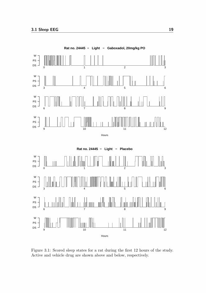
The sleep cycle of the rats is monitored using EEG. The EEG signal is mea-sured with two electrodes implanted in the rat skull and the signal is transmittedusing a telemetry device so that the rats can move freely without any wires at-tached. Based on the EEG three states are classified, namely wake (W), deltasleep (DS) and paradoxical sleep (PS). The DS state corresponds to NREMsleep in humans. These states are determined every 10 seconds giving 8,460equidistantly spaced observations for each rat. An example of data from onerat during the first 12 hours is shown in Figure 3.1 for both active drug andplacebo treatment. This figure corresponds to the hypnogram for the rat andcontains the time series of observed sleep states that will be modelled using aMarkov process.
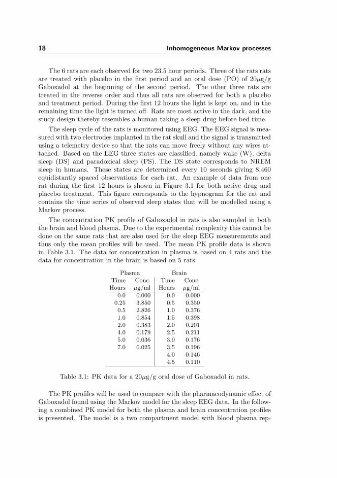
The concentration PK profile of Gaboxadol in rats is also sampled in boththe brain and blood plasma. Due to the experimental complexity this cannot bedone on the same rats that are also used for the sleep EEG measurements andthus only the mean profiles will be used. The mean PK profile data is shownin Table 3.1. The data for concentration in plasma is based on 4 rats and thedata for concentration in the brain is based on 5 rats.
Plasma BrainTime Conc. Time Conc.Hours µg/ml Hours µg/ml
0.0 0.000 0.0 0.0000.25 3.850 0.5 0.3500.5 2.826 1.0 0.3761.0 0.854 1.5 0.3982.0 0.383 2.0 0.2014.0 0.179 2.5 0.2115.0 0.036 3.0 0.1767.0 0.025 3.5 0.196
4.0 0.1464.5 0.110
Table 3.1: PK data for a 20µg/g oral dose of Gaboxadol in rats.
The PK profiles will be used to compare with the pharmacodynamic effect ofGaboxadol found using the Markov model for the sleep EEG data. In the follow-ing a combined PK model for both the plasma and brain concentration profilesis presented. The model is a two compartment model with blood plasma rep-
3.1 Sleep EEG 19
Rat no. 24445 − Light − Gaboxadol, 20mg/kg PO
DS
PS
W
0 1 2 3
DS
PS
W
3 4 5 6
DS
PS
W
6 7 8 9
DS
PS
W
9 10 11 12
Hours
Rat no. 24445 − Light − Placebo
DS
PS
W
0 1 2 3
DS
PS
W
3 4 5 6
DS
PS
W
6 7 8 9
DS
PS
W
9 10 11 12
Hours
Figure 3.1: Scored sleep states for a rat during the first 12 hours of the study.Active and vehicle drug are shown above and below, respectively.

20 Inhomogeneous Markov processes
resented by the central compartment and brain in the peripheral compartment.The orally dosed drug is assumed to be absorbed in the plasma through a firstorder process. The only route of elimination is through the central compart-ment which gives the plasma concentration a double exponential decay profile.The model is illustrated in Figure 3.2 and the corresponding model for the masstransfer of Gaboxadol in the system is given as
dAs/dt = −kaAsdAp/dt = kaAs − (ke + k12)Ap + k21Ab (3.1)dAb/dt = k12Ap − k21Ab.
The unit for the compartments is [A] = µg/g which is understood as amountof drug per gram rat since the dose is weight normalized and the units for therate constants are [k] = min−1.
Stomach
As
ka Plasma
Ap Cp
Brain
Ab Cb
k12
k21
ke
Figure 3.2: PK model for Gaboxadol concentration profiles.
The observations are assumed to be measured with a log-Gaussian distribu-tion around the median response and, that is, the model residuals are additiveGaussian on the log-scale. The number of parameters is limited by assum-ing equal measurement variance for both plasma and brain concentrations (aresidual analysis of the final model fit indicates that this is a reasonable sim-plification). The volume of distribution for the measurement compartments aredenoted Vp and Vb for plasma and brain respectively with a weight normal-ized unit of [V ] = ml/g due to the weight normalized specification of the dose.This gives the observations the correct unit of [C] = µg/ml. The measurementequations are given as
Cp = Ap/Vp exp(εp), (3.2)Cb = Ab/Vb exp(εb).
where [εp εb]T ∼ N(0, σ2I). An additive error model on the original scale for theconcentrations was also tried, but since the range of the concentration values isrelatively large (3.85 to 0.03 µg/ml) this was found to give too large standardizedresiduals for the observations in the top of the range and the log-Gaussian modelwas thus preferred.

3.1 Sleep EEG 21
The model has a total of 7 parameters for the 16 observations excludingthe two zero observations as these cannot be included in the log-Gaussian errormodel. The zero concentration observations at time zero are however implicitlyassumed by the model and it will thus not affect the fit. The model is estimatedby defining the likelihood function in R and maximizing it using R’s built inoptimizer nlminb. The parameter estimates are shown in Table 3.2. The bloodplasma volume Vp is estimated as 6.3% of the body mass and this correspondswell to an approximate value of 7% that is a commonly used reference value(Lee and Blaufox, 1985). The brain volume Vb is estimated to be much largerthan the blood volume and indicates that Gaboxadol is bound in the brain in aform where it is not measured. The smallest rate constant is k21 and the releasefrom the brain is thus the rate limiting step.
The fit of the model is shown in Figure 3.3 and in Figure 3.4 the fit is shownon log-scale. In particular from Figure 3.4 it can be noticed how the doubleexponential decay in the plasma concentration seems to fit well to the observedPK profile. Also, since the release from the brain is the rate limiting step theterminal slopes in both compartments are identical (Gabrielsson and Weiner,2006). This is illustrated in Figure 3.4 where the brain PK curve is inserted asa dotted line together with the plasma PK curve.
ka 2.082 min−1
ke 80.132 min−1
k12 29.292 min−1
k21 0.624 min−1
Vp 0.063 ml/gVb 8.943 ml/gσ 0.255 log µg/ml
Table 3.2: Parameter estimates for Gaboxadol PK model.
0 2 4 6 8
0
5
10
15
20
Hours
Sto
mac
h (µ
gg)
0 2 4 6 8
0
1
2
3
4
5
6
Hours
Pla
sma
(µg
ml)
0 2 4 6 8
0.0
0.1
0.2
0.3
0.4
0.5
Hours
Bra
in (µ
gm
l)
Figure 3.3: PK model for Gaboxadol.

22 Inhomogeneous Markov processes
0 2 4 6 8
0.010.02
0.050.100.20
0.501.002.00
5.00
Hours
Pla
sma
(µg
ml)
0 2 4 6 8
0.05
0.10
0.20
0.50
Hours
Bra
in (µ
gm
l)Figure 3.4: PK model for Gaboxadol shown on log-scale. The brain PK curve(right) is inserted as a dotted line together with the plasma PK curve (left).
3.1.3 Discrete versus continuous time
As discussed at the beginning of this chapter the Markov process assumed togenerate the observed hypnograms can be modelled in either discrete or con-tinuous time. In this thesis it is chosen to mainly work with the continuousrepresentation for reasons which is argued as follows:
It is not realistic to think that the real sleep process is separated into epochsof an arbitrary length of either e.g. ten or thirty seconds. Sleep is a continuousprocess and should thus also be modelled as such (Kemp and Kamphuisen,1986). Of course the scoring of sleep into a number of states is in itself anabstraction and interpretation of the data, but it is appealing to think of thesleep states as a process describing the state of consciousness of the body whichmay change at any time point and which it is simply chosen to sample at discretetime points.
Moreover, the continuous representation makes the parameterization inde-pendent of the sampling period which is not the case for a discrete time rep-resentation. This is because the continuous process is parameterized by raterelated parameters related to the expected time until next state change whereasthe discrete process is defined in terms of probabilities directly related to thesampling interval. For this reason the continuous time parameters may also beeasier to relate to without an in-depth understanding of Markov processes.
Finally if the actual process is evolving in continuous time and have con-straints on the possible jumps so that not all jumps between all states areallowed this can be directly included in the continuous time model representa-tion. If the model is described in discrete time this may not be the case, sincethe process may change to any state in a series of jumps and thus such physicalrestrictions are more difficult or impossible to make use of in a discrete modelof the process.
3.2 Model definition 23
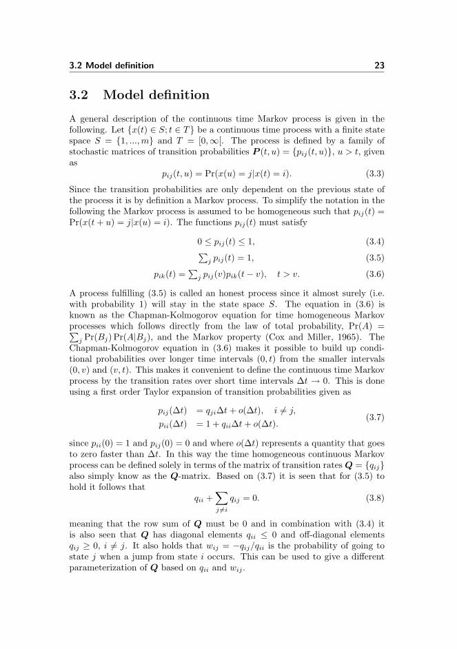
3.2 Model definition
A general description of the continuous time Markov process is given in thefollowing. Let x(t) ∈ S; t ∈ T be a continuous time process with a finite statespace S = 1, ...,m and T = [0,∞[. The process is defined by a family ofstochastic matrices of transition probabilities P (t, u) = pij(t, u), u > t, givenas
pij(t, u) = Pr(x(u) = j|x(t) = i). (3.3)
Since the transition probabilities are only dependent on the previous state ofthe process it is by definition a Markov process. To simplify the notation in thefollowing the Markov process is assumed to be homogeneous such that pij(t) =Pr(x(t+ u) = j|x(u) = i). The functions pij(t) must satisfy
0 ≤ pij(t) ≤ 1, (3.4)∑j pij(t) = 1, (3.5)
pik(t) =∑j pij(v)pik(t− v), t > v. (3.6)
A process fulfilling (3.5) is called an honest process since it almost surely (i.e.with probability 1) will stay in the state space S. The equation in (3.6) isknown as the Chapman-Kolmogorov equation for time homogeneous Markovprocesses which follows directly from the law of total probability, Pr(A) =∑j Pr(Bj) Pr(A|Bj), and the Markov property (Cox and Miller, 1965). The
Chapman-Kolmogorov equation in (3.6) makes it possible to build up condi-tional probabilities over longer time intervals (0, t) from the smaller intervals(0, v) and (v, t). This makes it convenient to define the continuous time Markovprocess by the transition rates over short time intervals ∆t → 0. This is doneusing a first order Taylor expansion of transition probabilities given as
pij(∆t) = qji∆t+ o(∆t), i 6= j,
pii(∆t) = 1 + qii∆t+ o(∆t).(3.7)
since pii(0) = 1 and pij(0) = 0 and where o(∆t) represents a quantity that goesto zero faster than ∆t. In this way the time homogeneous continuous Markovprocess can be defined solely in terms of the matrix of transition rates Q = qijalso simply know as the Q-matrix. Based on (3.7) it is seen that for (3.5) tohold it follows that
qii +∑j 6=i
qij = 0. (3.8)
meaning that the row sum of Q must be 0 and in combination with (3.4) itis also seen that Q has diagonal elements qii ≤ 0 and off-diagonal elementsqij ≥ 0, i 6= j. It also holds that wij = −qij/qii is the probability of going tostate j when a jump from state i occurs. This can be used to give a differentparameterization of Q based on qii and wij .

24 Inhomogeneous Markov processes
Using (3.7) it is possible to find transition probabilities for very small timesteps ∆t. To extend this to arbitrary time steps it is necessary to define theforward equations. Suppose that the process starts at state i, x(0) = i, and thatpij(t) = Pr(x(t) = j|x(0) = i). Using (3.6) for ∆t > 0 this gives
pik(t+ ∆t) = pik(t)(1 + qkk∆t) +∑j 6=k
pik(t)qjk∆t+ o(∆t), (3.9)
where the first term is the probability of going directly from i to k and stayingthere and the last term is the probability of going from i to j and then to k.Letting ∆t→ 0 in (3.9) results in p′ik(t) =
∑j pij(t)qjk and in matrix notation
this is written asP ′(t) = P (t)Q (3.10)
with initial condition P (0) = I. If a time inhomogeneous Markov process isconsidered the equation generalizes to
∂
∂uP (t, u) = P (t, u)Q(u), (3.11)
which is known as the Kolmogorov forward differential equation. For a givenQ(t) the conditional probabilities governing the process is thus completely de-scribed using (3.11). It can be shown that if Q(t) is time invariant then timebetween jumps (holding times) are exponentially distributed and that the diag-onal elements qii(t) of Q(t) contains the negative rate for leaving a state. Thisfollows from (3.7) since the probability of staying in the same state in any in-terval ∆t is 1 + qii∆t which gives a geometric distribution of holding times for∆t > 0 and an exponential distribution for ∆t→ 0.
3.2.1 Likelihood estimation
The process x(t) is observed at N discrete time points that are chosen indepen-dent of the observed process. The model dynamics are assumed to be slowlyvarying relative to the time between observations. The observation sequence isdenoted xk and contains the state at time tk where k = 1, ..., N .
The likelihood function is formed as a product of conditional densities thatcan be found using (3.11) and is given as
L(Q(t)) =∏N−1k=1 Lk(Q(t)) (3.12)
=∏N−1k=1 p(xk+1|xk) (3.13)
This likelihood function is called a conditional likelihood function since it isdefined conditional on the first observation.
As noted above, the model dynamics are assumed to be slowly varying rel-ative to the time between observations. This has the implication that Q(t)

3.2 Model definition 25
for tk ≤ t ≤ tk+1 can be assumed constant between two observations so thatQk = Q(tk). With this approximation the transition probabilities in (3.13) canbe found using the forward equations in (3.10) as
P (tk, tk+1) = exp(∆tkQk) (3.14)
where ∆tk = tk+1− tk and exp(·) denotes the matrix exponential. The approxi-mation avoids solving the partial differential equations in (3.11). If ∆tk is largerrelative to the time variations of Q(t) one can also choose to use a first or higherorder expansion of Q(t) which also has an explicit solution for the transitionprobabilities.
3.2.2 The imbedding problem for Markov chains
For estimation problems where it is assumed that the Markov process evolves incontinuous time it could seem tempting to estimate the transition probabilitiesdirectly instead of estimating parameters in the continuous time representationwhere the matrix exponential is involved. However, this leads to problems sincethe matrix exponential is not a one-to-one transformation and this is related tothe imbedding problem for Markov chains.
The imbedding problem for Markov chains is the question about whether agiven discrete time Markov chain can be obtained by discrete time sampling ofa continuous time Markov jump process. The imbedding problem has receivedmuch attention within theoretical analysis of Markov processes going back toElfving (1937) and later e.g. Kingman (1962) and the problem is also relevantin the present context of estimating parameters using maximum likelihood.
To clarify the problem it is illustrated for a time homogeneous process whichis observed with a constant sampling interval ∆t (Bladt and Sørensen, 2005). Ifit is assumed that the observations come from a Markov process in continuoustime the parameters Q are estimated using the likelihood function in (3.13).The transition probabilities are constant due to a constant Q and ∆t and areestimated as exp(∆tQ) where Q is the MLE of Q. If it is instead assumedthat the observed sequence of states comes from a Markov process in discretetime, the parameters to be estimated are directly the transition probabilitiesP d, which define a discrete time Markov process. It can be shown that themaximum likelihood estimate is given as P d = nij/ni. where nij denotes thenumber of jumps from i to j and ni. the total number of jumps from i.
If there exist a Q fulfilling the criteria for an intensity matrix and suchthat P d = exp(∆tQ) then this Q is the MLE Q. However, the equation willnot always have a solution, in which case the estimated P d does not representtransition probabilities that can be obtained from a continuous time Markovchain. Exactly defining the set matrices P d where the equation can be solvedgiven the constraints on Q is a difficult problem, but a simple and sufficient

26 Inhomogeneous Markov processes
criterion is that all diagonal elements of P d are ≥ 1/2 (Cuthbert, 1973). Thisindicates that the problem is related to the sampling frequency, since a fastersampling will result in higher diagonal probabilities.
This discussion emphasizes the necessity of estimating parameters in thecontinuous time representation if this is the model that should be used forinference and in particular if the actual process is known to evolve in continuoustime. The continuous time representation involves the extra complexity of usingthe matrix exponential to evaluate the likelihood function but insures that theestimated parameters will in fact represent a continuous time Markov process.
3.3 Non-parametric estimation
Until now estimation of the time varying Q(t) matrix has been referred to with-out a specific parameterization in mind. The problem of finding a suitableparameterization is in some sense comparable to the problem of finding a suit-able regression function in non-linear least squares regression based on a set ofobservations. The problem here is that it is not possible to get a visual impres-sion of the time variations of Q(t) by plotting the observed data (see e.g. Figure3.1) since the rate related parameters of Q(t) cannot be directly related to theindividual observations.
To overcome this problem the data can be separated in small time segmentswhere the parameters of the intensity matrix can be estimated by assuming alocally time homogeneous process. This approach is used in Kemp and Kam-phuisen (1986) for clinical hypnogram data and in Madsen et al. (1985) forobservations of cloud cover and results in rough estimates of the time varia-tions.
In paper D an improved method for estimation of the time variations of Q(t)is presented. The method is based on a locally weighted likelihood function to-gether with a polynomial approximation of the parameters defining Q(t). Themethod is generally applicable for local estimation in continuous time Markovprocesses and has a number of advantages in comparison to more simple ap-proaches as the one described above. It is possible to use any choice of kernelfor weighing the data and the use of higher order polynomials makes the methodmore capable of capturing rapid changes in the Q(t) matrix. A typical problemwhen doing local estimation using e.g. a zero or first order polynomial is thatestimates of peaks will be negatively biased since this shape is not well approx-imated by these lower order polynomials. To avoid this problem it is necessaryto use a relatively smaller bandwidth which on the other hand results in a largervariation in the estimates. A second order polynomial is naturally a much bet-ter approximation around peaks also for larger bandwidths, which gives morerobust estimates since it is possible to use a larger bandwidth without increasingthe bias in same way as for the low order polynomial approximations. In paper

3.3 Non-parametric estimation 27
D there is a comparison of the results of estimation using 0th, 1st, and 2ndorder polynomials where it is seen how the 2nd order approximation is muchmore sensitive to peaks in the parameters.
The method for local estimation method in paper D uses a set of parametersβ which defines the local polynomials used to describe the time variations Q(t)around a time point of interest tc. As in ordinary local estimation methods theidea is to find a local estimate of Q(tc) by estimating the parameters β usinglocally weighted data. To get a complete picture of the time variations in Q(t)the method is repeated for a series of suitably close values of tc ∈ T .
The local estimation method for inhomogeneous Markov processes will beoutlined in the following in order to provide the basis for discussing extensionsof the methods for choosing bandwidth presented in paper D.
3.3.1 Choice of bandwidth
The likelihood function for the local estimation method at a given time pointof interest tc is defined as
logL(β, tc) =N−1∑k=1
w(xk, tc) logLk(β) (3.15)
where Lk is the likelihood of a single observed transition defined in (3.13). Theweights for the observed transitions are w(xk, tc) and are found as
w(xk, tc) = Kh(xk)(tk − tc). (3.16)
The kernel function K is a symmetric probability function and h(xk) is a statedependent bandwidth. The bandwidth defines the size of the local neighborhoodby scaling the kernel function as Kh(t) = K(t/h)/h (Fan and Gijbels, 1996).
The definition of the weights in (3.16) as state dependent is an extensionto the definition in paper D, where the weights are simply defined as wk(tc) =Kh(tk − tc) independently of the observed state.
The reason for introducing the state dependent bandwidth is that informa-tion about the ith row in Q(t) is mainly contained in the observed transitionsfrom state i. If there are no observations of transitions from state i it is notpossible to estimate any parameters for state i related to holding times or prob-abilities of jumping to other states. Conversely, if many observations of tran-sitions from state i are available in the data the ith row in Q(t) will be welldefined. By using a state dependent bandwidth it is possible to define localbandwidths that include a more even amount of information about the individ-ual states and thereby making the method more equally local for all parametersto be estimated.
Two methods for state dependent bandwidth are considered. The bandwidthfor a state i can be chosen such that the interval tc ± h(i) contains either

28 Inhomogeneous Markov processes
1. a total of M observations of state i, or,
2. a fixed proportion α of the observations of state i (denoted nearest neigh-bor (NN) bandwidth).
With Method 1 it may happen that M is larger than the observed number ofjumps from a state, that is M > ni. for some i ∈ S. To handle this smoothlythe bandwidth is increased for these states by a factor M/ni. of the bandwidthcovering all observations. In this way the kernel weights given in (3.16) will evenout and approach a constant within the observation window for h → ∞. Theapproximation of parameters with only very limited information will thus tendtoward a global polynomial representation.
Methods 1 and 2 differ in that the first method aims at using an equalamount of information to estimate parameters for each state, whereas the secondmethod will use a fixed proportion of the information available for each state.The preferred method will depend on the application at hand.
In paper D an example of a non-parametric estimation of the Q matrix forthe EEG hypnogram data from the study of Gaboxadol in rats is illustrated. Theestimation is performed by pooling all data from the six rats to give estimatesof the mean effects in the data. Only the treatment data is used giving a totalof 8, 460×6 = 50, 760 observations. The parameterization of Q is given in termsof q1(t) for the rate for leaving state i and wi for the probability of jumpingto i − 1 when a transition occurs. The parameter w1 = 0 since physiologicallyjumps from W to PS should not occur and this can be implemented directly inthe continuous time representation. The model is thus defined as
f : θ(t) → Q(t) :
Q(t) =
−q1(t) q1(t) 0w2(t)q2(t) −q2(t) (1− w2(t))q2(t)
(1− w3(t))q3(t) w3(t)q3(t) −q3(t)
qi(t) = exp[θi(t)], i = 1, 2, 3
wi(t) = logit−1[θi+2(t)], i = 2, 3 ,
(3.17)
where the parameters θ(t) = [θ1(t), ..., θ5(t)] are estimated locally using 2ndorder polynomials defined by the parameters in β. With 5 parameters in themodel and using 2nd order polynomials this gives a total of 15 parameters in βthat is estimated for every time point tc. When defining the parameterization ofthe model it is necessary to make the model unbounded in the θ(t) parameterswhich is done here using the exponential and logit transform for the rate andprobability parameters respectively. If the model is not unbounded in θ(t)the polynomial representation of these parameters may easily give values ofthe parameters where the model cannot be evaluated to find the transitionprobabilities.

3.3 Non-parametric estimation 29
In paper D the parameters [θ1(t), ..., θ5(t)] are estimated locally using 2ndorder polynomials and a state independent NN bandwidth of α = 0.40 of thetotal number of observations. The result is seen in Figure 3.5. For comparison,the result of estimation using the state dependent bandwidth in Method 1 withM = 6000 and using 2nd order polynomials is shown in Figure 3.6 with thebandwidth for the individual states shown in the last row. For both figures atricube kernel function has been used. For the NN method using α = 0.40the bandwidth is constantly 0.40× 23.5 h. = 9.4 hours since the sampling timesare equidistant For the state dependent bandwidth the bandwidth varies sincethe frequency of visits to the three states differ throughout the time period. Inparticular it is seen that the bandwidth is as low as 3-4 hours for the DS stateduring the initial 12 hours and using the 2nd order polynomial this gives a muchmore apparent effect peak in expected time in the DS state with a maximum ofmore than 12 minutes compared to 6 minutes for NN method.
For the PS state there is only a total of 1343 observations ( M) giving aconstant bandwidth of 23.5 h × 6000/1343 = 105 hours. This results in tricubeweights between 1 and 0.9955 for a 24 hour range which again results in almostglobal polynomial approximations for the two parameters related to the PSstate. The global estimates for the two parameters q3 and w3 for the PS stateare thus similar to 2nd order polynomials that has been either log or inverse-logit transformed but deviations are still seen since the estimates are correlatedwith the other more locally estimated parameters.
3.3.1.1 Relation of effect to the PK-profile
To compare the effect of Gaboxadol on the non-parametric estimates of the sleepparameters the analysis has been carried out on both placebo and treatmentdata. The results are shown in Figure 3.7 using M = 6000, the same as used forFigure 3.6. It is seen that the most apparent effect of Gaboxadol is found in theestimates of the expected time in the DS state. The significant peak between 0and 6 hours is only found in the treatment data, whereas the placebo data seemsto be rather constant during this period. The effect on the expected time inthe DS state can thus be attributed to Gaboxadol, and it is thereforeinterestingto see how the estimated effect relates to the mean PK concentration profile ofGaboxadol in the brain which is modelled in Section 3.1.2.
In Figure 3.8 the expected time in the sleep state DS is compared with thePK profile of Gaboxadol in the brain. The figure indicates that there is a directrelation between the PK profile and the expected time in the DS state with adelay of approximately one hour. The indication of this relation directly benefitsfrom the high temporal resolution and sensitivity of the estimate of the expectedtime in DS found using the non-parametric local estimation method.
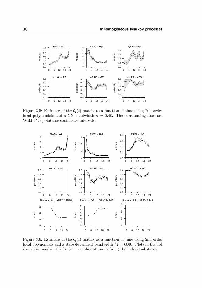
30 Inhomogeneous Markov processes
Min
utes
0.00.51.01.52.02.53.03.5
0 6 12 18 24
E(W) = 1/q1
Min
utes
01234567
0 6 12 18 24
E(DS) = 1/q2
Min
utes
0.0
0.1
0.2
0.3
0.4
0 6 12 18 24
E(PS) = 1/q3
prob
abili
ty
0.0
0.2
0.4
0.6
0.8
1.0
0 6 12 18 24
w1: W −> PSpr
obab
ility
0.0
0.2
0.4
0.6
0.8
1.0
0 6 12 18 24
w2: DS −> W
prob
abili
ty
0.0
0.2
0.4
0.6
0.8
1.0
0 6 12 18 24
w3: PS −> DS
Figure 3.5: Estimate of the Q(t) matrix as a function of time using 2nd orderlocal polynomials and a NN bandwidth α = 0.40. The surrounding lines areWald 95% pointwise confidence intervals.
Min
utes
0
1
2
3
4
0 6 12 18 24
E(W) = 1/q1
Min
utes
0
5
10
15
0 6 12 18 24
E(DS) = 1/q2
Min
utes
0.0
0.1
0.2
0.3
0.4
0 6 12 18 24
E(PS) = 1/q3
prob
abili
ty
0.0
0.2
0.4
0.6
0.8
1.0
0 6 12 18 24
w1: W −> PS
prob
abili
ty
0.0
0.2
0.4
0.6
0.8
1.0
0 6 12 18 24
w2: DS −> W
prob
abili
ty
0.0
0.2
0.4
0.6
0.8
1.0
0 6 12 18 24
w3: PS −> DS
Hou
rs
0 6 12 18 24
05
1015
Kernel spanNo. obs W : GBX 14570
Hou
rs
0 6 12 18 24
01
23
45
6
Kernel spanNo. obs DS : GBX 34846
Hou
rs
0 6 12 18 24
040
8012
0
Kernel spanNo. obs PS : GBX 1343
Figure 3.6: Estimate of the Q(t) matrix as a function of time using 2nd orderlocal polynomials and a state dependent bandwidth M = 6000. Plots in the 3rdrow show bandwidths for (and number of jumps from) the individual states.
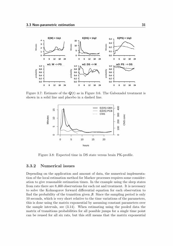
3.3 Non-parametric estimation 31
Min
utes
0
1
2
3
4
0 6 12 18 24
0
1
2
3
4
0 6 12 18 24
E(W) = 1/q1
Min
utes
0
5
10
15
0 6 12 18 24
0
5
10
15
0 6 12 18 24
E(DS) = 1/q2
Min
utes
0.0
0.1
0.2
0.3
0.4
0 6 12 18 24
0.0
0.1
0.2
0.3
0.4
0 6 12 18 24
E(PS) = 1/q3pr
obab
ility
0.0
0.2
0.4
0.6
0.8
1.0
0 6 12 18 24
0.0
0.2
0.4
0.6
0.8
1.0
0 6 12 18 24
w1: W −> PS
prob
abili
ty
0.0
0.2
0.4
0.6
0.8
1.0
0 6 12 18 24
0.0
0.2
0.4
0.6
0.8
1.0
0 6 12 18 24
w2: DS −> W
prob
abili
ty
0.0
0.2
0.4
0.6
0.8
1.0
0 6 12 18 24
0.0
0.2
0.4
0.6
0.8
1.0
0 6 12 18 24
w3: PS −> DS
Figure 3.7: Estimate of the Q(t) as in Figure 3.6. The Gaboxadol treatment isshown in a solid line and placebo in a dashed line.
0 5 10 15 20
05
1015
hours
Min
utes
010
020
030
040
0
CN
S c
onc
E(DS) GBXE(DS) PCBCNS
Figure 3.8: Expected time in DS state versus brain PK-profile.
3.3.2 Numerical issues
Depending on the application and amount of data, the numerical implementa-tion of the local estimation method for Markov processes requires some consider-ation to give reasonable estimation times. In the example using the sleep statesfrom rats there are 8,460 observations for each rat and treatment. It is necessaryto solve the Kolmogorov forward differential equation for each observation tofind the probability of the transition given β. Since the sampling period is only10 seconds, which is very short relative to the time variations of the parameters,this is done using the matrix exponential by assuming constant parameters overthe sample intervals, see (3.14). When estimating using the pooled data thematrix of transitions probabilities for all possible jumps for a single time pointcan be reused for all six rats, but this still means that the matrix exponential
32 Inhomogeneous Markov processes
is evaluated 8,460 times for each evaluation of the likelihood function.The implementation of the local estimation method has been done mainly
in R. The default R installation does not have a matrix exponential function sothe initial work was done using the Matrix package that uses a method by Ward(1977) based on a Pade’ approximation with three preconditioning steps whichhas originally been implemented for Octave (Eaton, 2002).
A small side result from this initial work with the Matrix package was thediscovery of an error in the code which resulted in erroneous evaluations of thematrix exponential that was evident for certain matrices. This was pointed outto Martin Maechler, a member of the R Development Core Team, who was ableto locate the bug which turned out to come from the original Octave code.
The final implementation of the estimation method is partly based on R withthe evaluation of the likelihood function (3.15) including the matrix exponentialbeing done in Fortran. The matrix exponential is evaluated using DGPADM fromExpokit (Sidje, 1998) which uses a Pade approximation to the exponentialfunction combined with scaling-and-squaring (Moler and Van Loan, 1978). Bykeeping the likelihood function solely in Fortran gives a significant speedup.The optimization of the parameters in the likelihood function is done by callinggeneral optimizers from R. This was found as a good compromise between codingcomplexity and flexibility.
The optimization problem is in itself relatively complex. As mentioned thereare a total of 15 parameters in β in the model for the rat EEG data that isestimated for every time point tc and these parameters are all dependent on eachother. The optimization problem at each tc benefit from the fact that they areserially related such that the final estimate of β at tc is a good initial value at thenext tc + ∆t. The estimation of β has been done with a standard quasi-Newtonmethod with BFGS updating of the Hessian for finding the search direction andusing soft line search for finding the next iterate (Nocedal and Wright, 2006).This method generally performs well for optimization of likelihood functions andis available in optim in the stats package in R. The method initializes the Hessianas the identity matrix which is also most commonly done. However, this can beimproved in the serial optimization structure by using the final Hessian estimatefrom the previous tc as the initial estimate in the next optimization. This featureis available for the ucminf method (Nielsen, 2000) and was implemented in Rfor this purpose (Nielsen and Mortensen, 2008). The method works well but itis not found that the improved initial estimate of the Hessian gives a notablereduction in estimation times. The ucminf method were afterwards also usedfor the estimation problems with mixed models in paper E and here it is in factable to outperform optim and nlminb both from the stats package in R.

3.4 Parametric estimation 33
3.4 Parametric estimation
The non-parametric estimates of the time variations of the Markov process canbe used to identify a possibly more simple parametric description of these timevariations. This can be used for modelling the main structures in the parametersby testing for model reduction using a standard likelihood ratio test (Madsen,2008). Also in a parametric model individual variations can be described using amixed model with random effects and the drug effect can be included as functionof the PK concentration profile, which gives the possibility of statistically testingdifferent relations with PK profile for the parameters in the Markov process.
It is noted that the mixed modelling approach modifies the Markov assump-tion to be conditional on the random effects. When the random effects areintegrated out, the process is nolonger of the Markov type. One can see thisas a more flexible class of processes, which can still be interpreded in a Markovframework.
Karlsson et al. (2000) use the parametric approach to describe the sleepstructure in a study of 21 patients that are treated with both placebo andthe sleep drug Temazepam. The modelling is not done in continuous time butinstead in discrete time where each transition probability is modelled separately.This means that for modelling jumps e.g. from state 1 to 2 all data with jumpsfrom state 1 is extracted and it is noted if a jump to state 2 occurs or not.The data for a particular transition from i to j is thus binary yk ∈ 0, 1,k = 1, ..., ni., and the modelling of each transition probability as a function oftime is similar to a logistic regression problem. The main focus of the modellingis to incorporate the drug effect in the model and also to include the individualvariation using Gaussianly distributed random effects. Both the drug effectand random effects are included additively on the logit scale of the transitionprobability which ensures that probabilities are always in the interval [0; 1]. Themodel is fitted using NONMEM to handle the estimation of the mixed model.NONMEM has the possibility of directly specifying the log-likelihood for the firststage model which is given as logL1(b,θ) = ykp
∗ij(b,θ, t)+(1−yk)(1−p∗ij(b,θ, t))
where p∗ij(b,θ, t) denotes the transition probability as a function of the randomeffects b and parameters θ in the model. The model is fitted using the ’Laplace’option in NONMEM which uses the likelihood in (2.12).
The approach in Karlsson et al. (2000) has also been applied to the rat EEGdata to investigate the individual difference between the rats. The transitionfrom DS to W is considered and rough estimates of the individual transitionprobabilities are shown in Figure 3.9. The estimates are found by counting thenumber of transitions from DS to W in two hour intervals and dividing by thenumber of observations of DS in this interval.
The transition probability is modelled with a simple model with two levels
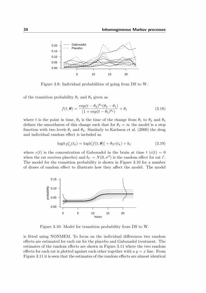
34 Inhomogeneous Markov processes
5 10 15 20
0.00
0.05
0.10
0.15
0.20 GaboxadolPlacebo
Figure 3.9: Individual probabilities of going from DS to W.
of the transition probability θ1 and θ2 given as
f(t,θ) =exp(t− θ3)θ4(θ2 − θ1)
(1 + exp(t− θ3)θ4)+ θ1 (3.18)
where t is the point in time, θ3 is the time of the change from θ1 to θ2 and θ4
defines the smoothness of this change such that for θ4 =∞ the model is a stepfunction with two levels θ1 and θ2. Similarly to Karlsson et al. (2000) the drugand individual random effect is included as
logit p∗ij(tk) = logit[f(t,θ)] + θ5c(tk) + bi′ (3.19)
where c(t) is the concentration of Gaboxadol in the brain at time t (c(t) = 0when the rat receives placebo) and bi′ ∼ N(0, σ2) is the random effect for rat i′.The model for the transition probability is shown in Figure 3.10 for a numberof draws of random effect to illustrate how they affect the model. The model
0 5 10 15 20
0.00
0.05
0.10
0.15
prob
abili
ty
hours
Figure 3.10: Model for transition probability from DS to W.
is fitted using NONMEM. To focus on the individual differences two randomeffects are estimated for each rat for the placebo and Gaboxadol treatment. Theestimates of the random effects are shown in Figure 3.11 where the two randomeffects for each rat is plotted against each other together with a y = x line. FromFigure 3.11 it is seen that the estimates of the random effects are almost identical
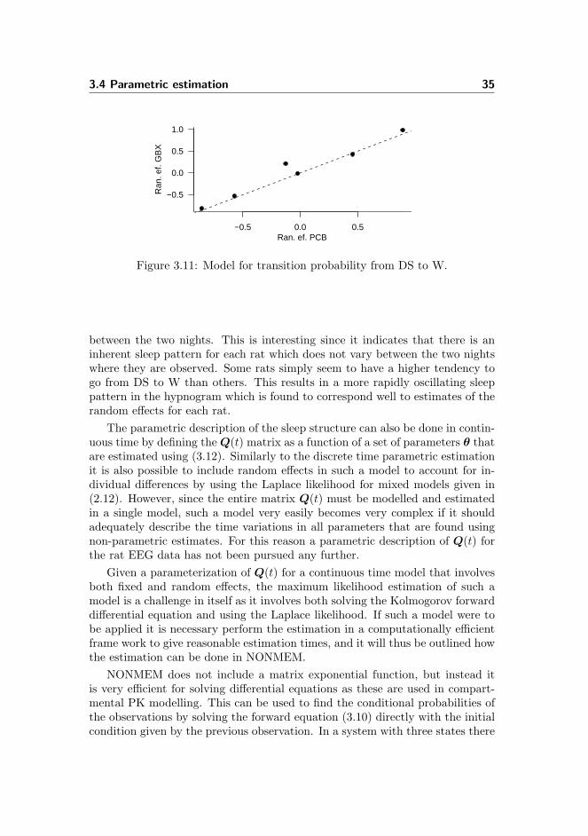
3.4 Parametric estimation 35
−0.5 0.0 0.5
−0.5
0.0
0.5
1.0
Ran
. ef.
GB
X
Ran. ef. PCB
Figure 3.11: Model for transition probability from DS to W.
between the two nights. This is interesting since it indicates that there is aninherent sleep pattern for each rat which does not vary between the two nightswhere they are observed. Some rats simply seem to have a higher tendency togo from DS to W than others. This results in a more rapidly oscillating sleeppattern in the hypnogram which is found to correspond well to estimates of therandom effects for each rat.
The parametric description of the sleep structure can also be done in contin-uous time by defining the Q(t) matrix as a function of a set of parameters θ thatare estimated using (3.12). Similarly to the discrete time parametric estimationit is also possible to include random effects in such a model to account for in-dividual differences by using the Laplace likelihood for mixed models given in(2.12). However, since the entire matrix Q(t) must be modelled and estimatedin a single model, such a model very easily becomes very complex if it shouldadequately describe the time variations in all parameters that are found usingnon-parametric estimates. For this reason a parametric description of Q(t) forthe rat EEG data has not been pursued any further.
Given a parameterization of Q(t) for a continuous time model that involvesboth fixed and random effects, the maximum likelihood estimation of such amodel is a challenge in itself as it involves both solving the Kolmogorov forwarddifferential equation and using the Laplace likelihood. If such a model were tobe applied it is necessary perform the estimation in a computationally efficientframe work to give reasonable estimation times, and it will thus be outlined howthe estimation can be done in NONMEM.
NONMEM does not include a matrix exponential function, but instead itis very efficient for solving differential equations as these are used in compart-mental PK modelling. This can be used to find the conditional probabilities ofthe observations by solving the forward equation (3.10) directly with the initialcondition given by the previous observation. In a system with three states there
36 Inhomogeneous Markov processes
are three differential equations to solve for pi = [pi1 pi2 pi3] given as
d
dtpi = pi
q1 q12 q13
q21 q2 q23
q31 q32 q3
(3.20)
but since the conditional probabilities must sum to 1, it is only necessary to solvetwo of the differential equations to find the probabilities pi1 and pi2. Dependingon the previously observed state the initial condition for [pi1 pi2] will be either[1 0], [0 1] or [0 0] for state 1, 2, and 3, respectively. The forward differentialequations for pi1 and pi2 becomes
d
dt
[pi1pi2
]=[q1 − q31 q21 − q31
q12 − q32 q2 − q32
] [pi1pi2
]+[q31
q32
](3.21)
and they can be derived in a similar way for a system of any size. This systemcan be solved in NONMEM by considering pi1 and pi2 as two pseudo compart-ments which are reset before each observation to [0 0] using a reset event in thedata file and possibly updated to [1 0] or [0 1] with an additional dose eventif the previous observation is either 1 or 2, respectively. When the differentialequations are solved for each observation to give the conditional probabilitiesof the observation, the first stage likelihood can be formed in NONMEM inthe same way as it is done for the discrete time Markov models as discussedpreviously. This approach has been implemented in NONMEM and was foundto estimate the parameters in the Q(t) matrix correctly by testing using simpleparametric models. The estimation method in NONMEM opens up for exper-imentation with the parametric approach for continuous Markov processes incombination with mixed effects modelling, but as mentioned previously this hasnot been pursued further here.
3.5 Discussion
Although local estimation of parameters in an inhomogeneous Markov processis a promising way of extracting information about the sleep process, it shouldstill be kept in mind that any results and interpretations are limited by themodel used for scoring sleep stages.
For human sleep staging the guidelines by Rechtschaffen and Kales has beenstrongly debated over the past many years (Himanen and Hasan, 2000). Theguidelines were developed for healthy adults with undisturbed sleep and thescoring may thus be ambiguous for patients with sleep disturbances. The guide-line in general leaves some room for interpretation and this results in inter-rateragreements around 90% when raters are compared. This observation suggestsusing a hidden Markov model by assuming that stages are observed with mea-surement error.

3.5 Discussion 37
Such a model of observing states with ’noise’ (misclassification) is equivalentto the model with SDEs observed with measurement error as presented in Chap-ter 4. The process defined by SDEs is also Markov but evolves in a continuousspace where as the sleep process only evolves in a small discrete set of sleepstages.
A number of replacements to the Rechtschaffen and Kales guidelines has beensuggested such as Himanen et al. (1999) and Grube et al. (2002). However, noneof these have gained wide spread usage and the original guidelines are thus stillused as the gold standard. The most likely reason for this is that although newmethods may deal with some of the shortcomings in the original guidelines itis still necessary to use them to be able to compare with past results in sleepstudies. For this reason it is very relevant to consider improved analysis of theoriginal sleep stages by using new methods such as the non-parametric approachpresented here. This will help increase the understanding of the underlying sleepprocess while still being kept in a framework that can be related to other resultsin the area.

38 Inhomogeneous Markov processes

Chapter 4
Stochastic differentialequations
Stochastic differential equations (SDEs) represent an extensively studied math-ematical theory that has found a wide range of practical applications. SDEsprovide the tool for building dynamical models based on differential equationswhere it is possible to include some amount of randomness or noise into themodel. A very simple example of such a model is an exponential populationgrowth model where the growth rate is only approximately known and thusloosely given by r(t)+”noise”. The model for the population growth can there-fore be written as da(t)/dt = (r(t) + ”noise”)a(t).
To explain this in popular terms, consider a constant growth rate model,say with a growth of 3%/year. An ordinary differential equation model willconvert this to an exponential formula for the population. If, for some reason,the growth is higher in one year the model implies a reduced growth growth thefollowing year so the population returns to the originally projected curve. AnSDE model will instead accept the higher growth rate in that year and use theactual population as the base for future growth, applying and expected growthof 3%/year.
In order to understand how this can be described mathematically it is nec-essary to look more closely at the theory defining SDEs.

40 Stochastic differential equations
4.1 Brownian motion
Brownian motion is fundamental to the interpretation of stochastic differentialequations as it shows up as the continuous time version of a discrete randomwalk. The random walk process is given as
xn = z1 + z2 + ...+ zn (4.1)
where Pr(zi = −1) = Pr(zi = 1) = 1/2. The process in (4.1) is a discrete timeprocess on the integer number line which will move one up or down at each step.Based on zi define a continuous time process
yt =√
∆t(z1 + z2 + ...+ z[t/∆t]) (4.2)
where [t/∆t] is the integer part of t/∆t, then for ∆t→ 0 it holds that E[yt] = 0and V[yt] =
√∆t
2[t/∆t]V[zi] → t. The central limit theorem implies that
yt → βt where βt is Gaussian N(0, t).It can be shown that the limiting process βt is in fact standard Brownian
motion (Gard, 1988), which is a special form of the more general Wiener processwhich does not necessarily have mean zero. As can be seen from above itholds for Brownian motion that Pr(β0 = 0) = 1 and that it has stationaryand independent increments. This means that for any t > s and h > 0 thedistribution of βt+h − βs+h is the same as the distribution of βt − βs (namelyN(0, t−s)) and for non-overlapping time intervals [t1, t2] and [t3, t4], the randomvariables βt2 − βt1 and βt4 − βt3 are independent. It can also be shown that βtis continuous with probability one (Øksendal, 2007), and it will be assumed inthe following that βt is one such version.
4.2 Ito integrals
In a more general form a dynamical model based on differential equations in-cluding noise as discussed in the beginning may be written as
dxtdt
= b(t, xt) + σ(t, xt)wt (4.3)
where xt is a stochastic process defined as x(t, ω) ∈ R |ω ∈ Ω, t ∈ T whereusually T = [0,∞[ and Ω is the ensemble of the process with all possible out-comes (Madsen, 2008). For fixed t, x(t, ·) is a random variable and for fixedω, x(·, ω) is a realization of the process. The first term in (4.3) is called thedrift and the second term the diffusion term. The noise in the system in (4.3)is represented by the stochastic process wt which drives the process. It is notdirectly clear how the differential equation in (4.3) defines the stochastic processxt or which process is the most appropriate to use for wt. From an application

4.2 Ito integrals 41
point of view the process wt should at least approximately have the followingproperties (Øksendal, 2007)
1. t1 6= t2 =⇒ wt1 and wt2 are independent,
2. wt is stationary,
3. E[wt] = 0 for all t.
These properties describe a continuous white noise process. However, true con-tinuous white noise is a mathematical abstraction since such a process wouldhave a constant power spectral density function for all frequencies (Jazwin-ski, 1970). This requires the process to have infinite power and it is thus notphysically realizable. Hence there is no “reasonable” stochastic process with acontinuous sample path satisfying both 1 and 2. If instead a discrete version of(4.3) is considered this will look like
xk+1 − xk = b(tk, xk)∆tk + σ(tk, xk)wk∆tk. (4.4)
If wk∆tk is replaced by ∆Vk = Vtk+1 − Vtk then it is seen based on 1 to 3above that Vt should have stationary and independent increments with meanzero. It turns out that the only process with a continuous path fulfilling this isthe Brownian motion. By setting wk∆tk = ∆βk in (4.4) gives a correspondingstochastic differential equation of the form
dxt = b(t, xt)dt+ σ(t, xt)dβt. (4.5)
The white noise process is thus replaced by the infinitesimal increments of Brow-nian motion. Although Brownian motion is nowhere differentiable (with prob-ability 1) it can be shown that white noise is the formal derivative of Brownianmotion wt ∼ dβt/dt (Jazwinski, 1970), which is another argument for choosingthe construction in (4.5). If standard integration notation is used to solve (4.5)it results in the equation
xt = x0 +∫ t
0
b(s, xs)ds+ “∫ t
0
σ(s, xs)dβs”. (4.6)
This gives a definition of the stochastic process xt in (4.5) as a process thatsatisfies (4.6). What is left is to look more closely at how the stochastic integral
“∫ t
0
σ(s, xs)dβs” (4.7)
should be interpreted. In ordinary calculus the integral is defined as the limitof an infinite sum, which in the Riemann-Stieltjes form is given as∫ t
0
f(t)dg(t) = limn→∞
∞∑j=1
f(τj)(g(tj+1)− g(tj)) (4.8)
42 Stochastic differential equations
where τj is in the interval [tj , tj+1]. For a deterministic function g under certainregularity conditions this limit converges to a unique value independent of how τjis chosen in the interval [tj , tj+1]. The stochastic integral in (4.7) can be definedin the same way by replacing g(t) with the sample path of Brownian motionβt. Unfortunately the sample path βt is not sufficiently smooth to define it inthe Riemann-Stieltjes sense since βt has independent increments and thereforeis almost nowhere differentiable and has unbounded variance (Øksendal, 2007).Instead, it turns out that the expectation of the stochastic integral in (4.8) withg(t) = βt depends on how τj is chosen in the interval [tj , tj+1]. The followingchoices have proven to be the two most useful
• τj = tj which defines the Ito integral, or,
• τj = (tj + tj+1)/2 which defines the Stratonovich integral.
The choice of which interpretation is used depends on the particular applicationof the model, but it is important to note that the stochastic process xt defined asan SDE as in (4.5) can only be understood through the choice of interpretationof the stochastic integral. In biological systems the noise process dβt is oftenthought to represent discrete pulses with finite separation to which the systemresponds and for this the Ito interpretation is the most appropriate (Turelli,1977). In these type of applications the Ito interpretation has thus been themost widely applied and it is also the interpretation that will be used in thefollowing.
When the Ito interpretation is chosen it can be shown that the resultingprocess xt is a Markov process: the future development of the process fromtime t depends only on xt and not on any previous history of the process. Thiscan be shown by considering (4.5) based on small time increments δt
xt+δt − xt = b(t, xt)δt+ σ(t, xt)(βt+δt − βt) (4.9)
where b and σ are evaluated at xt due to the Ito interpretation (Jazwinski,1970). For a given xt then xt+δt will only depend on the Brownian motionincrement βt+δt − βt which is independent and specifically independent of xt.Therefore the distribution of xt+δt depends only on xt and the process is thusa Markov process. The stochastic process defined with the Ito interpretation isthereby a generalization of a continuous time Markov process in discrete statespace discussed in Chapter 3 to a Markov process with a continuous state space.
4.3 Filtering problem
Modelling using SDEs makes it possible to define dynamical models that includesrandomness in the system. However, in most practical applications it is not

4.3 Filtering problem 43
xk−1 xk xk+1
ykyk−1 yk+1
Figure 4.1: Hidden Markov model with states xk and observations yk.
possible to observe the state of the system directly without error and this resultsin a hidden Markov model as illustrated in Figure 4.1.
Estimation of the outcome of a stochastic process defined by an SDE modelbased on noisy observations is called the filtering problem. The problem willbe discussed here for both a univariate stochastic process and measurement butmay readily be generalized to higher dimensions for both.
The stochastic process is given as in (4.5) and defines the evolution of thesystem and is therefore denoted the system equation where xt is the state ofthe system. The system is observed at discrete time points tk with observationsgiven as
yk = h(xk, tk) + ek (4.10)
which is denoted the measurement equation where ek ∼ N(0, S) and ek is seriallyindependent and independent of βt. If the set of observations until time tk isdefined as Yk = y1, y2, ..., yk the filtering problem is more precisely definedas finding the probability distribution of the state at time t given Yk, that isfinding
p(x, t|Yk)
for t ≥ tk. Since the process xt is a Markov process the evolution of the prob-ability distribution can be described as the conditional distribution given aninitial condition p(x, t|Yk) where
∂p(x, t|Yk)∂t
= −∂p(x, t|Yk)b(x, t)∂x
+12∂2[p(x, t|Yk)σ2(x, t)]
∂x2(4.11)
which is known as the Kolmogorov forward equation or the Fokker-Planck equa-tion (Jazwinski, 1970).
What remains to be shown is how to update the probability distributionp(x, tk|Yk−1) to p(x, tk|Yk) when a new observation yk is obtained. By notingthat p(x, tk|Yk) = p(x, tk|yk,Yk−1) and using Bayes’ theorem gives
p(x, tk|Yk) =p(yk|xk,Yk−1)p(x, tk|Yk−1)
p(yk|Yk−1). (4.12)
Since residuals are independent p(yk|xk,Yk−1) = p(yk|xk) = p(ek|xk) which isdirectly given by the Gaussian probability density function. The term p(x, tk|Yk−1)

44 Stochastic differential equations
can be found using (4.11) and also it holds that
p(yk,Yk−1) =∫p(yk|x)p(x, tk|Yk−1)dx.
Using (4.11) and (4.12) together gives an iterative filter with a predictionequation to find p(x, tk|Yk−1) and an updating equation to find p(x, tk|Yk). Thisfilter can be used iteratively to find the conditional distribution of the state giventhe available observations.
4.3.1 Conditional moments
Although the filter described above fundamentally solves the filtering problem,the partial differential equation in (4.11) is not easy to work with. Instead itis a common approach in filtering theory to describe conditional distributionsonly by their means and covariances which is known as a second order filter. Ifx denotes a multi-dimensional state, then p(x, tk|Yk−1) can be described by
xt|tk−1 = E[xt|Yk−1] (4.13)
P t|tk−1 = E[(xt − xt|k−1)(xt − xt|k−1)T |Yk−1] (4.14)
The two moments of the conditional distribution of the state given Yk−1 at timetk is thus denoted as xk|k−1 and P k|k−1. Similarly using the Bayes’ theoremfor updating leads to xk|k and P k|k given Yk.
Estimating the two moments forward in time will give a Gaussian approx-imation to the conditional distributions, which in the general case is only anapproximation. A special case arises for the linear model when the three func-tions b, σ, and h defining the system and observation equations in (4.5) and(4.10) are linear in the state and the σ function is further independent of xt.For this case it can be shown that if the initial distribution p(x, t1) is Gaussianthen all following conditional distributions are also Gaussian and thus com-pletely described by their mean and variance (Jazwinski, 1970). In this caseit is possible to derive explicit solutions for the conditional moments xk|k−1,P k|k−1, xk|k and P k|k and the resulting filter is known as the Kalman filter(KF) (Kalman, 1960). The Kalman filter is described in algorithmic form inpaper C.
Since the conditional distributions are described completely by their meanand covariance in the linear case the filter state is said to be 2 dimensional(Jazwinski, 1970). For non-linear models on the other hand the filter state is in-finite dimensional as it cannot be described by any finite number of parameters;it is represented exactly only through the complete density p(x, t|Yk). How-ever, if it is assumed that the sampling interval is ’small’ relative to the degreeof non-linearities in the system it is reasonable to assume that the conditional

4.4 Likelihood estimation 45
probabilities are approximately Gaussian and thus well approximated by theirtwo first moments. This is due to the fact that both the Brownian motionincrements are Gaussian and also the measurement error is Gaussian. Theseassumptions leads to the Extended Kalman filter (EKF) which handles non-linear models by repeatedly linearizing the model and estimating the two firstmoments of the conditional densities. For a description of the EKF used forestimation of embedded parameters in an SDE based model see Kristensen andMadsen (2003).
4.4 Likelihood estimation
In statistical applications of models based on SDEs it is necessary to be able toestimate a set of parameters θ which describes the model. With a slight changeof notation from the previous the model can be written as
dxt = f(xt, t,θ)dt+ σω(t,θ)dωt (4.15)yk = h(xk, tk,θ) + ek (4.16)
where ωt is standard Brownian motion, ek ∼ N(0,S) is white noise and ek andωt are independent and both the state xt and observations yk are allowed to bemulti-dimensional. The combination of (4.15) and (4.16) is called a (stochastic)state space model. If the system was observed directly (i.e. without noise inthe measurement equation (4.16)) the likelihood function could be formed as aproduct of the conditional probabilities of the observed states in the same wayas it is done in Chapter 3 in (3.13) for the Markov model with a discrete statespace. However, the model here is a hidden Markov model where the states arenot observed directly so instead the likelihood function is formed as a productof conditional densities of the observations yk based on their one-step predic-tions. Given the second order moment representation for the state as xk|k−1
and P k|k−1 then the moment representation of the conditional distribution ofthe next observation p(yk|Yk−1) is found as
yk|k−1 = E[yk|Yk−1] = h(xk|k−1, tk,θ) (4.17)
Rk|k−1 = CP k|k−1CT + S (4.18)
where Rk|k−1 is found using the law of error propagation with
C =∂h
∂xt
∣∣∣x=xk|k−1,t=tk,θ
. (4.19)
This approximation is good when the measurement function is approximatelylinear in the close neighborhood of xk|k−1 and this is usually the case. Using
46 Stochastic differential equations
(4.17) and (4.18) the likelihood function for θ is found as
L(θ|YN ) = p(y1|θ)N∏k=2
p(yk|Yk−1,θ). (4.20)
The probability of the first observation in found given an initial Gaussian dis-tribution of the state which may fixed or estimated by including it as a part ofthe likelihood function for θ.
4.5 Mixed models with SDEs
Modelling using stochastic differential equations is a strong tool for biologi-cal systems such as those encountered in PK/PD modelling. PK/PD modelsare usually based on ordinary differential equations (ODEs) which assumes anentirely deterministic model for the biological system. SDEs are a natural exten-sion to this since they are designed to model partly unpredictable fluctuationsin a system. Although indeed actual random fluctuations will often exist andhave an important influence a biological system, the fluctuations modelled bySDEs do not necessarily have to be truely random but can also be thought ofas an effect of other aspects of the biological system which are unknown or notpossible to include in the model and may thus affect the system in a partlyunpredictable way.
If a deterministic model based on ODEs is used to model such a system,these different sources of random or uncontrollable error can lead to significantsystematic deviations in the model predictions which will result in correlatedresiduals with an ODE based model. This could be modelled using some formof auto-regressive process for the residuals, but only modelling this with SDEswill allow to identify in which parts of the model the randomness is occuring.The differences between ODE and SDE based models are further discussed inpaper A.
Dynamic models based on SDEs can be incorporated in a mixed effectsframework to handle larger overall differences between e.g. individuals, studycenters, batches, and other structures in the data. The estimation of mixedmodels with SDEs is handled using the likelihood function in (4.20) in combi-nation with the Laplace approximation.
As discussed there are strong arguments for modelling using SDEs in biolog-ical systems, but until recently there has not been software available designedfor mixed models based on SDEs. It has been shown in Tornøe et al. (2005)that it is possible to perform the estimation in NONMEM with a model specificimplementation of the extended Kalman filter by modifying the NONMEM datafile and control stream. This approach is mainly aimed at experimentation withsimple models as it somewhat complex to setup. This has led to the development

4.6 Applications of SDE based models 47
of the package PSM (Population Stochastic Modelling) for R which is able toestimate models in this general framework. The package is described in paper C.The package is developed with an extension of NONMEM in mind, and is thuslike NONMEM designed only for data with a single level of grouping using thelikelihood function in (2.6). The first stage model is thus given as p1(Yini |bi,θ)where Yini denotes the ni observations and bi the random effects for individuali. As mentioned, for an SDE based model this first stage likelihood function isevaluated using (4.20) where bi and θ together make up the parameters definingthe individual SDE model.
Given that PSM is designed for one level of grouping it is not possible tohandle crossed random effects that may arise from individuals being treated atdifferent study centers or receiving treatment with drugs from different batches.Although the dynamical model based on SDEs will typically be set up formodelling single individuals this may still be combined with a model with thecrossed random effects by letting each individual joint likelihood depend on thefull vector of random effects. In this case the first stage model is defined asp1(Y|b,θ) =
∏i p(Yini
|b,θ) where Y denotes all observations and p(Yini|b,θ) is
again found using (4.20). The marginal likelihood requires an integration overthe complete vector of random effects b as given in (2.4) which is evaluated usingthe multivariate Laplace approximation in (2.12). This application again em-phasizes the great flexibility using the full multivariate Laplace approximationfor mixed modelling.
4.6 Applications of SDE based models
The SDE based mixed modelling approach has been applied to a problem ofestimating the insulin secretion rate and the extraction rate of insulin in theliver for patients with type II diabetes. This form of diabetes is caused by areduced production of insulin together with a decreased sensitivity of the cell inthe body to use insulin and both the insulin secretion rate and liver extractionrate are thus important to measure.
The data used for the analysis has been obtained from 12 type II diabeticpatients (Degn et al., 2004). The patients were served three standardized mealsover a 24 hour period and 35 samples of both insulin and C-peptide concentra-tions were taken during this period. C-peptide is a peptide that is made whenpro-insulin is split into C-peptide and insulin and is thus produced in equimolaramounts. C-peptide is not extracted by the liver as insulin is and thus measur-ing the concentration of C-peptide in the blood is a more direct indication ofinsulin secretion since liver extraction does not have to be taken into account.The concentration of C-peptide in the blood is known to be well described by atwo compartment model with rate constants given in Cauter et al. (1992). Withthis model given together with measurement of the C-peptide concentration it
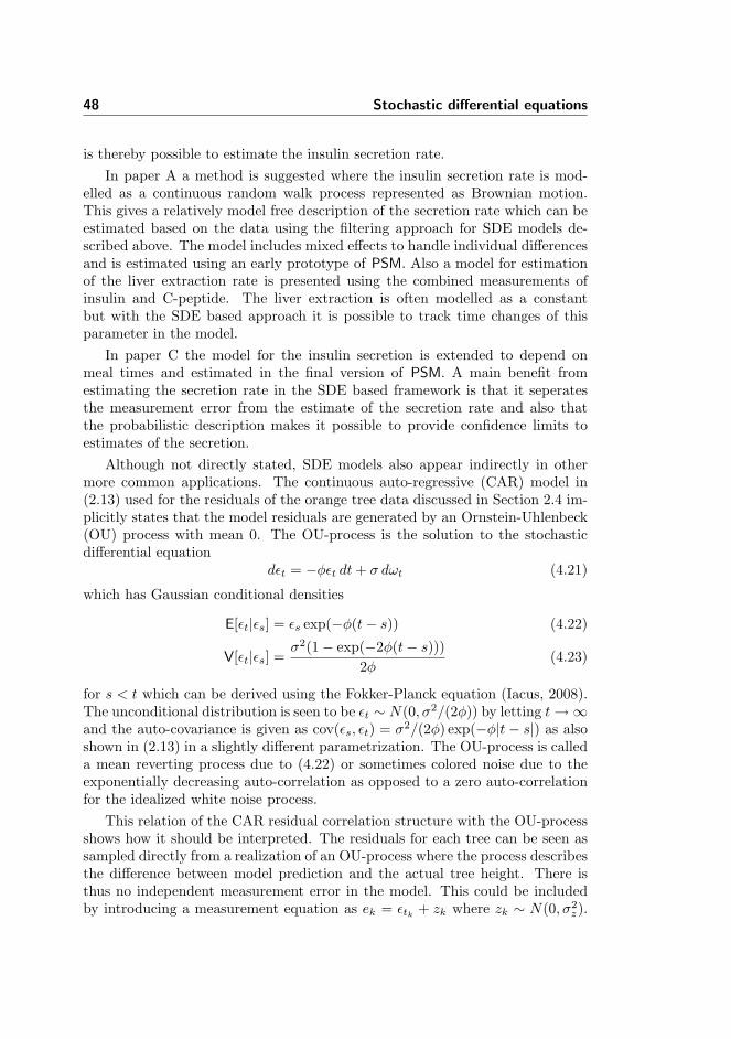
48 Stochastic differential equations
is thereby possible to estimate the insulin secretion rate.In paper A a method is suggested where the insulin secretion rate is mod-
elled as a continuous random walk process represented as Brownian motion.This gives a relatively model free description of the secretion rate which can beestimated based on the data using the filtering approach for SDE models de-scribed above. The model includes mixed effects to handle individual differencesand is estimated using an early prototype of PSM. Also a model for estimationof the liver extraction rate is presented using the combined measurements ofinsulin and C-peptide. The liver extraction is often modelled as a constantbut with the SDE based approach it is possible to track time changes of thisparameter in the model.
In paper C the model for the insulin secretion is extended to depend onmeal times and estimated in the final version of PSM. A main benefit fromestimating the secretion rate in the SDE based framework is that it seperatesthe measurement error from the estimate of the secretion rate and also thatthe probabilistic description makes it possible to provide confidence limits toestimates of the secretion.
Although not directly stated, SDE models also appear indirectly in othermore common applications. The continuous auto-regressive (CAR) model in(2.13) used for the residuals of the orange tree data discussed in Section 2.4 im-plicitly states that the model residuals are generated by an Ornstein-Uhlenbeck(OU) process with mean 0. The OU-process is the solution to the stochasticdifferential equation
dεt = −φεt dt+ σ dωt (4.21)
which has Gaussian conditional densities
E[εt|εs] = εs exp(−φ(t− s)) (4.22)
V[εt|εs] =σ2(1− exp(−2φ(t− s)))
2φ(4.23)
for s < t which can be derived using the Fokker-Planck equation (Iacus, 2008).The unconditional distribution is seen to be εt ∼ N(0, σ2/(2φ)) by letting t→∞and the auto-covariance is given as cov(εs, εt) = σ2/(2φ) exp(−φ|t− s|) as alsoshown in (2.13) in a slightly different parametrization. The OU-process is calleda mean reverting process due to (4.22) or sometimes colored noise due to theexponentially decreasing auto-correlation as opposed to a zero auto-correlationfor the idealized white noise process.
This relation of the CAR residual correlation structure with the OU-processshows how it should be interpreted. The residuals for each tree can be seen assampled directly from a realization of an OU-process where the process describesthe difference between model prediction and the actual tree height. There isthus no independent measurement error in the model. This could be includedby introducing a measurement equation as ek = εtk + zk where zk ∼ N(0, σ2
z).

4.6 Applications of SDE based models 49
The effect is that measurements taken at (almost) coinciding time points willnot have a correlation of 1 but instead only σ2/(σ2 + σ2
z). This is also called anugget-effect (Matheron, 1962) and can easily be included directly in the residualcorrelation structure in the NLMM by adding σ2
z to the diagonal in Σ in (2.5).

50 Stochastic differential equations

Chapter 5
Conclusion
A central part of the statistical methods used in this thesis are based on theMarkov property. Pharmacodynamic models can be described as hidden Markovprocesses in continuous state space by using stochastic differential equations tomodel random biological variations and fluctuations from unknown factors inthe system. Sleep processes based on a classification of sleep states can similarlybe modelled as a Markov process which instead evolves in a discrete state space.Although the response types in these two applications are fundamentally differ-ent the statistical models based on the Markov property show up as a strongmethod in both cases.
The work with pharmacodynamic models including SDEs in this project il-lustrates some of the benefits using this approach in comparisons to using modelssolely based on ODEs. In particular an application is presented which uses theSDE approach to estimate both insulin secretion and the liver extraction ratesof insulin for patients with type II diabetes. This is a powerful method madeavailable by SDEs that is generally applicable to estimation of unknown inputsor tracking of time varying parameters in both linear and nonlinear models.Today investigation of models based on SDEs within this area is mainly donefor research purposes, and this may to a large part be due to the lack of softwaresupporting estimation of SDE based models. This has been addressed duringthis project with the development of a software package (PSM) for this purpose,and the hope is that this will open up for an increased application of the SDEbased approach in the future within pharmacodynamic modelling.
Within sleep modelling a Markov based model has been used to model the
52 Conclusion
sleep hypnogram, which is the time series observations of sleep states. Thepresent work has focused on a continuous time representation which is arguedto give the most appropriate representation of the process, as sleep is known toevolve in continuous time. The main contribution within this area has been thedevelopment of a non-parametric estimation method which is able to give botha more robust and accurate estimate of the time variations of the parametersin the model compared to other more simple approaches. Being based on non-parametric methods makes it entirely data driven and it can thus be used to givevaluable detailed insight into the time dependence of the sleep process. Thiscan be used to establish a direct relation with sleep effect to the concentrationprofile of a drug, and thereby give an early indication of how the drug interactswith the body. This approach has been illustrated based on a sleep study in ratswhere both the PK profile and sleep effects have been considered in combination.
Both the Markov models for sleep and for pharmacodynamic models basedon SDEs can be used in a mixed modelling approach to handle variation be-tween groups in the data. If data has a crossed grouping structure (such as forindividuals belonging to different study centers) this poses a difficult estimationproblem which cannot easily be handled by standard software. It is proposedand demonstrated how such models instead can be estimated by a direct imple-mentation of the marginal likelihood function, which avoids these restrictionson the grouping structure for mixed modelling.
Bibliography
ADMB Project (2009). AD Model Builder Project. http://admb-project.org/.
Anderson, N. J., S. L. Garson, S. V. Fox, S. M. Doran, B. Ebert, and J. J.Renger (2006). SC & PO Gaboxadol cause dose-related increase in deltasleep without EEG hyper-synchrony. Society for Neuroscience. November2006 meeting. 157.30/V16.
Bates, D. M. and D. G. Watts (1988). Nonlinear Regression Analysis and ItsApplications. Wiley, New York.
Beal, S. and L. Sheiner (1980). The NONMEM System. The American Statis-tician 34, 118–119.
Beal, S. L. and L. B. Sheiner (2004). NONMEM R© Users Guide. NONMEMProject Group, University of California, San Francisco.
Bladt, M. and M. Sørensen (2005). Statistical inference for discretely ob-served markov jump processes. Journal of the Royal Statistical Society SeriesB 67 (3), 395–410.
Blume, J. and J. F. Peipert (2003). What your statistician never told youabout p-values. The Journal of the American Association of GynecologicLaparoscopists 10, 439–444.
Brodal, P. (2001). Sentralnervesystemet (3rd ed.). Oslo, Norway: Universitets-forlaget.
Cauter, E. V., F. Mestrez, J. Sturis, and K. S. Polonsky (1992). Estimationof insulin secretion rates from c-peptide levels. comparison of individual andstandard kinetic parameters for c-peptide clearance. Diabetes 41, 368–77.
54 BIBLIOGRAPHY
Cox, D. R. and H. D. Miller (1965). The Theory of Stochastic Processes.Methuen & Co Ltd.
Cuthbert, J. R. (1973). The logarithm function for finite-state markov semi-groups. Journal of the London Mathematical Society 6, 524–532.
Degn, K. B., C. B. Juhl, J. Sturis, G. Jakobsen, B. Brock, V. Chandramouli,J. Rungby, B. R. Landau, and O. Schmitz (2004). One Week’s Treatment Withthe Long-Acting Glucagon-Like Peptide 1 Derivative Liraglutide (NN2211)Markedly Improves 24-h Glycemia and alpha- and beta-Cell Function andReduces Endogenous Glucose Release in Patients with Type 2 Diabetes. Di-abetes 53, 1187–1194.
Diggle, P. J. (1988). An approach to the analysis of repeated measurements.Biometrics 44, 959–71.
Draper, N. R. and H. Smith (1981). Applied Regression Analysis (2nd ed.).Wiley, New York.
du Toit, S. H. C. and R. Cudeck (2009). Estimation of the nonlinear randomcoefficient model when some random effects are separable. Psychometrika 74,65–82.
Eaton, J. W. (2002). GNU Octave Manual. Network Theory Limited.
Elfving, G. (1937). Zur theorie der markoffschen ketten. Acta Societatis Scien-tiarum Fennicae A 2, 1–17.
Fan, J. and I. Gijbels (1996). Local Polynomial Modelling and Its Applications.Number 66 in Monographs on Statistics and Applied Probability. Chapman& Hall.
Forehand, C. J. (2003). Medical Physiology (2nd ed.)., Chapter 7, IntegrativeFunctions of the Nervous System. Lippincott Williams & Wilkins.
Gabrielsson, J. and D. Weiner (2006). Pharmacokinetic and PharmacodynamicData Analysis: Concepts and Applications (4th ed.). Kristianstads Boktryck-eri.
Gard, T. (1988). Introduction to Stochastic Differential Equations. New York:Marcel Dekker.
Goodman, S. N. (1999). Toward evidence-based medical statistics. 1: The pvalue fallacy. Annals of Internal Medicine 130, 995–1004.
Griewank, A. (2000). Evaluating derivatives: principles and techniques of algo-rithmic differentiation. Frontiers in applied mathematics. Philadelphia, PA:SIAM.

BIBLIOGRAPHY 55
Grube, G., A. Flexer, and G. Dorffner (2002). Unsupervised continuous sleepanalysis. Methods & Findings in Experimental & Clinical Pharmacology 24,51–56.
Himanen, S.-L. and J. Hasan (2000). Limitations of Rechtschaffen and Kales.Sleep Medicine Reviews 4, 149–167.
Himanen, S.-L., A. Saastamoinen, and J. Hasan (1999). Increasing the temporalresolution and stage specificity by visual adaptive scoring (vas) - a preliminarydescription. Sleep and Hypnosis 1, 22–28.
Iacus, S. M. (2008). Simulation and Inference for Stochastic Differential Equa-tions - With R Examples. Springer Series in Statistics. New York, USA:Springer.
Jazwinski, A. H. (1970). Stochastic Processes and Filtering Theory. New York,USA: Academic Press, Inc.
Kalman, R. E. (1960). A new approach to linear filtering and prediction prob-lems. Transactions of the ASME-Journal of Basic Engineering 82, 35–45.
Karlsson, M. O., R. C. Schoemaker, B. Kemp, A. F. Cohen, J. M. van Gerven,B. Tuk, C. C. Peck, and M. Danhof (2000). A pharmacodynamic markovmixed-effects model for the effect of temazepam on sleep. Clin PharmacolTher 68, 175–188.
Kemp, B. and H. A. C. Kamphuisen (1986). Simulation of human hypnogramsusing a markov chain model. Sleep 9, 405–414.
Kingman, J. F. C. (1962). The imbedding problem for finite markov chains. Z.Wahrscheinlichkeitstheorie 1, 14–24.
Kristensen, N. R. and H. Madsen (2003). Continuous time stochastic mod-elling - ctsm 2.3 mathematics guide. Technical report, Technical Universityof Denmark.
Lee, H. B. and M. D. Blaufox (1985). Blood volume in the rat. Journal ofNuclear Medicine 25, 72–76.
Lindstrom, M. J. and D. M. Bates (1990). Nonlinear mixed effects models forrepeated measures data. Biometrics 46, 673–687.
Madsen, H. (2008). Time Series Analysis (1st ed.). Texts in Statistical Science.Chapman & Hall/CRC.
Madsen, H., H. Spliid, and P. Thyregod (1985). Markov models in discrete andcontinuous time for hourly observations of cloud cover. Journal of AppliedMeteorology 24 (7), 629–639.

56 BIBLIOGRAPHY
Matheron, G. (1962). Traite de Geostatistique Appliquee, Volume I of Memoiresdu Bureau de Recherches Geologiques et Minieres. Paris: Editions Technip,Paris.
McCulloch, C. E. and S. R. Searle (2001). Generalized, Linear, and MixedModels. John Wiley & Sons, Inc.
Millar, R. B. (2004). Simulated maximum likelihood applied to non-gaussian andnonlinear mixed effects and state-space models. Australian & New ZealandJournal of Statistics 46, 543–554.
Moler, C. B. and C. F. Van Loan (1978). Nineteen dubious ways to computethe exponential of a matrix. SIAM Review 20, 801–836.
Nielsen, H. B. (2000). UCMINF - an algorithm for unconstrained, nonlinearoptimization. Technical Report IMM-REP-2000-19, Informatics and Mathe-matical Modelling (IMM), Technical University of Denmark.
Nielsen, H. B. and S. B. Mortensen (2008). ucminf: General-purpose uncon-strained non-linear optimization. R package version 1.0-6.
Nocedal, J. and S. J. Wright (2006). Numerical Optimization (2nd ed.). SpringerSeries in Operations Research. Springer.
Øksendal, B. (2007). Stochastic Differential Equations - An Introduction withApplications (6th ed.). Springer.
Pawitan, Y. (2001). In All Likelihood: modelling and inference using the likeli-hood. Oxford University Press.
Pinheiro, J. C. and D. M. Bates (1995). Approximations to the nonlinear mixed-effects model. Jounal of Computational and Graphical Statistics 4, 12–35.
Pinheiro, J. C., D. M. Bates, S. DebRoy, D. Sarkar, and the R Core team (2008).nlme: Linear and Nonlinear Mixed Effects Models. R package version 3.1-90.
R Development Core Team (2008). R: A Language and Environment for Statis-tical Computing. Vienna, Austria: R Foundation for Statistical Computing.ISBN 3-900051-07-0.
Rechtschaffen, A. and A. Kales (1968). A manual of standardized terminology,techniques and scoring system for sleep stages of human subjects. WashingtonDC.
Rowland, M. and T. N. Tozer (1997). Clinical Pharmacokinetics - Concepts andApplications (3rd ed.). Lippincott Williams & Wilkins.
Royall, R. (1997). Statistical evidence - A likelihood paradigm. Monographs onstatistics and applied probability 71. Chapman & Hall/CRC.
BIBLIOGRAPHY 57
SAS Institute Inc. (2004). SAS/Stat 9.1 User’s Guide. Cary, NC: SAS InstituteInc.
Sidje, R. B. (1998). Expokit. A software package for computing matrix expo-nentials. ACM Transactions on Mathematical Software 24 (1), 130–156.
Skaug, H. J. and D. A. Fournier (2006). Automatic approximation of themarginal likelihood in non-gaussian hierarchical models. ComputationalStatistics & Data Analysis 51, 699–709.
Tornøe, C. W., R. V. Overgaard, H. Agersø, H. A. Nielsen, H. Madsen, and E. N.Johnson (2005). Stochastic differential equations in NONMEM R©: Imple-mentation, application, and comparison with ordinary differential equations.Pharmaceutical Research 22, 1247–1258.
Turelli, M. (1977). Random environments and stochastic calculus. TheoreticalPopulation Biology 12, 140–178.
Vonesh, E. F. (1996). A note on the use of laplace’s approximation for nonlinearmixed-effects models. Biometrika 83, 447–52.
Wafford, K. A. and B. Ebert (2006). Gaboxadol – a new awakening in sleep.Current Opinion in Pharmacology 6, 30–36.
Walsh, J. K., S. Deacon, D.-J. Dijk, and J. Lundahl (2007). The selective ex-trasynaptic gabaa agonist, gaboxadol, improves traditional hypnotic efficacymeasures and enhances slow wave activity in a model of transient insomnia.Sleep 30, 593–602.
Wang, Y. (2007). Derivation of various NONMEM estimation methods. Journalof Pharmacokinetics and Pharmacodynamics 34, 575–593.
Ward, R. C. (1977). Numerical computation of the matrix exponential withaccuracy estimate. SIAM Journal on Numerical Analysis 14, 600–610.
Wolfinger, R. D. and X. Lin (1997). Two taylor-series approximation methodsfor nonlinear mixed models. Computational Statistics & Data Analysis 25,465–490.
Zung, W. W. K., T. H. Naylor, D. Gianturco, and W. P. Wilson (1965). AMarkov chain model of sleep EEG patterns. Electroencephalography and Clin-ical Neurophysiology 19, 105.

58 BIBLIOGRAPHY

Appendix A
Paper A
Title:A Matlab Framework for Estimation of NLME Models using Stochastic Differ-ential Equations: Applications for estimation of insulin secretion rates.
Authors:S. B. Mortensen, S. Klim, B. Dammann, N. R. Kristensen, H. Madsen, andR. V. Overgaard.
Published in:Journal of Pharmacokinetics and Pharmacodynamics 34, pp. 623-42 (2007).


J Pharmacokinet Pharmacodyn (2007) 34:623–642DOI 10.1007/s10928-007-9062-4
A matlab framework for estimation of NLME modelsusing stochastic differential equationsApplications for estimation of insulin secretion rates
Stig B. Mortensen · Søren Klim · BerndDammann · Niels R. Kristensen · HenrikMadsen · Rune V. Overgaard
Received: 17 November 2006 / Accepted: 27 April 2007 / Published online: 15 June 2007© Springer Science+Business Media, LLC 2007
Abstract The non-linear mixed-effects model based on stochastic differentialequations (SDEs) provides an attractive residual error model, that is able to handleserially correlated residuals typically arising from structural mis-specification of thetrue underlying model. The use of SDEs also opens up for new tools for model devel-opment and easily allows for tracking of unknown inputs and parameters over time. Analgorithm for maximum likelihood estimation of the model has earlier been proposed,and the present paper presents the first general implementation of this algorithm. Theimplementation is done in Matlab and also demonstrates the use of parallel computingfor improved estimation times. The use of the implementation is illustrated by twoexamples of application which focus on the ability of the model to estimate unknowninputs facilitated by the extension to SDEs. The first application is a deconvolution-type estimation of the insulin secretion rate based on a linear two-compartment modelfor C-peptide measurements. In the second application the model is extended to alsogive an estimate of the time varying liver extraction based on both C-peptide andinsulin measurements.
Keywords Non-linear mixed-effects modelling · SDE · Kalman smoothing ·Deconvolution · State-estimation · Parameter tracking · MatlabMPI · PK/PD
S. B. Mortensen (B)· S. Klim · B. Dammann · H. MadsenInformatics and Mathematical Modelling, Technical University of Denmark,Lyngby, Denmarke-mail: [email protected]
S. Klim · N. R. Kristensen · R. V. OvergaardNovo Nordisk A/S, Bagsvaerd, Denmark
123

624 J Pharmacokinet Pharmacodyn (2007) 34:623–642
Introduction
The non-linear mixed-effects (NLME) model based on ordinary differential equations(ODEs) is a widely used method for modelling pharmacokinetic/pharmacodynamic(PK/PD) data [1], since the model enables the variation to be split into inter- and intra-individual variation. It is, however, a well known problem that this model class has atoo restricted residual error structure, as it assumes that the residuals are uncorrelatedwhite noise. This assumption applies well to the expected distribution of assay error,but it is unfortunately a crude simplification to assume that the assumption also appliesto the remaining sources of error [2]. Other important sources of error may arise fromstructural model mis-specification or unpredictable random behavior of the underly-ing process, which both result in serially correlated residual errors. Previous workwith simulation of more complex error structures has shown that ignoring the serialcorrelation may lead to biased estimates of the variance components of the model orall population parameter estimates depending on the error structure [3].
A powerful way to deal with these problems is to introduce stochastic differentialequations (SDEs) in the model setup. SDEs are an extension to ODEs and facilitatethe ability to split the intra-individual error into two fundamentally different types:(1) serially uncorrelated measurement error, which is typically mainly caused byassay error and (2) system error, which may be caused by model mis-specifications,simplifications or true random behavior of the system.
Apart from providing a statistically more adequate model setup, the SDEs alsoallow new tools for the modeller. The SDE approach results in a quantitative estimateof the amount of system and measurement noise, and it can therefore also be used asa tool for model validation. If no significant system noise is found to be present, thisindicates that the proposed model structure gives a suitable description of the data.However, if significant system noise is found, it can be estimated and may be used toidentify a possible remaining model structure, since aspects which are not explicitlymodelled will give rise to system noise. It is important to emphasize that this rela-tion does not hold the other way around, since system noise may also arise from trueunmodellable random behavior of the system, and estimated system noise may thusnot be seen as evidence of an insufficient model structure. A detailed iterative schemefor model development based on SDEs has been described in [4]. Another importantadvantage of the SDE approach is the inherent confidence intervals for system states.This is facilitated by the estimation of system noise, and thus follows as a natural partof the model specification.
Several programs exist for modelling based on SDEs. The first implementationsfocused on single subject modelling, such as Continuous Time Stochastic Modelling(CTSM) [5]. CTSM is in fact also able to use multiple individuals for estimation ofstructural parameters, but this is done using a naive pooled likelihood function whereno inter-individual variance components are estimated. Later research has also madeit possible to include SDEs in population modelling by using an approximation algo-rithm of the likelihood function with SDEs for the widely used NLME model. Thisalgorithm is described in [6] and is based on the use of the Extended Kalman Filterto estimate conditional densities of each observation to form the individual likeli-hood function. The population likelihood function is then approximated based on the
123

J Pharmacokinet Pharmacodyn (2007) 34:623–642 625
first-order conditional estimation (FOCE) method. It has been shown in [7] how thisalgorithm for estimation of SDEs can be used in NONMEM [8], but this is by nomeans a trivial programming task to set up for a given model. It requires a modifieddata file and an implementation of the Kalman filter within the NONMEM controlstream. Moreover, the NONMEM implementation cannot be used to form Kalmansmoothing estimates, which is an important feature of the SDE approach, where alldata is used to give optimal estimates at each sampling point.
This paper will present the first prototype implementation of a general softwaretool for estimation of NLME models based on SDEs. The implementation has beenmade in Matlab and it makes experimentation with the new modelling approach read-ily available. The flexibility of the modelling approach will be demonstrated by twoexamples of applications. In the first example the model is used for stochastic decon-volution to estimate insulin secretion rates in 12 type II diabetic patients and in thesecond example the model is used to estimate/track the time variant behavior of theliver extraction rate for the same individuals.
Theory
This section contains an overview of the theory for population modelling using NLMEmodels based on SDEs. It will present the state space model for individual modellingand how this can be extended to incorporate SDEs. The parameters of the populationmodel are estimated with a maximum likelihood (ML) approach by first defining anindividual likelihood function, which forms the basis for the population likelihoodfunction. The individual likelihood function is evaluated on the basis of the ExtendedKalman Filter (EKF), and this will also be outlined. A more detailed description of theestimation algorithm can be found in [6]. To ease notation, all vectors and matricesare written using a bold font.
A mixed-effects model is used to describe data with the following general structure
yi j , i = 1, . . . , N , j = 1, . . . , ni (1)
where yi j is a vector of measurements at time ti j for individual i , N is the numberof individuals and ni is the number of measurements for individual i . Note that thenumber of measurements for each individual may vary. In a mixed-effects model thevariation is split into intra-individual variation and inter-individual variation, whichis modelled by a first and second stage model.
First stage model
The first stage model for an NLME model with ODEs can be written in the form of astate space model. A state space model consists of two parts, namely a set of continuousstate equations defining the dynamics of the system and a set of discrete measurementequations, which defines a functional relationship between the states of the system andthe measurements obtained. In the general form the state space equations are writtenas
123

626 J Pharmacokinet Pharmacodyn (2007) 34:623–642
dxt = f (xt , ut , t,φi )dt (2)
yi j = h(xi j , ui j , ti j ,φi ) + ei j (3)
where t is the continuous time variable and the states of the model and the optionalinputs at time t are denoted xt and ut respectively. The input ui j is typically frequentlysampled covariates such as body temperature etc. which may affect the system, or avariable indicating an interaction with the system such as an intravenous infusion. Boththe state, measurement and input can be multi-dimensional, and are in such cases thusrepresented by a vector at time ti j . The individual model parameters are denoted φiand finally f (·) and h(·) are the two possibly non-linear functions defining the model.Measurements are assumed observed with an uncorrelated Gaussian measurementerror. The variance of the error may depend on both state, input, time and individualparameters, that is ei j ∈ N (0,(xi j , ui j , ti j ,φi )).
It is important to draw attention to the concept of states, as this is essential to theunderstanding of the model setup. States are generally not directly observable or atbest only observable through measurement noise. The actual relation between mea-surements and states is defined in the measurement equation by the function h(·). Astate can represent many different aspects of the system of interest, e.g. concentra-tions or amounts in compartments, a volume, a parameter with unknown time varyingbehavior, or an input to the system that we wish to estimate. The state space formula-tion is thus a very flexible form of model specification, and the use of the state spacemodel will be illustrated with the applications presented later on in this paper.
Extending the first stage model with SDEs
In the ordinary state space model, noise is only allowed to enter through the measure-ment equation, see Eq. 3. The result is that error due to model mis-specification ortrue random fluctuations of the states is absorbed into the measurement error term andhence may give rise to correlated residuals. To allow for error to originate from thesystem specification, a stochastic term is added to the system equation. This results ina stochastic state space equation defined as follows
dxt = f (xt , ut , t,φi )dt + σω(ut , t,φi )dωt (4)
yi j = h(xi j , ui j , ti j ,φi ) + ei j (5)
where ωt is a standard Wiener process defined by ωt2 − ωt1 ∈ N (0, |t2 − t1|I). Theentire part σω(ut , t,φi )dωt is called the diffusion term and describes the stochasticpart of the system and f (xt , ut , t,φi )dt is called the drift term and describes the deter-ministic part. Together the drift and diffusion terms define the stochastic dynamics ofthe system.
By looking at the formulation of the extended first stage model, it is seen thatnoise is now allowed to enter in two places, namely as system noise via the diffusionterm and as measurement noise. It is noted that if no system noise is present, themodel will reduce into the standard ODE case, and this also ensures that physiologicalinterpretation of structural parameters is preserved with the use of an SDE model.
123

J Pharmacokinet Pharmacodyn (2007) 34:623–642 627
Second stage model
The second stage model for the individual parameters describes the variation of theindividual parameters φi between individuals and can be defined in a number of ways,each with different properties. In the present work it has been chosen to use
φi = g(θ, Zi ) · exp(ηi ) (6)
where ηi is the multivariate random effect parameter for the i th individual, which isassumed Gaussian distributed with mean zero and covariance :ηi ∈ N (0,). Thefixed effect parameter of the NLME model is θ , which is also sometimes referred toas the structural parameter or population parameter. The second stage model in Eq. 6includes an optional covariate Zi . This can be used to include individually measurablecovariates such as height, weight etc. that could affect φi . The chosen formulation ofthe 2nd stage model restricts variations in ηi from changing the sign of g(θ, Zi ) whichis typically an advantage as φi may be used as parameter for a variance or other sign-sensitive parameters. Moreover the resulting distribution of the individual parametersis log-Gaussian, as is often the case when dealing with PK/PD models. The secondstage model in Eq. 6 may easily be replaced if other model structures are needed,and this can be done without yielding any changes to the final population likelihoodfunction as long as ηi is still assumed to have a Gaussian distribution.
Maximum likelihood estimation of the NLME model with SDEs
The full set of parameters to be estimated for the final NLME model with SDEs are thematrices , σω, and the fixed effect parameters in the vector θ . The three matricesare usually fixed to some degree so that only the diagonals or other partial structureremains to be estimated.
The estimation of model parameters is based on a first stage likelihood function,which is formed as a product of probabilities for each measurement. Due to the assump-tion of correlated residuals with the inclusion of the Wiener process, it is necessary tocondition on the previous measurements to define the probability density of each mea-surement. In the approach chosen here, this is done by assuming that the conditionaldensities for the states are Gaussian and thus fully described by the state-predictionand the state prediction variance for each observation. These can be found using theExtended Kalman filter, which gives the unbiased minimum variance estimate of theevolution of the model states [9]. This will hold exactly for the linear case but only as anapproximation in the non-linear case. The assumptions for the EKF can be examinedby testing for a Gaussian distribution of the residuals and by testing for correctness ofthe estimated SDEs [10]. The prediction from the EKF is defined by
yi( j | j−1) = E( yi j |φi ,, σω, ui ,Yi( j−1)) (7)
Ri( j | j−1) = V ( yi j |φi ,, σω, ui ,Yi( j−1)) (8)
123

628 J Pharmacokinet Pharmacodyn (2007) 34:623–642
where Yi j = [ yi1, . . . , yi j ] and this gives the conditional distribution of the one-stepprediction error
εi j = yi j − yi( j | j−1) ∈ N (0, Ri( j | j−1)) (9)
The first stage likelihood function is calculated as the simultaneous density functionfor the i th individual
p1(Yini |φi ,, σω, ui ) =⎛⎝ ni∏
j=2
p(yi j |Yi( j−1), ·)⎞⎠ p(yi1|·) (10)
≈ni∏
j=1
exp(− 1
2εTi j R−1
i( j | j−1)εi j
)√|2π Ri( j | j−1)|
(11)
where conditioning on φi , , σω and ui is denoted “·”.Based on the first and second stage model density functions, the full NLME like-
lihood function can now be defined. The second stage distribution is simply a mul-tivariate Gaussian density denoted p2(ηi |), and combining this with the first stagedistribution results in the population likelihood function
L(θ ,, σω,) =N∏
i=1
∫p1(Yini |ηi , θ ,, σω, ui )p2(ηi |)dηi (12)
=N∏
i=1
∫exp(li )dηi (13)
where li is the a posteriori log-likelihood function for the random effects of the i thindividual given by
li = −1
2
ni∑j=1
(εT
i j R−1i( j | j−1)εi j + log |2π Ri( j | j−1)|
)− 1
2ηT
i −1ηi − 1
2log |2π|
(14)
The population likelihood function in Eq. 13 cannot be evaluated analytically, andtherefore li is approximated by a second-order Taylor expansion, where the expansionis made around the value ηi that maximizes li . At this optimum the first derivative∇li
∣∣ηi
= 0 and the population likelihood function therefore reduces to
L(θ ,, σω,) ≈N∏
i=1
∣∣∣∣−li2π
∣∣∣∣− 12
exp(li )∣∣∣ηi
(15)
as shown in Appendix. The approximation of the 2nd derivative li is done using theFOCE method, as it is also normally done in the NLME model based on ODEs. The
123

J Pharmacokinet Pharmacodyn (2007) 34:623–642 629
objective function for parameter estimation is chosen as the negative log-likelihoodfunction given as
− log L(θ ,, σω,) ≈N∑
i=1
(1
2log
∣∣∣∣−li2π
∣∣∣∣ − li
)(16)
Kalman filtering
The Extended Kalman Filter plays a central role for working with the NLME modelwith SDEs as seen from the previous section. Therefore a brief introduction to the EKFwill be given here, as well as to the three new types of state estimates made available.For a detailed description of the EKF algorithm please refer to [5,6,11,12].
For linear state-estimation problems the Kalman Filter will give an unbiased mini-mum variance state estimate. The solution can be derived explicitly using simple linearalgebra, and hence the algorithm runs efficiently in a computer implementation. Fornon-linear problems it is necessary to use another method for state-estimation likethat obtained by the Extended Kalman Filter, which has been used here. The ExtendedKalman Filter is for the main part identical to the Kalman Filter, except for the stateprediction which requires a solution to the non-linear differential system equations.This solution is obtained by a point-wise first-order approximation and therefore, fornon-linear systems, the EKF will only provide an approximate minimum variance esti-mate of the states. The EKF also runs slower due to the need for a numerical algorithmto solve the non-linear differential equations.
The Kalman Filter is a two-part algorithm consisting of prediction and updating,which iterates through all observations. In the prediction part the current estimatedstates and covariances are used to create predictions of the two first moments of the stateand observation to a time point ti j given the information at time ti( j−1). These predic-tions are denoted xi( j | j−1), P i( j | j−1), yi( j | j−1) and Ri( j | j−1), respectively. Updatingis performed at measurement time points, where the states and covariances are updatedaccordingly.
The updating is based on a compromise between the observation and current modelstate. In a situation where the model is good but the observations are dominated bymeasurement error, the state estimate should rely more on the model as opposed tofitting the observations. On the other hand, if the model is incomplete the states shouldrely more on the observations than the model. This trust in model versus observationsis balanced by the Kalman gain, which is dependent on the magnitude of system noiseσω and observation noise .
The initial conditions of the state and state covariance (xi(1|0) and P i(1|0)) need tobe specified for the Kalman filtering algorithm. The initial state can either be fixed orincluded in the likelihood function, whereas P i(1|0) for this implementation has beenchosen to be estimated as the integral of the Wiener process and system dynamics overthe first sample interval in accordance with the method used in [11].
A key feature of the SDE approach to population modelling is the ability to giveimproved estimates of the system states given the individual parameters and also to
123

630 J Pharmacokinet Pharmacodyn (2007) 34:623–642
provide confidence bands for the states. Confidence bands at a timepoint t are directlygiven by the estimated state covariance matrix P i(t |...) from the EKF, where t can beboth at or between measurements. There are four types of state and state covarianceestimates available when using the EKF, each of which differs in the way data is used.The four types are:
• Simulation estimate: xi( j |0), P i( j |0)
Provides an estimate of the state evolution for a repeated experiment, withoutupdating based on measurements. This is an ODE-like estimate, but it also yieldsa confidence band for the state evolution.
• Prediction estimate: xi( j | j−1), P i( j | j−1)
The prediction is used here to give the conditional density for the next observationat time ti j given the observations up to ti( j | j−1).
• Filtering estimate: xi( j | j), P i( j | j)
Best estimate at time ti j given the observations up to time ti j .
• Smoothing estimate: xi( j |N ), P i( j |N )
Optimal estimate at time ti j utilizing all observations both prior to and after timeti j .
For a conventional ODE model the state is found by the simulation estimate, whichis entirely given by the (possibly ML-estimated) initial state of the system. The covari-ance matrix for the states is 0 since no system noise is estimated. In other words theODE model assumes that a new experiment will yield an identical outcome of theunderlying system apart from observed measurement noise. By moving to SDEs, sys-tem noise is separated from measurement noise, thereby enabling the model to provideconfidence bands for the realization of the states in a new experiment. By improvingthe model, the confidence bands for the states will become narrower and theoreticallybe zero if the true model is used and no random fluctuations in system states arepresent.
With SDEs three new types of estimates, apart from the simulation estimate, alsobecome available. In the present setup the prediction estimate is used to give con-ditional Gaussian densities to form the likelihood function. The filter estimate is thebest obtainable state estimate during the experiment, where the subsequent observa-tions are not present. The third type of state estimate is the smoothed estimate. Thisprovides the optimal state and state covariance estimate (xi( j |N ) and P i( j |N )) basedon all obtained observations, both prior and subsequent to the time of interest. Thesmoothed estimate is therefore often the natural estimate of choice when studying thebehavior of the system in post hoc analysis.
Software implementation
The estimation algorithm outlined in the previous section has been implemented in aMatlab framework called population stochastic modelling (PSM). It is intended thatthis should work as a software prototype, in order to make further experimentation
123

J Pharmacokinet Pharmacodyn (2007) 34:623–642 631
with the model setup easily available. The program may be obtained by addressing anemail to the corresponding author.
Features
The implementation is designed to handle any non-linear mixed effects models usingSDEs based on the general model definition in the previous section. The model spec-ification is achieved through a set of Matlab functions written in m-files. A completemodel specification consists of state dynamics f and diffusion term magnitude σω,output function h and uncertainty , derivatives of state d f /dt and output dh/dt ,initial state x0, second stage model g and finally a variance function for the randomeffects. Each function is prepared to use all input arguments as specified by the modeldefinition.
The implementation has been made in two versions. The first is able to handle thegeneral non-linear case, and is thus based on the use of an algorithm for solving thedifferential equations in the EKF. It has been chosen to useode15s, which is a Matlabbuilt-in ODE solver. The second version is only able to solve linear systems, whichwill run significantly faster since it is based on an explicit solution of the differentialequations.
The population parameters are estimated by maximizing of the population likeli-hood function given in Eq. 15. Maximization is performed using a publicly availableMatlab implementation ucminf of a gradient search BFGS method with soft-linesearch and trust-region type monitoring of step length [13]. For additional perfor-mance it is possible to guide the optimization by providing an initial guess and bound-aries for the parameters. The implementation is also able to assess parameter varianceand correlation based on a numerical approximation of the Hessian of the likelihoodfunctions [14].
Implementation details
In the evaluation of the population likelihood function it is necessary to evaluate theindividual a posteriori log-likelihood function for each individual at its optimum,since a Taylor expansion is made around this point. Hence for one evaluation of thepopulation likelihood function an optimization must be performed on each individuallikelihood function. These optimizations only share the given population parametersand are therefore evaluated independently. This observation can be used to employthe use of parallel computing, where the individual optimizations are distributed to anumber of CPUs.
Matlab does not have the option for parallel computing by default1, but this can bemade possible using external software. MatlabMPI2 is a package developed at MITand it enables parallel computing in Matlab by creating a set of scripts that is executed
1 A distributed toolbox for Matlab is under development by The MathWorks.2 J. Kepner, Parallel Programming with MatlabMPI, http://www.ll.mit.edu/MatlabMPI/, 2006.
123

632 J Pharmacokinet Pharmacodyn (2007) 34:623–642
Table 1 Computation times using parallel computing
CPUs Time (s) Reduced to (%) CPU-time per individual (s) Overhead per CPU (%)
1 serial 241.8 100.0 12.1 −−1 242.4 100.2 12.1 0.2
2 128.3 53.0 12.8 5.8
3 101.7 42.0 15.3 20.7
4 72.0 29.7 14.4 16.0
5 66.0 27.3 16.5 26.7
10 50.0 20.6 25.0 51.6
in separate processes. MatlabMPI uses message passing but it was found faster to passall data and parameters through files. The individual calculation extracts its uniquepart of data by using its identifier number. The individual log-likelihood result ispassed back into the leader thread by proper message passing to avoid deadlocks orrace conditions. A shared memory environment is beneficial as message passing isimplemented through shared files.
In order to illustrate the effect of parallel computation for population modelling,a model was setup and estimated on the basis of simulated data for 20 subjects. Theresulting computation time is found in Table 1 and it can be seen that the computationtime is reduced to a little less than one-fifth of the original using five CPUs. For thisexample overhead begins to dominate when using more than five CPUs, however formore computationally intensive models, the benefit of adding more CPUs is expectedto be less affected by overhead.
For non-linear models a significant part of the computation time is spent in theprediction part of the Extended Kalman Filter when solving the differential systemequations. The prediction includes both state and state covariance, and these differen-tial equations are coupled and must therefore be solved simultaneously. To account forthis coupling, the two prediction equations have been collected into one system with acombined input vector Z which stores both the states and the covariance matrix. Thesymmetry in the covariance matrix is exploited so only the upper part is transferred,i.e.
Z =(
Z1Z2
)=
(xt |k
U (P t |k)
)(17)
where U () is a column vector containing the upper matrix. Conversion to the vectorZ is then used in conjunction with ode15s and the output is converted back into astate vector and covariance matrix. The use of a single vector Z complies with theMatlab standard conventions for ODE solving algorithms, and the chosen algorithmode15smay thus easily be substituted to suit the dynamic properties of a given model.
123
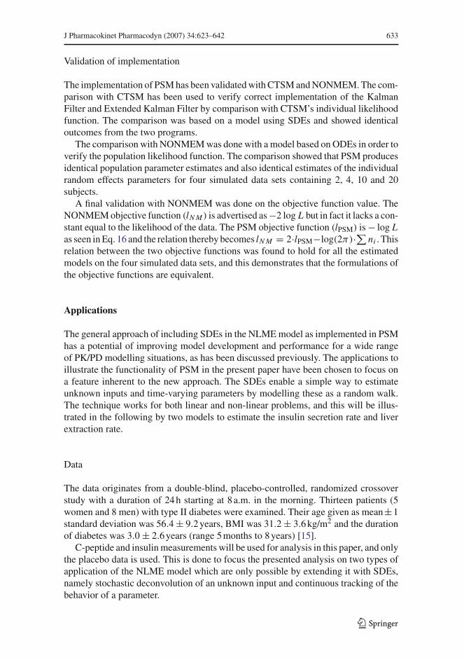
J Pharmacokinet Pharmacodyn (2007) 34:623–642 633
Validation of implementation
The implementation of PSM has been validated with CTSM and NONMEM. The com-parison with CTSM has been used to verify correct implementation of the KalmanFilter and Extended Kalman Filter by comparison with CTSM’s individual likelihoodfunction. The comparison was based on a model using SDEs and showed identicaloutcomes from the two programs.
The comparison with NONMEM was done with a model based on ODEs in order toverify the population likelihood function. The comparison showed that PSM producesidentical population parameter estimates and also identical estimates of the individualrandom effects parameters for four simulated data sets containing 2, 4, 10 and 20subjects.
A final validation with NONMEM was done on the objective function value. TheNONMEM objective function (lN M ) is advertised as −2 log L but in fact it lacks a con-stant equal to the likelihood of the data. The PSM objective function (lPSM) is − log Las seen in Eq. 16 and the relation thereby becomes lN M = 2·lPSM−log(2π)·∑ ni . Thisrelation between the two objective functions was found to hold for all the estimatedmodels on the four simulated data sets, and this demonstrates that the formulations ofthe objective functions are equivalent.
Applications
The general approach of including SDEs in the NLME model as implemented in PSMhas a potential of improving model development and performance for a wide rangeof PK/PD modelling situations, as has been discussed previously. The applications toillustrate the functionality of PSM in the present paper have been chosen to focus ona feature inherent to the new approach. The SDEs enable a simple way to estimateunknown inputs and time-varying parameters by modelling these as a random walk.The technique works for both linear and non-linear problems, and this will be illus-trated in the following by two models to estimate the insulin secretion rate and liverextraction rate.
Data
The data originates from a double-blind, placebo-controlled, randomized crossoverstudy with a duration of 24 h starting at 8 a.m. in the morning. Thirteen patients (5women and 8 men) with type II diabetes were examined. Their age given as mean±1standard deviation was 56.4 ± 9.2 years, BMI was 31.2 ± 3.6 kg/m2 and the durationof diabetes was 3.0 ± 2.6 years (range 5 months to 8 years) [15].
C-peptide and insulin measurements will be used for analysis in this paper, and onlythe placebo data is used. This is done to focus the presented analysis on two types ofapplication of the NLME model which are only possible by extending it with SDEs,namely stochastic deconvolution of an unknown input and continuous tracking of thebehavior of a parameter.
123
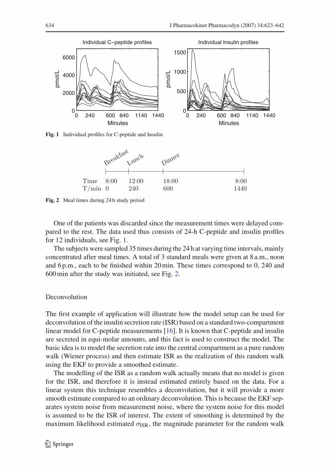
634 J Pharmacokinet Pharmacodyn (2007) 34:623–642
0 240 600 840 1140 14400
2000
4000
6000
Individual C−peptide profiles
pmol
/L
Minutes0 240 600 840 1140 1440
0
500
1000
1500
Individual Insulin profiles
pmol
/L
Minutes
Fig. 1 Individual profiles for C-peptide and Insulin
Breakfa
st
Lunch
Dinner
TimeT/min
8:008:00 12:00 18:000 240 600 1440
Fig. 2 Meal times during 24 h study period
One of the patients was discarded since the measurement times were delayed com-pared to the rest. The data used thus consists of 24-h C-peptide and insulin profilesfor 12 individuals, see Fig. 1.
The subjects were sampled 35 times during the 24 h at varying time intervals, mainlyconcentrated after meal times. A total of 3 standard meals were given at 8 a.m., noonand 6 p.m., each to be finished within 20 min. These times correspond to 0, 240 and600 min after the study was initiated, see Fig. 2.
Deconvolution
The first example of application will illustrate how the model setup can be used fordeconvolution of the insulin secretion rate (ISR) based on a standard two-compartmentlinear model for C-peptide measurements [16]. It is known that C-peptide and insulinare secreted in equi-molar amounts, and this fact is used to construct the model. Thebasic idea is to model the secretion rate into the central compartment as a pure randomwalk (Wiener process) and then estimate ISR as the realization of this random walkusing the EKF to provide a smoothed estimate.
The modelling of the ISR as a random walk actually means that no model is givenfor the ISR, and therefore it is instead estimated entirely based on the data. For alinear system this technique resembles a deconvolution, but it will provide a moresmooth estimate compared to an ordinary deconvolution. This is because the EKF sep-arates system noise from measurement noise, where the system noise for this modelis assumed to be the ISR of interest. The extent of smoothing is determined by themaximum likelihood estimated σISR, the magnitude parameter for the random walk
123

J Pharmacokinet Pharmacodyn (2007) 34:623–642 635
k
k
CC
ISR
k
1
1
2
2
e
Fig. 3 Two-compartment model used for estimation of ISR
0 240 600 840 1140 14400
100
200
pmol
/L
ISR
± SD
0 240 600 840 1140 14400
100
200
pmol
/L
Time (min)
Fig. 4 Smoothed estimate of ISR for individual 1 and 2
for ISR, which influences the Kalman gain on increments of the random walk. A largermagnitude leads to a more fluctuating random walk with larger increments and viceversa for a smaller magnitude. The resulting estimate of the random walk and therebythe ISR is thus optimal in a likelihood sense, since the EKF as mentioned earlier hasbeen shown to yield the minimum variance state estimate for a linear system.
The deconvolution setup requires three states, namely a central compartment stateC1 modelling the measured C-peptide concentration, a peripheral compartment stateC2, and a state ISR for the random walk. This gives the state vector x = [ C1 C2 ISR ]T .The C-peptide kinetic parameters k1, k2, ke are set equal to the Van Cauter estimatesfound in [17].
The C-peptide measurement error is assumed to be additive Gaussian white noisewith variance . The model states are constrained to steady state at t = 0 given an
initial individually estimated concentration Ci in C1, that is x0 = [Ci
k1k2 Ci keCi
]T
and Ci = C01 exp η, η ∈ N (0,C1). The state equation for the model is shown in
Eq. 18
dx =⎡⎣−(k1 + ke) k2 1
k1 −k2 00 0 0
⎤⎦ x dt + diag
⎡⎣ 00
σISR
⎤⎦ dω (18)
and the measurement equation is simply y = C1 + ε, where ε ∈ N (0, ). TheML estimated population parameters are C0
1 , , σISR and C01
and based on these anoptimal estimate of ISR can be found by using the Kalman smoothing algorithm.
123

636 J Pharmacokinet Pharmacodyn (2007) 34:623–642
Pancreas
ISR
Liver
F · ISR
I C1 C2
ke ke,I
k1
k2
Fig. 5 Dynamics of the combined model for estimation of insulin secretion rate and liver extraction rate
Figure 4 shows the smoothed estimate of ISR for the first two individuals togetherwith a ±1 standard deviation band. The assumption of steady state in the beginningdefines the initial level of ISR based on C0
1 and this appears appropriate.
State-estimation
The second example of application goes to illustrate how the model setup may be usedfor state-estimation in non-linear systems. The method is also sometimes referred toas parameter tracking, when the state represents a parameter, which is suspected ofhaving some time-varying behavior. Although non-linear state-estimation is funda-mentally different from deconvolution, which only applies to linear systems, it can beperformed with SDEs in basically the same way as the approach for deconvolutionpresented in the first example of application.
The aim is to estimate the dynamic liver extraction rate, which represents the frac-tion of insulin that is absorbed by the liver. This fraction is often modelled as a constantto simplify statistical models, although it is known to be time-varying. As previouslydone the insulin secretion rate is estimated based on the information in the C-peptidemeasurements and then used as input into a one-compartment insulin model. The stateI models the measured insulin concentration in the compartment and the insulin elim-ination is set to ke,I = 0.355 min−1. This value has been reported for a similar study,also on type II diabetic patients [18]. By having a fixed elimination rate and ISR givenfrom the C-peptide part of the data, the information in the insulin measurement canbe used to estimate the liver extraction. The fraction which passes through the liveris modelled by a state F , and the input into the insulin compartment is thus F · ISRmaking the model non-linear in the states. The final layout of the model is shown inFig. 5. The layout is identical to the layout first proposed in [19], where it is shownthat by assuming a constant liver extraction rate it is possible to estimate the kineticparameters and a piecewise constant ISR.
In an initial model F was modelled directly as a random walk in the same way as ISR.The estimation of the model returned a very low estimate of the insulin measurement
123

J Pharmacokinet Pharmacodyn (2007) 34:623–642 637
standard deviation at only 0.01 pmol/l. This is an unrealistically small value and indi-cates a problem with separation of noise components, since virtually all the variationin the insulin measurements thereby is assumed to originate from the fluctuations ofthe liver extraction.
This problem can be solved by imposing further smoothing to the state-estimationby choosing to model the derivative of F as a random walk instead of directly F asbefore. This is achieved by introducing a new state named X as shown in Eq. 19 and20
d F
dt= X (19)
d X = σX dω (20)
where ω is a Wiener process. The change in the model for F causes the increments ofthe derivative of F to be penalized by the Wiener noise gain σ instead of the incre-ments of F directly. The result is a less flexible model for F where fluctuations arefurther constrained, and the modification is easily implemented using the flexibilitymade available by the stochastic state space approach. In total the model contains sixstates, namely x = [C1 C2 I ISR F X ]T , which are all estimated simultaneously bythe Extended Kalman Filter using the two-dimensional measurements with C-peptideand insulin. The system equations are shown in Eq. 21.
dx =
⎡⎢⎢⎢⎢⎢⎢⎣−(k1 + ke)C1 + k2C2 + I S Rk1C1 − k2C2−ke,I I + F · I S R0X0
⎤⎥⎥⎥⎥⎥⎥⎦ dt + diag
⎡⎢⎢⎢⎢⎢⎢⎣000
σISR0
σX
⎤⎥⎥⎥⎥⎥⎥⎦ dω (21)
The estimation of the population parameters in the new model with a constrainedmodel for F results in a better separation of noise. The standard deviation for theinsulin secretion rate is estimated at a satisfactory level of 19.8pmol/l.
As could be expected, the model finds an ISR which is almost identical to the onefound using just a C-peptide deconvolution model, since the information in the addedinsulin measurements is used to estimate the liver extraction. The smoothed estimateof the fraction of insulin passing the liver F is shown in Fig. 6 for individual 1 and 2.The plots illustrate that the proportion sent through the liver, F , is below one for theentire time interval as it naturally should be. This also holds for 8 out of the remaining10 individuals. For the two last individuals F varies between 0.5 and 1.8. This ishowever not of great concern, because F and ke,I are correlated and it is thus probablyjust indicating that ke,I for this particular individual is set too high.
123

638 J Pharmacokinet Pharmacodyn (2007) 34:623–642
0 240 600 840 1140 14400
0.5
1
0 240 600 840 1140 14400
0.5
1
Time(min)
Fig. 6 Smoothed fraction of insulin passing the liver ±1 SD for individual 1 and 2
Discussion
By the presented software implementation PSM, we have shown that it is possible todevelop a general purpose PK/PD population modelling tool that is able to handle theextra functionality made available by using SDEs in NLME models. The implemen-tation opens up for the possibility to easily make further experiments with the modelsetup to allow for accumulation of more knowledge about the modelling approach.
It is important to emphasize that the software implementation is to be considereda prototype, which should only be used on research level. A necessary step to make itmore widely usable is to move to another programming language. This implementationhas been done in Matlab, which is ideal for numerical implementations, but it lacksin speed and parallel computing options. The standard within scientific programmingtoday is Fortran, and this is also an obvious choice here due to its efficient handlingof numerical computations and linear algebra calculations. Another advantage of For-tran is the accessibility of modules already available, such as algorithms for numericaloptimization and ODE solvers.
The optimal platform for a future implementation is a shared memory system.Shared memory parallelism can be implemented easily in Fortran using the OpenMP3
application program interface. OpenMP supports multi-platform shared-memory par-allel programming in Fortran on all architectures, including Unix and Windows plat-forms. OpenMP is a scalable model that gives a flexible interface for developing aparallel application for platforms ranging from the desktop to the supercomputer andit supports parallelism through meta tags that will make portability to single CPU,multi-core CPU, and shared-memory multiprocessor (SMP) units simple. Some com-pilers are also able to create parallel calculations by automatically analyzing the code,but the largest improvements are achieved using manual parallelization.
3 Further details may be found at www.openmp.org.
123

J Pharmacokinet Pharmacodyn (2007) 34:623–642 639
The present paper has illustrated how parallelization introduced at the individualminimizations of the population likelihood function has a strong potential of reducingthe estimation time for a future final software program when dealing with data con-taining a large number of individuals. It can also be argued to introduce parallelism atan even higher level in the gradient calculation of the population likelihood function.This would generally be advantageous for models where the number of populationparameters exceeds the number of individuals in data.
The first example of application in this paper demonstrated how the NLME modelcan be used for deconvolution of ISR by introducing SDEs. Although the estimationof ISR using SDEs is loosely denoted deconvolution, it is in fact not strictly speakingdeconvolution but instead a probabilistic description of an unknown input, which ismodelled as the realization of a stochastic process. Pure deterministic deconvolutionusing ODEs for the model shown in Fig. 3 will estimate ISR at each measurement tobe equal to the rate giving the ‘missing’ amount in the central C-peptide compartmentC1. With the SDE approach the measurement noise on C-peptide is taken into accountby the Kalman filter, which yields a minimal variance estimate of the states resultingin a more smooth estimate of ISR where the effect of noise is reduced.
Deconvolution based on noisy data is generally an ill-posed problem, meaning thateven small perturbations in data lead to significant changes in the estimated solution[20]. The problem has been addressed by existing software by applying various kindsof regularization techniques to constrain the solution. An example is WinNonlin [21],which is a standard PK/PD software solution that can also be used for deconvolution.The program addresses the problem of deconvolution by introducing a smoothnessfactor and as a consequence it is simply left up to personal choice and preference ofthe user to specify the level of smoothing. An improved solution can be found usingWinStoDec presented by [22], which is based on stochastic deconvolution and canbe used for linear time-invariant systems [23]. It has been shown by [24] that thestochastic deconvolution approach is equivalent to the SDE approach presented here,which is furthermore by nature also able to handle non-linear time-varying systems,as has been demonstrated with the state-estimation approach in the second exampleof application presented here.
In conclusion, a fully functional prototype tool named PSM for estimation of NLMEmodels based on SDEs has been implemented in Matlab and validated. The use of par-allelization in the implementation has demonstrated a strong potential of reducing com-putation times in future implementations in a faster programming language. Finallytwo examples of application concerning insulin modelling demonstrated the possibil-ity for deconvolution and non-linear parameter tracking facilitated by the extensionof the NLME model to use SDEs.
Acknowledgments
The Authors wish to thank Ole Schmitz MD and his co-workers at The Institute ofPharmacology, University of Aarhus, for conducting the present study enabling us toperform the presented analysis.
123

640 J Pharmacokinet Pharmacodyn (2007) 34:623–642
Appendix: Approximation of population likelihood function
The population likelihood function for the NLME model with SDE’s is defined in Eq.13 as
L(θ ,, σω,) =N∏
i=1
∫exp(li )dηi (22)
where li is the individual a posteriori log-likelihood function. In most cases the integralcannot be evaluated analytically. For a general evaluation the individual a posteriorilikelihood function can be approximated by a second order Taylor series expansion ofli around the value ηi of the individual random effects parameter which maximizes li .It follows that
li ≈ li + ∇T li (ηi − ηi ) + 1
2(ηi − ηi )
T li (ηi − ηi ) (23)
≈ li + 1
2(ηi − ηi )
T li (ηi − ηi ) (24)
since ∇li = 0 at ηi . Based on the approximation in Eq. 24 the integral in Eq. 22 cannow be evaluated by moving constants such that the integral is over a multi-variateGaussian density with mean ηi and variance (−li )−1. This integral is equal to oneand the result is
∫Li dηi ≈
∫Li · exp
(−1
2(ηi − ηi )
T (−li )(ηi − ηi )
)dηi (25)
≈ Li
∣∣∣∣ 2π
−li
∣∣∣∣ 12∫ ∣∣∣∣ 2π
−li
∣∣∣∣− 12
exp
(−1
2(ηi − ηi )
T (−li )(ηi − ηi )
)dηi
(26)
≈ Li
∣∣∣∣ 2π
−li
∣∣∣∣ 12 · 1 (27)
≈ Li
∣∣∣∣−li2π
∣∣∣∣− 12
(28)
where Li = exp(li ). The step in Eq. 28 is done to avoid a matrix inversion of theHessian. By combining Eq. 22 Eq. 28 the population log-likelihood function can nowbe approximated by
L(θ,, σω,) ≈N∏
i=1
∣∣∣∣−li2π
∣∣∣∣− 12
exp(li )∣∣∣ηi
. (29)
123
J Pharmacokinet Pharmacodyn (2007) 34:623–642 641
References
1. Aarons L (1999) Editorial–pharmacokinetic and pharmacodynamic modelling in drug development.Stat Methods Med Res 8(3): 181–182
2. Karlsson MO, Jonsson EN, Wiltse CG, Wade JR (1988) Assumption testing in population phar-macokinetic models: Illustrated with an analysis of moxonidine data from congestive heart failurepatients. J Pharmacokinet Biopharm 26(2): 207–246
3. Karlsson MO, Beal SL, Sheiner LB (1995) Three new residual error models for population pk/pdanalyses. J Pharmacokinet Pharmacodyn 23(6): 651–672
4. Kristensen NR, Madsen H, Ingwersen SH (2005) Using stochastic differential equations for pk/pdmodel development. J Pharmacokinet Pharmacodyn 32:109–141
5. Kristensen NR, Madsen H, Jørgensen SB (2004) Parameter estimation in stochastic grey-box mod-els. Automatica 40: 225–237
6. Overgaard RV, Jonsson N, Tornøe CW, Madsen H (2005) Non-linear mixed-effects models withstochastic differential equations: implementation of an estimation algorithm. J of PharmacokinetPharmacodyn 32(1): 85–107
7. Tornøe CW, Overgaard RV, Agersø H, Nielsen HA, Madsen H, Johnson EN (2005) Stochastic differ-ential equations in nonmem®: Implementation application and comparison with ordinary differentialequations. Pharm Res 22(8): 1247–1258
8. Beal SL, Sheiner LB (2004) NONMEM®users guide. University of California, NONMEM ProjectGroup
9. Kalman RE, Bucy RS (1961) New results in linear filtering and prediction theory. Trans ASME SerD J Basic Engrg 83: 95–108
10. Holst J, Lindström E, Madsen H, Nielsen HA (2000) Model validation in non-linear continuous-dis-crete grey-box models. Proceedings of the 13th IFAC symposium on system identification RotterdamThe Netherlands
11. Kristensen NR, Madsen H (2003) Continuous time stochastic modelling-ctsm 2.3 mathematicsguide. Technical report Technical University of Denmark December
12. Gelb A, Kasper JF Jr, Nash RA Jr, Price CF, Sutherland AA Jr (1982) Applied Optimal Estimation.The MIT Press seventh edition
13. Nielsen HB (2000) Ucminf–an algorithm for unconstrained nonlinear optimization. Technical reportIMM DTU
14. Dennis JE Jr, Schnabel RB (1983) Numerical methods for unconstrained optimization and nonlinearequations. Prentice Hall Series in Computational Mathematics, Prentice Hall Inc.
15. Degn KB, Juhl CB, Sturis J, Jakobsen G, Brock B, Chandramouli V, Rungby J, Landau BR, SchmitzO (2004) One week’s treatment With the long-acting glucagon-Like peptide 1 derivative liraglu-tide (NN2211) markedly improves 24-h glycemia and alpha- and beta-Cell function and reducesendogenous glucose release in patients with type 2 diabetes. Diabetes 53(5): 1187–1194
16. Gabrielsson J, Weiner D (1997) Pharmacokinetic and pharmacodynamic data analysis: conceptsand applications. Kristianstads Boktryckeri second edition
17. Van Cauter E, Mestrez F, Sturis J, Polonsky KS (1992) Estimation of insulin secretion rates fromc-peptide levels. comparison of individual and standard kinetic parameters for C-peptide clearance.Diabetes 41(3):368–377
18. Kjems LL, Vølund A, Madsbad S (2001) Quantification of beta-cell function during ivgtt in type iiand non-diabetic subjects: assessment of insulin secretion by mathematical methods. Diabetologia44: 1339–1348
19. Watanabe RM, Steil GM, Bergman RN (1998) Critical evaluation of the combined model approachfor estimation of prehepatic insulin secretion. Am J Physiol 274(1): 172–183
20. Hadamard J (1923) Lectures on the Cauchy problem in linear partial differential equations. YaleUniversity Press New Haven
21. Pharsight (2004) WinNonlin user manual version 3.1. Pharsight deconvolution edition22. Sparacino G, Pillonetto G, Capello M, Nicolao G , De Cobelli C (2002) Winstodec: a stochastic de-
convolution interactive program for physiological and pharmacokinetic systems. Comput MethodsPrograms Biomed 67: 67–77
123

642 J Pharmacokinet Pharmacodyn (2007) 34:623–642
23. de Nicolao G, Sparacino G, Cobelli C (1997) Nonparametric input estimation in physiological sys-tems: problems methods and case studies. Automatica 33(5): 851–870
24. Kristensen NR, Madsen H, Ingwersen SH (2004) A deconvolution method for linear and nonlinearsystems based on stochastic differential equations. poster presented at: population approach groupin Europe (PAGE) 13th meeting June
123

80 Paper A
Appendix B
Paper B
Title:Introduction to PK/PD modelling with focus on PK and stochastic differentialequations.
Authors:S. B. Mortensen, A. H. Jonsdottır, S. Klim, and H. Madsen.
Published in:IMM-Technical Report-2008-16 (2008).

Introduction to PK/PD modellingwith focus on PK and stochastic differential equations
Stig Mortensen, Anna Helga Jonsdottir,Søren Klim and Henrik Madsen
June 23, 2009
DTU Informatics
DTU InformaticsDepartment of Informatics and Mathematical ModelingTechnical University of Denmark
Richard Petersens PladsDTU - building 321DK-2800 Kgs. LyngbyDenmark
ISSN: 0601-2321

Contents
1 Introduction 2
2 The ADME Model 3
3 Fundamental concepts 4
4 Compartment models 54.1 One-compartment models . . . . . . . . . . . . . . . . . . . . . . 7
4.1.1 Case study: pain reliever . . . . . . . . . . . . . . . . . . 84.1.2 Flip-flop situation . . . . . . . . . . . . . . . . . . . . . . 104.1.3 Maximum concentration . . . . . . . . . . . . . . . . . . . 114.1.4 Half-life of drug . . . . . . . . . . . . . . . . . . . . . . . . 114.1.5 Constant rate infusion and multiple dosing . . . . . . . . 12
4.2 Multi-compartment models . . . . . . . . . . . . . . . . . . . . . 134.2.1 Case study: pain reliever continued . . . . . . . . . . . . . 15
5 PD modelling 155.1 Receptor Theory . . . . . . . . . . . . . . . . . . . . . . . . . . . 16
5.1.1 Michaelis-Menten model . . . . . . . . . . . . . . . . . . . 175.1.2 Commonly used PD models . . . . . . . . . . . . . . . . . 18
5.2 Modelling with effect compartments . . . . . . . . . . . . . . . . 195.2.1 Case study: pain reliever continued . . . . . . . . . . . . . 20
6 Modelling data 226.1 Single individual . . . . . . . . . . . . . . . . . . . . . . . . . . . 22
6.1.1 Error model using ODEs . . . . . . . . . . . . . . . . . . 226.1.2 Error model using SDEs . . . . . . . . . . . . . . . . . . . 256.1.3 Case study: Advantages of using SDEs . . . . . . . . . . . 276.1.4 Discussion of SDEs . . . . . . . . . . . . . . . . . . . . . . 30
6.2 Multiple individuals . . . . . . . . . . . . . . . . . . . . . . . . . 316.3 Estimation . . . . . . . . . . . . . . . . . . . . . . . . . . . . . . 32
6.3.1 NONMEM . . . . . . . . . . . . . . . . . . . . . . . . . . 326.3.2 CTSM . . . . . . . . . . . . . . . . . . . . . . . . . . . . . 336.3.3 PSM . . . . . . . . . . . . . . . . . . . . . . . . . . . . . . 33
A NLME log-likelihood function 33
1

1 Introduction
The development of new medical drugs is driven by progress in many areas.These include medicine, biotechnology, new production equipment and not least,as will be the focus here, the area of mathematical and statistical modelling.
Before a new drug can move from a simple molecule in the laboratory tobecome a new product in the local pharmacy, there are many questions whichmust first be answered: Is it safe, also for patients, elderly people, pregnantwomen, etc.? Does the drug work? In which way should it be given to thepatient? Are there any unwanted side-effects? The answer to all these questionsrequire a long series of trials, which must be carefully planned to discover allfacets of a new drug candidate.
New drug candidates are in the early development phase initially tested withanimals. These tests aim to show if the drug seems to work and also to check forunwanted side effects. The next step is to move to clinical trials with humans.These trials have traditionally been separated into 4 phases. In Phase 1 the drugis given to healthy young male persons mainly to see if it is safe for humansbut the sponsor (the drug company) will of course also look for indications of apositive effect. In Phase 2 the drug is given to the target patient group againmainly to show that it is still safe, but also to give indications of a positiveeffect. When safety has been established and the sponsor believes in the drugspotential, it will be moved to Phase 3, which generally involve the largest andmost costly trials. These trials focus on proving the positive effect of the drugto the health authorities. If all goes well, the drug is approved and marketed.In some cases this will be followed by new trials, which is known as Phase 4studies.
The series of clinical trials is not only very costly but also time consuming.The drug may easily take 10 years to get approved and marketed to the patients.Due to this both health authorities and drug companies are looking of ways toaccelerate this project, while still keeping it as safe as possible. The primarytarget is to insure that no harmful drugs get approved, but at the same timethat the good drug are not delayed unnecessarily from reaching the patients,who will benefit from them. It is in this connection that mathematical andstatistical modelling has become an important tool, since it may help to giveimproved understanding of the outcome of clinical trials.
The scientific disciplines concerning mathematical modelling in drug devel-opment are called pharmacokinetics and pharmacodynamics, or in brief justPK/PD. In popular terms PK is often described as “what the body does tothe drug” and PD as “what the drug does to the body”. More specificallyPK focuses on modelling how the drug passes through the body, normally bymodelling concentrations in various areas of the body as a function of time, seeFigure 1(a). PD aims at linking these modelled drug concentration to certain
2

measure of effect through a PD-model. An example of a PD-model is shownin Figure 1(b). With a combined PK/PD model it is thus possible to give apicture of the expected effect for a given dose as a function of time as illustratedin Figure 1(c).
Time
Con
cent
ratio
n
(a) PK model
Concentration
Effe
ct
(b) PD model
Time
Effe
ct
(c) Combined PK/PD model
Figure 1: Illustration of PK/PD modelling.
For more thorough reading on pharmacokinetics and pharmacodynamics thebooks Gabrielsson and Weiner (1997) and Rowland and Tozer (1997) are sug-gested.
2 The ADME Model
A complicated process is initiated as soon as a drug enters the body. Thisprocess can be divided into four phases, absorption, distribution, metabolismand elimination and hence the acronym ADME.
The absorption phase describes how the drug enters the body, or more pre-cisely how the drug enters the bloodstream. When using intravenous (iv) ad-ministration, no absorption phase is present since the drug is injected directlyinto the bloodstream. The whole dose can be given in one rapid injection, calleda bolus dose, or by using a constant rate infusion over a certain period of time.All other dosing methods, that is when the drug is not injected directly into
3

the bloodstream, are called extravascular dosing. Examples of such methodsare injections into a muscle or fat tissue and oral dosing. Those methods haveone thing in common, they require an absorption phase since the drug needsto cross some boundaries in the body before it reaches the bloodstream. As anexample when administrating a pill (oral dosing), the pill needs to dissolve andcross the gut wall before it reaches the bloodstream.
The distribution phase describes how the drug spreads through the body,into its fluids and tissues, after it has reached the bloodstream. It is in thedistribution phase the drug is brought to the place of action trough the blood-stream. The time it takes for the drug to get to the place of action is verydependent on if it is easily accessible by the bloodstream. The heart is, as anexample, easily accessible by the bloodstream while the bone marrow is not.
The third phase, metabolism, describes a process where the initial (parent)compound is broken into another compounds, called metabolites. The metabo-lites can either be inactive, therefore reducing the drugs effect on the body, orthey can be active, sometimes more active than the parent compound. The liverplays a leading role in metabolism since it produces many of the enzymes usedby metabolism.
The last phase, the elimination phase, describes how the compounds andtheir metabolites are removed from the body via excretion. Most drugs areeliminated via the kidneys with urine.
The four phases of the ADME model can be summarized as:
Absorption Drug entering the body
Distribution Drug is spreading to different areas of the body
Metabolism Drug is being changed to new chemical compounds
Elimination Drug is removed from the body
3 Fundamental concepts
Concentration is defined as amount per volume and is the most central conceptin PK/PD modelling. The reason is that concentration of a drug is relativelyeasy to measure from a blood sample and at the same time concentration is akey factor when modelling both positive and negative effects of a drug. Con-centration is calculated as
C =A
V(1)
4

where A is amount of drug and V is the volume of distribution. The amountof drug is either measured as mass (mg) or in number of molecules (mol). Thevolume of distribution is defined as the volume which the drug has to distributeevenly into in order to reach the measured concentration in the blood, C. If thethe drug only distributes into the blood then the volume of distribution will beequal to the volume of the blood. However, often the volume of distribution willbe larger than the volume of the blood. This can happen if the drug distributesinto other parts of the body or if the drug is chemically bound in a way where itcannot be measured. The amount of drug is unchanged, but only a smaller partcan be measured in the blood. This will result in a larger volume of distributionto reflect the lower measured concentration of the drug.
Another central issue is the timecourse of the elimination of the drug. In themost simple model one assumes that the elimination rate is proportional to theremaining amount of drug, A. The proportionality constant is CL/V , whereCL is called clearance and measures the volume of blood which is cleared fordrug per time. The rate of clearance is thus CL/V ·A. CL and V are sometimesreferred to as micro constants and are sometimes replaced by
K =CL
V, (2)
where K, the elimination rate constant, is a so called a macro constant. Thechoice of parameterization will be decided by the identifiability of the parametersbased on the given data. In some situations it is possible to estimate both CLand V but some times they cannot be separated and it is thus only possible toestimate K.
A basic measure of the exposure of the drug is called AUC, which stands forarea under the curve. AUC measures the area under the curve of concentrationvs. time. An important feature of AUC is that it can be evaluated for mosttypes of models and it can even be determined graphically based of a series ofconcentration measurements.
4 Compartment models
The purpose of PK modelling is mainly to describe how a drug passes throughthe body by modelling concentrations of the drug in different areas of the body.To measure the concentration of a drug a blood sample is usually taken and theconcentration measured. Since the heart is pumping blood constantly it can beassumed that the concentration of the drug is the same within the bloodstreamat a given time. This means that as soon as the drug has reached the blood-stream the concentration of the drug is the same throughout the bloodstream.However, it might not be the case that the drug spreads instantly to other parts
5
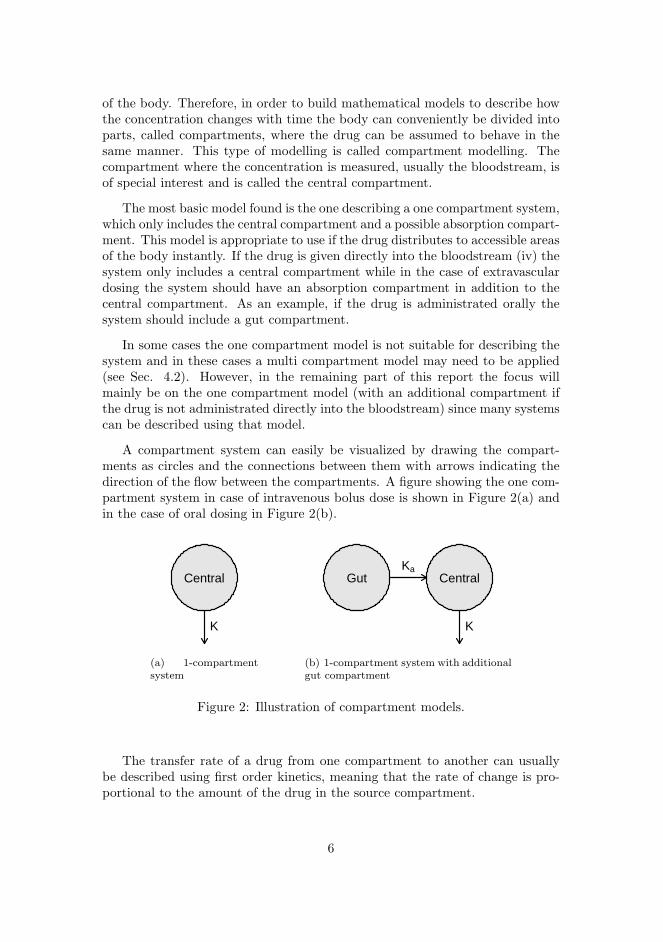
of the body. Therefore, in order to build mathematical models to describe howthe concentration changes with time the body can conveniently be divided intoparts, called compartments, where the drug can be assumed to behave in thesame manner. This type of modelling is called compartment modelling. Thecompartment where the concentration is measured, usually the bloodstream, isof special interest and is called the central compartment.
The most basic model found is the one describing a one compartment system,which only includes the central compartment and a possible absorption compart-ment. This model is appropriate to use if the drug distributes to accessible areasof the body instantly. If the drug is given directly into the bloodstream (iv) thesystem only includes a central compartment while in the case of extravasculardosing the system should have an absorption compartment in addition to thecentral compartment. As an example, if the drug is administrated orally thesystem should include a gut compartment.
In some cases the one compartment model is not suitable for describing thesystem and in these cases a multi compartment model may need to be applied(see Sec. 4.2). However, in the remaining part of this report the focus willmainly be on the one compartment model (with an additional compartment ifthe drug is not administrated directly into the bloodstream) since many systemscan be described using that model.
A compartment system can easily be visualized by drawing the compart-ments as circles and the connections between them with arrows indicating thedirection of the flow between the compartments. A figure showing the one com-partment system in case of intravenous bolus dose is shown in Figure 2(a) andin the case of oral dosing in Figure 2(b).
Central
K
(a) 1-compartmentsystem
Gut CentralKa
K
(b) 1-compartment system with additionalgut compartment
Figure 2: Illustration of compartment models.
The transfer rate of a drug from one compartment to another can usuallybe described using first order kinetics, meaning that the rate of change is pro-portional to the amount of the drug in the source compartment.
6
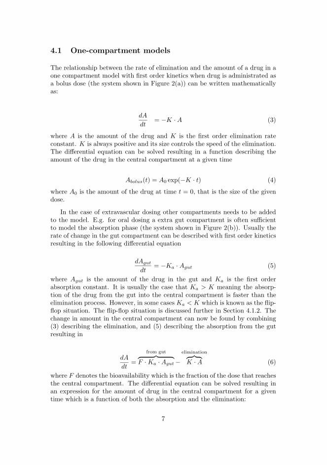
4.1 One-compartment models
The relationship between the rate of elimination and the amount of a drug in aone compartment model with first order kinetics when drug is administrated asa bolus dose (the system shown in Figure 2(a)) can be written mathematicallyas:
dA
dt= −K ·A (3)
where A is the amount of the drug and K is the first order elimination rateconstant. K is always positive and its size controls the speed of the elimination.The differential equation can be solved resulting in a function describing theamount of the drug in the central compartment at a given time
Abolus(t) = A0 exp(−K · t) (4)
where A0 is the amount of the drug at time t = 0, that is the size of the givendose.
In the case of extravascular dosing other compartments needs to be addedto the model. E.g. for oral dosing a extra gut compartment is often sufficientto model the absorption phase (the system shown in Figure 2(b)). Usually therate of change in the gut compartment can be described with first order kineticsresulting in the following differential equation
dAgut
dt= −Ka ·Agut (5)
where Agut is the amount of the drug in the gut and Ka is the first orderabsorption constant. It is usually the case that Ka > K meaning the absorp-tion of the drug from the gut into the central compartment is faster than theelimination process. However, in some cases Ka < K which is known as the flip-flop situation. The flip-flop situation is discussed further in Section 4.1.2. Thechange in amount in the central compartment can now be found by combining(3) describing the elimination, and (5) describing the absorption from the gutresulting in
dA
dt=
from gut︷ ︸︸ ︷F ·Ka ·Agut−
elimination︷ ︸︸ ︷K ·A (6)
where F denotes the bioavailability which is the fraction of the dose that reachesthe central compartment. The differential equation can be solved resulting inan expression for the amount of drug in the central compartment for a giventime which is a function of both the absorption and the elimination:
7

Aoral(t) =KaFA0
Ka −K(exp(−K · t)− exp(−Ka · t)) (7)
Equations (4) and (7) can now be used to describe the amount of drug inthe central compartment for a one compartment system in the case of a bolusdose and oral dosing, respectively. Usually it is more interesting to model theconcentration (C) in stead of the amount since it is the concentration of thedrug in the blood that is measured. According to (1) the concentration is foundby dividing the amount by the volume of distribution resulting in
Cbolus(t) =Abolus(t)
V=
A0
V· exp(−K · t) (8)
in the case of a bolus dose, and
Coral(t) =Aoral(t)
V=
KaFA0
V (Ka −K)(exp(−K · t)− exp(−Ka · t)) (9)
in the case of oral dosing.
4.1.1 Case study: pain reliever
To illustrate the use of compartment modelling the drug paracetamol will beused as a case study. Paracetamol is the active substrate in a large number ofpain relieving drugs on the market although its mechanism of action is still asource of debate. At correct dosages it works well against head ache and feverbut at very high dosages it can cause lasting damages on the liver. For adultsit is recommended to take doses of 1000mg at most 3-4 times a day and nevermore than 4g per day.
Paracetamol has been tested in a number of trails and it has been shownthat the pharmacokinetics can be adequately described by a multi-compartmentmodel structure, which will be introduced in Section 4.2 in further detail (see alsoRawlins et al. (1977)). As a good approximation however, it can be modelledusing a one-compartment model with a 1st order elimination from the bloodand likewise a 1st order absorption from the stomach. Paracetamol can thusbe modelled with the systems shown in Figure 2 for intravenous bolus and oraldosing. Based on Rawlins et al. (1977) the elimination rate constant can befound to K = 0.28h−1 and the volume of distribution is 0.60L/kg giving V =42L for an average 70kg adult. The absorption is controlled by an absorptionrate constant of Ka = 1.80h−1 and the bioavailability is found to F = 0.89.Note that Ka > K holds here, meaning that paracetamol is absorbed fasterthan it is eliminated.
Based on the information found for paracetamol it is possible to draw theconcentration as a function of time based on (8) and (9). This is called a
8

concentration profile and is shown for both intravenous bolus and oral dosingin Figure 3.
Hours
Kon
c. (
mg/
L)
0 3 6 90
10
20
(a) Intravenous (iv) bolus dose
Hours
Kon
c. (
mg/
L)
0 3 6 90
10
20tmax
Cmax
(b) Oral dose
Figure 3: Concentration profiles for dosing of 1000mg paracetamol.
Concentration profiles are also commonly shown with concentration on alog-scale as seen in Figure 4. This makes it possible to directly read off theelimination rate constant K as the slope of the line for intravenous bolus dos-ing. For oral dosing K is found as the slope of the last part of the profile(terminal slope) where it follows a straight line. This holds since Ka > K andthe absorption from the gut thus has finished so the drug is only contained inthe blood as for intravenous bolus dosing.
Hours
Kon
c. (
mg/
L)
∆t
∆(ln C)
0 3 6 9
2
5
20
50
(a) Intravenous (iv) bolus dose
Hours
Kon
c. (
mg/
L)
∆t
∆(ln C)
0 3 6 9
2
5
20
50
(b) Oral dose
Figure 4: Concentration profile on log-scale for dosing of 1000mg paracetamol.
In this case looking at Figure 4(b) we find approximately
K = −∆(log C)∆t
= − log 3− log 7.57h− 4h
≈ 0.305h−1 (10)
9

which compares well to the true value of K = 0.28h−1.
4.1.2 Flip-flop situation
Cases where the absorption rate constant is larger than the elimination rateconstant (Ka < K) is called a flip-flop situation. In these situations the absorp-tion will be the so-called rate limiting step in the final phase of the eliminationfor oral dosing (Gabrielsson and Weiner 1997) and thus the terminal slope fororal dosing will be −Ka instead of −K as shown in Figure 4(b). For intravenousdosing the slope is −K independent of Ka.
In order to be able to decide if it is a flip-flop situation it is necessary toperform both an intravenous bolus dosing study and an oral dosing study. Ifthe terminal slope of the oral dosing concentration profile is parallel to theintravenous bolus concentration profile it is a normal situation, since the finalelimination rates are equal. This can be known since the intravenous bolusconcentration profile consists only of an elimination phase without an absorptionphase.
On the other hand, if it is observed that the terminal slope for oral dosingis less steep than the intravenous bolus profile slope then the final phase mustbe absorption. The two situations are illustrated in Figure 5.
Time
log(
Con
c.) iv
oral
(a) Terminal phase for oral dosing is elimi-nation
Time
log(
Con
c.) iv
oral
(b) Terminal phase for oral dosing is absorp-tion
Figure 5: Situations with both elimination (normal) and absorption (flip-flop)as terminal phase seen as parallel and non-parallel terminal slopes respectively.
It is possible to determine the remaining rate constant (either Ka in a normalsituation and K in a flip-flop situation) using the method of residuals. This isexplained in detail in Gabrielsson and Weiner (1997).
10
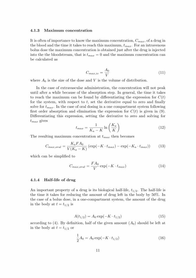
4.1.3 Maximum concentration
It is often of importance to know the maximum concentration, Cmax, of a drug inthe blood and the time it takes to reach this maximum, tmax. For an intravenousbolus dose the maximum concentration is obtained just after the drug is injectedinto the the bloodstream, that is tmax = 0 and the maximum concentration canbe calculated as
Cmax,iv =A0
V(11)
where A0 is the size of the dose and V is the volume of distribution.
In the case of extravascular administration, the concentration will not peakuntil after a while because of the absorption step. In general, the time it takesto reach the maximum can be found by differentiating the expression for C(t)for the system, with respect to t, set the derivative equal to zero and finallysolve for tmax. In the case of oral dosing in a one compartment system followingfirst order absorption and elimination the expression for C(t) is given in (9).Differentiating this expression, setting the derivative to zero and solving fortmax gives
tmax =1
Ka −Kln(
Ka
K
)(12)
The resulting maximum concentration at tmax then becomes
Cmax,oral =KaFA0
V (Ka −K)(exp(−K · tmax)− exp(−Ka · tmax)) (13)
which can be simplified to
Cmax,oral =FA0
Vexp(−K · tmax) (14)
4.1.4 Half-life of drug
An important property of a drug is its biological half-life, t1/2. The half-life isthe time it takes for reducing the amount of drug left in the body by 50%. Inthe case of a bolus dose, in a one-compartment system, the amount of the drugin the body at t = t1/2 is
A(t1/2) = A0 exp(−K · t1/2) (15)
according to (4). By definition, half of the given amount (A0) should be left atin the body at t = t1/2 or
12A0 = A0 exp(−K · t1/2) (16)
11

which can be simplified to
t1/2 =ln 2K
(17)
4.1.5 Constant rate infusion and multiple dosing
It is often the case that it is not enough for a patient to have effect of a drugduring the time span where a single pill or intravenous bolus dose is active inthe body. In some cases the solution is simply to give a higher dose, but sincethis may cause unwanted side effects, this is not always the best way to go.
Another possibility to prolong the effect of a drug is to give it as a constantrate infusion into the vein. This is the best way to control the drug flow intothe body and it is easily modelled for a constant rate Rin by
dC
dt=
Rin
V− CL
V· C (18)
assuming a one-compartment model with first order elimination. The solutionis given as
C(t) =Rin
CL
[1− exp
(−CL
Vt
)]. (19)
In some cases it is more practical to approximate the constant rate infusionby taking pills with a constant time interval. This is known as multiple dosingand is related to a constant rate infusion by the equation
Rin =F ·A0
τ(20)
where A0 is the dose in each pill, F is the bioavailability (the fraction thatreaches the blood) and τ is the time interval between dosing. The concentrationprofile for multiple dosing is a sum of single oral dosing profiles which can bewritten as
CMD(t) =N−1∑n=0
Coral(t− nτ) (21)
where N is the number of doses and Coral is given in (9).
The system is in steady state when the elimination rate equals the infusionrate, that is when
12

Rin
V=
CL
VCSS (22)
which gives a steady state concentration
CSS =Rin
CL. (23)
It can be shown by using (19) that 90% of CSS is reached after 3.32 half-lives. This result is independent of the rate of infusion which gives rise to thegeneral rule of thumb that 90% of steady state concentration is reached after3-4 half-lives (Gabrielsson and Weiner 1997).
Two examples of constant rate infusion and multiple dosing concentrationprofiles for paracetamol are shown in Figure 6.
Hours
Kon
c. (
mg/
L)
0 6 12 18 240
10
20
(a) 4 hours between oral dosing
Hours
Kon
c. (
mg/
L)
0 6 12 18 240
10
20
(b) 6 hours between oral dosing
Figure 6: Multiple dosing of 4g paracetamol with 4 oral doses of 1g shown as athick line. The dotted line is a constant rate infusion at a corresponding rate.
4.2 Multi-compartment models
It may be the case that the one-compartment model is not sufficient to describethe distribution and elimination of a drug. More complicated models whereadditional compartments are added to the central compartment, resulting ina multi-compartment system, should then be applied. As a consequence, thesystem consists of a central compartment, representing the bloodstream andrapidly equilibrated organs, one or more peripheral compartments, represent-ing more slowly equilibrating tissues, and finally in the case of extravascularadministration, an absorption compartment.
13

The expression for C(t) for a one compartment system (intravenous dosing)only includes a singe exponential term (Equation (4)). The best way to revealhow many compartments are needed to best describe the time course of theconcentration is to plot the concentration on a semi-logarithmic scale. Fora multi-compartment system this will most likely look like a piecewise linearfunction. As a general rule of thumb one compartment is needed for each linearpart that is identified. As an example a two compartment system in the case ofa bolus dose and the corresponding concentration profile are shown in Figure7. It can be seen by looking at the figure that the concentration profile consistsof two linear phases, a rapid initial and a slow terminal phase, which is the”fingerprint” of two-compartment systems.
Central
C1
Peripheral
C2
K12
K21
K
(a) Two-compartment system
Timelo
g(C
onc.
)
(b) Concentration profile for a two-compartment system
Figure 7: Illustration of two-compartment models.
The system shown in Figure 7(a) can be described mathematically usingtwo differential equations, where C1 and C2 represents the concentration in thecentral compartment and the peripheral compartment respectively.
dC1
dt= K21 · C2 −K12 · C1 −K · C1 (24)
dC2
dt= K12 · C1 −K21 · C2 (25)
A solution of the differential equations, that is an expression for the concentra-tion in the central compartment, can be written as
C = A · exp(−αt) + B · exp(−βt) (26)
Expressions for A,B, α, β given by K12, K21 and K can be found in Gabrielssonand Weiner (1997). The half-lives of the two phases can finally be calculated as
t1/2,α =log(2)
α(27)
and
t1/2,β =log(2)
β. (28)
14

4.2.1 Case study: pain reliever continued
To illustrate the use of compartment modelling, the intake of paracetamol wasmodelled using a one compartment model in Section 4.1.1. It has however beenshown that paracetamol concentration, after intravenous bolus dosis, follows abi-exponential decline indicating that a two compartment model should be usedto describe the system. Based on Rawlins et al. (1977), the time course of theconcentration following an intravenous bolus dose of 1000mg is given by
C(t) = 13.8 · exp(−2.55t) + 13.0 · exp(−0.28t) (29)
The resulting concentration profile is shown in Figure 8.
Hours
Kon
c. (
mg/
L)
0 3 6 9
2
5
20
50
Figure 8: Concentration profile for paracetamol (1000mg intravenous bolus).
5 PD modelling
This section contains a brief introduction to pharmacodynamics (PD). In phar-macodynamics the dependent variable is not always straight forward to define.The dependent variable in pharmacokinetics is amounts or concentrations ofthe drug but for pharmacodynamics the dependent variable is not so obvious.How is the effect of a drug measured? Drugs against high blood pressure orfewer can be measured on the actual drop in pressure or temperature. Withinepilepsy the desired effect of a drug should lower the number of seizures makingthe PD measurement a count. Within pain relieve the measurement can be ascale where the subject grades the pain and here the response variable will bean ordinal variable.
This wide variety of possible outcomes of a pharmacodynamic trial makes ithard to present a single methodology to handle all cases of PD modelling. This
15

section will focus on the most simple models and only with continuous responsevariables.
5.1 Receptor Theory
This section includes a quick introduction into receptor theory and how it helpsin the understanding of the pharmacodynamic response. The presentation ofthe receptor theory is highly inspired by Gabrielsson and Weiner (1997).
Before a drug molecule can give rise to a pharmacodynamic effect it needsto interact with the cells. The cell membrane is covered in different receptorseach with a specific structure. The structure defines which molecules that canattach to the receptor. In engineering terms a receptor can best be describedas a docking station. The drug binding to the receptor initiates a change in thestructure of the receptor and thereby changing the cell membrane.
Drugs are divided into two classes according to their function on the receptor.Agonists initiates a structural change in the receptor thereby changing the cellresulting in a response. Antagonists have a different role by simply binding tothe receptor but not inducing any response. By occupying the receptor it blocksthe receptor for other molecules. This is also why antagonists are sometimesreferred to as blockers.
The set of unoccupied receptors [R] placed on the target cells that potentiallycan bind with drug molecules [D] and their relation to the bound drug/receptorcomplex [DR] can be stated as
[D] + [R]k1
k−1
[DR] (30)
where D denotes the drug, R the receptors and DR the bound drug/receptorcomplex.
The equation is based on a reversible receptor that can release the drug andbe occupied by a new drug molecule. The constant k1 indicates the rate ofchange from unbound to bounded and k−1 the other way. The binding propertybetween the drug and the receptor determines the proportion of bound drug atequilibrium. The term affinity, which is often used to describe how good a drugbinds to the receptor, is defined as
Affinity =k1
k−1=
1Kd
. (31)
The inverse of the affinity is denoted the disassociation constant Kd as shownabove and is also often used.
16

The properties of association and disassociation determines the proportionsin each state at equilibrium. It is clear that both the willingness to associa-tion/bind and the ability to stay associated/connected affects the proportionsin equilibrium. One easy way to affect the amount of bound drug is simply toadd more drug.
The link from the drug/receptor complex to the pharmacodynamic responsecan be thought of as a direct link between the receptor occupancy and the re-sponse. However often an extra state is included although hard to measure. Theextra state extends the occupied state by introducing an occupied and activatedstate. It splits the assumption that an occupied receptor is automatically active.
Inactive︷ ︸︸ ︷[D] + [R] [DR]
Active complex︷ ︸︸ ︷[DR∗] (32)
Equation (32) should be interpreted using the concepts of binding and acti-vation. Now a drug can be specified as both having a property for binding andactivation of the receptor. This ability to activate the receptor is denoted in-trinsic activity and is more difficult to measure (Gabrielsson and Weiner 1997).
5.1.1 Michaelis-Menten model
It is possible to derive a model for the relation between drug concentration andeffect based on receptor theory. The effect response E is assumed proportionalto the occupancy of the receptors and thus that the maximal effect is achievedif all receptors [Rtot] are occupied. This can be stated as
E = α[RD] (33)Emax = α[Rtot] (34)
where [Rtot] = [R] + [RD] is the total number of receptors and Emax is themaximal effect and α is the proportionality constant.
The steady state conditions can be stated as
d[RD]dt
= k1[R][D]− k−1[RD] = 0
[R][D][RD]
=k−1
k1= Kd (35)
17

By substituting [R] with ([Rtot]− [RD])
[D]([Rtot]− [RD])[RD]
= Kd
[RD][Rtot]
=[D]
[D] + Kd(36)
Now by inserting the response assumptions
E/α
Emax/α=
[D][D] + Kd
E
Emax=
[D][D] + Kd
E =Emax[D][D] + Kd
(37)
The relationship in (37) is called a Michaelis-Menten relationship betweendrug concentration and the effect. This derivation demonstrates the motivationfor the use of saturable models in pharmacodynamic modelling. Physiologicallyit also makes sense that at some point increasing the drug concentration willnot result in a increased response.
The disassociation constant Kd determines the concentration at 1/2·Emax ascan be seen from (37). An example of the model on both normal and logarithmicscale is shown in Figure 9.
Emax
Kd
50%
0
(a) Response vs. Conc.
Emax
Kd
50%
0
(b) Response vs. log(Conc).
Figure 9: Michaelis-Menten relationship with response.
5.1.2 Commonly used PD models
The Michaelis-Menten relationship forms the basis of one of the most commonlyused models to describe the relation between effect and concentration. Thismodel is called the Sigmoid Emax model and is described by
18

E = E0 +EmaxCn
Cn + ECn50
(38)
where C is the concentration and EC50 is the concentration at E0 + 1/2 ·Emax.The extra parameter n is included to provide a more flexible model. The modelis often used with n = 1 and then simply called an Emax model.
In order to be able to estimate parameters in the (Sigmoid) Emax modelit necessary to have estimates of the effect all the way from E0 up to a pointwhere maximum effect E0 +Emax seems to have been reached. If this is not thecase it is often advisable to use a more simple model such a the linear model
E = E0 + S · C (39)
or the log-linear model
E = m · log(C + C0) . (40)
Both of the models will in many situations be able to adequately describethe observed concentration-effect relationship. A comparison of all three modelsare shown in Figure 10. For the Emax model n = 1, E0 = 3, Emax = 8 andEC50 = 100 and remaining parameters S, m and C0 are chosen so they all havethe same effect at concentrations of 0 and EC50.
0
E0
E0 + Emax
1 10 100 1000 10000
linearlog−linearEmax
Figure 10: Comparison of standard models in PD analysis.
5.2 Modelling with effect compartments
In many situations it is not enough to directly model the response as a functionof systemic concentrations in the PK model. This can happen if maximum effectis delayed compared to the maximum concentration.
19

This can numerically be handled by adding an additional compartment withconcentration Ce representing the near cell tissue. This is called an effect com-partment and is assumed to have a negligible volume. There will thus not beany mass transfer from the PK model. Furthermore a rate parameter govern-ing the time delay from systemic concentration C1 to near cell concentration isneeded and for identifiability the same parameter is often used as eliminationfrom the effect compartment. The model for the effect compartment is
dCe/dt = ke1C1 − ke0Ce . (41)
The response from the drug is now modelled as a link from the effect com-partment to the response. The link can be either a linear, log-linear, Michaelis-Menten or an even more complex relationship.
The response functions is often extended with the use of subject specificcovariates as this can increase the accuracy of the model.
5.2.1 Case study: pain reliever continued
This example shows how a PD model can be build on top of a PK model tomodel the effect after an oral dose of 1000mg paracetamol. The PK-model usedis the two-compartment model shown in Sec. 4.2.1. This is used in combinationwith a first order absorption from the gut. The PK model is defined belown in(42) to (44).
dCgut/dt = −KaCgut (42)dC1/dt = −k12C1 + k21C2 − k10C1 + FKaCgut (43)dC2/dt = k12C1 − k21C2 (44)
The PD model used in this example is taken from (Gibb and Anderson2008). It uses an effect compartment with an Emax model to model the effect.The effect compartment model is shown in (41) and is only a hypotheticalcompartment to introduce a delay of effect. It does thus not influence the PKmodel.
The compartment structure of the combined PK/PD model is shown inFigure 11. The arrows for the effect compartment are shown with dashed linesto indicate the there is no actual mass transfer.
The effect is measured on a visual analogue scale (VAS) from 0-10 wherereduction below 10 indicates pain relief. The Emax model for the effect is
20
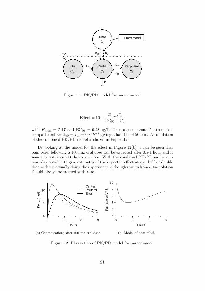
Effect
Ce
Gut
Cgut
Central
C1
Peripheral
C2
K12
K21
K
Ka
Ke1Ke0PD
PK
Emax model
Figure 11: PK/PD model for paracetamol.
Effect = 10− EmaxCe
EC50 + Ce
with Emax = 5.17 and EC50 = 9.98mg/L. The rate constants for the effectcompartment are ke0 = ke1 = 0.83h−1 giving a half-life of 50 min. A simulationof the combined PK/PD model is shown in Figure 12.
By looking at the model for the effect in Figure 12(b) it can be seen thatpain relief following a 1000mg oral dose can be expected after 0.5-1 hour and itseems to last around 6 hours or more. With the combined PK/PD model it isnow also possible to give estimates of the expected effect at e.g. half or doubledose without actually doing the experiment, although results from extrapolationshould always be treated with care.
Hours
Kon
c. (
mg/
L)
0 3 6 90
5
10CentralPeriferalEffect
(a) Concentrations after 1000mg oral dose.
Hours
Pai
n sc
ore
(VA
S)
0 3 6 95
6
7
8
9
10
(b) Model of pain relief.
Figure 12: Illustration of PK/PD model for paracetamol.
21

6 Modelling data
To work with real life data a model of a system must be able to handle noisyobservations. The models discussed until now has only been concerned withrelatively simple deterministic relationships, but real systems naturally containmuch more variation than suggested by these simple models. The remainingpart of the text will focus on how to extend these models to include a model forthe different types of variation found in data. The aim is to enable the use ofa reliable statistical framework for consistent inference, simulation, predictionand control by providing a proper description of the variation into the model.
The variation found in data can be caused by a number of sources. The mainsources include ordinary measurement variation and variation due to differencebetween individuals, sites, occasions, etc. There may also be stochastic fluctua-tions of the system within an individual or approximations in the applied model,which will also lead to variation in data that must be accounted for. Furthermore, the model for an individual may depend on an input process (e.g. roomtemperature) which is sampled continuously together with the response. Mea-surements of this process is normally assumed to be done without measurementerror, but if this is not true it will also lead to variation in the data that mustbe included in the model.
This section will discuss how to handle all of these different sources of vari-ation.
6.1 Single individual
The structure of data for a single individual is
yj , j = 1...n (45)
where yj is a possibly multi-dimensional response. The sub-index is short handnotation referring to the sampling times t0 < tj < tn.
6.1.1 Error model using ODEs
Modelling of PK for single individuals has traditionally been based on ordinarydifferential equations (ODEs) as for example done in a classical tool like NON-MEM (Beal and Sheiner 2004). The observed deviations from the deterministicpart of this model is treated as measurement error, which implies that the in-dividual is assumed to follow the model exactly, or stated differently that themodel represents the true state of the individual. This class of models can bestated as a state space model, which is written as
22

dxt = f(xt,ut, t,φ)dt (46)yj = h(xj ,uj , tj ,φ) + ej (47)
where xt is the state (vector) in the model and the model for the state is givenby (46). The parameters in the model are denoted φ, and ut is a vector of inputvariables to the system. The second equation (47) in the state space model isthe measurement equation defining how the states are observed. In this case anadditive error model is chosen, but this is only one of several choices. Both themeasurement and state equation can be multi-dimensional.
The states can represent amounts, concentrations, time-varying parametersor other dynamic parts of a system described by a state space model. At anypoint in time the state vector contains all the information about the futurewhich is known as the Markovian property. The input variables ut is a processinfluencing the system and it is observed only at measurement time points andis often assumed constant in between (known as zero order hold). A typicalinput variable could be e.g. body temperature or room temperature that mayaffect the system. The input process is assumed to be known exactly and as aconsequence future values of the states in a deterministic model can be predictedwithout uncertainty by solving the ODE.
In the following a one-compartment ODE model for an intravenous bolusdose will be used as an example. The model is described by
dxt = −kxt dt (48)
which is also shown in (3). Here xt represents concentration in the centralcompartment and k is the elimination rate constant.
Traditionally there are four main types of error models for the measurementequation called additive, multiplicative, additive and multiplicative, and log-normal error. The four error models are shown in (49), (50), (51) and (52)respectively, where ej , ej,1 and ej,2 are Normal IID random variables. In Figure13 the error models are illustrated graphically.
yj = xj + ej (49)yj = xj · (1 + ej) (50)yj = xj · (1 + ej,1) + ej,2 (51)yj = xj · exp(ej) (52)
The optimal choice of measurement error model is very dependent on thedata. The additive error model (49) is the simplest but may not always be
23
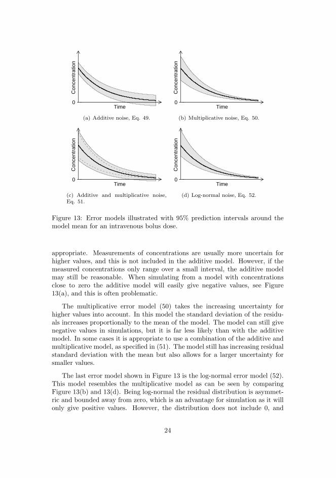
Time0
Con
cent
ratio
n
(a) Additive noise, Eq. 49.
Time0
Con
cent
ratio
n
(b) Multiplicative noise, Eq. 50.
Time0
Con
cent
ratio
n
(c) Additive and multiplicative noise,Eq. 51.
Time0
Con
cent
ratio
n
(d) Log-normal noise, Eq. 52.
Figure 13: Error models illustrated with 95% prediction intervals around themodel mean for an intravenous bolus dose.
appropriate. Measurements of concentrations are usually more uncertain forhigher values, and this is not included in the additive model. However, if themeasured concentrations only range over a small interval, the additive modelmay still be reasonable. When simulating from a model with concentrationsclose to zero the additive model will easily give negative values, see Figure13(a), and this is often problematic.
The multiplicative error model (50) takes the increasing uncertainty forhigher values into account. In this model the standard deviation of the residu-als increases proportionally to the mean of the model. The model can still givenegative values in simulations, but it is far less likely than with the additivemodel. In some cases it is appropriate to use a combination of the additive andmultiplicative model, as specified in (51). The model still has increasing residualstandard deviation with the mean but also allows for a larger uncertainty forsmaller values.
The last error model shown in Figure 13 is the log-normal error model (52).This model resembles the multiplicative model as can be seen by comparingFigure 13(b) and 13(d). Being log-normal the residual distribution is asymmet-ric and bounded away from zero, which is an advantage for simulation as it willonly give positive values. However, the distribution does not include 0, and
24

this is a problem if the observed data has such measurements. The log-normalerror model can be achieved with an additive error structure by using a log-transformation of the observations, i.e. log yj = µ∗ + ej where µ∗ = log µ. Aneffect of this is that if the model for µ∗ is additive then the resulting model forµ will be multiplicative since µ = exp(µ∗).
6.1.2 Error model using SDEs
In most cases it is not reasonable to assume that the variation in time of theconcentration for an individual follows the model exactly as it is assumed usingan ODE model. As mentioned earlier there may also be some variation due toincorrect model specification, true random biological variation or uncertaintyfrom measuring an input process which cannot be explained or included inthe ODE model. A way to describe such sources of errors is to base the statespace model on stochastic differential equations (SDEs) instead of ODEs. Thisis called a stochastic state space model and is defined as
dxt = f(xt,ut, t,φi)dt + σω(ut, t,φi)dωt (53)yj = h(xj ,uj , tj ,φi) + ej . (54)
The stochastic differential equation in (53) is based on the Standard Wienerprocess ωt (Øksendal 1992). This process is characterized by ω0 = 0, it is almostsurely continuous and it has independent normal increments with ωt − ωs ∼N(0, t− s) for 0 ≤ s < t. The Wiener process can be seen as a process that hasthe properties expected from the limit of a discrete random walk
∑t/∆ti=1 ei with
ei ∼ N(0,∆t) for ∆t → 0.
Using the Wiener process the simple one-compartment elimination model in(48) can be extended to a model based on SDEs by writing
dxt = −kxt dt + σωdωt . (55)
The term dωt is an infinitesimal increment of the Wiener process and themodel can thus in simple terms be described as an ordinary differential equationwhere the evolution in time is perturbed by normal distributed noise. Thesolution to (55) is
xt = x0e−kt +
∫ t
0
σωe−k(t−s)dωs (56)
25

which can be seen to be the ODE solution plus the integral of Wiener processincrements with exponential weights. The process is known as an Ornstein-Uhlenbeck process with zero mean. A simulation of the process is shown inFigure 14.
C
once
ntra
tion
0
20
40
60
80
100
0 20 40 60 80Time
Figure 14: Simulation of simple one-compartment SDE model (55).
There are a few problems with the model proposed in (55). There is nothinglimiting the concentration from increasing when the increments of the Wienerprocess are positive. This should normally not happen in the real world as thiswould require a reverse elimination process. Moreover the model will fluctuatearound zero when the initial dose has been eliminated, and the model will thuspredict negative concentrations. In fact it can be shown that the unconditionaldistribution of xt is normal with mean zero which is not suitable in a model forconcentrations.
A more realistic model can be achieved by adding noise to the eliminationrate constant k instead of directly to the concentration. A good first choice is tomodel kt as an Ornstein-Uhlenbeck process with a non-zero mean k. However,the elimination rate should never be negative, so the elimination rate used willbe k2
t . The model is given by
dxt = −k2t xt dt (57)
dkt = −γ(kt − k)dt +√
2σ2ωγdωt . (58)
It can be shown that the unconditional distribution of kt is normal with meanE[kt] = k and that kt has the autocorrelation function Ckt(t) = σ2
ω exp(−γt).Thus the elimination rate (k2
t ) will be χ2-distributed with mean E[k2t ] = k2+σ2
ω.In Figure 15 a simulation of the model is shown. Since the elimination rate inFigure 15(b) is always non-negative, the concentration curve will be monotonelydecreasing towards zero as would be expected in real life.
26

Time
Con
cent
ratio
n
0 20 40 60 800
20
40
60
80
100
(a) Concentration as state 1.
Time
kt2
20 40 60 800.0
0.1
(b) Elimination rate as state 2 squared.
Figure 15: Simulation of an extended one-compartment SDE model that fulfillssome basic physiological constraints.
6.1.3 Case study: Advantages of using SDEs
In order to illustrate the advantages of modelling using SDEs a small simulationstudy will be performed.
It is assumed that the drug of interest is eliminated based on the modelin (57) and (58). That is, the concentration is assumed to follow a first orderelimination with an elimination rate that varies in a non-deterministic way. Theoptimal model is thus naturally the SDE model that generates the data, sincethe non-deterministic variations of the elimination rate cannot be modelled anyfurther. However, the example will focus on illustrating the errors that areintroduced if the data is modelled using the simple ODE model shown in (48).The residual error will be assumed to be independently log-normally distributedas defined in (52). Combining this the state space model used for generatingdata contains two states and one response variable and is thus given by
dxt = −k2t xt dt (59)
dkt = −γ(kt − k)dt +√
2σ2ωγdωt (60)
log yj = log xj + ej (61)
which will in short be denoted the SDE model. The parameters used for thesimulation are k = 0.05, γ = 0.40 and σω = 0.15, which gives an expectedelimination rate of E[k2
t ] = 0.025 min−1 and an expected half-life of 28 minutes.The measurement variation is ej ∼ N(0, S) where S = 0.202. Dose is 100mgand volume of distribution is 10L giving an initial concentration of 100mg/L.The individual is sampled with 5 minute intervals up to 100 minutes giving 21observations. The simulated data is shown in Figure 16(a).
The data is modeled both using the original SDE model and an ODE modelwhere the stochastic part is removed. The ODE model is thus a standard one-
27

compartment model with first order elimination. The ODE model is definedas
dxt = −kxt dt (62)log yj = log xj + ej (63)
which is equivalent to the SDE model with σω = 0. Both the ODE model andSDE models are fitted using the maximum likelihood method, where the like-lihood function is evaluated using the Kalman Filter. The estimation methodis explained in more detail in Section 6.3. The estimate of the two states (con-centration and elimination rate) in the SDE model can be found based on theestimated parameters using the so-called Kalman smoothing estimate. The re-sults of the two model fits as given by the estimated concentration profiles areshown in Figure 16(b) and 16(c).
In order to judge the model fits the residuals for the ODE and SDE modelsare shown in Figure 16(d) and 16(e) and the auto-correlation functions for theresiduals are shown in Figure 16(f) and 16(g).
The first obvious observation of the difference between the fits is that thesimple ODE model cannot capture the time varying elimination rate which givesrise to persistence in time of the residuals. This is not the case for the SDEmodel, which assumes a stochastic elimination rate and estimates it based onthe model and data. The result is that the residuals are uncorrelated in timefor SDE model whereas they are strongly auto-correlated for the ODE model.This in effect falsifies the ODE model in this case, as both models are based onan assumption of uncorrelated measurement error.
The problem is also apparent from the parameter estimates them selves. Theestimates of the measurement variation in the two models are SODE = 0.392
and SSDE = 0.222 which should be compared to the true value of S = 0.202.This shows that the time variation of the elimination rate has been included inthe measurement error in the ODE model, since this is the only place it allowsvariation to enter, and hence a wrong interpretation of the measurement erroris provided by the ODE model.
It is of interest to see if the estimate in the SDE model of the time varyingbehavior of the elimination rate (k2
t ) is accurate. Figure 17 shows the outcomeof the elimination rate process from the simulation compared to the Kalmansmoothing estimate from the SDE model and also the constant estimate fromthe ODE model. Generally it appears that the Kalman smoothing estimate isfairly close to the true elimination rate, but the accuracy will naturally always bedependent on the kind of measurement noise, sampling rate and appropriatenessof the assumed model.
28

Time
Con
cent
ratio
n
0 20 40 60 80 1000
20
40
60
80
100
(a) Simulated data from model based on SDEs.
Time
log
Con
c.
0 20 40 60 80 1002
51020
50100 ODE model
(b) Fitted ODE model on log-scale.
Time
log
Con
c.
0 20 40 60 80 1002
51020
50100 SDE model
(c) Fitted SDE model on log-scale.
Time
resi
dual
s (lo
g)
0 20 40 60 80 100
−0.5
0.0
0.5
(d) Residuals in ODE model.
Time
resi
dual
s (lo
g)
0 20 40 60 80 100
−0.5
0.0
0.5
(e) Residuals in SDE model.
corr
elat
ion
0 1 2 3 4 5 6 7 8 9 10
−0.5
0.0
0.5
1.0
(f) ODE residual auto-correlation.
corr
elat
ion
0 1 2 3 4 5 6 7 8 9 10
−0.5
0.0
0.5
1.0
(g) SDE residual auto-correlation.
Figure 16: Comparison of fitted ODE and SDE models.
29

Time
kt2
0 20 40 60 800.0
0.1
0.2
SDE modelODE modelSimulation
Figure 17: Comparison of estimated elimination rates.
6.1.4 Discussion of SDEs
The previous example in Section 6.1.3 has illustrated some of the issues thatarise in a case where an ODE model provides an insufficient error structure.The estimate of the measurement variation was seen to be to high since it alsoincluded the stochastic variation of the system, and it resulted in auto-correlatedresiduals. Such situations calls for the use of an SDE model. In other situationsan SDE model may be justified by a need to capture variation in the statesintroduced by actual stochastic behavior or a too simple deterministic part of amodel or by variation caused by measurement error from the input process.
For estimation in the previous example both models were used in a maximumlikelihood frame work. From a likelihood perspective, the failure of the ODEmodel occurs since it is not able to give a sufficient description of the ’true’likelihood function. Such an error cannot be ignored, as it in turn will invalidatee.g. likelihood ratio tests for model reduction and other classical statistical teststhat may be used.
In many ways modeling using SDEs seems like an intuitive choice, since itfacilitates a way to include dynamic biological variation in the model. Oftenhowever, the need for an SDE model is hidden by a sparse sampling scheme withfew and distant observations, since it can be hard to detect residual autocorre-lation in these situations. This may however change in the future with increas-ing use of modern frequent-sampling equipment within many areas, which verylikely will reveal residual auto-correlation when using standard ODE models.
An example has been shown by Overgaard et al. (2007) using a PK/PDmodel of effects on thermo-regulation in monkeys. In this case an ODE modelis shown to be insufficient, and only a model based on SDEs is able to providea proper description of the error structure. Due to this the SDE model is ableto give realistic simulations and predictions as opposed to the ODE model.Generally, in cases where the model should also be used for control purposes itis important that the model has realistic prediction properties. An example ofan application for control of a biological system could be a model for controlling
30

the insulin secretion rate in diabetic patients.
Another application of SDEs in modelling biological systems is to use it asa tool for model development. In this context SDEs can be used as a tool toextract information from data about the appropriate model in situations with acomplex underlying deterministic model structure. In Kristensen et al. (2005)a framework is presented for using an SDE model to allow tracking of timevariations of parameters to reveal new functional relationships. Although thisuse aims at improving the deterministic part of a model, it may still resulta final model based on SDEs if all stochastic components cannot replaced bydeterministic relationships.
6.2 Multiple individuals
A typical data set for PK/PD modelling consists of data from several individualswho all have been exposed to a similar trial. The previous section has beenconcerned with modelling a single individual, but it is natural to include allindividuals in the same model.
A mixed-effects model allows this by assuming the same model for eachindividual and by further assuming that the parameters in this model can varybetween individuals. The general structure for data in a mixed-effects model is
yij , i = 1, ..., N, j = 1, ..., ni (64)
which is an extension of the data structure in (45). The response yij is a vectorof measurements at time tij for individual i, N is the number of individuals andni is the number of measurements for individual i.
In a mixed-effects model the variation is split into intra-individual variationand inter-individual variation, which is modelled by a first and second stagemodel. The first stage model is the (stochastic) state space model and thesecond stage model is given by
φi = g(θ,ηi,Zi) (65)
where φi are the individual parameters for the first stage model. The randomeffects ηi have the distribution ηi ∼ N(0,Ω), θ are the fixed effects (also calledpopulation parameters) and Zi are possible covariates. The second stage modelwill often look like φ = θ+η or φ = θ ·exp η giving either a normal or log-normaldistribution of parameters between individuals.
31

6.3 Estimation
Parameter estimation in the mixed effects model is most often facilitated by themaximum likelihood method. The population likelihood function is based onthe distribution functions for the first and second stage models denoted p1 andp2, respectively. The distribution function for the second stage model is simplythe normal distribution. For the first stage model based on the stochastic statespace model the likelihood function can be evaluated by using the Kalman filter(Overgaard et al. 2005). The population likelihood function for the fixed effectsare found by integration over the random effects. This is given as
L(θ) =N∏
i=1
∫p1(Yini
|θ,ηi)p2(ηi|Ω)dηi =N∏
i=1
∫exp(li)dηi (66)
where Yiniare all observations for individual i and li is the a posteriori log-
likelihood function for the ith individual. The population likelihood functionin (66) can not be evaluated analytically, and therefore li is approximated by asecond-order Taylor expansion, where the expansion is made around the valueη∗i that maximizes li(ηi) in the value l∗i . At this optimum the first derivative∇li
∣∣η∗i
= 0 and the population likelihood function therefore reduces to
L(θ) ≈N∏
i=1
∣∣∣∣−∆l∗i2π
∣∣∣∣− 12
exp(l∗i ) (67)
as shown in Appendix A. The approximation of the 2nd derivative at theoptimum ∆l∗i is obtained using the First-Order Conditional Estimation (FOCE)method, which is defined as
∆l∗i ≈ −ni∑
j=1
(∇εT
ijR−1i(j|j−1)∇εij
)−Ω−1 , ∇εij =
∂
∂ηi
εij
∣∣∣η∗i
.
In cases where the fist stage model is non-linear as in the state space modelin (53) and (54) the combined model is called a non-linear mixed effects model.When working with SDEs there are only a few software tools available that areable to estimate parameters in this class of models. These tools are listed below.
6.3.1 NONMEM
NONMEM is a software package developed at University of California, SanFrancisco (UCSF) for use in population PK/PD modelling (Beal and Sheiner
32

2004). It first appeared in 1979 and its name is an acronym for non-linearmixed effects modeling. NONMEM has become the defacto standard softwaretool used for PK/PD modelling as it is a very flexible tool and well testedthroughout many years of development. NONMEM is however only intendedfor modelling based on ODEs but it is possible to make it estimate models basedon SDEs as shown by Tornøe et al. (2005). This is basically done by includingthe Kalman filter into the model definition, but the Kalman filter has to bederived and implemented for every new model that is created, and it is thuscumbersome to work with and only feasible for simple models.
6.3.2 CTSM
CTSM is a program for performing estimation of state space models based onSDEs (Kristensen and Madsen 2003, Kristensen et al. 2004). The program isintended for single subject modelling but also handles multiple subjects basedon a pooled likelihood without random effects. It has been developed at DTUInformatics. CTSM has previously been used for PK/PD modelling using SDEsin e.g. Tornøe et al. (2004a, 2004b) and Kristensen et al. (2005).
6.3.3 PSM
PSM in an acronym for Population Stochastic Modelling and is a software pack-age developed at DTU Informatics (Mortensen et al. 2007, Klim et al. 2008). Itis like NONMEM aimed at non-linear mixed effects modelling but it is focusedon modelling using SDEs and as opposed to NONMEM it also directly handlesa multivariate response. PSM supports a typical PK data structure with dosinginformation, co-variates and also missing observations. PSM is freely availableas an extension package for R, which is a free software environment for statis-tical computing. Instructions for download and installation in R can found athttp://www.imm.dtu.dk/psm.
Appendix
A NLME log-likelihood function
The Non-linear mixed effects likelihood function is defined as
33

L(θ|YNni) =N∏
i=1
∫p1(Yini |θ,ηi)p2(ηi|Ω)dηi (68)
=N∏
i=1
∫Li(ηi)dηi (69)
where Li is the individual a posteriori likelihood function. In most cases theintegral cannot be evaluated analytically. For a general evaluation the individuala posteriori likelihood function can be approximated by a second order Taylorseries expansion of log(Li) around the value η∗i which maximizes log(Li(ηi)).Also li = log(Li), L∗i = exp(l∗i ) = Li(η∗i ), ∇l∗i = ∂
∂ηili
∣∣∣η∗i
, ∆l∗i = ∂2
∂ηi∂ηTi
li
∣∣∣η∗i
.
It follows that
li(ηi) ≈ l∗i + ∇l∗Ti (ηi − η∗i ) +12(ηi − η∗i )T ∆l∗i (ηi − η∗i ) (70)
≈ l∗i +12(ηi − η∗i )T ∆l∗i (ηi − η∗i ) (71)
Li(ηi) ≈ L∗i exp(−1
2(ηi − η∗i )T (−∆l∗i )(ηi − η∗i )
)(72)
since ∇li = 0 at η∗i . Based on the approximation the integral can now beevaluated by moving constants such that the integral is over a Gaussian densitywith mean η∗i and co-variance (−∆l∗i )−1 . The result is
∫Li(ηi)dηi ≈
∫L∗i exp
(−1
2(ηi − η∗i )T (−∆l∗i )(ηi − η∗i )
)dηi (73)
≈ L∗i
∣∣∣∣ 2π
−∆l∗i
∣∣∣∣ 12 ∫ ∣∣∣∣ 2π
−∆l∗i
∣∣∣∣− 12
exp(−1
2(ηi − η∗i )T (−∆l∗i )(ηi − η∗i )
)dηi
≈ L∗i
∣∣∣∣ 2π
−∆l∗i
∣∣∣∣ 12 (74)
≈ L∗i
∣∣∣∣−∆l∗i2π
∣∣∣∣− 12
(75)
where the step in Eq. (75) is taken to avoid a matrix inversion of the Hessian.The NLME log-likelihood function can now be approximated by
L(θ|YNni) ≈N∏
i=1
L∗i
∣∣∣∣−∆l∗i2π
∣∣∣∣− 12
. (76)
34

References
Beal, S. L. and L. B. Sheiner (2004). NONMEM R© Users Guide. NONMEMProject Group, University of California, San Francisco.
Gabrielsson, J. and D. Weiner (1997). Pharmacokinetic and PharmacodynamicData Analysis: Concepts and Applications (Second ed.). Kristianstads Bok-tryckeri.
Gibb, I. A. and B. J. Anderson (2008). Paracetamol (acetaminophen) pharma-codynamics: interpreting the plasma concentration. Arch. Dis. Child. 93 (3),pp. 241–247.
Klim, S., S. B. Mortensen, N. R. Kristensen, R. V. Overgaard, and H. Madsen(2008). Population stochastic modelling (PSM) - An R package for mixed-effects models based on stochastic differential equations. Technical report,DTU Informatics. Submitted to Comput. Methods Programs Biomed.
Kristensen, N. R. and H. Madsen (2003). Continuous time stochastic modelling- CTSM 2.3 Mathematics guide. Technical report, Technical University ofDenmark.
Kristensen, N. R., H. Madsen, and S. H. Ingwersen (2005). Using stochas-tic differential equations for pk/pd model development. J. Pharmacokinet.Pharmacodyn.. 32, pp. 109–41.
Kristensen, N. R., H. Madsen, and S. B. Jørgensen (2004). Parameter estimationin stochastic grey-box models. Automatica 40, pp. 225–237.
Mortensen, S. B., S. Klim, B. Dammann, N. R. Kristensen, H. Madsen, andR. V. Overgaard (2007). A matlab framework for estimation of nlme modelsusing stochastic differential equations: applications for estimation of insulinsecretion rates. J. Pharmacokinet. Pharmacodyn. 34 (5), pp. 623–642.
Overgaard, R. V., N. Holford, K. A. Rytved, and H. Madsen (2007). PKPDmodel of interleukin-21 effects on thermoregulation in monkeys–applicationand evaluation of stochastic differential equations. Pharm. Res. 24 (2), pp.298–309.
Overgaard, R. V., N. Jonsson, C. W. Tornøe, and H. Madsen. (2005). Non-linearmixed-effects models with stochastic differential equations: implementation ofan estimation algorithm. J. Pharmacokinet. Pharmacodyn. 32 (1), pp. 85–107.
Rawlins, M. D., D. B. Henderson, and A. R. Hijab (1977). Pharmacokineticsof paracetamol (acetaminophen) after intravenous and oral administration.Eur. J. Clin. Pharmacol. 11 (4), pp. 283–286.
Rowland, M. and T. N. Tozer (1997). Clinical Pharmacokinetics - Concepts andApplications (Third ed.). Lippincott Williams & Wilkins.
35
Tornøe, C. W., J. L. Jacobsen, and H. Madsen (2004a). Grey-box pharmacoki-netic/pharmacodynamic modelling of a euglycaemic clamp study. J. Math.Biol. 48 (6), pp. 591–604.
Tornøe, C. W., J. L. Jacobsen, O. Pedersen, T. Hansen, and H. Madsen (2004b).Grey-box modelling of pharmacokinetic/pharmacodynamic systems. J. Phar-macokinet. Pharmacodyn. 31 (5), pp. 401–417.
Tornøe, C. W., R. V. Overgaard, H. Agersø, H. A. Nielsen, H. Madsen, and E. N.Johnson (2005). Stochastic differential equations in NONMEM R©: Imple-mentation, application, and comparison with ordinary differential equations.Pharm. Res. 22 (8), pp. 1247–1258.
Øksendal, B. (1992). Stochastic differential equations (3rd ed.): an introductionwith applications. New York, NY, USA: Springer-Verlag New York, Inc.
36

120 Paper B
Appendix C
Paper C
Title:Population stochastic modelling (PSM) - An R package for mixed-effects modelsbased on stochastic differential equations.
Authors:S. Klim, S. B. Mortensen, N. R. Kristensen, R. V. Overgaard, and H. Madsen.
Published in:Computer Methods and Programs in Biomedicine 94, pp. 279-289 (2009).

c o m p u t e r m e t h o d s a n d p r o g r a m s i n b i o m e d i c i n e 9 4 ( 2 0 0 9 ) 279–289
journa l homepage: www. int l .e lsev ierhea l th .com/ journa ls /cmpb
Population stochastic modelling (PSM)—An R package formixed-effects models based on stochastic differentialequations
Søren Klima,c,∗, Stig Bousgaard Mortensenb,c, Niels Rode Kristensena,Rune Viig Overgaarda, Henrik Madsenc
a Novo Nordisk A/S, Novo Alle, 2880 Bagsværd, Denmarkb H. Lundbeck A/S, Ottiliavej 9, 2500 Valby, Denmarkc Department of Informatics and Mathematical Modelling, Technical University of Denmark,2800 Kgs. Lyngby, Denmark
a r t i c l e i n f o
Article history:
Received 26 August 2008
Received in revised form
30 January 2009
Accepted 1 February 2009
Keywords:
Stochastic differential equations
(SDEs)
State-space models
Mixed-effect
Pharmacokinetic
Pharmacodynamic
a b s t r a c t
The extension from ordinary to stochastic differential equations (SDEs) in pharmacokinetic
and pharmacodynamic (PK/PD) modelling is an emerging field and has been motivated in a
number of articles [N.R. Kristensen, H. Madsen, S.H. Ingwersen, Using stochastic differential
equations for PK/PD model development, J. Pharmacokinet. Pharmacodyn. 32 (February(1))
(2005) 109–141; C.W. Tornøe, R.V. Overgaard, H. Agersø, H.A. Nielsen, H. Madsen, E.N. Jonsson,
Stochastic differential equations in NONMEM: implementation, application, and compari-
son with ordinary differential equations, Pharm. Res. 22 (August(8)) (2005) 1247–1258; R.V.
Overgaard, N. Jonsson, C.W. Tornøe, H. Madsen, Non-linear mixed-effects models with
stochastic differential equations: implementation of an estimation algorithm, J. Pharma-
cokinet. Pharmacodyn. 32 (February(1)) (2005) 85–107; U. Picchini, S. Ditlevsen, A. De Gaetano,
Maximum likelihood estimation of a time-inhomogeneous stochastic differential model of
glucose dynamics, Math. Med. Biol. 25 (June(2)) (2008) 141–155].
PK/PD models are traditionally based ordinary differential equations (ODEs) with an obser-
vation link that incorporates noise. This state-space formulation only allows for observation
noise and not for system noise. Extending to SDEs allows for a Wiener noise component in
the system equations. This additional noise component enables handling of autocorrelated
residuals originating from natural variation or systematic model error. Autocorrelated resid-
uals are often partly ignored in PK/PD modelling although violating the hypothesis for many
standard statistical tests.
This article presents a package for the statistical program R that is able to handle SDEs in
a mixed-effects setting. The estimation method implemented is the FOCE1 approximation
to the population likelihood which is generated from the individual likelihoods that are
approximated using the Extended Kalman Filter’s one-step predictions.
© 2009 Elsevier Ireland Ltd. All rights reserved.
∗ Corresponding author at: DTU Informatics, Technical University of Denmark, Richard Petersens Plads, Building 321, 2800 Kgs. Lyngby,Denmark. Tel.: +45 4525 3351.
E-mail addresses: [email protected], [email protected] (S. Klim).1 FOCE—First-Order Conditional Estimation.
0169-2607/$ – see front matter © 2009 Elsevier Ireland Ltd. All rights reserved.doi:10.1016/j.cmpb.2009.02.001

280 c o m p u t e r m e t h o d s a n d p r o g r a m s i n b i o m e d i c i n e 9 4 ( 2 0 0 9 ) 279–289
1. Introduction
The use of mixed-effects models based on ordinary differ-ential equations (ODEs) is the standard for pharmacokineticand pharmacodynamic (PK/PD) modelling. The use of stochas-tic differential equations (SDEs) is an emerging field and hasbeen introduced and motivated in the papers [1–4]. This paperpresents an accessible software package for handling dynamicmodels based on SDEs in a mixed-effects setting. The programis a package for the statistical program R and thereby easy toinstall through R’s interface and available for a wide range ofoperating systems.
The package implements the (Extended) Kalman Filter forevaluating the likelihood function in models based on SDEs.The parameter estimation procedure in the package is maxi-mum likelihood based with fixed effects estimation based onthe FOCE approximation.
2. Computational methods and theory
The most widely used program to analyze state-space mod-els in PK/PD-modelling is NONMEM [5], which is focused onmixed-effects models based on ordinary differential equa-tions. The use of SDEs in non-linear mixed-effects modelsis possible in NONMEM as described in [2]. The trick is animplementation of the Extended Kalman Filter in the NON-MEM control file with corresponding adjustments to the datafile. This is a non-trivial task even for rather simple modelsand must be repeated for every change in model or data. Sin-gle subject data can be modelled with stochastic differentialequations in the program CTSM [6]. CTSM is a stand aloneprogram that works across different platforms.
The matlab framework described in [7] handles SDEs in amixed-effect setting. The experiences collected in the devel-opment of the Matlab framework have now been used to createan extended and more flexible R-package PSM.
The mathematical basis for the PSM package is alsodescribed in the articles [3,7,8]. It should be noted that thereare notation differences between the articles.
For simplicity this article focuses on the class of linear mod-els but it must be emphasised that the package also handlesnon-linear models.
2.1. Single subject
The modelling of observations for a single subject is based ona continuous-discrete state-space model. The states representthe internal hidden states of the system. The states reside in acontinuous time domain and their dynamics are described bystochastic differential equations. The observations are sam-pled at discrete time points and hence described by a discretetime relation.
The class of linear models handled by PSM are time-invariant models meaning that system matrices do not changeover time. More specifically the linear state-space model canbe stated as
dxt = (A(i)xt + B(i)ut) dt + (i)dωt (1)
yik = C(i)xik + D(i)uik + eik (2)
where xt ∈RdimX is the vector of states at time t. The dimen-sion of x is denoted as dimX for simplicity. A, B, C and D aretime-invariant matrices defined as functions of i with prop-erties A(·) ∈RdimX×dimX, B(·) ∈RdimX×dimU, C(·) ∈RdimY×dimX andD(·) ∈RdimY×dimU. i is the parameter vector for the ith indi-vidual (see Eq. (9) for further details). The exogenous inputu ∈RdimU can be used to include other measured variableswhich influence the time evolution of the states in the model.The input u is assumed to be constant between observationpoints which is often refered to as zero-order hold or piecewise constant. The component (i)dωt is the system noiseconsisting of a scaling diffusion term (·) ∈RdimX×dimX and ωt
which is a dimX-dimensional Wiener process. The subscripti denotes the ith subject and the subscript k is a short handnotation for tk. yik is the observation at time tk for the ith sub-ject. eik is the residual for individual i at time tk and is assumedto normal distributed N(0, S(i)) with S(·) ∈RdimY×dimY being thecovariance matrix for the errors.
2.2. Kalman Filter
The deterministic behaviour of ordinary differential equationscan be handled with standard differential equation solvers.The additional component in the SDE systems requires a moreadvanced solution method. As mentioned in the introductionthis package uses the Kalman Filter as solution method forsystems of SDEs.
The Kalman Filter is only briefly explained in this article butthe mathematics behind the Kalman Filter is well described inthe Mathematics guide to CTSM [6] and in the original refer-ence [9]. Several links and additional material can be found onthe homepage [10].
The assumptions on system noise being driven by a Wienerprocess and normally distributed errors will in a linear systemunder some regularity conditions [6] result in the conditionaldensities for the observations being fully described by theirfirst- and second-order moments. The Kalman Filter can beused to determine the optimal internal states in the systemconditioning on prior observations. The Kalman Filter updatesthe internal state vector after each observation and during thisprocess the Kalman Filter needs to weigh the probability ofthe residual being due to system noise or measurement noise.For this purpose the one-step prediction yk|k−1 and associatedcovariance Rk|k−1 are defined below:
yk|k−1 = E[yk|Yk−1, i] (3)
Rk|k−1 = V[yk|Yk−1, i] (4)
where Yk−1 denotes all measurements up to time tk−1.The description of conditional densities based on first- and
second-order moments is only exact for linear models. Fornonlinear models the Extended Kalman Filter can be usedwhich is based on continous linerazations of the model how-ever the forming of the conditional densitites will only beapproximate.
The structure of the Kalman Filter is thus an iterativeprocess with a prediction/updating scheme. The one-step
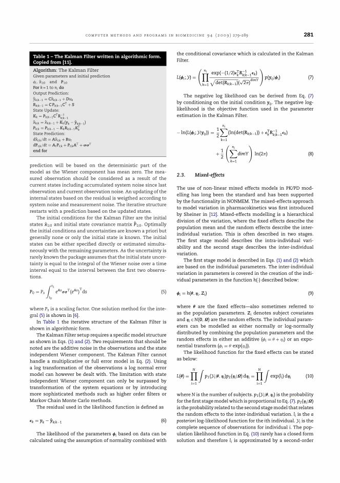
c o m p u t e r m e t h o d s a n d p r o g r a m s i n b i o m e d i c i n e 9 4 ( 2 0 0 9 ) 279–289 281
Table 1 – The Kalman Filter written in algorithmic form.Copied from [11].
Algorithm: The Kalman FilterGiven parameters and initial predictioni, x1|0 and P1|0For k = 1 to ni doOutput Prediction:yk|k−1 = Cxk|k−1 + Duk
Rk|k−1 = C Pk|k−1CT + S
State Update:Kk = Pk|k−1CTR−1
k|k−1
xk|k = xk|k−1 + Kk(yk − yk|k−1)Pk|k = Pk|k−1 − KkRk|k−1KT
k
State Prediction:dxt|k/dt = Axt|k + But
dPt|k/dt = AtPt|k + Pt|kAT + T
end for
prediction will be based on the deterministic part of themodel as the Wiener component has mean zero. The mea-sured observation should be considered as a result of thecurrent states including accumulated system noise since lastobservation and current observation noise. An updating of theinternal states based on the residual is weigthed according tosystem noise and measurement noise. The iterative structurerestarts with a prediction based on the updated states.
The initial conditions for the Kalman Filter are the initialstates x1|0 and initial state covariance matrix P1|0. Optimallythe initial conditions and uncertainties are known a priori butgenerally none or only the initial state is known. The initialstates can be either specified directly or estimated simulta-neously with the remaining parameters. As the uncertainty israrely known the package assumes that the initial state uncer-tainty is equal to the integral of the Wiener noise over a timeinterval equal to the interval between the first two observa-tions.
P0 = Ps
∫ t1
t0
eAsT(eAs)T
ds (5)
where Ps is a scaling factor. One solution method for the inte-gral (5) is shown in [6].
In Table 1 the iterative structure of the Kalman Filter isshown in algorithmic form.
The Kalman Filter setup requires a specific model structureas shown in Eqs. (1) and (2). Two requirements that should benoted are the additive noise in the observations and the stateindependent Wiener component. The Kalman Filter cannothandle a multiplicative or full error model in Eq. (2). Usinga log transformation of the observations a log normal errormodel can however be dealt with. The limitation with stateindependent Wiener component can only be surpassed bytransformation of the system equations or by introducingmore sophisticated methods such as higher order filters orMarkov Chain Monte Carlo methods.
The residual used in the likelihood function is defined as
k = yk − yk|k−1 (6)
The likelihood of the parameters i based on data can becalculated using the assumption of normality combined with
the conditional covariance which is calculated in the KalmanFilter.
L(i;Y) =(
ni∏k=1
exp(−(1/2)Tk
R−1k|k−1k)√
det(Rk|k−1)(√
2)dimY
)p(y0|i) (7)
The negative log likelihood can be derived from Eq. (7)by conditioning on the initial condition y0. The negative log-likelihood is the objective function used in the parameterestimation in the Kalman Filter.
− ln(L(i;Y|y0)) = 12
ni∑k=1
(ln(det(Rk|k−1)) + Tk R−1
k|k−1k)
+ 12
(ni∑
k=1
dimY
)ln(2) (8)
2.3. Mixed-effects
The use of non-linear mixed effects models in PK/PD mod-elling has long been the standard and has been supportedby the functionality in NONMEM. The mixed-effects approachto model variation in pharmacokinetics was first introducedby Sheiner in [12]. Mixed-effects modelling is a hierarchicaldivision of the variation, where the fixed effects describe thepopulation mean and the random effects describe the inter-individual variation. This is often described in two stages.The first stage model describes the intra-individual vari-ability and the second stage describes the inter-individualvariation.
The first stage model is described in Eqs. (1) and (2) whichare based on the individual parameters. The inter-individualvariation in parameters is covered in the creation of the indi-vidual parameters in the function h(·) described below:
i = h(, i, Zi) (9)
where are the fixed effects—also sometimes referred toas the population parameters. Zi denotes subject covariatesand i ∈ N(0, ˝) are the random effects. The individual param-eters can be modelled as either normally or log-normallydistributed by combining the population parameters and therandom effects in either an additive (i = + i) or an expo-nential transform (i = exp(i)).
The likelihood function for the fixed effects can be statedas below:
L() =N∏
i=1
∫p1(Yi|, i)p2(i|˝) di =
N∏i=1
∫exp(li) di (10)
where N is the number of subjects. p1(Yi|, i) is the probabilityfor the first stage model which is proportional to Eq. (7). p2(i|˝)is the probability related to the second stage model that relatesthe random effects to the inter-individual variation. li is the aposteriori log-likelihood function for the ith individual. Yi is thecomplete sequence of observations for individual i. The pop-ulation likelihood function in Eq. (10) rarely has a closed formsolution and therefore li is approximated by a second-order

282 c o m p u t e r m e t h o d s a n d p r o g r a m s i n b i o m e d i c i n e 9 4 ( 2 0 0 9 ) 279–289
Taylor expansion, where the expansion is made around thevalue i that maximizes li. At this optimum the first derivative∇li|i
= 0 and the population likelihood function will undersome assumptions reduce to
L() ≈N∏
i=1
∣∣∣−li2
∣∣∣−(1/2)
exp(li)| i(11)
The approximation of the 2nd derivative li is done usingthe First-Order Conditional Estimation (FOCE) method, whichis defined as
l∗i ≈ −ni∑
j=1
(∇Tij R
−1i(j|j−1)∇ij) − ˝−1, where ∇ij = ∂
∂iij|∗
i
(12)
When the random effects have a non-linear influence onthe likelihood through the first stage model, the combinedmodel is called a non-linear mixed effects model.
The conditional residual covariance R−1i(j|j−1) is calculated in
the (Extended) Kalman Filter and the gradient in the residualwith relation to the random effects ∇ij is typically found bynumerical methods.
2.4. Maximum likelihood estimation
The population likelihood function in (11) is used in max-imum likelihood estimation of the population parameters.This optimization becomes a nested optimization as the FOCEapproximation is based on the optimal random effects (∗
i).
Each calculation of the population likelihood thus requires Noptimizations of the random effects. This nested optimizationmakes the computational effort substantial and highly depen-dent on the number of subjects, number of observations andthe number of fixed and random effects. The optimizationin the PSM package is performed with the default optimizer(optim) which is a quasi-Newton based optimizer.
The optimization can be constrained using boundarieson the population parameters using a logit-transform. Itis assumed that the optimizer works on a unconstrainedparameter space so the logit transform maps the boundedparameters into an unbounded space. In order to avoid flat gra-dients in population parameters in the outer parts of the logittransform a penalty function has been added. The penaltyfunction is defined as below:
P(, , min, max) =
⎛⎝ p∑j=1
|minj
|j − min
j
+p∑
j=1
|maxj
|max
j− j
⎞⎠ (13)
where p is the number of parameters and minj
and maxj
denotes the lower and upper limit for the jth parameter.The computational effort in the parameter estimation can
as already mentioned be substantial and it is advised to findgood initial estimates for the parameters in advance.
3. Program description
The framework for handling mixed-effects models based onSDEs has previously been implemented in Matlab [7]. The R
package PSM presented here is a ported and extended ver-sion. The switch in platform was motivated by R being an opensource program and its availability on different platforms. ThePSM package was extended from the Matlab framework byextending the flexibility, improving performance by low levelimplementations and enabling capabilities for bolus doses.The dosing capability is crucial for modelling in drug devel-opment.
The package is able to handle multivariate observations,which are useful when performing simultaneous fits of mul-tivariate data such as insulin and glucose. Another feature isthat it is possible to have input into the model and includesubject covariates. Finally, the package handles missing obser-vations.
The package is mainly implemented in the R-languagewhich is closely related to the S-language. Core components ofthe code have been implemented in FORTRAN for faster com-putation.
The current PSM version is 0.8-3. The package has depen-dencies for three other R packages. MASS is used in thesimulation part to sample from the multivariate normal dis-tribution. MASS is an integrated part of the R installation. Thepackage odesolve is used in the non-linear models to solvesystems of differential equations. The package numDeriv isused to calculate the Hessian which is used in the calculationsof the confidence intervals for the estimated parameters.
The PSM package is available as a standard R package.Installation can be performed using the R interface or by exe-cuting the command.
> install.packages(“PSM”)
The package comes with complete documentation and“get-started” guide. The documentation can be found by exe-cuting the command help(“PSM”). A more thorough guide tothe package and its usage can be obtained with the command
> vignette(“PSM”)
The package is divided into three parts according to func-tionality. The three parts are
• Simulation• Estimation• Smoothing
Simulation is the creation of observations based on a givenmodel and model inputs. The Estimation part performs amaximum likelihood estimation of the population parametersbased on the one-step predictions in the Kalman Filter. Thesmoothing functionality creates the optimal state estimatesbased on the entire data series and a set of parameters.
All three functions operate on a model object and a dataobject. The following sections introduce the model and dataobjects before going into detail with the three functions.

c o m p u t e r m e t h o d s a n d p r o g r a m s i n b i o m e d i c i n e 9 4 ( 2 0 0 9 ) 279–289 283
Table 2 – Model specification.
Functions Output
Matrices List with system matrices see Eq. (1)X0 Matrix with initial state condition(s)SIG Matrix with diffusion scaling term
S Matrix with residual covarianceh Vector with individualized parameters i
ModelPar List with fixed effects and interindividual variation ˝
3.1. Model specification
The model specification is divided into components corre-sponding to the mathematical parts of the state-space model.For the linear case the state-space model can be stated inmatrix form as seen in Eq. (1), but variance components andinitial conditions are also needed. Table 2 shows the compo-nents in the model. The components are collected in a list tohave a single object that contains the model. The individualcomponents are all functions that return either a matrix or alist, if multiple outputs are needed.
Fig. 1 shows the model specification in a diagram withmathematical references displayed. The sequence for thesecomponents needs some elaboration. The ModelPar functionis used to split the vector of parameters to be optimized
into the fixed effects vector and the random effects covari-ance matrix ˝. The individual parameters are created with theh function that uses the fixed effects, the random effects andthe subject covariates to create the i vector. The remainingcomponents in the dynamical system can be evaluated usingi and the system input u.
3.2. Data specification
The data specification in the simulation procedure is differ-ent from the specification in the parameter estimation andsmoothing. In the simulation part the observations are sim-ulated based on the model. Time points for the observationsand potentially system input, doses or subject covariates stillneed to be provided. The time points, system input, doses orcovariates are specified per subject in a list. Names in the listneed to be according to the PSM specifications as the refer-
Fig. 1 – Model components.
Table 3 – Data specification.
PSMnotation Description
Time Vector with dose and observation timesY Matrix with observations. Multivariate
observations in columnsU Matrix with inputDose List with Time, Stateand Amount
covar Subject covariates
encing in the package is done with names. The naming of thecomponents can be seen in Table 3. The lists for all subjects arefinally collected in a list which makes the overall data objecta list of lists.
The observations are specified in the element Y which isa matrix with dimensions [dimY, dimT]. dimT is the length ofthe Time vector. As can be seen from the dimensions of Y,multivariate observations are specified in columns. Missingobservations are indicated using the NA identifier. Y can beomitted if the data object is used in a simulation.
The Dose component contains the bolus doses informa-tion. The elements used to describe a bolus dose are the timeof dosing, the amount dosed and the state in the model intowhich the bolus is given. The Time vector in Dose contains thetimes to which doses are given. It is important that the timepoints in the Dose component is a subset of the overall Time
vector otherwise the dose will not be given. The dose is givenpost-observation and prediction. This means that predictionsto observations at times where a bolus dose is also givenare formed prior to the “injection” of the dose. The elementsState and Amount specifies in which compartment/state thedose should be given and what amount is given. Multiple dosesare allowed at the same time point. Infusions can be specifiedusing the input element u. The covar element contains thesubject covariates (Zi in Eq. (9)) and can be an array or listhowever the choice should be consistent with the referencingin the hfunction in Table 2.
3.3. Package functionality
Each of the three previously mentioned functionality parts isenclosed in a single function. The three functionality partswith corresponding functions are described in detail in thefollowing sections.
3.3.1. SimulationThe function PSM.simulate performs the simulation of thesystem using an Euler based scheme. The simulation alsoincludes inter-individual variation if the ˝ matrix is specified.The stochastic noise term in the system equation is includedby perturbing the states after each Euler step. The size of thepertubation is found by randomly sampling from a multivari-ate normal distribution with covariance proportional to thetime step scaled with the diffusion scaling term. The defaulttime step in the Euler scheme is 0.1 unless specified differ-ently. It is upon the user to ensure that the observation timesare a multiple of the time step.
The function arguments to PSM.simulate are as follows:

284 c o m p u t e r m e t h o d s a n d p r o g r a m s i n b i o m e d i c i n e 9 4 ( 2 0 0 9 ) 279–289
Table 4 – Simulation output.
Element Type
Time VectorX Matrix with the simulated statesY Matrix with the simulated observationsU Matrix with the input used in the
simulationDose Dose list used in the simulationeta Matrix with the random effects used in
the simulationlongX Matrix with states at all sub-sampled
timepointslongY Matrix with observations at all
sub-sampled timepoints
PSM.simulate(Model, Data, THETA, deltaTime,
longX)
where Model and Data are lists as described in previoussections. Any observations in Data are disregarded as the sim-ulation returns a set of observations Y. THETA is a vector withthe population parameters to be used. deltaTime is the timestep in the Euler scheme and the longX option is used to indi-cate whether the output should include all generated data atall sub-sampled time points or only return observations atprespecified time points.
The output from the simulation function is a list of listswhere each underlying list contains the data for one subject.The list contains the elements shown in Table 4.
3.3.2. EstimationThe function PSM.estimate performs maximum likelihoodestimation for the population parameters in the model. Theobjective function for the optimization is the negative loglikelihood as defined in Eq. (11). The function calculates thenumerical gradients and determines the optimal randomeffects needed in optimization of the likelihood function.
Functionality has been included to allow for constrainedoptimization using the logit transformation. A logit parame-ter transformation is used to convert the bounded parametersto unbounded parameters. In order to stabilize the opti-mization with boundaries a penalty function has also beenincluded. The penalty increases as the parameter estimateapproaches the boundary. The penalty function is introducedto ensure that the optimization will not get trapped in the flatregions of the logit transformation. For very large values inthe unbounded parameter domain the transformed param-eter will be close to the upper boundary. This also meansthat changing an extreme value in the unbounded parameterdomain will hardly change the bounded parameter estimate.The optimizer stops when a change in the unbounded param-eters does not change the likelihood function. The penaltyfunction stabilizes this problem.
The currently used optimizer does not allow for NaN to bereturned from the likelihood function. The search path for theoptimization can lead to parameter values that generate NaN
resulting in the search failing. This problem can be solved byusing tighter boundaries and restarting the optimization withnew boundaries in the recently found parameter values.
The parameter estimation based on the likelihood functionconsists of nested optimizations which makes the likelihoodfunction highly nonlinear in parameters. The optimizer doesnot guaranty that the found minimum is the global minimumso the user should be aware of local minima and the impor-tance of initial parameter values in the optimization. The usershould preferably start the minimization in different initialparameter values to eliminate the risk of using parameterestimates from a local minimum in the modelling onwards.
To evaluate the quality of the parameter estimates therelated uncertainties can be calculated. The uncertaintiesare based on the Hessian of the likelihood function. Theparameter confidence bands are returned from the estima-tion procedure by setting the argument CI=TRUE. The Hessianis calculated using the numDeriv package.
The argument list for the estimation can be seen below:
PSM.estimate(Model, Data, Par, CI, trace, con-
trol, fast)
where the Model and Data are as previously described. Par
is a list containing the initial parameter value in Init andoptionally the upper and lower boundaries in UB and LB. CI
specifies if the confidence intervals for the parameters shouldbe calculated. trace is an integer controlling the amountof output from the optimization. The control argument ispassed directly on to the optimiser—for further details seethe help files for optim. The fast argument specifies whetherthe FORTRAN code should be used when possible. This can beuseful for debugging purposes.
The Kalman Filter has been implemented in FORTRAN forlinear models with non-singular system matrix. Non-linearmodels and singular linear models are implemented in R-code. The matrix exponential used for solving linear systemsis also implemented in FORTRAN. Hence linear models withfull matrices are estimated faster than other models. For initialmodelling purposes it can often be extremely helpful to con-vert a singular model into a non-singular by adding a smallrate constant to the diagonal.
The output from the estimation function can be seen inTable 5.
3.3.3. SmoothingThe estimation procedure relies on one-step predictions ofobservations based on previous data but in order to determinethe overall most likely profile based on all data smoothing canbe employed. The inclusion of all data allows noise effectsoccurring later in the time series to influence the profile earlier
Table 5 – Estimation output.
Element Description
NegLogL Negative log likelihood in the found optimumTHETA Vector of parameters in optimumCI Confidence intervals based on the HessianSD Standard error for the optimal parametersCOR Correlation matrix for the optimal parameterssec Optimization time in secondsopt Messages from the optimizer

c o m p u t e r m e t h o d s a n d p r o g r a m s i n b i o m e d i c i n e 9 4 ( 2 0 0 9 ) 279–289 285
Table 6 – Smooth output.
Element Description
Time Sub-sampled timeXs, Ps Smoothed states and uncertaintyYs Predictions based on smoothed statesXf, Pf Filtered state and uncertaintyXp, Pp One-step state predictions and uncertaintyYp, R One-step observation predictions and uncertaintyeta Estimated random effectsNegLogL Negative log likelihood
on. Smoothing constructs the optimal state vector to all timepoints given both prior and future observations as opposedto filtered states that only depend on prior observations. Thesmoothed estimate is commonly used in post-processing ofdata as it represents the best fit based on all available data.
The function PSM.smooth performs smoothing of statesusing a Bryson Frazier algorithm [13].
The smoothing function argument list is shown below:
PSM.smooth(Model, Data, THETA, subsample, trace,
etaList)
where Model and Data are as described ealier. THETA is a vec-tor with the population parameters for the evaluation, i.e.the returned parameter vector from the estimation. subsam-
ple is the number of sub-samples in between observations.Sub-sampling can be used to display the system behaviourin between observations. trace is an integer controlling theamount of text output. etaList is a matrix, where each col-umn is the random effects for a subject. If etaList is set toNULL the random effects will be determined.
The complete listing of output from the smoother is shownin Table 6.
Several internal functions are used in simulation, estima-tion and smoothing functions and they can all be found in thedocumentation. For general use the three described functionswill form a good base.
In the next section an application of the package isdescribed.
4. Application: insulin secretion rates
In the article by Mortensen [7] the insulin secretion rate isdetermined by stochastic deconvolution using a Matlab frame-work. The insulin secretion rates are modelled as randomwalks and the Kalman Filter is used to determine the trajec-tory that most likely resulted in the observations. This sectiondescribes an extension implementing an intervention typemodel as known from Time Series Analysis in order to bettercharacterize the insulin secretion.
The challenge in describing the insulin secretion is thatthe kinetic system for insulin is potentially non-linear andpartly unknown. This makes insulin itself a poor descriptorfor insulin secretion. During the production of insulin a by-product called connecting peptide (C-peptide) is produced inequimolar amounts. Insulin and C-peptide are split just asinsulin is secreted into systemic circulation.
Fig. 2 – C-peptide PK model.
The pharmacokinetic system for C-peptide has beendescribed in a population model by Van Cauter [14] withparameters based on subject covariates. The model structureis a linear two compartment model with elimination fromthe central compartment. The well known kinetics and longerhalf-life of C-peptide makes it a better descriptor of the actualinsulin secretion even though the determined secretion ratesare C-peptide secretion rates and not insulin secretion rates.
The graphical representation of the C-peptide model canbe seen in Fig. 2. The exchange rate parameters and the elimi-nation rate are all first order and the mathematical equationsare given in (14)–(16):
dA1
dt= SR − (k + k12)A1 + k21A2 (14)
dA2
dt= k12A1 − k21A2 (15)
y = A1
V+ e (16)
where A1 and A2 are amounts in compartment 1 and 2. S R isthe secretion rate measured as [amount/ min]. k, k12 and k21
are rate constants [min−1]. V is the distribution volume [L].The data originates from a meal tolerance test where the
test subject is served three standardized meals over a periodof 24 h. The insulin, C-peptide and glucose concentrations aremeasured throughout the 24 h and more frequently duringmeals. The C-peptide profiles can be seen in Fig. 3. The subjectsare newly diagnosed type II diabetes patients with relativelyintact insulin secretion. One complication with type II diabetesis decreasing beta cell mass, i.e. decreasing insulin secre-tion. To determine if the insulin secretion is intact, stochasticdeconvolution [15] can be used.
Fig. 3 – C-peptide profiles.
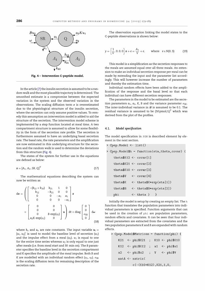
286 c o m p u t e r m e t h o d s a n d p r o g r a m s i n b i o m e d i c i n e 9 4 ( 2 0 0 9 ) 279–289
Fig. 4 – Intervention C-peptide model.
In the article [7] the insulin secretion is assumed to be a ran-dom walk and the most plausible trajectory is determined. Thesmoothed estimate is a compromise between the expectedvariation in the system and the observed variation in theobservations. The scaling diffusion term is overestimateddue to the physiological structure of the insulin secretion,where the secretion can only assume positive values. To rem-edy this assumption an intervention model is added to aid thestructure of the secretion. The intervention model scheme isimplemented by a step function located at meal time. A twocompartment structure is assumed to allow for some flexibil-ity in the form of the secretion rate profile. The secretion isfurthermore assumed to have an underlying basal secretionrate. The basal rate, the rate parameters and the amplificationare now estimated in this underlying structure for the secre-tion and the random walk is used to determine the deviationsfrom this structure (Fig. 4).
The states of the system for further use in the equationsare defined as below:
x = [A1, A2, SR, Q]T (17)
The mathematical equations describing the system cannow be written as
dx =
⎛⎜⎝⎡⎢⎣−(k12 + k10) k21 1 0
k12 −k21 0 00 0 −a1 a1
0 0 0 −a2
⎤⎥⎦x
+
⎡⎢⎣ 0 00 00 B exp(2)
a2K exp(1) 0
⎤⎥⎦u
⎞⎟⎠ dt + diag
⎡⎢⎣ 00
SR
0
⎤⎥⎦ dω
(18)
where kx and ax are rate constants. The input variable ut =[u1, u2]′ is used to model the baseline level of secretion (u1)and the impulse effect from a meal (u2). u1 is equal to onefor the entire time series whereas u2 is only equal to one justafter meals (i.e. from meal start and 30 min on). The B param-eter specifies the baseline level in the secretion compartmentand K specifies the amplitude of the meal impulse. Both B andK are modelled with an individual random effect (1, 2). SR
is the scaling diffusion term for remaining description of thesecretion rate.
The observation equation linking the model states to theC-peptide observations is shown below:
y =[
1V
, 0, 0, 0]
x + e = A1
V+ e, where e ∈ N(0, S) (19)
This model is a simplification as the secretion responses tothe meals are assumed equal over all three meals. An exten-sion to make an individual secretion response per meal can bemade by extending the input and the parameter list accord-ingly. This will however increase the number of parametersand thereby the estimation time.
Individual random effects have been added to the ampli-fication of the response and the basal level so that eachindividual can have different secretion responses.
The parameters in the model to be estimated are the secre-tion parameters a1, a2, K, B and the variance parameter SR.The inter-individual variance in ˝ is assumed to be 0.1. Theresidual variance is assumed to be (50 pmol/L)2 which wasderived from the plot of the profiles.
4.1. Model specification
The model specification in PSM is described element by ele-ment in the next section.
Initially the model is setup by creating an empty list. The h
function that translates the population parameters into indi-vidual parameters is specified. Function arguments that canbe used in the creation of phi are population parameters,random effects and covariates. It can be seen that four indi-vidual parameters are extracted from the covariates and thetwo population parameters K and B are expanded with randomeffects.

c o m p u t e r m e t h o d s a n d p r o g r a m s i n b i o m e d i c i n e 9 4 ( 2 0 0 9 ) 279–289 287
The first element created here is the time invariant matri-ces. In this example all four matrices need to be specified.First the individual parameters are extracted from phi andmatrices are set up in a list named Matrices.
The initial conditions for the states are added to the listas an element named X0. The initial conditions used here aresteady state conditions calculated using the basal secretionand kinetic parameters. The initial conditions are specified asa function with arguments Time, phi and U. The Time argu-ment is the first time point specified and can be useful ifthe subjects start at different time points. The U can containexogenous input to the system which enters into the initialconditions.
Table 7 – Estimated parameters.
Parameter MLE 95% CI
K 1911.2 [1511.5; 2310.9]B 7.019 [5.0; 9.037]a1 0.029 [0.022; 0.036]a2 0.011 [0.0089; 0.014]SIG33 30.3 [26.05; 34.55]
Fig. 5 – Fitted C-peptide concentrations for subject 11.
The diffusion scaling term and the residual variance arespecified using the elements SIG and S. Both are specified asfunctions of phi. It can be seen that SIG is a 4 × 4 matrix withonly an element at position [3, 3]. S is specified as a matrixeven though it is one-dimensional.
The final element in the model is the function that splitsthe parameter vector containing parameters to be optimizedinto population parameters and inter individual covariancematrix ˝.
The list Cpep.Model now contains all the elementsrequired in the model specification and the model can now beused to estimate parameters and create the smoothed profiles.
4.2. Results
The parameters in the C-peptide intervention model areestimated using PSM.estimate with constraints on theparameters. The optimal parameters and confidence bandsare shown in the Table 7.
Two model fits for C-peptide can be seen in Figs. 5 and 6. Theplots show the observations as circles and the intervention
Fig. 6 – Fitted C-peptide concentrations for subject 12.

288 c o m p u t e r m e t h o d s a n d p r o g r a m s i n b i o m e d i c i n e 9 4 ( 2 0 0 9 ) 279–289
Fig. 7 – Secretion for subject 11.
model fit is shown in blue. The dashed line represents thedeterministic model fit where the diffusion scale term hasbeen fixed to zero in the intervention model in order to mimican ODE model like in NONMEM. The dashed line is thus equalto a simulation with the intervention model.
The failure of the assumption of equal responses to allmeals is obvious in the fit between the dashed red line andthe observations. Large peaks are underestimated and smallpeaks overestimated. This is clear as the model describes theaverage response after a meal. The solution could be to extendthe model so that every meal has it’s own amplification.
As the model is used for deconvolution purposes the actualfit to the observations is of less importance, but more interest-ing is the secretion rate profile and the split between the modeland the Wiener component.
The two corresponding secretion rate profiles to the C-peptide fits are found in Figs. 7 and 8. The full line is theoptimal secretion rate determined by the Kalman Filter andthe dashed line represents the deterministic part of the model.The secretion model captures the overall trends but the com-promise with the equal response assumption is clear.
The deconvoluted insulin secretion rates have some jumpswhich seem unphysiological. The solution could be to usean integrated random walk as driver for insulin secretion.This would make the deconvoluted insulin secretion rate lesserratic.
This section has shown a simple application of the PSM
package for modelling purposes. Classic log likelihood ratiotesting can also be applied in the model development as wellas visual predictive checks of the model fits.
Fig. 8 – Secretion for subject 12.
5. Discussion and conclusion
The PSM package provides a new general framework forhandling dynamic models based on stochastic differentialequations in a population setting. The package is availablein R to ease availability, ease installation and enable a sin-gle working environment for data handling, modelling andvisualization.
The package is an extension to the Matlab framework ofthe same name. The package functionality is a combinationof the functionality available in CTSM and NONMEM. CTSMand NONMEM have also been used to validate the package asdescribed further on the homepage [16].
The package enables the feature of dosing capabilitieswhich makes the package useful in PK/PD model development.This is further supported by the ability to handle multidi-mensional observations which aids in modelling work withobservations from both PK and PD.
The package includes functionality for modelling taskssuch as simulation, parameter estimation and smoothing.The stochastic deconvolution example with an underlyingsecretion model in this article showed an application of thepackage.
The computational effort in working with larger models issubstantial and the use of parallelization could decrease thetime considerably in the modelling. It is currently being inves-tigated how to implement parallelization in a general mannerin R. Parallelization is an obvious solution due to the fact thatfuture computer systems will be massive multicore systems.
The package is a promising tool to get started with stochas-tic differential equations or the inclusion of mixed-effects incontinuous-discrete state-space models.
More information can be found on the webpage http://www.imm.dtu.dk/psm.
Acknowledgement
This work was supported by the European Union throughthe Network of Excellence BioSim, contract no. LSHB-CT-2004-005137.
r e f e r e n c e s
[1] N.R. Kristensen, H. Madsen, S.H. Ingwersen, Using stochasticdifferential equations for PK/PD model development, J.Pharmacokinet. Pharmacodyn. 32 (February(1)) (2005)109–141.
[2] C.W. Tornøe, R.V. Overgaard, H. Agersø, H.A. Nielsen, H.Madsen, E.N. Jonsson, Stochastic differential equations inNONMEM: implementation, application, and comparisonwith ordinary differential equations, Pharm. Res. 22(August(8)) (2005) 1247–1258.
[3] R.V. Overgaard, N. Jonsson, C.W. Tornøe, H. Madsen,Non-linear mixed-effects models with stochasticdifferential equations: implementation of an estimationalgorithm, J. Pharmacokinet. Pharmacodyn. 32 (February(1))(2005) 85–107.
[4] U. Picchini, S. Ditlevsen, A. De Gaetano, Maximum likelihoodestimation of a time-inhomogeneous stochastic differential

c o m p u t e r m e t h o d s a n d p r o g r a m s i n b i o m e d i c i n e 9 4 ( 2 0 0 9 ) 279–289 289
model of glucose dynamics, Math. Med. Biol. 25 (June(2))(2008) 141–155.
[5] L.B. Sheiner, S.L. Beal, NONMEM User’s Guide, NONMEMProject Group, University of California, San Francisco, 1994.
[6] N.R. Kristensen, CTSM Mathematics Guide, TechnicalReport, Technical University of Denmark, December 2003.
[7] S.B. Mortensen, S. Klim, B. Dammann, N.R. Kristensen, H.Madsen, R.V. Overgaard, A Matlab framework for estimationof NLME models using stochastic differential equations:applications for estimation of insulin secretion rates, J.Pharmacokinet. Pharmacodyn. 34 (October(5)) (2007)623–642.
[8] C.W. Tornøe, H. Agersø, E. Niclas Jonsson, H. Madsen, H.A.Nielsen, Non-linear mixed-effectspharmacokinetic/pharmacodynamic modelling in NLMEusing differential equations, Comput. Meth. ProgramsBiomed. 76 (October(1)) (2004) 31–40.
[9] R.E. Kalman, New approach to linear filtering and predictionproblems, Am. Soc. Mech. Eng. – Trans. – J. Basic Eng. Ser. D82 (1) (1960) 35–45.
[10] G. Welch, G. Bishop, http://www.cs.unc.edu/∼welch/kalman/.
[11] R.V. Overgaard, Pharmacokinetic/PharmacodynamicModeling with a Stochastic Perspective. Insulin Secretionand Interleukin-21 Development as Case Studies, PhDThesis, Technical University of Denmark, Informatics andMathematical Modelling, 2006.
[12] L.B. Sheiner, S.L. Beal, Evaluation of methods for estimatingpopulation pharmacokinetics parameters. I.Michaelis–Menten model: routine clinical pharmacokineticdata, J. Pharmacokinet. Biopharm. 8 (December(6)) (1980)553–571.
[13] T. Kailath, A.H. Sayed, B. Hassibi, Linear Estimation,Prentice-Hall, 2000.
[14] E. Van Cauter, F. Mestrez, J. Sturis, K.S. Polonsky, Estimationof insulin secretion rates from c-peptide levels comparisonof individual and standard kinetic parameters for c-peptideclearance, Diabetes 41 (March(3)) (1992) 368–377.
[15] N.R. Kristensen, A deconvolution method for linear andnonlinear systems based on stochastic differentialequations, Population Approach Group Europe, 2004.
[16] S. Klim, S.B. Mortensen, PSM homepage. Internet:http://www.imm.dtu.dk/psm, June 2008.

Appendix D
Paper D
Title:Local estimation of a discretely observed continuous time inhomogeneous markovjump process.
Authors:S. B. Mortensen, H. Madsen, and P. Hougaard.
Submitted to:Statistical Modelling (May 2009).

Local Estimation of a Discretely Observed
Continuous Time Inhomogeneous Markov
Jump Process
Authors: Stig B. Mortensen1,2,†, Henrik Madsen1 and Philip Hougaard2
1 DTU-Informatics, Technical University of Denmark, Lyngby, Denmark2 H. Lundbeck A/S, Valby, Denmark† Corresponding author: [email protected]
May 14, 2009
Abstract
A general estimation method for a discretely observed inhomogeneouscontinuous time Markov jump process is presented. The method is able tohandle time series data with a discrete sample space, where it is reasonableto assume that the data is generated by a slowly varying inhomogeneousMarkov jump process. The estimation method uses local kernel estima-tion in combination with a weighted log-likelihood model to capture timevariations of the Markov process. An application of the method is illus-trated on data of discretely sampled sleep stages from an EEG study onrats.
Keywords:Kernel estimation, maximum likelihood, Markov process, sleep EEG data.
Sumitted for:Statistical modelling (May 14, 2009).
1

1 Introduction
In many applications one may encounter discretely sampled data that has afinite sample space. Examples of such are financial data with credit ratings,observations of cloud cover or observations of sleep stages during human oranimal sleep. A first assumption for such data will often be that the data isgenerated by a time homogeneous Markov process. The homogeneous Markovassumption is often approximately valid over short time intervals, but if data issampled over longer time periods this may no longer be the case due to changesover time of the system. Relating to the above mentioned examples the causecould be new financial market conditions, changes of season and changes in thesleep process.
One way to handle such changes in the dynamics of the process is to applyan inhomogeneous continuous time Markov model. This is an attractive modelas it has a simple model structure but is still very flexible. Being inhomogeneousthe model is able to reflect changes in the system and by further formulatingthe model in continuous time will often allow a more simple parameterization ofthe model that can be related to physical constraints in the system. This papersuggests a novel estimation procedure that based on discrete measurements willestimate changes in the model parameters over time for the continuous Markovprocess.
The theory of the method is presented in Section 2 and 3 and in Section 4its application is illustrated with data from a study of EEG sleep stages in rats.
2 Model
Let X(t) ∈ S; t ∈ T be a continuous time inhomogeneous Markov process witha finite state space S = 1, ...,m and T = [0, tmax]. The process is defined bya stochastic matrix of transition probabilities P (t, u) = pij(t, u) with
pij(t, u) = PrX(u) = j|X(t) = i. (2.1)
By introducing the corresponding intensity matrix Q(t) = qij(t) it can beshown that
∂
∂uP (t, u) = P (t, u)Q(u), u, t ∈ T, (2.2)
which is known as the Kolmogorov forward differential equation. The equationshows that the process is also defined completely through the Q(t) matrix (Coxand Miller, 1965, p. 181). The Q(t) matrix has diagonal elements qii ≤ 0 andoff-diagonal elements qij ≥ 0, i 6= j, and the matrix will always be defined givena Markov process with a stochastic matrix P (t, u). It can be shown that if Q(t)is time invariant then times between jumps (holding times) are exponentiallydistributed and the diagonal elements qii(t) of Q(t) contains the negative rate
2

for leaving a state. The fraction −qij(t)/qii(t) is the probability of going tostate j when a jump from state i occurs. Consequently, the row sum of Q(t)is 0 since
∑j 6=i−qij/qii must be 1, meaning that the process must jump to a
state in S with probability one when a transition occurs.
The process X(t) is observed at N discrete time points that are chosen inde-pendent of the observed process. The model dynamics are assumed to be slowlyvarying relative to the time between observations. The observation sequenceis denoted xk and contains the state at time tk where k = 1, ..., N . Thereis no requirement of an equidistant sampling scheme, and therefore “missing”observations do not need to be handled separately.
3 Estimation
Given a set of observations we wish to find an estimate of Q(tc) at a timepoint tc ∈ T using a locally-weighted maximum likelihood frame work. Tofurther estimate the time variations ofQ(t) over the entire interval T one simplyapplies the local model sequentially for a series of suitably close time points inT . The presentation of the estimation method is thus only concerned with thepoint estimate Q(tc) the remaining part of the section. The dependence on thechosen time point tc is suppressed in the notation to ease readability, but it isimportant and should be kept in mind.
It will often be the case that the estimation of Q(t) should be limited to aparticular structure of interest. For this purpose we define in f a parameteriza-tion for the Q(t) matrix with a set of parameters θ(t) = (θ1(t), ... , θv(t)) suchthat
f : θ(t) → Q(t). (3.1)
The parameterization in (3.1) can be used to define a particular structure ofQ(t) based on a knowledge of the process. Thus instead of estimating the fullQ(t) matrix it is only nescessary to estimate the parameters representing possi-ble jumps in continuous time. This typically limits the number of parameters inQ(t) that has to be estimated. The parameterization in (3.1) can also be usedto define a more suitable transformation of the elements in Q(t) to be used inthe maximum likelihood estimation. The elements qij(t) are all rate relatedparameters and it may thus be desirable to estimate the logarithm of these tomake the parameter space unbounded.
Next, define in g a series of local polynomial models of order r for theparameters (θ1(t), ... , θv(t)) such that
g : (β, t) → θ(t) (3.2)
whereθs(t) = βs0 + (t− tc)βs1 + ... + (t− tc)rβsr (3.3)
3

with the matrix β = βkl , s = 1, ..., v and l = 0, ..., r. It then holds that alocal estimate of the Q(tc) matrix is given by Q(tc) = f(g(β, tc)), where β isan estimate of β. This estimate will be based on a locally-weighted likelihoodfunction, which will be described in the following.
First we define a series of stochastic matrices
P k = pijk = pij(tk, tk+1) (3.4)
containing the probabilities for observing xk+1 = j given xk = i. These transi-tion probabilities are found by solving (2.2) with initial condition P (tk, tk) = Iand using Q(u) = f(g(β, u)). The solution can be found numerically usingstandard algorithms for solving ordinary differential equations. Alternatively,if the time interval ∆tk = tk+1 − tk is small, one may as an approximation usea zero or first order Taylor expansion of Q(t) around tk. The most simple andin many cases sufficient approximation is the zeroth order expansion where theintensity matrix is assumed constant in each time interval tk to tk+1. In thiscase the solution to (2.2) is given explicitly as
P k = exp[Q(tk) ∆tk ]= exp[f(g(β, tk))∆tk ] (3.5)
where exp[·] represents the matrix exponential function. This approximation iscomputationally faster, and will in many cases be sufficiently accurate as longas the time variations in Q(t) are small compared to the time interval betweenconsecutive observations.
In order to simplify the description of the likelihood function for β an indica-tor observation yijk is defined from xk with i, j = 1, ...,m and k = 1, ..., N−1.Let yijk = 1 when xk = i and xk+1 = j and otherwise yijk = 0 . The obser-vation yijk thus indicates if a change of state from i to j is observed from timetk to tk+1. This new set of indicator observations contains all the informationin the original set of observations xk and is thus also a sufficient statistic forestimating β. Using the transition probabilities defined in (3.4) we know thatthe likelihood of observing xk = i followed by xk+1 = j is pijk. The contributionto the log-likelihood for one observation yijk can thus be written as yijk log pijk
and combining all m2 indicator observations at time tk this gives
log Lk(β) =∑
i
∑j
yijk log pijk(β). (3.6)
We now define weights for the observations as wk(tc) = Kh(tk − tc) using asymmetric probability function K (also often referred to as a kernel function).The parameter h is the bandwidth controlling the size of the local neighborhoodsuch that Kh(t) = K(t/h)/h (Fan and Gijbels, 1996, p. 15). This can be used
4

to form a locally weighted log-likelihood function for β as
log L(β, tc) =∑
k
wk(tc) log Lk(β) (3.7)
=∑
k
∑i
∑j
wk(tc) yijk log pijk(β) (3.8)
and β may thus for a given time point tc be estimated locally as
β = arg maxβ
log L(β, tc). (3.9)
Given that the local polynomia in (3.3) are centered around tc, a local esti-mate of each parameter θs(tc) for a given tc is directly βs0. The estimate of allparameters in Q(tc) is thus given as
θ(tc) = g(β, tc) = β0
= [ β10, β20, ... , βv0 ].
3.1 Local constant model
The estimation method can be simplified if sample times are equidistant withtk = t1 + (k− 1)∆tk and if it is chosen to use a local constant model instead ofa higher order polynomial.
Thus, if we in (3.3) let r = 0 such that θs(t) = βs0 then Q(t) modelled asf(g(β, t)) will be constant with respect to t for a given β and the transitionprobabilities can be found using the matrix exponential in (3.5) without ap-proximation. Note that when using a local constant model in (3.3) the estimateQ(tc) is still varying with respect to tc due to the weighing of the observa-tions that depend on tc. Assuming equidistant sampling times then also ∆tkwill be constant, and this results in time invariant transition probabilities for agiven β. It is therefore only necessary to solve (2.2) one time instead of N − 1times to evaluate the likelihood function for β and we may write the transitionprobabilities pijk(β) as pij(β) for any k to emphasize this.
By defining a “weighted” number of jumps from i to j as n′ij =
∑k wk(tc) yijs
the locally-weighted log-likelihood function in (3.8) can be written as
log L(β, tc) =∑
k
∑i
∑j wk(tc) yijk log pijk(β)
=∑
i
∑j log pij(β)
∑k wk(tc) yijs
=∑
i
∑j log pij(β) n′
ij ,
(3.10)
where the sum over all observations is removed from the log-likelihood function.This formulation of the estimation problem gives a significant computational
5

advantage. The matrix n′ij can be pre-computed for a given tc since it does not
depend on β and an evaluation of the log-likelihood function then only requiressolving (2.2) once to compute pij(β). This not only reduces time requiredfor estimation, but also improves the numeric stability of the log-likelihoodevaluation.
3.2 Bias vs. variance of estimate
The local estimation method provides a point estimate of the parameters θ(tc)defining Q(tc) via the parameterization given in f . For any local estimationprocedure there will be a trade-off between reducing bias and variance of thispoint estimate.
To find an estimate of the variance we may rely on the asymptotic distri-bution theory of the maximum likelihood estimator, since the local estimationmethod is based on a likelihood function (Pawitan, 2001). The observed Fisherinformation for β0(tc) is
I0(tc) = − ∂2
∂β20
log L(β, tc)∣∣∣β0=β0
(3.11)
and using that θ(tc) = β0(tc) it thus holds asymptotically that
var θ(tc) = I−10 (tc). (3.12)
if θ(tc) is unbiased. From likelihood theory it is known that the variance esti-mate in (3.12) will decrease for an increasing bandwidth, since this will includemore observations in the likelihood function. However, θ(tc) will only be unbi-ased if the local model is correct on a global level, and this can generally not beassumed. The polynomial model is chosen because it is well suited for locallymodelling a true function of any any shape. If the bandwidth is increased tomuch this will no longer be the case and the decreasing variance will come atthe cost of increasing bias. The bandwidth should thus not be increased beyonda range where the polynomial approximation is expected to be sufficient andthe variance estimate in (3.12) should only be seen as a an indication of theprecision of the estimate in situations where bias is expected to be relativelysmall.
For local estimation in a least square setting (also known as non-parametricregression) with a model of the type zk = g(tk) + εk the problem of balanc-ing bias and variance in estimation of the unknown regression function g has along history. Classical methods for finding an optimal bandwidth include crossvalidation criterion and related methods (Wahba and Wold, 1975; Rice, 1984;Muller, 1985; Muller et al., 1987). With cross validation we define a cross valida-tion function CV (λ) = 1
n
∑k (zk − g∗λ(tk))2 where g∗λ(tk) is the non-parametric
estimate of g(tk) using all observations except observation zk. The parameter
6

λ is the reciprocal of the bandwidth, and minimizing the cross validation func-tion with respect to λ gives an objective choice of the optimal bandwidth. Thecross validation criterion can be generalized to other types of responses usingthe theory of generalized linear models where deviance is introduced to measureagreement between observations and model (McCullagh and Nelder, 1983). Ifwe assume a Gaussian distribution of εk and use µk = g(tk) the deviance for oneobservation is defined as D(zk, µk) = (zk−µk)2. In this way the cross validationfunction can be defined as CV (λ) = 1
n
∑k D(zk, µ∗
k) where D is the individualdeviance contribution for observation zk and µ∗
k = g∗λ(tk). In this form the crossvalidation technique can be extended to all types of responses in the exponentialfamily distribution (O’Sullivan et al., 1986) and this also includes the binaryobservations yijk of a Markov process presented here.
For binary observations it can be shown that the deviance is equal to minus2 log-likelihood of the binary observation. For the indicator observations yijk
we are only interested in the deviance contribution when yijk = 1 since thisindicates an actual observation. The deviance can thus be defined as
D(yijk, pijk) = −2yijk log pijk.
This can be used for defining a cross validation criterion as
CV (λ) =2n
∑i
∑j
∑k
−yijk log p∗ijk
where p∗ijk is found using a bandwidth h = 1/λ and excluding observation yijk.The cross validation criterion gives an objective measure for the optimal band-width in the local Markov model. The criterion will however quickly becomecomputationally demanding to evaluate with increasing number of observations,since it requires a local estimate p∗ijk at each time point tk to evaluate CV (λ).In practical situations it is thus only feasible to compute if the number of ob-servations is relatively small.
In problems where the number of observations is large as in the examplepresented in Section 4 other approaches are needed. Instead the situation canbe seen in analogy to estimation of the spectral density function in time seriesanalysis, where it is well known that some degree of smoothing is nescessaryto achieve a consistent estimate (Priestley, 1981). The degree of smoothing ischosen such that it seems to reasonably balance bias and variance. The sameapproach is suggested here, that is simply to redo the local estimation methodfor a range of bandwidth values to find the most suitable value.
3.3 Type of bandwidth and kernel function
The type of bandwidth and kernel function K is also important in order toachieve the best performance of the local estimation. There are a number of
7

commonly used kernel functions available, such as the Gaussian kernel, tricubekernel and the uniform, Epanechnikov, biweight and triweight kernels that arederived from the symmetric Beta family (Fan and Gijbels, 1996). A number ofthe kernels are shown in Figure 1. The Gaussian kernel has the disadvantageof unbounded support and hence positive weights for all data points. Thismakes the local estimation procedure computationally more demanding, sinceall data has to be considered at any chosen time point tc. The remaining kernelfunctions have only bounded support in the interval [−1; 1] which is mapped tothe interval [−h;h] in the scaled kernel function Kh. The tricube kernel is oftenpreferred because it approaches its bounds smoothly.
−2.0 −1.5 −1.0 −0.5 0.0 0.5 1.0
0.0
0.5
1.0 tricubeEpanechnikovuniformGauss
Figure 1: Kernel functions.
As discussed in the previous section a smaller bandwidth reduces estimationbias but increases the variance and vice versa. Two types of bandwidth havebeen considered here.
The first type of bandwidth is to use a common fixed bandwidth h. This isthe most simple way of specifying the bandwidth. It can be useful in many cases,but it can give large differences in the precision of the parameter estimates overtime. This happens if the observations are sampled with varying frequency andthereby results in varying numbers of observations in the fixed length intervalstc + [−h;h]. The fixed bandwidth h must naturally be positive, but it is notupwards bounded as increasing h just results in an increasingly smooth estimateof the time variations.
The second choice for a bandwidth is to choose a data dependent bandwidthhtc
such that the interval tc + [−htc;htc
] always includes a fixed proportion αof the total number of observations. This is often denoted a nearest neighbor(NN) bandwidth. The definition can be extended to allow α > 1 by scalinghtc
by max(1, α). The nearest neighbor bandwidth will help control estimationvariance when the frequency of observations varies.
If sample times are equidistant the two types of bandwidths are almost equiv-alent, since a fixed time window contains a fixed proportion of the data. Theywill only be different near the boundary, where the data dependent bandwidthincreases to contain the fixed proportion of the data. It is noted that for both
8

choices of bandwidth, when h →∞ or α →∞ the local estimation will approacha global polynomial estimation.
There are further aspects that can be considered when choosing kernels andbandwidth. For local estimation in a least square setting the estimation nearthe boundary (when tc < h or tc > tmax − h) can give problems with increasedbias. A common way to avoid this is to use special boundary kernels, see e.g.Gasser et al. (1985). Similar approaches could also be considered in this contextto improve the estimate at the boundary.
A special issue that in only relevant for the local estimation presented hereis that a chosen bandwidth must contain observations of all states in order toestimate all parameters in the model. If a particular state in the process isobserved much less frequently than other states, this will set a lower bound onthe possible bandwidth. A way to give more robust local estimates is thus to usea state dependent bandwidth such that e.g. a proportion α of the observationsof each state is included in the estimation. This can be done by using statedependent weights wik(tc) instead of wk(tc) in (3.8) where wik(tc) is found witha different bandwidth depending on from which state the observed jump yijk
occurs.
4 Example
To illustrate the use of modelling based on local estimation of a continuoustime inhomogeneous Markov process, the method will be applied to data froma study monitoring the sleep cycle of rats.
The data has been collected in a pre-clinical trial using 6 rats that havebeen observed for 23.5 hours (Anderson et al., 2005). At the beginning ofthe period the rats were given an oral dose of 20mg Gaboxadol, which is asleep promoting compound. Previous experience has indicated that the drugis present in the brain for about 8 hours and reaches the highest concentrationafter approximately 1 hour. During the first 12 hours the lights were on, and inthe remaining time the lights were off. Since rats are most active in the dark,this study design is meant to resemble a human taking a sleep drug before bedtime.
The sleep cycle is monitored using electroencephalography (EEG) which isused to determine the sleep stage of the rat. Three states are classified, namelywake (W), delta sleep (DS) and paradoxical sleep (PS) and the states are num-bered in that order. These states are determined every 10 seconds giving 8,460equidistantly spaced observations for each rat. In order to simplify the exampleit is chosen to regard the observations from all six rats as realizations of thesame Markov process. The local estimation thus reflects an average individualprocess.
9

The implementation of the estimation method has been done in R (R De-velopment Core Team, 2008) and it was chosen to use the matrix exponentialin (3.5) to solve (2.2) since data is sampled at high frequency compared to theexpected variations it Q(t). The matrix exponential is not part of base R so itwas chosen to use the Fortran routine DGPADM from Expokit (Sidje, 1998) forthis purpose.
The parameterization f of the Q(t) matrix is shown in (4.1). The structureis based on Madsen et al. (1985), where Q(t) is parameterized with two param-eters for each state, one rate parameter for leaving the state and one parameterfor the probability of changing one state down when a jump occurs. This param-eterization is advantageous if it is only possible to jump to neighboring states,since the number of parameters only increases linearly with the number of statesinstead of quadratically when using a full matrix. In this example we will usethe model
f : θ(t) → Q(t) :
Q(t) =
−q1(t) q1(t) 0w2(t)q2(t) −q2(t) (1− w2(t))q2(t)
(1− w3(t))q3(t) w3(t)q3(t) −q3(t)
qi(t) = exp[θi(t)], i = 1, 2, 3wi(t) = logit−1[θi+2(t)], i = 2, 3 ,
(4.1)
which is illustrated in Figure 2. Since the rats have only three states, the struc-ture with two parameters per state does not reduce the number of parametersneeded, but it is still used to illustrate the use of the approach.
W1
DS2
PS3
λ1 λ2 w2 , λ3 w3 ,
Figure 2: Model for sleep stage transitions.
In the parameterization in (4.1) we furthermore use the constraint thatw1(t) = 0 meaning that jumps from W to PS should never occur. This re-flects that it is known from physiology that the PS state is always preceded bythe DS state. There is a very small number of observations in the data where Wis followed by an observation of PS, but by using w1(t) = 0 we thereby assumethat the process has been in the DS state in between observation times.
For the local estimation we use a second order polynomial in g and a tricubekernel with a nearest neighbor bandwidth of α = 0.40. The result of the esti-mation is shown in Figure 3 together with Wald 95% confidence intervals foundusing (3.12).
10

Min
utes
0.00.51.01.52.02.53.03.5
0 6 12 18 24
E(W) = 1/q1
Min
utes
01234567
0 6 12 18 24
E(DS) = 1/q2
Min
utes
0.0
0.1
0.2
0.3
0.4
0 6 12 18 24
E(PS) = 1/q3
prob
abili
ty
0.0
0.2
0.4
0.6
0.8
1.0
0 6 12 18 24
w1: W −> PS
prob
abili
ty0.0
0.2
0.4
0.6
0.8
1.0
0 6 12 18 24
w2: DS −> W
prob
abili
ty
0.0
0.2
0.4
0.6
0.8
1.0
0 6 12 18 24
w3: PS −> DS
Figure 3: Estimate of the Q(t) matrix as a function of time using 2nd order localpolynomials and a NN bandwidth α = 0.40. The surrounding lines are Wald 95%pointwise confidence intervals.
The first row in Figure 3 shows the expected time in each state before leav-ing (holding times), which is found as 1/qi(t) since the time in each state isapproximately exponentially distributed. Looking at holding times is chosenhere since it can be a more intuitive way to view the rate parameters, but it isonly valid if the holding times are short compared to the time variations of theparameters as discussed previously. It is seen that the estimate of time in Wincreases after 12 hours (lights off) along with the probability of jumping fromDS to W when leaving DS, and this seems reasonable as the activity shouldincrease in the dark period. The expected time in DS reflects the influence ofthe drug, as it peaks at about three hours, which indicates a delay of 2 hourswith respect to the peak of the drug concentration. The most notable effect onthe pointwise confidence intervals is seen for w3 between 0 and 6 hours. Thisreflects that there is only limited information about the probability of goingfrom PS to DS or W, since the process only rarely enters the PS state in thisperiod as seen in the figure for 1/q3.
In the example shown in Figure 3 the estimation is done using a secondorder polynomial with an NN bandwidth α = 0.40. To demonstrate the effectof using lower orders, this is done for the DS state and shown in Figure 4(a)for the interval 0 to 18 hours. Both the zero and first order approximationsare expected to give negative bias around peaks, and this is seen clearly fromthe figure around the peak at 2-3 hours. For the later times in the interval 6to 18 hours the three approximations perform equally well. In Figure 4(b) thebandwidth is further reduced to α = 0.30. This gives increased sensitivity andthe second order local model is here seen to capture a stronger peak, whichfurther strengthen the evidence for a true significant increase in the expectedtime in DS is present. It has been tried to use an even lower bandwidth, butunfortunately the estimation of especially w3 becomes unstable. This is due
11

to a very limited number of observations of the PS state during the first hoursof the study, and for lower choices of bandwidth the estimation was no longerpossible. To further reduce the bandwidth it is nescessary to consider a statedependent bandwidth as mentioned in Section 3.3.
Min
utes
0
2
4
6
8
0 6 12 18
order 0order 1order 2
(a) α = 40%
Min
utes
0
2
4
6
8
0 6 12 18
order 0order 1order 2
(b) α = 30%
Figure 4: Expected time in DS state for different order of local polynomial using twochoices of NN bandwidths.
It is also of interest to get an impression of whether the Markov assumptionis valid. As noted earlier the holding times should be exponentially distributedwhen the Markov process is homogeneous. Based on Figure 3 it can be seenthat the process can be assumed to be roughly homogeneous in the time between14 and 22 hours. Since data are sampled equidistantly the distribution of theobserved holding time follows a geometric distribution. It is chosen to lookat the run lengths as this is proportional to the observed holding times. Thedistribution of the run lengths K is given as
Pr(K = k) = pk−1ii (pii − 1), k ∈ N, (4.2)
where pii is the (assumed constant) probability of staying in the same state. Theobserved distribution of the run lengths can be seen in Figure 5. This histogramis shown on log-scale, so it is expected to show a straight line. The solid lineis the expected distribution based on p = nii/ni·, i.e. the observed number ofjumps from state i to state i divided by total number of jumps from state i. Itis seen that the overall picture is reasonable, but for both Wake and Delta Sleepthere seems to be too many long runs compared to the linear decline in the firstpart of the histogram.
5 Discussion
We have presented a method for analyzing time series data with a discretesample space based on the assumption data is generated by a continuous timeinhomogeneous Markov jump process. A first objection to this choice of model
12

1 20 40 60
12
51020
50100200
(a) Wake
1 20 40 60
12
51020
50100200
(b) Paradoxical
1 20 40 60
12
51020
50100200
(c) Delta Sleep
Figure 5: Histogram of run lengths for data between 14 and 22 hours.
could be: why assume a model in continuous time when data is sampled dis-cretely? In particular when data is sampled equidistantly as in the example inSection 4 it could seem appealing to instead assume a discrete Markov process.
The first answer is that if the process is in fact evolving in continuous time isshould also be modelled as such. An example is the observation of sleep cyclesfrom the previous section which is most naturally understood as a continuousprocess. Also e.g. the example of observations of cloud cover mentioned in theintroduction is by nature a continuous process. It is only due to the physicallimitations that we are forced to consider discrete observations of the processes.
When the model is handled in continuous time it allows us to apply con-straints to the parameterization. This is used in the model for the sleep datain (4.1) where jumps between W and PS are restricted. Another example isfound in Madsen et al. (1985) where data from observations of cloud cover isanalyzed using a continuous time Markov model. On a short time scale it isknown that the weather conditions cannot jump from few to many clouds – theprocess must visit all stages in between seen on a continuous time scale. Thisallows a parameterization of the Q(t) matrix where only jumps to neighboringsstates are possible. If the same process were analyzed in discrete time such aconstraint could not be applied, since observations of jumps between all statesbecomes probable. Constraining jumps to neighboring states is only valid inthe limit when the time step approaches zero, and this limit is the continuousrepresentation of the model.
The continuous time model also gives a more natural parameterization of theprocess, where rates or holding times are estimated instead of probabilities. Formost people it is more natural to look at the expected holding time for a stateinstead of the probability for leaving at the next observation time. Of coursethese two quantities are to some extent equivalent, and the relation in (3.5) couldsuggest that one could simply find the continuous representation by solving theequation P t = exp(Q(t)∆t) for Q(t) for a given estimate of P t. However,this equation will not always have a solution due to the imbedding problem for
13

Markov chains (Bladt and Sørensen, 2005). In general terms the problem willarise in cases where the process moves to fast between states compared to thesampling rate. This is in fact the case in the sleep example data (Section 4)due to the PS state, which has very short holding times. The problem with theimbedding problem for Markov chains are only avoided by doing the estimationdirectly in continuous time.
In the formulation of the inhomogeneous Markov model it is assumed thatthe model dynamics are slowly varying. This formulation does not include aprocess that has discontinuities in model parameters as a function of time. Itcould be argued that such a discontinuity is present in the sleep data when lightsare turned on after 12 hours. The smooth change in the parameters around12 hours seen in Figure 3 is thus only an effect of averaging data from bothsides of this discontinuity. However, if the estimation around a discontinuity isof particular interest it can be accommodated using standard techniques fromlocal estimation. Either it can be chosen to use a smaller bandwidth where adiscontinuity is suspected, or one could choose to use a type of boundary kernel,such that data on one side is not used in the estimation on the other side.
To summarize, the proposed estimation method is aimed at analyzing timeseries data with a discrete sample space by assuming an inhomogeneous Markovmodel in continuous time. The formulation of the model in continuous timecan reduce the number of parameters in the model by introducing constraintson jumps that exist in the physical system. The estimation method makes itpossible to make local non-parametric estimates of changes in model parametersas a function of time. Such changes in the model dynamics can otherwise easilybe overlooked or ignored by assuming a homogeneous Markov model, but asillustrated with the sleep data example it can provide valuable information aboutthe underlying process.
References
Anderson, N., S. Garson, S. Fox, S. Doran, B. Ebert, and J. Renger (2005,November). Investigation of effect of route of administration on gaboxadolinduced changes in arousal state and eeg parameters. H. Lundbeck A/S.
Bladt, M. and M. Sørensen (2005). Statistical inference for discretely observedmarkov jump processes. Journal of the Royal Statistical Society Series B67 (3), pp. 395–410.
Cox, D. R. and H. D. Miller (1965). The Theory of Stochastic Processes.Methuen & Co Ltd.
Fan, J. and I. Gijbels (1996). Local Polynomial Modelling and Its Applications:Monographs on Statistics and Applied Probability 66. Chapman & Hall.
14

Gasser, T., H.-G. Muller, and V. Mammitzsch (1985). Kernels for nonparametriccurve estimation. Journal of the Royal Statistical Society Series B 47 (2), pp.238–252.
Madsen, H., H. Spliid, and P. Thyregod (1985). Markov models in discrete andcontinuous time for hourly observations of cloud cover. Journal of AppliedMeteorology 24 (7), pp. 629–639.
McCullagh, P. and J. A. Nelder (1983). Generalized Linear Models. Chapmal& Hall.
Muller, H.-G. (1985). Empirical bandwidth choice for nonparametric kernelregression by means of pilot estimators. Statistics and Decisions, SupplementIssue(2), pp. 193–206.
Muller, H.-G., U. Stadtmuller, and T. Schmitt (1987). Bandwidth choice andconfidence intervals for derivatives of noisy data. Biometrika 74 (4), pp. 743–9.
O’Sullivan, F., B. S. Yandell, and W. J. Raynor (1986). Automatic smoothingof regression functions in generalized linear models. Journal of the AmericanStatistical Association 81 (393), pp. 96–103.
Pawitan, Y. (2001). In All Likelihood: modelling and inference using the likeli-hood. Oxford University Press.
Priestley, M. B. (1981). Spectral Analysis and Time Series, Volume 1. AcademicPress.
R Development Core Team (2008). R: A Language and Environment for Statis-tical Computing. Vienna, Austria: R Foundation for Statistical Computing.ISBN 3-900051-07-0.
Rice, J. (1984). Bandwidth choice for nonparametric kernel regression. TheAnnals of Statistics (4), pp. 1215–30.
Sidje, R. B. (1998). Expokit. A software package for computing matrix expo-nentials. ACM Transactions on Mathematical Software 24 (1), pp. 130–156.
Wahba, G. and S. Wold (1975). A completely automatic french curve: fittingspline functions by cross-validation. Communications in Statistics 4, pp. 1–17.
15
Appendix E
Paper E
Title:Flexible estimation of nonlinear mixed models via Laplace’s approximation.
Authors:S. B. Mortensen and R. H. B. Christensen.
Submitted to:The Journal of Computational and Graphical Statistics (September 2009).

Flexible Estimation of Nonlinear Mixed Models via
the Multivariate Laplace Approximation
Stig Bousgaard Mortensen1,2 &
Rune Haubo Bojesen Christensen1
September 20, 2009
1Informatics and Mathematical Modelling, Technical University of Denmark,
2800 Lyngby, Denmark. 2E-mail: [email protected]
Abstract
The multivariate Laplace approximation to the marginal likelihood is a fast
and accurate approach for estimation in nonlinear mixed models. Our aim is to
show how this approximation is easily implemented on a case-by-case basis in
general programming environments such as R, S-plus or Matlab. The approach
is very flexible compared to what is possible in standard statistical software
allowing estimation of models with e.g. crossed random effects and arbitrary
correlation structures for the residuals. Such models are not easily, if at all
possible, fit with standard statistical software or software specially designed for
nonlinear mixed models. The approach also allows graphical assessment of suc-
cessful convergence and can produce profile likelihoods for selected parameters,
neither of which is generally possible with standard statistical software.
Keywords: Crossed random effects, orange tree data, R.
1 Introduction
This paper is concerned with estimation of nonlinear mixed models (NLMMs) where
the conditional distribution of the response given the random effects as well as the
distribution of the random effects are Gaussian. The model can be expressed generally
as
(Y |B = b) ∼ N(f (β, b),Σ(λ)), B ∼ N(0,Ψ(ψ)), (1)
1

where β are fixed regression parameters, b is a q-vector of random effects, λ and
ψ are variance parameters parameterizing the covariance matrices Σ and Ψ and f
is the model function. NLMMs can be viewed as a generalization of the ordinary
fixed effects nonlinear model (NLM) (Bates and Watts, 1988) to include random
effects, and it can be viewed as a generalization of the linear mixed model (LMM)
(Laird and Ware, 1982) to allow the conditional mean to be a nonlinear function
of the regression parameters. Despite these conceptually small changes, maximum
likelihood estimation in NLMMs has been a fair challenge and still is to some extent.
The likelihood function of a NLMM is the marginal density of the response where the
random effects are integrated out
L(θ;y) =
∫Rq
p(y|θ, b)p(b) db, (2)
where p denotes a normal probability density function and θ = [βT ,λT ,ψT ]T denotes
the vector of fixed parameters. It is this q-dimensional integral that is difficult to
solve in general, because approximations have to be invoked. The likelihood can be
reduced to a multiple of integrals of lower order when the random parameters arise
from only one level of grouping (indexed by i, say); the model can be written as
(Yi|Bi = bi) ∼ N(fi(β, bi),Σi), Bi ∼ N(0,Ψ), i = 1, . . . , M,
and the likelihood simplifies to a multiple of qi-dimensional integrals
L(θ;y) =M∏i=1
∫Rqi
p(yi|θ, bi)p(bi) dbi,
where qi is the number of random effects for the ith group. In particular, the likeli-
hood reduces to a multiple of one-dimensional integrals when only a single random
effect occurs for each group in the data. We will refer to a set of random effects
corresponding to a single grouping variable as a random component.
In this paper we shall be concerned with the multivariate Laplace approximation
to solve the full q-dimensional integral (2) and thereby allow for any structure of the
random effects: scalar or vector-valued random effects, nested, crossed or partially
crossed; linear, as well as nonlinear.
Pinheiro and Bates (1995) and Vonesh (1996) studied the Laplace approximation
(Barndorff-Nielsen and Cox, 1989; Tierney and Kadane, 1986) for models with a
single level of grouping, and Pinheiro and Bates (2000) also studied it for models
with nested random effects. Statistical software packages that fit NLMMs (e.g. nlme
in R and S-plus (Pinheiro et al., 2008), SAS NLMIXED (SAS Institute Inc., 2004)
2
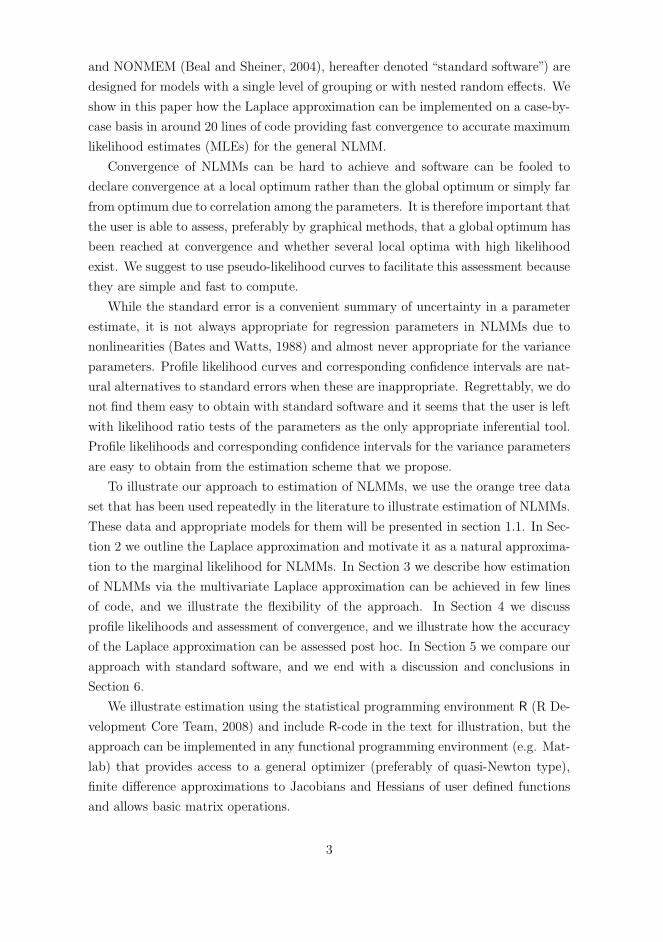
and NONMEM (Beal and Sheiner, 2004), hereafter denoted “standard software”) are
designed for models with a single level of grouping or with nested random effects. We
show in this paper how the Laplace approximation can be implemented on a case-by-
case basis in around 20 lines of code providing fast convergence to accurate maximum
likelihood estimates (MLEs) for the general NLMM.
Convergence of NLMMs can be hard to achieve and software can be fooled to
declare convergence at a local optimum rather than the global optimum or simply far
from optimum due to correlation among the parameters. It is therefore important that
the user is able to assess, preferably by graphical methods, that a global optimum has
been reached at convergence and whether several local optima with high likelihood
exist. We suggest to use pseudo-likelihood curves to facilitate this assessment because
they are simple and fast to compute.
While the standard error is a convenient summary of uncertainty in a parameter
estimate, it is not always appropriate for regression parameters in NLMMs due to
nonlinearities (Bates and Watts, 1988) and almost never appropriate for the variance
parameters. Profile likelihood curves and corresponding confidence intervals are nat-
ural alternatives to standard errors when these are inappropriate. Regrettably, we do
not find them easy to obtain with standard software and it seems that the user is left
with likelihood ratio tests of the parameters as the only appropriate inferential tool.
Profile likelihoods and corresponding confidence intervals for the variance parameters
are easy to obtain from the estimation scheme that we propose.
To illustrate our approach to estimation of NLMMs, we use the orange tree data
set that has been used repeatedly in the literature to illustrate estimation of NLMMs.
These data and appropriate models for them will be presented in section 1.1. In Sec-
tion 2 we outline the Laplace approximation and motivate it as a natural approxima-
tion to the marginal likelihood for NLMMs. In Section 3 we describe how estimation
of NLMMs via the multivariate Laplace approximation can be achieved in few lines
of code, and we illustrate the flexibility of the approach. In Section 4 we discuss
profile likelihoods and assessment of convergence, and we illustrate how the accuracy
of the Laplace approximation can be assessed post hoc. In Section 5 we compare our
approach with standard software, and we end with a discussion and conclusions in
Section 6.
We illustrate estimation using the statistical programming environment R (R De-
velopment Core Team, 2008) and include R-code in the text for illustration, but the
approach can be implemented in any functional programming environment (e.g. Mat-
lab) that provides access to a general optimizer (preferably of quasi-Newton type),
finite difference approximations to Jacobians and Hessians of user defined functions
and allows basic matrix operations.
3

The complete R-code to produce all fits and figures can be downloaded from
http://imm.dtu.dk/~sbm/nlmm/.
1.1 The orange tree data set and appropriate models
To illustrate our approach to estimation of NLMMs, we use a study of the growth of
orange trees reported by Draper and Smith (1981, p. 524), see the appendix, where
the circumference of five trees is measured at seven time points. This data set has been
used by Lindstrom and Bates (1990) to illustrate their algorithm, by Pinheiro and
Bates (1995) in their comparison of estimation methods and in Wolfinger (1999) to
illustrate the NLMIXED procedure. A logistic growth model is fitted in all cases with
a single random component bi allowing for a tree specific asymptotic circumference
yij =β1 + bi
1 + exp[−(tj − β2)/β3]+ ǫij , i = 1, ..., 5, j = 1, ..., 7, (3)
with ǫij ∼ N(0, σ2) and bi ∼ N(0, σ2b ) and mutually independent. The matrices Σ
and Ψ are both diagonal. Here, β1 determines the asymptotic circumference, β2 is
the age at half this value, β3 is related to the growth rate and tj is the time in days
since the beginning of the study. The maximum likelihood estimates (MLEs) of the
fixed parameters along with standard errors for model (3) are given in Table 1. A
plot of the data and model (3) is shown in Figure 1(a).
Table 1: Parameter estimates (standard errors) and log-likelihoods for models esti-mated in section 3.2 for the orange tree data.
Model β1 β2 β3 β4 σ σb1 σb2 ρ log(L)(3) 192.1 727.9 348.1 7.84 31.6 -131.57
(15.7) (35.3) (27.1)(4) 196.2 748.4 352.9 5.30 32.6 10.5 -125.45
(19.4) (62.3) (33.3)(5) 217.1 857.5 436.8 0.322 4.79 36.0 -116.79
(18.1) (42.0) (24.5) (0.038)(4) + (6) 192.4 730.1 348.1 6.12 32.7 12.0 0.773 -118.44
(19.6) (63.8) (34.2)(5) + (6) 216.2 859.1 437.8 0.330 5.76 36.7 0.811 -106.18
(17.6) (30.5) (21.6) (0.022)
A plot of residuals versus time (sampling occasion) shown in Figure 1(b) reveals
an unmodeled variation with time as is also noted by Millar (2004). Millar proposes
to include a second random component, b2j for the sampling occasion, that is, crossed
4

0 500 1000 1500
050
100
150
200
Days since 31 Dec 1968
Tru
nk c
ircum
fere
nce
(mm
)
Tree 1Tree 2Tree 3Tree 4Tree 5
(a) Orange tree data and model fit.
Res
idua
ls (
mm
)
−15
−10
−5
0
5
10
15
Apr
−28
Apr
−28
Apr
−28
Apr
−28
Apr
−28
Apr
−29
Apr
−29
Apr
−29
Apr
−29
Apr
−29
Oct
−26
Oct
−26
Oct
−26
Oct
−26
Oct
−26
Oct
−01
Oct
−01
Oct
−01
Oct
−01
Oct
−01
May
−15
May
−15
May
−15
May
−15
May
−15
Oct
−03
Oct
−03
Oct
−03
Oct
−03
Oct
−03
May
−01
May
−01
May
−01
May
−01
May
−01
’70 ’71 ’72 ’73
(b) Residuals versus time.
Figure 1: Plots for model (3) for orange tree data.
with the random component for trees. He suggests the model
yij =β1 + b1i + b2j
1 + exp[−(tj − β2)/β3]+ ǫij (4)
with b2j ∼ N(0, σ2b2) and independent of b1i and ǫij , which successfully removes the
most significant structure in the residuals. In this model, the effect of the sampling
occasion, b2j is proportional to the model prediction. This is reasonable during the
initial growth period, but unreasonable when the trees reach their asymptotic circum-
ference. Rather, we find it more natural to include b2j additively in the exp-term in
the denominator in model (3) to make the random effects additive on the logit-scale.
This makes the effect of the sampling occasion vanish as the trees approach their
asymptotic circumference.
A closer look at the sampling scheme reveals, however, that the apparently random
effect of the sampling occasion is caused by a seasonal effect and an irregular sampling
pattern. In the residual plot in Figure 1(b), it is seen that all samples are taken either
in the spring (April or May) or in the fall (October) and that two periods are missing.
We include a categorical seasonal effect, β4 such that
yij =β1 + b1i
1 + exp[−((tj − β2)/β3 + sjβ4)]+ ǫij (5)
where sj is −1/2 and 1/2 for samples taken in the spring and fall respectively. The
models (4) and (5) still show significant unmodeled serial correlation in the residuals
within trees. This may be modelled with a continuous auto-regressive (CAR) process
5

(e.g. Diggle et al., 2002; Pinheiro and Bates, 2000) for the residuals by assuming
cov(ǫij , ǫij′) = σ2 exp(−φ|tj′ − tj |/(365/2)), φ ≥ 0 (6)
so the full covariance matrix is block diagonal with Σ(φ, σ) = I5 ⊗ cov(ǫi) where
⊗ denotes the Kronecker product. The time is scaled so that ρ = exp(−φ) can be
interpreted as the correlation over half a year and therefore roughly between sampling
occasions. Model (4) with crossed random effects cannot easily, if at all, be fitted with
standard software for NLMMs. We return to the models described above in Section 3
and show how they can all be easily estimated by means of the Laplace approximation
and implemented on a case-by-case basis.
2 The Laplace Approximation
In this section we outline the Laplace approximation to the full q-dimensional integral
in the marginal likelihood function (2) for easy reference in later sections. For more
details, see Wolfinger and Lin (1997).
The Laplace approximation consists of approximating the logarithm of the inte-
grand in the marginal likelihood (2), i.e. the joint log-likelihood
h(θ, b;y) = log p(y|θ, b) + log p(b) (7)
by a second-order Taylor expansion,
t(θ, b;y) = h(θ, b;y)− 1
2(b− b)TH(θ, b)(b− b)
for which the integral has an explicit solution. The expansion is performed around
the maximizer of the joint log-likelihood function (conditional mode), i.e. b =
arg maxb h(θ, b;y), which gives the best approximation of the integrand (Barndorff-
Nielsen and Cox, 1979). The negative Hessian, H(θ, b) = f ′bΣ
−1f ′bT − f ′′
bbΣ−1(y −
f ) + Ψ−1|b=b, can be approximated by
D(θ, b) = f ′bΣ
−1f ′bT
+ Ψ−1∣∣b=b
, (8)
where the second-order term that usually contributes negligibly (Bates and Watts,
1980) has been omitted. This approximation is the expected Hessian similar to the
approximation used in the Gauss-Newton nonlinear least-squares and Fisher scoring
methods. The Laplace approximation using D rather than H is refered to as the
modified Laplace approximation by Pinheiro and Bates (1995) and in its most general
6

form reads
lLA(θ;y) = log
∫Rq
exp t(θ, b;y) db
= h(θ, b;y)− 1
2log |D(θ, b)/(2π)|. (9)
There are no constraints on how the random effects enter the model function and
thus arbitrary vector-valued, nested, crossed or partially crossed random effects are
accommodated.
If the random effects, b appear linearly in the model function, f , the Laplace
approximation is exact because the second-order Taylor expansion is exact in this
case. The modified Laplace approximation (9) is also exact in this case because
the second-order term ignored in D is zero. We will sometimes refer to (9) as the
Laplace likelihood because it depends on the particular model whether it is exact or
an approximation.
We can view the Laplace likelihood as an approximation of the integrand in the
marginal likelihood (2) by a Gaussian curve. The approximation therefore improves
as the integrand, i.e. the joint likelihood, gets closer to a Gaussian curve or equiva-
lently as the joint log-likelihood (7) gets closer to quadratic function. Vonesh (1996)
shows that as the number of observations increase per random effect, the joint log-
likelihood tends to a quadratic function – a fact also supported by the Bayesian
central limit theorem (Carlin and Louis, 2000, p.122-124). Because the integral of the
joint likelihood is exactly or closely approximated by the integral of an approximating
Gaussian curve, we find that the Laplace approximation is a natural approximation
for estimation in NLMMs.
3 Model Estimation
This section demonstrates how the Laplace approximation to the marginal likelihood
can be used to implement NLMMs on a case-by-case basis with a very limited amount
of coding required. This estimation scheme opens up for a great deal of flexibility and
enables estimation of a range of models that are not otherwise supported by today’s
standard software packages. We describe the computational approach in section 3.1
and illustrate the implementation in section 3.2.
3.1 Computational approach
Our computational approach is based on estimating the parameters of the Laplace
likelihood (9) by a general purpose quasi-Newton optimizer, for instance of the BFGS-
7
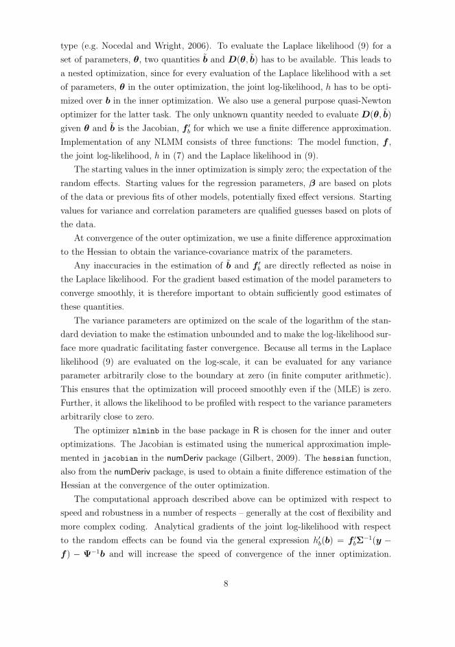
type (e.g. Nocedal and Wright, 2006). To evaluate the Laplace likelihood (9) for a
set of parameters, θ, two quantities b and D(θ, b) has to be available. This leads to
a nested optimization, since for every evaluation of the Laplace likelihood with a set
of parameters, θ in the outer optimization, the joint log-likelihood, h has to be opti-
mized over b in the inner optimization. We also use a general purpose quasi-Newton
optimizer for the latter task. The only unknown quantity needed to evaluate D(θ, b)
given θ and b is the Jacobian, f ′b for which we use a finite difference approximation.
Implementation of any NLMM consists of three functions: The model function, f ,
the joint log-likelihood, h in (7) and the Laplace likelihood in (9).
The starting values in the inner optimization is simply zero; the expectation of the
random effects. Starting values for the regression parameters, β are based on plots
of the data or previous fits of other models, potentially fixed effect versions. Starting
values for variance and correlation parameters are qualified guesses based on plots of
the data.
At convergence of the outer optimization, we use a finite difference approximation
to the Hessian to obtain the variance-covariance matrix of the parameters.
Any inaccuracies in the estimation of b and f ′b are directly reflected as noise in
the Laplace likelihood. For the gradient based estimation of the model parameters to
converge smoothly, it is therefore important to obtain sufficiently good estimates of
these quantities.
The variance parameters are optimized on the scale of the logarithm of the stan-
dard deviation to make the estimation unbounded and to make the log-likelihood sur-
face more quadratic facilitating faster convergence. Because all terms in the Laplace
likelihood (9) are evaluated on the log-scale, it can be evaluated for any variance
parameter arbitrarily close to the boundary at zero (in finite computer arithmetic).
This ensures that the optimization will proceed smoothly even if the (MLE) is zero.
Further, it allows the likelihood to be profiled with respect to the variance parameters
arbitrarily close to zero.
The optimizer nlminb in the base package in R is chosen for the inner and outer
optimizations. The Jacobian is estimated using the numerical approximation imple-
mented in jacobian in the numDeriv package (Gilbert, 2009). The hessian function,
also from the numDeriv package, is used to obtain a finite difference estimation of the
Hessian at the convergence of the outer optimization.
The computational approach described above can be optimized with respect to
speed and robustness in a number of respects – generally at the cost of flexibility and
more complex coding. Analytical gradients of the joint log-likelihood with respect
to the random effects can be found via the general expression h′b(b) = f ′
bΣ−1(y −
f ) − Ψ−1b and will increase the speed of convergence of the inner optimization.
8

The analytical Jacobian will also increase the speed of computation of the Hessian
approximation. A Gauss-Newton type estimation of the random effects can replace
the quasi-Newton optimization of the inner optimization using the gradient and the
Hessian, D from above. This often leads to further speed improvements. In models
with many random effects, the quasi-Newton estimation in the inner optimization
can benefit from memory-limited BFGS updates (Nocedal and Wright, 2006), and
the Gauss-Newton estimation can benefit from the use of sparse matrix methods (e.g.
Davis, 2006). Lastly, the residual variance can be profiled out of the likelihood thus
reducing the dimension of the outer optimization (Pinheiro and Bates, 1995).
3.2 Implementation in R
In this section we show how the models for the orange tree data presented in sec-
tion 1.1 can be estimated in a few lines of code with the computational approach for
the Laplace approximation described in section 3.1. First, we show how the simple
model (3) with a single scalar random effect is implemented. Subsequently we show
how this code can be altered in only a few places to fit model (4) with crossed ran-
dom effects, model (5) with a seasonal effect, and how the CAR process in (6) can be
allowed for in the latter models.
The model function, f for model (3) is defined as
> f <- function(beta, b)
(beta[1] + rep(b[1:5], each = 7))/
(1 + exp((beta[2] - time)/beta[3]))
The function returns a vector of the same length as the data with model predictions
based on the 3 fixed effects in beta, the 5 random effects in b and the 7 time points
in time. The joint negative log-likelihood based on (7) is defined as
> h <- function(b, beta, sigma, sigma.b)
-sum(dnorm(x = circumference, mean = f(beta, b),
sd = sigma, log = TRUE)) -
sum(dnorm(x = b[1:5], sd = sigma.b, log = TRUE))
using two vectorized calls to the univariate normal density function dnorm, because
the conditional distribution of the observations and the distribution of the random
effects are mutually independent normal. This is the negative joint log-likelihood,
because standard optimization algorithms by default minimize rather than maximize.
Based on the implementations of the model function and the joint log-likelihood,
the Laplace approximation to the marginal log-likelihood lLA(θ) is implemented as
> l.LA <- function(theta)
beta <- theta[1:3]
sigma <- exp(theta[4])
9

sigma.b <- exp(theta[5])
est <- nlminb(start = rep(0,5), objective = h, beta = beta,
sigma = sigma, sigma.b = sigma.b)
b <- est$par
h.b <- est$objective
Jac.f <- jacobian(func = f, x = b, beta = beta)
D <- crossprod(Jac.f)/sigma^2 + diag(1/sigma.b^2, 5)
h.b + 1/2 * log(det(D/(2 * pi))) .
where the parameters to be estimated are θ = (β, log σ, log σb). The call to nlminb
in l.LA performs the inner optimization and computes b, and the Hessian, D is
computed as in (8) based on the Jacobian, f ′b.
The maximum likelihood fit of model (3) is obtained by performing the outer
optimization with the call
> fit <- nlminb(theta0, l.LA)
where the starting values, θ0 are infered from Figure 1(a). The estimation converges in
a few seconds on a standard personal computer to the model fit presented in Table 1.
This concludes the estimation of model (3). Next, we show how this code can be
changed to estimate model (4) with crossed random effects. We mention all changes
to the code apart from updates to the parameter sets passed between functions and
similar trivialities. Only small changes to the code are required to estimate a model
that is not within reach with standard software for NLMMs. This illustrates the
power and flexibility of the proposed estimation scheme.
Model (4) has two crossed random components b1i and b2j for tree and time
and the full vector of random effects is thus b = [b11, ..., b15, b21, ..., b27]T . The
model function f is modified to include the 7 new random effects for sampling oc-
casion by adding the term rep(b[6:12], 5) to beta[1] + rep(b[1:5], each = 7).
To accommodate the additional random effects with standard deviation σb2 in the
joint log-likelihood, the function h is updated by adding -sum(dnorm(x = b[6:12],
sd = sigma.b2, log = TRUE)) to the existing code. The only change to the Laplace
likelihood, l.LA is in the adaption of the change in the covariance matrix for the ran-
dom effects, Ψ to the Hessian, D in (8); the term diag(1/sigma.b^2, 5) is replaced
by diag(c(rep(1/sigma.b^2, 5), rep(1/sigma.b2^2, 7))). Model (4) is estimated
similarly to model (3) and the optimization converges in a matter of seconds to the
results shown in Table 1.
While model (4) is a significant improvement to model (3), model (5) with a
seasonal effect might be more appropriate than model (4) with a random effect of
sampling occasion. To fit model (5), the only change to the previously defined func-
tions; f, h and l.LA for model (3) is the addition of the term beta[4] * season in
10

the exp-term in f. The estimate of model (5) is also shown in Table 1. Because the
likelihood of model (5) is considerably higher than that of model (4) at the same
expense of parameters and producing almost exactly the same predictions, we prefer
model (5).
The model fit for model (5) is shown in Figure 2(a). By comparing this to the fit
of model (3) in Figure 1(a), it appears that model (5) seems to capture the variation
between sampling occasions. This is also verified by a plot of residuals versus time
in Figure 2(b), where the residuals within sample occasions are now centered around
zero and smaller than in Figure 1(b). The plots for model (4) are very similar to
those in Figure 2 for model (5).
0 500 1000 1500
050
100
150
200
Days since 31 Dec 1968
Tru
nk c
ircum
fere
nce
(mm
)
Tree 1Tree 2Tree 3Tree 4Tree 5
(a) Plot of model fit.
Days since 31 Dec 1968
Res
idua
ls (
mm
)
−15
−10
−5
0
5
10
15
0 500 1000 1500
’70 ’71 ’72 ’73
(b) Residuals versus time.
Figure 2: Plots for model (5) for orange tree data.
In Figure 2(b), the residuals for each tree have been connected by lines to illustrate
that a positive auto-correlation is present. Only small changes to the estimation
scheme are required to accommodate any correlation or covariance structure in the
residuals. In the following we will describe how the CAR process in (6) for the within
tree residuals can be implemented and included in the estimation of the models (4)
and (5). We implement the covariance matrix, Σ in (6) as
> Sigma.CAR <- function(phi, sigma)
diff <- (time[1:7] - rep(time[1:7], each=7))
delta.t <- matrix(diff / (365 / 2), nrow = 7, ncol = 7)
P <- sigma^2 * exp( - phi * abs(delta.t))
kronecker( diag(5), P)
where delta.t is a matrix of time differences and P is cov(ǫi). To accommodate the
CAR process in the residuals in models (4) and (5), the model functions remain as
previously described and the joint log-likelihood is defined as
11

> h <- function(b, beta, sigma, sigma.b, sigma.b2, phi)
Sigma <- Sigma.CAR(phi, sigma)
resid <- circumference - f(beta, b)
0.5 * (log(det(2*pi*Sigma)) + crossprod(resid, solve(Sigma,
resid))) - sum(dnorm(x = b[1:5], sd = sigma.b, log=TRUE)) -
sum(dnorm(x = b[6:12], sd = sigma.b2, log=TRUE))
where the notable difference from previously is that the first part of h is now writ-
ten as the logarithm of a multivariate normal density using the full residual co-
variance matrix Sigma (in model (5) the last call to dnorm concerning σb2 is ex-
cluded). The term (y − µ)TΣ−1(y − µ) in the normal density function is com-
puted using crossprod(resid, solve(Sigma, resid)), since this is numerically more
stable and more efficient than computing the term directly as defined. The only
change to l.LA to accommodate (6) is in the computation of the Hessian, D, where
crossprod(Jac.f)/sig^2 is changed to crossprod(Jac.f, solve(Sigma, Jac.f)). To
make the estimation of the correlation parameter, φ in the CAR process (6) un-
bounded, it is optimized on the log-scale. The estimates of models (4) and (5) with
the CAR process (6) are shown in Table 1. For both models, the CAR process is a sig-
nificant improvement with p-values <0.001 based on likelihood ratio tests. For model
(5), the correlation over half a year, and therefore roughly between sampling occa-
sions, is ρ = 0.81, which is equivalent to the correlation coefficient in a discrete AR(1)
model, where account is taken of missing sampling occasions. This corresponds to the
strong auto-correlation seen in Figure 2(b) between successive sampling occasions.
4 Graphical Methods for Inference and Validation
In this section we illustrate a number of graphical methods that are useful for inference
and validation of a model fit. First, we discuss how to obtain the profile likelihood
and corresponding confidence intervals, next we discuss the use of pseudo likelihoods
for assessing convergence, and finally we discuss how the accuracy of the Laplace
approximation can be assessed when random effects enter nonlinearly in the model
function.
The profile likelihood is an inferential tool in its own right, and it can be used
to make likelihood based confidence intervals instead of having to rely on the Wald
approximation. For a scalar parameter θ, the profile likelihood is defined as L(θ) =
maxη L(θ,η), where η are nuisance parameters and θ = (θ,η). Our approach contains
a single loop over the parameter of interest with repeated optimization with respect
to the remaining nuisance parameters. The profile likelihood can be interpolated
by a spline (e.g. spline in R) to reduce the number of values of θ for which the
12
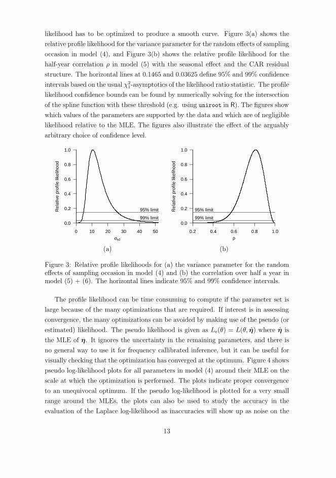
likelihood has to be optimized to produce a smooth curve. Figure 3(a) shows the
relative profile likelihood for the variance parameter for the random effects of sampling
occasion in model (4), and Figure 3(b) shows the relative profile likelihood for the
half-year correlation ρ in model (5) with the seasonal effect and the CAR residual
structure. The horizontal lines at 0.1465 and 0.03625 define 95% and 99% confidence
intervals based on the usual χ21-asymptotics of the likelihood ratio statistic. The profile
likelihood confidence bounds can be found by numerically solving for the intersection
of the spline function with these threshold (e.g. using uniroot in R). The figures show
which values of the parameters are supported by the data and which are of negligible
likelihood relative to the MLE. The figures also illustrate the effect of the arguably
arbitrary choice of confidence level.
0 10 20 30 40 50
0.0
0.2
0.4
0.6
0.8
1.0
Rel
ativ
e pr
ofile
like
lihoo
d
95% limit
99% limit
σb2
(a)
0.2 0.4 0.6 0.8 1.0
0.0
0.2
0.4
0.6
0.8
1.0
Rel
ativ
e pr
ofile
like
lihoo
d
ρ
95% limit
99% limit
(b)
Figure 3: Relative profile likelihoods for (a) the variance parameter for the randomeffects of sampling occasion in model (4) and (b) the correlation over half a year inmodel (5) + (6). The horizontal lines indicate 95% and 99% confidence intervals.
The profile likelihood can be time consuming to compute if the parameter set is
large because of the many optimizations that are required. If interest is in assessing
convergence, the many optimizations can be avoided by making use of the pseudo (or
estimated) likelihood. The pseudo likelihood is given as Le(θ) = L(θ, η) where η is
the MLE of η. It ignores the uncertainty in the remaining parameters, and there is
no general way to use it for frequency callibrated inference, but it can be useful for
visually checking that the optimization has converged at the optimum. Figure 4 shows
pseudo log-likelihood plots for all parameters in model (4) around their MLE on the
scale at which the optimization is performed. The plots indicate proper convergence
to an unequivocal optimum. If the pseudo log-likelihood is plotted for a very small
range around the MLEs, the plots can also be used to study the accuracy in the
evaluation of the Laplace log-likelihood as inaccuracies will show up as noise on the
13

curve. In this way it is found that the error of the log-likelihood surface is on the order
10−7 to 10−10 for the models we have considered. This is sufficient for the gradient
based estimation of model parameters to be both robust and efficient.
170 190 210−127
−126
−125
Asym650 750
xmid300 340 380
scal
1.5 1.7 1.9−127
−126
−125
log(sigma)3.0 3.4 3.8
log(sigma.b)1.8 2.2 2.6 3.0
log(sigma.b2)
Figure 4: Pseudo log-likelihood profiles for model (4).
The Laplace approximation is exact for all models estimated in Section 3, be-
cause the random effects enter linearly in the model functions. Sometimes however,
random effects enter nonlinearly and the Laplace likelihood (9) is an approximation
to the marginal likelihood (2), and it is of interest to substantiate how accurate the
approximation is. We may assess the accuracy of the approximation by graphical
means, and to illustrate this, we will use a model that was briefly mentioned in the
introduction
yij =β1 + b1i
1 + exp[−((tj − β2)/β3 + b2j)]+ ǫij (10)
where b2j enter additively on the logit-scale and thus nonlinearly in the model func-
tion. This model has a log-likelihood of -125.39 which is almost identical to that of
model (4), cf. Table 1. Because the two random components in (10) are crossed,
the integral defining the marginal likelihood (2) is 12-dimensional. We know that
the Laplace approximation is exact in the 5 directions corresponding to the linear
random effect, b1i. We can examine how good the Laplace approximation to the
12-dimensional integral is in the directions corresponding to the random effects that
appear nonlinearly in the model function. This is not a rigid assessment of the ac-
curacy of the entire integral, but intuitively we expect the total error to be small,
if the error is negligible in the directions corresponding to the random effects that
appear nonlinearly in the model function. Because the random effects in each ran-
dom component are independent by definition, and because each random effect in
one component only depends on the random effects in the other component indirectly
14

through the fixed parameters, the Hessian, D (and H) is very close to orthogonal.
Therefore, the error of the Laplace approximation will not be notably larger in the
directions that we are not examining. The integrand is given by the joint likelihood,
and we may plot this as a function of one of the random effects that enter nonlinearly
in the model function, while holding the fixed effects and the remaining random ef-
fects fixed at their estimates, θ and b. The approximating Gaussian curve illustrates
the Laplace approximation and is based on b and the appropriate diagonal entry of
D(θ, b). Figure 5 illustrates the joint likelihood (solid line) and the approximating
Gaussian curve (dashed line) for the random effects b24 (a) and b27 (b). We expect
there to be more information about the random effect b24 than about b27 due to the
structure of the logistic curve (b24 is at a sampling occasion, where the slope of the
logistic curve is large, and b27 is near the asymptotic circumference, where variations
has a smaller influence on the model function, cf. Figure 1(a)). This is reflected in
Figure 5 in two respects: 1) The curve is wider for b27 than for b24, 2) the curve for
b24 is better approximated by the Gaussian curve than the curve for b27.
−0.10 0.00 0.10 0.20
0.0e+00
5.0e−55
1.0e−54
1.5e−54
(a) b24
−0.4 −0.2 0.0 0.1 0.2
0.0e+00
5.0e−55
1.0e−54
1.5e−54
(b) b27
Figure 5: Joint likelihood (solid line) at the MLE for two random effects that enternonlinearly in the model function and the Gaussian approximation (dashed line).
Using a general integration function (integrate in base package in R), we evaluated
the integrals of the joint likelihoods in Figure 5 with sufficient precision and found
that the relative error of the Laplace approximation in these directions are 0.08% and
0.22%. The error in the directions corresponding to the remaining random effects
that enter non-linearly in the model (10) is of similar size, and we conclude that the
error of the Laplace approximation is negligible from a statistical perspective for this
model.
In model (10), D is an approximation to H due to the nonlinearity of the model
function in the random effects. At the parameter estimates the absolute error in
using D rather than H in the term − log |D/(2π)|/2 in the Laplace approximation
(9) is 0.0058 which is irrelevant from a statistical perspective and lends support to the
previous remark that the second-order term ignored in D is of negligible magnitude.
15

5 Comparison to Standard Software
The Laplace approximation gives the exact marginal likelihood for model (3) for
the orange data, because random effects enter linearly in the model function. The
model is an example of a simple NLMM with just one random component and can
be handled by all standard software. The model is used to compare the accuracy
of the R-based estimation scheme to SAS NLMIXED, NONMEM and nlme and the
results are shown in Table 2. Both SAS NLMIXED and NONMEM were used with
the Laplace approximation, and, as can be seen from the table, they both agree with
the implementation presented in this paper to all reported digits (NONMEM uses
an objective function missing a constant term log(2π)∑
ni (Wang, 2007), which has
been corrected for in the table). Also the parameter and std. err. estimates were
found to be very similar. The last row in Table 2 is nlme using Lindstrom and Bates’
(1990) alternating method, which is not exact for this model. The approximate log-
likelihood at the MLE deviates slightly from the others, which is also the case for the
parameter estimates.
Table 2: Values of the Log-likelihood for model (3) as reported by various software.l.LA in R -131.5718851SAS NLMIXED -131.57188NONMEM -131.5718nlme in nlme -131.5845
6 Discussion
The presented estimation scheme using the multivariate Laplace approximation offers
a very large flexibility in the specification of NLMMs at the cost of only a rather
limited amount of coding. It provides an option to fit models, assess convergence and
draw inference via profile likelihoods when standard software falls short. Especially
models with crossed random effects are not (at least easily) handled by any currently
available software package such as NONMEM, SAS NLMIXED, or nlme for R/S-
Plus. In this way the approach presented here fills a gap left by standard software
for NLMMs. The analysis of the orange tree data presented here shows that the
flexibility and ability to estimate, compare and draw inference from various models is
of substantial importance to the conclusions of the data analysis. The approximation
error of the Laplace approximation appears to be of only minor importance.
Several other methods for approximating the marginal likelihood of NLMMs than
that of Laplace have been proposed including Gauss Hermite quadrature (GHQ) (e.g.
16
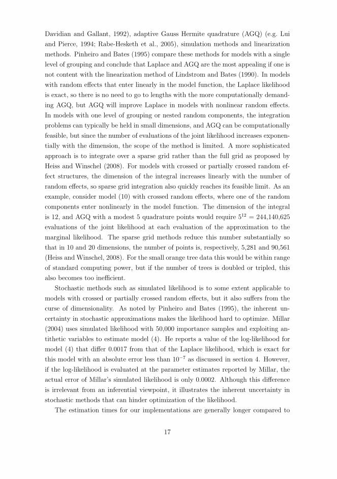
Davidian and Gallant, 1992), adaptive Gauss Hermite quadrature (AGQ) (e.g. Lui
and Pierce, 1994; Rabe-Hesketh et al., 2005), simulation methods and linearization
methods. Pinheiro and Bates (1995) compare these methods for models with a single
level of grouping and conclude that Laplace and AGQ are the most appealing if one is
not content with the linearization method of Lindstrom and Bates (1990). In models
with random effects that enter linearly in the model function, the Laplace likelihood
is exact, so there is no need to go to lengths with the more computationally demand-
ing AGQ, but AGQ will improve Laplace in models with nonlinear random effects.
In models with one level of grouping or nested random components, the integration
problems can typically be held in small dimensions, and AGQ can be computationally
feasible, but since the number of evaluations of the joint likelihood increases exponen-
tially with the dimension, the scope of the method is limited. A more sophisticated
approach is to integrate over a sparse grid rather than the full grid as proposed by
Heiss and Winschel (2008). For models with crossed or partially crossed random ef-
fect structures, the dimension of the integral increases linearly with the number of
random effects, so sparse grid integration also quickly reaches its feasible limit. As an
example, consider model (10) with crossed random effects, where one of the random
components enter nonlinearly in the model function. The dimension of the integral
is 12, and AGQ with a modest 5 quadrature points would require 512 = 244,140,625
evaluations of the joint likelihood at each evaluation of the approximation to the
marginal likelihood. The sparse grid methods reduce this number substantially so
that in 10 and 20 dimensions, the number of points is, respectively, 5,281 and 90,561
(Heiss and Winschel, 2008). For the small orange tree data this would be within range
of standard computing power, but if the number of trees is doubled or tripled, this
also becomes too inefficient.
Stochastic methods such as simulated likelihood is to some extent applicable to
models with crossed or partially crossed random effects, but it also suffers from the
curse of dimensionality. As noted by Pinheiro and Bates (1995), the inherent un-
certainty in stochastic approximations makes the likelihood hard to optimize. Millar
(2004) uses simulated likelihood with 50,000 importance samples and exploiting an-
tithetic variables to estimate model (4). He reports a value of the log-likelihood for
model (4) that differ 0.0017 from that of the Laplace likelihood, which is exact for
this model with an absolute error less than 10−7 as discussed in section 4. However,
if the log-likelihood is evaluated at the parameter estimates reported by Millar, the
actual error of Millar’s simulated likelihood is only 0.0002. Although this difference
is irrelevant from an inferential viewpoint, it illustrates the inherent uncertainty in
stochastic methods that can hinder optimization of the likelihood.
The estimation times for our implementations are generally longer compared to
17

those of standard software packages, when these are able to estimate the specified
models. The most complex model considered here is model (4) with the CAR structure
and it takes a few minutes to fit. The remaining models converges in a matter of a
few seconds directly to the MLE without any further effort. Larger data sets will
inevitably increase estimation times, but not necessarily the code complexity. In
some cases the optimizations of the computational approach mentioned in section 3.1
might be worth the effort.
In this paper we have illustrated the flexibility of estimation with the multivariate
Laplace approximation in the framework of NLMMs, but this method is applicable for
a much larger class of models. Essentially all mixed models, where the joint likelihood
is easily defined can be accommodated including the important generalized linear
mixed models; univariate as well as multivariate, and also the less common generalized
nonlinear mixed models. When the distribution of the observations is not Gaussian,
the Laplace approximation is naturally less accurate, but by the Bayesian central limit
theorem (Carlin and Louis, 2000), the joint likelihood tends to a normal curve when
the number of observations per random effect increase, so the Laplace approximation
can be expected to be fairly accurate when the information per random effect is not
small. In our experience the Laplace approximation is remarkably accurate for a wide
range of models, but further research is needed to address this topic formally.
Appendix
Table 3: Circumference in millimeters for 5 orange trees reported by Draper andSmith (1981, p. 524).
Tree Time (days since 31 Dec. 1968)
118S 484S 664A 1004A 1231S 1372A 1582S
1 30 58 87 115 120 142 1452 33 69 111 156 172 203 2033 30 51 75 108 115 139 1404 32 62 112 167 179 209 2145 30 49 81 125 142 174 177
A, S: Autumn, Spring
References
Barndorff-Nielsen, O. and D. R. Cox (1979). Edgeworth and saddle-point approximations
with statistical applications. Journal of the Royal Statistical Society, Series B 41, pp.
18

279–312.
Barndorff-Nielsen, O. E. and D. R. Cox (1989). Asymptotic Techniques for Use in Statistics.
London: Chapman & Hall.
Bates, D. M. and D. G. Watts (1980). Relative curvature measures of nonlinearity. Journal
of the Royal Statistical Society, B 42 (1), pp. 1–25.
Bates, D. M. and D. G. Watts (1988). Nonlinear Regression Analysis and Its Applications.
Wiley, New York.
Beal, S. L. and L. B. Sheiner (2004). NONMEM® Users Guide. NONMEM Project Group,
University of California, San Francisco.
Carlin, B. P. and T. A. Louis (2000). Bayes and Empirical Bayes Methods for Data Analysis
(2nd ed.). Chapman & Hall/CRC.
Davidian, M. and A. R. Gallant (1992). Smooth nonparametric maximum likelihood es-
timation for population pharmacokinetics, with application to quinidine. Journal of
Pharmacokinetics and Biopharmaceutics 20, pp. 529–556.
Davis, T. A. (2006). Direct Methods for Sparse Linear Systems. SIAM, Philadelphia.
Diggle, P. J., P. Heagerty, K.-Y. Liang, and S. L. Zeger (2002). Analysis of Longitudinal
Data (2nd ed.). Oxford university Press.
Draper, N. R. and H. Smith (1981). Applied Regression Analysis (2rd ed.). Wiley, New
York.
Gilbert, P. (2009). numDeriv: Accurate Numerical Derivatives. R package version 2009.2-1.
Heiss, F. and V. Winschel (2008). Likelihood approximation by numerical integration on
sparse grids. Journal of Econometrics 144, pp. 62–80.
Laird, N. M. and J. H. Ware (1982). Random effects models for longitudinal data. Biometrics
38, pp. 963–974.
Lindstrom, M. J. and D. M. Bates (1990). Nonlinear mixed effects models for repeated
measures data. Biometrics 46, pp. 673–687.
Lui, Q. and D. A. Pierce (1994). A note on gauss-hermite quadrature. Biometrika 81, pp.
624–629.
Millar, R. B. (2004). Simulated maximum likelihood applied to non-gaussian and nonlinear
mixed effects and state-space models. Australian & New Zealand Journal of Statistics
46, pp. 543–554.
19

Nocedal, J. and S. J. Wright (2006). Numerical optimization (2nd ed.). Springer.
Pinheiro, J., D. Bates, S. DebRoy, D. Sarkar, and the R Core team (2008). nlme: Linear
and Nonlinear Mixed Effects Models. R package version 3.1-90.
Pinheiro, J. C. and D. M. Bates (1995). Approximations to the nonlinear mixed-effects
model. Jounal of Computational and Graphical Statistics 4, pp. 12–35.
Pinheiro, J. C. and D. M. Bates (2000). Mixed-Effects Models in S and S-PLUS. Springer.
R Development Core Team (2008). R: A Language and Environment for Statistical Com-
puting. Vienna, Austria: R Foundation for Statistical Computing. ISBN 3-900051-07-0.
Rabe-Hesketh, S., A. Skrondal, and A. Pickles (2005). Maximum likelihood estimation of
limited and discrete dependent variable models with nested random effects. Journal of
Econometrics 128, pp. 301–323.
SAS Institute Inc. (2004). SAS/Stat 9.1 User’s Guide. Cary, NC: SAS Institute Inc.
Tierney, L. and J. B. Kadane (1986). Accurate approximations for posterior moments and
marginal densities. Journal of the American Statistical Association 81, pp. 82–86.
Vonesh, E. F. (1996). A note on the use of laplace’s approximation for nonlinear mixed-
effects models. Biometrika 83, pp. 447–52.
Wang, Y. (2007). Derivation of various NONMEM estimation methods. Journal of Phar-
macokinetics and Pharmacodynamics 34, pp. 575–593.
Wolfinger, R. D. (1999). Fitting nonlinear mixed models with the new
nlmixed procedure. In Proceedings of the Twenty-Fourth Annual SAS Users
Group International Conference, Number 287, SAS Institute Inc., Cary, NC.
http://ssc.utexas.edu/docs/sashelp/sugi/24/Stats/p287-24.pdf.
Wolfinger, R. D. and X. Lin (1997). Two taylor-series approximation methods for nonlinear
mixed models. Computational Statistics & Data Analysis 25, pp. 465–490.
20