Markets, Contracts, and Uncertainty: A Structural

Model of a Groundwater Economy

Xavier Gine and Hanan G. Jacoby∗

September 3, 2014

Abstract

Access to groundwater has been a key driver of agricultural productivity growth

and rural poverty reduction in south Asia. Yet, markets for groundwater are far from

perfectly competitive. We develop a contract-theoretical model of groundwater transac-

tions under payoff uncertainty, which arises from unpredictable fluctuations in ground-

water availability during the agricultural dry season. Our focus is on the tradeoff

between the ex-post inefficiency of seasonal contracts and the ex-ante inefficiency of

more flexible water-selling arrangements. We structurally estimate the model using

micro data on area irrigated under each transaction type combined with subjective

probability distributions of end-of-season borewell discharge collected from over 1,600

well-owners across four districts in southern India. We use the estimates to quantify

the contracting distortion and its impact on the development of groundwater markets.

∗Development Research Group, The World Bank, 1818 H St. NW, Washington DC, 20433. Gine:xgine@worldbank.org; Jacoby: hjacoby@worldbank.org. We owe a particular debt to K.P.C. Rao for hisefforts in managing the field work associated with this study, and to his survey team. We also thank MarkGersovitz for extraordinarily useful comments on an earlier draft, as well as seminar participants and severaldiscussants for their ideas and suggestions. Financial support for this project was provided by the ResearchCommittee of the World Bank. Views expressed in this paper are those of the authors, and do not necessarilyreflect the opinions of the World Bank, its executive directors, or the countries they represent.

1 Introduction

A central theme in the economics of organization is that long-term contracts protect invest-

ments specific to a trading relationship. The early transactions costs literature (Williamson,

1971; Klein et al., 1978) recognized not only these benefits of long-term contracts but also

the costs; in an uncertain environment, contractual rigidity inevitably leads to resource mis-

allocation, a distortion obviated by ex-post or spot contracting. Empirical research within

this tradition thus asked two complementary questions: Does the duration of long-term con-

tracts depend on the degree of asset specificity (Joskow, 1987)? And, are long-term contracts

structured so as to adapt to changing economic conditions (e.g., Goldberg and Ericson, 1987;

Masten and Crocker, 1985; Crocker and Masten, 1988)? But, the choice of long-term over

spot contract, and whether it too is driven by this fundamental tradeoff between ex-ante and

ex-post inefficiency, has not been rigorously investigated.1

To fill this lacuna, we consider an environment–agricultural production in southern India–

characterized by substantial upfront investment as well as by uncertainty regarding a critical

input into subsequent production stages: groundwater extracted from private borewells, the

exclusive source of dry-season irrigation. In light of the link between access to groundwater,

or lack thereof, and rural poverty in South Asia (Shah, 2007; Sekhri, 2013), there is a growing

economics literature on groundwater markets (e.g., Anderson, 2011; Banerji et al., 2012;

Foster and Sekhri, 2008; Jacoby et al., 2004). Since water is extremely costly to transport,

these markets tend to be highly spatially fragmented and, hence, inherently uncompetitive.

In our setting, bilateral transactions between well-owners and neighboring farmers take one

of two forms: spot contracts, in which groundwater is sold on a per-irrigation basis, and

long-term (i.e., seasonal) contracts, which specify price and area irrigated over an entire

crop cycle ex-ante.

We develop a model in which spot contracts are fully state contingent and thus ex-post

efficient, but, due to the classic holdup problem, ex-ante inefficient. In particular, planting

incentives of water-buyers are distorted. Long-term contracts, by contrast, are assumed

to deter holdup,2 but lead to ex-post inefficiency insofar as groundwater is misallocated

1Lafontaine and Slade (2012) provide a thorough review of empirical research on inter-firm contractingfrom various theoretical perspectives. A strand of the literature does consider the choice between long-termcontracts and spot markets (e.g., Carlton, 1979; Polinsky, 1987; Hubbard and Weiner, 1992). However, inthese models, there is no relationship-specific investment; firms incur the transactions costs of long-termcontracts to insure against cash-flow variability.

2On this point, we appeal to the recent insight of Hart and Moore (2008) that contracts act as referencepoints, establishing what each party in the transaction is entitled to. Opportunism thus leads to deadweightlosses. In the earlier property rights theory of the firm associated with Grossman and Hart (1986) and Hart

1

across farms once the state of nature is revealed. Our model yields the sharp prediction

that as groundwater supply uncertainty increases, long-term contracts become unattractive

relative to spot arrangements. In addition, higher uncertainty reduces the overall extent of

groundwater markets.

A key contribution of this paper lies in quantifying these contracting distortions, as well

as their impacts, using a structural econometric model. A rather unique feature of a ground-

water economy that allows us to do this is that buyers and sellers are both agricultural

producers, cultivating side-by-side with the same technology, the total returns to which are

(to a first approximation) proportional to area irrigated. Gagnepain et al. (2013) is another

rare example of structural estimation and quantitative welfare analysis within the empirical

contracts literature. While their analysis of the tradeoff between ex-post renegotiation and

ex-ante incentives in the context of French public-sector contracts bears a superficial resem-

blance to ours, contractual choice is driven in their case by asymmetric information rather

than, in our case, by what Hart (2009) terms payoff uncertainty. Moreover, in the setting

we consider, agents have the option not to contract or trade at all (and many do not), which

allows us to investigate how payoff uncertainty affects overall market activity.

Our model of agricultural production under stochastic groundwater supply accounts for

the choice between seasonal contracts and per-irrigation sales, for water transfers through

leasing, and (crucially) for the areas irrigated under each such arrangement. We have data

collected from a large sample of borewell owners across six districts of Andhra Pradesh and

Telangana states in southern India. Our specially-designed groundwater markets survey

takes particular care to elicit from each respondent a subjective probability distribution of

their borewell’s discharge near the end of the season conditional on its initial discharge. The

structural parameters of the model are identified principally off of variation across borewells

in this conditional probability distribution.3

To assess external validity of the structural model, we retain a nonrandom holdout sam-

ple consisting of two districts; borewells from the remaining four districts constitute the

estimation sample on which we fit the model. Thus, we follow Keane and Wolpin (2007)

who argue for choosing “a [holdout] sample that differs significantly from the estimation

and Moore (1990), renegotiation is efficient so that holdup is virtually inevitable (Hart, 1995). As a result,there is no functional difference between contracts agreed upon ex-ante and those agreed upon ex-post. Fehret al. (2011) and Hoppe and Schmitz (2011) corroborate the reference-point idea experimentally.

3While several recent papers incorporate subjective probabilities into structural econometric models (see,e.g., Delvande, 2008; Mahajan et al., 2011; Mahajan and Tarozzi, 2012), ours is the first such application inthe contracts literature. Delavande et al. (2010) discuss issues in collecting subjective expectations data indeveloping countries.

2

sample along the policy dimension that the model is meant to forecast (p. 1352).” The

analogue, in our setting, to a policy regime “well outside the support of the data” is the

large difference in levels of groundwater supply uncertainty between borewells in the four es-

timation sample districts (low uncertainty) as compared to the two holdout sample districts

(high uncertainty).

Using the structural parameter estimates, we perform two counterfactual exercises. In

the first, we ask how much of the stark regional difference in contractual arrangements and

groundwater market development can be attributed to geographic variation in uncertainty.

In the second, we use the device of a hypothetical land consolidation program to estimate the

magnitude of the distortions induced by groundwater uncertainty. If all plots surrounding

a given borewell were owned by the same individual (i.e., consolidated), then contracting

distortions would be irrelevant.

The next section of the paper lays out the formal theoretical arguments. Section 3

describes our survey data and the groundwater economy of southern India in greater detail.

Section 4 adapts the theoretical model for the purposes of structural estimation and derives

the likelihood function. Estimation results and counterfactual simulations are reported in

Section 5. Section 6 concludes.

2 Theory

2.1 Preliminaries

We begin by briefly enumerating our assumptions, leaving the more extended justifications

for section 3.

A.1) Fragmentation: Agricultural production occurs on discrete plots of land of area a,

each owned by a distinct individual.

This presupposes that the outright purchase of neighboring plots is generally infeasible,

perhaps due to mortgage finance constraints. At any rate, (A.1) is backed by data, since, as

we will see, a large majority of plots are inherited.

A.2) Borewells and groundwater: A reference plot has a borewell drawing a stochastic

quantity of groundwater w over the growing season, where w has p.d.f. ψ(w) on

support [wL, wH ]. Groundwater is the sole irrigation source.

3

Property rights to groundwater are not clearly delineated in India, so there is no legal limit

to withdrawals. Because electricity is provided free at the margin, farmers run their pumps

for the maximum number of hours that power is available on any given day. Aside from this

constraint, w depends on the capacity of the well (pipe-width), availability of groundwater

in the aquifer, and the local hydrogeology.

A.3) Technology: The common crop output production function, y = F (l, w, x), depends on

three inputs: land l, seed x, and water w, with land and seed used in fixed proportions.

For any level of x, y/l = f(w/l) ≡ f(ω), where ω is irrigation intensity and the intensive

production function, f , is increasing, concave, with f(0) = 0.4

Given (A.3), we may write net revenue as lf(ω) − c, where c is the cost of the required

seed per acre cultivated.

A.4) Risk preferences: Farmers are risk neutral.

We defer a discussion of the role of risk preferences to the next section, only noting here that

risk-neutrality is a core assumption of the transactions cost literature.

A.5) Adjacent land: A well-owner is not limited in the area of adjacent land that his borewell

can irrigate.

In invoking (A.5), we abstract from any demand-side constraints such as may arise when

most or all adjacent landowners also have their own borewells. While this assumption vastly

simplifies the theoretical analysis, it is is clearly unrealistic and, for this reason, it will be

relaxed in the empirical implementation.

Consider, first, a well-owner’s choice of area cultivated (irrigated) when his own plot size

is not a constraint. Let `S = arg max l Ef(w/l)− c and define the marginal return as

Definition 1 g(ω) = f(ω)− ωf ′(ω).

The necessary condition for optimal planting

Eg(ω) = c (1)

4Constant returns to scale is both technically convenient and empirically sensible. Diminishing returnsis unlikely to set in over the range of cultivated areas that we are considering. Moreover, under diminishingreturns, well-owners might simultaneously leave their own plot partially fallow while selling water to aneighboring plot, a scenario which is virtually never observed in practice.

4

equates the expected marginal return to the marginal cost of cultivation.

Now, letting r index mean preserving increases in groundwater supply uncertainty, we

have

Proposition 1 (Precautionary planting) If g is strictly concave, then ∂`s/∂r < 0.5

In other words, well-owners may evince a precautionary motive analogous to that in the

savings literature (e.g., Kimball, 1990), in this case limiting their exposure to increases in

supply uncertainty by committing less area to irrigate.

The surplus generated by a borewell under unconstrained self-cultivation is

Definition 2 VS = `SE [f(w/`S)− c] .

In case `S > a, we may think of VS as the surplus derived by the well-owner if he could

sell groundwater in a competitive spot market.6 As mentioned, however, groundwater trans-

actions do not resemble this competitive, arm’s-length, ideal. In what follows, we consider

bilateral contracting between well-owner and buyer. Our approach is to model only contracts

observed empirically, not hypothetical contracts that may nevertheless be globally optimal.7

2.2 Long-term contracts

The canonical long-term contract in our setting commits the well-owner to irrigate a buyer’s

field, or some portion thereof, for the whole season at a pre-determined price. Following

Hart and Moore (2008), we think of such (ex-ante) contracts as establishing entitlements.

Ex-post renegotiation of the terms, or hold-up, will therefore lead to deadweight losses due

to aggrievement by one or both parties.8 To bring the tradeoff between ex-ante and ex-

post inefficiency into stark relief, we assume that these deadweight losses make hold-up

5Proof: Follows directly from Theorem 1 of Diamond and Stiglitz (1974).6 To see why, let subscripts b and s denote water-buyer and seller, respectively. Further, let p be the

spot price and `b the buyer’s cultivated area such that `S = a+ `b. It is easy to see that f ′(ωb) = f ′(ωs) =p which implies that ωb = ωs. Thus, VS = E [a(f(ωs)− c) + pωb`b] = E [a(f(ωs)− c) + f ′(ωb)ωb`b] =E [a(f(ωs)− c) + `b(f(ωb)− c)] = E [(a+ `b)(f(ωs)− c)] , where the penultimate expression follows fromEg(ωb) = c, the necessary condition for the buyer’s optimal area cultivated.

7For example, a long-term contract indexed to the state of nature may be first-best (see, e.g., Hart, 2009),but such arrangements are not observed in practice.

8More precisely, this literature assumes that there are noncontractible actions that either party can takeex-post to add value to the transaction. As long as a party feels he is getting what he is entitled to inthe contract, he will undertake such helpful actions, but if he feels shortchanged he will withhold them,generating a loss in surplus. In the words of Hart (2009): “Although our theory is static, it incorporatessomething akin to the notion of trust or good will; this is what is destroyed if hold-up occurs.” (p. 270).

5

prohibitively costly. Thus, the seasonal contract has two salient features: (1) by serving as

reference point in, and hence as a deterrent to, renegotiation, it protects relationship-specific

investment (in our context, planting inputs); and (2) water allocations under the contract

are unresponsive to the state of the world.

Let τ denote the total transfer of groundwater at per unit price p to irrigate a field of

size l. The optimal simple (i.e. single-price) contract solves

maxp,l

a

Ef(

w − τa

)− c

+ pτ s.t.

PC : lf(τ

l)− c

− pτ ≥ 0 (2)

IC : τ = arg maxτ∈[0,wL)

lf(τ

l)− c

− pτ

The first term in the well-owner’s objective function (top line) is the expected revenue from

crop production on his own plot net of cultivation costs, which is diminished when he sells

water to a neighbor; the second term is his total revenue from the sale. The participation

constraint (PC) stipulates that the crop revenue of the buyer net of both cultivation and

water costs cannot be negative. Finally, the incentive constraint (IC) says that the transfer

is maximizing the buyer’s net revenue, subject to the constraint that the promised amount

cannot exceed the available supply of water in the lowest state of the world, wL. Note that

expectations are dropped in both the PC and IC because, under the contract, l and τ are

fixed ex-ante. Thus, the seasonal contract offers an assured supply of irrigation to the buyer;

the direct cost of production variability is borne fully by the seller on his plot.

Given a binding PC, the necessary conditions for the optimal contract are as follows:

Ef ′(w − τa

)= p

g(τl

)= c (3)

f ′(τl

)= p,

the solution to which is the water transfer-area pair (τC , `C). Divergence of supply and

demand for irrigation ex-post creates a distortion. Since (3) implies Ef ′(w−τCa

)= f ′

(τC`C

),

it is not true, in general, that f ′(w−τCa

) = f ′( τC`C

) ∀ w, which would obtain if p and τ were

state-contingent, as in a competitive spot market (see fn. 6). It follows as a corollary that

6

the distortion vanishes as ψ becomes degenerate, in which case g( τC`C

) = g( w`C+a

) = c = g( w`S

)

which implies that `C = `S − a. Thus, in the absence of uncertainty, the amount of land

irrigated and the economic surplus generated by the borewell would be the same under the

seasonal contract as under a competitive spot market; i.e., the long-term contract would

achieve the first-best.

2.3 Spot contracts

Groundwater may also be sold on a per-irrigation basis. Once the season is underway,

however, commitments have been made. The potential seller has retained (i.e., refrained

from contracting out) the rights to some excess water from his well during the season whereas

the potential buyer has planted a crop in an adjacent plot.9 Since each party has some degree

of bargaining power, we use a Nash bargaining framework.

To be clear, in a per-irrigation arrangement, there is a self-enforcing agreement to trade

during the course of the season, even though the terms of these trades are not necessarily

delineated ex-ante. Indeed, side-payments may be made (or favors rendered) to secure an

exclusive trading relationship. We assume that any negotiations at this stage are efficient;

in other words, the parties will leave no money on the table.10

Returning to the ex-post stage, let τ be the amount of water already transferred to the

buyer and suppose that buyer and seller negotiate the price p of incremental transfer ∆.

The buyer’s net payoff from consummating the trade is given by u = lf((τ + ∆)/l) − p∆,

whereas that of the seller is v = af((w− τ −∆)/a) +p∆. The no-trade payoffs are given by

u = lf(τ /l) and v = af((w− τ)/a), respectively. The absence of c in these payoff functions

reflects the fact that all cultivation costs have already been incurred.

Given Nash bargaining, p∗ = arg max(u− u)η(v−v)1−η, where η is the buyer’s bargaining

weight. Therefore, p∗ solves

9An early descriptive study of groundwater markets in a Tamil Nadu village captures the buyer’s predica-ment: “A particularly potent source of control which a water seller can exercise over a water purchaser isthat the former is in a position to stop supplying water to the latter at a crucial stage of crop growth, onalleged grounds of his pumpset being in a broken down state, or some such similar, transparently flimsyexcuse. A cessation of the provision of water after an initial supply lasting for a month or forty-five dayscould expose the water purchaser, who by then would have invested substantially in raising the crop, to thedanger of heavy losses. Neither is the purchaser free to turn to an alternative supplier of water: a customarypractice in force in the village ensures that a water seller may supply water only to owners of contiguousplots...” (Janakarajan, 1993, p. 71)

10We also abstract from any reallocation of property rights between the parties at this stage that redis-tributes ex-post bargaining power a la Grossman and Hart (1986). Later, in the empirical model, we allowfor one form of vertical integration: the well-owner can lease an adjacent plot without a well of its own,although this too is costly.

7

η(v − v)− (1− η)(u− u) = 0

ηa

[f(w−τ−∆

a)− f(w−τ

a)

∆

]− (1− η)l

[f( τ+∆

l)− f( τ

l)

∆

]+ p = 0 (4)

−ηf ′(w − τa

)− (1− η)f ′

(τl

)+ p = 0

where the last line takes the limit of the second line as ∆→ 0. Thus, we obtain the standard

surplus-splitting rule

p∗(τ) = (1− η)f ′(τ

l

)+ ηf ′

(w − τa

). (5)

Furthermore, once f ′( τl)−p∗(τ) = η

[f ′( τ

l)− f ′(w−τ

a)]

= 0, the buyer’s demand for irrigation

is sated. Thus, the total transfer τ must satisfy f ′( τl) = f ′(w−τ

a), which is the condition for

an ex-post efficient allocation of groundwater conditional on area cultivated.

Now consider the buyer’s ex-ante problem of choosing area cultivated to maximize ex-

pected returns given price function p∗ and the total transfer τ . In particular,

`P = arg maxlE

lf(τl

)−∫ τ

0

p∗(t)dt

− cl. (6)

Observe that the per unit price of water is now state-dependent and, in particular, is no

longer constant as in the seasonal contract; each small increment of irrigation now has a

different cost. From (5),∫ τ

0p∗(t)dt = (1 − η)lf( τ

l) + ηa

[f(w−τ

a)− f(w

a)], so only the first

term on the right-hand side depends on l. The necessary condition for the buyer’s cultivation

choice is, therefore, simply

ηEg(τ/l) = c. (7)

Comparing equations (7) and (1), we see that they differ by the factor η. Surplus extraction

on the part of the water seller effectively taxes the marginal benefits of cultivation, with the

tax rate decreasing in the buyer’s bargaining power; efficiency is attained only if η = 1.

To summarize, spot contracts lead to an ex-post efficient allocation but distort ex-ante

incentives. The latter inefficiency is due to the hold-up problem first formalized by Grout

(1984); the buyer under-invests (indeed, `P < `S − a) in anticipation of ex-post rent appro-

priation.

8

2.4 Characterizing the tradeoff

We have already seen that the distortion induced by the long-term contract disappears when

groundwater supply becomes perfectly certain, whereas the distortion induced by the spot

contract does not. Next, we establish a general result about the dominance of long-term

over spot contracts in our environment.

Recall that increases in r correspond to mean preserving increases in uncertainty, with

r = 0 indicating perfect certainty. Let Vj(r) be the surplus derived from contract of type

j = C,P ,11 and note that VP (r, η) also depends on the bargaining weight η.

Proposition 2 (Dominance) If g is strictly concave and τC(0) < wL,12 then (a) for some

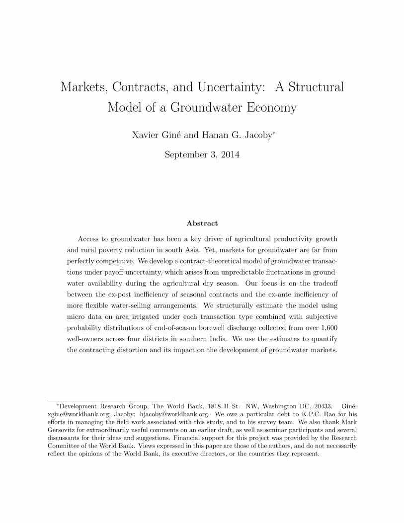
η, ∃ a unique r∗(η) such that VC(r∗) = VP (r∗, η); (b) [VC(r)− VP (r, η)] (r∗ − r) > 0.13

Simply put, under the conditions of proposition 2, there can be a level of uncertainty at

which the parties are indifferent between seasonal and per irrigation arrangements. If so,

then the seasonal contract must dominate at low levels of uncertainty and per-irrigation sales

at high levels of uncertainty.

Figure 1 illustrates the intuition underlying proposition 2, showing how the economic sur-

plus generated by a borewell varies with uncertainty level r under alternative water transfer

arrangements. Regardless of arrangement, surplus always decreases with r (see Appendix).

In the case of autarky (A), in which the borewell irrigates exactly plot area a, surplus is

VA = aE [f(w/a)− c] . VA must lie strictly below first-best surplus VS except at r = rS; at

this level of uncertainty, `S = a and autarky is the optimal unconstrained choice. When the

borewell owner sells water under a seasonal contract, surplus VC is also less than first-best

(except under perfect certainty), coinciding with VA at some positive level of uncertainty

rC < rS. Note that VC declines relatively rapidly with r because higher uncertainty operates

upon two margins under a seasonal contract: It leads to greater ex-post misallocation of

11For the seasonal contract, surplus is given by the private returns to the well-owner; since the PC isbinding, the water-seller gets all the surplus. By contrast, in the per-irrigation case, we must considerthe joint surplus of well-owner and water-buyer. It might be argued that the choice of per-irrigation overalternative arrangements should be governed by the water seller’s private returns as well. This, however,runs counter to our assumption that all ex-ante negotiations are efficient. In other words, situations inwhich the per irrigation arrangement yields the highest joint surplus but fails to maximize the well-owner’sprivate return would be resolved through side-payments.

12In words, this latter condition states that the water transfer under perfect certainty is less than totalwater available in the worst state of the world. Otherwise, VC has a discontinuity at r = 0; i.e., at r = ε, theoptimal transfer must be discretely less than τC(0). In this case, r∗(η) still exists for some η but it is notnecessarily unique. Part (b) of the proposition continues to hold, however, with respect to the largest r∗.

13Proof: See Appendix.

9

groundwater across plots as well as to a contraction of overall area irrigated by the borewell

(precautionary planting). Only the latter effect is operative under the per-irrigation arrange-

ment. In this case, surplus VP approaches VS as η approaches one. Moreover, at some low

level of bargaining power η = η, `P = 0 and VP coincides with VA. So, for some range of

η ∈ (η, 1), VP and VC must cross. Given such a crossing (at r∗), VP coincides with VA at

a level of uncertainty rP between rC and rS. This shows that the spot contract can only

dominate the long-term contract when uncertainty is high.

3 Data and Background

Our data come from a randomly selected survey of 2,423 borewell owners undertaken in six

districts of Andhra Pradesh (AP) and Telangana (until 2014, also part of AP) in 2012-13.

The districts were selected to cover a broad range of groundwater availability, conditions for

which generally improve as one moves from the relatively arid interior of the state toward the

lusher coast. Drought-prone Anantapur and Mahbubnagar districts were originally selected

as part of a weather-index insurance experiment (Cole et al., 2013); all 774 borewell owners

were followed up from that study’s 2010 household survey. Guntur and Kadapa districts,

which fall in the intermediate range of rainfall scarcity, and the water-abundant coastal

districts of East and West Godavari, each contribute around 400 borewell owners to our

sample.14

The 1,649 borewells in Guntur, Kadapa, East and West Godavari form our estimation

sample, whereas the 774 borewells in more arid Anantapur and Mahabubnagar districts

constitute a holdout sample that we use for model validation and counterfactual analysis.

3.1 Recharge and uncertainty

As in much of India, farmers in AP rely almost exclusively on groundwater during the rabi

(winter or dry) season, when rainfall is minimal and surface irrigation typically unavailable.

Indeed, the last two decades have seen an explosion of borewell investment as the cost of

drilling and of submersible electric pumpsets have fallen.15 Despite alarm about groundwater

overexploitation in India more broadly (e.g., New York Times, 2006; Economist, 2009),

14A total of 144 villages were covered (21-25 per district) in the survey. Our sample is broadly represen-tative of areas with sufficient groundwater for rabi cultivation and where groundwater is the sole source ofirrigation during that season (villages in canal command areas were avoided).

15Appendix figure A.1 documents the rising importance of borewell irrigation in all of India, in AP as awhole (prior to the 2014 partition), and in the six districts of our survey. See also World Bank (2005).

10

water-tables across AP do not exhibit much downward trend; rather, the time-series is

dominated by inter-annual variability (Appendix figure A.2). This is explained by the limited

storage capacity of the shallow hard rock aquifers that characterize the region. Most of

the recharge from monsoon rains occurring over the summer months is depleted through

groundwater extraction in the ensuing rabi season. In contrast to the hydrogeology of much

of North India, there are no deep groundwater reserves to mine (see Fishman et al., 2011).16

This annual cycle of aquifer replenishment and draw-down throughout AP is central to

our analysis of groundwater markets. Although farmers can observe monsoon rainfall along

with their own borewell’s discharge prior to rabi planting, they cannot perfectly forecast

groundwater availability over the entire season. To measure the degree of uncertainty, as

part of the borewell owner’s survey we fielded a well-flow expectations module, which was

structured as follows: First, we asked owners to assess the probability distribution of flow

on a typical day at the start of (any) rabi season, the metric for discharge being fullness of

the outlet pipe (i.e., full, 34

full, 12

full, 14

full, empty). Next, using the same format, we asked

about the probability distribution of end-of-season flow conditional on the most probable

start-of-season flow. Thus, the question was designed to elicit residual uncertainty about

groundwater availability.

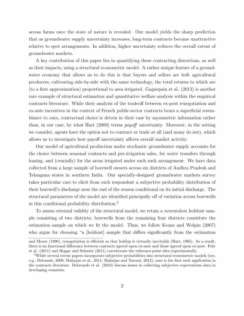
Figure 2 shows the distributions of groundwater uncertainty (well-specific coefficients

of variation of end-of-season flow) in both the estimation and holdout samples. The first

thing to notice is that virtually no borewell owner (except five in the estimation sample)

reports having a perfectly certain supply of groundwater. Secondly, the difference across

samples is striking; uncertainty is much higher in the holdout districts of Anantapur and

Mahabubnagar where aquifer recharge is relatively meager. One goal of the empirical work

below is to investigate whether this difference in uncertainty levels can account for the

similarly dramatic divergence in groundwater market activity across regions.

3.2 Land fragmentation, fixed costs, and groundwater markets

A second crucial element of our analysis is land fragmentation coupled with the high fixed cost

of borewell installation, on the order of US$1000 (excluding the pump-set). Fragmentation

is driven by the pervasive inheritance norm dictating equal division of land among sons and

the prohibitive transaction costs entailed in consolidating spatially dispersed plots through

16Shah (2009) emphasizes the role of different aquifer types in shaping groundwater governance arrange-ments in South Asia.

11

the land market.17 In our data, nearly 80 percent of plots were acquired through inheritance.

Land fragmentation would be irrelevant, of course, were groundwater markets frictionless.

If so, borewells would be just as likely on small plots as on large plots; the owner of a small

plot could simply sell any excess groundwater to a neighbor. Obversely, small plots would be

just as likely cultivated in the dry season as large plots; any plot owner without a borewell

of his own could purchase groundwater from that of a neighbor. Neither implication of

frictionless groundwater markets, however, is consistent with our data.

Our survey covers around 9600 plots, each of which either has a borewell itself or is

adjacent to a plot that does and, thus, could in principle receive a transfer of groundwater.

Figure 3 shows that borewells are actually much less likely on small plots than on large ones.

One might think that a random allocation of borewells across space could generate such a

pattern mechanically; larger plots would be more likely to have borewells insofar as they

constitute the majority of farmland area. But this ignores the fact that well placement is

determined by individual decision-makers at the plot-level. If there is an equal probability

of successfully finding groundwater regardless of where one drills for it and each plot-owner

makes the same number of drilling attempts, then the likelihood of observing a borewell

should be equal across plots, regardless of size.

To be sure, owners of small plots may also be less wealthy and thus unable to afford

multiple drilling attempts, or any attempts at all for that matter (see, e.g., Fafchamps and

Pender, 1996). To control for wealth, we focus only on the subset of plots whose owner has

at least one other plot; otherwise, plot area and total owned area are perfectly correlated.

We then partial out the effect of wealth (as proxied by total landholdings) using dummies

for each of the deciles of total landownership. The resulting figure 4 continues to show an

increasing borewell probability as plot size increases. Finally, figure 5 shows that small plots

are much more likely to be left fallow in the dry season than large plots. Taken together,

this evidence indicates frictions in groundwater markets.

3.3 Adjacency approach

To capture transfers of groundwater, which typically occur between adjacent plots so as to

minimize conveyance losses,18 we departed from the usual household-based sampling strategy.

17Appendix figure A.3 illustrates the increasing fragmentation in India, and in AP, as seen through therising proportion of marginal farms (those with operational landholdings of less than 1 hectare).

18Most irrigation water is transfered through unlined field channels with high seepage rates. While oursurvey also picked up a number of transfers to non-adjacent plots using PVC pipe, usually these casesinvolved sharing of groundwater between well co-owners or between multiple plots of the same owner.

12

Instead, each of the 2307 randomly chosen respondents (borewell owners) was also asked to

report on all the plots adjacent to the one containing the reference borewell,19 including

characteristics of the landowner, details on how the plot was irrigated during the rabi, if

not left fallow, and on the transfer arrangement if one occurred. This adjacency approach

provides information about not only the transfers that did happen but also about those that

could have happened but did not.

The number of plots adjacent to a reference borewell varies from 1 to 7, with a mode of 3.

Table 1 provides descriptive statistics on these plots, showing that in the estimation sample

42% are irrigated in whole or in part by the reference borewell. This figure falls to just 15%

of adjacent plots in the holdout sample, even though the proportion owned by brothers, who

are more likely to be co-owners of the reference borewell,20 is substantially higher in the

holdout sample. A similarly wide disparity exists in the percentages of plots accessing other

borewells, which may or may not be in the adjacency. Thus, transfers of groundwater, and

especially sales, are comparatively limited in the two holdout districts and commensurate

with this is a much higher fraction of fallow plots in rabi season.

In figure 6, we pool the two samples and aggregate plot-specific data to the adjacency

level. The top curve shows how borewell density in the adjacency–the average of the plot-level

borewell indicator used in figure 3 weighted by the plot’s area share in the adjacency–varies

with average plot size. Mirroring figure 3 at the adjacency level, it shows that borewell

development is less intensive on highly fragmented land. The bottom curve refers to the

proportion of plots in the adjacency receiving any groundwater transfer from the reference

well (aside from transfers between its co-owners). The frequency of such transactions falls

with average plot size in the adjacency.21 So borewell density and groundwater market

activity are substitutes, both driven by the degree of local land fragmentation.

3.4 Precautionary planting and risk aversion

Proposition 1 asserts that uncertainty in groundwater availability interacts with the irre-

versibility of the planting investment in an important way. However, the empirical impli-

cations of this interaction–in particular, whether there is indeed a precautionary planting

19There are 114 cases of the reference plot having a second borewell and 2 cases of it having a thirdborewell, which gives a total of 2423 reference wells.

20In constructing the data set for the structural estimation, we merge the plots of all co-owners of thereference borewell found in the adjacency.

21Each of the local polynomial fits in the figure retain practically identical shapes after adjusting outreference plot/well characteristics (plot area, area-squared, and outlet pipe diameter).

13

motive–hinges on the properties of g, the marginal return to planting, which is not di-

rectly observable. To motivate our functional form assumptions, therefore, we now present

a reduced-form analysis of planting decisions.

Crops grown during Rabi season in AP fall into two broad categories: wet crops (in

our six districts, principally paddy, banana, sugarcane, and mulberry) and irrigated-dry or

ID crops (e.g., groundnut, maize, cotton, chillies), distinguished by the much greater water

requirements of the former. Since a field that, planted to ID crops, would take 3 days to

irrigate, would take a week to irrigate under wet crops, we use the equivalence 1 acre wet =73

acre ID to compute total area irrigated by a borewell.22

We investigate the effect of uncertainty on planting decisions using both subjective and

objective outcome measures. The subjective outcome Y si for borewell i is derived from a

question in our survey asking each owner how many acres (wet and/or ID) would have been

irrigated with his borewell “if at the start of the rabi you knew for certain what the flow

during the rest of the season was going to be.”23 Thus,

Y si = log(actual irrigated area)− log(irrigated area under certainty).

In our full sample of 2, 423 borewells (i.e., estimation + holdout samples), the average Ys

is -0.280 (median is -0.231), indicating a (perceived) reduction in irrigated area due to un-

certainty on the order of 25%. To see how such precautionary planting behavior varies with

groundwater uncertainty, we report in panel (a) of Table 2 a regression of Y si on the log(CVi)

of end-of-season flow (see figure 2), as well as the log of outlet pipe-width (to control for

borewell capacity). The negative coefficient on log(CVi) in column 1 indicates that, con-

sistent with a precautionary motive, borewell owners reduce their irrigation commitments

22This is a necessary simplification given the practical obstacles to explicitly incorporating the choicebetween separate wet and ID crop technologies into our structural estimation. In the first place, conditionalon area choices of each crop type, farmers would presumably allocate groundwater ex-post across crops inresponse to the realized w. This gives rise to one additional optimality condition for each state of nature.Second, there would be two cultivated area choices, and farmers are observed opting for mixed wet-IDcropping as well as for monoculture of either type. To rationalize the data, our structural model would needtwo error terms (instead of just one, as currently assumed) and would have to account for the two typesof corner solutions in cropped area. Third, for any form of groundwater transfer, each cell of the 3 × 3matrix of wet-ID-mixed cropping decisions of borewell owner and groundwater recipient would have to becompared to determine the optimal arrangement and the bivariate distribution of the error terms partitionedaccordingly. As the composite-crop model already captures the fundamental trade-off between ex-ante andex-post efficiency, we believe that a dual-crop model offers little in the way of additional insight relative tothis enormous increase in computational burden.

23The question refers specifically to the most recently completed rabi (2011-12). For proper framing, theimmediately prior question reestablishes the total area actually irrigated by the same well during the lastrabi.

14

in response to higher supply uncertainty. The coefficient on log(CVi) remains negative and

significant even after including, in columns 2 and 3, respectively, additional well character-

istics (pump horse-power, log well depth, number of nearby wells, presence of groundwater

recharge) and district fixed effects.

Next, we consider,

Y oi = log(actual irrigated area)− log(reference plot area),

replacing the borewell owner’s subjective perfect-certainty counterfactual with the autarky

benchmark (i.e., irrigating exactly the borewell-plot area). Thus, a value of Y oi less than

zero (27% of cases) indicates that part of the borewell’s plot was left fallow in the past

rabi season, whereas a value greater than zero (46% of cases) indicates that groundwater

was either sold (irrigating the land of another farmer in the adjacency) or was transferred

to a leased plot. Columns 4-6 in panel (a) of Table 2 report for Y oi the analogous set of

regressions we ran for Y si , with qualitatively similar results.24

While the evidence, thus, strongly supports a precautionary planting motive, we have not

yet established the theoretical mechanism. To the extent that variability in irrigation supply

induces fluctuations in household income, simple risk aversion may explain why farmers

limit their rabi planting in the face of uncertainty. To assess this, we use two measures

of preferences towards risk collected from well owners in the survey. The first measure,

RISK1i , is a self-assessed ranking of risk tolerance, with 1 indicating “I am fully prepared

to take risks” and 10 indicating “I always try to avoid taking risk.” The second measure is

based on a Binswanger (1980) lottery played by each respondent for real money. Following

Cole et al. (2013), RISK2i is an index of marginal willingness-to-pay for risk constructed

from the characterstics of the preferred lottery. Ranging from 0 to 1, higher values of

RISK2i indicate greater risk aversion. Panels (b) and (c) of Table 2 report results of adding,

respectively, RISK1i and RISK2

i , and, most importantly, their interactions with log(CVi),

in the corresponding baseline regression of panel (a). The estimated coefficients on these

interactions, and particularly their lack of significance, betrays no indication that highly risk

averse borewell owners are especially responsive to groundwater uncertainty. Precautionary

planting, therefore, does not appear driven by risk preference. For this reason, as noted in

24One concern is the following: Suppose that actual irrigated area is, in fact, unresponsive to groundwateruncertainty but log(reference plot area) and log(CVi) happen to be positively correlated. In this scenario,we would find a negative association between Y oi and log(CVi), which is purely mechanical. It turns out,however, that log(reference plot area) is negatively correlated with log(CVi), whether or not we condition onthe other regressors.

15

(A.4), we assume risk neutrality throughout the paper.

4 Estimation framework

Table 3 provides descriptive statistics for the estimation and holdout samples according to

the groundwater transfer choices made by the borewell owner.25 Two-thirds of the estimation

sample transferred groundwater to other plots in the adjacency during the past rabi season,

most often through a seasonal sales contract, followed by per-irrigation sales and, very far

behind, by leasing. Conditional on making a transfer, mean area irrigated (aside from that of

the well-owner’s plot) is comparable across seasonal contract and leasing, but is substantially

lower for the per-irrigation arrangement.

By contrast, transactions are virtually nonexistent in the holdout sample, consisting

of borewells in drought-prone Anantapur and Mahabubnagar districts, where groundwater

is both relatively scarce and uncertain. Particularly stark is the collapse of the seasonal

contracts as compared to its prevalence in the estimation sample. Also, among those borewell

owners not transferring groundwater, a much higher fraction are unconstrained in the holdout

sample (62%) than in the estimation sample (34%); in other words, fewer would be willing

to make a transfer even in the absence of transactions costs.

4.1 Leasing

To account for leasing, we assume that this arrangement entails an efficiency cost making it

less attractive than irrigating one’s own land. A rationalization for such costs, corroborated

by Jacoby and Mansuri (2009), is that underprovision of non-contractible investment (e.g.,

soil improvement) lowers the productivity of leased land. At any rate, without invoking some

sort of leasing cost, the existence of a market for groundwater and, indeed, the predominance

of groundwater sales over land leasing would be problematic (shortly, we also introduce a

fixed cost of leasing).

Thus, let γ > 0 be the proportional increment to cultivation costs that applies only to

leased land. Optimal leased area is then given by

25Four borewells from the original 2,423 were dropped due to missing characteristics. Also, as noted earlier,for the most part there is a one-to-one correspondence between borewells and adjacencies, but we do havemore than a hundred cases of multiple wells in the reference plot. In this situation, we allocate the totalarea of the adjacency equally among wells, treating each well as an independent decision unit within its own(pro-rated) adjacency.

16

`L = arg max(a+ l) Ef(w/(a+ l))− c − γcl. (8)

4.2 Functional form

We next assume that the intensive production function, f , takes the form

f(ω) = ζωα. (9)

where 0 < α < 1. That is, F is Cobb-Douglas in land and water. Henceforth, we normalize

the parameter ζ = 1, which, given the homogeneity of f , is equivalent to fixing the units of

output and, thus, of cultivation costs c. With these assumptions, the implied g (marginal

return to planting) is globally concave. Therefore, by proposition 1 and consistent with the

empirical evidence presented in Section 3, there is a precautionary planting motive.26

Combining (9) with (1) yields

`S =

(1− αc

Ewα)1/α

(10)

and with definition 2 delivers

VS =αc

1− α`S. (11)

Solutions for area irrigated and economic surplus under the remaining arrangements are

reported in Table 4. A closed form for area irrigated is lacking only in the case of the

seasonal contract. In the case of per-irrigation sales, we find that the ratio of economic

surplus to unconstrained surplus, VP/VS, is simply equal to a constant δ < 1 (defined in

Table 4). Thus, 1 − δ represents the relative distortion of the per-irrigation arrangement,

which vanishes as the buyer’s bargaining weight η approaches unity.

4.3 Fixed transactions costs

To explain why a well-owner would remain in autarky (choice A) instead of making a water

transfer, however small, to another plot, we need to introduce a fixed transactions cost, κ.

One can think of κ as reflecting in part the availability of adjacent land to irrigate. On the

one hand, a lease or water sale will be difficult if all neighboring plots are already irrigated

26Based on similar considerations, the iso-elastic utility function has been widely used in the precautionarysavings literature (see Deaton, 1992).

17

by their own borewell. On the other hand, there may be incentives for farmers to drill wells

of their own in areas less conducive to such markets. To capture heterogeneity in κ across

adjacencies, therefore, we also need, in effect, an instrument for borewell density.

As figure 6 suggests, we do have such an instrument: average plot size in borewell i ’s

adjacency, ai, which is plausibly unrelated to groundwater markets except through its strong

positive association with borewell density. Thus, we incorporate heterogeneity in irrigable

land availability by introducing ai into the structural model through κ. Finally, we allow for

the possibility that arranging a lease may be more costly than arranging a water sale for the

simple reason that the former likely involves not only finding an adjacent plot without its

own irrigation but also finding a plot whose owner is willing to forgo dry-season cultivation.27

Putting these two elements together, we have

κij = κj exp(βai) (12)

for water transfer type j, where κL 6= κC = κP ≡ κT . In particular, we expect that

κL > κT .

4.4 Borewell discharge

As noted in Section 3, well-owners report conditional probabilities for five water flow states,

corresponding to “full”, 3/4, 1/2, 1/4, and zero flow. For empirical purposes, therefore, the

groundwater distribution ψ(w) is discrete, consisting of five points of support k = 0, 1, 2, 3, 4

and corresponding borewell-specific probabilities, πki.

Since water discharge is proportional to the square of pipe radius Ri, we have

wki = λR2i k (13)

where λ is a parameter. It is straightforward to verify that, like the scale of the production

function (ζ), λ is not identifiable; hence, we normalize it to 14.

So, expected borewell discharge Ewi = R2i

∑k πkik/4 varies with pipe-width as well as

with expected flow. For example, in the estimation sample the average pipe-width is 3.0

(inches) and the average expected flow is 0.90, as compared to 2.1 and 0.70, respectively, in

the holdout sample. Thus, the typical borewell in the estimation sample differs from that

in the holdout sample both in having a lower second moment of discharge, as noted earlier,

27It may also be more difficult to lease a fraction of a neighboring plot than it is to irrigate an equivalentarea through selling water to that plot’s owner-cultivator.

18

and in having a higher first moment (by a factor of nearly 3).

4.5 Cost disturbance

To explain why different water transfer arrangements (including none at all) are chosen across

observationally equivalent borewells/adjacencies, as well as why different areas are cultivated

conditional on the transfer arrangement, we introduce a cost disturbance ε such that c = ceε.

To be clear, cost heterogeneity is assumed to reflect variation in local (adjacency-level)

conditions, such as soil texture, depth, and water-retention capacity, or in the shadow price

of inputs like seed and fertilizer, rather than in characteristics of the cultivator.28

4.6 Likelihood function

Our model delivers choice-specific residuals εij for j = S, L, C, P such that `ij = `j(εij),

where `ij is the observed area under that arrangement for borewell i. In addition, we have

thresholds,

VA(ε∗jA) = Vj(ε∗jA)− 1(j 6= S)κij j = S, L, C, P

(14)

Vj(ε∗jk)− κij = Vk(ε

∗jk)− κik (j, k) = (L,C) , (L, P ) , (P,C) ,

defined by the crossings of the value functions on the support of ε. These residuals and

thresholds embed the entire content of the theory. To illustrate the role of the latter, Figure

7 shows one of the 45 mutually exclusive and exhaustive partitions of the support of eε into

regions where either per-irrigation, leasing, seasonal contracts, autarky, or unconstrained

self-cultivation uniquely provides the greatest surplus.

Let Pr(j|Θ, Zi) denote the probability of choice j conditional on the parameters of the

model Θ = (α, η, γ, c, κL, κT , β) and the data Zi = (πki, R2i , ai, ai). If we assume that εi/σ is

28As noted earlier, we assume throughout that cultivators share a common technology.

19

i.i.d. standard normal with c.d.f. Φ, then

Pr(S|Θ, Zi) = 1− Φ(ε∗iSA/σ)

Pr(A|Θ, Zi) = Φ(ε∗iSA/σ)− Φ(εiA/σ), where εiA = max ε∗iLA, ε∗iCA, ε∗iPA (15)

Pr(j|Θ, Zi) =∑r

[Φ(ε

(1)ijr/σ)− Φ(ε

(1)ijr/σ) + Φ(ε

(2)ijr/σ)− Φ(ε

(2)ijr/σ)

]Dir

j = L,C, P

where the ε(m)ijr and ε

(m)ijr are, respectively, upper and lower limits of the regions of integration

for the probability of choice j in partition regime r, and Dir = 1 if observation i lies in

regime r, zero otherwise. Appendix Table A.1 provides the correspondence between each

of these limits and the value function crossings ε∗jA and ε∗jk.29 Note that for (j, k) =

(L,C) , (P,C) , (L, P ) there can be two value function crossings, enumerated here by the

index m. Also, for well-owners in autarky (j = A), we do not know the transfer arrangement

they would have made. Hence, the lower limit of integration for their choice probability,

εiA, represents the highest εi that would have induced them to make a water transfer of any

type.

Now, letting dij be an indicator that takes a value of 1 when well-owner i chooses water

arrangement j = S,A, L, C, P , the log-likelihood is

L(Θ) =∑i

∑j 6=A

dij log [Pr(j|Θ, Zi)αφ(εij/σ)/σ] + diA log [Pr(A|Θ, Zi)]

, (16)

where φ is the standard normal density.

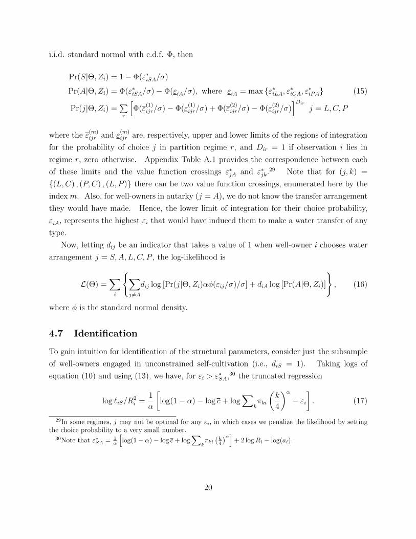
4.7 Identification

To gain intuition for identification of the structural parameters, consider just the subsample

of well-owners engaged in unconstrained self-cultivation (i.e., diS = 1). Taking logs of

equation (10) and using (13), we have, for εi > ε∗SA,30 the truncated regression

log `iS/R2i =

1

α

[log(1− α)− log c+ log

∑kπki

(k

4

)α− εi

]. (17)

29In some regimes, j may not be optimal for any εi, in which cases we penalize the likelihood by settingthe choice probability to a very small number.

30Note that ε∗SA = 1α

[log(1− α)− log c+ log

∑kπki(k4

)α]+ 2 logRi − log(ai).

20

Thus, α controls how fast irrigated area (scaled by well capacity) falls with variability in

water supply, c can be extracted from the intercept, and σ2 is the residual variance. Note

that, in general, error variances are not identified from discrete choices alone. For this reason,

it is crucial to have data on irrigated areas.

Of course, α is identified off of other moments of the data as well; in particular, the

shares of well-owners choosing different water arrangements conditional on their water supply

variability in addition to the average area irrigated under each arrangement. Similarly, the

water-buyer’s bargaining weight η and the leasing cost γ are identified off of the relative

shares of water transactions done on a per-irrigation or leasing basis and by differences in

average land area irrigated across transaction types. Finally, the transaction cost parameters

κL, κT , and β are identified off the proportion of well-owners who irrigate their full plot yet

choose not to transfer any water, how this proportion varies with average plot size in the

adjacency, as well as off of the relative proportions of leasers and water-sellers.

5 Results

5.1 Parameter estimates

Parameter estimates for the model are reported in Table 5 along with standard errors. The

estimates appear reasonable and extremely precise. In particular, α is considerable less than

one, whereas a value close to one would have implied little role for groundwater uncertainty.

The marginal inefficiency of leasing land, γ, is virtually zero, which means that the paucity of

lease activity in the data is largely driven by the high fixed transactions cost, κL (relative to

κT ). As expected, the coefficient β on average plot size in the adjacency is positive, indicating

that owners of borewells surrounded by larger plots (i.e., those more likely to have borewells

of their own) face higher transactions costs of arranging groundwater transactions.

Our estimates η = 0.935 and α = 0.218 translate (cf., definition of δ in Table 4) into a

3.1% efficiency loss due to holdup in the per-irrigation arrangement. The modesty of this

distortion suggests that water buyer and seller might be engaged in repeated interactions,

perhaps over multiple seasons, rather than in the one-shot bargaining game that we assume

in our stylized model.

21

5.2 Model fit

To assess model fit in the estimation sample, we predict for each borewell owner a probability

for each choice j = S,A, L, C, P . Also, for those borewell owners whose choice is either j = C

or P , we compute the expected irrigated area under the respective transfer arrangement

E[`ij|j] =

∫`j(εij)dΦij, (18)

where Φij is the appropriate truncated normal cdf of ε. We compute this latter expression

using Monte-Carlo integration by drawing εij from dΦij, calculating the corresponding `j(εij),

and averaging the result across draws.

Finally, we construct for every borewell owner, regardless of choice, a measure of predicted

groundwater market activity (in terms of area irrigated) as

E[`iT ] = Pri(C)E[`iC |C] + Pri(P )E[`iP |P ] (19)

where the Pri(j) are borewell-specific predicted choice probabilites.

Column 2 of Table 6 reports the results of these calculation in the estimation sample.31

The model does a decent job of predicting borewell owners’ choices of transfer arrangements

(L, C, and P ), but much less well on the S-A margin. Evidently, the reason for this is that

our likelihood function maximization is not just looking to match choice probabilities, but

also to fit area irrigated under each arrangement. The last row of the table shows that the

model indeed does reasonably well relative to the data in predicting E[`iT ].

Also in Table 6, we report predictions of our model (using parameters estimated on the

estimation sample) for borewells in the holdout sample. As one would hope, the model

indicates much less groundwater market activity in the drought-prone districts, capturing

well the virtual disappearance of the seasonal contract. Remarkably, the model fits the

probability of being unconstrained (P (S)) much better in the holdout sample than in the

estimation sample, but it also predicts higher prevalence of per irrigation contracts than is

otherwise found in the data.

31In this version of the paper, we do not perform the Monte Carlo integration over the conditional errordistribution, but simply set the error term to zero for each borewell owner. Results in Table 6 are preliminary.

22

5.3 Counterfactuals

Our first counterfactual asks what would happen to groundwater market activity in the

holdout districts if uncertainty is reduced to that prevailing in the estimation districts. To

perform this exercise, for each borewell in the holdout sample we draw a 5-tuple of πki at

random (with replacement) from the estimation sample and use it instead of the actual

vector of probabilities, rescaling λ (cf. equation 13) so as to keep wi constant. The analog is

also run by assigning each borewell in the estimation sample a vector of πki drawn at random

from the holdout sample.

Results for this mean-preserving change in σw using the estimation sample as the baseline

(column 3 of Table 6) and that using the holdout sample as the baseline (column 7) both

show a dramatic shift between seasonal contract and per-irrigation arrangement, but little

change in groundwater market activity (E[`iT ]). Thus, contractual choice appears to be far

more responsive to uncertainty levels than is the overall willingness to trade water.

We also performed the analogous exercise of replacing a with a randomly drawn counter-

part from the alternative sample. In contrast to the case of groundwater supply uncertainty,

differences in transactions costs across regions, which in our model are driven by differences

in a, have negligible impacts on groundwater transfer arrangements (see cols. 4 and 8 of

Table 6). In part, this reflects the small mean difference in average adjacency plot size across

estimation and holdout samples (0.45 acres).

Next, we consider a counterfactual in which borewell owners are endowed with plots of

essentially unlimited size. In other words, we ask what would happen in a world where land-

holdings were no longer fragmented. In terms of our model, land consolidation is tantamount

to having each borewell owner earn VS rather than Vj − κj under the best alternative water

arrangement.

On average, this hypothetical consolidation would lead to a 13.5% increase in irrigated

area and a 7.2% increase in economic surplus from dry-season cultivation in the four esti-

mation sample districts. Gains in the holdout sample districts would be negligible due to

the lack of extant groundwater markets. In figure 8, we plot counterfactual changes in both

irrigated area and surplus as a function of plot area adjusted for pipe-width (i.e., ai/r2i ). The

gains to consolidation are decreasing in adjusted plot size, as borewell owners with larger

plots are, of course, less compelled to engage in costly groundwater transactions.

23

6 Conclusion

We have developed a model of contractual arrangements, which, in the spirit of the transac-

tions cost literature, features a tradeoff between ex-post and ex-ante inefficiency. Long-term

contracts protect relationship-specific investment but are less flexible than spot contracts.

We have shown formally that, as payoff uncertainty rises, there is a shift from long-term to

spot contracting. Our structural estimates of the model using micro-data on area irrigated

under different groundwater transfer arrangements reveal a quantitatively important role for

uncertainty in shaping contractual form; less so in the development of groundwater mar-

kets. Given the distortions induced by this uncertainty, we find substantial gains from land

consolidation in terms of increased irrigated area and surplus, especially for those borewell

owners with the smallest plots.

While the specific context of groundwater is, of course, unique, we believe that this paper

has broader implications for how we think about markets in uncertain environments.

24

References

[1] Anderson, S. (2011). Caste as an Impediment to Trade. American Economic Journal:

Applied Economics, 3(1), 239-263.

[2] Banerji, A., J. V. Meenakshi, and G. Khanna (2012). Social contracts, markets and

efficiency: Groundwater irrigation in North India, Journal of Development Economics

98(2): 228-237.

[3] Binswanger, H. P. (1980). Attitudes toward risk: Experimental measurement in rural

India, American Journal of Agricultural Economics, 62(3):395-407.

[4] Carlton, D. W. (1979). Contracts, price rigidity, and market equilibrium. Journal of

Political Economy, 1034-1062.

[5] Cole, S., X. Gine, J. Tobacman, P. Topalova, R. Townsend, and J. Vickery (2013). Bar-

riers to household risk management: Evidence from India, American Economic Journal:

Applied Economics, 5(1): 104-35.

[6] Crocker, K. J., & Masten, S. E. (1988). Mitigating contractual hazards: Unilateral

options and contract length. RAND journal of economics, 327-343.

[7] Deaton, A. (1992). Understanding Consumption, Clarendon Lectures in Economics.

Oxford : Oxford University Press.

[8] Delavande, A. (2008). Pill, patch, or shot? subjective expectations and birth control

choice, International Economic Review, 49(3), 999-1042.

[9] Delavande, A., Gine, X., & McKenzie, D. (2011). Measuring subjective expectations

in developing countries: A critical review and new evidence, Journal of Development

Economics, 94(2), 151-163.

[10] Diamond, P. A., & Stiglitz, J. E. (1974). Increases in risk and in risk aversion. Journal

of Economic Theory, 8(3), 337-360.

[11] Economist (2009). When the Rains Fail, September.

[12] Fafchamps, M., & Pender, J. (1997). Precautionary saving, credit constraints, and irre-

versible investment: Theory and evidence from serniarid India, Journal of Business &

Economic Statistics, 15(2): 180-194.

25

[13] Fehr, E., Hart, O., & Zehnder, C. A. (2011). Contracts as Reference Points–

Experimental Evidence. American Economic Review, 101(2), 493-525.

[14] Fishman, R. M., Siegfried, T., Raj, P., Modi, V., & Lall, U. (2011). Over-extraction

from shallow bedrock versus deep alluvial aquifers: Reliability versus sustainability

considerations for India’s groundwater irrigation, Water Resources Research, 47(6).

[15] Foster, A., & Sekhri, S. (2008). Can expansion of markets for groundwater decelerate

the depletion of groundwater resource in rural India? unpublished manuscript, Brown

University.

[16] Gagnepain, P., Ivaldi, M., & Martimort, D. (2013). The cost of contract renegotiation:

Evidence from the local public sector, American Economic Review, 103(6): 2352-2383.

[17] Goldberg, V. P., & Erickson, J. R. (1987). Quantity and price adjustment in long-term

contracts: A case study of petroleum coke. Journal of Law and Economics, 369-398.

[18] Grossman, S. & Hart, O. (1986). The costs and benefits of ownership: A theory of

vertical and lateral integration, Journal of Political Economy, 691-719.

[19] Grout, P. (1984). Investment and wages in the absence of binding contracts: A Nash

bargaining approach, Econometrica, 52(2):449-60.

[20] Hart, O. (1995). Firms, contracts, and financial structure. Oxford University Press.

[21] Hart, O. (2009). Hold-up, asset ownership, and reference points, Quarterly Journal of

Economics, 124(1):267-300.

[22] Hart, O., & Moore, J. (1990). Property rights and the nature of the firm, Journal of

Political Economy, 98(6), 1119-1158.

[23] Hart, O. & Moore, J. (2008). Contracts as reference points, Quarterly Journal of Eco-

nomics, 123(1):1-47.

[24] Hoppe, E. I., & Schmitz, P. W. (2011). Can contracts solve the hold-up problem?

Experimental evidence. Games and Economic Behavior, 73(1), 186-199.

[25] Hubbard, R. G., & Weiner, R. J. (1992). Long-Term Contracting and Multiple-Price

Systems. Journal of Business, 177-198.

26

[26] Jacoby, H., & Mansuri, G. (2008). Land tenancy and non-contractible investment in

rural Pakistan, Review of Economic Studies, 75(3): 763-788.

[27] Jacoby, H., R. Murgai, and S. Rehman (2004). Monopoly power and distribution in

fragmented markets: The case of groundwater, Review of Economic Studies, 71(3):

783-808.

[28] Janakarajan, S. (1993). Economic and social implications of groundwater irrigation:

Some evidence from South India, Indian Journal of Agricultural Economics, 48(1): 65-

75.

[29] Joskow, P. L. (1987). Contract duration and relationship-specific investments: Empirical

evidence from coal markets. American Economic Review, 168-185.

[30] Keane, M. P., & Wolpin, K. I. (2007). Exploring the usefulness of a nonrandom holdout

sample for model validation: Welfare effects on female behavior. International Economic

Review, 48(4), 1351-1378.

[31] Kimball, M. (1990). Precautionary saving in the small and in the large, Econometrica,

58(1): 53-73.

[32] Klein, B., Crawford, R. G., & Alchian, A. A. (1978). Vertical integration, appropriable

rents, and the competitive contracting process. Journal of law and economics, 297-326.

[33] Lafontaine, F. and Slade, M. E., (2012), Inter-Firm Contracts in Gibbons, R. and

Roberts, J. eds., Handbook of Organizational Economics. Princeton University Press.

[34] Mahajan, A., Tarozzi, A., & Yoong, J. (2012). Bednets, information and malaria in

Orissa, unpublished manuscript.

[35] Mahajan, A., & Tarozzi, A. (2012). Time inconsistency, expectations and technology

adoption: The case of insecticide treated nets, unpublished manuscript.

[36] Masten, S. E., & Crocker, K. J. (1985). Efficient adaptation in long-term contracts:

Take-or-pay provisions for natural gas. American Economic Review, 1083-1093.

[37] New York Times (2006). India Digs Deeper, but Wells are Drying Up, September.

[38] Polinsky, A. M. (1987). Fixed Price versus Spot Price Contracts: A Study in Risk

Allocation. Journal of Law Economics & Organization, 3, 27.

27

[39] Sekhri, S. (2013). Wells, water, and welfare: The impact of access to groundwater on

rural poverty and conflict. American Economic Journal: Applied Economics.

[40] Shah, T. (2007). The groundwater economy of South Asia: an assessment of size, sig-

nificance and socio-ecological impacts. The agricultural groundwater revolution: Oppor-

tunities and threats to development, 7-36.

[41] Shah, T. (2009). Taming the anarchy: Groundwater governance in South Asia. Re-

sources for the Future, Washington DC.

[42] Williamson, O. E. (1971). The vertical integration of production: market failure con-

siderations. American Economic Review, 112-123.

[43] World Bank (2005). India’s water economy: Bracing for a turbulent future. Washington

DC: The World Bank.

28

𝑟∗ 𝑟𝐶 𝑟𝑃 𝑟𝑆 Mean preserving spread

Surplus

𝑉𝑆 𝑉𝐶

𝑉𝐴

𝑉𝑃

Long-term contract dominates

Spot contract dominates

Autarky dominates

Unconstrained self-cultivation dominates (ℓ𝑺 < 𝒂)

Competitive spot market (unattainable)

Figure 1: Long-term versus spot contracts and uncertainty

29

010

2030

0 .2 .4 .6 0 .2 .4 .6

Estimation Sample (N=1649) Holdout Sample (N=774)

Den

sity

CV end-of-season flowNote: Estimation sample drawn from East Godavari, Guntur, Kadapa, and West Godavari districts; holdout sample from drought-prone Anantapur and Mahabubnagar districts.

Figure 2: Borewell-level groundwater supply uncertainty

30

0.2

.4.6

.81

prop

ortio

n of

plo

ts w

ith b

orew

ell

0 2 4 6 8 10plot area (acres)

95% CI local cubic polynomial fit cum. distribution function

Figure 3: Presence of a borewell and area of plot

.2.4

.6.8

1pr

opor

tion

of p

lots

with

bor

ewel

l

0 2 4 6 8 10plot area (acres)

95% CI unconditional conditional plot area/tot. area owned.

Note: Conditional local cubic polynomial fit partials out dummies for the deciles of totalland area owned

Figure 4: Presence of a borewell and area of plot controlling for wealth

31

0.1

.2.3

.4pr

opor

tion

of p

lots

left

entir

ely

fallo

w in

rab

i

0 2 4 6 8 10plot area (acres)

95% CI local cubic polynomial fit

Figure 5: Dry-season fallow and area of plot

32

0.2

.4.6

.81

bore

wel

l are

a/to

tal a

rea

0 2 4 6 8 10average plot area (acres)

Borewell Density and Average Plot Size in Adjacency

0.2

.4.6

tran

sact

ions

/tota

l plo

ts

0 2 4 6 8 10average plot area (acres)

Frequency of Groundwater Transfers and Average Plot Size in Adjacency

95% CI local cubic polynomial fit

Figure 6: Borewell density, groundwater transfers, and average plot size

33

𝑒𝜀𝐿𝑃∗

𝑒𝜀𝐿𝐶∗

𝑒𝜀𝐶𝐴∗

𝑒𝜀

𝑒𝜀

𝑒𝜀𝑆𝐴∗

𝑉𝐿 − 𝜅𝐿

𝑉𝑃 − 𝜅𝑇

𝑉𝐶 − 𝜅𝑇

𝑉𝐴

𝑉𝑆

P L C A S

den

sity

va

lue

Figure 7: A possible partition of the error-space

34

02

46

810

% c

hang

e in

sur

plus

-50

510

1520

% c

hang

e in

sur

plus

0 2 4 6 8borewell plot area / pipe radius squared

% change in area irrigated% change in surplus

Figure 8: Impact of hypothetical land consolidation

35

Table 1: Characteristics of Adjacent Plots

Estimation Sample Holdout Sample

Mean number of adjacent plots per adjacency 3.39 3.59

Mean area of adjacent plots (acres) 2.95 3.34

% of adjacent plots left fallow in rabi 2 38

% of adjacent plots irrigated in rabi by• reference borewell 42 15

of which, % irrigated under-joint ownership of reference borewell 22 95-land lease 6 3-water sale 71 2

• own borewell 46 46• other borewell 14 2

% of adjacent plots owned by• brother of reference borewell owner 8 21• other relative 10 11• unrelated member of same caste 50 33• unrelated person of different caste 32 35

Number of plots 4943 2350

36

Table 2: Precautionary Planting and Risk Aversion

Subjective measure (Y s) Objective measure (Y o)

(1) (2) (3) (4) (5) (6)

(a) Baseline

log(CV) -0.0849*** -0.0678*** -0.136*** -0.524*** -0.513*** -0.209***(0.0151) (0.0157) (0.0197) (0.0344) (0.0363) (0.0417)

log(pipe width) -0.0657*** -0.0543*** 0.0340 0.415*** 0.488*** 0.182***(0.0178) (0.0186) (0.0207) (0.0455) (0.0531) (0.0585)

(b) RISK1

log(CV) -0.0997** -0.0842** -0.137*** -0.405*** -0.390*** -0.116(0.0413) (0.0415) (0.0420) (0.0922) (0.0929) (0.0864)

log(pipe width) -0.0656*** -0.0540*** 0.0341 0.410*** 0.482*** 0.181***(0.0179) (0.0187) (0.0207) (0.0456) (0.0532) (0.0586)

RISK1 0.00390 0.00408 0.000547 -0.0495* -0.0510* -0.0296(0.0128) (0.0129) (0.0128) (0.0292) (0.0294) (0.0266)

log(CV)×RISK1 0.00243 0.00268 0.000194 -0.0190 -0.0197 -0.0154(0.00657) (0.00656) (0.00654) (0.0151) (0.0151) (0.0138)

(c) RISK2

log(CV) -0.0543 -0.0301 -0.0912** -0.422*** -0.401*** -0.109(0.0367) (0.0372) (0.0383) (0.0757) (0.0763) (0.0733)

log(pipe width) -0.0664*** -0.0552*** 0.0336 0.412*** 0.486*** 0.181***(0.0178) (0.0186) (0.0207) (0.0455) (0.0531) (0.0585)

RISK2 -0.0955 -0.117 -0.136 -0.355 -0.390* -0.322(0.107) (0.107) (0.106) (0.222) (0.224) (0.204)

log(CV)×RISK2 -0.0471 -0.0580 -0.0709 -0.154 -0.169 -0.157(0.0550) (0.0551) (0.0544) (0.118) (0.118) (0.108)

Controls No Yes Yes No Yes YesDistrict dummies No No Yes No No YesObservations 2,396 2,388 2,388 2,417 2,409 2,409

Notes: Robust standard errors in parentheses adjusted for clustering on borewell (*** p<0.01, ** p<0.05,

* p<0.1). CV is the coefficient of variation of end-of-season well flow; RISK1 is a self-assessed ranking of

risk tolerance; RISK2 is an index of marginal willingness-to-pay for risk based on a Binswanger lottery.

Unreported controls are as follows: pump horse-power, log of well depth, number of other borewells

within 100 meters, dummy for presence of recharge source.

37

Table 3: Descriptive Statistics

Estimation Sample Holdout Sample

Choice j N `j a N `j a

S =unconstrained 184 6.64 11.93 466 4.07 9.25(6.00) (10.33) (2.64) (6.41)

A =autarky 362 − 8.33 288 − 4.59− (15.16) − (2.70)

L =leasing 97 3.07 4.77 14 1.71 4.05(3.78) (3.24) (1.46) (2.93)

C =seasonal contract 642 3.11 6.07 1 1.00 2.00(2.73) (7.05) (0.00) (0.00)

P =per-irrigation sale 361 1.89 4.25 4 1.68 2.75(1.63) (2.72) (0.84) (1.19)

Total 1646 − 6.75 773 − 7.37(9.45) (5.74)

Notes: Sample means (standard deviations).

Table 4: Theoretical Solutions for Irrigated Area and Economic Surplus

Choice j Area (`j) Surplus (Vj)

S =unconstrained(

1−αcEwα

)1/α αc1−α`S

A =autarky a a1−αEwα − ca

L =leasing (1 + γ)−1/α`S − a (1 + γ)1−1/αVS + γca

C =seasonal contract `C solves EΩα−1 = 1 αc1−α [EΩα + α`C/a− (1− α)]

P =per-irrigation sale η1/α`S − a δVS

Notes: Ω = 1a

[w(

1−αc

)1/α − `C]

and δ = 1−η(1−α)α

η1/α−1.

38

Table 5: Parameter Estimates

Parameter Estimate Std. Error

α 0.218 0.0307c 0.731 0.0371γ 0.001 0.0032η 0.935 0.0096κL 0.320 0.1091κT 0.066 0.0118β 0.133 0.0454σ 0.232 0.0333

Mean log-likelihood 2.753

Table 6: Model Predictions

Estimation Sample Holdout Sample

Data Model ∆σw ∆a Data Model ∆σw ∆a

P r(S) 11.05 30.09 30.85 30.09 60.28 61.38 60.58 61.38

Pr(A) 21.92 12.26 13.95 12.42 37.26 14.77 13.69 14.72

Pr(L) 5.89 5.44 5.48 5.13 1.81 0.14 0.15 0.16

Pr(C) 39.40 32.17 9.04 32.00 0.13 5.68 18.75 5.61

Pr(P ) 21.74 20.04 40.67 20.37 0.52 18.03 6.83 18.12

E[`C |C] 3.11 4.81 3.37 4.81 1.00 0.00 0.00 0.00

E[`P |P ] 1.89 3.91 3.73 3.91 1.68 0.79 0.83 0.79

E[`T ] 1.11 1.99 2.01 2.03 0.01 0.08 0.07 0.08

Notes: Data represents raw means from the respective sample, Model the mean

prediction, ∆σw the mean prediction when each borewell in the estimation (hold-

out) sample is assigned a σw drawn at random from the holdout (estimation) sam-

ple, and ∆a the mean prediction when each borewell in the estimation (holdout)

sample is assigned an a drawn at random from the holdout (estimation) sample.

39

Appendix

A Proof of Proposition 2

We begin by proving that under any water-transfer arrangement economic surplus, Vj(r)

j = S,A,C, P , strictly diminishes with mean-preserving increases in uncertainty r. But

first, we paraphrase a result from Diamond and Stiglitz (1974, p. 340, fn. 8). For any twice

continuously differentiable function h(w)∫h(w)ψrdw =

∫hww(w)T (w, r)dw, (A.1)

where ψ is a p.d.f., ψr is its partial derivative with respect to r, and T (w, r) is a nonnegative

function defined in equation (5) of Diamond and Stiglitz (1974).

Lemma 1 If g is strictly concave, then V ′j (r) < 0 for j = S,A,C, P .

Proof. (i) VS: Differentiating definition 2 and using the envelope theorem yields

V ′S(r) = `S

[∫f(w/`S)ψrdw − c

]. (A.2)

Since, by (A.1) and the concavity of f , the first term in square brackets is negative, V ′S(r) < 0.

(ii) VA: Follows from (A.2) with `S replaced by a.

(iii) VC : As noted in fn. 11, VC = aE[f(w−τC

a)− c

]+ `C

[f( τC

`C)− c

]. Differentiating with

respect to r and using the envelope theorem leads to an expression analogous to (A.2).

(iv) VP : Given the discussion in fn. 11,

VP = aE

[f(w − τPa

)− c]

+ `P

[f(τP`P

)− c]

(A.3)

= (a+ `P )E

[f(

w

a+ `P)− c

],

where the second line follows from the ex-post efficiency condition f ′( τP`P

) = f ′(w−τPa

). Dif-

40

ferentiating with respect to r in this case yields

V ′P (r) = E

[g

(w

a+ `P

)− c]∂`P∂r

+ (a+ `p)

[∫f

(w

a+ `P

)ψrdw − c

](A.4)

= c

(1

η− 1

)∂`P∂r

+ (a+ `p)

[∫f

(w

a+ `P

)ψrdw − c

],

where the second line uses equation (7). In the case of the per-irrigation arrangement, a

precise analog to Proposition 1 applies. Thus, given that g is concave, ∂`P/∂r < 0. The first

term of (A.4) must, therefore, be negative and, using (A.1) again, the second term must also

be negative.

Proof of proposition 2: (a) Proposition 1 implies that for sufficiently large r, say

rS, `S = a and, hence, VS(rS) = VA(rS). Recall that under perfect certainty, VC(0) =

VS(0) > VA(0). Given τC(0) < wL (see fn. 12) and lemma 1, VC is continuously decreasing

in r until it equals VA at some r = rC . Now use equation (7) under perfect certainty to

define η = c/g(w/a). For η ≤ η, `P = 0 ∀r and, consequently, VP (r, η) = VA(r) ∀r and, in

particular, for r = 0. Define rP (η) as the solution to

VP (rP (η), η) = VA(rP (η)). (A.5)

Thus, clearly, rP (η) = 0. Recall, also, that VP (r, 1) = VS(r) ∀r, so rP (1) = rS. To prove

part (a), it is sufficient to show that rP (η) ∈ (rC , rS) for some η. This is so because

VP (0, η) < VC(0) for all η < 1 and, therefore, by continuity, the functions VC(r) and VP (r, η)

must cross at r∗ < rC if indeed rP (η) > rC (see figure 1).

Thus, it is sufficient to show that r′P (η) > 0 so that as η is increased from η to 1 rP (η)

eventually exceeds rC . Differentiating equation (A.5) with respect to η, substituting from

equation (7), and rearranging gives

c

(1

η− 1

)∂`P∂η

+

[∫h (w)ψrdw

]r′P (η) = 0 (A.6)

where h(w) = (a + `P )f( wa+`P

) − af(wa

). Since ∂`P/∂η < 0, and given (A.1), we have that

sign(r′P (η)) = −sign(hww(w)). Differentiating h(w) twice, we get

hww(w) =1

a+ `P

[f ′′(

w

a+ `P

)− a+ `P

af ′′(wa

)](A.7)

41

A Taylor expansion around `P = 0 gives f ′′(

wa+`P

)≈ f ′′

(wa

)− w`P

a2f ′′′(wa

). Substituting into

equation (A.7) and rearranging yields

hww(w) ≈ −`Pa(a+ `P )

[f ′′(wa

)+w

af ′′′(wa

)]. (A.8)

Since the term in square brackets is just −g′′(w/a), the concavity of g ensures that hww < 0

and hence that r′P (η) > 0.(b) Having just established that rP (η) > rC for some η ∈ (η, 1), it must be true that

VP (r, η) > VC(r) over the interval (r∗(η), rP (η)).

B Additional Figures

42

0.2

.4.6

Bor

ewel

l sha

re o

f irr

igat

ed a

rea

1970 1980 1990 2000 2010

All India Andhra Pradesh6 surveyed districts in AP

Source: ICRISAT district level database.(All India covers 17 major states, excluding W. Bengal and Maharashtra for lack of data)

Figure B.1: Rising Importance of Borewell Irrigation in India

43

HYDROGRAPH OF MONTHLY AVERAGE GROUND WATER LEVEL AND

RAINFALL IN ANDHRA PRADESH

0

50

100

150

200

250

300

350

400

May

-98

Jul-

98

Sep

-98

No

v-9

8

Jan

-99

Mar

-99

May

-99

Jul-

99

Sep

-99

No

v-9

9

Jan

-00

Mar

-00

May

-00

Jul-

00

Sep

-00

No

v-0

0

Jan

-01

Mar

-01

May

-01

Jul-

01

Sep

-01

No

v-0

1

Jan

-02

Mar

-02

May

-02

Jul-

02

Sep

-02

No

v-0

2

Jan

-03

Mar

-03

May

-03

Jul-

03

Sep

-03

No

v-0

3

Jan

-04

Mar

-04

May

-04

Jul-

04

Sep

-04

No

v-0

4

Jan

-05

Mar

-05

May

-05

Jul-

05

Sep

-05

No

v-0

5

Jan

-06

Mar

-06

May

-06

Jul-

06

Sep

-06

No

v-0

6

Jan

-07

Mar

-07

May

-07

Rain

fall

in

m

m .

0.00

1.00

2.00

3.00

4.00

5.00

6.00

7.00

8.00

9.00

10.00

11.00

12.00

13.00

14.00

15.00

16.00

Dep

th t

o w

ate

r le

vel

m b

gl

Rainfall Water level Trend

TREND LINE

Fig.9

Source: Govt. of Andhra Pradesh, Ground Water Dept. (2007)

Figure B.2: Average depth to water table in Andhra Pradesh

44

.4.4

5.5

.55

.6S

hare

of f

arm

s <

1 h

a

1975 1985 1995 2005

All India Andhra Pradesh6 surveyed districts in AP

Source: ICRISAT district level database.(All India covers 19 major states)

Figure B.3: Increasing Land Fragmentation in India

45