Market valuation and acquisition quality: Empirical evidence

Christa H.S. Bouwman* Kathleen Fuller**

Amrita S. Nain***

September 2006

Review of Financial Studies, Forthcoming

Abstract

Existing research shows that significantly more acquisitions occur when stock markets are booming than when markets are depressed. Rhodes-Kropf and Viswanathan (2004) hypothesize that firm-specific and market-wide (mis-)valuations lead to an excess of mergers, and these will be value-destroying. This paper investigates whether acquisitions occurring during booming markets are fundamentally different from those occurring during depressed markets. We find that acquirers buying during high-valuation markets have significantly higher announcement returns but lower long-run abnormal stock and operating performance than those buying during low-valuation markets. We investigate possible explanations for the long-run underperformance and conclude it is consistent with managerial herding. JEL Classification: G34 * Case Western Reserve University, 10900 Euclid Avenue, 362 Peter D. Lewis Building, Cleveland, OH 44106. Tel.: 216-368-3688. E-mail: christa.bouwman@case.edu. ** University of Mississippi, 244 Holman Hall, University, MS 36877. Tel.: 662-915-5463. E-mail: kfuller@bus.olemiss.edu. *** McGill University, 1001 Sherbrooke Street West, Montreal, Quebec, H3A 1G5, Tel.: 514-398-8440. E-mail: amrita.nain@mcgill.ca. The authors thank an anonymous referee and Matt Spiegel for helpful suggestions, and Arnoud Boot, Sreedhar Bharath, Sugato Bhattacharyya, Jayant Kale, Gautam Kaul, E. Han Kim, Marc Lipson, Jeffry Netter, David Robinson, Nejat Seyhun, Anjan Thakor, ‘Vish’ Viswanathan, Guojun Wu, participants of the University of Michigan Business School finance department brown bag seminar, University of Mississippi 2004 seminar series, University of Missouri-Kansas City 2004 seminar series, the 2002 Estes Park Conference, and the 2003 Financial Management Association Conference for useful comments.

1

A sizeable stream of theoretical and empirical research on mergers and acquisitions (M&A) reveals that

takeover activity comes in waves; announcement-day returns are significantly positive for target

shareholders but may be significantly positive or negative for bidder shareholders depending on the mode

of acquisition, method of payment and type of target; and post-acquisition returns to acquiring

shareholders are higher for cash offers and tender offers than for stock offers and mergers.1 More recent

research explores the possible link between M&A activity and stock prices. Jovanovic and Rousseau

(2001) show that periods of high merger activity are correlated with high market valuations.2 Rhodes-

Kropf and Viswanathan (2004) develop a model in which firm-specific and market-wide misvaluations

can cause merger waves. Shleifer and Vishny (2003) model the impact of market valuations on the

decision to acquire, the method of payment, acquirer performance, and the occurrence of merger waves.

Consistent with these theories, Rhodes-Kropf, Robinson and Viswanathan (2005) find strong empirical

evidence that market (mis-)valuation affects merger activity. Moreover, there is plenty of anecdotal

evidence, including the following quote, that acquisition decisions are influenced by market valuations.

“Why did CEOs do so many deals […]? The bull market was a big reason, of course. Executives

were brimming with confidence and rich stocks.” (Business Week Oct. 14, 2002, p. 68)

Theory suggests that market valuations may not only affect merger activity, but also the quality of

completed deals. Using a model where stock prices have both a firm-specific and a market-/industry-

wide component, Rhodes-Kropf and Viswanathan (2004) show that (mis-)valuation leads to ex-post

mistakes that are correlated with (mis-)valuation at the market/industry level. When market/industry

valuation is low, targets will only accept bids if synergy estimates outweigh the negative information in

the stock price. When market/industry valuation is high, targets filter out too little of the market-wide

effect, and hence, bids tend to appear more attractive and targets are more prone to accept. Thus, from

the acquiring-firm shareholders’ perspective, the best deals (on average) are initiated when markets are

1 For a discussion of merger waves, see Andrade, Mitchell and Stafford (2001), and Holmstrom and Kaplan (2001). For evidence on announcement-day returns and post-acquisition returns, see Asquith (1983), Jensen and Ruback (1983), Dennis and McConnell (1986), Bradley, Desai and Kim (1988), Franks, Harris and Titman (1991), Agrawal, Jaffe and Mandelkar (1992), Loughran and Vijh (1997), Rau and Vermaelen (1998), Bruner (2002), and Fuller, Netter and Stegemoller (2002). 2 As noted in Nelson (1959), the idea that stock prices influence merger activity is not new.

2

depressed while worse deals are initiated when markets are booming. Goel and Thakor (2005) also

predict that mergers undertaken during bull markets involve smaller synergies than those undertaken

during bear markets, and hence will be of lower quality. If deals initiated when markets are booming in

fact do create less value for acquiring-firm shareholders than deals initiated when markets are depressed,

managers may want to refrain from undertaking acquisitions during boom periods. The goal of this paper

is to shed light on these issues by empirically addressing the following question: Are acquisitions that are

announced when the market is booming fundamentally different from those that are initiated during

market troughs? Specifically, we want to investigate whether acquisitions undertaken during booming

stock markets are of poorer quality than those undertaken during depressed markets, and if so, why?

Using a sample of 2,944 acquisitions announced between January 1, 1979 and December 31,

2002, we examine if fundamental quality differences exist between acquisitions announced when market

valuations are high and those announced when market valuations are low. We split our sample period

into times of high, neutral and low market valuations, and compare the performance of firms that

announce acquisitions under those different market circumstances. We use several stock and operating

performance measures. We examine acquiring firms’ short-run stock performance (three-day cumulative

abnormal returns) and long-run stock performance (two-year buy-and-hold abnormal returns and

calendar-time portfolio returns) to see whether the market’s initial reaction is consistent with the

acquirers’ long-run stock performance. We also analyze long-run operating performance (two-year

abnormal return on operating income) of acquirers to find out whether it is consistent with our stock

performance results. We examine the performance of high-, neutral- and low-market acquisitions in a

univariate setting and in a multivariate regression framework where we control for other factors that may

affect acquisition performance, including method of payment, acquisition type (tender / merger), the

relative size of the acquisition, and acquirer market-to-book (M/B). Both approaches yield similar results.

The definition of what constitutes a market boom or trough is critical. We use seven alternative

methods to classify time periods into high-, neutral- and low-valuation markets and refer to deals initiated

during those periods as high-, neutral- and low-market acquisitions, respectively. Our main classification

method is based on the price-earnings (P/E) ratio of the S&P500 index. Since the market P/E has steadily

3

increased over our sample period, we use a detrended version rather than the actual market P/E to ensure

that low-valuation (high-valuation) markets do not simply correspond to the first (second) half of our

sample period. Alternative classification methods use the level of the S&P500 index, the M/B ratio of the

overall market, and the M/B ratio of the acquirer’s industry. Our results are generally similar. One

potential concern is that our market valuation measures simply reflect firm valuation; however, our results

hold even after explicitly taking firm valuations into account.

Our main findings are as follows. Bidder announcement returns are insignificantly negative for

acquisitions initiated in high-valuation markets but significantly negative for deals announced in low-

valuation markets, and the difference between the two is significant. Interestingly, although firms that

acquire when markets are booming produce significantly higher announcement returns for their

shareholders than firms that acquire when markets are depressed, they generate significantly lower long-

run abnormal stock performance for their shareholders, as measured by buy-and-hold abnormal returns

(BHARs) and calendar-time abnormal returns.3 While this pattern may also be consistent with short-term

momentum followed by long-run stock price reversals, we show that the underperformance of high-

market acquisitions is not driven by reversals. Furthermore, high-market acquirers have significantly

lower (i.e., more negative) long-run operating performance, as measured by abnormal returns on

operating income, than low-market acquirers. Thus, our main findings suggest that low-market

acquisitions are fundamentally different from high-market acquisitions.

Another interesting finding of our paper concerns previously documented evidence that

acquisitions made with cash deliver positive long-run abnormal stock returns for acquirers (see Loughran

and Vijh, 1997; and Rau and Vermaelen, 1998). We find that while cash acquisitions undertaken in the

1980s generated significantly positive long-run abnormal stock returns for bidder shareholders, cash

acquisitions undertaken in the 1990s produced significantly negative long-run abnormal returns. This

poor performance of cash acquisitions in the 1990s was driven by the significant underperformance of

high-market cash acquisitions that accounted for 60% of all cash acquisitions in that decade. The

3 The BHAR results hold regardless of whether the announcement month return is included in the analysis. In fact, our results are even stronger if we include the announcement month returns: the positive performance of low-market stock acquisitions is significant in this case.

4

experience of high-market cash acquirers in the 1990s suggests that when stock prices are soaring,

making cash offers may destroy shareholder value.

In the second part of the paper, we explore reasons why high-market acquirers underperform

relative to low-market acquirers in the long run. We examine three possible explanations: overpayment,

market timing, and managerial herding. We discuss these in turn. First, managers may be overpaying for

targets during high-valuation markets. However, we do not find evidence consistent with overpayment:

the average bid premium is significantly lower in high-valuation markets than in low-valuation markets.

The second explanation for the underperformance of high-market acquirers we explore is market

timing. During stock markets booms, the enthusiasm to pay with overvalued stock may increase the

number of stock acquisitions, and signaling theory suggests that these are likely to experience subsequent

stock-price corrections. Consistent with this, our data show that there are far more stock acquisitions

during high-valuation markets than during low-valuation markets. However, when we partition high-

market acquirers based on whether they announce a stock acquisition when their stock price is close to an

annual high (market timers), we find that market timers have significantly higher BHARs and

insignificantly higher calendar-time returns. Thus, it does not seem that market timing can explain why

high-market acquirers perform relatively poorly. Four additional factors suggest market timing is not a

sufficient explanation for our results. First, we find that the operating performance of high-market

acquirers is also significantly less than that of low-market acquirers. Second, the operating performance

of market timers is statistically indistinguishable from that of acquirers who do not time the market.

Third, cash acquisitions announced during high-valuation markets (39% of high-market acquisitions) also

significantly underperform in the long run: these acquisitions are not attempts to time the market and do

not signal overvaluation of acquirer stock. Fourth, the performance of high-market cash acquirers whose

stock prices are close to a recent peak is not significantly different from that of high-market cash

acquirers whose stock prices are not close to a peak.

The third explanation for the underperformance of high-market acquirers we investigate is the

possibility of managerial herding during merger waves that accompany booming stock markets. Existing

models of herding suggest that firms who move later in a merger wave are likely to perform poorly

5

relative to firms that move earlier. Persons and Warther (1997) present a fully rational model which

predicts that innovation waves tend to end on a sour note because firms stop adopting a technology only

after observing the poor experience of recent adopters. Rhodes-Kropf and Viswanathan (2004) also

suggest that merger waves end only after the market learns from the bad experience of previous acquirers.

According to these models, acquisitions occurring late in a merger wave are more likely to be value

destroying. Other models (see, for example, Banerjee (1992) and Bikhchandani, Hershleifer and Welch

(1998)) suggest that if a handful of firms consecutively adopt an action, subsequent firms will ignore their

own private signals about the value of that action and defer to the actions of predecessors. As a result, if

the state of the world is stochastically changing, these models also seem to suggest that, by ignoring their

own signals, late movers are likely to make unprofitable acquisitions even though they have the benefit of

information implicit in the actions of predecessors. Thus, if managerial herding is the explanation for the

underperformance of high-market acquisitions, then this underperformance is likely to be driven by firms

that acquire later in a high-valuation merger wave.

We perform various tests and conclude that managerial herding is a likely explanation for the

underperformance of high-market acquirers. We divide the sample of acquirers buying during high-

valuation markets into early and late movers, and find that early acquirers show no abnormal stock

performance, as measured by BHARs, in the two years following the acquisition announcement, while

late acquirers underperform. Difference-in-means tests indicate that early acquirers have significantly

higher BHARs than late movers. These results hold for both cash and stock acquisitions, and cannot be

explained by industry effects or observable differences in acquirer and target characteristics. We also find

that the calendar-time returns and operating performance of early acquirers are both significantly better

than those of late acquirers during high-valuation periods. Recognizing that merger waves are a

phenomenon of booming stock markets, we repeat our analysis for stock acquisitions announced during

low-valuation markets and expect to see no difference in the performance of early and late movers. Our

(stock) performance findings confirm this. An alternative approach where we split high-market acquirers

into early, middle and late movers, yields similar results: early movers show significantly better

performance than middle and late movers. On the basis of these results, we conclude that the overall

6

underperformance of high-market acquirers is attributable to firms that acquire later in high-valuation

markets and this underperformance is consistent with the existence of managerial herding.

Our paper is related to Loughran and Vijh (1997), Rau and Vermaelen (1998), Ang and Cheng

(2006), Dong, Hirshleifer, Richardson, and Teoh (2006), and Rhodes-Kropf, Robinson, and Viswanathan

(2005). Loughran and Vijh (1997) find that the long-run performance of acquirers using stock is worse

than that of acquirers using cash and that tender offers have significantly positive long-run returns while

mergers have significantly negative long-run returns. Rau and Vermaelen (1998) find that the acquirer’s

M/B at the time of the acquisition affects its long-term stock performance; specifically, firms with low

book-to-market ratios underperform in the long run. In this paper, we control for the method of payment

and the mode of acquisition (as in Loughran and Vijh, 1997), and for acquirer M/B (as in Rau and

Vermaelen, 1998), and focus on the impact of market-wide valuations on acquirer performance in the

short and long run. Ang and Cheng (2006) and Dong, Hirshleifer, Richardson, and Teoh (2006) provide

evidence that market misvaluation impacts the volume of takeovers and the behavior of participants in

takeover contests. In both papers, market valuation is defined on a firm-specific level (M/B ratios),

whereas we define market valuation as the valuation of the market as a whole or the valuation of the

industry in which an acquirer is active, while controlling for firm-specific valuations. Finally, Rhodes-

Kropf, Robinson, and Viswanathan (2005) examine if firm-specific and market-wide (mis-)valuations

cause merger waves. In this paper, we are not concerned with the causes of merger waves.

The rest of the paper is organized as follows. Section 1 describes the data, Section 2 discusses

our methodology, and Section 3 presents our results. Section 4 examines possible explanations for our

results. Robustness issues are addressed in Section 5. Section 6 summarizes and concludes.

1. Data

In this section, we describe our sample, explain our classification into high-, neutral- and low-valuation

markets, and provide summary statistics.

7

1.1 Description

Our sample contains completed tender offers and mergers gathered from the Securities Data

Corporation’s (SDC) U.S. Mergers and Acquisitions Database that were announced between January 1,

1979 and December 31, 2002. We identify 2,944 acquisitions that meet the following conditions:

1. The acquirer is a U.S. firm listed on the NYSE, NASDAQ or AMEX.

2. The target is not a subsidiary.4

3. Daily acquirer return data are available for three days around the announcement date and the

following acquirer data are available for two years following the acquisition: market equity (as of

June of each year), the book-to-market ratio (as of December of each year) and monthly return data.

4. The transaction value is $50 million or more.

5. The acquirer obtains at least 50% of the shares of the target.

6. The closing share price of the acquirer for the month before the announcement is at least $3 (see

Loughran and Vijh, 1997). This eliminates firms that are very small or in distress.

7. The method of payment is cash, stock or a mixture of the two. As in Fuller, Netter and Stegemoller

(2002) and Heron and Lie (2002), we define a cash acquisition as any acquisition in which the total

transaction value was paid in cash, non-convertible debt or non-convertible preferred stock. We

define a stock acquisition as any acquisition in which the total transaction value was paid in common

stock and options, warrants, rights or convertible debt. Acquisitions with some combination of cash

and stock are defined as mixed payment acquisitions.

1.2 Classification of High-, Neutral- and Low-Valuation Markets

We want to examine whether acquisitions announced in high-valuation markets are fundamentally

different from acquisitions announced in low-valuation markets. Therefore, how we measure the

market’s valuation is very important. To ensure that our conclusions are not based on one particular

definition of market valuation, we use seven alternative definitions. Here we discuss our base

specification which is based on the P/E ratio of the S&P500 and uses monthly data. Alternative

4 Hansen and Lott (1996) and Fuller, Netter and Stegemoller (2002) justify the exclusion of subsidiary acquisitions.

8

definitions, which use quarterly data, or are based on the level of the S&P500, the M/B ratio of the overall

stock market, or the M/B ratio of the industry in which the acquirer operates, are covered in Section 5.2.

Our base specification classifies the stock market in a particular month as a high-, neutral- or low-

valuation market based on the P/E ratio of the S&P 500 (and we refer to acquisitions that were announced

during that month as high-, neutral- or low-market acquisitions).5 At first glance, it seems as if we could

simply use the market’s actual P/E ratio in a particular month to classify the market. However, the P/E

ratio of the market has trended upwards over time, and hence, this approach would lead us to classify all

acquisitions that occurred in the first half of the sample period (1979-1991) as low-market acquisitions,

and all acquisitions that were announced in the second half (1992-2002) as high-market acquisitions.

Since the 1980s contained a merger wave while only the latter half of the 1990s is commonly referred to

as a merger wave (see Andrade, Mitchell and Stafford, 2001), our approach must avoid this problem.

First, we detrend the market P/E by removing the best straight-line fit from the P/E of the month

in question and the five preceding years.6 Second, each month is categorized as above (below) average if

the detrended market P/E of that month was above (below) this past five-year average. Third, the top half

of the above-average months are then classified as high-valuation markets and the bottom half of the

below-average months are classified as low-valuation markets. All other months are classified as neutral-

valuation markets.

Using this approach, half of all months are classified as neutral-valuation markets, while high-

valuation and low-valuation markets combined constitute the other half. Alternatively, one could argue

that the number of high-, neutral-, and low-valuation markets should be the same, or that markets should

only be classified as high-valuation (low-valuation) if the detrended P/E ratio in a particular month is

sufficiently far (e.g. 0.5 standard deviation) above (below) the past five-year average. We show in

Section 5.2 that our results are robust to these alternative specifications.

5 We thank Bob Shiller for providing the P/E data on his website (http://www.irrationalexuberance.com/index.htm). 6 Our results are robust to reasonable changes in the length of the historical data used to detrend the P/E ratio.

9

1.3 Summary Statistics

From January 1979 – December 2002, we find 85 high-valuation, 59 low-valuation and 144 neutral-

valuation markets.7 Table 1 shows that there are slightly more acquisitions during high-valuation markets

than during low-valuation markets. In terms of total deal value, 42% (33%) of all acquisition dollars are

spent in high- (low-) valuation markets. Moreover, about 46% of high-market acquisitions are for stock

(corresponding to 66% of total deal value in high-valuation markets) but only about 37% of low-market

acquisitions are for stock (corresponding to 55% of total deal value in low-valuation markets). Figure 1

shows how acquisitions in our sample are spread out over time.

2. Methodology

We examine the performance of acquisitions announced in high-, neutral-, and low-valuation markets by

studying the short-run stock performance, long-run stock performance, and long-run operating

performance in a univariate setting and in a multivariate framework where we control for other factors

that may affect post-acquisition performance. Section 2.1 discusses our announcement return measure:

three-day cumulative abnormal returns. Section 2.2 deals with long-run stock performance. Given well-

known controversies surrounding the measurement of long-run stock returns, we use two alternative

measures: two-year BHARs and calendar-time portfolio returns. Section 2.3 describes our long-run

operating performance measure: two-year abnormal return on operating income. Section 2.4 presents our

multivariate framework.

2.1 Announcement Returns

Following Brown and Warner (1985), we use the modified market model to estimate abnormal returns.

We do not use the market model because the presence of frequent acquirers in our sample suggests a high

probability of other acquisition announcements in the estimation period, and any abnormal returns caused

7 Our sample period spans 24 years and thus contains 288 months. As explained in Section 1.2, our base approach classifies half of all months as neutral-valuation markets. Of the remaining months, 85 (59) are classified as high-valuation (low-valuation) markets, which implies that in 60% (40%) of all months, the detrended P/E ratio was above (below) the past five-year average.

10

by these announcements will bias our parameter estimates. We calculate daily abnormal returns for a

firm by deducting the equally-weighted index return from the firm’s return.8

= −it it MtAR R R (1)

where Rit is firm i’s daily stock return on date t and RMt is the return for the equally-weighted CRSP index

on date t. We calculate abnormal returns for a three-day event window around the announcement date

(from one day prior to the announcement date to one day after the announcement date). The cumulative

abnormal returns (CARs) are calculated by summing the abnormal returns over the three-day window.

2.2 Long-Run Stock Performance

2.2.1 Buy-and-Hold Abnormal Returns

Our first measure of long-run abnormal stock performance is the buy-and-hold abnormal return. Barber

and Lyon (1997) and Lyon, Barber and Tsai (1999) highlight three biases that can cause test-statistics to

be misspecified in tests of long-run abnormal performance: rebalancing bias, new-listing or survivor bias,

and skewness bias.

To control for the rebalancing bias and the new-listing bias we follow the methodology described

in Lyon, Barber and Tsai (1999) to calculate the long-run returns of the reference portfolio. This method

involves first compounding the returns on securities constituting the reference portfolio and then

summing across securities:

∑∏

=

+

=

−

+

=sn

j s

Ts

stjt

pT n

RR

1

1)1(

(2)

where RpT is the reference portfolio return, Rjt is the month t simple return on firm j, ns is the number of

securities traded in month s, the beginning period of the return calculation, and T is the investment

horizon in months. The return on this portfolio represents a passive, equally-weighted investment in all

securities constituting the reference portfolio in period s. There is no investment in firms listed

subsequent to period s, nor is there monthly portfolio rebalancing. Consequently, the reference portfolio

8 Results are similar when we deduct a value-weighted index instead.

11

return calculated this way is free of the new listing and rebalancing biases.9 As in Lyon, Barber and Tsai

(1999), we assume that the proceeds of delisted firms are invested in an equally-weighted reference

portfolio, which is rebalanced monthly. Thus, missing monthly returns are filled in with the mean

monthly return of firms comprising the reference portfolio.

We calculate long-run abnormal returns as the long-run buy-and-hold return of a sample firm less

the long-run buy-and-hold return of our reference portfolio. This long-run abnormal return is referred to

as the buy-and-hold abnormal return (BHAR) and is calculated as:

( )1 1 ,s T

iT it pTt s

BHAR R R+

== + − −∏ (3)

where Rit is the month t return for firm i, RpT is the reference portfolio return as calculated in equation (2)

and T is the horizon in months over which returns are calculated. The BHAR captures the value of

investing in the average sample firm relative to an appropriate benchmark over the horizon of interest.

In Appendix A1, we explain in detail how we create reference portfolios by calculating fifty size

and book-to-market portfolios in the spirit of Fama and French (1993). Appendix A2 details how we test

for significance: since BHARs are positively skewed (Lyon, Barber and Tsai, 1999) and event samples

are unlikely to consist of independent observations (Mitchell and Stafford, 2000), we draw inference

based on block-bootstrapped skewness-adjusted t-statistics.

9 Although this method of creating reference portfolios eliminates the new listing and rebalancing biases, it introduces a different problem. A sample firm is assigned to an appropriate size and book-to-market portfolio at the time of announcement of the acquisition and subsequently, the abnormal returns of the sample firm are measured relative to this group of firms for the entire horizon of interest. Insofar as size and book-to-market characteristics of firms change over time, this method introduces inaccuracies in the size and book-to-market matching. We have repeated our analysis with abnormal returns calculated in the ‘traditional’ way which is susceptible to the new listing and rebalancing bias but allows better matching of firms to the appropriate size and book-to-market portfolio. In this method, in each month we first calculate the mean return for each portfolio and then compound this mean return

over the horizon of interest. Specifically, the portfolio return is now calculated as 11 1 −

+=∏∑+

=

=Ts

st t

n

jjt

pT n

R

R

t

.

Calculating portfolio returns this away allows sample firms to be reassigned to new portfolios if size and book-to-market characteristics change. We allow sample firms to change size and book-to-market portfolios once a year. Since we study post-announcement abnormal stock returns, we must allow for a change in the sample firm’s size when the acquisition is completed. Therefore, in addition to allowing firms to change size and book-to-market portfolios once a year, we also allow sample firms to switch portfolios at the end of the month in which the merger is completed. Our results are robust to this alternative calculation of portfolio returns.

12

2.2.2 Calendar-Time Returns

Our second measure of long-run abnormal stock performance is the calendar-time return. Mitchell and

Stafford (2000) demonstrate the existence of cross-sectional correlation of event-firm abnormal returns.

They suggest an alternative method of measuring long-run stock price performance: track the

performance of an event portfolio in calendar time relative to an explicit asset-pricing model. The event

portfolio is formed each period to include companies that have completed the event in the prior n periods.

By forming event portfolios, any cross-sectional correlations of the individual event firms will be

automatically accounted for in the portfolio variance at each point in calendar time.

For each month from January 1982 to December 2002, we create high- and low-market event

portfolios for each month as follows: the high- (low-) market event portfolio consists of all sample firms

that announced an acquisition during any high- (low-) market period within the previous two years.10

Portfolios are rebalanced monthly to drop all companies that reach the end of their two-year period and

add all companies that have just announced a transaction. The portfolio excess returns are regressed on

the Fama-French (1993) factors and the Carhart (1997) momentum factor as follows:

tpppptftmpptftp eYRPRmHMLhSMBsRRbaRR ,,,,, 1)( ++++−+=− (4)

where Rp,t is the event portfolio return, (Rm,t – Rf,t) represents excess return on the market, SMB is the

difference between a portfolio of “small” and “big” stocks, HML is the difference between a portfolio of

“high” and “low” book-to-market stocks, and PR1YR is the Carhart momentum factor. PR1YR is the

equal-weighted average of firms with the highest 30 percent eleven-month returns lagged one month

minus the equal-weighted average of firms with the lowest 30 percent eleven-month returns lagged one

month.11 The intercept ap captures the event portfolio excess returns.

To study the difference between the calendar-time returns of high- and low-market event

portfolios, we create a dummy variable, D, that equals one if the event portfolio return is a high-valuation

return and zero otherwise. A pooled portfolio regression is estimated as follows: 10 The results are qualitatively the same if we use a three-year event horizon as in Mitchell and Stafford (2000). Following Mitchell and Stafford (2000), we exclude multiple observations on the same firm that appear within two years of the initial observation. 11 We thank Mark Carhart for giving us the momentum factor data, and thank Ken French for providing the remaining factors on his website.

13

tptftm

ppptftmpptftp

eYRPRDHMLDSMBDRRDD

YRPRmHMLhSMBsRRbaRR

,543,,21

,,,,

1***)(*

1)(

++++−++

+++−+=−

δδδδδ (5)

where the coefficient δ1 captures the difference between high- and low-market event portfolios.

2.3 Long-Run Operating Performance

We use the abnormal return on operating income (AROOI) as our operating performance measure. As

highlighted by Healy, Palepu and Ruback (1992) measures of accounting performance can be affected by

both the method of payment and the accounting method.12 If an acquisition is financed by a mix of cash

and debt (a cash acquisition in our definition), the acquirer’s post-acquisition net income will be lower

than if the acquirer paid stock. The reason is that net income is calculated after deducting the cost of debt

(interest expense), but before the cost of equity (dividends). If the acquirer chooses purchase accounting

instead of pooling accounting, it restates the assets and liabilities of the target at their current market

values (not allowed under pooling accounting), and records the difference between the acquisition price

and the market value of the target as goodwill, and amortizes it (no goodwill is created under pooling

accounting). Thus, the book value of assets, depreciation and amortization will generally be higher under

purchase accounting than under pooling accounting, and net income will be lower. Also, under purchase

accounting, earnings are usually lower in the year of merger completion because results of the target are

only consolidated with those of the acquirer from the date of merger completion onward, while under

pooling accounting, results are consolidated from the beginning of the year onward.

We deal with these concerns in the spirit of Healy, Palepu and Ruback (1992). First, we exclude

the year of merger completion, and examine accounting performance over the two years following the

year of merger completion. Second, rather than using net income as the numerator of our performance

measure, we use operating income before interest, taxes, depreciation and amortization instead. Third, we

use average total assets as the denominator of our performance measure instead of market value of assets.

In studies where the goal is to find out whether acquirer performance improves after the acquisition, it

makes sense to compare pre- and post-acquisition performance using the market value of assets in the

12 Until June 30, 2001, acquirers could choose between pooling and purchase accounting to account for an acquisition. FASB Statement 141 ruled out the use of pooling accounting for acquisitions undertaken after this date.

14

denominator (as is done in Healy, Palepu and Ruback, 1992). In contrast, we want to know whether high-

market acquisitions are different from low-market acquisitions. In our stock-performance study, we find

overwhelming evidence that the long-run abnormal stock performance of high-market acquisitions is

significantly worse than that of low-market acquisitions. Since those conclusions are based on abnormal

stock performance, i.e. the performance of the acquirer relative to its peers, this also suggests that the

market value of assets of high-market acquirers (relative to the market value of assets of their peers) may

be lower than the market value of assets of low-market acquirers (relative to the market value of assets of

their peers). Known differences in abnormal stock performance could therefore inflate the abnormal

operating performance for high-market acquisitions (using the market value of assets in the denominator),

and hence, bias against finding the result that high-market acquisitions show poorer post-acquisition

accounting performance than low-market acquisitions. Therefore, we define operating performance as

EBITDA (Compustat #13) normalized by average total assets (Compustat #6) (as used in Loughran and

Ritter, 1997). However, to guarantee, that our results are caused by differences in accounting

performance, we control for differences in the method of payment and accounting method in the

multivariate regressions (see Section 2.4).

To ensure that our results are compared to the proper benchmark, and are not simply capturing

the mean reversion in operating ratios that has been widely documented in the accounting literature, we

match each firm in our sample with a control firm following a methodology in the spirit of Barber and

Lyon (1996). The control firm must be listed on AMEX, NYSE or NASDAQ and must not have been

involved in a takeover (either as a target or an acquirer) during the three years after the acquisition

completion date. From that set of firms, we find firms in the same industry as the sample firm that have

total assets between 25 percent and 200 percent of the sample firm. If no firm meets these criteria, firms

are selected from the set of firms with total assets between 90 and 110 percent of the sample firm without

regard to industry. From the resulting set of firms, we select the control firm with the closest operating

performance to that of the sample firm in the year of the merger completion. If no firm meets these

criteria, we select a firm with the closest operating performance to that of the sample firm in the year of

15

the merger completion without regard to industry and size. We define AROOI as the operating

performance of the acquirer (as defined above) minus the operating performance of the control firm.

2.4 Multivariate Regression Framework

We run multivariate regressions to control for various factors that may impact abnormal performance of

acquirers and address small sample problems that can arise in the univariate analysis where the sample of

acquisitions is split into many sub-groups. The dependent variables in our regressions are the three-day

CARs, the two-year BHARs, and the two-year AROOI. We first explain the regression setup for CARs

and BHARs. We make some minor changes when dealing with AROOI.

2.4.1 Regression Framework for Short-Run and Long-Run Stock Performance

We estimate the following model:

AR = a0 + a1HighValMktDummy + a2NeutralValMktDummy + a3CashDummy

+ a4MixedPaymentDummy + a5TenderDummy + a6LogRelSize + a7HighMBDummy

+ a8MediumMBDummy + a9PoolingDummy + a10PreAnnReturn + a11-12LogRelSize*PaymentDummy

+ a13LogRelSize*TenderDummy + a14-15LogRelSize*MktDummy + a16LogRelSize*PoolingDummy

+ a17-20MktDummy+PaymentDummy + a21-22MktDummy*TenderDummy + a23-45YearDummy

+ a46-61IndustryDummy (6)

where AR is the three-day CAR or the two-year BHAR. HighValMktDummy (NeutralValMktDummy)

equals one if the acquisition was announced in a high-valuation (neutral-valuation) market, and zero

otherwise. CashDummy (MixedPaymentDummy) is a dummy variable which equals one if the acquisition

was paid in cash (a combination of cash and stock) and zero otherwise. TenderDummy equals one if the

acquisition was a tender offer and zero otherwise. Previous research has demonstrated that the size of an

acquisition relative to the acquirer has an impact on the abnormal returns to the acquiring firm (see, e.g.,

Asquith, Bruner and Mullins, 1983; Eckbo, Giammarino and Heinkel, 1990; and Moeller, Schlingemann

and Stulz, 2004). We therefore include LogRelSize, which captures the relative importance of the

acquisition and is defined as the logarithm of the transaction value at the time of the acquisition

16

announcement divided by the acquirer’s market value of equity 30 days prior to the announcement date.13

HighMBDummy (MediumMBDummy) equals one if the acquirer belongs to the high (medium) M/B class

and zero otherwise. M/B is included because Rau and Vermaelen (1998) find that an acquirer’s own

valuation affects post-acquisition performance. As explained in Section 3.3, differences in the accounting

method may affect the accounting performance of a firm. To allow for the possibility that these

differences also affect stock returns, we include PoolingDummy, a dummy variable that equals one if the

acquirer used pooling accounting. Pre-announcement run ups could affect both our announcement results

and our long-run stock performance results. To ensure that our findings do not capture short-term stock

price persistence as in Jegadeesh and Titman (1993), we include PreAnnRet, the mean pre-

announcement stock return (measured from 200 days until 31 days prior to the announcement date).

We also include various interaction terms. Since the literature suggests that there may be a link

between the relative importance of the acquisition and the method of payment choice (see Fuller, Netter

and Stegemoller, 2002), we interact the relative size dummy with the method of payment dummies.

Similarly, we interact the relative importance of the acquisition with the mode of acquisition (tender

dummy). Since the impact of differences in accounting method may be bigger when the target is

relatively large, we interact the pooling dummy with the relative size dummy. We also include

interaction terms to capture any interaction between the state of the market (high- or neutral-valuation)

and the acquirer’s method of payment and mode of acquisition.

We include year dummy variables to control for year-specific effects. Finally, Mitchell and

Mulherin (1996) and Andrade, Mitchell and Stafford (2001) argue that industry factors are an important

determinant of takeover activity and should be controlled for. We account for industry effects by

including industry dummy variables corresponding to the 17 Fama-French industry groupings.14

2.4.2 Regression Framework for Long-Run Accounting Performance

Our regression model for long-run accounting performance differs in two respects from the model

described above. First, since pre-announcement stock returns are not likely to affect long-run abnormal

13 To allow for the possibility that actual firm size may matter too, we alternatively include the size of the acquirer and target separately as in Schwert (2000). Results are qualitatively the same using this approach. 14 Results are similar when we use one-digit or two-digit SIC codes instead.

17

accounting performance, we exclude PreAnnRet from our AROOI regressions. Second, our AROOI

measure explicitly takes industry effects into account via industry matching, thus, we do not include

industry dummy variables.

3. Results

In this section, we present the univariate and multivariate results from our announcement effect study and

our long-run stock and operating performance analyses. Figure 2 summarizes the main results.

3.1 Univariate Announcement Effect Study

As indicated in Table 2 Panel A, we find that all acquisitions in our sample have statistically significant

negative returns of -0.48%. This result is driven by stock acquisitions, which experience significant

abnormal performance of -1.47%. Cash acquisitions have a significantly positive abnormal performance

of 0.38% and mixed offers have an insignificantly positive 0.02% return. Further, we find that tender

offers deliver insignificantly negative returns to the bidder of -0.10%, while mergers provide significantly

negative returns of -0.53%, driven by the underperformance of stock mergers. These results are

consistent with previous studies.15

Panel B shows that high-market acquirers experience insignificant abnormal returns of -0.04%,

while in Panels C and D we see that neutral- and low-market acquirers suffer significantly negative

abnormal returns of -0.06% and -1.31%, respectively. The difference between the three-day CARs for

high- and low-market acquirers (1.28%) is significant (Panel E). These results suggest that the market is

less welcoming of acquisitions during low-valuation markets than during high-valuation markets.

When we partition the sample by market valuation and the method of payment, results indicate

that cash offers have positive abnormal returns across all states of the market (significant for high-market

acquisitions only), while stock offers announced in high-, neutral- and low-valuation markets earn

significantly negative returns. Mixed payment offers provide significantly positive returns in high-

valuation markets, insignificantly positive returns in neutral-valuation markets, and significantly negative

returns in low-valuation markets.

15 See Bruner (2002) for a comprehensive survey of the studies examining shareholder returns for M&A.

18

Finally, when we control for market valuation and the mode of acquisition, we find that high-

market tender offers experience significantly positive abnormal returns of 1.46% while neutral- and low-

market tender offers suffer significantly negative abnormal returns of -0.41% and -1.27%, respectively.

High-, neutral- and low-market mergers all experience significantly negative returns, but low-market

mergers show the strongest underperformance. These results make it evident that, controlling for mode of

acquisition, high-market acquirers fare better than low-market acquirers immediately after announcement.

The difference-in-means test in Panel E reinforces this finding: the three-day CARs for high-market

tender offers (mergers) are 2.73% (1.09%) higher than those for low-market tender offers (mergers).

In summary, low- and neutral-market acquisitions experience significantly negative CARs while

high-market acquisitions have significantly higher CARs. Thus, the market seems to look more favorably

upon acquisition announcements during high-valuation markets than during low-valuation markets.

3.2 Long-Run Stock Performance Study

3.2.1 Univariate Buy-and-Hold Abnormal Return Study

Table 3 contains the two-year BHAR results. Note that since we base inference on skewness-adjusted t-

statistics, the normal critical values do not apply. Hence, a coefficient may be significantly positive (not

significant) even though the t-statistic is smaller than (exceeds) 1.645. Likewise, a coefficient may be

significantly negative (not significant) even though the t-statistic exceeds (is smaller than) -1.645. Panel

A shows that acquisitions on average have significantly negative abnormal performance of -7.22%, tender

offers have no abnormal performance and mergers significantly underperform by -8.53%.

When we partition our sample based on market valuation and method of payment, we find

compelling evidence supporting the view that market valuations do affect acquirers’ long-run

performance. Acquirers buying during high-valuation markets have significant BHARs of -11.32%

(Panel B), with both cash and stock acquisitions contributing to this underperformance. High-market cash

acquisitions have significant BHARs of -9.98%, while high-market stock acquisitions have significant

BHARs of -13.89%. High-market mixed payment acquisitions have insignificant abnormal returns.

Neutral-market acquisitions as a whole (Panel C) have insignificantly negative abnormal performance.

However, neutral-market stock offers significantly underperform while neutral-market cash acquisitions

19

significantly outperform. Low-market acquisitions (Panel D) have insignificant BHARs overall as well as

for cash and stock acquisitions. Thus, our BHAR results suggest that, on average, high-market

acquisitions destroy value for shareholders in the long run, while low-market acquisitions do not.

Also notable is the finding that cash acquisitions do not necessarily outperform the benchmark:

cash acquisitions undertaken in high-valuation markets actually underperform the control portfolio. This

appears to be inconsistent with previous research, notably Loughran and Vijh (1997) and Rau and

Vermaelen (1998), which found a pervasive positive abnormal performance of cash acquisitions.

However, if we split our sample of acquisitions into those undertaken in the 1980s (the sample period

used by Loughran and Vijh and Rau and Vermaelen) and those undertaken in the 1990s, our results are

consistent with both studies. We find that in the 1980s, cash acquisitions significantly outperformed the

control portfolio by 8.64%. Surprisingly however, during the 1990s, cash acquisitions actually suffered

significantly negative abnormal returns. This poor performance of cash acquisitions in the 1990s was

driven by the significant underperformance of high-market cash acquisitions (BHAR of -12.74%) that

accounted for 60% of all cash acquisitions in the 1990s. The experience of high-market cash acquirers in

the 1990s leaves an important lesson – when stock prices are soaring, paying cash for possibly overvalued

targets may destroy shareholder value.

Finally, we partition the sample by market valuation and mode of acquisition. Panel B of Table 3

shows that mergers undertaken in high-valuation markets have significant BHARs of -12.12%. This

underperformance is evident in cash (-10.83%), stock (-13.75%) and mixed payment (-9.55%) mergers.

Neutral-market mergers also have significantly negative BHARs (Panel C). In contrast, low-market

mergers have no abnormal performance (Panel D). Our results show that mergers undertaken during

high-valuation markets cause the poor performance of mergers as a whole. Tender offers have

insignificant returns during both high- and low-valuation markets but significant, positive BHARs during

neutral-valuation markets (Panels B – D).

The impact of market valuation is even more striking when we look at differences in the

magnitude of abnormal performance of high- and low-market acquisitions. Panel E of Table 3 shows that

high-market acquisitions on average significantly underperform low-market acquisitions by -8.04%. This

20

difference is driven by cash deals: high-market cash acquisitions underperform low-market cash deals by

-14.76%. Note also that high-market mergers significantly underperform low-market mergers by -8.54%.

In contrast, the performance of high- and low-market tender offers is not significantly different. In

summary, our BHAR results indicate that high-market acquisitions perform significantly poorly relative

to low-market acquisitions.

The two-year BHARs of high- and low-market acquisitions stand in sharp contrast with the stock

market’s reaction at the time of the acquisition announcement. At the time of the announcement, low-

market acquirers experienced significantly negative CARs while high-market acquirers showed no

abnormal performance. If the market had anticipated the long-run underperformance of high-market

acquirers, what announcement returns should they have experienced? To examine this, we begin by

assuming that the acquirer’s stock price two years (24 months) after the acquisition announcement is

‘correct.’ That is, by the end of the second year, the stock price reflects fundamental value. We also

assume that in every month, except the announcement month itself, the acquirer’s stock return was

exactly equal to the reference portfolio return. Thus, the two-year buy-and-hold return of the acquirer is

simply the buy-and-hold return of its size and book-to-market matched portfolio. This assumption

imposes zero abnormal returns in all months following the announcement month. We use this buy-and-

hold return and the stock price in month 24 to back out what the stock price should have been at the end

of the announcement month itself. This gives us a rough estimate of how the market should have

responded shortly after the acquisition announcement. We find that for high-market acquisitions, the

average return in the announcement month would have to be -36% in order to eliminate abnormal

performance over the two-year horizon.16

16 This estimate of the “correct” announcement return for high-market acquisitions is very large in magnitude compared to the mean two-year BHAR for high-market acquisitions. This difference exists because the buy-and-hold returns of individual firms are very positively skewed compared to the buy-and-hold returns of the benchmark portfolio returns. The BHARs (which depend on firms’ buy-and-hold returns) are therefore positively skewed relative to the implied announcement returns (which are calculated using the benchmark portfolio buy-and-hold return only). Thus, average BHARs are higher (i.e. less negative) than estimates of the “correct” announcement return. Further details are available upon request.

21

3.2.2 Calendar-Time Results

Table 4 shows the regression results for the event portfolios. The intercept in the first column indicates

that acquirers as a whole experience significant abnormal returns of 0.66% per month which corresponds

to 15.84% over a period of two years (0.66% * 24). The intercept in the second (third) column shows that

high-market (low-market) acquirers experience significant abnormal returns of 0.68% (1.35%) per month,

which corresponds to 16.32% (32.40%) over a two-year period.

In contrast to our BHAR results, both high-market and low-market acquirers outperform in

calendar time. Further, the magnitude of calendar-time abnormal returns is quite different from the

BHARs. This difference is not altogether surprising. Loughran and Ritter (2000) argue that since

different methods have different powers of detecting abnormal performance, there should be differences

in abnormal return estimates across different methodologies.

However, since our objective is to highlight any observable differences in the performance of

high- and low-market acquisitions, we check whether the calendar-time returns of high-market acquirers

are significantly different from those of low-market acquirers. To do this we run a pooled regression that

includes both high- and low-market event returns. The difference in the abnormal performance of high-

and low-market portfolios is captured by a dummy variable, D, that equals one if the event portfolio

return is a high-market return and zero otherwise. The last column of Table 4 contains the results of this

regression. The coefficient on D, -0.67%, is the difference in the intercepts of the high- and low-market

event portfolios. The coefficient is significant, suggesting that low-market acquirers experience

significantly higher long-run abnormal returns than high-market acquirers.

Thus, both calendar-time returns, which account for the cross-correlation of event firm returns,

and BHARs support the hypothesis that acquirers buying during low-valuation markets create

significantly more shareholder wealth than those buying during high-valuation markets.

3.3 Univariate Long-Run Operating Performance Study

Table 5 shows our operating performance results, which are consistent with our long-run stock return

results as well as with evidence of Healy, Palepu, and Rubak (1992). In Panel A, we see that the AROOI

for the sample is significantly worse than the benchmark (-1.19%), and that such underperformance is

22

caused by stock deals, mixed payment deals, and mergers. We find similar results in high-, neutral- and

low-valuation markets (Panels B – D), but operating performance generally seems better for acquisitions

originated in low-valuation markets.

The difference between high- and low-market acquisitions becomes evident when we look at the

difference-in-medians tests (Panel E). The AROOI is a significant 1.72% higher for low-market

acquisitions than for high-market acquisitions. As in the long-run stock return study, there is no

significant difference in the operating performance of high- and low-market tenders. However, the

AROOI of low-market mergers is a significant 1.98% higher than that of high-market mergers. In

contrast to our long-run stock results, the outperformance of low-market acquisitions is driven by stock

rather than cash deals: low-market stock acquisitions show 2.15% better AROOI than high-market stock

acquisitions.

The operating performance results confirm the long-run stock return results that low-market

acquirers significantly outperform high-market acquirers.

3.4 Multivariate Regression Results

The multivariate results confirm our previous findings. Table 6 Panel A shows the short-run results based

on the equally-weighted index. (Results are very similar using the value-weighted index instead.) It is

clear that the announcement returns of low M/B, stock-financed mergers that used purchase accounting

and were announced in a low-valuation market are insignificantly negative (-4.80%). The coefficient on

the high-valuation market dummy is positive and significant (3.17%). Thus, as in the univariate tests,

acquirers buying in high-valuation markets have significantly higher CARs. CARs are significantly

lower if the target was large relative to the acquirer (-0.93%). The announcement returns are

insignificantly lower in a tender offer (-1.05%), when the acquirer used pooling accounting (-1.15%) and

do not seem to be affected by the acquirer’s M/B ratio at the time of the acquisition announcement. The

CARs are significantly higher if the merger was paid for in cash or a mix of cash and stock (5.75% and

3.52%, respectively). CARs are also significantly higher if the acquirer experienced larger pre-

announcement stock returns, which is consistent with short-term stock price persistence as in

Jegadeesh and Titman (1993).

23

In Panel B, the two-year BHARs of low M/B, stock-financed mergers that used purchase

accounting and were announced in a low-valuation market are insignificantly negative (-3.46%). They

are significantly lower if the merger was announced in a high-valuation market (-15.36%), and if the pre-

announcement price run-ups are larger (-22.31%), which is consistent with long-run stock price reversals

as in Jegadeesh and Titman (1993). BHARs are significantly higher if it was paid for in cash (30.15%)

and if the acquirer used pooling accounting (13.19%). As in the short-run regressions, acquirer M/B is

not significantly related to long-run abnormal performance.17 The size and significance of these

coefficients suggest that market-wide valuations are an important determinant of long-run post-

acquisition performance even after controlling for long-run stock price reversals and acquirer M/B.

In Panel C, the two-year AROOI of low M/B, stock-financed mergers that used purchase

accounting and were announced in a low-valuation market are insignificantly positive. As in the stock

return regressions, performance is significantly worse if the deal was announced in a high-valuation

market (-1.80%). Operating performance is significantly better if the acquirer has high or medium M/B.

In summary, the results described so far are consistent with the predictions put forth in the theory

that the state of the market in which an acquisition is initiated affects the long-run performance of the

acquirer over and above the method of payment used and the acquirer’s own valuation. In so far as better

long-run performance reflects smarter business strategies, we find that acquirers who make acquisitions in

low-valuation markets make better decisions than acquirers who make acquisitions in high-valuation

markets.

4. Possible Explanations

Our findings warrant further research on why acquirers who buy during high-valuation markets

underperform relative to those who buy during low-valuation markets. In this section, we investigate

three potential explanations: overpayment, market timing, and managerial herding.

17 This finding contradicts Rau and Vermaelen’s (1998) result that long-run underperformance of acquirers is driven by high M/B acquirers. However, if we restrict our sample to the period covered by Rau and Vermaelen (January 1, 1980 and December 31, 1991), our two-year BHARs for high and low M/B acquirers are similar to the bias-adjusted two-year returns of Rau and Vermaelen’s public-targets-only sample.

24

4.1 Overpayment

One possible explanation for the underperformance of high-market acquirers is that these acquirers

overpay. We compare the bid premia paid in high- and low-valuation markets to see if acquirers who buy

in high-valuation markets do relatively poorly because they pay more for their purchases. We calculate

the premium paid as: (net transaction value – target’s market value of equity) / target’s market value of

equity. Here, net transaction value is the transaction value as of merger completion minus liabilities

assumed by the acquirer. Both data are available in SDC Platinum. Market value of equity for the target

is calculated as of 30 days prior to merger announcement in order to exclude any wealth effects of the

merger announcement or information leakage prior to announcement. We find that 457 acquirers who

bought during high-valuation markets paid an average premium of 55.5% while 258 acquirers who

bought during low-valuation markets paid an average premium of 97.4%.18 Acquirers buying during

high-valuation markets pay significantly lower premia and still perform worse than those who buy during

low-valuation markets. Thus, the observed premia do not seem to support the notion that the relative

underperformance of acquirers buying during high-valuation markets is due to overpayment.

Since the bid premium captures the amount paid in excess of the target’s market value, an

implicit assumption underlying this bid premium approach is that targets on average are valued correctly.

If targets tend to be overvalued during high-valuation markets and undervalued during low-valuation

markets, high-valuation acquirers are paying a ‘hidden’ premium that we do not capture. To check this

possibility, we use target M/B ratios as misvaluation proxies as in Dong, Hirshleifer, Richardson and

Teoh (2006). We calculate the target's industry-adjusted M/B ratio (defined as the target's M/B ratio

normalized by the median industry M/B ratio based on the 17 Fama-French industry groupings, measured

one month before the announcement date), and find that the average industry-adjusted M/B ratio of

18 This is consistent with the difference in target announcement returns: the average announcement return is 19.2% for targets bought during high-market periods and 26.9% for targets bought during low-market periods. Target announcement returns can be used as an alternative method to establish the bid premium although they are not as clean a measure of the premium paid because target announcement returns reflect both the premium offered and the market’s perception of the likelihood of the acquirer being successful in acquiring the target. Note that the sample sizes are smaller in this study because we require that target market value data be available.

25

targets is significantly higher in low-valuation markets than in high-valuation markets (1.81 versus 1.29).

Thus, we believe it is unlikely that acquirers are paying a hidden premium in high-valuation markets.19

4.2 Market Timing

Next we examine whether the underperformance of high-market acquisitions is due to market timing by

managers who are keen to exploit overvalued stock. Market timing can lead to underperformance due to

two reasons. First, undertaking stock acquisitions may be interpreted as a signal of overvaluation and

lead to a price correction.20 Second, the eagerness to exploit overvalued stock as cheap currency may

overshadow the search for synergies and cause firms to make unprofitable acquisitions. We do not try to

distinguish between these two reasons. However, we note that both explanations apply to firms that use

stock as a method of payment. Results in Table 3 show that the underperformance of high-market

acquisitions is driven primarily by cash acquisitions. Since acquirers that pay with cash during periods of

high market valuation are not signaling overvaluation and are not exploiting overpriced stock, Table 3

suggests that market timing does not explain the underperformance of high-market acquirers.

Nonetheless, the following analysis is conducted to investigate the validity of the market-timing

explanation. We define an acquirer as a market timer if it undertook a stock acquisition when its stock

price was at least 85% of the highest price in the previous 12 months.21 We find that high-market

acquirers who time the market have insignificantly negative two-year BHARs of -5.78%. High-market

acquirers who, by our definition, are not timing the market have significantly negative BHARs of

-17.25%. Contrary to what market-timing incentives would suggest, high-market acquirers who paid with

stock and whose stock price was close to a recent peak, perform better. We also compare the calendar-

time returns of market timers and non-timers and find that the calendar-time returns of timers are

(insignificantly) better. Finally, we examine the performance of high-market cash acquirers whose stock

prices are close to a recent peak. We find that regardless of whether the acquirer’s stock price was at least

19 We obtain similar results when we use two-digit SIC codes instead, and when we base our analysis on median (rather than average) industry-adjusted M/B ratios. Our results are slightly weaker when we use raw (i.e. non-industry-adjusted) M/B ratios. In that case, the M/B of targets is insignificantly higher in low-valuation markets than in high-valuation markets (t-stat of 1.53). 20 For a discussion of this topic, see Andrade, Mitchell and Stafford (2001). 21 Results are qualitatively similar if we define market timers as those who bought when their price was at least 80% or 90% of the previous year’s high price.

26

85% of the highest price in the previous 12 months, high-market cash acquirers underperform. That is,

the level of an acquirer’s own stock price does not affect the underperformance of high-market cash

acquirers.

Next, we examine the AROOI of market timers. If market timers make worse acquisitions than

firms that do not time the market, one expects the operating performance of market timers to be

significantly worse. However, we find that during high-valuation markets, both market timers and non-

timers have negative abnormal operating performance of -4.13% and -3.57%, respectively. Moreover, the

abnormal operating performance of the two groups is not significantly different. Together, these results

suggest that the underperformance of high-market acquirers cannot be explained by market timing.

Before closing the case on market timing, we also compare the announcement returns of market

timers and non-timers. It can be argued that if any price corrections are warranted due to the existence of

market timing, they should occur in the few days around the acquisition announcement. We find that the

three-day CARs are significantly negative for both market timers and non-timers, but insignificantly

different from each other. Thus, even in the short run, abnormal returns are not different for firms who

acquire when their stock prices are close to an annual high.

4.3 Managerial Herding

Finally, we explore the possibility of herding behavior during merger waves. We argue that if managerial

herding is the explanation for the underperformance of high-market acquisitions, then this

underperformance is likely to be driven by firms that acquire later in a high-market merger wave.

Existing models of herding suggest different explanations for why firms who move later in a merger wave

are likely to perform poorly relative to firms that move earlier. Persons and Warther (1997) present a

fully rational model which predicts that innovation waves always end on a sour note. The model, which

is applicable to corporate innovation waves like merger waves, assumes that the only way a firm can find

out about the quality of an innovation is through the experience of early adopters. If early adopters

appear to succeed with the innovation, more firms will subsequently adopt. The wave ends only when the

experience of recent adopters is poor enough to dissuade the remaining firms from adopting, and thus,

firms that adopt later in the wave will have worse performance than firms that adopted earlier in the

27

wave.22 In Rhodes-Kropf and Viswanathan (2004) merger waves also end only after the market learns

from the experience of previous acquirers.

Other models also allow for the possibility that agents who move later in a wave make bad

decisions relative to those that move early. Models of Banerjee (1992) and Bikhchandani, Hirshleifer and

Welch (1998) suggest that if a handful of firms consecutively adopt an action (in our context: an

acquisition), subsequent firms will ignore their own private signals about the value of an acquisition and

defer to the action of predecessors. That is, firms may continue to undertake acquisitions even if their

private signals indicate that an acquisition is not profitable. A drawback of this behavior is that private

signals received by firms that acquire later in the wave are not used and never become public information.

Thus, if the state of the world is stochastically changing, these models would suggest that by ignoring

their own signals, late movers may make unprofitable acquisitions even though they have the benefit of

information implicit in the actions of predecessors.

To test whether herding behavior can explain the underperformance of high-market acquisitions,

we focus on clusters of high-valuation markets (see Table 1 Panel B), which we call “high-market merger

waves,” and compare the performance of early and late movers. We realize it is more common to define

a merger wave as periods of concentrated merger activity (see, e.g., Harford, 2005). However, a herding

test based on such a definition examines whether the underperformance of acquisitions during periods of

concentrated merger activity (if any) is driven by late movers, and does not necessarily test the existence

of herding during booming stock markets.23 We divide our sample of acquirers into those who bought in

the earlier stages of each high-market merger wave (‘early movers’) and those who acquired later in the

wave (‘late movers’).24 If herding behavior is the explanation for the underperformance of acquirers

buying in high-valuation markets, we expect this underperformance to be driven by late rather than early

22 Goel and Thakor (2005) also suggest that acquisitions that are announced later in a wave are worse than those announced earlier. 23 Nevertheless, we also test for herding using Harford’s (2005) merger wave data. Out of the 2,944 acquisitions in our sample, 576 fall in Harford’s merger waves, and these acquirers have significantly negative BHARs. We find weak evidence of herding: late movers show (generally insignificantly) poorer stock performance (BHARs and calendar-time returns) than early movers, but we find no consistent pattern in the AROOI of early and late movers. 24 To be classified as a wave, we require at least 20 consecutive high-valuation acquisitions. This restriction is imposed to ensure that at the 10% cut-off, we have two or more early movers in each high-valuation wave.

28

movers. We define early movers as the first 10%, 15% or 20% of acquirers in any high-market merger

wave. All other acquirers are classified as late movers.

Table 7 presents the results. Panel A1 (the left part of Panel A) shows two-year BHARs for early

and late movers during high-market waves. For all definitions, late movers have highly significantly

negative abnormal performance of over -13%. Early movers, on the other hand, show significantly

positive BHARS of 5.57% (first 10% of acquirers) or insignificant BHARs (first 15% and first 20% of

acquirers). Thus, we find that not all acquisitions undertaken during high-market waves underperform.

Early movers do not destroy shareholder value and the earliest movers actually create shareholder wealth.

In contrast, late movers consistently destroy shareholder value. Differences-in-means tests show that in

two out of three specifications, late movers significantly underperform early movers. Although not

shown, these results hold for both cash and stock acquirers.

For completeness, we also examine the BHARs of early and late movers during extended periods

of low-valuation markets, which we call a “low-market phase.” Since merger waves are a phenomenon of

high-valuation (rather than low-valuation) markets, we do not expect to find evidence of herding behavior

during low-market phases. Panel A2 (the right side of Panel A) confirms that during low-market phases,

the performance of early and late movers is not significantly different.

We also test for herding using calendar-time returns. For each month from January 1982 to

December 2002, we create ‘early‘- and ‘late’- event portfolios for each month as follows: the early- (late-)

event portfolio consists of all sample firms that announced an acquisition during the early (late) phases of

any high-market wave within the previous two years. As before, early acquisitions in any high-market

wave are defined as the first 10%, 15% or 20% of the acquisitions. All remaining acquisitions in a high-

market wave are deemed late acquisitions. Portfolios are rebalanced monthly to drop all companies that

reach the end of their two-year period and add all companies that have just announced a transaction. We

create a dummy variable, D, that equals one if the return belongs to an early event portfolio and zero if it

belongs to a late event portfolio. To capture the difference in performance of early and late acquisitions

undertaken during high-valuation periods, the portfolio excess returns are regressed on the Fama-French

(1993) factors and the Carhart (1997) momentum factor as in equation (5). Results are shown in Panel

29

B1: δ1, the coefficient on dummy variable D, is significantly positive in all three definitions of early

acquisitions. This means that calendar-time returns of the ‘early’ portfolio are higher than those of the

‘late’ portfolio. In Panel B2, we show the results of a similar exercise in which early and late event

portfolios are created for each low-market phase. The dummy variable is insignificantly different from

zero in all definitions of early acquisitions. Thus, the calendar-time returns confirm the BHAR results.

We also check the operating performance of early and late movers. As can be seen in Panel C1,

both early and late movers show significantly negative AROOI, but – consistent with herding – the

performance of late movers is worse than that of early movers (significant only when early movers are

defined as the first 20% of acquirers). Panel C2 shows that the pattern is very different in low-market

phases: only early movers show significantly negative AROOI, and in fact, early movers underperform

late movers using all specifications. Thus, all our results are consistent with managerial herding: in high-

market merger waves, early movers show (significantly) poorer performance than late movers, and we do

not observe a similar pattern in low-market phases.

To ensure that our results are not specific to the early-late cut-offs used above, we split acquirers

buying during high-market merger waves into three groups – early, middle and late movers – and

examine the BHARs, calendar-time returns and AROOI of each group. If herding behavior causes the

underperformance of high-market acquisitions, we should find that both middle and late movers

underperform relative to early movers. We use three different splits. In the first split, the first 10% of

acquisitions are considered early movers, the next 80% are considered middle movers and the last 10%

are considered late movers. We call this the 10-80-10 split. We similarly define a 15-70-15 split and a

20-60-20 split. Using the 10-80-10 split, we find (results not shown in tables for brevity) that early

movers have significantly positive BHARs of 5.57% while middle and late movers have significantly

negative BHARs of -14.92% and -10.61%, respectively. Differences-in-means tests show that early

movers perform significantly better than both middle and late movers. The AROOI of early movers

(-2.65%) is also significantly better than the AROOI of middle movers (-3.83%) and late movers

(-4.25%). Finally, the calendar-time returns of early movers are insignificantly greater than the calendar-

30

time returns of middle and late movers. Results are qualitatively similar using the 15-70-15 split and the

20-60-20 split. Again, our results are consistent with herding.

Since herding behavior is difficult to capture empirically, we are careful about examining

alternative explanations for why late movers (during high-valuation markets) underperform while early

movers do not. First, we may be capturing an industry effect rather than herding behavior. For example,

it is possible that early movers and late movers belong to different industries. As a result, late movers

may show worse post-acquisition performance because there is something inherently different about the

industries in which they operate. To examine whether we are capturing an industry effect, we split early

and late movers by industry based on the 17 Fama-French industry groupings. We find that early and late

movers are active in similar industries, and that late movers show negative long-run stock performance in

most industries (results not shown for brevity). Thus, the under-performance of late movers relative to

early movers cannot be explained away as an industry effect.

Second, the increase in merger activity during high-valuation markets may cause targets to be in

short supply later in the wave, forcing late acquirers to pay higher bid premia. However, as shown in

Table 8, we find that early and late movers pay very similar bid premia (61% and 55%, respectively).

Therefore, late acquirers do not seem to underperform due to overpayment.

Third, the difference in the performance of early versus later acquirers may be caused by

differences in acquirer or target characteristics. Acquisitions undertaken later in the high-market wave

may underperform if the best targets are snapped up early in the merger wave, causing late movers to buy

up lower-performing ‘left-over’ targets. Alternatively, late acquirers may themselves be underperforming

firms whose management lost the race to buy the choice targets. We compare the industry-adjusted return

on assets, gross profit margin, leverage, and quick ratio of acquirers and targets across early and late

acquisitions (also presented in Table 8). These performance measures are averaged over the three years

preceding an acquisition announcement. We find that target characteristics of early and late acquisitions

are not significantly different. Therefore, differences in the quality of targets do not seem to account for

the difference in the post-merger performance of early and late acquisitions. Return on assets, gross profit

margins and leverage of early and late acquirers are not significantly different either. However, late

31

acquirers have significantly higher quick ratios. It is interesting that firms that acquire late in a merger

wave and subsequently destroy shareholder wealth are actually more liquid than firms buying earlier in

the wave. This is consistent with the finding of Harford (1999) that less financially-constrained, cash-rich

firms are more likely to make wasteful, value-destroying acquisitions. Our results suggest that the late

movers, whom we describe as potential herders, are more likely to have internal cash to throw after value-

destroying acquisitions.

In summary, this section investigated three possible explanations for why high-market acquirers

underperform relative to low-market acquirers – overpayment, market timing and herding. The findings

are not consistent with overpayment or market-timing but are consistent with herding behavior by

managers.

5. Robustness Issues

In this section, we demonstrate the robustness of our finding that high-market acquirers underperform

low-market acquirers to the following: firm valuation; classification of high-, neutral- and low-valuation

markets; price reversals; and the length of our sample period.

5.1 Firm Valuation

It could be that our market valuation periods are just proxying for firm valuation. We have already shown

that controlling for firm valuations in our regressions does not affect our results. In order to distinguish

the impact of the overall market’s valuation from the effect of the acquirer’s individual valuation more

carefully, we now split the sample into high, medium and low M/B acquirers, and then split each category

into acquisitions that were undertaken in high-, medium- and low-valuation markets. Since we observe

significant underperformance in acquisitions undertaken during high-valuation periods, it is important to

demonstrate that this underperformance persists regardless of the acquirer’s own M/B. We follow Rau

and Vermaelen (1998) and calculate the M/B ratios of all firms in our sample one month prior to the

acquisition announcement and split acquirers into equal subsamples of high, medium and low M/B firms.

Since M/B ratios of firms differ greatly by industry, we normalize each acquirer’s M/B by the industry

32

M/B ratio based on the 17 Fama-French industry groupings.25 We examine the performance of acquirers

buying during high- and low-valuation markets for each of the three acquirer M/B categories. Table 9

presents these results. We find that high, medium and low M/B acquirers all underperform significantly

when they buy during high-valuation markets (-11.72%, -14.64%, and -8.31%, respectively). That is,

regardless of acquirer M/B, all acquisitions undertaken during periods of high market valuation

underperform. Our results do not suggest that acquirer M/B does not matter. In fact, medium and high

M/B acquirers underperform even in low-valuation markets, providing credence to the Rau and

Vermaelen (1998) result. Rather, our results imply that during booming stock markets, acquirers make

value-destroying acquisitions regardless of their own valuation.

In Panel B, we find that medium (low) M/B firms acquiring during high-valuation markets

significantly underperform medium (low) M/B firms acquiring during low-valuation markets. The

difference is not significant for high M/B acquirers. Overall, we conclude that stock market valuations

are an important determinant of acquirer performance over and above the acquirer’s own M/B.

5.2 Classification of High- and Low-Valuation Markets

The analysis presented so far uses the P/E ratio of the S&P 500 to classify months as high- or low-

valuation markets. In this section, we show that our results are robust to a number of alternative

classifications. Table 10 presents our key results for seven methods. Rather than giving a complete but

repetitious description of each classification method, we briefly repeat our description of the method we

have used so far, and indicate how each method differs from this base method.

Our base method is Method I (P/E Ratio, Monthly): Using monthly data from 1974 till 2002, each

month from January 1979 till December 2002 is classified as a high- (low-) valuation market if the

detrended market P/E of that month belongs to the top (bottom) half of all detrended P/Es above (below)

the past five-year average. Method II (S&P Index Level) uses the detrended S&P index level instead of

the detrended market P/E. Method III (P/E Ratio, Quarterly) uses quarterly instead of monthly P/E data.

Method IV (P/E Ratio, Equal) imposes an equal number of high- and low-valuation periods by classifying

25 Results are similar if we use two-digit SIC codes, if we calculate industry-adjusted M/B ratios by deducting the median industry M/B ratio, or if we do not industry-adjust M/B ratios. For the sake of brevity, those results are not shown but are available upon request.

33

a month as high (low) valuation if the detrended market P/E of that month belongs to the top (bottom)

third of all detrended P/Es. Method V (P/E Ratio, Std. Dev.) classifies a month as high- (low-) valuation

market if the detrended market P/E of that month is 0.5 standard deviations above (below) the mean

detrended P/E during this period instead of classifying the top (bottom) half of all detrended P/Es above

(below) the past five-year average as such. Method VI (M/B Ratio, Market) uses the M/B ratio of the

overall market (defined as the median M/B ratio of all publicly-listed firms) instead of the P/E ratio of the

S&P500. Method VII (M/B Ratio, Industry) uses the M/B ratio of the acquirer’s industry (defined as the

median M/B ratio of all publicly-listed firms in that industry) instead of the P/E ratio of the S&P500.

Industries correspond to the 17 Fama-French industry groupings.26

Table 10 Panel A contains the two-year BHAR results. In all classifications except one, the

performance of high-market acquirers is significantly worse than that of low-market acquirers. In all

cases, the significant underperformance of high-market acquirers is driven by mergers. The performance

of tender offers does not differ based on market valuation. Moreover, in all but one method, high-market

cash acquirers significantly underperform low-market cash acquirers. Table 10 Panel B shows four-factor

model portfolio regression results. For brevity, we only show the difference in the abnormal performance

of high- and low-valuation portfolios as captured by the coefficient δ1. The coefficient is negative and

significant in five out of the seven specifications presented and insignificantly positive in the remaining

two specifications.

Finally, we try one additional market valuation classification. Theory suggests (see, e.g., Rhodes-

Kropf and Viswanathan, 2004) that acquirers in high-valuation industries buying targets in high-

valuation industries should show the worst long-run performance. Therefore, we split our acquisitions

into different groups based on the valuation of the acquirer’s and target’s industry at the time of the

acquisition announcement, and examine BHARs of the following four groups: high-valuation acquirer

industry buys high- (low-) valuation target industry, and low-valuation acquirer industry buys high-

26 Results are similar if we use one-digit or two-digit SIC codes instead. This method acknowledges that managers may base their actions not on overall market valuations but on the valuation of the industry in which they operate: a particular month may be classified as a high-valuation market for the oil sector (industry #2), while being classified as a low-valuation market for the automobile sector (industry #12).

34

(low-) valuation target industry. We find that high-market acquirers underperform regardless of whether

the target belongs to a high- or a low-valuation industry, which seems to support our basic result but

seems at odds with the theory. Low-market acquirers underperform when the target belongs to a low-

valuation industry (even though the BHARs are small compared to those of high-market acquirers), but

show insignificantly positive abnormal performance when the target belongs to a high-valuation industry.

Regardless of the target industry’s valuation, acquirers belonging to high-valuation industries

underperform relative to acquirers belonging to low-valuation industries (results available upon request).

These results show that the underperformance of high-market acquirers relative to low-market

acquirers is robust to various methods of classifying periods as high- and low-valuation markets.

5.3 Price Reversals

In this section we show that our stock return results are not merely a manifestation of long-term reversals

as suggested by Jegadeesh and Titman (1993). Arguably, our finding that high- (low-) market acquirers

experience insignificant (negative) abnormal returns around the announcement date but earn negative

(insignificant) abnormal returns in the long run could be attributed to short-run persistence followed by

long-term reversals. If the firms carrying out acquisitions in high- (low-) valuation markets experienced

positive (negative) returns in the few months before the announcement of the acquisition, then the stock

prices of these acquirers may be subject to a brief period of persistence followed by long-term negative

(positive) returns.

We have already shown that our CAR and BHAR results hold even when we explicitly control

for pre-announcement price run-ups in our regressions. As an additional robustness check for our long-

run stock performance result, we do the following analysis. We calculate the pre-event (i.e. pre-

announcement) performance of each acquirer in the high- and low-market acquirer groups. Specifically,

for each acquirer, we determine the buy-and-hold returns for the six months preceding the announcement

of the acquisition. We rank high-market acquirers in order of their pre-event buy-and-hold returns and

placed into three groups – the quintile containing acquirers with the highest pre-event returns, the quintile

of acquirers with the lowest pre-event returns, and all remaining acquirers. We do the same for low-

market acquirers. Thus, we end up with six groups for which we examine post-acquisition abnormal

35

returns. We focus on the top and bottom quintiles for the following reason. If our results are simply a

manifestation of momentum and reversals and have nothing to do with the quality of the acquisition

decisions as we have claimed, then any support or contradiction of our interpretation will be the most

obvious for acquirers that have experienced extremely high or low pre-event returns.

Table 11 presents the results. If price reversals cause our results, we expect high-market

acquirers who earned the highest pre-event returns (of 87.67%) to have negative post-acquisition BHARs,

and those with the lowest pre-event returns (of -11.11%) to have positive post-acquisition BHARs.

However, we find that all three categories of high-market acquirers have significantly negative BHARs

ranging from -11.52% to -14.67%. Therefore, the long-run underperformance of high-market acquirers is

not attributable to pre-event performance.

Although low-market acquirers have insignificant long-run BHARs, we also examine the

performance of acquisitions undertaken during low-valuation markets conditional on pre-event

performance. Again, price reversals would suggest that the best (worst) pre-event performers experience

negative (positive) BHARs after the acquisition. Although low-market acquirers with the highest pre-

event returns do underpform in the long-run, we find that low-market acquirers with the worst pre-event

performance have no abnormal performance. Thus, price reversals alone cannot explain our finding that

high-market acquisitions underperform low-market acquisitions. Furthermore, the finding in Section 3.3

that the post-acquisition operating performance of low-market acquirers is significantly better than that of

high-market acquirers provides additional evidence of differences in the quality of acquisitions made

during high- and low-valuation markets.

5.4 Alternative Sample Periods

We have shown in various ways that high-market acquisitions show significantly poorer performance

than low-market acquisitions. All results presented so far were based on our sample period: 1979 – 2002.

It is well-known, however, that acquisition intensity varied considerably over this time period: both the

number of deals and aggregate deal value was far larger in the second half of the 1990s than over the rest

of our sample period (see Holmstrom and Kaplan, 2001). Furthermore, Moeller, Schlingemann and Stulz

(2005) provide evidence that in the late 1990s, more specifically from 1998 – 2001, acquiring-firm

36

shareholders experienced massive losses around the acquisition announcement date that dwarfed losses

experienced in the 1980s and early 1990s. Given these findings, could it be that our results are driven by

acquisitions announced in the second half of the 1990s or the late 1990s? To investigate this possibility,

we split our sample period into acquisitions announced from 1979 – 1994 versus 1995 – 2002, and

acquisitions announced from 1979 – 1997 versus 1998 – 2002. We rerun our tests using BHARs.27

Table 12 shows that high-market acquisitions underperform low-market acquisitions over all time

periods considered. (The difference is significant for all periods except 1979-1994.) The

underperformance seems to be driven by mergers: high-market mergers show significantly lower BHARs

than low-market mergers over all periods. Although the performance of high- and low-market

acquisitions is not significantly different in the 1979-1994 period, it is noteworthy that almost 80% of

deals announced during this period were mergers: as is evident in Table 12, high-market mergers

significantly underperformed low-market mergers in the 1979-1994 period.

Some differences do exist among time periods. First, stock acquisitions underperform cash

acquisitions, but the difference is not significant over the earlier period (1979 – 1994). Second, high-

market cash deals significantly underperform over the later periods (1995 – 2002 and 1998 – 2002), while

high-market stock deals significantly underperform over the earlier periods (1979 – 1994 and 1979 –

1997). Third, tender offers outperform mergers, but the difference is only significant over the earlier time

periods (1979 – 1994 and 1979 – 1997). And, fourth, high-market tenders underperform low-market

tenders, but the difference is only significant for the late 1990s (1998 – 2002).

In sum, differences do exist for deals announced over the different time periods. However, key is

that the underperformance of high-market acquisitions does not seem to be driven by the second half of

the 1990s or the late 1990s.

27 Sample sizes are too small to run tests in calendar time. For example, while there were 463 low- and 884 high-market acquisitions from 1998-2002, those deals were announced over a mere 17 high- and 36 low-valuation markets.

37

6. Conclusion

Motivated by the recent theoretical models that explain how stock market levels may influence

managerial acquisition decisions and acquisition quality, we ask: Are acquisitions that are announced

when the market is booming fundamentally different from those that are initiated during market troughs?

We conclude they are. We examine the stock and operating performance of acquisitions initiated

when markets are booming (high-valuation markets) and when they are depressed (low-valuation

markets), and find that market valuations at the time acquisitions are initiated are correlated with acquirer

performance in a way that is consistent with the theories. Although announcement returns are

significantly better for acquisitions announced in high-valuation markets relative to those announced in

low-valuation markets, this finding is reversed in the long run. Consistent with existing theory, acquirers

buying in high-valuation markets significantly underperform relative to acquirers buying during low-

valuation markets in the two years following the acquisition. These results hold in a univariate setting

and in a multivariate regression framework where we control for various other factors that may affect

acquirer performance, including method of payment, the type of acquisition (tender / merger), and the

acquirer’s own M/B. Furthermore, these findings are robust to the methodology used to classify high-

and low-valuation markets and the measure of abnormal performance used (BHARs, calendar-time

portfolio returns or acquirer operating performance). Finally, we demonstrate that the reversal of fortunes

for the acquirers is not simply a manifestation of short-term persistence and long-term reversals.

Our overall conclusion that acquirer performance is correlated with the state of the market is

consistent with recent evidence that stock prices affect corporate decisions. Our results strongly suggest

that, viewed through an ex-post-performance lens, acquisitions undertaken during periods of high market

valuations are of lower quality than those undertaken during periods of low market valuations. We find

that the underperformance of acquirers buying in high-valuation markets cannot be explained by

overpayment, and does not seem consistent with market timing. However, our results are consistent with

herding behavior by managers: underperformance of acquisitions undertaken when markets are booming

is caused by firms that buy later in the merger wave.

38

Appendix A1: Creation of Reference Portfolios

To create the reference portfolios, we calculate fifty size and book-to-market portfolios in the spirit of

Fama and French (1993). Following Loughran and Ritter (2000), we do not include firms in our

reference portfolios that did an acquisition during the year the portfolio was created or during the four

preceding years, since inclusion of such firms would bias our tests towards finding no abnormal returns.

The size and book-to-market portfolios are created in two steps following Fama and French

(1993). First, in June of each year t from 1978 to 2001, we rank all NYSE firms on CRSP on the basis of

their market value of equity. The market value of equity is calculated using the price and common shares

outstanding as of end June. Size deciles are then created based on these rankings for all NYSE firms.

Second, within each size decile, firms are sorted into quintiles based on their book-to-market ratios in

year t-1.28 Book value of equity is defined as the Compustat book value of stockholder’s equity, plus

balance sheet deferred taxes and investment tax credit, minus the book value of preferred stock. As in

Fama and French (1993) we use the redemption, liquidation, or par value (in that order) to estimate the

value of preferred stock. The book-to-market ratio in year t-1 is calculated as the book value of equity for

fiscal year ending in calendar year t-1, divided by market equity at the end of December of year t-1. We

drop firms that have negative book-to-market ratios when calculating book-to-market breakpoints.

Once NYSE firms have been ranked as above, NASDAQ and AMEX firms are placed in the

appropriate size/book-to-market portfolio based on their size in June of year t and their book-to-market

ratio in year t-1.

28 The time at which the market value of equity and book-to-market are calculated for ranking purposes is based on Fama and French (1993) and Barber and Lyon (1997).

39

Appendix A2: Testing for Significance in our BHAR Analysis

Lyon, Barber and Tsai (1999) argue that since BHARs are positively skewed, inference should not be

based on the normality assumption. Instead, one must use the skewness-adjusted test statistic and

bootstrap the critical values in order to draw inference. The skewness-adjusted t-statistic is as follows:

++= γγ ˆ

61ˆ

31 2

nSSnt (A1)

where

)(BHARBHARS

σ= and

( )3

1

3

)(ˆ

BHARn

BHARBHARn

ii

σγ

∑=

−= (A2)

In the equations above, γ̂ is an estimate of the coefficient of skewness, n is the sample size and

Sn is the conventional t-statistic. We follow this methodology albeit with one important distinction.

Bootstrap sampling must be carried out in a way that suitably captures the dependence structure of the

original sample. Independent sampling assumes that abnormal returns of event-firms are independent.

As argued by Mitchell and Stafford (2000), major corporate actions are not independent events, and thus

event samples are unlikely to consist of independent observations. To preserve the dependence structure

of the original data we create bootstrap samples via the block bootstrap procedure outlined in Horowitz

(2003). In the block bootstrap procedure, the original data are divided into blocks. The bootstrap sample

is obtained by sampling overlapping blocks randomly with replacement and laying them end-to-end in the

order sampled. The sampling of the blocks must be such that the block-bootstrapped sample is at least of

length n, where n is the length of the original data. We draw 2,000 bootstrapped samples in this manner

and calculate the critical values.29 Note that since we bootstrap these critical values, their values do not

correspond to the critical values from the normal distribution. This explains why, e.g., in Table 3 the

performance of mixed payment tender offers is significant even though the t-statistic is 1.01 (see Panel

A), and why the performance of low-market stock acquirers is not significant even though the t-statistic is

1.89 (see Panel D). 29 We choose a block size equal to n/10 where n is the length of the original data. The bootstrapped critical values do not change significantly for small changes in the block size.

40

References

Agrawal, A., J.F. Jaffe, and G.N. Mandelker, 1992, “The Post-Merger Performance of Acquiring Firms:

A Re-examination of an Anomaly,” Journal of Finance, 47, 1605–1621.

Andrade, G., M. Mitchell, and E. Stafford, 2001, “New Evidence and Perspectives on Mergers,” Journal of Economic Perspectives, 15, 103—120.

Ang, J., and Y. Cheng, 2006, “Direct Evidence on the Market-Driven Acquisitions Theory,” Journal of Financial Research, 29, 199—216.

Asquith, P., R.F. Bruner, and D.W. Mullins, 1983, “The Gains to Bidding Firms from Merger,” Journal of Financial Economics, 11, 121—139.

Banerjee, A.V., 1992, “A Simple Model of Herd Behavior,” Quarterly Journal of Economics, 107, 797—817.

Barber B.M., and J.D. Lyon, 1996, “Detecting Abnormal Operating Performance: The Empirical Power and Specification of Test Statistics,” Journal of Financial Economics, 41, 359—399.

Barber B.M., and J.D. Lyon, 1997, “Detecting Long-Run Abnormal Stock Returns: The Empirical Power and Specification of Test Statistics,” Journal of Financial Economics, 43, 341—372.

Bradley M., A. Desai, and E.H. Kim, 1988, “Synergistic Gains from Corporate Acquisitions and their Division between the Stockholders of Target and Acquiring Firms,” Journal of Financial Economics, 21, 3—40.

Bikhchandani S., D. Hirshleifer, and I. Welch, 1998, “Learning From the Behavior of Others: Conformity, Fads and Informational Cascades,” Journal of Economic Perspectives, 12, 151—170.

Brown, S., and J. Warner, 1985, “Using Daily Stock Returns: The Case of Event Studies,” Journal of Financial Economics, 14, 3—31.

Bruner, R.F., 2002, “Does M&A pay? A Survey of Evidence for the Decision-Maker,” Journal of Applied Finance, 12, 48—68.

Carhart, M., 1997, “On Persistence in Mutual Fund Performance,” Journal of Finance, 52, 57—82.

Dennis, D.K., and J.J. McConnell, 1986, “Corporate Mergers and Security Returns,” Journal of Financial Economics, 16, 143—187.

Dong, M., D. Hirshleifer, S. Richardson and S.H. Teoh, 2006, “Does Investor Misvaluation Drive the Takeover Market?,” Journal of Finance, 61, 725—762.

Eckbo, B.E., R.M. Giammarino, and R.L. Heinkel, 1994, “Asymmetric Information and the Medium of Exchange in Takeovers: Theory and Tests,” Review of Financial Studies, 3, 651—675.

Fama, E.F., and K.R. French, 1993, “Common Risk Factors in the Returns on Stocks and Bonds,” Journal of Financial Economics, 33, 3—56.

Franks, J., R. Harris, and S. Titman, 1991, “The Postmerger Share-Price Performance of Acquiring Firms,” Journal of Financial Economics, 29, 81—96.

Fuller, K., J. Netter, and M. Stegemoller, 2002, “What Do Returns to Acquiring Firms Tell Us? Evidence from Firms that Make Many Acquisitions,” Journal of Finance, 57, 1763—1793.

Goel, A., and A.V. Thakor, 2005, “Envy and Merger Waves,” working paper, DePaul University and Washington University in St. Louis.

Hansen, R.G., and J.R. Lott, 1996, “Externalities and Corporate Objectives in a World with Diversified Shareholders/Consumers,” Journal of Financial and Qualitative Analysis, 31, 43—68.

Harford, J., 1999, “Corporate Cash Reserves and Acquisitions,” Journal of Finance, 54, 1969—1997.

41

Harford, J., 2005, “What Drives Merger Waves?,” Journal of Financial Economics, 77, 529—560.

Healy, P., K. Palepu, and R. Ruback, 1992, “Does Corporate Performance Improve after Mergers?,” Journal of Financial Economics, 31, 135—175.

Heron, R., and E. Lie, 2002, “Operating Performance and the Method of Payment in Takeovers,” Journal of Financial and Quantitative Analysis, 37, 137—155.

Holmstrom, B., and S. Kaplan, 2001, “Corporate Governance and Merger Activity in the United States: Making Sense of the 1980s and 1990s,” Journal of Economic Perspectives, 15, 121—144.

Horowitz, J. L., 2003, “The Bootstrap in Econometrics,” Statistical Science, 29, 199—216.

Jegadeesh, N., and S. Titman, 1993, “Returns to Buying Winners and Selling Losers: Implications for Stock Market Efficiency,” Journal of Finance, 48, 65—91.

Jensen, M.C., and R.S. Ruback, 1983, “The Market for Corporate Control: The Scientific Evidence,” Journal of Financial Economics, 11, 5—50.

Jovanovic, B., and P. Rousseau, 2001, “Mergers and Technological Change: 1885-1998,” Working Paper, 01-W16, Vanderbilt University.

Loughran, T., and J.R. Ritter, 1997, “The Operating Performance of Firms Conducting Seasoned Equity Offerings,” Journal of Finance, 52, 1823—1850.

Loughran, T., and J.R. Ritter, 2000, “Uniformly Least Powerful Tests of Market Efficiency,” Journal of Financial Economics, 55, 361—389.

Loughran, T., and A.M. Vijh, 1997, “Do Long-Term Shareholders Benefit from Corporate Acquisitions?,” Journal of Finance, 52, 1765—1790.

Lyon J.D., B.M. Barber, and C. Tsai, 1999, “Improved Methods for Tests of Long-Run Abnormal Stock Returns,” Journal of Finance, 54, 165—201.

Mitchell, M.L., and J.H. Mulherin, 1996, “The Impact of Industry Shocks on Takeover and Restructuring Activity,” Journal of Financial Economics, 41, 193—229.

Mitchell, M.L., and E. Stafford, 2000, “Managerial Decisions and Long-Term Stock Price Performance,” Journal of Business, 73, 287—329.

Moeller, S.B., F.P. Schlingemann, and R.M. Stulz, 2005, “Wealth Destruction on a Massive Scale? A Study of Acquiring-Firm Returns in the Recent Merger Wave,” Journal of Finance, 60, 757—782.

Nelson, R.L., 1959, Merger Movements in American Industry: 1895-1956, Princeton University Press, Princeton, NJ.

Persons, J.C., and V. Warther, 1997, “Boom and Bust Patterns in the Adoption of Financial Innovations,” Review of Financial Studies, 10, 939—967.

Rau, P.R., and T. Vermaelen, 1998, “Glamour, Value and the Post-Acquisition Performance of Acquiring Firms,” Journal of Financial Economics, 49, 223—253.

Rhodes-Kropf, M., and S. Viswanathan, 2004, “Market Valuation and Merger Waves,” Journal of Finance, 59, 2685—2718.

Rhodes-Kropf, M., D.T. Robinson, and S. Viswanathan, 2005, “Valuation Waves and Merger Activity: The Empirical Evidence,” Journal of Financial Economics, 77, 561—603.

Shleifer, A., and R.W. Vishny, 2003, “Stock Market Driven Acquisitions,” Journal of Financial Economics, 70, 295—311.

Schwert, G.W., 2000, “Hostility in Takeovers: In the Eyes of the Beholder?,” Journal of Finance, 55, 2599—2640.

42

Table 1: Summary Statistics

This table shows the acquirer’s market value of equity and the transaction value of the acquisition. The summary statistics are based on our sample of 2,944 acquisitions. Acquisitions are included in this sample if the acquirer is a U.S. firm listed on the NYSE, AMEX or NASDAQ; sufficient Compustat and CRSP data are available; the target is not a subsidiary; the transaction value is $50 million or more; the acquirer obtains at least 50% of the shares of the target; the closing price of the acquirer for the month before the announcement is at least $3; and the method of payment is cash, stock or a mixture of the two. Using monthly data from 1974 to 2002, each month from January 1979 to December 2002 is classified as a high- (low-) valuation market if the detrended market P/E of that month belongs to the top (bottom) half of all detrended P/Es above (below) the past five-year average. All other months are classified as neutral-valuation markets. An acquisition is defined as a cash acquisition if the total transaction value was paid in cash, non-convertible debt and/or non-convertible preferred stock. It is defined as stock if the total transaction value was paid in common stock and options, warrants, rights or convertible debt.

Number of Acquisitions

Mean Market Equity

($ Mln)

Mean Transaction Value

($ Mln)

Median Market Equity

($ Mln)

Median Transaction Value

($ Mln)

Total Deal Value

($ Mln)

% of Total Deal Value

% of Total Number of

Acquisitions ALL Acquisitions 2,944 14,381 870 2,009 159 2,560,890 100.0% 100.0% High-Market Acquisitions 1,090 9,127 989 1,949 161 1,078,401 42.1% 37.0% Neutral-Market Acquisitions 850 12,728 764 1,642 140 649,286 25.4% 28.9% Low-Market Acquisitions 1,004 21,486 830 2,633 170 833,203 32.5% 34.1% Cash Acquisitions 1,156 12,702 392 1,802 125 453,632 17.7% 39.3% Stock Acquisitions 1,269 18,903 1,207 2,654 204 1,531,964 59.8% 43.1% Mixed Payment Acquisitions 519 7,067 1,108 1,233 167 575,295 22.5% 17.6% High-Market Cash Acquisitions 421 8,528 351 1,650 122 147,659 13.7% 38.6% High-Market Stock Acquisitions 499 11,078 1,421 2,815 220 709,086 65.8% 45.8% High-Market Mix Acquisitions 170 4,883 1,304 1,295 197 221,656 20.6% 15.6% Neutral-Market Cash Acquisitions 305 7,667 432 1,549 122 131,873 20.3% 35.9% Neutral-Market Stock Acquisitions 395 19,063 932 2,009 166 368,297 56.7% 46.5% Neutral-Market Mix Acquisitions 150 6,335 994 982 129 149,115 23.0% 17.6% Low-Market Cash Acquisitions 430 20,360 405 2,723 132 174,099 20.9% 42.8% Low-Market Stock Acquisitions 375 29,145 1,212 4,035 231 454,581 54.6% 37.4% Low-Market Mix Acquisitions 199 9,485 1,028 1,552 171 204,524 24.5% 19.8%

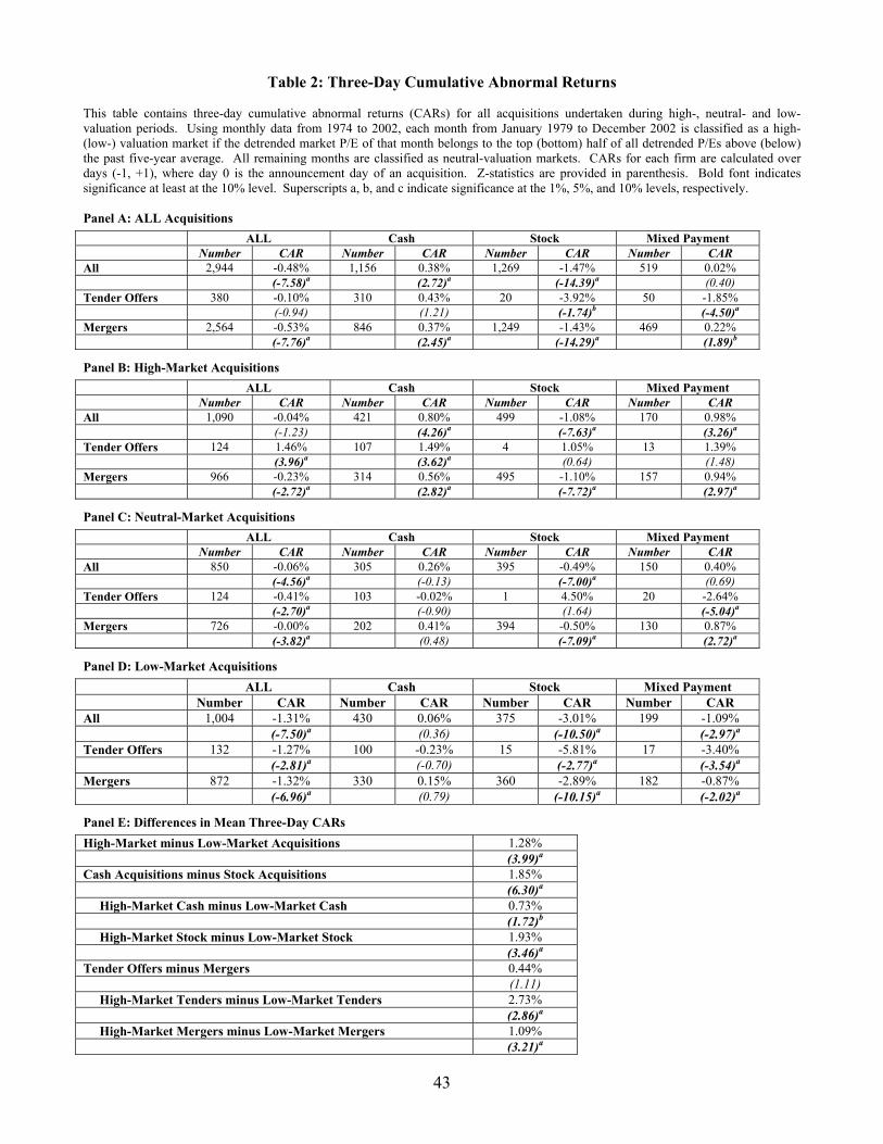
43

Table 2: Three-Day Cumulative Abnormal Returns This table contains three-day cumulative abnormal returns (CARs) for all acquisitions undertaken during high-, neutral- and low-valuation periods. Using monthly data from 1974 to 2002, each month from January 1979 to December 2002 is classified as a high- (low-) valuation market if the detrended market P/E of that month belongs to the top (bottom) half of all detrended P/Es above (below) the past five-year average. All remaining months are classified as neutral-valuation markets. CARs for each firm are calculated over days (-1, +1), where day 0 is the announcement day of an acquisition. Z-statistics are provided in parenthesis. Bold font indicates significance at least at the 10% level. Superscripts a, b, and c indicate significance at the 1%, 5%, and 10% levels, respectively. Panel A: ALL Acquisitions

ALL Cash Stock Mixed Payment Number CAR Number CAR Number CAR Number CAR

All 2,944 -0.48% 1,156 0.38% 1,269 -1.47% 519 0.02% (-7.58)a (2.72)a (-14.39)a (0.40) Tender Offers 380 -0.10% 310 0.43% 20 -3.92% 50 -1.85% (-0.94) (1.21) (-1.74)b (-4.50)a Mergers 2,564 -0.53% 846 0.37% 1,249 -1.43% 469 0.22% (-7.76)a (2.45)a (-14.29)a (1.89)b Panel B: High-Market Acquisitions

ALL Cash Stock Mixed Payment Number CAR Number CAR Number CAR Number CAR

All 1,090 -0.04% 421 0.80% 499 -1.08% 170 0.98% (-1.23) (4.26)a (-7.63)a (3.26)a Tender Offers 124 1.46% 107 1.49% 4 1.05% 13 1.39% (3.96)a (3.62)a (0.64) (1.48) Mergers 966 -0.23% 314 0.56% 495 -1.10% 157 0.94% (-2.72)a (2.82)a (-7.72)a (2.97)a Panel C: Neutral-Market Acquisitions

ALL Cash Stock Mixed Payment Number CAR Number CAR Number CAR Number CAR

All 850 -0.06% 305 0.26% 395 -0.49% 150 0.40% (-4.56)a (-0.13) (-7.00)a (0.69) Tender Offers 124 -0.41% 103 -0.02% 1 4.50% 20 -2.64% (-2.70)a (-0.90) (1.64) (-5.04)a Mergers 726 -0.00% 202 0.41% 394 -0.50% 130 0.87% (-3.82)a (0.48) (-7.09)a (2.72)a Panel D: Low-Market Acquisitions

ALL Cash Stock Mixed Payment Number CAR Number CAR Number CAR Number CAR

All 1,004 -1.31% 430 0.06% 375 -3.01% 199 -1.09% (-7.50)a (0.36) (-10.50)a (-2.97)a Tender Offers 132 -1.27% 100 -0.23% 15 -5.81% 17 -3.40% (-2.81)a (-0.70) (-2.77)a (-3.54)a Mergers 872 -1.32% 330 0.15% 360 -2.89% 182 -0.87% (-6.96)a (0.79) (-10.15)a (-2.02)a Panel E: Differences in Mean Three-Day CARs

High-Market minus Low-Market Acquisitions 1.28% (3.99)a Cash Acquisitions minus Stock Acquisitions 1.85% (6.30)a High-Market Cash minus Low-Market Cash 0.73% (1.72)b High-Market Stock minus Low-Market Stock 1.93% (3.46)a Tender Offers minus Mergers 0.44% (1.11) High-Market Tenders minus Low-Market Tenders 2.73% (2.86)a High-Market Mergers minus Low-Market Mergers 1.09% (3.21)a

44

Table 3: Two-Year Buy-and-Hold Abnormal Returns This table provides post-announcement buy-and-hold abnormal returns (BHARs) for all acquisitions undertaken during high-, neutral- and low-valuation markets. Using monthly data from 1974 to 2002, each month from January 1979 to December 2002 is classified as a high- (low-) valuation market if the detrended market P/E of that month belongs to the top (bottom) half of all detrended P/Es above (below) the past five-year average. All remaining months are classified as neutral-valuation markets. Skewness-adjusted t-statistics are provided in parenthesis. Bold font indicates significance at least at the 10% level. Superscripts a, b, and c indicate significance at the 1%, 5% and 10% levels, respectively. Significance is based on block-bootstrapped critical values. Panel A: ALL Acquisitions

ALL Cash Stock Mixed Payment Number BHAR Number BHAR Number BHAR Number BHAR

All 2,944 -7.22% 1,156 -0.55% 1,269 -13.19% 519 -7.46% (-5.16)a (-0.24) (-5.35)a (-2.85)a

Tender Offers 380 1.62% 310 2.17% 20 -24.48% 50 8.68% (0.49) (0.58) (-2.18)b (1.01)c

Mergers 2,564 -8.53% 846 -1.54% 1,249 -13.01% 469 -9.18% (-5.53)a (-0.60) (-5.23)a (-3.36)a

Panel B: High-Market Acquisitions

ALL Cash Stock Mixed Payment Number BHAR Number BHAR Number BHAR Number BHAR

All 1,090 -11.32% 421 -9.98% 499 -13.89% 170 -7.12% (-4.62)a (-2.85)a (-3.27)b (-1.66) Tender Offers 124 -5.13% 107 -7.47% 4 -31.64% 13 22.34% (-0.87) (-1.14) (1.48)c

Mergers 966 -12.12% 314 -10.83% 495 -13.75% 157 -9.55% (-4.52)a (-2.58)b (-3.21)b (2.15)b

Panel C: Neutral-Market Acquisitions

ALL Cash Stock Mixed Payment Number BHAR Number BHAR Number BHAR Number BHAR

All 850 -6.60% 305 4.95% 395 -16.33% 150 -4.46% (-2.99) (1.35)c (-6.01)a (-0.87) Tender Offers 124 11.52% 103 11.98% 1 -44.15% 20 11.93% (1.87)b (1.73)b (0.86) Mergers 726 -9.69% 202 1.36% 394 -16.26% 130 -6.98% (-4.33)b (0.34) (-5.97)a (-1.27)c

Panel D: Low-Market Acquisitions

ALL Cash Stock Mixed Payment Number BHAR Number BHAR Number BHAR Number BHAR

All 1,004 -3.28% 430 4.78% 375 -8.96% 199 10.01% (-1.34) (1.44) (-1.89) (-2.32)c

Tender Offers 132 -1.33% 100 2.38% 15 -21.26% 17 -5.59% (-0.22) (0.42) (-1.63) (-0.30) Mergers 872 -3.58% 330 5.51% 360 -8.45% 182 -10.42% (-1.32) (1.40) (-1.75) (-2.33)b

Panel E: Differences in Mean Two-Year BHARs

High-Market minus Low-Market Acquisitions -8.04% (2.60)a

Cash Acquisitions minus Stock Acquisitions -12.64% (-4.47)a

High-Market Cash minus Low-Market Cash -14.76% (-3.09)a

High-Market Stock minus Low-Market Stock -4.93% (-0.95) Tender Offers minus Mergers 10.15% (2.75)a

High-Market Tenders minus Low-Market Tenders -3.80% (-0.49) High-Market Mergers minus Low-Market Mergers -8.54% (-2.54)a

45

Table 4: Long-Run Stock Returns in Calendar Time Four-Factor Model Portfolio Regression Results

This table presents the results of four-factor portfolio regressions. Using monthly data from 1974 to 2002, each month from January 1979 to December 2002 is classified as a high- (low-) valuation market if the detrended market P/E of that month belongs to the top (bottom) half of all detrended P/Es above (below) the past five-year average. All other months are classified as neutral-valuation markets. For each month from 1982 to 2002 we form value-weighted portfolios of: (i) all sample firms that announced an acquisition in the previous two years (first column); (ii) sample firms that announced acquisitions during any high-valuation period within the previous two years (second column); and (iii) sample firms that announced acquisitions during any low-valuation period within the previous two years (third column). The portfolio excess returns are regressed on the Fama-French factors and the Carhart momentum factor as follows:

tppptftmpptftp eYRPRHMLhSMBsRRbaRR ,,,,, 1)( ++++−+=− The four factors are as follows: zero-investment portfolios representing excess return on the market, (Rm,t – Rf,t), the difference between a portfolio of “small” and “big” stocks, SMB, the difference between a portfolio of “high” and “low” book-to-market stocks, HML, and one-year momentum in stock returns as in Carhart (1997), PR1YR. Abnormal return is captured by the intercept of each regression. The fourth column presents a pooled portfolio regression:

tptftmppptftmpptftp eYRPRDHMLDSMBDRRDDYRPRmHMLhSMBsRRbaRR ,543,,21,,,, 1***)(*1)( ++++−+++++−+=− δδδδδ

where the dummy variable, D, equals one if the event portfolio return is a high-valuation return and zero otherwise. Difference in the performance of high and low-valuation acquirers is captured by the coefficient δ1. t-statistics are provided in parenthesis. Bold font indicates significance at least at the 10% level. Superscripts a, b, and c indicate significance at the 1%, 5% and 10% levels, respectively.

Full Sample Event Portfolio

High-Market Event Portfolio

Low-Market Event Portfolio

Pooled Portfolio

Estimate (t-value)

Estimate (t-value)

Estimate (t-value)

Estimate (t-value)

Intercept 0.66 0.68 1.35 1.35 (7.62)a (3.92)a (5.45)a (6.25)a

(Rmt –Rft) 1.02 1.06 1.07 1.07 (50.11)a (25.74)a (16.64)a (19.07)a

SMB -0.17 -0.09 -0.26 -0.26 (-6.44)a (-1.71)c (-3.83)a (-4.39)a

HML -0.15 -0.10 -0.41 -0.41 (-4.60)a (-1.60) (-4.83)a (-5.54)a

PR1YR -0.03 -0.06 -0.08 -0.08 (-1.86)c (-1.98)b (-2.04)b (-2.34)b

D -0.67 (-2.29)b

D * (Rmt –Rft) -0.01 (-0.15) D * SMB 0.17 (2.08)b

D * HML 0.31 (3.03)a

D * PR1YR 0.02 (0.32) Number of Observations 252 198 141 339 Adjusted R2 0.93 0.84 0.79 0.82

46

Table 5: Two-Year Abnormal Return on Operating Income

This table shows acquirers’ abnormal return on operating income (AROOI) averaged over the two years after the completion date for acquisitions undertaken during high-, neutral, and low-valuation markets. Using monthly data from 1974 to 2002, each month from January 1979 to December 2002 is classified as a high- (low-) valuation market if the detrended market P/E of that month belongs to the top (bottom) half of all detrended P/Es above (below) the past five-year average. Z-statistics for the medians are provided in parenthesis. The Z-statistics for the difference in medians in Panel E are based on the Wilcoxon-Mann-Whitney test and are shown in parenthesis. Bold font indicates significance at least at the 10% level. Superscripts a, b, and c indicate significance at the 1%, 5% and 10% levels, respectively.

Panel A: ALL Acquisitions

ALL Cash Stock Mixed Payment Number AROOI Number AROOI Number AROOI Number AROOI

All 2596 -1.19% 987 0.09% 1176 -2.76% 433 -0.95% (9.19)a (0.48) (12.42)a (2.74)a

Tender Offers 363 0.32% 299 0.32% 17 -0.54% 47 0.33% (1.10) (1.10) (0.24) (0.44) Mergers 2233 -1.42% 688 -0.02% 1159 -2.78% 386 -1.06% (10.35)a (0.15) (12.48)a (3.05)a

Panel B: High-Market Acquisitions

ALL Cash Stock Mixed Payment Number AROOI Number AROOI Number AROOI Number AROOI

All 932 -2.11% 327 -0.50% 472 -3.49% 133 -1.38% (8.91)a (1.16) (10.22)a (2.51)a

Tender Offers 119 -0.53% 104 -0.48% 3 -2.01% 12 -0.21% (0.83) (0.78) (0.00) Mergers 813 -2.40% 223 -0.50% 469 -3.50% 121 -1.41% (9.22)a (0.87) (10.20)a (2.64)a

Panel C: Neutral-Market Acquisitions

ALL Cash Stock Mixed Payment Number AROOI Number AROOI Number AROOI Number AROOI

All 785 -1.08% 284 0.49% 368 -2.32% 133 -1.38% (4.82)a (1.31) (7.30)a (1.47) Tender Offers 120 1.47% 99 1.42% 1 32.20% 20 0.31% (2.74)a (2.91)a (0.00) Mergers 665 -1.59% 185 -0.30% 367 -2.43% 113 -1.43% (6.40)a (0.51) (7.36)a (1.60)

Panel D: Low-Market Acquisitions

ALL Cash Stock Mixed Payment Number AROOI Number AROOI Number AROOI Number AROOI

All 879 -0.39% 376 0.19% 336 -1.34% 167 -0.38% (2.06)b (0.72) (3.49)a (0.85) Tender Offers 124 0.07% 96 -0.17% 13 -0.54% 15 1.44% (0.00) (0.20) (0.28) (0.77) Mergers 755 -0.41% 280 0.23% 323 -1.43% 152 -0.39% (2.22)b (0.96) (3.51)a (1.14)

Panel E: Differences in Median Two-Year AROOI

High-Market minus Low-Market Acquisitions -1.72% (-3.27)a

Cash Acquisitions minus Stock Acquisitions 2.85% (9.39)a

High-Market Cash minus Low-Market Cash -0.70% (-1.04) High-Market Stock minus Low-Market Stock -2.15% (-1.69)c

Tender Offers minus Mergers 1.74% (5.13)a

High-Market Tenders minus Low-Market Tenders -0.60% (-0.20)

High-Market Mergers minus Low-Market Mergers -1.98% (-3.28)a

47

Table 6: Regression Analysis of Short-Run and Long-Run Abnormal Returns This table contains ordinary least squares regressions of the acquirer’s three-day CARs (calculated using the CRSP equally-weighted index; results are similar when we use the value-weighted index instead), two-year BHARs, and two-year AROOI on the following variables. HighValMktDummy (NeutralValMktDummy) equals one if the month in which the acquisition was announced is classified as a high- (neutral-) valuation market and zero otherwise. Using monthly data from 1974 to 2002, each month from January 1979 to December 2002 is classified as a high- (low-) valuation market if the detrended market P/E of that month belongs to the top (bottom) half of all detrended P/Es above (below) the past five-year average. All other months are classified as neutral-valuation markets. CashDummy equals one if the total transaction value was paid in cash, non-convertible debt and/or non-convertible preferred stock and zero otherwise. MixedPaymentDummy equals one if the total transaction value was paid with a combination of cash and stock and zero otherwise. TenderDummye is one if the acquisition was a tender offer and zero otherwise. LogRelSize is the log of the transaction value at the time of the acquisition announcement divided by the acquirer’s market value of equity 30 days prior to the announcement. Acquirers are divided into equal subsamples of high, medium and low M/B firms based on their M/B ratio one month prior to the acquisition announcement. HighMBDummy (MediumMBDummy) equals one if the acquirer belongs to the high (medium) firm-valuation category. PoolingDummy equals one if the acquirer used pooling accounting and zero otherwise. PreAnnReturn is the firm’s average stock return measured over [-200,-31]. PaymentMethod consists of CashDummy and MixedPaymentDummy, which are as described above. StateOfMarket comprises HighValMktDummy and NeutralValMktDummy, which are also described above. Industry dummy variables correspond to the 17 Fama-French industry groupings. (Results are similar when we use one-digit or two-digit SIC codes instead.) In all panels, the intercept represents a low M/B, stock-financed merger that used purchase accounting and was announced in a low-valuation market. t-statistics are provided in parenthesis. Bold font indicates significance at least at the 10% level. Superscripts a, b, and c indicate significance at the 1%, 5%, and 10% levels, respectively.

Panel A: Dependent Variable

= three-day CAR

Panel B: Dependent Variable = two-year BHAR

Panel C: Dependent Variable = two-year AROOI

Estimate (t-value)

Estimate (t-value)

Estimate (t-value)

Intercept -4.80% -3.46% 0.65% (-1.27) (-0.10) (0.15) HighValMktDummy 3.17% -15.36% -1.80% (3.72)a (-1.97)b (-1.71)c NeutralValMktDummy 3.55% -18.02% -1.77% (4.27)a (-2.36)b (-1.73)c CashDummy 5.75% 30.15% 1.63% (7.11)a (4.08)a (1.58) MixedPaymentDummy 3.52% 12.02% 1.29% (3.95)a (1.48) (1.12) TenderDummy -1.05% -5.08% -0.29% (-1.12) (-0.59) (-0.25) LogRelSize -0.93% -0.97% 0.31% (-5.10)a (-0.59) (1.37) HighMBDummy 0.13% 0.22% 1.15% (0.27) (0.05) (2.35)b MediumMBDummy -0.03% 0.68% 1.93% (-0.08) (0.21) (4.50)a PoolingDummy -1.15% 13.19% 0.48% (-1.56) (1.94)b (0.52) PreAnnReturn 1.37% -22.31% (2.50)b (-4.43)a Interaction terms: LogRelSize * PaymentMethod Yes Yes Yes LogRelSize * TenderDummy Yes Yes Yes LogRelSize * StateOfMarket Yes Yes Yes LogRelSize * PoolingDummy Yes Yes Yes StateOfMarket * PaymentMethod Yes Yes Yes StateOfMarket * TenderDummy Yes Yes Yes Year Dummy Variables Yes Yes Yes Industry Dummy Variables Yes Yes No F-statistic 3.21 3.45 7.70 Adjusted R2 4.39% 4.84% 10.20%

48

Table 7: Long-Run Performance of Early and Late Movers In this table, we present long-run stock and operating performance results for early and late movers in high-market merger waves and in low-market phases. Panel A contains results based on average two-year buy-and-hold returns. Panel B contains calendar-time four-factor model portfolio regression results. Panel C shows results based on average two-year abnormal return on operating income. Using monthly data from 1974 to 2002, each month from January 1979 to December 2002 is classified as a high- (low-) valuation market if the detrended market P/E of that month belongs to the top (bottom) half of all detrended P/Es above (below) the past five-year average. Early movers are assumed to be the first 10%, 15% or 20% of acquirers in each high-market merger wave or low-market phase (i.e. consecutive periods of high or low market valuations). All remaining acquirers are classified as late acquirers. In Panel A, skewness-adjusted t-statistics are provided in parenthesis. Significance is based on block-bootstrapped critical values. In Panel B, t-statistics are provided in parenthesis. In Panel C, Z-statistics for the medians are provided in parenthesis. The Z-statistics for the difference in medians are based on the Wilcoxon-Mann-Whitney test and are shown in parenthesis. In all panels, bold font indicates significance at least at the 10% level. Superscripts a, b, and c indicate significance at the 1%, 5% and 10% levels respectively. Panel A: Two-Year BHARs of Early and Late Movers

A1: High-Market Merger Wave A2: Low-Market Phase The First x % of Acquirers Assumed to be

Early Movers Early Movers Late Movers Difference (Early-Late) Early Movers Late Movers Difference

(Early-Late) Number BHAR Number BHAR Number BHAR Number BHAR

10% 98 5.57% 928 -13.96% 19.53% 97 -5.78% 898 -3.60% -2.18% (0.82)c (-5.16)a (2.35)a (-0.40) (-1.51) (-0.19)

15% 151 -1.28% 875 -13.95% 12.68% 144 -6.50% 851 -3.36% -3.14% (-0.16) (-4.95)a (2.01)b (-0.67) (-1.36) (-0.39)

20% 202 -6.92% 824 -13.36% 6.44% 197 -3.52% 798 -3.88% 0.36% (-1.24) (-4.58)a (1.20) (-0.44) (-1.59) (0.05)

Panel B: Calendar-Time Four-Factor Model Portfolio Regressions

B1: High-Market Merger Wave B2: Low-Market Phase The First x % of Acquirers Assumed to be

Early Movers

Number

Coefficient on (Early-Late) Dummy: δ1

Number

Coefficient on (Early-Late) Dummy: δ1 10% 267 0.860 253 0.689

(1.84)c (1.09) 15% 264 0.932 253 0.779

(2.10)b (1.29) 20% 268 0.957 251 0.052

(1.99)b (0.10) Panel C: Two-Year AROOI of Early and Late Movers

C1: High-Market Merger Wave C2: Low-Market Phase The First x % of Acquirers Assumed to be

Early Movers Early Movers Late Movers Difference (Early-Late) Early Movers Late Movers Difference

(Early-Late) Number AROOI Number AROOI Number AROOI Number AROOI

10% 84 -1.44% 787 -2.41% 0.97% 83 -3.87% 787 -0.19% -3.69% (2.18)b (9.08)a (1.31) (3.18)a (1.10) (-3.53)a

15% 127 -1.60% 744 -2.44% 0.84% 127 -3.61% 743 0.06% -3.55% (2.92)a (8.87)a (1.53) (3.81)a (0.62) (-4.42)a

20% 171 -1.18% 700 -2.62% 1.44% 171 -3.40% 699 0.00% -3.40% (2.98)a (8.92)a (2.29)b (4.35)a (0.11) (-5.36)a

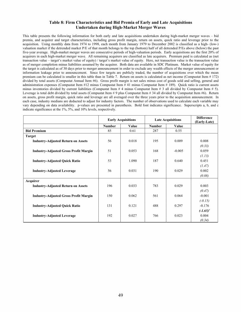
49

Table 8: Firm Characteristics and Bid Premia of Early and Late Acquisitions Undertaken during High-Market Merger Waves

This table presents the following information for both early and late acquisitions undertaken during high-market merger waves – bid premia, and acquirer and target characteristics, including gross profit margin, return on assets, quick ratio and leverage prior to the acquisition. Using monthly data from 1974 to 1998, each month from January 1979 to December 2002 is classified as a high- (low-) valuation market if the detrended market P/E of that month belongs to the top (bottom) half of all detrended P/Es above (below) the past five-year average. High-market merger waves are consecutive periods of high-valuation periods. Early acquisitions are the first 20% of acquirers in each high-market merger wave. All remaining acquirers are classified as late acquirers. Premium paid is calculated as (net transaction value – target’s market value of equity) / target’s market value of equity. Here, net transaction value is the transaction value as of merger completion minus liabilities assumed by the acquirer. Both data are available in SDC Platinum. Market value of equity for the target is calculated as of 30 days prior to merger announcement in order to exclude any wealth effects of the merger announcement or information leakage prior to announcement. Since few targets are publicly traded, the number of acquisitions over which the mean premium can be calculated is smaller in this table than in Table 7. Return on assets is calculated as net income (Compustat Item # 172) divided by total assets (Compustat Annual Item #6). Gross profit margin is net sales minus cost of goods sold and selling, general and administration expenses (Compustat Item #12 minus Compustat Item # 41 minus Compustat Item # 189). Quick ratio is current assets minus inventories divided by current liabilities (Compustat Item # 4 minus Compustat Item # 3 all divided by Compustat Item # 5). Leverage is total debt divided by total assets (Compustat Item # 9 plus Compustat Item # 34 all divided by Compustat Item #6). Return on assets, gross profit margin, quick ratio and leverage are all averaged over the three years prior to the acquisition announcement. In each case, industry medians are deducted to adjust for industry factors. The number of observations used to calculate each variable may vary depending on data availability. p-values are presented in parenthesis. Bold font indicates significance. Superscripts a, b, and c indicate significance at the 1%, 5%, and 10% levels, respectively.

Early Acquisitions Late Acquisitions Difference (Early-Late)

Number Value Number Value Bid Premium 85 0.61 287 0.55 Target Industry-Adjusted Return on Assets 56 0.018 195 0.009 0.008 (0.33) Industry-Adjusted Gross Profit Margin 51 0.053 168 -0.005 0.059 (1.13) Industry-Adjusted Quick Ratio 53 1.090 187 0.640 0.451 (1.47) Industry-Adjusted Leverage 56 0.031 190 0.029 0.002 (0.08) Acquirer Industry-Adjusted Return on Assets 196 0.033 783 0.029 0.003 (0.47) Industry-Adjusted Gross Profit Margin 150 0.062 561 0.064 -0.001 (-0.15) Industry-Adjusted Quick Ratio 131 0.121 488 0.297 -0.176 (-1.65)c Industry-Adjusted Leverage 192 0.027 766 0.023 0.004 (0.34)

50

Table 9: Effect of Firm Valuation In this table we examine the impact of market valuations by controlling for acquirer industry-adjusted M/B, which we define as the acquirer’s M/B ratio one month prior to the acquisition announcement normalized by the industry’s M/B ratio in that month, where industries are based on the 17 Fama-French industry groupings. (Results are similar if we use two-digit SIC codes; if we define industry-adjusted M/B as the acquirer’s M/B minus the industry’s M/B; or if we do not industry-adjust M/B ratios.) We split the sample into equal subsamples of high, medium and low (industry-adjusted) M/B acquirers, and examine the performance of acquirers buying during high- and low-valuation markets for each M/B category. Using monthly data from 1974 to 2002, each month from January 1979 to December 2002 is classified as a high- (low-) valuation market if the detrended market P/E of that month belongs to the top (bottom) half of all detrended P/Es above (below) the past five-year average. All other months are classified as neutral-valuation markets. Skewness-adjusted t-statistics are provided in parenthesis. Inference is based on block-bootstrapped t-statistics. Bold font indicates significance at least at the 10% level. Superscripts a, b and c indicate significance at the 1%, 5% and 10% levels respectively. Panel A: ALL Acquisitions Split by Acquirer Industry-Adjusted M/B ratios

High-Market Acquisitions Low-Market Acquisitions Number BHAR Number BHAR ALL 1090 -11.32% 1004 -3.28% (-4.63) a (-1.34) a High M/B 289 -11.72% 461 -7.62% (-1.72) a (-1.91) a

Medium M/B 363 -14.64% 320 -2.90% (-4.79) a (-0.94) a

Low M/B 438 -8.31% 223 5.13% (-3.17) a (0.93) b

Panel B: Differences in Mean Two-Year BHARs

High-Market minus Low-Market Acquisitions -8.04% (-2.60) a

High M/B: High-Market minus Low-Market -4.10% (-0.59) Medium M/B: High-Market minus Low-Market -11.74% (-2.87) a

Low M/B: High-Market minus Low-Market -13.44% (-2.02) b

51

Table 10: Alternative Specification of High- and Low-Valuation Periods This table presents differences in the performance of high- and low-market acquisitions using two-year BHARs (Panel A) and four-factor model portfolio regressions (Panel B). High- and low-valuation periods are identified using seven methods. Our base method is Method I (P/E Ratio, Monthly): Using monthly data from 1974 till 2002, each month from January 1979 till December 2002 is classified as a high- (low-) valuation market if the detrended market P/E of that month belongs to the top (bottom) half of all detrended P/Es above (below) the past five-year average. Method II (S&P Index Level) uses the detrended S&P index level instead of the detrended market P/E. Method III (P/E Ratio, Quarterly) uses quarterly instead of monthly P/E data. Method IV (P/E Ratio, Equal) imposes an equal number of high- and low-valuation periods by classifying a month as high (low) valuation if the detrended market P/E of that month belongs to the top (bottom) third of all detrended P/Es. Method V (P/E Ratio, Std. Dev.) classifies a month as high- (low-) valuation market if the detrended market P/E of that month is 0.5 standard deviations above (below) the mean detrended P/E during this period instead of classifying the top (bottom) half of all detrended P/Es above (below) the past five-year average as such. Method VI (M/B Ratio, Market) uses the M/B ratio of the overall market (defined as the median M/B ratio of all publicly-listed firms) instead of the P/E ratio of the S&P500. Method VII (M/B Ratio, Industry) uses the M/B ratio of the acquirer’s industry (defined as the median M/B ratio of all publicly-listed firms in that industry) instead of the P/E ratio of the S&P500. Industries correspond to the 17 Fama-French industry groupings. t-statistics are provided in parenthesis. Bold font indicates significance at least at the 10% level. Superscripts a, b, and c indicate significance at the 1%, 5% and 10% levels respectively. Panel A: Differences in the performance of high-market and low-market acquisitions using two-year BHARs

Method to Identify High- and Low-Valuation Periods ==>

I Base: P/E Ratio

(Monthly)

II S&P Index

Level

III P/E Ratio

(Quarterly)

IV P/E Ratio (Equal)

V P/E Ratio (Std. Dev.)

VI M/B ratio (Market)

VII M/B ratio (Industry)

High-Market minus Low-Market -8.04% -8.27% -8.62% -7.74% -7.33% -3.81% -9.70% (2.60)a (-2.79)a (-2.96)a (-2.53)a (-2.37)a (-1.09) (-3.12)a

Cash Acquisitions minus Stock Acquisitions -12.64% 12.64% 12.64% 12.64% 12.64% 12.64% 12.64% (-4.47)a (4.47)a (-4.47)a (4.47)a (-4.47)a (4.47)a (-4.47)a

High-Market Cash minus Low-Market Cash -14.76% -13.05% -14.64% -15.40% -15.70% -12.86% -1.31% (-3.09)a (-2.79)a (-3.07)a (-3.30)a (-3.09)a (-2.12)b (-0.23) High-Market Stock minus Low-Market Stock -4.93% -6.49% -6.11% -3.96% -3.31% 4.45% -17.30% (-0.95) (-1.34) (-1.40) (-0.78) (-0.71) (0.91) (-3.81)a

Tender Offers minus Mergers 10.15% 10.15% 10.15% 10.15% 10.15% 10.15% 10.15% (2.75)a (2.75)a (2.75)a (2.75)a (2.75)a (2.75)a (2.75)a

High-Market Tenders minus Low-Market Tenders -3.80% -5.60% -1.08% -6.93% -7.66% -10.71% 10.29% (-0.49) (-0.75) (-0.13) (-0.93) (-0.90) (-0.99) (1.02) High-Market Mergers minus Low-Market Mergers -8.54% -8.54% -9.75% -7.70% -7.28 -2.67% -11.25% (-2.54)a (-2.65)a (-3.11)a (-2.31)b (-2.20)b (0.72) (-3.39)a

Panel B: Differences in the Performance of High-Market and Low-market Acquisitions using Four-Factor Model Portfolio Regressions

Method to Identify High- and Low-Valuation Periods ==>

I Base: P/E Ratio

(Monthly)

II S&P Index

Level

III P/E Ratio

(Quarterly)

IV P/E Ratio (Equal)

V P/E Ratio (Std. Dev.)

VI M/B ratio (Market)

VII M/B ratio (Industry)

Coefficient on (Early – Late) Dummy: δ1 -0.669 -0.589 -0.547 -0.584 0.021 0.236 -0.904 (-2.29)b (-1.91)c (-1.73)c (-1.94)c (0.05) (0.69) (-2.87)a

52

Table 11: Price Reversals Two-year BHARs of Acquirers Split By Pre-event Performance

In this table we present pre-announcement buy-and-hold returns as well as two-year post-announcement buy-and-hold abnormal returns of six categories of acquirers. Acquirers are first divided into two groups – high-market acquirers and low-market acquirers. The former (latter) are acquirers who bought firms during periods of high (low) stock-market valuations. The classification of high- and low-valuation periods is done using our base P/E Ratio (Monthly) method (see below for a description). Both high-market and low-market acquirers are further subdivided into three categories: (i) acquirers whose six-month pre-announcement buy-and-hold returns belonged in the top quintile (ii) acquirers whose six-month pre-announcement buy-and-hold returns belonged in the bottom quintile, (iii) all remaining acquisitions. For buy-and-hold abnormal returns, skewness-adjusted t-statistics are provided in parenthesis. Inference is based on block-bootstrapped critical values. Bold font indicates significance at least at the 10% level. Superscripts a, b, and c indicate significance at the 1%, 5% and 10% levels respectively. P/E Ratio (Monthly): Using monthly data from 1974 to 2002, each month from January 1979 to December 2002 is classified as a high- (low-) valuation period if the detrended market P/E of that month belongs to the top (bottom) half of all detrended P/Es above (below) the past five-year average.

High-Market Acquirers Low-Market Acquirers

Top Quintile in Terms of Pre-Event Returns

Bottom Quintile in Terms of Pre-Event Returns

Remaining Top Quintile in Terms of Pre-Event Returns

Bottom Quintile in Terms of Pre-Event Returns

Remaining

Number of Firms 203 203 611 197 197 593 Average 6-Month Pre-Event Buy-and-Hold Return 87.67% -11.11% 17.99% 95.49% -19.06% 8.73% Average Two-Year Post-Event Buy-and-Hold Abnormal Return -14.67% -11.52% -12.45% -20.87% 6.86% -1.42% (-3.00)a (-2.23)c (-3.64)a (-3.41)b (1.09) (-0.51)

53

Table 12: Alternative Sample Periods: Difference in Two-Year BHARs for High- and Low-Market Acquisitions

This table presents the difference between the two-year buy-and-hold abnormal returns of acquisitions undertaken during high- and low-valuation periods for five alternative sample periods: 1979-1994, 1995-2002, 1979-1997, 1998-2002, and 1979-2002. The classification of high- and low-valuation periods is done using our base P/E Ratio (Monthly) method: each month is classified as a high- (low-) valuation market if the detrended market P/E of that month belongs to the top (bottom) half of all detrended P/Es above (below) the past five-year average. t-statistics are provided in parenthesis. Bold font indicates significance at least at the 10% level. Superscripts a, b, and c indicate significance at the 1%, 5% and 10% levels respectively. Significance is based on block-bootstrapped critical values.

Full sample 1979–1994 versus 1995–2002 1979–1997 versus 1998–2002 1979-2002 1979-1994 1995-2002 1979-1997 1998-2002

High-Market minus Low-Market -8.04% -8.97% -8.47% -15.82% -12.83% (2.60)a (-1.31) (-2.49)a (-2.60)a (-2.97)a

Cash Acquisitions minus Stock Acquisitions -12.64% -7.41% -13.04% -6.35% -17.57% (-4.47)a (-1.59) (-3.84)a (-1.68)c (-4.30)a

High-Market Cash minus Low-Market Cash -14.76% 1.61% -18.23% -10.52% -20.08% (-3.09)a (0.18) (-3.41)a (-1.34) (-3.14)a

High-Market Stock minus Low-Market Stock -4.93% -32.9% -2.30% -30.73% -6.07% (-0.95) (-2.29)b (-0.41) (-2.48)a (-0.83) Tender Offers minus Mergers 10.15% 14.40% 2.78% 14.72% 1.05% (2.75)a (2.37)a (0.62) (2.91)a (0.20) High-Market Tenders minus Low-Market Tenders -3.80% 16.54% -12.61 7.43% -31.61% (-0.49) (1.25) (-1.39) (0.65) (-3.18)a

High-Market Mergers minus Low-Market Mergers -8.54% -17.68% -7.96% -21.16% -11.01% (-2.54)a (-2.19)b (-2.18)b (-2.91)a (-2.35)a

54

Figure 1: Detrended Market P/E and Acquisitions Over Time This figure shows the detrended market P/E minus its five-year average, and acquisitions announced in high-valuation (=3), neutral-valuation (=2) and low-valuation (=1) markets over time.

-14

-12

-10

-8

-6

-4

-2

0

2

4

6

Jan-79 Jan-81 Jan-83 Jan-85 Jan-87 Jan-89 Jan-91 Jan-93 Jan-95 Jan-97 Jan-99 Jan-01

Detrended Market P/E minus Five-Year Average

High-Market (=3), Neutral-Market (=2) and Low-Market (=1) Acquisitions

55

Figure 2: Main results This figure summarizes our main results: although high-market acquisitions generate significantly higher announcement returns (CARs) for their shareholders than low-market acquisitions, their long-run stock performance (BHARs and calendar-time returns) and operating performance (AROOI) is significantly lower.

-18%-16%-14%-12%-10%-8%-6%-4%-2%0%2%

CARs BHARs CalendarTime AROOI