Market Structure, Liability, and Product Safety*

by

Andrew F. Daughety and Jennifer F. Reinganum** Department of Economics and Law School Vanderbilt University March 2016

* Prepared for inclusion in: Corchón, Luis C. and Marini, Marco A., Handbook of Game Theory and Industrial Organization, Edward Elgar, forthcoming. ** andrew.f.daughety@vanderbilt.edu; jennifer.f.reinganum@vanderbilt.edu

2

1 Introduction

In this chapter we consider how models of imperfect competition, developed by scholars working

in industrial organization (IO), provide insight into an important area of law: products liability (that is,

liability for harms and losses associated with goods and services sold via markets). This importance

derives from the fact that everyday life generally involves consumption activities wherein the risk of harm

is present: we all consume manufactured goods and commercially-harvested and/or prepared foods,

translocate or telecommute between home and employment, and occupy space in buildings and homes

that condition the air we breathe and the light we use (not to mention relying upon the safety of those

structures).

Remarkably, traditional law and economics (L&E) analyses of products liability generally find no

role for the influence of market structure or strategic interaction on liability policy. Two results come

from the traditional analysis. First, different liability regimes (to be detailed below) lead to the same

private choices of safety, and this private choice is the socially-optimal level of safety.1 Second,

alternative market structures (perfect competition, monopoly, oligopoly) have no effect on the level of

safety chosen by firms. In what follows, after briefly summarizing the traditional analysis, we consider

two simple (but plausible) model modifications that yield a substantial impact of market structure on the

choice of safety and (potentially) on the choice of liability regime. Section 2 provides a summary of the

traditional model used to consider unilateral precaution in the case of harms due to products; Section 3

then re-considers the traditional model of harm while Section 4 re-considers the traditional model of

production cost. In both Sections 3 and 4 we first consider monopoly provision of the product and then

extend the model to the case of oligopoly competition. Section 5 provides a brief review of additional

contributions to this literature and summary comments.

1 Formally, this statement assumes that precaution against an accident occurring is unilateral: only one agent’s choice of precaution

(usually taken to be the manufacturer of the product) affects the expected harm. We focus on the unilateral precaution case in this paper; for a discussion of the bilateral precaution case (i.e., wherein the consumer must also take care), see Shavell (1987) for the model in Section 2, and Daughety and Reinganum (2013b) for the model in Section 3.

3

2. The Traditional L&E Model of Products Liability under Unilateral Precaution2

2.1 Preliminaries: Consumers

A representative consumer has quasilinear utility for two goods, the product of interest

(consumed in an amount q > 0) and a “numeraire” good of amount z > 0; the consumer’s income is I and

the numeraire’s price will always be 1 while the price of the good of interest (abstracting from safety

considerations) is p > 0.3 Let U(q, z) = u(q) + z be the utility the consumer derives from consumption of

(q, z), again abstracting from any safety considerations associated with the good of interest. Let h(x) be

the expected harm (per unit of the good) that the consumer suffers when the firm supplying the product

has taken care level x. Finally, depending upon the liability regime in place, consumers who are harmed

may be compensated. Under strict liability, the consumer will be compensated by the firm for any harm

due to use of the product (that is, independent of the level of precaution the firm took) while under no

liability, the consumer is not compensated for harm by the firm.4 In what follows, let r denote the liability

regime and let δ be an indicator variable wherein δ = 1 if the liability regime is no liability (r = NL) while

δ = 0 if the liability regime is strict liability (r = SL). Thus, the consumer’s total utility from consuming

the bundle (q, z) is U(q, z; x, δr) = u(q) + z - δrh(x)q, for r = SL, NL.5

Assumption 1:

a) The direct utility for the good of interest, u(q), satisfies (for all q > 0):

1) u(q) > 0; 2) uʹ(q) > 0; and 3) uʺ(q) < 0.

b) Per-unit expected harm, h(x) satisfies (for all x > 0):

1) h(0) is positive and finite, and h(x) > 0 for all x > 0; 2) hʹ(x) < 0; and 3) hʺ(x) > 0.

c) The consumer’s maximum willingness to pay for a unit of the good exceeds the worst per-unit

2 A comprehensive discussion of the traditional model can be found in Shavell (1987). 3 In what follows, assume that income, I, is sufficiently large so that positive levels of both goods are consumed at optimality, and all

functions are continuously differentiable as many times as needed. 4 A third alternative liability regime is negligence, wherein sufficient investment in safety meets a “due care standard,” relieving the

firm of paying compensation, while insufficient investment implies “fault,” thereby requiring the firm to compensate the consumer. Thus, negligence is a hybrid of strict liability and no liability; we will address it later in this discussion. Under complete and perfect information, in the traditional model there would be no basis for a firm to take insufficient care, so it would never be found negligent (i.e., at fault). As will be discussed below, the modification of the model of harm to be discussed in Section 3 will actually predict that the firm may purposely violate the negligence standard, as it will prefer strict liability. For a recent discussion of these three liability regimes in the modeling context of products liability issues of manufacturing defects, design defects, and warning defects, see Daughety and Reinganum (2013a).

5 In what follows we focus on a complete and perfect information model, so as to direct attention to very basic changes in the analysis

4

expected harm: uʹ(0) > h(0).

Assumption 1(a) implies downward-sloping demand for the good of interest. Assumption 1(b) reflects

the traditional assumption about investment in safety by the firm: increased investment reduces the

expected harm, but there are diminishing returns to investment in safety with respect to reduction of the

expected harm. Assumption 1(c) bounds the expected cost of harm; we assume that we are considering

products that should not be removed from the market because they are inherently extremely dangerous or

socially unacceptable. This is reasonable in a complete and perfect information model, since otherwise

consumers could simply avoid the market.

Notice that since strict liability (δ = 0) is taken to imply perfect compensation of the consumer by

the firm, then the consumer ignores the total expected harm, h(x)q, when buying q units of the good,

whereas no liability means that the consumer will bear the entire cost of harm. To see this, solve the

consumer’s choice model, maxq,z U(q, z; x, δr) subject to pq + z < I, which yields the (inverse) demand

model for the good of interest:

pr(q; x) = max{uʹ(q) - δrh(x), 0}, for r = SL, NL. (1)

Under assumption 1(c), this means that the first term in brackets above is always positive for some (q, x)

combinations, in which case pr(q; x) = uʹ(q) - δrh(x). That is, pSL(q; x) = uʹ(q) > 0, and pNL(q; x) = uʹ(q) -

h(x) > 0. Given the earlier assumptions, this means that both demand functions are downward-sloping,

with pNL(q; x) downward-shifted from pSL(q).

2.2 Preliminaries: Firms

Production reflects constant unit costs of production (this assumption will be modified in Section

4), though the unit cost of production is an increasing convex function of the level of safety.

Assumption 2:

C(x, q) = c(x)q, with: 1) c(0) = 0 and c(x) > 0 for all x > 0; 2) cʹ(x) > 0 for all x > 0 and cʹ(0) = 0;

and 3) cʺ(x) > 0 for all x.

In the rest of the discussion of the traditional model we assume that the firm is a monopolist; Shavell

that arise from the assumptions made regarding harm and cost.

5

(1987, p. 65-66) provides a discussion of the perfectly-competitive case. Thus, the profit function for a

firm operating under liability regime r can be written as:

Πr(q, x) = pr(q, x)q - c(x)q - (1 - δr)h(x)q. (2)

That is, ΠSL(q, x) = uʹ(q)q - c(x)q - h(x)q, since under SL the firm fully compensates the consumer for any

harm, while under NL, ΠNL(q, x) = uʹ(q)q - h(x)q - c(x)q, since the consumer discounts the value of the

good by the expected cost of harm. Obviously, ΠSL(q, x) = ΠNL(q, x), for all x and q; that is, the

consumer’s willingness-to-pay fully reflects any anticipated uncompensated harm. Since second-order

conditions are met, then the following first-order conditions characterize the firm’s optimal choices in

regime r, denoted as (qr, xr):6

Πrx(qr, xr) = - (cʹ(xr) + hʹ(xr))qr = 0; (3)

Πrq(qr, xr) = pr(q; x) + pr

q(q; x)q - c(x) - (1 - δr)h(x)

= uʹ(qr) + uʺ(qr)qr - (c(xr) + h(xr)) = 0. (4)

The properties of u(q), c(x) and h(x) imply that qr > 0. Thus, from (3) one sees that xr minimizes c(x) +

h(x) and is independent of both the equilibrium level of output and the liability regime: xNL = xSL. Note

also that the simple (separable) structure of the first-order conditions (3) and (4) relies upon Assumption

2(a) (i.e., constant returns to scale in production of output) as well as the form of the expected harm

function.

2.3 Efficiency and Primary Results for the Traditional Model

Welfare, denoted as W(q, x), is given by:

W(q, x) = u(q) - c(x)q - h(x)q. (5)

Assumptions 1 and 2 imply that W(q, x) is strictly concave in (q, x). Assuming a finite optimum, denoted

as (qW, xW), the first-order conditions require that (qW, xW) satisfy the following:

Wx(qW, xW) = - (cʹ(xW) + hʹ(xW))qW = 0; (6)

Wq(qW, xW) = uʹ(qW) - (c(xW) + h(xW)) = 0. (7)

Again, the properties in Assumptions 1 and 2 imply that qW is positive and, through a comparison

6

between equations (4) and (7), the usual simple monopoly result obtains: qr < qW; that is, the monopolist

restricts output relative to the welfare-maximizing level.7 Notice also that equations (6) and (3) imply

that xNL = xSL = xW: the firm chooses the welfare-maximizing level of safety. Since pr(q; x) = uʹ(q) -

δrh(x), the separability in q and x means that prqx(q; x) = 0. The foregoing welfare result is simply a

reflection of the Spence (1975) condition concerning the under- or over-supply of quality; since the cross-

derivative of the demand function is zero, the monopolist will choose to supply the efficient level of

quality (here, safety). Again, from equation (6), this will be where the sum of the per-unit production cost

and the per-unit expected loss from harm is minimized.

Proposition 1 summarizes the relevant results from the traditional model.

Proposition 1: The traditional model (Assumptions 1 and 2) yields three results.

(a) Firms (whether perfectly competitive or a monopoly) always choose to provide the efficient

level of safety: xNL = xSL = xW. Thus, the choice of liability regime does not matter.

(b) Monopolists undersupply output, and this is unaffected by the liability regime chosen:

qNL = qSL < qW. Thus, market structure only affects the level of output provided.

These results are readily extended to the traditional Cournot oligopoly version of the foregoing analysis.

A qualifier for Proposition 1(a) is important to note. Since under no liability there will be no costs of

formally adjudicating a “wrong,” while under strict liability some such costs are bound to be incurred,

some scholars have argued that NL is socially preferred to SL.8 We abstract from this argument about

administrative costs in evaluating welfare.

A broad implication of the results from the traditional model is policy separability: antitrust and

competition policies can be formulated and implemented without regard to the choice of tort regime in

products liability: considerations of market performance are separable from considerations of product

6 In the sequel, a subscript on a multivariate function indicates differentiation, e.g., Πr

x(x, q) ≡ ∂Πr(x, q)/∂x. We use primes (ʹ and ʺ) for derivatives of single-variable functions.

7 If the firms are price takers, then as Shavell shows (1987, pp. 65-66), both the output level and the safety level are efficiently provided by a competitive industry.

8 For example, this is the underlying argument in Polinsky and Shavell (2010) for using NL in the case of mass-marketed products. Note that this argument relies strongly on the assumption that the choice of x by a firm (or firms) is perfectly observable to consumers, so that feedback via the market is effective. If x is unobservable, a firm under NL would pick a safety investment of zero and rational consumers should expect that xNL = 0.

7

performance. Alternatively put, agencies or courts charged with formulating or implementing laws

concerned with product market competition need not be particularly bothered with concerns about vertical

product quality issues such as product safety, and the reverse as well: assessment of whether an agent is

liable or culpable for harm does not require examination (by, say, a court) of the degree of

competitiveness (or lack thereof) of the market wherein a good or service was acquired. This suggests an

economy of governmental/judicial decision-making and it also suggests that the two areas of law can

develop independently.

3. Modifying the Traditional Model’s Representation of Harm: Cumulative Harm

In the traditional model outlined in Section 2, total expected harm accrues in proportion to the

quantity of the good consumed, so that marginal and average harm are the same. There is no obvious

physical basis for this assumption; it is simply particularly useful in providing results as outlined in

Section 2. In this Section we modify this assumption and find that the resulting analysis provides

significantly different results from those presented above.9 In particular, allowing for the model of total

expected harm to be nonlinear in the quantity of the good consumed means that the marginal and average

harm are generally not the same; this implies that the choice of liability regime matters, and that market

structure matters as well.

In DR2014 we provide a number of motivating examples from food safety, pharmaceuticals,

environmental safety, privacy (both on the internet and in the physical world), and the operation of

physical systems (i.e., wherein friction can have an effect on breakdown). In all of these examples, per-

unit expected harm can be viewed as increasing in the quantity of the good consumed, so that total

expected harm is actually convex in q. To capture this we modify Assumption 1 as follows.

Assumption 1ʹ:

a) The direct utility for the good of interest, u(q), satisfies (for all q > 0):

1) u(q) > 0; 2) uʹ(q) > 0; and 3) uʺ(q) < 0.

b) Total expected harm is modeled by the function H(x, q) which is thrice continuously

8

differentiable with the following properties:

1) H(0, x) = 0 for all x > 0; H(q, x) > 0 for all q > 0, and all x > 0;

2) Hx(q, x) < 0 and Hq(q, x) > 0 for all (q, x) > 0; Hx(0, x) = 0 for all x > 0;

3) H(q, x) is strictly convex in (q, x) > 0, with strictly negative off-diagonal terms;

4) Hqqx(q, x) < 0 for all (q, x) > 0.

c) All optimization problems have a unique interior optimum, and all the respective payoff

functions (W, ΠSL, and ΠNL) have second-order matrices that are negative definite in a

sufficiently large neighborhood of these optima.

Assumption 1ʹ(a) is the same as Assumption 1(a); the primary difference between Assumption 1ʹ and

Assumption 1 is in the total expected harm function, H(q, x), which in Section 2 is h(x)q. Assumption

1ʹ(b)(1) is parallel to Assumption 1(b). Assumptions 1ʹ(b)(2) and 1ʹ(b)(3) extend the convexity of h(x)q

used in Section 2 to now hold for both x and q in H(q, x); Hxx > 0 parallels hʺ(x) > 0 from Section 2, but

now we add Hqq > 0, which was absent from Section 2 (there Hqq = 0); intuitively, expected harm is

decreasing in x but increasing in q at an increasing rate. Due to the multivariate nature of how harm is

assumed to arise (i.e., both via the level of x and the level of q), we will need a further assumption about

the interaction of q and x. There are diminishing returns to investment in safety (Hxx > 0), but increasing

the investment in safety ameliorates the convexity of total expected harm in usage-level, which requires

that ∂Hqq/∂x < 0.10 A handy example, consistent with all of the above properties of H(q, x) is h(x)q2, with

h(x) as in Section 2. This example was explored in the main text and in Technical Appendix A of

DR2014; it was also exploited in the oligopoly discussion in Technical Appendix C of DR2014 and will

be employed later in this Section to review that oligopoly analysis.

3.1 Monopoly Provision of Safety when Harm is Cumulative

To provide the clearest insight, we again start with a monopolistic firm and derive an updated

9 The results in this Section draw heavily on Daughety and Reinganum (2014), hereafter denoted as DR2014, particularly Technical

Appendix B. To our knowledge, the first paper to formally allow for and model nonlinear (in q) expected harm is Marino (1988). 10 As is shown in the Technical Appendix for DR2014, Assumption 1ʹ(b)(4) is equivalent to Hxq(x, q) < Hx(x, q)/q for all (x, q) > 0.

Marino (1988) instead considers the case wherein Hxq(x, q) > Hx(x, q)/q for all (x, q) > 0; his focus is on “tolerance” wherein increased use of a good diminishes the rate of expected loss.

9

version of Proposition 1. In the subsequent subsection we proceed to consider the effect of allowing for

oligopolistic competition (which can take one of two forms, depending upon the degree of

interdependency of harm among the consumer’s purchases). In a manner similar to that in Section 2, the

(inverse) demand function for the good, conditional on the liability regime, is:

pr(q; x) = uʹ(q) - δrHq(q, x), for r = SL, NL, (8)

which is positive for the relevant ranges of q and x.

The convexity of H implies that the marginal expected harm exceeds the average expected harm:

Hq(q, x) > H(q, x)/q. (9)

Equation (9) is key to understanding why a model with cumulative harm changes the results from those of

the traditional model. To see this, we will specify the profit functions and first-order conditions for the

SL-firm (that is, the firm under a regime of strict liability), the NL-firm (similarly, the firm under a

regime of no liability), as well as the relevant welfare function and first-order conditions. Let a firm’s

profit under regime r again be denoted as Πr(q, x), where:

Πr(q, x) = pr(q, x)q - c(x)q - (1 - δr)H(q, x). (10)

Using equation (8), in the case of strict liability the SL-firm’s profit function (δSL = 0) becomes:

ΠSL(q, x) = uʹ(q)q - c(x)q - H(q, x), (11)

and the first-order conditions for the SL-firm become:

ΠSx

L(q, x) = - cʹ(x)q - Hx(q, x) = 0; (12)

ΠSq

L(q, x) = uʹ(q) + uʺ(q)q - c(x) - Hq(q, x) = 0. (13)

Again, using equation (8), in the case of no liability, the NL-firm’s profit function (δNL = 1) becomes:

ΠNL(q, x) = uʹ(q)q - c(x)q - Hq(q, x)q, (14)

and the first-order-conditions for the NL-firm become:

ΠNx

L(q, x) = - cʹ(x)q - Hqx(q, x)q = 0; (15)

ΠNq

L(q, x) = uʹ(q) + uʺ(q)q - c(x) - Hqq(q, x)q - Hq(q, x) = 0. (16)

Finally, welfare is as follows:

W(q, x) = u(q) - c(x)q - H(q, x), (17)

10

and the first-order-conditions for a maximum are the following:

Wx(q, x) = - cʹ(x)q - Hx(q, x) = 0; (18)

Wq(q, x) = uʹ(q) - c(x) - Hq(q, x) = 0. (19)

Some observations are now in order. First, as remarked upon earlier, the convexity of H in q

implies that Hq(q, x) > H(q, x)/q (the marginal expected harm due to increased consumption exceeds the

average expected harm), so comparing equations (11) and (14) provides the immediate result that for any

given relevant (q, x):

ΠNL(q, x) < ΠSL(q, x).

That is, for given (q, x), a firm will prefer a regime of strict liability to a regime of no liability; this

reflects the fact that while in the traditional model no liability results in a downward shift of the demand

curve from that under strict liability, under cumulative harm, no liability results in a rotation of the

demand curve. For example, if H(q, x) = h(x)q2, then demand under no liability becomes uʹ(q) - 2h(x)q

rather than what would obtain under strict liability: uʹ(q).

Second, for any given q, equations (12) and (18) yield the same value of x; that is, for a given

output level, a firm under the SL regime provides the welfare-maximizing level of safety; a comparison of

equations (15) and (18) show this does not hold for the NL regime. More precisely, let xSL(q) solve

equation (12), let xNL(q) solve equation (15), and let xW(q) solve equation (18). Then evaluating

equations (12) and (15) at xSL(q), and recalling the properties of H (see footnote 10) yields:

ΠNx

L(q, xSL(q)) = Hx(q, xSL(q)) - Hqx(q, xSL(q))q > 0,

meaning that at the given level of output, q, the NL-firm would choose a higher level of safety. That is:

xSL(q) = xW(q) < xNL(q).

All three functions are upward-sloping11 and equal zero when the quantity level is zero. We can think of

these as a type of (non-strategic) “best response” function, as they provide the optimal choice of the level

of safety investment for any exogenously specified level of quantity.

Let qSL(x) solve equation (13), let qNL(x) solve equation (16), and let qW(x) solve equation (19).

11

These functions provide (respectively) the SL-, NL-, and W-levels of optimal output for any arbitrary

given level of safety investment, x. In a manner similar to that used above, note that:

ΠNq

L(qSL(x), x) = - Hqq(qSL(x), x)qSL(x) < 0,

so that for any given x, qNL(x) < qSL(x). Similarly,

ΠSq

L(qW(x), x) = uʺ(qW(x))qW(x) < 0,

so the overall ordering for any given x is:

qW(x) > qSL(x) > qNL(x).

Let (x^ SL, q^ SL) simultaneously solve equations (12) and (13); then x^ SL = xSL(q^ SL) and q^ SL = qSL(x^ SL).

Similarly, let (x^ NL, q^ NL) simultaneously solve equations (15) and (16), so that x^ NL = xNL(q^ NL) and q^ NL =

qNL(x^ NL), and finally let (x^ W, q^ W) simultaneously solve equations (18) and (19), so x^ W = xW(q^ W) and q^ W =

qW(x^ W). In general qSL(x), qNL(x), and qW(x) are not monotonic, but one can show (see TAB2014) that

these functions are increasing up to, and beyond, where the related “best response” safety functions

(respectively xSL(q), xNL(q) , and xW(q)) cross the associated “best response” quantity functions, and that

these crossings are from below. Figure 1 illustrates the foregoing for the special case wherein H(q, x) =

h(x)q2, where h(x) is as in Section 2.

*** Place Figure 1 here ***

Two important lessons show up in Figure 1.12 First, the policies SL and NL provide very

different outcomes, in contrast with the traditional analysis from Section 2: market structure (as reflected

by the level of output) really does matter now. The NL safety curve is to the right of the SL curve, since

in order to reduce the effect on profits (which arises since the consumer discounts via the demand

function) the NL-firm increases x and simultaneously lowers q (which in turn means that the good’s price

is higher in the market than would otherwise occur). Second, if the liability regime is SL, then increases

in output brought about by, say, antitrust policy, result in (xSL(q), q) moving closer to (x^ W, q^ W), while

11 For this and other details, see the Technical Appendix, Part B, for DR2014; in the sequel, we refer to this as TAB2014. 12 Figure 1 shows the equilibrium safety level under NL as the same as the welfare-optimal level; this is a result of the quadratic form

employed, and is not a general property.

12

under an NL-policy, (xNL(q), q) diverges from (x^ W, q^ W).13 In other words, despite the interrelatedness of

the safety and quantity decisions, the policy-separability property we discussed in Section 2 as a valuable

result of the traditional model is available if agencies and courts involved in products liability tort actions

employ strict liability: product performance (i.e., concerns about the safety of products) is still separable

from market performance (i.e., concerns about the competitiveness of the marketplace), and decisions by

agencies and courts, as well as the development of law regarding these two spheres, can proceed

independently under SL.

One further point is worth making about how recognition of the non-proportionality of harm with

respect to consumption affects policy. Earlier we purposely chose to ignore negligence. Negligence is a

hybrid of SL and NL: a “due care” standard is set (perhaps at x^ W). A firm that chooses x below this

standard is fully liable for all harm while a firm that chooses x to be at least this great faces no liability.

Recall the result earlier that under cumulative harm, that ΠNL(q, x) < ΠSL(q, x) for any given (q, x). As we

show in DR2014, this preference for SL by the firm means that it has an incentive to undermine a regime

of negligence by purposely choosing x below the due-care standard if consumers observe the firm’s

choice of x prior to purchase (as has been assumed here). This would imply an SL-style market

exchange, which involves stronger product demand than would occur under compliance with a negligence

standard (resulting in NL).

3.2 Oligopolistic Provision of Safety when Harm is Cumulative

There are seemingly two means by which harm might accumulate via consumption of a collection

of products. On the one hand, consuming products from n firms, each of which independently creates

some harm which is (say) convex in the amount of the product consumed, may be viewed as creating

aggregate harm additively in the more-than-proportional consumption of each of the n products. In

DR2014 we refer to this as the “Diner’s Dilemma” by imagining the risks at an open buffet of dinner

items. One can get e coli from a portion of beef, or salmonella from a portion of chicken, or shigella

from a portion of vegetables. Upon becoming ill following dinner at the buffet, the particular source of

13 For the simple example wherein H(q, x) = h(x)q2, welfare is always higher under SL when compared with NL; in the more general

13

harm (the product) can be identified. On the other hand, bioaccumulation of mercury can come about

from consumption of a variety of mercury-containing fish.14 In this case the harm may be difficult to

associate with any one product or source: harm is convex in the aggregate exposure to mercury that

results from consumption of a variety of products.

3.2.1 Independent Cumulative Harm from n Products

To see the influence of market considerations, first consider the case wherein the consumer views

the n products as perfect substitutes in consumption (ignoring safety) and assume that product i’s

expected harm function is h(xi)(qi)2, i = 1, ..., n, wherein each h-function has the same properties as the h-

function in Section 2 (i.e., decreasing but convex in xi). Here we are assuming that harms are

independent and the source of a harm is identifiable. To facilitate providing clear results, assume that the

direct utility a consumer enjoys from consuming q = (q1, q2, ..., qn) of the n products is u(q) = αΣiqi -

(β/2)(Σiqi)2 where α and β are positive constants. Let Q = Σiqi, so the (inverse) demand for product i is α -

βQ when the liability regime is SL and α - βQ - 2h(xi)qi when the liability regime is NL. Therefore, under

SL, firm i’s profit function is ΠSLi (xi, qi; n) = (α - βQ)qi - h(xi)(qi)2 - c(xi)qi. We find the first-order

conditions for xi and qi, respectively, and then invoke symmetry, yielding:

- hʹ(x)q2 - cʹ(x)q = 0; (20)

α - (n + 1)βq - 2h(x)q - c(x) = 0. (21)

Simultaneous solution of equations (20) and (21) yields the symmetric Cournot-Nash equilibrium

combination of care and output, denoted x^ SL(n) and q^ SL(n), respectively.

Similarly, an NL-firm i’s profit function is ΠNLi (xi, qi; n) = (α - βQ - 2h(xi)qi)qi - c(xi)qi. We find

the first-order conditions for xi and qi, respectively, and then invoke symmetry, yielding:

-2hʹ(x)q2 - cʹ(x)q = 0; (22)

α - (n + 1)βq - 4h(x)q - c(x) = 0. (23)

Simultaneous solution of equations (22) and (23) yields the symmetric Cournot-Nash equilibrium

H(q, x) case, this will be true in a small enough neighborhood of (x^ W, q^ W).

14 Th U.S. F.D.A provides a strong warning, especially for pregnant women, nursing women, and young children, concerning the consumption of the following types of fish: shark, swordfish, king mackerel, and tilefish, alone or in combination. See

14

combination of care and output, denoted x^ NL(n) and q^ NL(n), respectively.

Finally, welfare when the consumption vector is q and the safety vector is x = (x1, x2, ..., xn) is:

W(q, x) = αΣiqi - (β/2)(Σiqi)2 - Σih(xi)(qi)2 - Σic(xi)qi.

Differentiating to obtain the first-order conditions and then applying symmetry provide the following

conditions for a welfare maximum:

Wx = -nhʹ(x)q2 - ncʹ(x)q = 0; (24)

Wq = nα - βn2q - 2nh(x)q - nc(x) = 0. (25)

Let the solution to equation (20) be denoted as xSL(q; n), and let the solution to equation (24) be denoted

as xW(q; n). Comparing equations (20) and (24) shows that:

xSL(q; n) = xW(q; n).

Moreover, modifying u(q) and H(q; x) to fit the current example, and comparing equation (12) with

equation (20) and equation (24) with equation (18), shows that:

xSL(q; n) = xW(q; n) = xSL(q) = xW(q),

so that, for any given level of output q, the SL-firm will choose the same level of safety for a given q

independent of the number of firms, and this will always be the socially optimal safety choice for that

level of output. Not surprisingly, xNL(q; n) is also independent of n and maintains the same relationship

with xW(q) as it held in the monopoly analysis. However, the number of firms does affect the (symmetric)

equilibrium quantity levels under SL, NL, or welfare maximization as specified in equations (21), (23),

and (25), respectively; in DR2014 we show how the fact that firms undersupply output affects the

equilibrium supply of safety (now no longer conditional on output level). In particular, we show that, as a

function of the number of firms and computed at the equilibrium oligopoly output in each case, SL-firms

undersupply safety while NL-firms oversupply safety (i.e., x^ SL(n) < x^ W(n) < x^ NL(n)). Under SL, NL, and

W, as the number of firms increases, each firm takes less care and produces a lower level of output, but

total output increases and risks are increasingly diversified over a larger set of firms from which to

purchase products.

http://www.fda.gov/food/resourcesforyou/consumers/ucm110591.htm, accessed March 18, 2016.

15

3.2.2 Interdependent Cumulative Harm from n Products

As pointed out earlier, the consumption of goods from different firms could lead to an overall

accumulation of harm because the alternative goods each contribute to the extent of exposure to the same

source of harm and it is the overall level of exposure that matters. A straightforward example is that

provided earlier: consumption of different types of fish, all of which contain mercury. If the expected

harm depends upon the aggregate level of exposure from all the goods, then the aggregate effect now is

(potentially) cumulative. Thus, let μ(xi) denote the amount of exposure per unit of good i consumed,

where μ(xi) has the same properties as h(xi) (that is, μ(0) is positive and finite, μʹ(x) < 0, and μʺ(x) > 0 for all x),

so that μ(xi)qi represents the amount of exposure from consuming qi units of product i. Thus, the

aggregate amount of exposure is Σiμ(xi)qi. We assume the expected harm is convex in the aggregate level

of exposure; in DR2014 we consider the simple quadratic form of this:

(Σiμ(xi)qi)2. (26)

Notice the contrast between this version of harm and that of the previous independent-harm model:

Σih(xi)(qi)2.

Space limitations prevent us from providing details of the analysis of this second model, but in

DR2014 we show that, in contrast with the independent harms model, the total expected harm arising

under an interdependent-harm process stays constant as n increases, so the risk of harm is not diversified

as n increases. Thus, for example, if there are fixed costs of production, this means that society is better

off restricting entry to one firm and regulating the product’s price, or subsidizing production, to increase

quantity. Second, unlike our results earlier, no standard liability regime provides the incentive to take the

socially-optimal level of care for a given level of output.

However, using our specific model of harm in equation (26), a simple multiplier in the firm’s

accounting for the expected harm, along with the use of exposure-based market-share liability (i.e.,

liability in proportion to μ(xi)qi/Σjμ(xj)qj), will make an SL-firm choose the socially-optimal level of

safety for a given output level. The multiplier is [2n/(n + 1)], so that firm i’s profit function under SL

16

incorporates this multiplier times the firm’s share of the exposure it contributes, times the total expected

harm:

(α - βQ)qi - [(2n/(n + 1)){μ(xi)qi/Σjμ(xj)qj}]{Σjμ(xj)qj}2 - c(xi)qi. (27)

Note that the firm bears additional liability (since 1 < 2n/(n + 1) < 2); the extra liability payment should

go to the state and not be part of compensation paid to harmed consumers. As shown in DR2014, this

allocation of liability induces each SL-firm’s choice of safety to be the same as that which a central

planner would choose (for a given output level).15

4. Modifying the Traditional Model’s Production Cost: Sequential Choice of Safety and Output

Another significant deviation from the basic products liability model involves a modification of

how choices about investment in safety affect the cost function. In particular, many products with a

safety attribute require up-front investment in R&D and product design. For example, investment in the

development of airbags for automobiles must occur before any airbags are installed in automobiles and

before those autos are subsequently sold. Investment in the development of pharmaceuticals must be

done, including testing for safety and effectiveness, before any of the product reaches the market. Thus,

safety involves an endogenously-determined fixed cost of development; it is also likely to impact the

variable cost of production. Typically, we view such a fixed investment as a long-run choice whereas

output can be varied in the short run. This suggests that firms’ product design investments (which

determine the safety of their products) should be viewed as being chosen in a prior period, with firms’

output choices being made in subsequent periods. Since the safety levels are long-lived, it is also

plausible to view them as being observed by all firms before output levels are chosen.

In Daughety and Reinganum (2006; hereafter DR2006), we provide a model wherein a number of

firms compete noncooperatively in a market for a product with safety attributes. In the first period, firms

make investments in product design; a higher investment implies a safer product, but a safer product also

has a higher marginal cost of production. Firms then observe the safety level of competitors’ products

15 Market share allocations of harm have been used by courts to allocate liability across firms in an industry when the source of the

harm (that is, which firm produced the product that caused a harm) was unclear; the most famous such case was Sindell v. Abbott Laboratories, 26 Cal. 3d 588 (1980).

17

(or, equivalently, they observe rival firms’ fixed investment and can infer the implied safety level), and

choose how much output to produce. Firms’ products have some inherent level of horizontal

differentiation, and they have at least the potential for vertical differentiation, since firms can choose any

level of safety. Because the products are differentiated and consumers value variety, we model this as N

identical consumers consuming some of each good. Consumption results in some accidents and harm to

consumers. Although we will assume that firms are strictly liable for the harm their products cause, we

also assume that the compensation process is imperfect so that consumers are left with some

uncompensated harm.16 This could reflect tort reforms such as a cap on non-economic damages or the

presence of litigation costs.17 As a consequence, a consumer’s willingness to pay for a product will be

sensitive to the product’s safety level, as the consumer will anticipate having to bear some uncompensated

loss should the product cause harm.

Some of the details of the DR2006 model will be simplified or suppressed here; see that paper for

a full development and discussion of the model. We will use the following notation:

n the number of firms, each of which produces a variety of the good; the n+1st good is a numeraire.

N the number of identical consumers in the market.

xi firm i’s safety level.

qi firm i’s output level per consumer; thus, firm i’s total output is Nqi.

t the unit cost of safety; thus, firm i’s total investment in safety is txi.

m(xi) the marginal cost of output for firm i; thus, firm i’s variable cost of providing qi units is m(xi)qi.

vc(xi) the portion of the expected harm borne by the consumer.

vf(xi) the portion of the expected harm borne by the firm.

We maintain the following assumptions about the functions m(xi) and the total expected harm

vc(xi) + vf(xi). The marginal cost of production, m(xi), is strictly positive, strictly increasing, and strictly

16 For simplicity, we will abstract from other issues that can introduce inefficiency. For example, we abstract from asymmetric

information about the level of harm, which can result in negotiation failure and expenditure on litigation; we also abstract from externalities in the sense of harm caused to third parties. These issues are considered in DR2006, and the interested reader is referred to that paper for the details.

17 Even if a case settles in pretrial negotiation (so no actual litigation costs are spent), if the firm has substantial bargaining power then the consumer’s settlement may not fully-compensate her. For example, in the extreme case wherein the firm makes a take-it-or-leave-it offer, the settlement offer would equal the consumer’s harm minus the costs she would incur by rejecting the offer and taking the case to trial.

18

convex in safety level. That is, marginal cost is constant with respect to output, but a safer product is

more costly to produce. The total expected harm, vc(xi) + vf(xi), encompasses multiple effects of safety.

It reflects the probability of an accident; the extent of harm conditional on the occurrence of an accident;

and any other costs such as litigation costs. Both the probability of an accident and the extent of harm

conditional on the occurrence of an accident may be affected by the safety level. We assume that the total

expected harm is strictly positive, strictly decreasing, and strictly convex. We revert here to the

assumption that expected harm is proportional to the level of consumption (as in the base model in

Section 2, and in contrast to the model with cumulative harm in Section 3), but we assume that safer

products generate lower expected harm.

We assume that each consumer has a quasilinear utility function, U(q, z), where q is again the n-

vector of quantities consumed and z is the numeraire good, so that:

U(q, z) = Σi αqi - (1/2)[Σi β(qi)2 + Σi Σj≠i γqiqj] + z. (28)

The parameters α, β, and γ are positive, with γ ≤ β. That is, products 1 through n are imperfect

substitutes. The parameter γ represents the extent of horizontal product differentiation; as γ converges to

β, the products become perfect substitutes (in terms of horizontal differentiation).

There are two ways to incorporate the consumer’s expected uncompensated harm, vc(xi). Given

that it is assumed to reflect a constant risk per unit of the good consumed, one way is to view it as a

reduction in utility. In this interpretation, we would substitute the expression α - vc(xi) for the parameter α

in the utility function. Alternatively, we could view this expected loss in dollar terms and incorporate it

into the consumer’s budget constraint. Letting I denote the consumer’s income, budget balance requires

that Σi[(pi + vc(xi))qi] + z = I. Either of these interpretations results in the same formal optimization

problem for the consumer.

maxq Σi αqi - (1/2)[Σi β(qi)2 + Σi Σj≠i γqiqj] + I - Σi [(pi + vc(xi))qi].

The resulting inverse demand function for product i is given by:

pi(q; xi) = α - vc(xi) - βqi - Σj≠i γqj. (29)

Firm i’s profit function is then given by:

19

πi(q; xi) = Nqi[pi(q; xi) - m(xi) - vf(xi)] - txi.

That is, firm i sells Nqi units overall, and makes a profit of pi(q; xi) - m(xi) - vf(xi) on each unit. The

safety investment, txi, increases with the safety level xi, but it does not vary with output. Upon

substituting for the function pi(q; xi) and collecting terms, we can re-write firm i’s profit as:

πi(q; xi) = Nqi[α - βqi - Σj≠i γqj - FMC(xi)] - txi, (30)

where “full marginal cost” FMC(xi) = m(xi) + vc(xi) + vf(xi). That is, although the expected losses from

harm are nominally shared by the consumer and the firm in the amounts of vc(xi) and vf(xi), respectively,

the consumer simply reduces her willingness to pay for product i by the amount of her expected

uncompensated harm as shown in equation (29). Thus, the firm faces the full marginal cost (that is, the

marginal production cost and the entire expected loss from accidents per unit of output).

In addition to the previous assumptions we made regarding the individual functions m(xi), vc(xi),

and vf(xi), we further assume that FMC(xi) is convex and “U-shaped” so there is a safety level that

minimizes full marginal cost. Denote this safety level by x‾; this is the level of safety that would be

chosen in the traditional law and economics model of product safety wherein there is no endogenous fixed

cost reflecting, say, safety design (i.e., wherein t = 0). It will become clear in what follows that a firm’s

safety level will always be less than x‾. Finally, we assume that FMC(0) < α (so the product can always be

produced profitably).

We will use first-order conditions to characterize the firms’ equilibrium output and safety levels.

Conditional on the vector of safety levels, the firms’ profit functions are strictly concave in their

respective output levels and the subgame perfect equilibrium in output levels can be computed directly.

Stepping back to the simultaneous choice of safety levels, this concavity is no longer guaranteed.

Nevertheless, we will assume that the reduced-form profit functions (as a function of the vector of safety

levels, taking into account how these affect the subgame perfect output levels) are strictly concave in the

firms’ respective safety levels and that the overall (symmetric) equilibrium is characterized by the first-

order conditions. We will use superscripts to indicate the number of firms; for instance, x1 and q1 will

20

denote a monopolist’s profit-maximizing choice of safety and output.

For the case of monopoly, π(q; x) = Nq[α - βq - FMC(x)] - tx. The profit-maximizing output

level, conditional on the safety level x, is q1(x) = (α - FMC(x))/2β. Substituting this into the profit

function yields the reduced-form profit as a function of safety level: Π(x) = N(α - FMC(x))2/4β - tx.

Thus, the monopolist’s profit-maximizing choice of safety level is given by:

(N/2β)[α - FMC(x1)][ - FMCʹ(x1)] - t = 0,

or, equivalently:

- Nq1(x1)FMCʹ(x1) - t = 0. (31)

It is clear that x1 < x‾; that is, because the unit cost of safety t is positive, the firm will choose a safety level

less than that which minimizes its full marginal cost (and therefore FMCʹ(x1) < 0). It is straightforward to

demonstrate the following comparative statics results. The monopolist’s safety level x1 (and output level

q1) increases with an increase in α or N, both of which generate an increase in the size of the market for

the product (a higher α reflects an increase in an individual consumer’s willingness to pay for the product

and a higher N reflects a larger number of consumers). The monopolist’s safety level x1 (and output level

q1) decreases with an increase in t (the unit cost of safety) or β (the rate at which a consumer’s willingness

to pay for the product declines with the quantity consumed).

Now we consider the oligopoly version of the model wherein n firms first noncooperatively

choose safety levels and subsequently, having observed rival safety levels, the n firms noncooperatively

choose output. The profit function has been provided above in equation (30). The first-order condition

for firm i’s choice of output is:

α - 2βqi - Σj≠i γqj - FMC(xi) = 0.

Solving the collection of first-order conditions for the subgame perfect vector of output level choices

(conditional on the vector of safety level choices, denoted x) yields:

qni(x) = [(2β - γ)α - (2β + (n - 2)γ)FMC(xi) + γΣj≠i FMC(xj)]/[(2β - γ)(2β + (n - 1)γ]. (32)

It is clear that each firm’s output level is increasing in its own safety level and decreasing in its rivals’

safety levels.

21

Now consider firm i’s choice of safety level, anticipating how it will affect all firms’ subgame

perfect choices of output. The first-order condition for xi is given by:

{- Nqni(x)FMCʹ(xi) - t} + Nqn

i(x)γΣj≠i [ - ∂qnj(x)/∂xi] = 0. (33)

The term in brackets is similar to that in equation (31) and represents the simple tradeoff between a higher

fixed cost of safety and a lower full marginal cost of output. The second term is positive since ∂qnj(x)/∂xi

= γFMCʹ(xi)]/[(2β - γ)(2β + (n - 1)γ] < 0. An increase in firm i’s safety level reduces its rivals’ subgame

perfect output levels, which translates into a higher inverse demand curve for firm i. This “business-

stealing” effect, which is absent from the monopoly model, provides an additional marginal benefit from

raising one’s safety level.

In what follows, we denote the symmetric equilibrium safety level for an n-firm oligopoly by xn,

and we denote the symmetric equilibrium output level for an n-firm oligopoly by qn. Under symmetry,

equations (32) and (33) become:

qn(xn) = [α - FMC(xn)]/[2β + (n - 1)γ]; (34)

- Nqn(xn)FMCʹ(xn){1 + γ2(n - 1)/[(2β - γ)(2β + (n - 1)γ]} - t = 0. (35)

The comparative statics results that were derived earlier in the monopoly case extend to the case

of oligopoly: the safety level xn (and output level qn) increases with an increase in α or N, and decreases

with an increase in t or β. However, now two additional parameters appear in the model. Both n and γ

are measures of market competitiveness; clearly a higher number of competitors (n) makes competition

more intense, but so does a greater degree of substitution (γ).

An increase in the number of firms results in a lower equilibrium safety level xn and output level

qn. The intuition for this is that, all else equal, more firms in the market will lead to a higher overall

output but a lower output per firm. A firm that anticipates a lower output will find it optimal to choose a

lower safety investment; although this investment lowers full marginal cost, this cost-reduction applies to

fewer units of output. Thus the return to investment in safety is lower when the number of firms is

higher.

∈An increase in the degree of substitution has more complex effects. Recall that γ [0, β]. When

22

γ = 0 each firm is a monopolist, whereas when γ = β the products are perfect substitutes. In general, the

degree of horizontal differentiation has a direct effect on the consumer’s marginal willingness to pay for

each good (a higher value of γ means a lower marginal willingness to pay for good i) and it has an

indirect effect on how responsive firm j’s output level is to the safety level of good i (a higher value of γ

makes business-stealing more effective). When γ is relatively small the business-stealing effect of an

increase in firm i’s safety level on firm j’s output is also relatively small as the products are poor

substitutes. Thus the overall effect is that xn decreases as γ increases, when γ is small. But when γ is

sufficiently large, then the indirect (business-stealing) effect dominates the direct effect (that is, the

reduced marginal willingness to pay for any one variety of the product) and xn increases as γ increases.

More formally, there is a threshold value γmin ∈(β, n) (0, β) such that xn decreases as γ increases for γ <

γmin(β, n) and xn increases as γ increases for γ > γmin(β, n). Moreover, it can be shown that γmin(β, n) is

increasing in n and that lim n→∞ γmin(β, n) = β. The impact of increasing γ on qn is also complex; it can be

shown that qn decreases as γ increases for γ < γmin(β, n), but the effect of further increases in γ is

ambiguous.

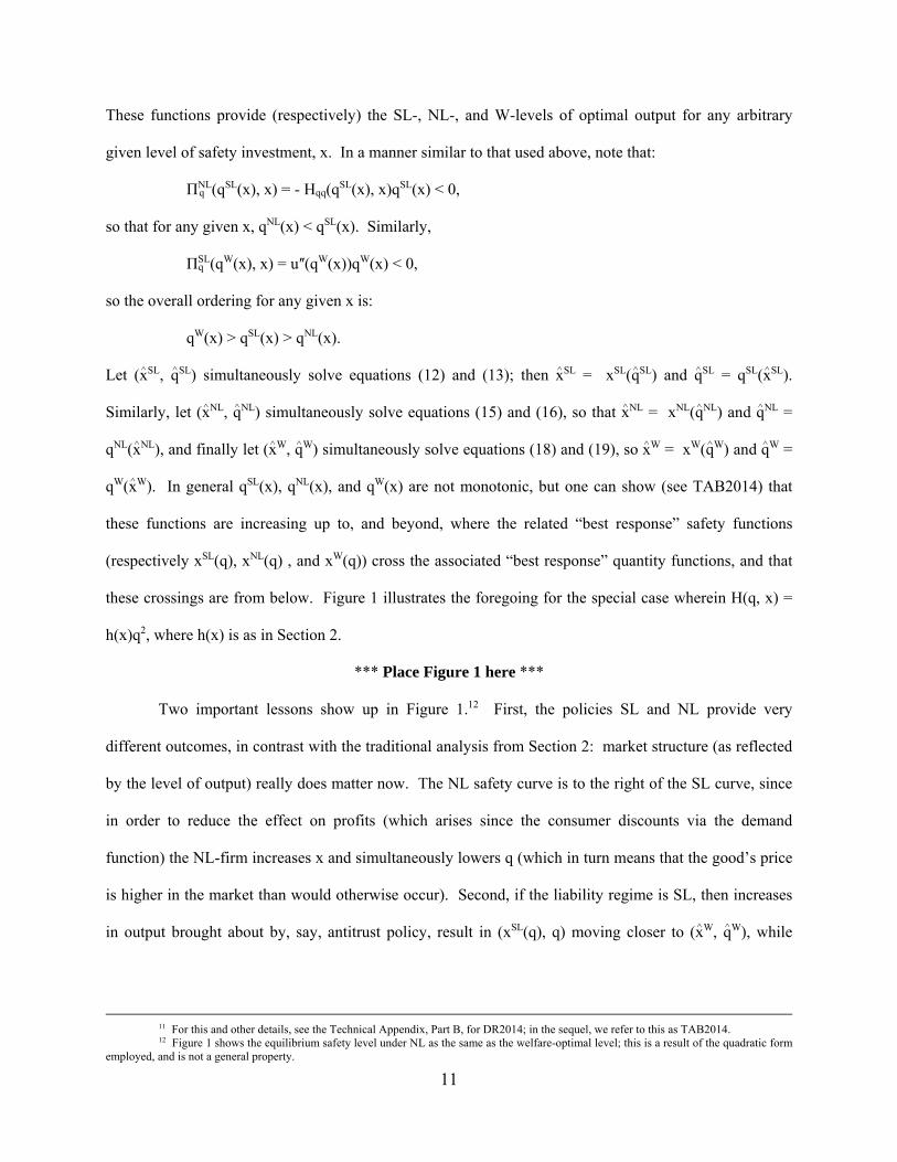
The dashed curves in Figure 2 illustrate the effects of increasing market competitiveness through

either increasing n or increasing γ. The extent of horizontal product differentiation (γ) is measured along

the horizontal axis. The equilibrium safety level (xn) is measured along the vertical axis. For n = 1 (or for

any n, if γ = 0), there is a single value of the safety level, denoted x1; this is less than x‾ , which is the safety

level at which FMC is minimized. For any particular n > 1, the equilibrium safety level first falls as γ

increases, but then rises once γ exceeds γmin(β, n). As n increases, each curve depicting xn is everywhere

below those for smaller values of n (except that they start at the same point, x1).

*** Place Figure 2 here ***

We now consider how a social planner that is interested in promoting socially-optimal safety

might behave. However, we will not consider an all-powerful social planner (that could, in principle,

choose the number of firms, the safety levels, and the output levels). Rather, our social planner will take

the number of firms and their non-cooperative behavior with respect to output choices as given. Under

23

these circumstances, what safety level would the social planner choose? If this is different from what the

firms themselves would choose in equilibrium, can the liability system be modified or augmented with

other policies to achieve the desired safety level?

Given a common safety level, denoted X (which will be chosen by the planner), the market

operates as before. Consumers determine their willingness to pay for the products and the firms non-

cooperatively choose their output levels. This generates utility for consumers, which our planner takes

into account, and production and expected liability costs for the firms, which our planner also takes into

account. Since our planner takes n as given and firms noncooperatively choose their output levels,

subgame perfect equilibrium output will be given by the same function as before. That is,

qn(X) = [α - FMC(X)]/[2β + (n - 1)γ]. (36)

The planner’s problem is then to choose X to maximize:

NU(q1 = ... = qn = qn(X)) - n[FMC(X)Nqn(X) + tX]. (37)

Let Xnq denote the planner’s optimal choice of safety level (we use the superscript “nq” to indicate that

the number of firms and the noncooperatively-chosen output levels are taken as given by the planner).

The resulting first-order condition is:

- Nqn(Xnq)FMCʹ(Xnq){(3β + (n - 1)γ)/(2β + (n - 1)γ)} - t = 0. (38)

Since the firms choose output noncooperatively in both scenarios, these are only different to the

extent that the social planner’s safety level (Xnq) is different from the noncooperative safety level (xn).

The comparative statics effects of Xnq with respect to increases in n, N, α, and β are the same as those of

xn. However, whereas xn was first decreasing and then increasing with an increase in γ, the social

planner’s safety level Xnq always decreases with an increase in γ. This is because there is no social return

to business-stealing. Indeed, it can be shown that there exists a threshold value Γnq ∈(β, n) (0, β] such

that noncooperative firms would choose a lower safety level than the planner for γ < Γnq(β, n), and a

higher safety level than the planner for γ > Γnq(β, n). For n = 2, it turns out that Γnq(β, n) = β; however,

since Γnq(β, n) decreases as n increases, it follows that Γnq(β, n) < β for n > 2.

The solid curves in Figure 2 illustrate the effects on Xnq of increasing market competitiveness

24

through either increasing n or increasing γ. Increasing either measure of competitiveness (holding the

other one fixed) results in a lower value of Xnq. Furthermore, the Figure illustrates the result that when

competition is sufficiently intense due to a substantial number of firms and/or a high degree of

substitution, the noncooperative firms’ equilibrium safety level can exceed what a social planner would

choose (given noncooperative output choice).

One reason that we have considered a social planner that can only choose safety (and not output,

or the number of firms) is that this social planner might be analogous to a court whose concern is whether

or not a firm has provided appropriately-safe products. In individual (or class action) products liability

suits, the court does not assess all aspects of how the market functions (e.g., does each firm produce the

socially optimal amount of output and is the number of firms socially optimal?), but rather it focuses on

whether the particular firm before the court provided an appropriately-safe product. In what follows, we

will ask how the liability system can be modified to induce firms to choose the socially-optimal safety

level, taking as given the number of firms and how the firms will choose to supply output (i.e., as

Cournot-Nash players).

Since the firms produce according to the usual oligopoly formula in both scenarios, the easiest

way to induce noncooperative firms to choose the (constrained) socially-optimal level of care, Xnq, is to

impose a penalty on the noncooperative firms for deviating from Xnq. This could be a proportional

penalty, such as λ(Xnq - xi), where λ is a constant, or simply a large fixed penalty that is imposed

whenever firm i chooses xi not equal to Xnq. This penalty would be paid only once by each firm, and it

would be paid to the state. It could be interpreted as a penalty for negligence or an assessment of punitive

damages; the firms would remain strictly liable to consumers. Notice that we are speaking as if

inefficient safety decisions would always be revealed. But since each firm produces Nq units, the

likelihood that at least one unit causes harm (which triggers the litigation that verifies the firm’s true

safety choice, enabling the one-time imposition of punitive damages) is very close to one, at least for

mass-marketed products.

The specific value of λ that is required to induce noncooperative firms to choose xn = Xnq can be

25

found easily. Let θn = {1 + γ2(n - 1)/[(2β - γ)(2β + (n - 1)γ]} and let Θnq = {(3β + (n - 1)γ)/(2β + (n -

1)γ)}; these are, respectively, the terms in braces in equations (35) and (38). Then the noncooperative

firms’ equilibrium safety level occurs where - Nqn(xn)FMCʹ(xn) = (t - λ)/θn, whereas the socially optimal

safety level occurs where - Nqn(Xnq)FMCʹ(Xnq) = t/Θnq. To induce these safety levels to coincide, we

simply need: (t - λ)/θn = t/Θnq, or λ = t(1 - θn/Θnq).

It is straightforward to show that xn < Xnq when θn < Θnq; that is, the penalty rate λ is positive

when noncooperative firms would under-supply safety absent the penalty. On the other hand, xn > Xnq

when θn > Θnq; if the noncooperative firms would over-supply safety absent the penalty, then the penalty

rate λ must be negative (so that the overall penalty, λ(Xnq – xn), is positive). It is somewhat incongruous

to think of courts imposing punitive damages for products that are “too safe,” but in this situation

business-stealing incentives have led the firms to compete too aggressively in terms of safety (driving up

the endogenously-determined fixed cost of safety).

5. Other Models of Imperfect Competition and Product-Generated Harms

In this section we describe a selection of particularly relevant other papers that involve models of

imperfect competition in which firms choose safety and output (or price), and in which consumers may be

harmed by the product. There are many models involving competitive firms, and many models that do

not involve markets at all (e.g., models of driving accidents), wherein liability is included as part of the

model. Due to space constraints, we are not able to include a discussion of all of these related models.

Spence (1977) and Polinsky and Rogerson (1983) examine the impact of consumer

misperceptions of safety on firms’ choices of safety and output. To the extent that products liability

leaves consumers undercompensated, they will deduct their (possibly misperceived) expected losses from

their willingness-to-pay for the product, whereas the firm deducts its actual expected losses. Spence

(1977) examines a competitive model with homogeneous goods wherein consumers underestimate the

expected loss. He shows that when consumers are risk-neutral, the first-best outcome can be achieved (in

26

terms of safety and output) by employing strict liability with full compensation.18 Polinsky and Rogerson

(1983) examine an oligopoly model with homogeneous goods wherein consumers always underestimate

the expected loss. They examine strict liability (with full consumer compensation), negligence, and no

liability. Under strict liability, firms face the full expected liability costs; given that this is a proportional

harm model, non-cooperative firms (that choose safety and output at the same time) always choose the

socially-optimal safety level but provide too little output. Under negligence, firms meet the negligence

standard (which is set at the socially-optimal level of safety) but all expected losses are borne by

consumers. Since consumers underestimate the expected loss, they do not reduce their willingness-to-pay

by the true expected loss. Thus, equilibrium output is higher under negligence than under strict liability,

which is a welfare improvement. Finally, a regime of no liability has the same impact on consumer

willingness-to-pay as negligence, but it does not support the socially-optimal level of safety. Rather,

firms now provide too little safety, which also lowers their full marginal costs, and causes even higher

equilibrium output than under negligence. Polinsky and Rogerson argue that it may be optimal to take

advantage of consumer misperceptions (of this specific type) by employing a liability regime that shifts

the expected losses to consumers (either negligence or even possibly no liability, depending on the

welfare tradeoff between lower safety and higher output).

Baniak and Grazl (2014) describe a different sort of consumer misperception in an oligopolistic

market; they assume that consumers cannot identify the safety levels of individual firms, but they are able

to assess the average safety of products in the market (i.e., the firms share a collective reputation). The

model is otherwise similar to that of Polinsky and Rogerson (1983), except that they allow the damages

award to be arbitrarily different from the harm; that is, consumers could anticipate under- or over-

compensation in the case of an accident. They compare the levels of safety provided in the regimes of

strict liability and no liability. No liability results in too little safety, as improving own safety is a public

good that is enjoyed by other firms through the collective reputation. Moreover, strict liability always

18 Spence goes on to consider risk-averse consumers; he shows that the first-best can be achieved using “two-part liability,” wherein

the firm makes a payment to both the consumer and to the state in the event of an accident (the payment to the state compensates for consumers’ underestimation of expected losses). He also considers whether voluntary liability can serve as a commitment to choosing higher safety.

27

results in higher equilibrium safety than does no liability. However, the authors show that when the

damages exceed the harm, then strict liability can result in excessive safety. In this case, neither regime is

obviously better: no liability provides too little safety whereas strict liability provides too much safety.

Collective reputation also results in an interdependency between safety and output; the typical ranking is

that output is lower under no liability than under strict liability, which is itself lower than the socially-

optimal output level. However, in the case of damages that are sufficiently in excess of the consumer’s

loss, strict liability can increase safety (and thus firm costs) greatly, which also greatly suppresses output;

it is possible that no liability results in greater output than strict liability.

Daughety and Reinganum (1995) provide a monopoly model wherein the firm first makes an

investment in safety (in particular, it engages in sequential search for its product design), and then sells

the product to consumers; technically, the investment determines the type space from which the safety

level will be drawn. Thus, the safety level is an exogenous attribute at the point of sale of the product;

moreover, the safety level is the firm’s private information. Although the safety level is unobservable to

consumers prior to purchase, a firm’s price can signal its product’s safety. A safer product is assumed to

have higher marginal production costs but lower marginal expected liability costs. We find that when

firm liability is low (resp., high), the firm searches for a version with lower (resp., higher) production

costs and higher (resp., lower) expected liability costs. Moreover, when firm liability is low the firm

signals a higher safety level with a higher (than full-information) price that increases as safety increases,

whereas when firm liability is high the firm signals a higher safety level with a lower (than full-

information) price that decreases as safety increases. Since a monopoly provides too little output, these

results suggest that the firm should bear a significant share of liability in order to induce lower price,

greater output, and more search for safer designs.

Baumann and Friehe (2010) provide a monopoly model wherein a firm may have a high or low

cost of providing safety (this is the firm’s type). The firm produces over two periods and consumers

cannot observe the firm’s choice of safety in the first period prior to purchase. However, they do observe

the firm’s first-period safety level after first-period consumption and prior to second-period purchase.

28

Thus, a firm can use first-period safety choice to signal something about its type (which will govern its

choice of second-period safety as well). In particular, a low-cost type is willing to invest more than it

would under observable safety, in order to deter mimicry by the high-cost type. The authors observe that

this signaling motive results in higher consumer welfare than would occur if safety were observable prior

to purchase. The authors do not, however, consider the potential for price to signal safety. Although the

firm is a monopolist, it is not viewed as quoting a price for the good; rather, the price is simply taken as

the consumer’s maximum willingness-to-pay based on her conjectures about what safety level the firm

has chosen.

Baumann and Freihe (2015) consider an oligopoly model wherein safety is an investment.

However, they assume that this choice is not observable by other firms or by consumers. Rather,

consumers have rational expectations about product safety. As a consequence, consumer willingness-to-

pay is not sensitive to actual firm safety choices (it depends on consumers’ conjectures about firm safety

choices); moreover, the authors do not consider any inferences the consumer might draw from observing

a firm’s output (or price) choice. In this sense, the consumer may not be fully-rational.19 A share of the

expected harm is allocated to the firm, with the residual being borne by the consumer. However, they

allow the firm’s “share” to exceed 1, meaning that the firm pays the consumer more than her actual harm

in the event of an accident. They then show that a social planner whose only instrument is a multiplier on

the firm’s liability to the consumer will choose a multiplier equal to 1 + 1/(n + 1), where n is the number

of firms. Firms under-invest in safety in this model because consumers and rival firms cannot observe

safety (thus removing the business-stealing motive). Unobservable safety is also why “scaling up”

damages can work; consumer willingness-to-pay is affected by the scale factor but not by the firm’s

actual safety choice, whereas the firm itself recognizes that the scale factor generates a greater marginal

impact of its safety choice on its expected liability payments to consumers. If consumers observed the

19 In a standard signaling model, the firm’s private information (its “type”) is exogenous, and the firm’s choices can reveal its type. In

this alternative conjectures-based model, the firm’s private information is its endogenous choice of safety level; nevertheless, there are models and solution concepts (e.g., forward induction) wherein the firm’s public action can reveal its private action (see, for example, Dana, 2001). Thus, in order to incorporate full consumer rationality, it would be more appropriate for consumer conjectures about safety to be contingent on the firm’s other observable choice (output, or price), and then to explore whether this would allow consumers to draw inferences about the firm’s unobservable choice (safety).

29

firm’s safety choice, then scaling damages up or down would have no effect on firm profits; any under-

compensation (resp., over-compensation) would simply be deducted from (resp., added to) the

consumer’s willingness-to-pay for the product.

Finally, Ganuza, Gomez, and Robles (forthcoming) consider a monopoly model wherein

consumers are unable to observe a firm’s choice of safety directly, but can retaliate in future periods

following an incident of harm. In particular, in every period (of an infinite horizon), the firm chooses

either a high or a low safety level. A safer product is more expensive, but less likely to cause harm, than

a less-safe product. If the consumer could observe the safety level prior to purchase, she would buy the

product only if safety was high. The authors characterize the following type of equilibrium (first taking

the price as given, and subsequently with an endogenous price): the consumer starts out buying the

product but, following an accident, she does not buy again for a number of periods. This number of

periods (the “reputational penalty”) is just sufficient to deter the firm from choosing low safety. The

authors then incorporate liability in a flexible form that encompasses both strict liability (the firm is liable

whenever an accident occurs) and negligence (the firm is liable when an accident occurs only if it chose

low safety). They find that, in both cases, liability reduces the reputational penalty required to sustain

high safety, but negligence requires an even lower reputational penalty than strict liability because it

generates a finding regarding the firm’s actual safety choice, rather than relying only on the occurrence of

an accident (which is informative about the safety choice, but not perfectly so).

30

References

Baniak, Andrzej, Peter Grajzl, and A. Joseph Guse, “Producer Liability and Competition Policy When Firms are Bound by a Common Industry Reputation,” B.E. Journal of Economic Analysis and Policy 14 (2014), 1645-1676.

Baumann, Florian, and Tim Friehe, “Product Liability and the Virtues of Asymmetric Information,”

Journal of Economics 100 (2010), 19-32. Baumann, Florian, and Tim Friehe, “Optimal Damages Multipliers in Oligopolistic Markets,” Journal of

Institutional and Theoretical Economics 171 (2015), 622-640. Dana, James D., “Competition in Price and Availability when Availability is Unobservable,” RAND

Journal of Economics 32 (2001), 497-513. Daughety, Andrew F., and Jennifer F. Reinganum, “Product Safety: Liability, R&D and Signaling,”

American Economic Review 85 (1995), 1187-1206. Daughety, Andrew F., and Jennifer F. Reinganum, “Markets, Torts, and Social Inefficiency,” RAND

Journal of Economics 37 (2006), 300-323. Daughety, Andrew F., and Jennifer F. Reinganum, “Economic Analysis of Products Liability: Theory,”

Chapter 3 in the Research Handbook on the Economics of Torts, edited by Jennifer Arlen, Edward Elgar Publishing Co., Cheltenham, U.K. (2013a), 69-96.

Daughety, Andrew F., and Jennifer F. Reinganum, “Cumulative Harm, Products Liability, and Bilateral

Care,” American Law and Economics Review 15 (2013b), 409-442. Daughety, Andrew F., and Jennifer F. Reinganum, “Cumulative Harm and Resilient Liability Rules for

Product Markets,” The Journal of Law, Economics, & Organization 30 (2014), 371-400. Ganuza, Juan Jose, Fernando Gomez, and Marta Robles, “Product Liability versus Reputation,” Journal

of Law, Economics, and Organizations, forthcoming. Marino, Anthony M., “Monopoly, Liability, and Regulation,” Southern Economic Journal 54 (1988),

913-927. Polinsky, A. Mitchell, and William P. Rogerson, “Products Liability, Consumer Misperceptions, and

Market Power,” Bell Journal of Economics 14 (1983), 582-589. Polinsky, A. Mitchell, and Steven Shavell, “The Uneasy Case for Product Liability,” 123 Harvard Law

Review (2010), 1437-1493. Shavell, Steven, Economic Analysis of Accident Law, Harvard University Press, Cambridge, MA (1987). Spence, A. Michael, “Monopoly, Quality, and Regulation,” Bell Journal of Economics 6 (1975), 417-429. Spence, A. Michael, “Consumer Misperceptions, Product Failure and Producer Liability,” Review of

Economic Studies 44 (1977), 561-572.

Quantity, q

Care, x

xW(q) = xSL(q)

qW(x)

qNL (x)

Figure 1: The Cumulative Harm Results

qSL (x)

xNL (q)qW

qSL

qNL

xSL

^

^

^

^

xNL = xW^ ^

Daughety & Reinganum

,Market Structure, Liability, and

Product Safety –Figure 1

x1

x_

Xnq, xn

nq(, 3)

n = 2

n = 3

X1q

min(min(

Figure 2: Market vs. Socially Efficient Choice of Care with Product Differentiation

Daughety & Reinganum

,Market Structure, Liability, and

Product Safety –Figure 2