MARKET STRUCTURE AND COMPETITION AMONG … · MARKET STRUCTURE AND COMPETITION AMONG RETAIL...

MARKET STRUCTURE AND COMPETITION AMONG RETAIL DEPOSITORY INSTITUTIONS

Andrew Cohen* Federal Reserve Board of Governors

and

Michael Mazzeo

Kellogg School of Management Northwestern University

December 2003

ABSTRACT: We assess the competitive impact that single-market banks and thrift institutions have on multi-market banks (and vice-versa) in 1,884 non-MSA markets. We estimate a model of equilibrium market structure which endogenizes entry for three types: multi-market banks, single-market banks, and thrift institutions. Observed market structures and the solution to an entry-type game identify the parameters of a latent (unobserved) profit function. We find significant evidence of product differentiation — particularly in the case of thrifts. Furthermore, product differentiation appears to depend upon differences in market geography.

JEL classification: L11, L13, G21, G28

*The views expressed in this paper are those of the authors and do not necessarily reflect the view of the Board of Governors or its staff. We are grateful to Robin Prager for useful comments.

I. INTRODUCTION

The U.S. banking industry has seen dramatic changes over the past several years.

Liberalization of bank branching restrictions and the ability of bank holding companies

to operate nationwide have lead to significant consolidation in the retail banking

industry during the late 1990s. The U.S. banking market has become increasingly

dominated by large banking organizations operating in numerous local markets across

wide geographic areas. Smaller “single-market” banks and thrift institutions (savings

banks and savings and loans) are, therefore, an important potential source of

competition for large “multi-market” banking institutions in the local markets in which

they operate. We attempt to assess the competitive impact that single-market banks and

thrift institutions have on multi-market banks (as well as each other) in 1,884 non-MSA

markets.

A recent development in the Industrial Organization literature [see Sutton (1991) and

Bresnahan and Reiss (1990 and 1991)] has been to recognize that observed industry

structure provides information about firm profitability1 from which, in turn, inferences

can be made about the nature of competition. In particular, the entry decisions of

potential competitors and the continued market participation of extant firms depend on

several factors including: (1) fixed costs; (2) the nature of post-entry competition; and

(3) the entry/operating decisions of other firms. By assuming that each incumbent firm

earns positive profits, and that opportunities for additional firms to enter the market

were not taken because they were not profitable, we can deduce the competitive effect

of additional market participants. Extending this intuition to account for heterogeneity

in firm type allows us to estimate and contrast the extent to which the presence of

similar and differentiated firms affect profits. We estimate such a model of endogenous

market structure for three types of depository institutions: multi-market banks, single-

market banks, and thrifts.

We find evidence of significant differentiation between multi-market banks, single-

market banks, and thrifts. In order to explore the rule of market geography on

differentiation, the sample was split between the more and less rural of our markets (based on

1

proximity to MSAs). Our results can be summarized as follows:: (1) competition is

significantly more stringent between firms of the same type than between firms of

differing types; (2) thrifts appear to be only moderate substitutes for both types of

banks, though they are much better substitutes in less rural markets; (3) multi-market

banks are more competitive (and face stiffer competition from single-market banks) in

more rural markets; and (4) single market banks face stiffer competition from multi-

market banks (and thrifts) in less rural markets.

The remainder of the paper is organized as follows. Section II provides background on

issues of market definition in banking antitrust and discusses the previous literature on

the geographic expansion of banking markets and the role of non-bank financial

institutions. Section III presents a model of endogenous market structure for depository

institutions and discusses its estimation. Section IV presents the empirical results and

Section V concludes.

II. BACKGROUND AND SIGNIFICANCE

Our study focuses on two important questions in bank antitrust analysis: (1) What effect

has expanding geographic coverage by large banking institutions had on competition in

local markets?; and, (2) To what extent are thrift institutions substitutes for banks?

Both of these questions were debated in Congress preceding the passage of the Gramm-

Leach-Bliley Act of 1999. Rep. Rick Lazio of New York addressed concerns about

consolidation in the banking industry by appealing to small banks and thrifts as

potential substitutes for larger banking organizations during Congressional hearings in

1998, “We have over 9,000 banks right now. That number will certainly drift down…

But at the same time, the main street bank, the smaller thrift, will continue to thrive in

their niche….” In addition to the public policy questions, ascertaining the extent to

which thrift institutions are substitutes for banks is an important question for regulators.

At present, the four regulatory bodies with oversight of bank mergers have three

different rules of thumb (discussed below) for treating thrift institutions in merger

analysis.

2

In general, inference about the exercise of market power in the banking industry is

especially difficult. Banks offer a wide variety of products (e.g., consumer loans, small

business loans, checking accounts, and savings accounts) for which comprehensive

price and quantity data are rarely available at disaggregate (product/geographic market

specific) levels.2 Banks in a particular geographic market may compete closely in some

products, while not in others. The Supreme Court has interpreted antitrust laws based

on the idea that the banks provide a “cluster” of services that are assumed to be traded

in local markets.3 An advantage of our model is that it allows for analysis of

competition between multi-market banks, single-market banks and thrifts in terms of

the cluster of services they provide, rather than along individual product lines.

While banking organizations have grown in size and geographic scope, there is strong

evidence that banking markets are local in nature. Studies using data from the Federal

Reserve’s the Survey of Consumer Finances and the National Survey of Small Business

Finances [Elliehausen and Wolken (1990 and 1992), Kwast, Starr-McCluer and

Wolken (1997) and Amel and Starr-McCluer (2002)] have found that (1) consumers

and small businesses tend to obtain their bank services from nearby providers, and (2)

consumers tend to obtain multiple financial services from the same bank.4 Also,

numerous studies have found a relationship between local market concentration and

deposit or loan interest rates. Radecki (1998) documents the practice whereby multi-

market banks offer the same interest rate in different MSAs and interprets this as

evidence that banking markets are not local in nature. Heitfield (1999), however, shows

that single-market bank interest rates differ substantially across MSAs suggesting that

local market conditions dictate the pricing behavior of single-market banks.

The role of thrift institutions adds another dimension to competition in retail banking

markets. Thrifts play an important role in bank merger analysis as they are considered

to be a potential source of competition for banks. In the past, thrifts had been treated

differently than banks because they traditionally had not offered the same product lines.

In fact, the Supreme Court found in 1974 that thrifts competed in a different product

market than commercial banks because they did not offer the same cluster of services.5

The relaxation of statutory restrictions that had prevented thrift institutions from

offering demand deposit accounts and engaging in commercial and industrial (C&I)

3

lending have greatly reduced many of the practical differences between banks and

thrifts.6 The issue of whether (or to what extent) to include thrifts as market competitors

has not been resolved by the relevant antitrust authorities. These agencies construct

Herfindahl-Hirschman Index (HHI) screens using deposit market share as a proxy for

the degree of competition over the entire cluster of services offered by banks.7 The

Office of the Comptroller of the Currency and the FDIC include 100% of thrift deposits

in computing bank HHIs, while the Federal Reserve Board typically includes 50% of

thrift deposits, and the Depatment of Justice includes either 100% of thrift deposits or

none at all (depending on the extent to which the thrift is involved in C&I lending).

Some recent papers have begun to explore how these different types of depository

institutions might compete with each other. For example, Hannan and Prager

(forthcoming) find that local market concentration is negatively related to deposit rates

offered by single-market banks, but that the effect attenuates as the share of deposits at

multi-market banks increases. Biehl (2002), using data from five metropolitan areas in

New York state, shows that single-market banks offer higher interest rates on deposits

than multi-market banks and that those rates are positively correlated with rates offered

by other single-market banks in the area, while multi-market banks’ deposit rates are

not correlated with rates offered by other banks in the area. This work may be

somewhat limited to the extent that exhaustive data from a large number of markets are

not available. These findings suggest that multi-market banks operate in fundamentally

different ways than single-market banks and that multi-market banks may engage in

softer competition than single-market banks. Adams, Brevoort and Kiser (2003)

structurally estimate demand and measure product differentiation among single-market

banks, multimarket banks, and thrifts, but focus on only a single product (deposit

accounts) that these institutions offer. Finally, Amel and Hannan (2000) estimate

residual deposit supply equations for two bank products, MMDAs and NOW accounts.

They find very small elasticities of the residual bank supply curve and interpret this as

suggesting that only banks, should be included in the “market” used in bank merger

analysis.8

Cohen (2003) comes the closest to our approach. That paper estimates two sets of entry

models for banks and thrifts. In the first model, banks and thrifts are treated as if they

4

were a no different from one another. In the second model, banks and thrifts are treated

as if they have no competitive interaction with one another. A test of the two models

soundly rejects the latter in favor of the former. While the test is able to say that it is

more likely that banks and thrifts are identical in their competitive effects rather than

being totally unrelated, it is unable to handle any intermediate cases. Quantifying the

strength of substitution between banks (in this case both single and multi-market) and

thrifts, therefore, is an extension of Cohen (2003).

Our approach to analyzing competition between multi-market banks, single-market

banks and thrift institutions is novel in several respects. We estimate a model of

equilibrium market structure that specifies distinct behavioral functions for each of the

three types, with which we can identify variables that increase the probability of entry

for each type of firm. In addition, the model allows us to explicitly measure the extent

to which the existence of competitors may decrease profitability — and to compare the

competitive effects across types. For example, we are able to distinguish between the

extent to which a single-market bank degrades the profits of a multi-market bank and

the effect that a single-market bank has on the profits of other single-market banks. We

use this comparison to arrive at a measure of differentiation between the two types of

institutions. Estimating the model requires only data on the observed set of firms

operating in a cross section of geographic markets. We, therefore, do not need to rely

on price or quantity data, which are very difficult to obtain at the appropriate level of

disaggregation. Furthermore, our results can be interpreted as speaking to the

substitutability of the cluster of services offered by multi-market banks, single-market

banks and thrifts, consistent with the standards for bank antitrust analysis laid out in

U.S. v. Philadelphia National Bank.9

III. A MODEL OF ENDOGENOUS MARKET STRUCTURE IN LOCAL

BANKING MARKETS

The empirical analyses in this paper are designed to examine the competitive

consequences of concentrated industry structure in local banking markets. Because of

the difficulty in obtaining accurate and comparable data on traditional competition

5

metrics, we make use of the so-called "multiple-agent qualitative-response" models that

are employed in the industrial organization literature to evaluate entry strategies and

market competition.10 In these models, firms' strategies can be represented by discrete

decisions (e.g., enter/don't enter a particular market) that are arrived at by evaluating

the profitability of the potential alternatives. The goal of the econometrician is to

estimate parameters of the profit functions using information provided by the firms'

observed decisions. For example, we infer that a firm is profitable based on its presence

in the market and that an additional market participant would not be profitable.

Estimation in this context is complicated by the fact that the decisions of competing

firms likely affect the profitability of the potential alternatives — for example,

operating may be less profitable to the extent that competitors are also present in the

market. A game theoretic behavioral model is therefore used to infer individual firm

profitability from an observed market structure outcome, determined by the choices

made by interacting agents. Because our goal is to assess the competitiveness of

different types of depository institutions, we analyze a model where each distinct type

of institution has a separate behavioral function.

The inspiration for our analytical framework comes from Bresnahan and Reiss (1991).

They propose a simple yet flexible profit function that governs behavior in a symmetric

equilibrium in market m. The profit of each operating firm is given by:

( ) ( ) ( )mmmm CostsEntry SizeMarket *Profits Variable −=Π .

Note that the effects of competition are incorporated by allowing variable profits to be a

function of the number of firms. Specifically, let the profits of each of n symmetric

firms operating in market m equal:

mnmmn X εµβ +−=Π ,

where Xm are exogenous market factors (including market size), µn measures the effect

of n competitors on per-firm profits, and εm is a market-level error term assumed to

follow a normal distribution. We assume that firms enter the market if they earn

nonnegative profits. Therefore, the probability of observing n firms in equilibrium

equals:

( ) )()(0 and 0 11n ++ ΠΦ−ΠΦ=<Π≥Π nnnP

6

where Φ is the cumulative normal density function and nmn X µβ −=Π . Bresnahan

and Reiss used an ordered probit model to estimate the β and µn parameters.

To accommodate differentiation among competitors, we follow Mazzeo (2002) and

employ a model that endogenizes product type choice as well as entry. We identify

competitors as being one of three types of depository institution (either “multi-market”

bank, “single-market” bank, or “thrift”) and posit a separate profit function for

competitors of each type. This allows us to determine whether same-type competitors

affect profits more than different-type competitors. We include both the number and

product types of competitors as arguments in the reduced-form profit function. We treat

all firms within a given profit type as symmetric.

Given these assumptions, we can specify the profits of a firm of type T in market m,

where market m contains N1 firms of type 1, N2 firms of type 2 and N3 firms of type

3:11

1 2 3, , , , 1 2 3( ; , , )T m N N N m T T T mX g N N N .π β θ ε= + +

The first term represents market demand characteristics that affect firm profits (note

that the effect of Xm is allowed to vary by type). The ),,;( 321 NNNg Tθ portion of

the profit function captures the effects of competitors, with the vectors 1N , 2N and 3N

representing the number of competing firms of each type. Parameters in the

),,;( 321 NNNg Tθ function can distinguish between the effects on profits of same-

type firms and the competitive effects of firms of each of the different-types. The set of

θ parameters can also be specified to the capture the incremental effects of additional

firms of each type. Note that the parameter vector θ varies across types, T; this allows

the competitive effects to potentially differ by type. The unobserved part of profits, εTm,

is assumed to be different for each product type in a given market.

To proceed, we need to make an assumption about the nature of the entry process. We

will start by assuming that there are three possible types of depository institutions that

could enter a given market — multi-market bank (M) single-market bank (S) or thrift

7

(T). Abstracting from differences among firms of the same type, firms that do enter

market m earn ),,( 321 NNNTmπ , where T is the product type of the firm and

1N , 2N , 3N represents the number and product types of all the competitors that also

operate in market m.12 Firms that do not enter earn zero.

We estimate the model assuming that the observed outcome is arrived at as if the

potential entrants were playing a Stackelberg game. In such a specification, players

would sequentially make irrevocable decisions about entry before the next firm plays.

As they make these entry decisions, firms anticipate that potential competitors of each

type will subsequently make entry decisions once the earlier movers have committed to

their choice. 13 While this is clearly an abstraction, we use the Stackelberg game

because it assumes that the higher profit types will enter based on a market structure in

which the least profitable entrant ultimately makes profits. This is an attractive feature

because it implies that the Stackelberg outcome is observationally equivalent to the

outcome that would obtain in the long run of a repeated simultaneous move entry/exit

game, to the extent that the later entry of a higher profit firm would likely precipitate

the subsequent exit of a competitor that is no longer profitable as a result.14

For this game, a Nash Equilibrium can be represented by an ordered triple (M, S, T)

for which the following inequalities are satisfied:15

0)1,,( 0),1,( 0),,1(

>−>−>−

TSMTSMTSM

T

S

M

πππ

0),,( 0),,( 0),,(

<<<

TSMTSMTSM

T

S

M

πππ

and

8

)1,,()1,,()1,,()1,,(

),,1(),1,(),1,(),1,(

),,1(),,1(),,1(),,1(

−>−−>−

−>−−>−

−>−−>−

TSMTSMTSMTSM

TSMTSMTSMTSM

TSMTSMTSMTSM

ST

MT

TS

MS

TM

SM

ππππ

ππππ

ππππ

As long as we assume that an additional market participant always decreases profits and

that the decrease is larger if the market participant is of the same product type, a unique

equilibrium exists.16

Under the specification described above, the inequalities corresponding to exactly one

of the possible ordered-triple market structure outcomes are satisfied for every possible

realization of (εM, εS, εT) based on the data for the market in question and values for the

profit function parameters. Assuming a distribution for the error term, a predicted

probability for each of the possible outcomes is calculated by integrating ƒ(εM, εS, εT)

over the region of the {εM, εS, εT} space corresponding to that outcome.

Since the equilibrium is unique, the sum of the probabilities for all market

configurations always equals one. Maximum likelihood selects the profit function

parameters that maximize the probability of the observed market configurations across

the dataset. The likelihood function is:

[ ]∏==

M

m

OmTSML

1),,(Prob

where is the observed configuration of firms in market m — its

probability is a function of the solution concept, the parameters and the data for market

m. For example, if for market m, the contribution to the

likelihood function for market m is

OmTSM ),,(

)1,1,1(),,( =OTSM

[ ])1,1,1( Prob . Note that analytically computing the

probability of each outcome is exceedingly complex in the case of three product types.

9

As a result, simulation techniques are used in estimation. Appendix A describes the

simulation method.

IV. RESULTS

We estimate the three-type endogenous market structure model using data from 1,884

non-MSA labor market areas (LMAs) as of June 30, 2000. Because it is critical to

control for demographic conditions, geographic markets should be defined in such a

way that (1) all the firms in the geographic area actually compete with each other and

(2) consumers do not typically use firms outside their own geographic area. To

accomplish (1), we focus on smaller geographic markets, which are unlikely to contain

distinct submarkets. We therefore eliminated all urbanized areas (MSAs) and larger

rural areas (LMAs with more than 100,000 residents). The LMA definition helps us to

meet the second requirement. While counties have typically been used to delineate

geographic markets, such a definition would be inappropriate to the extent that political

boundaries do not represent meaningful economic distinctions. The Bureau of Labor

Statistics defines LMAs as integrated economic areas, based on commuting patterns

between counties. Contiguous counties are combined into a single LMA if at least 15

percent of the workers from one county commute for work to the other. Using LMAs

gives us more confidence that two neighboring markets are indeed competitively

distinct.17

To construct the dependent variable — the number of institutions of each of the three

types within the LMA — we use data from several sources. The number of multi-

market and single-market banks operating in each LMA was obtained from the FDIC

summary of deposits. A bank was classified as a single-market bank (in a given market)

if more than 80 percent of its deposits were received from branches in that market.

Otherwise, the bank was classified as a multi-market bank.18 The number of thrifts

operating in each LMA was obtained from the Office of Thrift Supervision’s Branch

Office Survey. Tables 1 shows the distribution of firm configurations among the LMA

markets in our dataset. Each panel of the table represents a particular number of thrifts

in the market, with the rows and columns of each panel referring to single-market banks

10

and multimarket banks, respectively. The numbers in the table represent the number of

markets in which the operating firms follow the given configuration — for example,

there are 72 markets that include one multimarket bank, one single-market bank and

zero thrifts.

Note that we have collapsed the distribution of markets from above for each of the three

categories — that is all markets with three or more thrifts are treated as if they have

exactly three, all markets with four or more single-market banks are treated as if they

have exactly four, and all markets with six or more multi-market banks are treated as if

they have exactly six. We expect this to reduce the complexity of the estimation

without influencing the results, as other studies have found competitive effects of

additional firms that die out after three or four competitors (Bresnahan & Reiss,

Mazzeo).

The following variables were included in X, the vector of exogenous market factors

that may also affect the profitability of financial institutions across the LMAs in the

dataset: (1) the number of farms; (2) the number of non-farm establishments; (3)

population; (4) per capita income; and, (5) the housing unit occupancy rate. These

variables are intended to capture market size — the demand for services of banks and

thrifts — in each market. The sources for these variables are the Agricultural Census,

the Bureau of Economic Analysis, and the Census Bureau. Each X-variable was

rescaled by dividing each observation by the mean of that variable. The transformed

variables all have a mean of one, which aids in the estimation. Table 2 presents

summary statistics for the unscaled variables. Finally, we examined potential

differences among our markets by noting which of the LMAs were adjacent to MSAs.

We will below compare competition among institutions in the more and less rural

markets in the sample.

The reported estimates reflect the following specification of the competitive-effect

dummy variables: 19

11

M 1

2

3

1

* presence of first multi-market bank competitor * presence of second multi-market bank competitor * number of additional multi-market bank competitors *

MM

MM

MM

MS

g θθθθ

=+++

2

1

2

presence of first single-market bank competitor * number of additional single-market bank competitors * presence of first thrift competitor * number of addition

MS

MT

MT

θθθ

+++ al thrift competitors

S 1

2

3

1

* presence of first single-market bank competitor * presence of second single-market bank competitor * presence of third single-market bank competitor * p

SS

SS

SS

SM

g θθθθ

=+++

2

1

2

resence of first multi-market bank competitor * number of additional multi-market bank competitors * presence of first thrift competitor * number of additional

SM

ST

ST

θθθ

+++ thrift competitors

T 1

2

1

2

* presence of first thrift competitor * presence of second thrift competitor * presence of first multi-market bank competitor * number of additional multi

TT

TT

TM

TM

g θθθθ

=+++

1

2

-market bank competitors * presence of first single-market competitor * number of additional single-market competitors

TS

TS

θθ

++

Table 3 presents the maximum likelihood estimates from our three type endogenous

market structure model. The estimated parameters indicate the relative payoffs for each

type of institution under different market conditions and in different competitive

situations. For example, consider monopolists (all θ parameters multiplied by zero)

operating in markets with sample mean values for all of the X-variables (all β

parameters multiplied by one). In this scenario, a multi-market bank would expect to

earn 2.97, while a single-market bank would expect to earn 1.15, and a thrift would

expect to earn .02.20 These figures represent predicted payoffs, and are normalized

based on the standard normal assumption of the market-specific unobservables. We

can use the estimates, therefore, to compare the relative profitability of the various

types and to check whether operating at all is profitable — if predicted payoffs are

positive.

12

The estimated coefficients on the X-variables are (with one exception) positive,

reflecting that more institutions of each type are likely to operate when these market

size proxies are positive.21 Differences in the estimated β parameters across types

reflect how these various measures might stimulate one type of institution more than

another. Single-market banks, for example, do relatively better than multi-market

banks and thrifts in markets with more farms suggesting that single-market banks have

a comparative advantage in more agrarian environments. In contrast, multi-market

banks do better in markets with more business establishments.

In our sample, the probability that a multi-market bank monopolist would earn higher

profits than a single-market bank monopolist is 86.8%, while the probability that a

multi-market bank monopolist would earn higher profits than a thrift monopolist is

97.1%, and the probability that a single-market bank monopolist would earn higher

profits than a thrift monopolist is 77.9%. This suggests that multi-market banks may be

more efficient than single-market banks (and thrifts). While there may be several causes

including economies of scale, better access to external (non-deposit) sources of

funding, and greater ability to diversity loan portfolios, our analysis is not able to

separate these effects.

The top panel of table 3 presents the parameters ( Tθ ) that capture the amount that the

presence of particular competitors reduce payoffs for each type of institution. For

example, the estimated θMM1 equals -1.10; therefore, the estimated payoff to a multi-

market bank in a “sample mean” market where the only competition is another multi-

market bank is (2.97 – 1.10) = 1.87. Within type competition appears to be tightest for

thrifts (θTT1 equals -1.19) and lowest for single market banks (θSS1 equals -0.93). In

all cases, the incremental effect of additional same-type competitors decreases as the

number of same-type competitors increases. This is consistent with the predictions of a

several standard pricing games.22

We are particularly interested in the cross-type effects measuring how firms of one type

affect the profits of other-type firms. Crucially, in all cases the effects of same-type

competitors are greater than different-type institutions. If the multi-market bank’s

13

competitor in the previous example were a single market bank, payoffs would be

higher: 2.97 – 0.54 = 2.43 (vs. 1.87). This reflects substantial product differentiation

among the three types of financial institutions in the rural markets in our dataset.

Looking across the types, multi-market banks and single market banks appear to affect

each other more than thrifts affect either. We can measure differentiation by comparing

the estimated θ-parameters; for example, the first single-market bank has about half of

(-.55) the effect of the first multi-market bank (-1.10) on multi-market banks.

Interestingly, while the first thrift competitor has almost no competitive effect on multi-

market (or single-market) bank profits, additional thrifts reduce multi-market bank

profits by about a third (-0.27 vs. -0.75) as much additional multi-market bank

competitors. It is possible that intense competition between thrifts (when there is more

than one) results in outcomes that attract consumers away from banks. There also may

be differences across markets — markets that are relatively more attractive to thrifts

(that is, markets with larger and wealthier populations) may also be those markets

where thrifts are viewed by consumers as good substitutes for banks. This view

suggests that the substitutability of banks and thrifts may depend upon market

characteristics in more complex ways than our specification can capture.

As discussed previously, each type prefers to face a competitor of a different type. We

nonetheless observe configurations involving multiple firms of the same type, which

can be explained by the interaction of the demand shifters (the ' sβ ) and the competitive

effects (the ' sθ ). For example, in Baker County Florida the number of farms,

establishments and per-capita income are all below the sample mean, while the

population is right around the sample mean and the occupancy rate is above the sample

mean (see table 4). Each of the three extant multi-market banks would expect to earn

profits of .21. There are no single-market banks (who would expect to earn losses of

.02) or thrifts (who would expect to earn losses of .49). Each of the multi-market banks

would prefer to face one fewer multi-market bank and an additional single-market bank

or thrift. We do not observe either of these configurations, however, because neither a

single-market bank (with expected profits of .09) nor a thrift (with expected losses

almost unchanged at .47) could exist in an equilibrium with two multi-market banks. (A

14

single-market bank would do better as a multi-market bank, thereby enticing predatory

entry by a third multi-market bank forcing the single-market bank to subsequently exit.)

Border Markets vs. Rural Markets

An important assumption of our empirical model is that the markets in our sample are

comparable in the sense that the map from the X-variables to equilibrium firm

configurations is the same across markets. While we tried to select smaller non-MSA

markets to insure that there were no systematic differences across the geographic

markets, we explored potential differences relating to market geography by splitting our

sample in two. We defined markets as either “rural” or “border.” LMAs were

considered rural if they did not share a border with an MSA; if they did share a border

with an MSA, they were placed in the border market category. Our sample consists of

829 rural markets and 1,055 border markets. We re-estimated the model on each

subsample. Tables 3A and 3B present the results for the rural and border markets,

respectively.

The likelihood ratio statistic testing the null hypothesis that the two sets of markets are

equivalent is constructed by subtracting the log likelihood for the original model from

the sum of the log likelihoods for the two subsamples, and then multiplying by two.

The statistic is 44.73. With 38 degrees of freedom, we are unable to reject the null

hypothesis that the two subsamples are equivalent at the 20% level of significance,

which gives us some confidence that our two subsamples are sufficiently similar to one

another. It is nonetheless informative to examine the differences in some of the

estimated coefficients.

Multi-market banks appear to compete more stringently with one another in rural

markets than in the border markets. They are also more affected by competition from

single-market banks in rural markets. Single market banks, however, are more affected

by competition from multi-market banks in the border markets. Given that competition

among single-market banks is comparable in the two types of markets, and that multi-

market banks compete more stringently in rural markets, we cannot infer that the

reduced effect of multi-market banks on single-market bank profits is entirely due to

15

differences in the intensity of competition. The estimates suggest that single-market

banks have relatively more market power and that multi-market banks have relatively

less market power due to product differentiation (either vertical or horizontal) in rural

markets.

Thrifts appear to be closer substitutes for both types of banks in the border markets.

Thrift profits are unaffected by the presence of either type of bank in rural markets. In

border markets, however, the first multi-market competitor reduces thrifts profits by

27% as much as the first thrift competitor, and the first single-market competitor

reduces thrift profits by 22% as much as the first thrift competitor. The coefficient

describing the effect of the first thrift on multi-market bank profits is much larger for

the border markets, though the effect of subsequent thrift entrants is somewhat less.

Both the effect of the first and subsequent thrift entrants on single-market bank profits

are significantly larger in the border markets.23 Further support for the idea that thrifts

are viewed differently in rural and border markets is the fact that a thrift monopolist

would expect to earn significantly greater profits in a border market (.39 vs. a loss of

.06 in a rural market) with the X-variables set to the sample mean.

V. CONCLUSION

Using a model of endogenous market structure, we are able to quantify the effects of

differentiation between multi-market banks, single-market banks, and thrifts on

competition among retail depository institutions. Our results suggest that differentiation

between the three types of institution is significant. By splitting our sample into rural

markets and markets bordering MSAs, we find evidence that the nature of product

differentiation may depend on the type of market under consideration.

We find evidence of modest substitution between thrifts and multi-market banks (and to

a lesser extent, single-market banks). While thrifts are functionally quite similar to

banks, banks and thrifts look as though they are reasonably different. This is a

somewhat surprising finding, but our results actually suggest more substitution between

16

thrifts and banks than has been found in the previous literature. The fact that thrifts may

be regarded quite differently by consumers in different markets is an interesting

possibility suggested by our results. If this is the case, then the practice of determining

whether thrift institutions are substitutes for a merging bank may be best handled on a

case-by-case basis.

An important caveat to this work is that we have abstracted from the effect of credit

unions. Credit unions are significantly smaller in scale than both banks and thrifts.

Nonetheless, they have been shown to be somewhat competitive with banks along

certain product lines. We would also like to consider this in future work.

APPENDIX

Let ΠΤ represent the non-stochastic portion of the profit function, πT, that corresponds

to each type T. The likelihood for a given market (the market subscript is omitted) is

defined as the probability that the following sets of inequalities hold.

),,()1,,(),,(),1,(

),,(),,1(

TSMTSMTSMTSM

TSMTSM

TTT

SSS

MMM

Π−<<−Π−Π−<<−Π−Π−<<−Π−

εεε

(1)

and,

])1,,(,)1,,(max[)1,,(]),1,(,),1,(max[),1,(]),,1(,),,1(max[),,1(

**

**

**

TSSMTT

TTSMSS

TTSSMM

TSMTSMTSMTSMTSMTSMTSMTSMTSM

εεεεεεεεε

+−Π+−Π>+−Π

+−Π+−Π>+−Π

+−Π+−Π>+−Π (2)

where ΠS*(M-1,S,T) is ΠS(M-1,S,T) if the configuration {M-1,S+1,T} satisfies the

condition that all firms make positive profits and no firm could profitably enter (as any

type), otherwise, ΠS*(M-1,S,T) = –εS. ΠM

* and ΠT* are defined analogously.

Using the law of iterated expectations, we can rewrite the likelihood for a given market

as:

Pr(1 and 2 are true) = Pr(2 is true | 1 is true)*Pr(1 is true)

17

We assume that the type-specific errors are independent from one another. This allows

us to compute the first set of inequalities analytically. Then we simulate the probability

that the second set of inequalities hold, given that the first set hold. Our simulator for

the likelihood is obtained by following the procedure outlined below.

1. Take three sets of independent draws, {u,v,w}, from a uniform (0,1) distribution. For

each evaluation of the objective function, repeat steps 2 through 5 to obtain the

likelihood simulator.

2. Calculate analytically

Π−<<−Π−Π−<<−Π−Π−<<−Π−

= ),,()1,,(

),,,(),1,(),,,(),,1(

Pr1

TSMTSMTSMTSM

TSMTSMP

TTT

SSS

MMM

εεε

3. Invert each set of draws {ud,vd,wd} to obtain a set of normal draws {eM,d , eS,d , eT,d}

truncated at –ΠM(M-1,S,T) and –ΠM(M,S,T); –ΠS(M,S-1,T) and –ΠS(M,S,T); and

–ΠT(M,S,T-1) and –ΠT(M,S,T), respectively.

4. Calculate the following indicator for each of the truncated draws:

+−Π+−Π>+−Π

+−Π+−Π>+−Π

+−Π+−Π>+−Π

=

])1,,(,)1,,(max[)1,,(

]),1,(,),1,(max[),1,(

]),,1(,),,1(max[),,1(

,*

,*

,

,*

,*

,

,*

,*

,

dTSdSMdTT

dTTdMMdSS

dTTdSSdMM

d

eTSMeTSMeTSM

eTSMeTSMeTSM

eTSMeTSMeTSM

II

5. Take the average of the indicator function over the draws to construct a frequency

simulator of the conditional probability.

ID1P~

D

1dd1|2 ∑

=

=

6. Calculate the simulated likelihood as 1|21 P~*PL~ =

Our approach has several advantages. First, it reduces simulation error relative to a

traditional frequency estimator because part of the likelihood is computed analytically.

18

As a result, all of the draws that are taken are useful in determining whether the

configuration has the property that no type would do better as a different type. The

traditional approach would take a set of draws from the full range of the unobservables,

and any draws for which the first set of inequalities failed to hold, would provide no

useful information about the second set of inequalities. Now, each draw provides useful

information about the second set of inequalities.

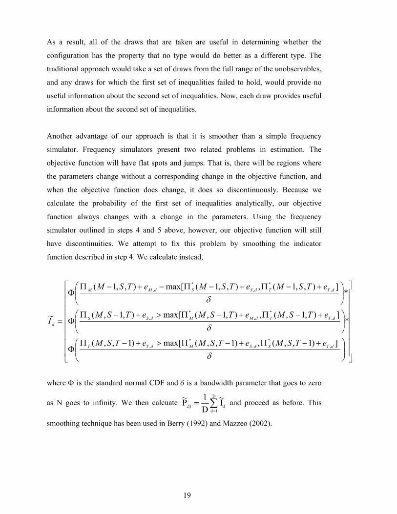
Another advantage of our approach is that it is smoother than a simple frequency

simulator. Frequency simulators present two related problems in estimation. The

objective function will have flat spots and jumps. That is, there will be regions where

the parameters change without a corresponding change in the objective function, and

when the objective function does change, it does so discontinuously. Because we

calculate the probability of the first set of inequalities analytically, our objective

function always changes with a change in the parameters. Using the frequency

simulator outlined in steps 4 and 5 above, however, our objective function will still

have discontinuities. We attempt to fix this problem by smoothing the indicator

function described in step 4. We calculate instead,

+−Π+−Π>+−ΠΦ

+−Π+−Π>+−ΠΦ

+−Π+−Π−+−ΠΦ

=

δ

δ

δ

])1,,(,)1,,(max[)1,,(

*]),1,(,),1,(max[),1,(

*]),,1(,),,1(max[),,1(

~

,*

,*

,

,*

,*

,

,*

,*

,

dTSdSMdTT

dTTdMMdSS

dTTdSSdMM

d

eTSMeTSMeTSM

eTSMeTSMeTSM

eTSMeTSMeTSM

I

where Φ is the standard normal CDF and δ is a bandwidth parameter that goes to zero

as N goes to infinity. We then calcuate I~D1P~

D

1dd1|2 ∑

=

= and proceed as before. This

smoothing technique has been used in Berry (1992) and Mazzeo (2002).

19

REFERENCES

Adams, R., Brevoort K. and Kiser E., “Who Competes with Whom? The Case of

Depository Institutions,” Federal Reserve Board, working paper.

Amel, Dean, and Timothy Hannan, “Defining Banking Markets According to the

Principles Recommended in the Merger Guidelines,” The Antitrust Bulletin 45 (Fall

2000) pp. 615-639.

Amel, D. and Starr-McCluer, M. “Market Definition in Banking: Recent Evidence,”

The Antitrust Bulletin 47 (Spring 2002) pp. 63-88.

Andrews, D. and Berry, S. “On Placing Bounds on Parameters of Entry Games in the

Presence of Multiple Equilibria,” Mimeo (2002), Yale University.

Berry, S. “Estimation of a Model of Entry in the Airline Industry,” Econometrica 60

(July 1992) pp. 889-917.

Biehl, A. “The Extent of the Market for Retail Banking Deposits,” The Antitrust

Bulletin, 47 (Spring 2002) pp. 91-106.

Bresnahan T. and Reiss P. “Entry in Monopoly Markets.” Review of Economic Studies

57 (October 1990) pp. 531-553.

Bresnahan T. and Reiss P. “Entry in Concentrated Markets,” Journal of Political

Economy, 99 (October 1991) pp. 977-1009.

Ciliberto, F. and Tamer, E. “Market Structure and Multiple Equilibria in Airline

Markets,” Mimeo (2003).

Cohen, A. “Market Structure and Market Definition: The Case of Small Banks and

Thrifts,” Mimeo, Federal Reserve Board.

20

“Eliminating the Thrift Charter,” CBO Paper, (June 1997).

Elliehausen, G. and Wolken J. “Banking Markets and the Use of Financial Services by

Households,” Federal Reserve Bulletin 78 (March 1992) pp. 169-181.

Elliehausen, G. and Wolken J. “Banking Markets and the Use of Financial Services by

Small and Medium Sized Businesses,” Federal Reserve Bulletin 76 (October 1990) pp.

801-817.

Feinberg, R. “The Competitive Role of Credit Unions in Small Local Financial

Markets,” The Review of Economics and Statistics 83 (August 2001) pp. 560-563.

Hannan, T. and Prager, R. “The Competitive Implications of Multimarket Bank

Branching,” Journal of Financial Services Research, forthcoming.

Heitfield, E. “What Do Interest Rate Data Say About the Geography of Retail Banking

Markets?” Antitrust Bulletin 44 (Summer 1999) pp. 333-347.

Kwast, M., Starr-McCluer, M. and Wolken, J. “Market Definition and the Analysis

of Antitrust in Banking,” Antitrust Bulletin 42 (Winter 1997) pp. 973-995.

Mazzeo, M. “Product Choice and Oligopoly Market Structure,” RAND Journal of

Economics, 33 (Summer 2002) pp. 1-22.

Pakes, A., “Common Sense and Simplicity in Industrial Organization,” mimeo (2003).

Radecki, L. “The Expanding Geographic Reach of Retail Banking Markets,”

Federal Reserve Bank of New York Economic Policy Review (June 1998) pp. 15-33.

Reiss, P. “Empirical Models of Discrete Strategic Choices,” American Economic

Review, 86 (1996) pp. 421-426.

21

22

Seim, K. “An Emprical Model of Entry with Endogenous Product-Type Choices,”

mimeo, (2003).

Sutton, J. Sunk Costs and Market Structure, MIT Press, Cambridge, (1991).

Tamer, E. “Incomplete Simultaneous Discrete Response Model with Multiple

Equilibria,” Review of Economic Studies, 70, (2003) pp. 147-167.

Toivanen, O. and Waterson, M. “Market Structure and Entry: Where’s the Beef?,”

mimeo (1999).

Tokle R. and Tokle J. “The Influence of Credit Union and Savings and Loan

Competition on Bank Deposit Rates in Idaho and Montana,” Review of Industrial

Organization 17 (December 2000) pp. 427-439.

U.S. v. Connecticut National Bank, 418 U.S. 656, 94 S.Ct. 2788, 41 L.Ed.2d. 1016

(1974).

U.S. v. Philadelphia National Bank, 374 U.S. 321, 83 S.Ct. 1715. 10 L.Ed.2d. 915

(1963).

1 In particular, market structure provides information about economic profits which are

not directly observed.

2 There are several papers studying competition in banking markets that use price data.

Some papers have used survey data, which are often for a particular product in a limited

geographic area. Others have used constructed prices which tend to be aggregated over

different products and geographic areas.

3 United States v. Philadelphia National Bank, (1963).

4 This finding supports the idea of banks providing a cluster of services.

5 United States v. Connecticut National Bank, (1974).

23

6 While it is true that thrifts are able to offer a wider variety of products, it is not clear

that they actually have availed themselves of these options. Pilloff and Prager (1998),

for example, find that thrift C&I lending was limited despite the removal of some of the

restrictions on it.

7 Bank mergers receive closer scrutiny if the post-merger HHI increases by more than

200 to a level above 1800 in any market involved in the merger.

8 Credit Unions are another potentially important competitor that other researchers have

studied in a similar way. For example, Tokle and Tokle (2000) find that local market

shares for credit union deposits are associated with higher interest rates on bank CDs in

Idaho and Montana, and Feinberg (2001) finds that larger credit union deposit shares

are associated with lower bank lending rates on unsecured and new vehicle loans. As

discussed below, it may be possible to extend the type of analysis we do here to include

credit unions, given the availability of appropriate data.

9 Our results do not speak to whether or not the “cluster”, as proscribed in United States

v. Philadelphia National Bank, is the correct standard for bank antitrust analysis.

Rather, the analysis is conducted in a manner that is consistent with the idea of the

cluster.

10 In addition to the papers cited here, see Berry (1992), Toivanen and Waterson (1999)

and Seim (2000). Reiss (1996) provides a discussion of the empirical framework.

11 This specification of the profit function was chosen primarily to make the estimation

tractable. Following Berry (1992) and Bresnahan and Reiss (1991), it can be

interpreted as the log of a demand (market size) term multiplied by a variable profits

term that depends on the number (and product types, in this case) of market

competitors. There are no firm-specific factors in the profit function. The error term

24

( ), ,M

represents unobserved payoffs from operating as a particular type in a given market. It

is assumed to be additively separable, independent of the observables (including the

number of market competitors), and identical for each firm of the same type in a given

market.

12 We assume that firms optimize on a market-by-market basis, which may be

somewhat less realistic for multi-market banks (it is conceivable that such a bank might

enter an individual market to broaden its coverage, even if that market is not

individually profitable). By not analyzing the larger markets that would be more

attractive for this purpose, difficulties caused by this difference should be mitigated.

13 A natural alternative is a simultaneous move game; however, it has been well

established that such a game has multiple equilibria, which precludes straightforward

econometric estimation (Bresnahan & Reiss, Tamer). New methodologies that are

currently being developed to estimate in the presence of multiple equilibria (e.g., Berry

& Andrews, Ciliberto & Tamer) remain beyond the scope of this paper. We proceed

with the Stackelberg assumption, in part relying on the finding in Mazzeo (2002) that

parameter estimates are very similar across various game formulations that generate

unique equilibria.

14 Long-run, dynamic equilibrium models of entry and exit have been proposed, but

have not yet been successfully estimated. See Pakes (2003) for a discussion of recent

progress in this area.

15 Recall that M S Tπ corresponds to the profits of a multi-market bank under the

configuration (M+1,S,T) since a multi-market firm faces M multi-market bank

competitors, S single-market bank competitors, and T thrift competitors.

25

16 Mazzeo (2002) contains proofs of existence and uniqueness. Note that N represents

the product types of competing firms (not including itself). For example, for a

multimarket bank in market (M,S, T), N = (M-1,S, T); for a thrift, N = (M,S, T-1).

17 In addition, these markets have far fewer competitors, making the model more

tractable. More importantly, many of the mergers that raise competitive concerns with

regulators do so because of their effect on smaller markets.

18 This definition is consistent with previous papers that distinguish “single-market”

banks. Note that a bank with 90 percent of its deposits in market A and 10 percent in

market B would, according to this definition, be classified as a single-market bank in

market A and a multimarket bank in market B. This reflects the view that the decision

to operate in market B would be significantly more affected by the role of the branch in

B in the bank’s overall network, as opposed to in market A where the presence of any

branches in market B would be less important.

19 The goal is to make the specification of the competitive effects through as

flexible as possible, while maintaining estimation feasibility. For example, in the cases

where the data indicate the "number" of competitors, we implicitly assume that the

incremental effect of each additional competitor is the same.

g NT( ; )θ

20 For example, for the multi-market monopolist, predicted payoffs = (-1.10 + 0.56 +

1.09 + 0.13 + 0.70 + 1.59) = 2.97.

21 The one exception is the effect of population on single-market bank profits, which is

estimated to be negative. This may suggest that single-market banks have a harder time

servicing large populations or, alternatively, are associated with more personalized

service in smaller markets.

26

22 Such games include a Cournot game with homogenous goods, see Bresnahan and

Reiss (1991), or a Bertrand pricing game with symmetric product differentiation.

23 We should note, however, that all of the cross-type effects involving thrifts are

estimated imprecisely in the border subsample All but one of the cross-type effects are

estimated imprecisely in the total sample as well as the rural subsample.

0 1 2 3 4 5 6+ Total0 13 83 95 95 62 31 34 4131 28 72 80 56 37 27 19 3192 28 39 41 32 25 13 18 1963 8 7 14 20 12 3 7 71

4+ 2 11 7 5 6 6 13 50Total 79 212 237 208 142 80 91 1049

0 1 2 3 4 5 6+ Total0 4 9 22 40 34 30 29 1681 5 28 24 32 24 18 34 1652 10 10 16 25 12 14 19 1063 1 8 9 9 15 8 16 66

4+ 3 5 12 8 16 13 18 75Total 23 60 83 114 101 83 116 580

0 1 2 3 4 5 6+ Total0 0 5 9 10 6 9 15 541 1 2 4 10 10 11 14 522 1 2 6 8 3 5 12 373 0 1 1 5 2 3 9 21

4+ 1 0 1 5 5 2 7 21Total 3 10 21 38 26 30 57 185

0 1 2 3 4 5 6+ Total0 0 0 1 2 8 3 6 201 0 0 1 5 3 1 6 162 0 0 0 1 1 2 6 103 0 0 0 0 1 0 6 7

4+ 0 0 0 4 2 1 10 17Total 0 0 2 12 15 7 34 70

Multi-market

Multi-market

Multi-market

Single-market

Single-market

Single-market

Table 1: Market Configurations

Thrifts=0

Thrifts=3+

Thrifts=2

Thrifts=1

Single-market

Multi-market

27

Variable Mean Std. Dev. Min Max

Population 23,299 19,944 65 99,428Per Capita Income 20,943 3,980 5,475 69,960Farms 617 452 0 4,302Establishements 542 508 1 4,855Occupancy Rate 0.83 0.10 0.23 0.97

N=1,884

Transformation Used: X*=X/(ΣX/N)

Table 2: Market Size Variables

28

Estimate Std ErrorCOMPETITIVE EFFECTS

Effect of first multi-market competitor on multi-market profits -1.0970 0.0646Effect of second multi-market competitor on multi-market profits -0.8193 0.0387Effect of each additional multi-market competitor on multi-market profits -0.7452 0.0195Effect of first single-market on multi-market profits -0.5453 0.1037Effect of each additional single-market on multi-market profits -0.1103 0.0513Effect of first thrift on multi-market profits -0.0329 0.1345Effect of each additional thrift on multi-market profits -0.2745 0.0920

Effect of first single-market competitor on single-market profits -0.9291 0.0357Effect of second single-market competitor on single-market profits -0.7228 0.0346Effect of third single-market competitor on single-market profits -0.5552 0.0375Effect of first multi-market on single-market profits -0.3696 0.1706Effect of each additional multi-market on single-market profits -0.1098 0.0513Effect of first thrift on single-market profits -7.E-06 0.1665Effect of each additional thrift on single-market profits -0.1388 0.1596

Effect of first thrift competitor on thrift profits -1.1889 0.0464Effect of second thrift competitor on thrift profits -0.8918 0.0627Effect of first multi-market on thrift profits -0.0309 0.1768Effect of each additional multi-market on thrift profits -0.0149 0.0691Effect of first single-market on thrift profits -0.1214 0.1633Effect of each additional single-market on thrift profits -0.0004 0.1031

MULTI-MARKET PROFIT SHIFTERSIntercept -1.1031 0.2721Farms 0.5621 0.0568Establishments 1.0887 0.0748Population 0.1258 0.0801Per Capita Income 0.7045 0.1443Occupancy Rate 1.5923 0.2609

SINGLE-MARKET PROFIT SHIFTERSIntercept -2.2107 0.3328Farms 0.7099 0.0570Establishments 0.4843 0.1032Population -0.3261 0.0922Per Capita Income 0.5118 0.2205Occupancy Rate 1.9770 0.3057

THRIFT PROFIT SHIFTERSIntercept -2.0512 0.3262Farms 0.2901 0.0957Establishments 0.3871 0.0950Population 0.1618 0.0936Per Capita Income 0.8546 0.1842Occupancy Rate 0.3763 0.3482

N=1884Log Likelihood = -7192.63

Table 3: Parameter Estimates from Endogenous Market Structure Model

29



Effect of first single-market competitor on single-market profits -0.9429 0.0436Effect of second single-market competitor on single-market profits -0.7294 0.0447Effect of third single-market competitor on single-market profits -0.6030 0.0634Effect of first multi-market on single-market profits -0.3366 0.1948Effect of each additional multi-market on single-market profits -0.1177 0.0424Effect of first thrift on single-market profits -0.0003 0.1582Effect of each additional thrift on single-market profits -0.0748 0.1329

Effect of first thrift competitor on thrift profits -1.2665 0.0744Effect of second thrift competitor on thrift profits -0.7848 0.1050Effect of first multi-market on thrift profits -0.0020 0.2459Effect of each additional multi-market on thrift profits -0.0096 0.0785Effect of first single-market on thrift profits -0.0087 0.1649Effect of each additional single-market on thrift profits -1.E-14 0.1018





Table 3A: Parameter Estimates from Endogenous Market Structure Model Rural Markets

30



Effect of first single-market competitor on single-market profits -0.9258 0.0490Effect of second single-market competitor on single-market profits -0.7252 0.0479Effect of third single-market competitor on single-market profits -0.5286 0.0483Effect of first multi-market on single-market profits -0.4299 0.2922Effect of each additional multi-market on single-market profits -0.1429 0.0890Effect of first thrift on single-market profits -0.0609 0.3897Effect of each additional thrift on single-market profits -0.1600 0.2912

Effect of first thrift competitor on thrift profits -1.1540 0.0653Effect of second thrift competitor on thrift profits -0.9623 0.0850Effect of first multi-market on thrift profits -0.3094 0.2564Effect of each additional multi-market on thrift profits -0.0315 0.1026Effect of first single-market on thrift profits -0.2591 0.3198Effect of each additional single-market on thrift profits -0.0232 0.2094





Table 3B: Parameter Estimates from Endogenous Market Structure Model Border Markets

31

Demographic Variables BakerCounty

SampleMean

Population 22,388 23,299Per Capita Income 19,056 20,943Farms 157 617Establishements 278 542Occupancy Rate 0.93 0.83

Observed Configuration (M,S,T)=(3,0,0)

Expected Profits at Relevant Configurations

Configuration E(ΠM) E(ΠS) E(ΠT)(3,0,0) 0.21 0 0(3,1,0) -0.34 -0.02 0(3,0,1) 0.18 0 -0.49(2,1,0) 0.41 0.09 0(2,0,1) 0.92 0 -0.47

Table 4: Baker County Florida Example

32

MARKET STRUCTURE AND COMPETITION AMONG … · MARKET STRUCTURE AND COMPETITION AMONG RETAIL...

Documents

Transcript of MARKET STRUCTURE AND COMPETITION AMONG … · MARKET STRUCTURE AND COMPETITION AMONG RETAIL...