Market Reaction to Announcements

of Dividend Increases:

Is it Weakening With Time?

A thesis submitted to the College of

Graduate Studies and Research

in Partial Fulfillment of the Requirements

for the Degree of Masters of Science in Finance

in the Department of Finance and Management Science

University of Saskatchewan

Saskatoon, Saskatchewan

By Mark Norton

© Copyright Mark Norton, April 2008. All Rights Reserved.

PERMISSION TO USE

In presenting this thesis in partial fulfillment of the requirements for a

Postgraduate degree from the University of Saskatchewan, I agree that the Libraries of

this University may make it freely available for inspection. I further agree that permission

for copying of this thesis in any manner, in whole or in part, for scholarly purposes may

be granted by the professor or professors who supervised my thesis work or, in their

absence, by the Head of the Department or the Dean of the College in which my thesis

work was done. It is understood that any copying or publication or use of this thesis or

parts thereof for financial gain shall not be allowed without my written permission. It is

also understood that due recognition shall be given to me and to the University of

Saskatchewan in any scholarly use which may be made of any material in my thesis.

Requests for permission to copy or to make other uses of materials in this thesis in

whole or part should be addressed to:

Head of the Department of Finance and Management Science Edwards School of Business University of Saskatchewan 25 Campus Drive Saskatoon, SK S7N 5A7

i

ABSTRACT

This study examines the market’s reaction to announcements of dividend

increases. In particular, it considers the factors that affect the magnitude of abnormal

returns during the days that surround announcements of dividend increases. The objective

is to find whether the market reaction to dividend increases has weakened with the

passage of time and whether market conditions affect the reaction. Eventually, this study

is expected to reveal whether dividends continue to be important to investors.

This research is motivated by the findings of Fama and French (2001). They

suggest that since 1978 firms have had a declining propensity to pay dividends. They

propose that dividends are declining as a result of the ease by which investors can make

homemade dividends through selling small portions of their holdings. They argue that

recent market developments, particularly the introduction of negotiated commissions and

discount brokers, have made homemade dividends easier and less costly. Their results

may suggest that investors are now less interested to receive dividends than in the past.

One objective of this study is to examine whether investor’s preferences regarding

dividend payments have changed over time. This is accomplished by measuring the

abnormal returns following announcements of dividend increases. Benartzi, Michaely,

and Thaler (1997) suggest that the reaction of the market to dividend increases is an

acceptable method of determining the value of dividends to investors.

In addition, this study explores the theoretical factors that may affect dividend

valuation. Previous studies, such as Allen, Bernardo and Welch (2000), suggest that the

existence of debt holders and institutional investors reduce the potential for agency costs

as these stakeholders monitor managers. In contrast, Jensen (1986) suggests that high

ii

cash flows make it easier for managers to spend on perquisites and empire building.

Thus, the potential for agency costs increases. Therefore, paying dividends when cash

flows are high reduces the likelihood of agency costs. At the same time, Benartzi,

Michaely and Thaler (1997) suggest that increasing dividends following higher cash

flows signals management’s expectation that future performance warrants a dividend

increase. Consequently, the agency and signaling theories suggest that investors may

react positively to dividend increases when cash flows are high.

Several observations are obtained from this study. First, investor reaction to

dividend increases seems to have weakened over time. Second, the reaction is different

when the increase is announced in a bear market rather than in a bull market. Third, the

market reaction to dividend increases is less in firms that are more liquid. This finding

may be interpreted as evidence that dividends are valued less in more liquid firms

because it is easier for the investors of these firms to make homemade dividends. Fourth,

the magnitude of the reaction is directly related to the increase in trading volume

following the announcement.

Surprisingly, the evidence disputes the predictions of the agency cost theory of

dividends. This theory states that dividends are valued because they decrease the amount

of cash available to management, which in turn decreases the potential for waste. Given

this theory, it is expected that firms with high debt loads already have agency costs

decreased so the market reaction to their dividend increases would be less than other

firms while firms with high free cash flows would have a greater market reaction to their

dividend increases because of the large potential for waste on management’s part.

Instead, the results suggest that firms with high debt loads experience positive market

iii

reaction following dividend increases while firms with large free cash flows experience

negative reactions. It seems that the signaling theory of dividends is contributing heavily

to this result.

Future research should be directed to investigate the possibility that share

repurchases may be replacing dividends as a way to redistribute surplus cash to

shareholders. In addition, future studies may focus on the signaling theory of dividends as

useful tool to explain the dividend policies of corporations.

iv

ACKNOWLEDGEMENTS

I would like to thank my supervisors Zhao Sun and George Tannous for their

helpful comments and suggestions in order to improve this thesis. I would also like to

thank the members of my defense committee, specifically Abdullah Mamun and Suresh

Kalagnanam. Finally, I would like to thank Craig Wilson who chaired the defense.

I am also grateful for my wife and daughter for their support as I have progressed

through my educational pursuits.

v

TABLE OF CONTENTS

PERMISSION TO USE ..………………………………………………………………i ABSTRACT ………………………………………………………………………...…ii ACKNOLEWDGMENTS ………………………………………………………...…...v TABLE OF CONTENTS ………………………………………………………...…...vi LIST OF TABLES ……………………………………………………………...……viii CHAPTER 1 INTRODUCTION ……………………………………………………. ..1 1.1 Research Questions…………………………………………………..…. 2 1.2 A Brief History of the Evolution of Dividends …….………………….. ..2 1.3 Recent Theoretical Developments ……….………………………………4 1.4 Specific Research that Motivates this Study ……….………………….. . 5 1.5 Summary Findings of this Thesis …………….……………………….. 10 1.6 Concluding Remarks ………..…………………………………………. 10 CHAPTER 2 LITERATURE REVIEW …………………………………………….. 12 2.1 Information Asymmetry and Signaling …………..…………………… 14 2.2 Agency Costs …………….……………………………………………. 19 2.3 Dividend Clientele Models ………….………………………………… 22 2.4 Behavioural Finance Explanations for Dividends ….…………………. 26 2.5 Share Repurchases and Dividend Policy ………………….……….….. 28 2.6 Firm’s Dividend Behaviour Through Time ………………..………….. 33 CHAPTER 3 THEORITICAL ISSUES AND TESTABLE HYPOTHESES ………. 37 3.1 Market Reaction Over Time ………….……………………………… 39 3.2 Market Reaction During Different Market Conditions ………………. 39 3.3 Institutional Ownership ………………………………………………. 40 3.4 The Level of Debt …………………….…………………….…………. 41 3.5 The Level of Free Cash Flows ……………………………..………….. 42 3.6 Market Liquidity of Common Shares ……………….………………… 42 3.7 The Firm’s Q-ratio ………………………………………….…………. 43 3.8 The Change in Volume …………….………………………………….. 43 CHAPTER 4 DATA AND METHODOLOGY …………………………………….. 45 4.1 Sample Requirements ...……………..………………………………… 46 4.2 Data Related to the Independent Variables ………….………………... 46

4.3 Methodology ………………………………………………………….. 54 4.3.1 Determining the Market’s Reaction to a Dividend Increase …….……. 54

4.3.2 Testing to See if the Market’s Reaction to a Dividend Increase is Declining with Time …………………………………………………... 58

vi

4.3.3 Testing to see if there is a Difference in how the Market Reacts to a Dividend Increase in a Bear vs. Bull Market …………………………. 60 4.3.4 Fama-Macbeth Regression ……………………………………………. 62 4.4 Limitations of Data and Methodology ………………………………... 62 CHAPTER 5 EMPIRICAL RESULTS ………………………………………………64 5.1 Preliminary Findings …….…………………………………………….. 67 5.2.1 Investigating the Market’s Reaction to Dividend Increases ………….. 70 5.2.2 Exploring Other Measures of Free Cash Flow ………………………... 74 5.3 Other Model Specifications …………………………………………… 78 5.3.1 Multicollinearity ………………………………………………………. 78

5.3.2 Changing Model Specifications in Order to Increase Explanatory Power ………………………………………………………………….. 81 5.4 The Impact of Market Conditions on the Reaction to Dividend Increases ……………………………………………………………….. 89

CHAPTER 6 SUMMARY FINDINGS AND FUTURE RESEARCH ……………... 96 6.1 Summary of the Findings ……………………………………………….. 97 6.2 Future Research ………………………………………………………….100 REFERENCES ……………………………………………...……………………… 102

vii

LIST OF TABLES Table 1 Expected signs of coefficients for different hypotheses……………….. 60 Table 2 Abnormal and cumulative abnormal returns ………………………….. 68 Table 3 Summary statistics of explanatory variables ………………………….. 69 Table 4 Correlation matrix of explanatory variables …………………………... 70 Table 5 Factors that affect dividend valuation …………………………………. 70 Table 6 Testing alternative proxies for free cash flow measure ……………….. 76 Table 7 Testing for multicollinearity in model ………………………………… 80 Table 8 Using abnormal returns as dependent variable instead of abnormal return standardized by dividend increase ………………... 81 Table 9 Including abnormal volume measure in regression …………………… 83 Table 10 Using lagged values and percentage increase in variables instead of current absolute levels ……………………………………… 85 Table 11 Q-ratio treated as a continuous instead of dichotomous variable ………86 Table 12 Fama-Macbeth regression …………………………………………….. 88 Table 13 Testing for differences between bear and bull markets ……………….. 90 Table 14 Differences in valuation for the time periods 1990-1999 and 2001-2004…………………………………………………………. 92 Table 15 Identifying factors that are significantly different between the two time periods …………………………………………………… 93 Table 16 Summary statistics for explanatory variables for the two time periods…………………………………………………………….. 94 Table 17 Examining the size of firms who declared dividends between the two time periods …………………………………………. 95

viii

CHAPTER 1

INTRODUCTION

This chapter links the objectives of this research to the current state of knowledge

regarding dividends and the theory of the firm. It shows that previous studies do not consider

investors’ interest in receiving dividends or whether investors’ attitude towards dividends is

changing over time or varies with market conditions. Given this gap in the literature, the results

of this study are likely to increase our knowledge of investors’ behaviour towards dividends and

whether investors’ demand for dividend payments is decreasing over time.

The chapter starts with a brief summary of the research objectives. Section 1.2

summarizes the history of dividend payments that started over 400 years ago in Europe as

payoffs from sea voyages. Section 1.3 suggests that the dividend irrelevance propositions of

Modigliani and Miller (1961) do not necessarily apply in practice. Many empirical studies

suggest that the value of a firm is positively related to the size of its dividend payments as

suggested by the dividend discount model. The section goes on to summarize the recent

developments in dividend theory and to describe the recent practices. Section 1.4 briefly reviews

the literature that serves as the main motivation for this research. It suggests that dividend

payments have been changing over time but previous research stops short of considering

investors’ reaction towards dividend payments. Section 1.5 provides a summary of the main

findings of this thesis.

1

1.1 Research Questions

Extensive research, for example Fama and French (2001), DeAngelo, DeAngelo, and

Skinner (2003), and Allen and Michaely (2003), has been done to explain why firms pay

dividends, the appropriate dividend policy, and the alternative ways to distribute earnings to

shareholders. They report that corporations have changed the ways by which they make

distributions to shareholders and the importance they place on dividends.

In contrast, little research has been done to explain the behaviour of investors towards

dividends. This study examines whether over time investors have changed their reaction to

dividend increases. If the market reaction is weakening over time it means that the investors’

demand for dividends is decreasing. Investors, corporate managers, and policy makers would be

interested to know whether investors’ demand for dividends has changed over time. In addition,

this study investigates whether investors’ reaction to dividend varies as a function of different

market conditions. For example, corporate stakeholders and policy makers may be interested to

know whether the reaction of investors to dividend increases during bear market conditions is

different from the reaction during bull markets.

1.2 A Brief History of the Evolution of Dividends

Frankfurter and Wood (1997) provide a brief history of how the payment of dividends

evolved over time. The first dividends were paid during the 16th century when Sea Captains in

Holland and Great Britain began selling financial claims on their voyages. At the end of the

voyage the ship along with all of its cargo were sold and the profits, if any, were then distributed

proportionally to the different owners of the enterprise. These distributions were essentially

liquidating dividends. As time passed these financial claims began trading among different

investors, and sea captains with successful track records began to demand more for a financial

2

claim on their particular voyages. This system further evolved as people realized that the costs

associated with start-up and total liquidation could be avoided if the Sea Captain committed to

several voyages at a time and that a percentage of profits could be paid out each time the Captain

returned to harbour.

In the years that followed these initial sea voyages, more sophisticated corporate charters

were set up in other capital intensive industries such as mining, banking, insurance, utilities, and

railroads. Adam Smith in the “Wealth of Nations” believed that managers of these different

corporations were motivated to pay dividends in order to pacify and thus keep shareholders from

fully monitoring management’s activities. Over the years, economists developed models to relate

the value of a corporation to the value of the dividends it pays. The common conclusion among

financial practitioners and academics was that a firm could increase its value by increasing the

amount of its dividends. This was a direct result of the Dividend Discount Model (DDM) which

continues to be a prominent topic in entry level finance textbooks.1 The DDM says that the

value of any common share is a function of the future dividends expected to be received by the

share and the required rate of return on the stock. This model is defined in the following

formula:

tt

t rDP

)1(10 +=∑

∞

= Eq. 1

where P0 = the price of the stock today

Dt = the dividend to be received at the end of period t

r = the required rate of return

1 For examples, see Ross, Westerfield, Jordan, and Roberts (2007), Fundamentals of Corporate Finance, fifth Canadian Edition.

3

The relation between dividends and the value of the firm as proposed by the DDM

continued to dominate the thinking of financial professionals and academics until the publication

of the dividend irrelevance theorem by Modigliani and Miller (1961). Their seminal work

revolutionized the way theoreticians and practitioners view dividends and ushered the beginning

of new era of research on the role of dividends.

1.3 Recent Theoretical Developments

Under conditions of perfect capital markets, Modigliani and Miller (1961) prove that a

firm’s value is independent of its dividend policy. Their definition of perfect capital markets

means corporations and investors do not pay taxes, transaction costs are negligible, investors are

rational, information is readily available at negligible costs, and investors are as informed as

managers. Unfortunately markets are not perfect and previous studies suggest that the dividend

policy continues to affect the value of common shares as suggested by the DDM. For example,

Benartzi, Michaely, and Thaler (1997), show that a firm’s stock price changes with changes in its

dividend policy. Yet, the factors that affect this relation continue to be topics of debate and

academic research. Propositions attempting to explain the dividend policy include arguments

suggesting that (1) the dividend policy serves as a signal of future earnings growth, (2) investors

feel that cash in hand is superior to an unrealized capital gain, (3) investors value dividends when

the alternative ways to distribute money to shareholders are more costly, and (4) as a way to

decrease the potential waste of resources by management.

In addition, research in the theory of dividends has considered the issues a firm faces

when it decides on a dividend policy. These issues include (1) how much should be given to

shareholders, (2) what should the dividend payout ratio be, (3) how much financial slack does

the firm need to maintain, (4) is the payout level sustainable, (5) and what method of distribution

4

would shareholders prefer. These decisions have far reaching effects on a company’s flexibility

to pursue other activities such as investing in real assets and debt issuance. It is also important to

note that these decisions must be made on a continual basis.

In summary, following the dividend irrelevance propositions of Modigliani and Miller

(1961), many theories and justifications have been proposed to explain why firms continue to

pay dividends and why investors continue to value them. These explanations focus on the

following issues:

Information Asymmetry

An environment of information asymmetry arises when one party has more knowledge

concerning a venture, a transaction, and/or a contract than another party. The literature on

information asymmetry started with Akerlof (1970) who details the information asymmetries

that exist in the used car market. In the context of corporate finance, it is widely accepted that a

firm’s managers have more information regarding the future performance of the firm than its

shareholders do. Many studies, starting with Watts (1973), propose that management may use

dividends to convey information to the market and to shareholders. Thus, dividend payments

decrease the firm’s information asymmetries.

Agency Problems

Jensen (1986) highlights this problem and notes that management has the incentive to

redirect the firm’s money from positive NPV projects to items that directly benefit management.

Some examples of this type of misuse of funds are lavish perquisites, empire building

(purchasing other companies for the sole purpose of managing a larger company), and excessive

management compensation. Jensen (1986) suggests that paying dividends reduces the amount of

excess cash that managers can spend in these ways, thereby reducing potential agency problems.

5

Institutional Constraints

Many institutions, trusts, and endowment funds have imposed constraints on the types of

investments they are allowed to invest in. One such common constraint is to avoid low or non-

dividend paying firms. Previous studies such as Allen, Bernardo, and Welch (2000) propose

arguments, known as the dividend clientele theory, that justify payment of dividends in order to

satisfy the needs of such investors.

Expropriation of Wealth

Some studies, for example Handjinicolaou and Kalay (1984), propose that shareholders

may attempt to expropriate wealth from bondholders and creditors by paying dividends. This

would primarily be a concern if a firm is likely to discontinue its operations in the near future.

Long, Malitz, and Sefcik (1994) explore this proposition and find that managers do not use

dividends to expropriate wealth from others.

Transaction Costs

Early studies such as Bhattacharya (1979) argue that some investors need periodic cash

income from their investments. For such investors, the alternatives include receiving periodic

dividends or selling small portions of their investments. However, selling securities incurs

transaction costs. For some investors it may be more cost efficient to have management issue

dividends to generate income instead of shareholders generating their own income by

periodically selling small parts of their holdings. Fama and French (2001) argue that transaction

costs have decreased over time. Therefore, the desirability for dividends may have decreased as

some investors are now creating their own homemade dividend.

6

Behavioural Issues

Theories of human behaviour may explain the reasons why dividends continue to be

desirable despite the arguments that they may be irrelevant. Behavioural finance studies argue

that investors view capital gains and dividends distinctly and as a result they should not be

considered perfect substitutes for each other. For example, Thaler (1983) describes how

dividends can be viewed as a silver lining during down markets or as an added bonus during bull

markets. Thus, investors may demand dividends even if there are more efficient and cost

effective methods of distribution.

Tax Considerations

Allen and Michaely (2001) suggest that share repurchases are replacing dividend

payments as a way to distribute earnings to shareholders. Theoretically, when a firm has excess

cash and repurchases shares, the shareholders who keep their holding constant should benefit

from the share appreciation that follows the repurchases. The capital gains that may be created

can be realized by selling small portions of their holdings. Essentially, share repurchases create

capital gains to investors while dividend payments create dividend income. Dividends are

considered to be ordinary income by Tax Laws but investors may receive tax credits or may not

pay taxes on dividends. In contrast, share repurchases create capital gains that are usually taxed

at a rate lower than the rate on dividends. Furthermore, even if the tax rates are identical, share

repurchases allow investors to delay the realization of capital gains hence the delay of tax

payments. Overall, tax considerations may make some investors prefer dividend income

(because of tax exemption status) while they make others prefer share repurchases because they

reduce taxes and allow investors to delay the taxation of their returns.

1.4 Specific Research that Motivates this Study

7

Fama and French (2001) document changes in managerial behaviour towards dividends

over the past 25 years. They find firms that pay dividends usually have specific characteristics

that distinguish them from other firms. Once they control for these characteristics, they find that

firms that posses them have a declining propensity to pay dividends. Furthermore, they report

that these characteristics are becoming less common in firms who are now listing on stock

exchanges.

DeAngelo, DeAngelo, and Skinner (2003) consider the same time period that is examined

by Fama and French (2001) and find that the total payout of dividends in real dollars has actually

increased. Combining their results with those of Fama and French (2001) leads to the conclusion

that fewer firms are paying dividends, but those who do pay them are paying larger amounts. In

addition, DeAngelo, DeAngelo, and Skinner (2003) consider the role of special dividends in the

payout policies of corporations. They observe that the use of special dividends as a way to

distribute earnings has been declining. They hypothesize that share repurchases may have

replaced special dividends as a method of returning money to shareholders when the firm does

not want to commit to a higher dividend level. However, they conclude that special dividends are

used less often because they served as a substitute to regular dividends.

Allen and Michaely (2003) provide an extensive review of the payout policies of

corporations including both share repurchases and dividend payments. They suggest that

historically dividends have been the most important form of payout but share repurchases are

becoming a more important part of a firm’s payout policy. For example the average dividend

and share repurchase payouts (payout is defined as dividends paid or expenditure on repurchases

divided by the firm’s earnings) in the 1970s were 38% and 3% respectively. In the 1980s the

8

average dividend payout increased to 58% while the average share repurchase payout increased 9

times to 27%. In addition, Allen and Michaely (2003) report the following observations:

1) Large, established corporations typically pay out a significant amount of their earnings in the

form of dividends and repurchases, and the amount of total payout is increasing.

2) The proportion of dividend paying firms has been steadily declining and that firms who

initiate payout policies are more likely to do so with share repurchases.

3) Individuals in high tax brackets receive a large percentage of cash dividends paid and these

individuals pay substantial amounts of taxes on them. They find that for most of the years

between 1973-1996 individuals received more than 50% of all dividends, but this percentage

declined in the latter parts of their survey. For example, in 1988 individuals received 60% of

all dividends paid. In 1996, this percentage declined to 35%.

4) Corporations smooth dividends relative to earnings, which is not surprising as Lintner (1956)

came to the same conclusion. He found that management sets dividend policy first, and then

adjusts other policies as needed. For example, if a firm was undertaking a large investment

that needed more cash than was available, management wouldn’t consider cutting the

dividend but would instead look for other sources of capital to help fund the project.

5) Data supports the view that share repurchases are more volatile than dividends. Their sample,

which runs from 1972-1998, suggests that on an annual basis aggregate dividends fell only

twice during this period by an average of 3.25%. In contrast, annual aggregate share

repurchases fell six times by an average of 29.46%.

6) The market reacts positively to firms that either increase their dividends or initiate a share

repurchase. In contrast, the market reacts negatively to a firm that decreases its payout

policy.

9

1.5 Summary Findings of this Thesis

The new ideas that are presented in this thesis are the possibility that investors are less

concerned with dividends now than they once were, and that investors’ reaction to dividend

increase is different depending on market sentiment (ie bull vs. bear market). Evidence is found

to support the idea that investor reaction to dividend increases is smaller in the later time periods.

This supports the idea that dividends are no longer as important to investors. There is also

evidence to support the idea that investors value dividends less in a bear market when compared

to a bull market. These are important discoveries as it is the first time that a change in the

reaction to a dividend increase has been noted. Reactions to dividend increases are used because

Michaely Thaler and Womack (1997) find that these reactions can act as a proxy for dividend

valuation, and as a result, the argument can be extended to the possibility that dividends are not

valued as much as they once were, and that they are valued less in a bear market when compared

to a bull market.

Also, in this study many of the relationships of agency theory are explored. Surprisingly,

not a single predicted relationship holds. This means that other dividend theories (ie signalling)

should be explored in future research.

1.6 Concluding Remarks

Dividends continue to be an important tool for the management of modern corporations.

These days, the common practice for many corporations is to pay dividends periodically on a

quarterly basis. The majority of dividend-paying corporations tend to maintain a constant level of

dividends even when earnings are lower than current dividend levels. In such a case,

management takes money from retained earnings or even borrows to keep the stream of

dividends flowing. In studying the history of dividend policies, Frankfurter and Wood (1997)

10

state that dividends have become nothing more than “symbolic” or “token” distributions that are

paid at the discretion of management, and that they do not serve any real economic purpose.

They believe that this is a direct result of the separation between ownership and management and

that paying dividends has become a custom in which management is continually buying

shareholders’ faith that future earnings will be forthcoming. Frankfurter and Wood (1997)

conclude that dividend-payment patterns, more generally known as the dividend policies, are a

“cultural phenomenon, influenced by customs, beliefs, regulations, public opinion, perceptions

and hysteria, general economic conditions, and several other factors, all in perpetual change,

impacting different firms differently.” This study is an attempt to confirm this conclusion using

the market reaction to announcements of dividend increases as an indicator of investors’ interest

in the size and stability of dividend payments.

11

CHAPTER 2

LITERATURE REVIEW

This chapter reviews the prior research on dividends. Specifically it discusses the

theories that try to explain dividend behaviour of firms, and how firm behaviour regarding

dividends and its payout policy has changed.

Section 2.1 reviews the models and evidence for the signalling hypothesis. Signalling

theories try to explain dividends as a signal of private information about the firm that is not

available in standard sources; such as news announcements and audited financial statements.

The main conclusions about signalling theory is that dividends serve as a signal that past

earnings increases are permanent and not transitory.

The second section deals with the models that describe dividends as a way to reduce

agency costs. Agency costs are the result of managers making decisions that are to their benefit,

instead of to the benefit of shareholders. Dividends reduce the potential of managers to waste

money as they reduce the amount of resources at management’s discretion.

Section 2.3 discusses the literature that corresponds to dividend clientele models. These

models feel that dividends are paid in order to make firms attractive to certain clienteles. For

example, some endowment charters state that a firm must pay out a certain percentage of its

profits as dividends in order to be considered for an investment. On the other hand, some

clienteles do not want dividends, as they would rather have the firm reinvest the cash to grow

market share. Thus, there are different investors that seek out different types of investments

based on dividend behaviour.

The fourth section, section 2.4, deals with literature regarding behavioural finance’s

explanation for dividends. Behavioural finance is a relatively new field of study that starts with

12

the assumptions that economic agents are not always rational, and that they do not always want

to maximize their utility. This section deals with different theories that try to explain how

dividends are used and valued by investors in ways that may not be value maximizing.

Section 2.5 discusses the relationship that exists between share repurchases and

dividends. This is important as both are part of a firm’s larger payout policy. This section shows

that share repurchases can serve the same purpose as dividends; mainly, they can reduce agency

costs and send private signals to the market. Share repurchases have the advantage over

dividends in that they are considered to be a one-time payout, whereas the market expects an

increased dividend to be maintained.

The final section, section 2.6, details the literature relating to changes in the pattern of

dividend behaviour of firms. It details the results of papers that show that fewer firms are paying

dividends, and that those that do pay dividends are paying larger ones. It also discusses the

changes that have occurred to share repurchases and special dividends over time.

The primary purpose of this chapter is to fully introduce the literature relating to

dividends. It is necessary to do this in order to introduce the hypotheses that follow in the next

chapter.

13

2.1 Information Asymmetry and Signalling

The assumption that all participants in a market have equal knowledge of that said market

would result in everyone having identical information sets. In this situation all shareholders,

managers, creditors, analysts, and competitors would have equal access to a firm’s financial

results, research and development projects, operations, etc. This obviously is not the case in real

markets. It would be difficult for management to add value to a firm in this situation because

competitors could easily copy a firm’s profitable strategies. Examples of secrets that

management keeps are the Colonel’s famous chicken recipe and Coca-Cola’s exact mixture for

its syrup. Profitability for these companies depends to a certain extent on maintaining

information asymmetries. Without information asymmetries generic colas when compared to

name brand colas would taste the same, cost less, and thereby dominate the market.

If management has to maintain information asymmetries in order to keep its firm

profitable, management must find appropriate signals to let the market know about its quality.

Akerlof (1970) shows that signals must be costly to mimic otherwise poor quality firms will

copy them and a ‘separating equilibrium’ will not be established. A hypothesized separating

equilibrium that has been studied is a firm’s dividend policy. This theory states that high quality

firms should pursue a dividend policy that is too costly for low quality firms to mimic.

The first model to attempt to show how dividends can act as a signalling device was

proposed by Bhattacharya (1979). He proposed that managers signal their firm’s quality to the

market by pre-committing to a dividend policy. The means by which the funds are available to

pay this dividend are known only to management. An assumption of this model is that if the

firm cannot pay for dividends out of internally generated funds, it will turn to more costly

outside financing in order to pay for the dividend. A firm that has higher predictability of cash

14

flows will have lower costs of paying a dividend (because it would less likely need outside

financing) than a firm with unstable and unpredictable cash flows. This results in the low quality

firm finding it too costly to mimic this signal. This model is criticized because firms are not

contractually committed to pay dividends, especially pre-committed dividends. Firms may seek

costly outside financing to pay a dividend, but are under no obligation to do so. This lack of

obligation results in investors not placing any importance on pre-committed dividends.

A second model is proposed by John and Williams (1985). This model assumes that

dividends or net new issues of shares reveal all private information about a firm not conveyed by

corporate audits, financial statements, and other required disclosures. In this model firms paying

higher dividends have more favourable inside information, and thus have higher stock prices.

The optimal dividend policy involves dividend smoothing and higher dividends when the tax

disadvantages of dividends decrease relative to capital gains taxes. This model also explains

why firms would choose the costlier dividend policy over a relatively cheaper share repurchase

program. It is the higher cost of the dividend policy that attracts firms to pay dividends; in

essence, they are purposely incurring the cost because they can afford to do so.

This model also provides an explanation of why firms would pay dividends and

simultaneously seek outside financing to fund new projects. This course of action is justified

because paying a dividend raises the price of the stock, resulting in less dilution of old

shareholders when new equity is raised. This results in the new shareholders paying the correct

stock price.

A third dividend signalling model is proposed by Miller and Rock (1985). This model

assumes that dividends and share repurchases are substitutes for each other and are part of a

larger payout policy. Therefore, a firm can pay a dividend or repurchase shares and send the

15

same signal to the market. In this model, managers are assumed to have private information

about future earnings that will finance future dividend payments and new investments. Larger

dividends (or share repurchases) result in a firm rejecting positive NPV projects and under

investing. Under investing is seen to be a cost that only better firms can incur because inferior

firms cannot afford to pass up on such projects. The equilibrium level of payout policy is

reached when it is high enough that low quality firms cannot reduce their investments enough to

match it.

This model fails however, because it does not consider the differing tax treatments of

dividends and capital gains (capital gains occur when shares are repurchased). Once the

consequence of higher taxes on dividends is considered, the model would have a firm pay out

everything as a share repurchase. As seen in the market, firms still pay dividends so this model

does not adequately explain firm behaviour.

All three models are difficult to test. It is impossible to know if a firm is raising its

dividend to mimic another firm, or if the dividend is raised to signal its own future profitability.

These models also fail to answer what Fisher Black calls “The Dividend Puzzle” (1976). In his

article, Black reviews the question as to why firms pay dividends and points out that for every

argument there is an equally convincing counter-argument. He illustrates this by contrasting two

firms, one that pays a dividend and a second that does not. The market treats the firm that pays a

dividend positively because the dividend represents a return of the shareholders initial

investment. However, the market also acts positively to a firm that does not pay a dividend

because the firm might be signalling that it has many investment opportunities, and that paying a

dividend would result in passing up on some of these. In the second scenario, the investor might

receive the double benefit of capital appreciation greater than the dividend foregone and the

16

lower tax rate applied to capital gains. This illustrates how dividend payment can be interpreted

depending on the investor’s paradigm and the context in which it is paid.

If dividends are indeed sending a signal, what is the signal they are sending? What is the

investing public supposed to infer about a firm’s future if dividends are cut, omitted, raised, or

initiated?

Watts (1973) was the first to try to test the hypothesis that dividend changes forecast

future cash flows and earnings. His primary finding is that there is not a relation between

unexpected dividend changes and future earnings announcements. He also finds that there are

not any abnormal returns in the months surrounding the dividend announcements. Watts’ (1973)

study has limited application because it focuses on monthly returns, which makes it difficult to

differentiate the effects of dividend changes and other information releases.

Healy and Palepu (1988) studied whether there is a significant change in a firm’s

earnings surrounding dividend omissions and initiations. Their study covers the period 1969-

1980 and includes those firms who have not paid a dividend for 10 years (for dividend

initiations) or those firms that have paid a dividend for 10 consecutive years (the dividend

omission study). Their findings indicate that for dividend initiations, firms experience a

permanent increase in earnings for the two years following and one year prior to the dividend

initiation. For dividend omissions, firms are found to have a permanent decrease in earnings for

the year of and the year following the omission. They conclude that dividend

initiations/omissions signal future earnings, albeit that the signal is good for only 1 year with

regards to omissions and 2 years with regards to initiations.

Lintner (1956) stresses that firms only increase dividends when management believes

that earnings have permanently increased. Benartzi, Michaely, and Thaler (1997) test this and

17

try to determine if changes in dividends reflect past or future earnings increases. Their test is

designed to find the relationship (if one exists) between dividend increases and unexpected

future earnings. Unexpected future earnings are defined as the difference between the earnings

that would have been predicted with all the relevant information except for the dividend increase

and the actual earnings of a firm. This implies that firms that increase dividends will have

positive unexpected earnings, and firms that decrease dividends will have negative unexpected

earnings. The authors also hypothesize that the larger the dividend change, the larger the change

in future earnings.

In their study, the only relationship that Benartzi et al. (1997) were able to find was that

dividend changes reflected the permanency of previous earnings increases. They were unable to

find a positive relationship between dividend changes and future earnings changes. This

suggests that if firms are sending a signal about earnings, it’s that the previous earnings increase

is permanent and not transitory. This confirms the earlier work of Watts (1973) and Lintner

(1956) who also found that dividend increases reflect previous earnings increases.

One of the things that has not been studied in regards to dividend and signalling theory is

the possibility that other firm specific characteristics might either magnify or reduce the signal

that dividends send. Some of these characteristics (which will be discussed in future sections in

this chapter) might be a firm’s debt load or the amount of institutional ownership in the firm.

Also, if one subscribes to signalling theory, we do not know if the strength of the signal has

declined over time. This is likely the case as investors have become more sophisticated and are

more likely to know about a firm’s prospects through other means.

18

2.2 Agency Costs

Management constantly makes decisions that affect different stakeholders of the firm.

Management’s decisions are dominated by shareholders’ concerns as other stakeholders have

much less influence. An agency relationship exists when one group is hired to make decisions

on behalf of other groups. Due to divergent interests between groups, these decisions can be

self-serving, or they can cater to the needs of one group at the expense of another.

The agency conflict discussed in this thesis is the relationship between managers and

shareholders. The conflict arises between these two parties because management makes all of

the value enhancing activities but they do not capture all of the benefits that arise from these

activities. This motivates managers to pursue activities in which they do receive the full benefit

of their actions. Easterbrook (1984) discusses this problem and points out two sources of agency

costs: monitoring and risk aversion. Monitoring is essential because it helps to ensure that

management acts in the best interests of shareholders and not other parties. Monitoring

management is prohibitive to small shareholders because a shareholder bears the full cost of

monitoring but only receives the benefits in proportion to his or her holdings.

The other agency cost he discusses is risk aversion on the part of managers. Investors

(assuming they are well diversified) are only interested in non-diversifiable risk; however,

managers have a more vested interest in the success of the firm and are concerned with the firm’s

total risk. This increased interest comes from the possibility of losing their job, having increased

amounts of wealth tied up in the firm, prestige associated with managing the firm, the ability to

consume perquisites, etc. The focus on total risk induces managers to choose lower risk projects

at the expense of shareholders. Shareholders preference is for riskier ventures that will increase

19

their returns and further diversify their portfolios. Management can also change the risk profile

of a firm by altering the firm’s debt to equity ratio.

Easterbrook (1984) proposes that both the monitoring and risk aversion problems can be

avoided if the firm seeks outside financing. Seeking outside financing mitigates the agency

problem because new providers of capital are more effective in scrutinizing management. New

shareholders demand information before investing, and management is forced to cater to these

demands. Firms are forced through this monitoring process more often if they pay regular

dividends because dividends decrease the amount of cash available to management.

Jensen (1986) discusses agency costs in relation to management’s desire to make the firm

larger, even if the firm invests sub-optimally to achieve this goal. Managers prefer to manage

larger firms because doing so is correlated with more power and larger compensation packages.

Management has the opportunity to invest sub-optimally if there are large amounts of free cash

flows in the firm. He defines free cash flows as the amounts of excess cash that a firm has left-

over after it has invested in all positive NPV projects. The greater the amounts of free cash flow,

the greater the potential conflict that exists between management and shareholders. He argues

that shareholders are better served if free cash flows are minimized through dividend payouts.

He also concludes that leverage increasing activities have the same effect on management as the

firm becomes committed to regular interest payments.

In order to decrease the amount of agency costs between managers and shareholders most

executive compensation is now tied to firm performance. Managers are paid substantial bonuses

if the firm meets certain targets, but more importantly managers receive a significant amount of

their remuneration through stock option plans. Stock options allow the manager to benefit more

from their value enhancing activities at the firm.

20

Lambert, Lanen, and Larker (1989) examine the initiation of stock option plans and

changes in corporate dividend policy. A dividend payment reduces a firm’s share price roughly

by the amount of the dividend. Because most stock option plans are not dividend protected, they

hypothesize that the initiation of a stock option plan encourages corporate executives to reduce

dividends. Their results show that the initiation of stock option plans for senior corporate

executives significantly lowers the amount of dividends paid by a firm. These results are

important because they illustrate that management’s use of dividends has evolved, and if it has

evolved, it is a distinct possibility that the market’s reaction to dividend changes has also

evolved.

Lang and Litzenberger (1989) test the two competing free cash flow and signalling

hypotheses. They propose that firms who have excess free cash flows have a tendency to over-

invest, and that over-investment can be measured by Tobin’s q-ratio2. In this study they divided

their sample between firms whose q-ratios are either less than or greater than one. Firms who

have q-ratios less than one are considered to be firms who are over-investing, and firms who

have q-ratios greater than one are considered to be value-maximizing. Lang and Litzenberger

(1989) propose that a firm with a q-ratio less than one (over-investing firm) that increases its

dividend payout would be reducing its free cash flows, and therefore it should be met with a

greater stock price movement when compared to firms whose q-ratios are greater than one.

Consistent with their hypothesis they find that firms with q-ratios less than one have a

significantly larger response to increases in dividend policy than firms with q-ratios greater than

one.

The Lang and Litzenberger (1989) study has a problem in that they simultaneously test

two hypotheses. The first hypothesis is that firms with low/high q-ratios have high/low free cash 2 A firms’ q-ratio is calculated by taking the ratio of market value of equity divided by book value of equity.

21

flows. An example of a firm that wouldn’t fit this description would be Microsoft as it would be

considered to have a high q-ratio and it also has huge amounts of free cash flow. The second

hypothesis is that firms with these different q-ratios have different reactions to a change in

dividend policy. What the Lang and Litzenberger (1989) paper really should report as its

findings is that firms with lower growth prospects as measured by q-ratio have greater reactions

to dividend increases than firms with larger growth prospects. In order to truly test the

hypothesis that free cash flows are an important determinant of how the market reacts to

dividend changes, the free cash flows for the firm should be calculated directly instead of being

represented by the firm’s q-ratio. Once this is done, a test between firms with high and low free

cash flows could be performed to see if there is a difference in market valuation.

Lie (2000) studied the relationship between a firm’s excess funds and firm’s payout

policy and found that dividend increasing firms had excess amounts of cash as compared to peer

firms. This result is consistent with the idea that firms with the greatest potential for

overinvestment decrease that potential by increasing their dividend.

2.3 Dividend Clientele Models

Dividend clientele models are based on the assumption that firms can attract certain

investors by modifying their existing payout policy. A dividend clientele is defined as a set of

investors who are attracted to stocks that have their preferred dividend policy. This is usually

based on their tax and/or liquidity constraints. If a firm tries to attract shareholders that prefer

capital gains the firm would lower dividend payments and increase share repurchases, or if the

firm wanted to attract clientele that preferred dividends it would do the reverse.

Not very much empirical work or research has been devoted to this topical area. This can

be partially attributable to a paper written by Black and Scholes (1974). In this paper they argue

22

that in equilibrium, a firm cannot change its share price by trying to appeal to a different

dividend clientele. They argue this because a change in dividend policy has two offsetting

effects: one clientele group now finds the stock more attractive while another dividend clientele

group finds the stock less attractive. This results in a change in equilibrium, but the firm is still

in equilibrium as it was before the dividend change, therefore the value of the firm remains

unchanged.

That being said, dividend clienteles cannot be ignored. Many institutions face constraints

(either self imposed or regulated) that require them to hold dividend-paying stocks. Mike

O’Neill (CFO of Bank of America) has said, “We’ve got a lot of institutional investors, and a

number of them continue to have dividend requirements that we just try to meet. Many of our

institutional investors will not invest in a company that does not have at least a 2% dividend

yield. . . We think there is a value to having a broad investor base.”3

Allen, Bernardo, and Welch (2000) propose a dividend theory based on tax clienteles.

This model assumes the following: 1) different investors are taxed differently and have different

incentives to do their own due diligence; and 2) dividends are one way of attracting institutions.

The first assumption illustrates the differences between institutions and other investors.

Institutions such as pension funds, university endowment funds, and other non-profit groups are

mostly tax exempt. The relative tax advantage of institutions as compared to other investors

makes dividend paying firms a better purchase for them. Allen et al. (2000) propose that these

institutions have greater incentives to research a firm than small investors do. Institutional

holdings can act as a signal to the average investor of firm quality, and institutions can also

decrease agency costs by selling large blocks of shares to corporate raiders and be actively

involved with corporate governance. 3 Journal of Applied Corporate Finance, Summer 1997, p. 57

23

Their second assumption is reasonable because many institutional charters specify that

securities must pay a dividend in order to be considered for an institution’s portfolio. This

preference stems from the Prudent Man Rule, which states that a fiduciary must “observe how

men of prudence, discretion, and intelligence manage to their own affairs, not in regard to

speculation, but in regard to the permanent disposition of their funds, considering the probable

income as well as the probable safety of the capital to be invested.”4

Allen et al. (2000) specify two models in their paper. The first model is based on

signalling. It concludes that high quality firms attract institutional investors by paying dividends,

and that institutional ownership acts as a signal to uninformed investors. It also concludes that

bad firms dislike attracting institutional investors (because their bad qualities might be revealed)

and therefore do not pay dividends. There are obvious weaknesses with this theory as many top

performing firms have not paid dividends while maintaining high institutional ownership. The

second model is based on agency costs. In this model, dividends attract institutional investors

who ensure that the firm will be run for the benefit of shareholders and not management. Both

models rely on firms purchasing the benefit of institutional ownership through dividends.

There is conflicting research regarding the association between dividend policy and

institutional ownership. Short, Zhang, and Keasey (2002) find a positive link between dividend

policy and institutional ownership. They show that the dividend payout ratio is significantly

higher for firms with more than 5% institutional ownership in the UK. The UK was chosen

because dividends have greater tax advantages for institutions than they do in the US. Thus, the

UK might give more pronounced results and be a better country to test for tax clientele affects.

Dhaliwal, Erickson, and Trezevant (1998) also believe that dividends have a positive effect on

4 The fundamental principle for professional money management, stated by Judge Samuel Putnum in 1830, quoted from Standards of Practice Handbook 1999 by the Association of Investment Management (AIMR)

24

institutional ownership as they examine institutional shareholdings around dividend initiation

dates and found that 80% of firms experience increases in institutional shareholdings over the

three to nine months following a dividend initiation.

Michaely Thaler and Womack (1995) try to identify clientele effects by looking at the

volume that surrounds dividend initiations and omissions. They propose that if dividend

initiations/omissions cause a shift in the clientele, that the common share turnover rate should

increase surrounding these announcements. They find that the increase in volume from day -3 to

+3 (day 0 being the event day) is minor and that there isn’t any significant increase in volume

outside of this event window. One plausible flaw in their methodology is that the shift in

clientele is gradual without any noticeable increase in volume.

Another method to explore the clientele effect that they used was to look at the change in

institutional holdings of stocks prior to and after an omission of a dividend. This is a smaller

sample than the previous method because they were limited to the data available in the Standard

and Poor’s Stock Guide. The average institutional holdings (3 year average) was 30.0% prior to

the omission, and the post 3 year average was 30.9%. This gives further evidence that the

dividend omissions do not produce dramatic changes in ownership.

One thing that has not been studied with regards to institutional ownership and dividend

policy is to see if investors place as much importance on a firm’s dividend policy that have high

institutional ownership as compared to firms that have low institutional ownership. We expect a

difference in investors’ attitude towards these two types of firms if institutional ownership acts as

a signal of firm quality and an effective measure to mitigate agency problems. Specifically, one

would expect that an investor would value a dividend more greatly from a firm that had lower

institutional ownership as compared to a firm with high institutional ownership, ceteris paribus.

25

2.4 Behavioural Finance Explanations for Dividends

Much of economic and financial theory is based on the assumption that individuals act

rationally and consider all available information in the decision making process. However,

researchers have uncovered a surprisingly large amount of evidence that disputes this.

Behavioural finance is a field of study which attempts to better understand this evidence and

explain how emotions and cognitive limitations can explain these results. I will be addressing

specifically how investor’s behaviour towards risk and return may help to explain an investor’s

desire for cash dividends.

The first theory that needs to be addressed is “An Economic Theory of Self-Control” by

Thaler and Shefrin (1981). In this theory they assume that an individual has two internalized

conflicting agents: a farsighted planner and a myopic doer. The planner is concerned with

lifetime utility, and the doer is only concerned with immediate consumption. The planner has to

try and exert some sort of power over the doer so the doer does not consume all of the assets in

the current period. Utility is maximized between the two conflicting agents when the loss of

utility by decreasing current consumption is equal to the gain in utility by having extra future

consumption available.

This theory of self control is built upon by Shefrin and Statman (1984) in which they

describe situations where investors prefer to receive cash dividends rather than capital gains.

Standard finance theory states that investors should be indifferent between capital gains and

dividends in the absence of transaction costs and taxes. Shefrin and Statman (1984) find that

money is not a homogeneous item, and that the source of and future use of money can help

determine how it is used. They determine that individuals use many rules of thumb to assist

26

them in their financing decisions, and these rules of thumb do not necessarily imply maximizing

consumption.

A rule of thumb that Shefrin and Statman (1984) propose that investors use is to spend or

consume dividends and not touch the capital. This rule would stop the myopic doer from over

consuming in the current period by selling too much. This rule also limits the amount of will

power that the planner has to exert on the doer, along with the potential damage for not exerting

enough will power. Another rule of thumb not discussed by Shefrin and Statman (1984) is the

Prudent Man Rule already discussed.

Another relevant theory postulated by Kahneman and Tversky (1982) is the theory of

regret. Kahneman and Tversky (1982) studied individual’s reactions to the following two

hypothetical settings:

1) You take $600 received as dividends (which could have been reinvested with no

transaction costs) and use the money to purchase a television set; or

2) You sell $600 (with no transaction costs) worth of stock and use the proceeds to

purchase a television set.

After the purchase of the TV, the stock rises significantly. If dividends and capital gains

are perfect substitutes for each other, than there shouldn’t be any difference in the levels of regret

between the two cases. However, Kahneman and Tversky (1982) find that the stock sale option

causes more regret. Shefrin and Statman (1984) argue that consumption from dividends may be

preferred to consumption from capital for people who are averse to regret. This means that

capital gains and dividends cannot be treated as perfect substitutes5. Regret aversion can cause

5 In the following section on dividends and share repurchases are treated as perfect substitutes for. As shown by this research, this assumption does not always hold.

27

people to use the same rule of thumb that was discussed earlier under the theory of self control

where investors consume out of dividends and won’t sell any of the capital.

Thaler (1983) discusses how gains and losses are segregated. He believes that people

like to ‘savour’ their gains, which leads to people keeping track of them separately so they can

each be enjoyed individually. He likens it to wrapping Christmas presents separately in order to

experience the pleasure of opening each gift individually. Suppose an investor purchases a stock

and after the purchase the stock price goes down. Thaler (1983) proposes that the dividend is

treated as a silver lining to the price drop and it helps to console the investor. If the stock goes

up, the dividend serves as an added benefit to the price increase. In either case, the investor is

able to get an extra benefit by having the dividend accounted for separately from the capital

gain/loss.

It is important to realize that investors’ perceptions of risk and return can change as time

passes. These changes might occur because of experience, age, knowledge and a host of other

reasons. Because the risk/return profile of the stock market is a function of all those who

participate in it, as time passes, the aggregate view of this profile may change as investors will

have new experiences and more knowledge. As this happens, it is possible that the market will

alter how it reacts to a dividend increase.

2.5 Share Repurchases and Dividend Policy

The previous models and research for the most part discussed and treated dividend policy

and share repurchases as two separate and distinct events; this however is not the case. Share

repurchases and dividend policy are each part of a firm’s larger payout policy, which can include

one method at the exclusion of the other or pursue both methods simultaneously.

28

Lucas and McDonald (1998) solve this dilemma with a model that incorporates both

dividends and share repurchases. This model describes an adverse selection process of share

repurchases. This happens when a firm repurchases its shares at a premium to the current market

price. Most literature treats this as a positive event, but the authors propose that this hurts non-

tendering shareholders as it dilutes their holdings. The resulting equilibrium in their model

results from minimizing the higher tax costs of dividends and the adverse selection costs of share

repurchases. In this model firms in equilibrium with cash to distribute will pay a small dividend

and use the remainder of the cash to repurchase shares. Firms send stronger signals with larger

repurchases. The costly dividend reduces the dilution to current shareholders by decreasing the

share price, and therefore the premium paid on the share repurchase. This decreases the cost of

payout policy to the non-tendering shareholders, whom management should be most concerned

with as they are the shareholders following the repurchase.

Brennan and Thakor (1990) also propose a model that considers both share repurchases

and dividends. This model is based on information asymmetries that exist amongst the investors

in the firm; specifically, some investors through their own due diligence have acquired more

information about the firm than others. This information allows those investors to make better

decisions when the firm decides to pursue a share repurchase. The informed investors will

tender the stock when the repurchase price exceeds the stock’s true value, and will keep their

holdings when the tender price is less than this value. In either case, the uninformed investor is

worse off when the firm uses a share repurchase to distribute excess cash. A dividend policy

allows all investors to receive an equal or pro rata amount of the firm’s profit and the informed

investors are not able to take advantage of their superior information. As a result, the

29

uninformed investors prefer dividends to repurchases assuming that the tax burden of dividends

is not too large, and the informed investor always prefers share repurchases.

In the previous section on signalling, a firm’s dividend policy acted as a signal to

uninformed investors. Because share repurchases and dividends are each part of a firms total

payout policy, it is possible that share repurchases can signal the same information that dividends

do about a firm’s prospects. Comment and Jarrell (1991) propose that share repurchase

programs that serve as the best signal are those that increase the amount of risk the firm’s

managers assume through the repurchase. Assuming that managers do not tender their shares

during a repurchase period, they suggest that the manager’s risk increases when: 1) the initial

holdings of management are large; 2) the greater the offer premium over the current price; and 3)

the larger fraction of equity sought in the offering.

There are three types of share repurchases that are used in the market: 1) Dutch-Auction;

2) Fixed-Price; and 3) Open-Market. In a Dutch auction repurchase a firm solicits offers from its

shareholders, and then offers the lowest price needed in order to get the required number of

shares sought in the offer. A fixed price offer has a fixed number of shares being sought at a

fixed price. The offer price is higher than the current market price and is usually at a 20-25%

premium. An open market program has the company buying the shares on the exchange for a

variety of prices over an extended period of time. Because the methods of these repurchases are

different, it is expected that they will give different signals to the market.

Comment and Jarrell (1991) study the effectiveness of the signals that the different

repurchase methods may give. They propose that the fixed price tender offers will dominate

both open market repurchases and Dutch auction offers. They hypothesize this because fixed

price tender offers release more information (specific price and amount of shares) by corporate

30

insiders. Both Dutch auction tender and open market repurchases rely on the price discovery

process of the market, and management never specifies what it thinks the stock is worth. False

signalling can occur with fixed price offers when the premium offered over the current stock

price is not maintained after the repurchase is completed. This cost represents a dividend paid to

tendering shareholders (as they received more for the stock than what it was worth) that is paid

by the non-tendering shareholders.

They find that each repurchase program is associated with above average returns on the

announcement day. Abnormal returns are 11%, 8%, and 2% for the fixed price, Dutch auction,

and open market repurchases respectively. This shows that the market values fixed price tender

offers more than the other methods, and they propose this because it gives more information to

the market than the other methods do. There is also evidence that the repurchase premium is

larger (meaning a greater signal) when the recent performance of the stock has been poor.

Comment and Jarrell (1991) note that most of the buy back activity is through Dutch auctions

and open market transactions, and conclude that other market factors are important and help

determine which repurchase method firms choose.

The primary benefit of a share repurchase over a dividend is that investors can defer taxes

on their investments until they want to assume the tax burden. DeAngelo (1991) discusses this

dilemma and assumes that tax deferral and consumption deferral are supplied goods. The

implication for this model is that if firms adopt low payout policies to take advantage of tax

deferral, the market will be over supplied with future consumption. This excess supply of future

consumption causes the current market prices to react and brings the stock market back to

equilibrium. This equilibrium is reached even if investors are allowed to borrow or lend to

rearrange their personal consumption because such transactions wouldn’t affect the aggregate

31

level of consumption. This model helps explain why firms do not exclusively use share

repurchases in spite of its tax advantages.

Just as firms can use share repurchases instead of dividends as a signal, firms can also use

share repurchases to mitigate agency costs. In order to study the differences between share

repurchases and dividends, a number of studies have been performed that analyze the cash flows

of firms surrounding these events. Lie (2000) finds that all firms who increase their payout

policy in a given year have increased cash flows prior to the announcement. Firms that pay a

special dividend or pursue a share repurchase program have incurred large, non recurring cash

flows prior to the announcement and have cash flows that revert to the mean once the payout has

been completed. Firms that increase their regular dividend have increases in operating cash

flows that continue after the dividend has been increased. Jagannathan, Stephens, and Weisbach

(2000) have similar findings but have two additional conclusions. They find that repurchasing

firms have more volatile cash flows before and after the distribution, and also find that firms

repurchase stock following poor stock market performance and increase dividends following

good stock market performance.

Both Lie (2000) and Jagannathan et al. (2000) show that firms are able to maintain

financial flexibility by distributing excess funds with a share repurchase or special dividend

instead of increasing their regular dividend. This confirms the work of Lintner (1956) who

proposed that firms only increase dividends once cash flows have permanently increased.

Jagannathan et al. (2000) found that firms increase their dividends more during economic peaks

and decrease them during economic downturns. They also found that repurchases account for

most of the year-to-year variation in a firm’s total payout.

32

Guay and Harford (2000) perform a similar analysis to both Lie (2000) and Jagannathan

et al. (2000) but they also examined the stock price reaction to both share repurchases and

dividend increases. Guay and Harford (2000) hypothesize that dividend increases will send a

better signal to the market than share repurchases as dividends represent an increase to

permanent earnings. Their hypothesis predicts that dividends and share repurchases give

different signals regarding future cash flows. They find evidence to support this as the stock

price reactions to announcements of dividend increases are significantly greater than the

reactions to share repurchases. Also, in addition to previous studies that focused on comparing

cash flows prior to and after a firm’s distribution, they compare the cash flows of firms who

change distributions to a control group that does not change its annual payout. They find that

operating cash flows are similar between the control group and firms who engage in one time

payouts (share repurchases and special dividends), and are different between the control group

and firms that increase regular dividends.

As investors have begun to realize the advantages of using different forms of payout, it is

likely that they have changed the way they value dividends both as a signal and as a way to

decrease agency costs. That being said, dividends and share repurchases cannot be treated as

perfect substitutes for each other as was outlined in section 2.4.

2.6 Firm’s Dividend Behaviour Through Time

Fama and French (2001) studied dividend behaviour of firms from 1926-1999 and find

that the tendency for a firm to pay dividends is on the decline. In 1978, the proportion of non-

financial and non-utility firms that paid a dividend was 66.5%, and this has steadily declined to

20.8% in 1999.

33

Fama and French (2001) study this pattern and try to identify the cause of such a dramatic

shift in the amount of firms paying dividends. They find through logit regressions that dividend-

paying firms tend to share the following three common characteristics relative to non-dividend-

paying firms: higher profitability, fewer investment opportunities, and larger size. They show

that newly listed firms from 1978 onward tend to be smaller, unprofitable ones with many

investment opportunities.

This does not explain all of the reduction though. They find that there is a lower

propensity to pay dividends among all firms regardless of size, investment opportunities and

profitability. There has been an increased number of share repurchases over this time period but

it is argued that since share repurchases are primarily the territory of dividend payers, that this

cannot explain the decline in the percentage of firms that pay dividends. They contend that the

primary effect of increases in share repurchases is to increase the already high cash payouts of

dividend payers.

They believe that some, but not all of the possible reasons for such a decline are: 1) lower

transaction costs for selling stocks enabling investors to create home made dividends; 2) larger

stock option holdings for managers who prefer capital gains to dividends; and 3) better corporate

governance that lowers the importance of dividends in controlling potential agency conflicts.

A study over the same time period was performed by DeAngelo, DeAngelo, and Skinner

(2003) who find that aggregate real dividends increased over the time period of the Fama and

French (2001) study. At first this seems to contradict Fama and French (2001), but DeAngelo et

al (2003) find that the reduction in dividend payers occurs primarily among firms who paid very

small dividends, and that the increase in real dividends from the firms that pay large dividends

dominates the effect of losing many firms that pay these small dividends. Combining the

34

findings of these two studies results in the conclusion that there has been an increase in the

concentration of dividend payers.

Many people have assumed that share repurchases have displaced special dividends in a

firm’s corporate payout policy. DeAngelo, DeAngelo, and Skinner (2000) study special

dividends over time and conclude that special dividends have disappeared because they were

close substitutes for regular dividends, not because they were displaced by the increased use of

share repurchases. They reach this conclusion for a number of reasons. First, they show that

most firms who paid special dividends paid them on a regular basis. Firms who paid special

dividends did so on an average of once every other year. Second, they also show that when firms

reduced special dividends they simultaneously increased regular dividends. Third, their data

shows that the disappearance of special dividends coincides with all firms adopting uniform

dividend policies that pay quarterly. Finally, firms were more likely to increase their regular

dividends once they stopped paying special dividends.

They believe that share repurchases did not displace special dividends because they

cannot find any correlation between the decline in special dividends and the increased use of

share repurchases. The decline in special dividends started prior to the rise of share repurchases,

and if share repurchases replaced special dividends, DeAngelo et al. (2000) argue that

replacement cannot explain the gap between the two events. Also, firms who once paid special

dividends are no more inclined to start a share repurchase program than firms who never paid

such a dividend.

One potential explanation of the change in firms’ dividend behaviour is that fewer firms

are paying dividends because investors do not want them to. This idea has not yet been

addressed in the literature and is one of the hypotheses to be tested. Also, no one has studied

35

whether the market reacts to dividend increases differently between bull and bear markets. An

analysis of this type using current data was not possible until recently because of the long bull

market that started in 1983 and ended in approximately 2000. It is quite possible that dividends

are treated differently during bear and bull markets as these varying market conditions present

different paradigms in which to make judgments through.

36

CHAPTER 3

THEORETICAL ISSUES AND TESTABLE HYPOTHESES

This chapter introduces the hypotheses and discusses the motivation and the theoretical

arguments that support each. In total there are eight hypotheses.

Hypothesis 1 deals with the possibility that the market reaction to dividend increases has

changed over time in a consistent and noticeable pattern. It postulates that the reaction has

weakened, and if true, it suggests that investors’ demand for dividends has decreased over time.

This is motivated by the observation of Fama and French (2001) that firms exhibit declining

propensity to pay dividends.

Hypothesis 2 deals with the possibility that the market reaction to dividend increases

varies depending on the conditions of the market. In particular, the possibility that investors treat

dividends differently in bear markets than they do in bull markets is tested.

Hypotheses 3-8 examine respectively the relation between the market reaction to

dividend increases and institutional ownership, debt load, free cash flow, liquidity, Tobin’s q-

ratio, and trading volume. Previous studies suggest these variables may explain the differences in

the market reactions to dividend increases. Hypothesis 3 is motivated by the argument that high

institutional ownership reduces agency costs and works as a signal of firm quality to the market.

In the presence of institutional ownership, the role of dividends to act as a signalling device and

reduce agency costs is likely dampened. So it is postulated that the size of institutional

ownership helps explain cross-sectional differences in the impact of dividend increases.

Hypothesis 4 states that the level of debt in the capital structure can explain differences in

the market reaction to dividend increases. In theory, debt holders monitor managers to ensure

compliance with debt covenants. This monitoring may reduce agency costs.

37

Hypothesis 5 is motivated by the argument that free cash flows are positively related to

agency costs. Dividend increases by firms that have large free cash flows would be a strong

signal to the market that managers are not interested in consuming perquisites or empire

building. Therefore, Hypothesis 5 postulates that the market reaction to dividend increases is

more pronounced for firms with larger free cash flows.

Hypothesis 6 is motivated by the argument that the decline in the propensity of firms to

pay dividends is due to decline in transaction costs and to the ease with which investors can

create home-made dividends. It is believed that the more liquid a firm is, the easier it is to

create a home-made dividend in it. This should result in a smaller market reaction to dividend

increases for more liquid firms.

Hypothesis 7 deals with the role of the Tobin’s q-ratio in explaining the market reaction

to dividend increases. Traditionally, a high q-ratio is associated with firms that have high growth

opportunities. Yet, previous studies have used the q-ratio to proxy for agency costs instead. In

this study, agency costs are accounted for directly by computing the free cash flow for each firm.

The q-ratio is then tested to see if it is still an important factor in determining the market’s

reaction to a dividend increase.

Hypothesis 8 tests whether the market reaction to dividend increases is related to the

increase in trading volume following the announcements of the dividend increase. While the

relation between volume and share price has been tested in dividend omission and deletion

studies, it has never been tested for using a sample that focuses on dividend increases.

As a note, hypotheses 7 and 8 were developed as the research progressed on this thesis.

38

3.1 Market Reaction Over Time

Previous studies clearly suggest that the behaviour of firms in regard to dividends has

changed over time. Fama and French (2001) show that firms in general have a decreasing

propensity to pay dividends. DeAngelo, DeAngelo, and Skinner (2000, 2003) report that on

average that firms who paid dividends in the past are now paying larger ones. In addition, they

find that special dividends have disappeared.

There is little research regarding the possibility that investors may have changed their

behaviour towards dividends. Some of the possible reasons for this change would be better

corporate governance, more timely releases of new information, and better informed investors.

These market improvements may have reduced the significance of dividends as a way to reduce

agency costs or signal firm quality. If these functions are no longer needed, it is possible that the

importance of dividends has declined.

Given this literature and reasoning, the following hypothesis is tested:

Hypothesis 1: The market reaction to dividend increases is declining over time

3.2 Market Reaction During Different Market Conditions

It is rational to expect that investors are concerned about total returns, the sum of capital

gains return and dividend yield. Previous studies suggest there are several reasons why investors

may react differently to dividend increases based on market conditions. Thaler (1983) suggests

that investors may treat dividends as a silver lining when capital gains return is negative. On the

other hand, when capital returns are positive he states that dividends may be treated by investors

as an added bonus. Previous studies in behavioural finance, such as Shefrin and Statman (1984),

propose that investors do not act consistently in all circumstances. They find that money is not a

39

homogenous item, and that its source can determine how the money is spent. They find that

investors treat money differently if it is received as a capital gain or dividend.

If this is true, then it is possible that market conditions can help determine the value that

investors place on different components of return.

It may also be the case that market participants place greater importance on the

possibilities that dividends signal private information and reduce agency costs in bear markets.

Signalling could take on a greater role in such a market as many firms see decreasing share

prices without a corresponding decrease in future outlook. Also, agency costs could be seen to

be greater in a bear market as there is a likely decreased amount of positive NPV projects to

invest in.

This leads to the second hypothesis to be tested:

Hypothesis 2: The market reaction to dividend increases will be greater during bear markets than

in bull markets.

3.3 Institutional Ownership

Allen, Bernard, and Welch (2000) propose a model in which dividends serve to attract

institutional investors. These investors have a greater incentive and ability to research a firm’s

future cash flows than the marginal investor. They also have better abilities to monitor

management which reduces the potential for waste. Allen et al. (2000) also contend that

institutions serve as a signal to the average investor. As dividend theories propose that dividends

serve to act as a signal and reduce agency costs, dividends are likely to be redundant in firms that

have high institutional ownership.

If this is true, it would be expected that such firms would have smaller reactions to a

dividend increase. This has not yet been tested. Previous tests on institutional ownership have

40

primarily focused on dividend initiations and omissions. For example Dhaliwal, Erickson and

Trezevant (1998) find that institutional holdings increase after a firm initiates a dividend.

The relationship between a firm’s institutional holdings and its increase in dividend leads

to the third hypothesis:

Hypothesis 3: Firms with high institutional ownership will have smaller market reactions to

dividend increases.

3.4 The Level of Debt

Jensen (1986) argues that debt holders reduce agency costs as they monitor managers to

insure the firm is complying with debt covenants. Covenants are usually designed to restrict

management’s ability to take actions that may transfer value from bondholders to common

shareholders. A restriction on dividend levels increases is often one of these covenants.

Therefore, a dividend increase by a firm that has a high debt ratio indicates the firm has received

approval from debt holders that it is capable of paying a higher dividend. This approval may act

as a signal to the market, and if this is the case, the market should react in a positive way.

In contrast, interest payments may be viewed as a substitute for dividend payments in that

they reduce the discretionary cash flows available to managers. According to this view, a firm

that is highly indebted presents managers with fewer opportunities to consume perks and pursue

empire building. If this argument is true, then shareholders will value a dividend increase less in

firms with high debt levels because discretionary cash flows are already reduced. In this case, a

dividend increase may be seen as of no value to shareholders. As a result, the reaction to a

dividend increase may be insignificant or negative. This is called the agency effect.

These arguments lead to the fourth hypothesis:

41

Hypothesis 4: The market reaction to dividend increases is stronger for firms that have high debt

ratios if the signal effect outweighs the agency effect. If the agency effect

outweighs the signal effect, then it is expected that the market reaction will be

negative to firms who increase their dividend.

3.5 The Level of Free Cash Flows

One of the major themes in the dividend literature is that dividends reduce the potential

for agency costs by reducing the amount of cash available to management. Lang and

Litzenberger (1989) find that firms with q-ratios less than one have a larger reaction to dividend

increases than firms with q-ratios greater than one. They suggest that the market reactions are

directly related to the amount of cash flows available to managers. Higher reactions should be

associated with firms that have high cash flows. In their view, the levels of cash flows available

to managers are inversely related to a firm’s q-ratio.

In this study, free cash flows are calculated for each firm in the sample. The variable that

represents cash flows is included in the regressions to test the hypothesis:

Hypothesis 5: Dividend increases that are announced by firms that have large amounts of free

cash flows will generate stronger market reactions than dividend increases that are

announced by firms that have small amounts of free cash flow.

3.6 Market Liquidity of Common Shares

This research question stems from Fama and French (2001). They argue that transaction

costs have decreased over time and information is cheaper to acquire and readily available. They

observe that the propensity to pay dividends dropped significantly in 1978 and they partially

attribute this drop to the introduction of negotiated commissions three years earlier. They

conclude that it is now easier for investors to periodically sell a small amount of their holdings to

42

create home-made dividends. Thus, investors may not need the quarterly dividend distributions

to receive regular cash flows. It is proposed that it is easier to create these home-made dividends

the more liquid a firm is. There is no prior research that investigates the relation between the

liquidity of a firm’s common shares and its dividend policy.

These arguments lead to the following hypothesis:

Hypothesis 6: Firms with greater liquidity will have smaller market reactions to a dividend

increase than firms with low liquidity

3.7 The Firm’s Q-ratio

Lang and Litzenberger (1989) find that firms with q-ratios less than one have greater

reactions to dividend increases than firms whose q-ratios are greater than one. They argue that

the q-ratio is inversely related to the level of free cash flows available to firms. Based on these

arguments, they justify their conclusions on the basis that dividend increases associated with low

(high) Tobin’s q-ratios are observed because these firms have high (low) free cash flows.

In this thesis, free cash flows are calculated directly from the publicly available financial

statements of the sample firms. The data shows no relationship between the firm’s free cash flow

and its q-ratio. This raises the question of whether the q-ratio is still an important factor in

determining the market’s reaction to a dividend increase. Traditionally, the Tobin’s q-ratio is

used as a proxy for the growth opportunities of the firm. These arguments lead to the following

hypothesis:

Hypothesis 7: Dividend increases by firms that have low growth opportunities produce stronger

market reaction than dividend increases by firms that have high growth

opportunities.

3.8 The Change in Volume

43

Previous studies have been done on volume changes and dividends. The primary purpose

of these studies is to identify clientele effects. In particular, Michaely, Thaler, and Womack

(1995) try to determine if there are volume changes surrounding dividend initiations and

omissions, which would indicate clienteles shifting into and out of those stocks. They find that

there are only minor changes in volume surrounding the omission or deletion dates. Without

significant results, they propose that the clientele effect may take place gradually and thus it

would be undetectable using current techniques.

In this study, it is proposed that volume changes surrounding the dividend increases can

explain some of the variations in the market’s reaction to these increases. This leads to the

hypothesis:

Hypothesis 8: The market’s reaction to a dividend increase is positively associated with the

change in volume following the announcement

44

CHAPTER 4

DATA AND METHODOLOGY

This chapter reviews the sample requirements and the methodology used to test the

hypothesis. Section 4.1 describes the sample and the conditions under which a firm may be

included in it. Section 4.2 explains the procedures that are followed to collect the data related to

each firm in the sample. In particular, it explains how the firm’s free cash flows, debt to equity

ratio, the percentage of outstanding shares held by institutions, common share turnover, q-ratio,

and volume changes are measured.

Section 4.3 describes what is meant by the market reaction to dividend increases and

explains the procedure by which this reaction is measured. Essentially, the market reaction is

defined as the percentage abnormal return divided by the percentage increase in dividends.

Section 4.4 specifies how the hypotheses are tested. Section 4.4.1 presents the Ordinary

Least Squares (OLS) regression model that is used to test most of the hypotheses stated in

Chapter 3. Section 4.4.2 describes the process by which the second hypothesis is tested. This

hypothesis is concerned with the possibility that the market’s reaction to an increase in dividends

during a bull market is different from the reaction during a bear market. Section 4.4.3 gives the

details of the Fama-Macbeth (1973) regression which is also used in the analysis. Section 4.5

briefly discusses the limitations borne from the methodology used and some underlying

assumptions.

45

4.1 Sample Requirements

This thesis studies the behaviour of stocks in the United States surrounding

announcements of dividend increases. The study covers the twenty-year period from 1985 to

2004 inclusive. This time period was chosen for two reasons. First, it coincides with the sample

period of Fama and French (2001) who identified the firm’s declining propensity to pay

dividends. Second, some data required for this thesis are retrieved from the Compustat North

American Database. This database provides information for the most recent 20 years.

In order to be included in the sample, a firm must:

1) Be listed on one of the NYSE, NASDAQ or AMEX exchanges,

2) Have daily return data available from CRSP;

3) Have increased its quarterly dividend by at least 10%;

4) Have paid no special dividends and made no quarterly dividend increases during the

previous 6 months;

5) Not be a utility firm as determined by the firm’s SIC code;

6) Be paying dividends in U.S. dollars without any withholding taxes on the dividend;

7) Have had no stock splits during the month that precedes the dividend increase

announcement; and

8) Have the dividend declaration date and the increase of the dividend recorded in the

annual publication of Moody’s Annual Dividend Record from 1985-1998 and in

Mergent’s Annual Dividend Record6 from 1999-2004.

The sample requirements listed above resulted in a total of 919 total firms being included with

2,303 different observations.

4.2 Data Related to the Independent Variables 6 Moody’s changed the name of its publications from Moody’s to Mergent’s in 1999

46

Information related to a number of variables is needed in order to carry out the analysis.

The firm’s free cash flow, debt to equity ratio, and liquidity are obtained from the Compustat

North American Database. Information related to institutional holdings is obtained from the

Thomson Financial Database.

Free Cash Flow

Free cash flows are important to a firm because they represent the resources that are

available for discretionary use by management. Some of these uses could enhance shareholder

value such as positive NPV projects, dividend payments, debt reduction, and share repurchases.

However, it is also possible for management to spend discretionary money on negative NPV

projects such as perquisites and pet projects. For this reason it is hypothesized that investors

value dividends because it decreases the amount of money that managers may potentially waste.

Lang and Litzenberger (1989) conclude that firms with larger free cash flows experience a larger

abnormal return than firms with smaller free cash flows. In their methodology they divide their

sample into firms with q-ratios above and below one, and assume that firms with q-ratios less

than one have larger free cash flows. For this thesis, free cash flows are computed directly and

then tested to see if the level of free cash flow has a significant relationship with the market’s

reaction to a dividend increase.

One of the problems associated with calculating free cash flow is that there is no single

definition that is accepted by all financial professionals. Most definitions7 result in a similar

figure but there are slight differences in how this figure is calculated. For example, one

definition might start with net income and another might start with operating income prior to

depreciation expenses. The first definition will add back depreciation and the second will add

7 For examples see “The Analysis and Use of Financial Statements” by White, Sondhi and Fried (1997) or “Investment Valuation” by Damodaran (1996).

47

income from non-recurring items. Eventually the two approaches produce similar results. The

definition of free cash flow which is used in this thesis is:

FCF = NI + DEP – DIV – CAPX ± Δ NWC ± DEF TAX ± NET DEBT Eq. 2

where FCF - Free Cash Flow

NI - Net Income

DEP - Depreciation

DIV - Cash Dividends Paid to Shareholders

CAPX - Capital Expenditures

Δ NWC - Changes in Net Working Capital

DEF TAX - Deferred Taxes

NET DEBT - Net New Debt

Lie (2000) also tried to find a relationship between a firm’s cash flow and abnormal

returns when a firm increases its dividend but was not able to do so. He used a different measure

of cash flow and abnormal returns. His definition of cash flow was called ‘undistributed cash

flow’ which is defined as operating income before depreciation minus interest expenses, taxes

and dividends. The definition presented here is more thorough as it includes all of Lie’s (2000)

variables plus the cash flows that result from debt, deferred taxes, capital expenditures and

changes in networking capital. Lie’s (2000) definition of the dependent variable abnormal return

is also different. He used raw abnormal returns (as described in the next section) while the

dependent variable used in this thesis is abnormal returns standardized by their dividend

increase. Thus, the abnormal return for a 10% dividend increase in Lie (2000) was treated the

same as an abnormal return associated with 50% dividend increase. The standardization is

necessary because a larger increase in dividends should relate to a larger abnormal return.

48

Hopefully by making these changes I will be able to identify a relationship between dividend

valuation and cash flows.

The net income figure is the starting point for this measure and it represents the income

or loss of a firm for a period. It is determined as the sum of income from all sources minus all

expenses and losses. Note that this net income measure includes the cash flows from

extraordinary items and discontinued operations. Alternatively, these cash flows may be

excluded to obtain the free cash flow from operations. For this thesis all cash flows that are

available to a manager are considered important as the cash can be used improperly regardless of

how it was obtained. The net income data used in this study are obtained directly from

Compustat (mnemonic code is NI).

Depreciation is a non-cash expense that reduces the cash flows a firm may report as net

income. It is technically cash set aside for the purpose of replenishing depreciable assets.

Therefore, depreciation is added back to net income to obtain the actual amount of cash available

to managers. The depreciation amount is obtained from the Compustat database (mnemonic

code is DP).

The amount of cash dividends paid to shareholders is subtracted from net income to

obtain free cash flow. It may be argued that cash paid as dividends should not be deducted as in

theory dividend payments are discretionary and may be discontinued by management. However,

in practice dividend payments are not entirely discretionary and freely determined by

management. It is well documented (for example see Lintner 1956) that dividends are smoothed

over time and rarely cut. In extreme cases when cash resources are not enough, management will

find other sources of capital to pay dividends rather than reduce or suspend them. The amount of

dividends paid is obtained from Compustat (mnemonic code is DV).

49

Capital expenditures are subtracted from net income to find free cash flow. This is done

as capital requirements need to be made to maintain the firm’s current productive capacity.

There are two possible ways to estimate capital expenditures; these are historical cost

depreciation and total capital expenditures made during a period. If capital expenditures for a

period equalled depreciation then this would nullify the depreciation expense that was previously

added back. As the depreciation expense is arbitrary, it would be nothing more than coincidence

if it equalled the capital expenditures needed to maintain current capacity. The second

alternative relies on the capital expenditures a firm identifies on the cash flow statements

(Compustat mnemonic code is CAPX). This figure is generally regarded as the better choice and

is therefore the method used here even though the discretionary capital expenditures are not

distinguishable from necessary expenditures. Ideally, necessary capital expenditures are not

included in this calculation because managers do not have a choice regarding these expenditures,

and the free cash flow measure tries to identify cash flows that management can make choices

with.

Changes in net working capital are needed to calculate free cash flow. Net working

capital for any given year is defined as current assets minus current liabilities. Both of these are

found directly from Compustat (mnemonic codes are ACT and LCT respectively). What is

important for the measurement of free cash flow is the change in net working capital from the

previous year. For example, an increase in current liabilities in one year while holding all else

constant (except for a general asset account which matches the increase found in current

liabilities) means that a firm has increased its assets through increasing liabilities. This is

considered to be a source of or increase to cash. The change of net working capital for the years

1986-2004 is calculated by subtracting the previous year’s working capital from the current year.

50

If this calculation yields a positive number (current assets increased or current liabilities

decreased or both) this means that the firm has decreased its cash flows, and the opposite is true

if this number is negative. This cannot be calculated for 1985 as the database does not extend

past this year and hence the change from 1984 cannot be calculated. For 1985, the average of the

change in net working capital for the following five years is taken and used as an estimate.

Deferred taxes are also needed to calculate free cash flow. They are obtained from the

statement of cash flows and it arises because of the different amortization methods used for

accounting and taxation purposes. To illustrate how this item arises, consider a company that

elects to use an accelerated depreciation method for tax purposes and straight-line depreciation

for accounting reports. Since depreciation is larger in the earlier years for tax purposes, there are

two consequences: 1) a tax deferral or savings in early years; and 2) a tax catch-up or expense in

later years. If a company experiences a tax deferral in a year this must be added to free cash

flows because the company has an expense it deducted from net income that it did not outlay any

cash for. The opposite is also true if a firm has to pay a tax catch-up in any year. Deferred taxes

for a firm are reported as an annual item in the Compustat (mnemonic code of TXDC).

The firm’s financing activities affect the amount of free cash available to managers. For a

levered firm there is a possibility each year of retiring debt which would decrease the amount of

cash available, and there is also the possibility that a firm might issue new debt which could

increase the level of cash available8. Thus, a firm that has a net increase in its borrowings means

that the firm’s managers have more discretionary money on hand. If this number is negative it

implies that a firm has retired more debt in a year than it has issued. This results in the firm’s

management having less discretionary cash to spend and therefore it needs to be subtracted from

8 Issuing new debt might not increase cash on hand if it already has a specific purpose to be used for such as expanding operations. In this situation the debt raised (increase to FCF) would cancel out the capital expenditures (decrease to FCF).

51

the rest of the free cash flow calculation. Compustat has a mnemonic code of DLTR for the

reduction in long term debt and DLTIS for the issuance of long term debt. Netting these two

against each other gives us the last number needed to calculate free cash flow.

Once the free cash flow for each company has been determined, we need to know what

the free cash flow per share is as this is what shareholders are ultimately concerned with; this is

similar to shareholders being concerned with earnings per share and not with total earnings. The

number of common shares outstanding is available from Compustat and has a mnemonic code of

CSHO. Therefore, the free cash flow measure is divided by the number of common shares

outstanding to get free cash flow per share.

Debt to Equity Ratio

One of the possible explanations for the decrease in firm’s propensity to pay dividends is

that interest payments have begun to reduce the importance of dividend payments as explained

by Jensen (1986) because interest payments may decrease agency costs and act as a signal of a

high quality firm (both of which are theoretical reasons of why firms pay dividends). The

increase in debt load in the stock market is illustrated by the fact the average debt to equity ratio

has risen in the Standard and Poor’s 500 from 47.3 in 1985 to 79.1 in 2004. The debt to equity

ratio is available from Compustat and has a mnemonic code of DCE. Debt is classified as such

an a firm’s balance sheet if it’s principal is due in more than one year. Common equity includes

total share capital and retained earnings.

Liquidity

Fama and French (2001) hypothesize that one of the possible reasons that fewer firms are

paying dividends is that homemade dividends are easier to create, and these homemade

dividends more adequately meet the needs of investors when compared to those that are paid by

52

the firm. It follows from this that home-made dividends should be easier to create in firms that

are more liquid. For this thesis liquidity is measured by common share turnover; which is

defined as the ratio of a firm’s annual number of common shares traded to the amount of

common shares outstanding. For example, a ratio of 2 would indicate that each share

outstanding traded 2 times during the year. This leads to common share turnover being the third

data point collected. This data is available from Compustat, with common shares outstanding

and trading volume having mnemonic codes of CSHO and CSHTRF respectively.

Institutional Ownership

The fourth characteristic that needs to be gathered is the percentage of common shares

outstanding that are owned by institutions, this is commonly referred to as institutional

ownership. As discussed in the literature review, institutional ownership might act either as a

signal of firm quality or a potential way to mitigate agency problems. Collecting this

information will allow the relationship between institutional holdings and the markets reaction to

dividend increases to be tested. The data for institutional holdings is available from the

Thomson Financial Database.

Q-ratio

The q-ratio is defined as the market value of equity divided by the book value of equity.

A higher q-ratio is interpreted to mean that managers have earned higher rates of return. The

book value of equity is available from the Compustat (code of BVAL). The market value of

equity is also available from Compustat (code of MKTVAL). The q-ratio is calculated by taking

the ratio of these two numbers.

Trading Volume Surrounding the Dividend Increase

53

This data is gathered from the CRSP database. The increase in volume measure is

defined as the excess volume that occurs after the dividend announcement has taken place when

compared to volume over a similar time period prior to the announcement. This measure is also

standardized by the average daily volume in order to get the abnormal volume on a percentage

scale. Three different volume measures are used; 10, 5 and 2 days. The following steps are

followed to obtain the variable that accounts for trading volume:

1) find the mean volume for the specified number of days prior to the dividend

change;

2) find the mean volume for the specified number of days after the dividend change;

3) find the difference between these two volumes;

4) standardize this difference by the average volume for the time period.

4.3 Methodology

4.3.1 Determining the Market’s Reaction to a Dividend Increase

Previous studies, such as Pettit (1972), Charest (1978), and Allen and Michaely (2003)

consider the abnormal returns following announcements of dividend increases. Their methods

are followed in this study.

In order to develop a measure of the market reaction, the first step is to calculate the

abnormal return on the dividend declaration date. For this the traditional event study

methodology by Brown and Warner (1985) is used. They suggest three ways to calculate an

abnormal return. For this study the OLS Market Model is used. This method is chosen because

Brown and Warner (1985) find that it outperforms the other models, and because it is the most

common method referred to in the literature.

54

This model assumes that the return on a security can be estimated using the relationship

between the individual security’s return and the return on a market index. Mathematically the

relationship looks like the following:

εβα titmiiti RR ,,, +×+= Eq. 3

where Ri,t – the rate of return for the firm i at time t

αi – the intercept coefficient

βi – the coefficient representing the linear relationship between the firm i return and

the return on a market index

Rm,t – the rate of return on a market index

εi,t – the unsystematic component of the firm i’s return with the market return

The parameter estimates above are estimated by regressing the daily returns of each firm

on the daily returns of the S&P 500 stock index. The estimation period of the model is from 250

days prior to 1 day prior to the event day (declaration date). These parameters are then used to

calculate the abnormal return for the firm. The abnormal return is calculated as follows:

tmiititi RRA ,,,^^

×−−= βα Eq. 4

where Ai,t – is the Abnormal Return of firm i at time t

Ri,t – the rate of return for the firm i at time t

– an estimate of the intercept coefficient iα

^

– an estimate of the coefficient representing the linear relationship between the firm

i’s return and the return on a market index

iβ^

Rm,t – the rate of return on a market index

55

The abnormal return then needs to be tested for significance. To do this, a t-statistic is

calculated which also uses the methodology proposed by Brown and Warner (1985). They state

that the null hypothesis to be calculated is that the mean excess return on the event day is equal

to zero. The test statistic is the ratio of the event day mean excess return to its estimated standard

deviation where the standard deviation is estimated from a time series of mean excess returns.

Specifically this is done as follows:

)(__

t

t

AS

At = with T-1 degrees of freedom Eq. 5

where ∑=

=N

itit A

NA

1,

1

( ) ⎥⎦

⎤⎢⎣

⎡−

−= ∑

=

T

titt AA

TAS

2__

11)(

∑−=

=T

itA

TA

1

1

T - The number or pre event-days

N - The number of sample firms

Brown and Warner (1985) state that if the tA are normal, independent, and identically

distributed, that the test statistic will be distributed as a students t-distribution.

It is expected that most of the abnormal return will occur on the event (or declaration)

day, but there is the possibility that the announcement effect of a dividend increase might be felt

on the days surrounding it. The days prior may be important because it is possible that

information regarding the dividend increase may already be known by some market participants.

It may also be important to examine the days immediately following as it may take time for

investors to fully incorporate the new information. As a result, the Cumulative Abnormal Return

56

(CAR) is also calculated to ensure that all of the announcement effect is captured. The CAR is a

multi-day event study that uses the estimates in equation 3 to calculate the abnormal return

surrounding the event day. Mathematically CAR looks like the following:

∑+=

−=

=kt

jttii ACAR , Eq. 6

where CARi – is the Cumulative Abnormal Return of firm i

- j – the number of days prior to the event day

+ k – the number of event days succeeding the event day

Ai,t – the abnormal return for firm i on days – j through + k

The multi-day event periods for this study are 5 days (-2,+2) and 3 days (-1,+1).

Just as with the abnormal return calculation, the CAR needs to be tested for significance.

To do this a similar t-statistic is calculated. This new t-statistic is calculated as follows:

( )[ ]∑+=

−=

=kt

jtt

i

AS

CARt

2with T-1 degrees of freedom Eq. 7

Because it can be expected that larger dividend increases will result in larger abnormal

returns, once the abnormal return (or CAR) is calculated it needs to be standardized in order to

facilitate comparison. Abnormal returns are standardized by dividing them by the percentage

increase of the firm’s dividend. This step creates a measure that allows comparability among all

firms. Mathematically this measure looks like the following:

ti

titi P

CARAD

,

,,

)(= Eq. 8

where Ai,t – is the Abnormal Return of firm i at time t or the CAR of one of the multi-day

event studies

57

Pi,t – percentage increase of firm i’s dividend at time t

Di,t – the unit of measure that gives us the abnormal return per percentage increase in

dividend for firm i

If this step was not done, then all abnormal returns would be treated the same regardless

of dividend increase. For example, if two firms each had an abnormal return of 5% but one

increased its dividend by 10% and the other by 20%, the raw abnormal return does not reflect the

fact that the second firm increased its dividend by twice as much.

4.3.2 Testing to See if the Market’s Reaction to a Dividend Increase is Declining with

Time

In order to test the hypotheses stated in chapter 3 regression analysis is used. The first

regression is a multi factor regression model with the abnormal return per unit of dividend

increase (Di from equation 8 with the time index suppressed) as the dependent variable with time

and the other firm specific factors as explained in chapter 3 as the independent variables. The

regression equation for this is defined as follows:

iD^

= +^α 1

^β FCFi + D/E2

^β i + TURN3

^β i + INS4

^β i + Time + e5

^β i Eq. 9

where – an estimate of the abnormal return divided by percentage increase in iD^

dividend

– an estimate of the intercept coefficient ^α

FCFi – the free cash flow of the firm

– an estimate of the slope coefficient for FCF; the expected sign of this

coefficient is positive as firms with high FCF have greater agency costs,

1

^β

58

and thus a dividend will reduce these agency costs and be valued more for

firms who have more of these costs

D/Ei – the Debt to Equity ratio of the firm

– an estimate of the slope coefficient for D/E; the expected sign of this

coefficient is negative if the agency problem discussed for the FCF

coefficient holds, if firm’s with high debt loads are signalling future

prospects than the expected sign of this coefficient is positive

2

^β

TURNi – the common share turnover for the firm

– an estimate of the slope coefficient for TURN; the expected sign of this

coefficient is negative as homemade dividends (selling small portions of

stock) is easier to do with firms that have greater liquidity

3

^β

INS – the percentage institutional ownership of the firm’s outstanding shares

– an estimate of the slope coefficient for INS; it is expected that this

coefficient will be negative as institutional holdings potentially reduce

agency costs and act as a signal of firm quality which are both potential

reasons for a firm to pay a dividend and thus paying a dividend is

redundant

4

^β

Time – a variable that represents the date of the dividend increase. Firms in the

first year of the sample are given a value of zero, firms in the second year

of the sample are given a value of one, etc.

– an estimate of the slope coefficient for time; it is expected that this will be

negative as investors have become more sophisticated and prefer other

5

^β

59

forms of payouts and because there are better forms of corporate

governance

– the estimate of the unsystematic component ie

Other factors are added to this base model, particularly a firm’s q-ratio and change in

volume. As they were not part of the original ideas to be tested, they are not included in equation

9.

For this regression standard t-tests are used in order to determine significance.

As a summary, the following table shows the expected signs of the coefficients and the

theories that predict these signs.

Table 1 – Expected signs of the coefficients Coefficient Expected Sign Theory Free Cash Flow Positive Agency Costs Debt-to-Equity Negative/Positive Agency Costs/Signaling Turnover Negative Easier to create home made dividends Institutional Holdings Negative Signaling and Agency Costs Time Negative Decreasing importance of dividends

4.3.3 Testing to see if there is a Difference in how the Market Reacts to a Dividend

Increase in Bear vs. Bull Markets.

This section describes how to perform a test to see if the market’s reaction to a dividend

increase depends on the chance the dividend increase occurred in a bull or bear market. In order

to do this a dummy variable needs to be introduced. Dummy variables are used when qualitative

variables such as gender, geographic regions, or time periods are tested. In this case two

different time periods are being tested; a bull and bear stock market. A question that needs to be

answered is when did investors know that they were no longer in a bull market? There is no

definitive answer for this and as a result some judgement needs to be made. In the year 2000 the

Dow Jones Industrial Average (DJIA) hit an all time high of 11,723 in January, and two months

60

later in March the NASDAQ Composite Index hit its all time high of 5,133. After these points it

is unclear of exactly when investors felt that the market dynamics had changed. Many felt that in

September of that year the market would increase as it had in previous years. However that

didn’t happen and the stock market continued to decline throughout the year.

Because it is likely that most investors were uncertain if the market was in a bull or

market phase for most of the year 2000, these observations are ignored in this analysis. This

allows almost a full year form the highest point of the DJIA for investors to realize that the bull

market was over. This results in the observations dated from the year 2001 onward given a value

of one, and those observations from 1990 – 19999 were given a value of zero.

When the dummy variable is included the regression equation looks like the following:

iD^

= +^α 1

^β FCFi + D/E2

^β i + TURN3

^β i + INS4

^β i + DUM5

^β i + ei Eq.10

where – an estimate of the slope coefficient for DUM; it is expected that the sign

will be positive as it is thought that investors will value more in times of

market uncertainty

5

^β

DUMi – the dummy variable

All other variables have the same definition and expected sign as were described for

equation 9.

Equation 10 is similar to equation 9 except that the dummy variable has replaced the

variable that represented the year the dividend change took place; this was removed because

including it would introduce collinearity into the model.

9 Other definitions of the time before the market declined were tested as well. Similar results to those reported in Chapter 5 were found. These secondary results are not reported.

61

4.3.4 Fama-Macbeth Regression

A final methodology to test for firm specific variables is to use a Fama-Macbeth (1973)

regression. This specification requires that the regression equation specified in equation 9 be

performed for each year that data is available. Once these regressions are performed (20 in this

sample), the coefficients are tested by determining if they are stable through time. Specifically

the Fama-Macbeth regression looks like the following:

tiD ,

^ = +t

^α t,1

^β FCFi,t + D/Et,2

^β i,t + TURNt,3

^β i,t + INSt,4

^β i,t + ei,t Eq. 11

where the subscript t ranges from 1985-2004 and the variables maintain the same definitions they

did in equation 9.

Once the slope coefficients are estimated for each year, they are averaged which results

in a Fama-Macbeth coefficient. In order to calculate the significance of a particular beta, each is

treated as a time series and the following t-test is performed:

i

titβ

σβ ,= with n - 1 degrees of freedom Eq.12

where ti ,β – the average beta over the sample period

iβ

σ – the standard deviation of the beta over the time period

n – the number of years of the sample covers

4.4 Limitations of Data and Methodology

The limitations found in this study are similar to those of other studies. The underlying

assumption of these studies is that the abnormal return to a dividend increase is a proper measure

of dividend worth. A second limitation is that only dividend increase announcements are used,

this excludes other events such as dividend decrease announcements. Dividend decreases are

generally not used as these events occur less frequently, and they usually occur with other

62

corporate news items such as lower than expected earnings. Thus it would be difficult (if not

impossible) to determine how much of the market reaction is attributable to the dividend

decrease and to the other corporate events.

Another limitation is that the relationship predicted is linear. This assumption seems to

be appropriate as it is used in all of the cited works.

63

CHAPTER 5

EMPIRICAL RESULTS

This chapter gives the details of the results for the hypotheses that are stated in chapter 3.

The first section of this chapter illustrates the descriptive statistics and also discusses the

abnormal return calculations. It is found that most of the abnormal return is captured on the

event day and thus the cumulative abnormal return is not carried forward.

The main research questions going into this project were to see if the market reacts

differently to an increase in dividends through time, and to see if the market reaction is different

depending on if the dividend increase occurs in a bear or bull market. Investigating the reaction

through time is discussed in detail in section 5.2. Testing to see if the market reaction is different

depending on market conditions is tested in section 5.3. Hypotheses 3 through 7 are tested in

each section. The final hypothesis regarding the potential for a volume measure to increase the

explanatory power of the model is tested for explicitly in section 5.3.

The main research questions have evidence to support them. First, there is evidence that

the market reaction to a dividend increase is declining. This evidence comes from the consistent

negative coefficient on the time variable in the different models tested in this chapter. This is

important as it is the first time that such a decline has been documented. This may mean that

investors do not have the same appetite for dividends as they once did.

The second question regarding market reaction during a bear or bull market also gave

affirmative results. However, evidence shows that the market reaction is less in bear markets.

This is opposite of what was expected. It was thought that the market reaction would be greater

in bear markets as investors would more appreciate the increased dividend stream as capital

gains are more uncertain. One possible reason for this observation is that during bear markets

64

capital is more scarce, and market participants want firms to hold on to capital for a variety of

reasons; some of which may be to invest in positive NPV projects or to save for the proverbial

rainy day. Another finding relating to the market reaction being less in the bear market is that

the size of the firms who increased dividends is larger in this time period. This leaves the

possibility that the reaction to a dividend increase is smaller because there is more known about

larger firms, which reduces the need for both signalling and reducing agency problems.

Some other surprising results are that the relationships that agency theory predicts do not

hold. This theory predicts that firms with the most potential agency conflicts should have a

greater reaction to a dividend increase. What is surprising is that this relationship appears to be

negative. The primary measure of agency costs is free cash flows. Three alternative measures

are explored to further the understanding of this relationship. These are lagged free cash flows,

cash flows from operations, and cash & cash equivalents. What is found is that all proxies are

negative, and depending on the proxy used they are significant.

Also disputing agency theory are the results for the debt to equity coefficient. If agency

theory is correct, this coefficient would be negative as firms with high debt loads have already

decreased their agency conflicts. What instead was found is that the market reacted positively to

such firms. This result is interpreted to mean that that firm’s with high debt loads who increase

their dividend are signalling to the market that they are a high quality firm in spite of these high

debt levels.

The results of the free cash flow and debt to equity coefficients are interpreted to mean

that the agency cost theory of dividends does not hold.

Also of interest is that the liquidity measure, common share turnover, is significantly

negative. This means that there is a negative relationship between the liquidity of a stock and the

65

market’s reaction to an increase to its dividend. This relationship is believed to be the result of it

being easier to make a home made dividend in such firms, which means that market participants

do not get as excited about these firms when they raise their dividends.

The final hypothesis relating to institutional holdings cannot be confirmed. It does not

appear to have a relationship with dividends.

Relating to the two additional hypotheses that were added as the research progressed; it is

confirmed that firms with q-ratios less than one have a greater response to a dividend increase

than firms whose q-ratios are greater than one. This confirms the earlier work of Lang and

Litzenberger (1989), but the fact that free cash flows are negatively related with market reaction

contradicts their conclusions. It is most likely that their results are driven by the fact that firms

with q-ratios below one are seen as having poor investment prospects, and that the market

interprets a dividend increase in these firms as signalling better future performance.

The final hypothesis regarding the volume measure did not increase the explanatory

power of the model. However, the volume measure itself is significant. This is important, as a

change in volume surrounding a dividend increase may be indicative of a change in dividend

clientele as suggested by Michaely, Thaler, and Womack (1995).

Also to report is that the Fama-Macbeth (1973) regression did not show any statistically

significant results. This is not all that surprising as this method is usually used on more uniform

events than abnormal returns. Some other models were also tried without much success. These

models depended on lagged values of the variables and the percentage change from one year to

the next. These last models are reported in section 5.3.

66

5.1 Preliminary Findings

This section presents preliminary results and descriptive statistics related to the variables.

Table 2 shows the abnormal returns surrounding announcements of dividend increases

for each year in the 20-year period ending with 2004. In addition, it presents the results of

performing the abnormal return and cumulative abnormal return analysis. Several observations

can be made from this table. First, the last row shows that the abnormal return of the entire

sample is positive and statistically significant for the event day while the cumulative abnormal

returns are not statistically significant. This observation suggests that most of the abnormal

return is generated on the announcement day. Second, Table 2 shows that abnormal returns are

either not negative or not statistically significant for 11 of the 20 years considered in this study.

In particular, the abnormal returns are not significant for any of the years in the six-year period

ending with 2003. Furthermore, in 2004 the abnormal returns are statistically significant but

contrary to expectations they are negative rather than positive. While far from conclusive, this

suggests that the market’s reaction to a dividend increase is not consistent throughout the years.

67

Table 2 - Mean Abnormal Return and Cumulative Abnormal Return for different years

Year # of Firms

Mean Abnormal

Return T-statistic

Mean CAR

(-2 - +2) T-statistic

Mean CAR

(-1 - +1) T-statistic

1985 116 0.50% 3.39*** 1.06% 3.14*** 1.16% 4.41*** 1986 84 0.34% 1.59 0.68% 1.44 0.60% 1.63 1987 115 0.07% 0.43 -0.50% -1.26 -0.13% -0.46 1988 147 0.30% 1.58 0.07% 0.16 0.58% 1.76 1989 156 0.31% 2.43** 0.01% 0.05 0.35% 1.61 1990 117 0.34% 2.09** 0.32% 0.87 0.47% 1.65 1991 88 0.29% 1.22 0.91% 1.70* 0.73% 1.75* 1992 114 0.83% 4.18*** 0.95% 2.04** 0.97% 2.70*** 1993 121 0.42% 2.08** -0.11% -0.24 0.01% 0.04 1994 152 0.41% 2.90*** 0.36% 1.11 0.19% 0.75 1995 149 0.60% 4.13*** 1.00% 3.11*** 0.88% 3.53*** 1996 158 0.32% 2.22** 0.37% 1.1 0.40% 1.58 1997 120 0.29% 1.96** -0.07% -0.19 0.08% 0.3 1998 124 -0.07% -0.42 0.24% 0.62 -0.12% -0.4 1999 79 0.38% 1.57 0.21% 0.37 0.13% 0.3 2000 83 0.24% 0.89 1.58% 2.64*** 0.57% 1.22 2001 73 -0.05% -0.18 0.57% 0.99 0.39% 0.86 2002 79 0.30% 1.35 0.66% 1.34 0.65% 1.69* 2003 121 -0.03% -0.26 0.42% 1.5 -0.01% -0.04 2004 107 -0.34% -2.30** -0.29% -0.82 -0.45% -1.71

Entire

Sample 2303 0.28% 2.32** 0.38% 1.31 0.36% 1.64 ***, **, and * denote respectively significance at 1%, 5%, and 10%

Table 3 shows the mean, the standard deviation, and the quartile rankings for the different

variables that are used in the regression analysis. The abnormal return per unit of dividend

increase variable is the dependent variable for the regressions. All variables are described in

chapter 4.

68

Table 3 - Summary Statistics of the Explanatory Variables Quartiles Mean Standard

Deviation 1 2 3 4 Percentage increase in Dividend 0.166 0.083 0.112 0.142 0.192 0.75

Abnormal return 0.003 0.02 -0.007 0.001 0.013 0.087 Abnormal return per unit of dividend increase 0.017 0.143 -0.049 0.011 0.08 0.592

Debt to equity 0.65 0.914 0.126 0.354 0.782 12.134 Common share turnover 0.634 0.436 0.333 0.535 0.823 3.025 Free cash flow 2.596 5.077 0.992 1.98 3.332 45.24 Q-ratio 2.373 1.777 1.316 1.827 2.741 15.48 Institutional holdings 0.443 0.213 0.281 0.46 0.6 1 10 day excess volume 0.648 7.578 -2.141 0 2.926 79.036 5 Day excess volume 0.551 4.652 -1.156 0.192 1.934 40.125 2 Day excess volume 0.33 2.963 -0.483 0.099 0.915 33.916

Table 4 shows the correlation between the explanatory variables used in the regression

equations. The highest correlation is 45.77%, which is observed between common share turnover

and institutional holdings. As suggested by Gujarati (2003), multicollinearity is not a problem if

the correlation among the different variables is less than 80%. It has also been suggested that if

the correlations are statistically significant that one of the offending variables should be dropped.

The significance of the correlation coefficient is partly determined by the number of

observations, and with a large sample such as this the correlation can be quite low and still be

rendered to be significant. In particular, for a sample of this size anything with a correlation

greater than 4.08% (in absolute value) is considered to be significant correlation. This would

result in all of the variables being dropped because all have correlations greater than this. As a

result, this rule is not used.

69

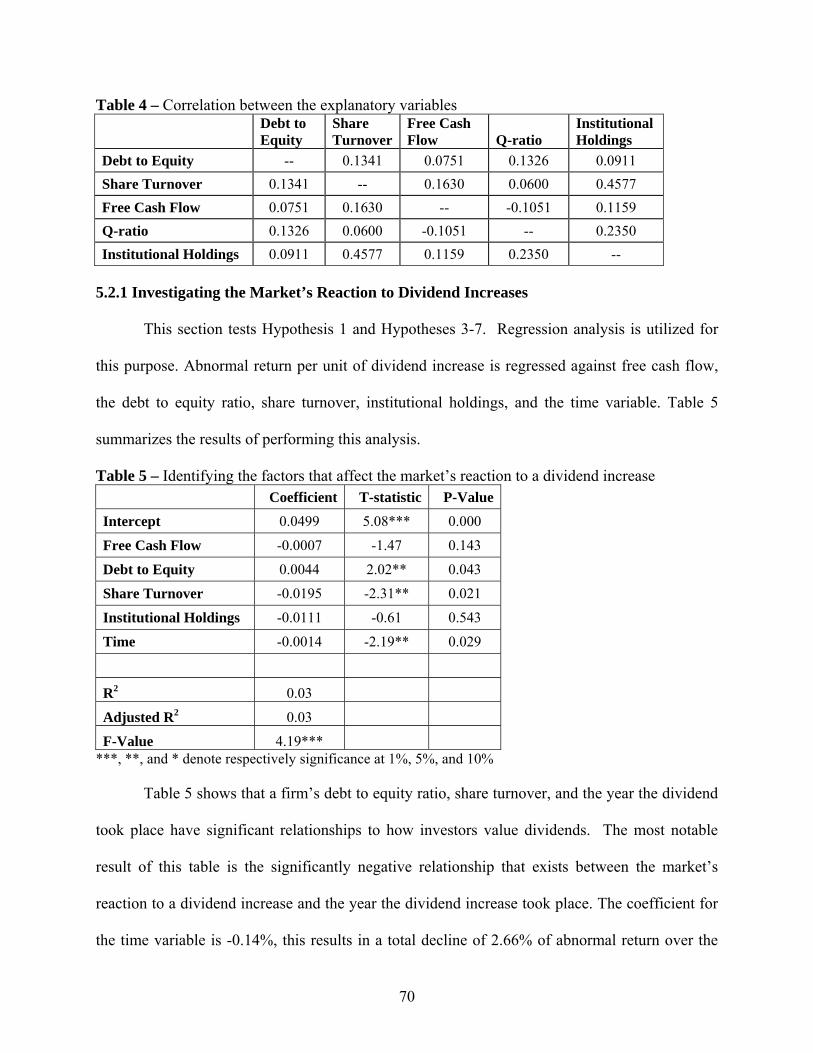
Table 4 – Correlation between the explanatory variables

Debt to Equity

Share Turnover

Free Cash Flow Q-ratio

Institutional Holdings

Debt to Equity -- 0.1341 0.0751 0.1326 0.0911 Share Turnover 0.1341 -- 0.1630 0.0600 0.4577 Free Cash Flow 0.0751 0.1630 -- -0.1051 0.1159 Q-ratio 0.1326 0.0600 -0.1051 -- 0.2350 Institutional Holdings 0.0911 0.4577 0.1159 0.2350 --

5.2.1 Investigating the Market’s Reaction to Dividend Increases

This section tests Hypothesis 1 and Hypotheses 3-7. Regression analysis is utilized for

this purpose. Abnormal return per unit of dividend increase is regressed against free cash flow,

the debt to equity ratio, share turnover, institutional holdings, and the time variable. Table 5

summarizes the results of performing this analysis.

Table 5 – Identifying the factors that affect the market’s reaction to a dividend increase Coefficient T-statistic P-Value

Intercept 0.0499 5.08*** 0.000

Free Cash Flow -0.0007 -1.47 0.143

Debt to Equity 0.0044 2.02** 0.043

Share Turnover -0.0195 -2.31** 0.021

Institutional Holdings -0.0111 -0.61 0.543

Time -0.0014 -2.19** 0.029

R2 0.03

Adjusted R2 0.03

F-Value 4.19*** ***, **, and * denote respectively significance at 1%, 5%, and 10% Table 5 shows that a firm’s debt to equity ratio, share turnover, and the year the dividend

took place have significant relationships to how investors value dividends. The most notable

result of this table is the significantly negative relationship that exists between the market’s

reaction to a dividend increase and the year the dividend increase took place. The coefficient for

the time variable is -0.14%, this results in a total decline of 2.66% of abnormal return over the

70

entire sample. This is important as it provides evidence that the market does not concern itself

with dividend increases, and hence dividends, as much as it once did. It is not surprising to find

this as Fama and French (2001) documented that firms have a lower propensity to pay dividends.

Combining their results with those found here imply that a firm’s decreased propensity to pay

dividends may be the result of a change in investor demand. Some of the possible reasons as to

why this pattern is found may be the improvements in corporate governance, more timely

releases of company information, and more efficient methods of distributing profits. These

changes may mean that dividends are no longer needed to signal a firm’s quality or to reduce its

agency costs.

Now turning the examination to the other variables there are a number of interesting

observations. The first is that the slope coefficient on the debt to equity ratio is significantly

positive, when it was expected to be negative. It was thought to be negative as dividends and

interest payments both reduce the potential agency costs of a firm. Thus, if a firm has large

interest payments, the increased dividend payment would be redundant as Jensen (1986) points

out. What a positive coefficient suggests is that investors value dividends more for firms that

have high debt loads. The most logical explanation for this, and previously not expressed in the

literature, is that interest payments place cash flow constraints on a firm; and a firm that raises its

dividend in spite of its already constrained cash flow is signalling to the market that it expects

future cash flows to be high enough to maintain both the current debt load and the increased

dividend stream. This suggestion supports the signalling theory at the expense of agency theory.

A firm’s common share turnover is significantly negative. This is the first time that an

attempt has been made to see if the market reacts differently to firms with different liquidity

levels. This is important as it should be easier to sell stock (and thus the process of making a

71

homemade dividend is easier) when a firm is more liquid. The evidence from Table 5 shows this

is true as the higher a firm’s common share turnover, the lower the market’s reaction to a

dividend increase. The advantage to investors of being able to create their own dividend is that it

allows the investor to time their consumption decisions and tax liabilities; whereas dividends

force both of these events unilaterally on all shareholders.

The coefficients of institutional holdings and free cash flow measures are both negative

but statistically insignificant. In particular, it is surprising to see that the free cash flow measure

is negative when agency theory predicts it should be positive. If it was significant, it may

contradict the conclusions of Lang and Litzenberger (1989). They suggest that a firm with

substantial free cash flows will have tendency to over-invest by accepting marginal investment

projects while increases in dividend payments will reduce the ability of managers to invest in

such projects. Therefore, a dividend increase by a firm that has a high level of free cash flow

should have a positive effect on share prices. As a result, further investigation is warranted.

It is important to remember that Lang and Litzenberger (1989) never computed a firm’s

free cash flow. They made their conclusions about a firm’s free cash flow by looking at the

relation between dividend increases and the firm’s q-ratio. They tested to see if there was a

statistically significant difference between firms whose q-ratios were greater than and less than

one. They found that firms with q-ratios less than one had a statistically significant larger

reaction to dividend increases. They concluded from this that firms with larger free cash flows

(and hence greater agency costs) have greater responses to dividend changes. While it is

possible that a relationship may exist between a firm’s q-ratio and its free cash flows, it is

important to point out that free cash flows were never calculated in Lang and Litzenberger’s

(1989) study. What if the assumption that the relationship between free cash flows and agency

72

costs that they postulate is not true? It is more appropriate to calculate the free cash flows of a

firm and then test for the relationship. It is also important to recognize that the q-ratio

traditionally measures a firm’s growth prospects, not its agency conflicts.

In order to see if there is any correlation between free cash flows and the q-ratios for the

firms in this sample their correlation coefficient was calculated. The result of this was surprising

as the correlation was only 0.01466, which essentially means that there isn’t any correlation. In

order to test the robustness of this number I gathered the q-ratios and free cash flows for all of

the firms who declared a dividend in 2004 and calculated the correlation coefficient for this

second sample. This ended up being –0.00261 which confirms that the correlation between a

firm’s q-ratio and free cash flows is negligible. This means that the assumption that a

relationship between free cash flows and q-ratios is not warranted.

In order to see if my sample is similar to Lang and Litzenberger’s (1989) in that those

firms’ whose q-ratios are less than one have greater responses to increases in dividends a

difference of means test was used. The results show that firms with q-ratios less than one had a

significantly larger reaction to dividend increases. The t-statistic for this test is 2.08 which is

statistically significant at the 5% level. This means that my sample has the similar characteristic

to Lang and Litzenberger’s (1989) in that firms with q-ratios less than one have a greater market

response to an increase in dividends.

The fact that I get the same results as Lang and Litzenberger (1989), that q-ratios have

essentially no correlation with free cash flows, and that a previous study by Lie10 (2000) found

no relationship between abnormal returns (not abnormal returns per unit of dividend increase)

and his measure of ‘undistributed cash flow’ (not free cash flow per share), gives rise to the

10 For a full comparison of Lie’s (2000) measure and the one used in this thesis please refer to section 4.2

73

possibility that a negative relationship may exist between free cash flows of a firm and its

dividend. This possibility is further examined in the next sub-section.

5.2.2 Exploring Other Measures of Free Cash Flow

As the proposed free cash flow measure is cumbersome to calculate and relies on many

inputs, it may be possible that investors use a different or simpler measure to estimate potential

agency costs. For this reason, I repeat the same analysis by using different measures of free cash

flows. First, I repeat the analysis using lagged free cash flows. This is the same measure of free

cash flows used previously except it is lagged by one year. A lag is important as investors may

be dealing with old or stagnant information, and the lag allows for information to be incorporated

fully. Old information may be relevant to the decision makers’ reactions as the majority of

dividend increases coincide with a firm’s fiscal year end, and the current financial statements are

not available generally for three months. It can be argued that the lag isn’t necessary for the other

variables (and illustrated later in this chapter in section 5.3) as they are much simpler to estimate

because they have fewer inputs. Second, I use operating cash flows as the proxy for free cash

flows. This is a simple measure as it is reported in the financial statements. This measure of cash

flows may be more relevant as it is often considered the firm’s sustainable cash flow. Third, I use

cash plus cash equivalents as a simple measure of the potential agency costs. This may be

relevant as it measures the amount of cash that a manager can mismanage without having to raise

any more capital or earn any more profits. The final measure is taking the original measure of

free cash flow per share and then dividing it by share price. This final measure incorporates the

possibility that free cash flows are priced in the market, and thus the relationship can be better

seen between dividends and cash flows once they are priced accordingly.

74

The same regression equation that is used to generate Table 5 is used in this analysis.

Only the free cash flow variable changes. In an additional step, I add to the equation a dummy

variable for the q-ratio. This dummy variable takes the value of 1 if the firm’s q-ratio is greater

than one and 0 otherwise. The q-ratio is added as a dichotomous variable rather than a

continuous one in order to be consistent with the work of Land and Litzenberger (1989). In

section 5.3 (a section that discusses other model specifications) it is analyzed as a continuous

variable. The q-ratio is added because it was shown in the difference of means test that there

was a significantly different response to an increase to a dividend depending on the firm’s q-

ratio. It is important to see if this relationship holds when the other variables are included.

Table 6 shows that the different proxies for free cash flow produce results consistent with

the findings reported in Table 5. Specifically the coefficients are negative for the new free cash

flow variables. In addition, they are significant at the 10% and 5% levels for the lagged free cash

flows and for the cash and cash equivalents measure respectively. While the significance of the

free cash flow measures can be debated as its significance depends on which measure is used, it

is clear from Tables 5 and 6 that the evidence does not support the theoretical relationships that

agency theory predicts. On the contrary, evidence presented in these tables seems to contradict

the proposition that dividend increases should reduce the potential for agency conflicts.

75

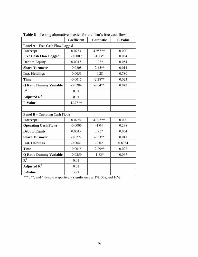
Table 6 – Testing alternative proxies for the firm’s free cash flow Coefficient T-statistic P-Value

Panel A – Free Cash Flow Lagged Intercept 0.0753 4.95*** 0.000 Free Cash Flow Lagged -0.0009 -1.73* 0.084

Debt to Equity 0.0047 1.93* 0.054

Share Turnover -0.0208 -2.45** 0.014

Inst. Holdings -0.0053 -0.28 0.780

Time -0.0015 -2.28** 0.023

Q Ratio Dummy Variable -0.0284 -2.04** 0.042

R2 0.01

Adjusted R2 0.01

F-Value 4.37***

Panel B – Operating Cash Flows Intercept 0.0755 4.77*** 0.000 Operating Cash Flows -0.0006 -1.04 0.298

Debt to Equity 0.0045 1.93* 0.054

Share Turnover -0.0222 -2.53** 0.011

Inst. Holdings -0.0041 -0.02 0.8334

Time -0.0015 -2.29** 0.022

Q Ratio Dummy Variable -0.0259 -1.83* 0.067

R2 0.01

Adjusted R2 0.01

F-Value 3.91 ***, **, and * denote respectively significance at 1%, 5%, and 10%

76

Table 6 (Continued) – Testing alternative proxies for the firm’s free cash flow Coefficient T-statistic P-Value Panel C – Cash and Cash Equivalents

Intercept 0.0771 5.13*** 0.000 Cash and Cash Equivalents -0.0002 -1.96* 0.050

Debt to Equity 0.0039 1.85** 0.028

Share Turnover -0.0215 -2.54** 0.011

Inst. Holdings -0.0058 -0.31 0.757

Time -0.0014 -2.2** 0.028

Q Ratio Dummy Variable -0.0278 -2.18** 0.029

R2 0.01

Adjusted R2 0.01

F-Value 4.52

Panel D – FCF per share divided by Share Price

Intercept 0.0729 4.91*** 0.000 FCF per Share / Share Price -2.8963 -1.26 0.209

Debt to Equity 0.0027 1.27 0.205

Share Turnover -0.0243 -2.88** 0.004

Inst. Holdings -0.0021 -0.011 0.911

Time -0.0014 -2.08** 0.038

Q Ratio Dummy Variable -0.0298 -2.19* 0.028

R2 0.01

Adjusted R2 0.01

F-Value 3.91 ***, **, and * denote respectively significance at 1%, 5%, and 10% Another important insight gained from Table 6 is that the q-ratio is negative and

significantly different from zero. This means that those firms whose q-ratios are less than one

have larger reactions to dividend increases. This confirms the difference of means test and the

results of Lang and Litzenberger (1989). A possible interpretation of this result is that investors

interpret a dividend increase from a firm that has low investment prospects (as measured by a q-

77

ratio of less than one) as a signal of future performance, and this signal is in spite of the market’s

low expectations. If this is correct, undervalued firms could use this to their advantage by

signalling their future prospects and thereby increase their value by increasing their dividend.

5.3 Other Model Specifications

A potential critique of all the results so far may be that the R2 measures are small. While

this is true, the R2 reported in Tables 5 and 6 are similar in scale to those reported by other

studies that have examined abnormal returns surrounding dividend changes. For example Lie

(2000) reports having an adjusted R2 of 0.04 for the two regressions he ran on his dividend

initiation sample. It is also important to remember that the chance of finding significant

variables by chance with such small R2 values is extremely low which decreases the likelihood of

finding spurious relationships. The purpose of this section is to test whether different model

specifications can increase the R2 values.

It is also important to look at the economic significance of these variables, just not the

statistical significance. The coefficients on the variables are quite small. Remembering that by

definition an abnormal return over one day is small, then it is not surprising that the coefficients

describing it are of the same magnitude.

Examining the issues of multicollinearity will also be explored further here. In particular

is the concern that the institutional ownership variable is highly correlated with other variables

but does not appear to be significantly related to the dependent variable.

5.3.1 Multicollinearity

In order to deal with multicollinearity two methods will be chosen. First, the institutional

variable will be dropped from the regression equation. If multicollinearity is a problem and an

offending variable is dropped, then it is expected that there will be a dramatic shift in the

78

interpretation of the variables such as a variable changing its sign. The second method to deal

with multicollinearity is to regress institutional ownership on the dependent variable (abnormal

return/percentage increase in dividend), and then include the residual from the fitted relationship

and observation as a proxy for institutional ownership. This leaves a variable that is related to

institutional ownership and unrelated to the other independent variables

Table 7 Panel A shows the results of excluding the institutional holdings variable, Panel

B shows the results of replacing the institutional holdings variable with the residual just

described.

79

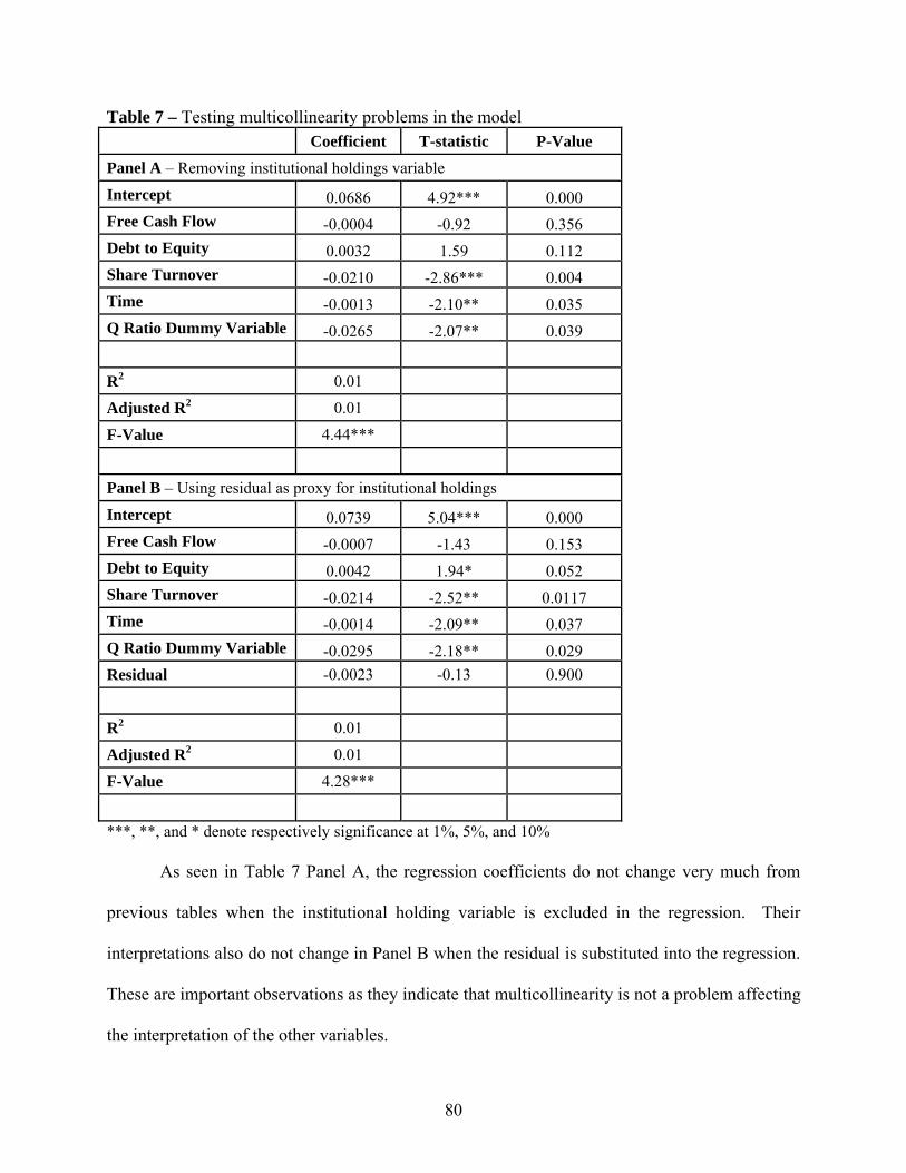
Table 7 – Testing multicollinearity problems in the model Coefficient T-statistic P-Value Panel A – Removing institutional holdings variable

Intercept 0.0686 4.92*** 0.000 Free Cash Flow -0.0004 -0.92 0.356 Debt to Equity 0.0032 1.59 0.112 Share Turnover -0.0210 -2.86*** 0.004 Time -0.0013 -2.10** 0.035 Q Ratio Dummy Variable -0.0265 -2.07** 0.039

R2 0.01

Adjusted R2 0.01

F-Value 4.44***

Panel B – Using residual as proxy for institutional holdings

Intercept 0.0739 5.04*** 0.000 Free Cash Flow -0.0007 -1.43 0.153 Debt to Equity 0.0042 1.94* 0.052 Share Turnover -0.0214 -2.52** 0.0117 Time -0.0014 -2.09** 0.037 Q Ratio Dummy Variable -0.0295 -2.18** 0.029 Residual -0.0023 -0.13 0.900

R2 0.01

Adjusted R2 0.01

F-Value 4.28***

***, **, and * denote respectively significance at 1%, 5%, and 10% As seen in Table 7 Panel A, the regression coefficients do not change very much from

previous tables when the institutional holding variable is excluded in the regression. Their

interpretations also do not change in Panel B when the residual is substituted into the regression.

These are important observations as they indicate that multicollinearity is not a problem affecting

the interpretation of the other variables.

80

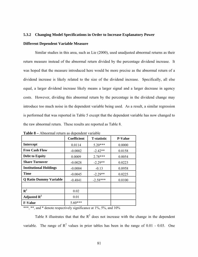
5.3.2 Changing Model Specifications in Order to Increase Explanatory Power

Different Dependent Variable Measure

Similar studies in this area, such as Lie (2000), used unadjusted abnormal returns as their

return measure instead of the abnormal return divided by the percentage dividend increase. It

was hoped that the measure introduced here would be more precise as the abnormal return of a

dividend increase is likely related to the size of the dividend increase. Specifically, all else

equal, a larger dividend increase likely means a larger signal and a larger decrease in agency

costs. However, dividing this abnormal return by the percentage in the dividend change may

introduce too much noise in the dependent variable being used. As a result, a similar regression

is performed that was reported in Table 5 except that the dependent variable has now changed to

the raw abnormal return. These results are reported as Table 8.

Table 8 – Abnormal return as dependent variable Coefficient T-statistic P-Value Intercept 0.0114 5.20*** 0.0000 Free Cash Flow -0.0002 -2.42** 0.0158 Debt to Equity 0.0009 2.78*** 0.0054 Share Turnover -0.0028 -2.29** 0.0223 Institutional Holdings -0.0004 -0.13 0.8958 Time -0.0045 -2.29** 0.0225 Q Ratio Dummy Variable -0.4841 -2.58*** 0.0100

R2 0.02 Adjusted R2 0.01

F-Value 5.60*** ***, **, and * denote respectively significance at 1%, 5%, and 10% Table 8 illustrates that that the R2 does not increase with the change in the dependent

variable. The range of R2 values in prior tables has been in the range of 0.01 - 0.03. One

81

variable of interest in this table is the free cash flow measure, which is now significant when it

was not in Table 5. This provides more support for the possibility of the free cash flow measure

having a statistically significant negative relationship.

Abnormal Trading Volume

Michaely, Thaler, and Womack (1995) studied the market reaction to events of dividend

initiations and omissions. They argue that volume changes around these events indicate that investors are

shifting in or out of a stock that experienced a change. Thus, abnormal volume surrounding dividend

initiations and omissions is an indication of clientele effects. Consistent with Michaely, Thaler, and

Womack (1995), an additional variable that measures the abnormal volume changes surrounding

the dividend increase date is included in the regressions. The volume measure that is described in

section 4.2 for the different time periods is used for this purpose. It is hoped that the additional

information that the market provides with the change in volume will increase the explanatory

power of the model while preserving the conclusions related to the other variables. The results

of these regressions are presented in Table 9.

82

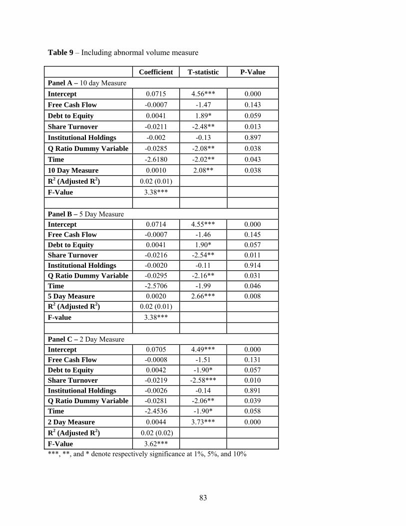
Table 9 – Including abnormal volume measure

Coefficient T-statistic P-Value Panel A – 10 day Measure Intercept 0.0715 4.56*** 0.000 Free Cash Flow -0.0007 -1.47 0.143 Debt to Equity 0.0041 1.89* 0.059 Share Turnover -0.0211 -2.48** 0.013 Institutional Holdings -0.002 -0.13 0.897 Q Ratio Dummy Variable -0.0285 -2.08** 0.038 Time -2.6180 -2.02** 0.043 10 Day Measure 0.0010 2.08** 0.038 R2 (Adjusted R2) 0.02 (0.01) F-Value 3.38*** Panel B – 5 Day Measure Intercept 0.0714 4.55*** 0.000 Free Cash Flow -0.0007 -1.46 0.145 Debt to Equity 0.0041 1.90* 0.057 Share Turnover -0.0216 -2.54** 0.011 Institutional Holdings -0.0020 -0.11 0.914 Q Ratio Dummy Variable -0.0295 -2.16** 0.031 Time -2.5706 -1.99 0.046 5 Day Measure 0.0020 2.66*** 0.008 R2 (Adjusted R2) 0.02 (0.01) F-value 3.38*** Panel C – 2 Day Measure Intercept 0.0705 4.49*** 0.000 Free Cash Flow -0.0008 -1.51 0.131 Debt to Equity 0.0042 -1.90* 0.057 Share Turnover -0.0219 -2.58*** 0.010 Institutional Holdings -0.0026 -0.14 0.891 Q Ratio Dummy Variable -0.0281 -2.06** 0.039 Time -2.4536 -1.90* 0.058 2 Day Measure 0.0044 3.73*** 0.000 R2 (Adjusted R2) 0.02 (0.02) F-Value 3.62*** ***, **, and * denote respectively significance at 1%, 5%, and 10%

83

Table 9 illustrates that the change in volume variable is significant for all three time

periods and the related t-statistic is increasing with shorter time periods. In addition, the

explanatory power of the model increases marginally with the additional variable. This evidence

shows that there is a relationship between volume changes and dividend increases and that the

effects of the volume change is detectable for at least 10 days following the dividend increase.

Note that Michaely et al. (1995) did not find significant changes in volume when they

looked at firms who initiated or omitted a dividend. The analysis here shows that the market

reaction to announcements of dividend increases is positively affected by the changes in volume

following the announcement. This provides some evidence that there might be some dividend

clientele shifting. Yet, a full analysis of volume changes surrounding dividend increases is

needed to confirm the existence of clientele effects.

Table 9 also shows that the conclusions regarding the other independent variables do not

change with the inclusion of the change in volume variable.

Lagged Values and Percentage Increases in Variables

Another way to try to increase the R2 of the regressions is to alter the definitions of the

variables. The first method is to use lag values of the variables, and the second method is to use

percentage increases in the variables from the previous years. The lagged model is based on the

idea that investors are using old information to include in their analysis as current year data may

not be available (also for this model the time variable is not lagged as it does not seam

appropriate to do so). The percentage increase model is based on the possibility that investors

are concerned with changes in the variables and not in their absolute levels. For this second

model, the time variable, and the q-ratio dummy variable are not lagged. The results of these

regressions are found in Table 10.

84

Table 10 – Lagged Values and Percentage Increase Values for independent variables Coefficient T-statistic P-Value

Panel A – Lagged Values

Intercept 0.1038 3.55*** 0.000 Free Cash Flow -0.0024 -2.00** 0.046 Debt to Equity 0.0065 1.48 0.180 Share Turnover -0.0144 -1.12 0.263 Institutional Holdings -0.0120 -0.21 0.838 Q Ratio Dummy Variable -0.0517 -0.76 0.447 Time -0.0015 -0.76 0.447 R2 0.01

Adjusted R2 0.01

F-Value 1.92**

Panel B – Percentage Increase

Intercept 0.1000 3.75*** 0.000 Free Cash Flow 0.0002 0.94 0.349 Debt to Equity -0.0004 -0.99 0.321 Share Turnover 0.0036 0.33 0.739 Institutional Holdings 0.0005 0.94 0.349 Q Ratio Dummy Variable -0.0591 -2.78*** 0.006 Time -0.0019 -0.98 0.328 R2 0.01

Adjusted R2 0.01

F-Value 1.91* ***, **, and * denote respectively significance at 1%, 5%, and 10% The primary aim of Table 10 was to try and increase the R2 of the regression. As seen in

this table, the R2 is not increased for either panel A or B when compared to earlier results. Also

in unreported results, the regressions were performed without including the time and the q-ratio

dummy variables, as these were not transformed. The results of these unreported models were

not materially different. As there was a time cost to gathering this data, the data was only

collected for the years 1990-1999. As the only significant t-statistic for this table is the free cash

85

flow measure in Panel A, it appears that it is more appropriate to use current year data than either

of these alternatives.

Q-ratio treated as a continuous variable

In order to try and further understand the value of the q-ratio in this modelling process, it

is now introduced as a continuous variable rather than a dichotomous one. It was originally

modelled as a dummy variable to follow the methodology of Lang and Litzenberger (1989) who

found that dividend valuation was dependent on a firm’s q-ratio being above or below unity.

Table 11 shows the results of this regression.

Table 11 – Q-ratio as a continuous variable instead of a dummy variable Coefficient T-statistic P-value

Intercept 0.0505 5.07*** 0.000

Free Cash Flow -0.0008 -1.49 0.135

Debt to Equity 0.0045 2.05** 0.040

Share Turnover -0.0197 -2.32** 0.021

Inst. Holdings -0.0095 -0.50 0.614

Time -0.0014 -2.17** 0.030

Q Ratio Continuous Variable -0.0005 -0.36 0.717

R2 0.01

Adjusted R2 0.01

F-Value 3.50*** ***, **, and * denote respectively significance at 1%, 5%, and 10%

As seen in Table 11, treating the q-ratio as a continuous variable does not materially alter

the values of the coefficients or their significance. It is important to see that while the q-ratio is

still negative, it is no longer a significant variable. This gives evidence that the relationship for

this variable is better modeled dichotomously, and that investors are more concerned with the q-

ratio’s relation to being above/below unity than its true value.

86

87

Fama-Macbeth Regression

A final model was performed using a Fama-Macbeth regression. Fama-Macbeth

regressions rely on the stability of the coefficients being tested and it was hoped that this

additional method would uphold the previous results presented throughout this chapter. The

results of the Fama-Macbeth regression are found in Table 12.

88

Table 12 – Fama-Macbeth regression results

Year Debt to Equity Share Turnover Institutional

Holdings Free Cash Flow Slope T-Stat Slope T-Stat Slope T-Stat Slope T-Stat R2 Adj. R2

1985 -0.00752 -0.46 -0.03264 -0.83 0.07798 0.10 -0.00085 -0.43 0.0248 -0.03091986 0.00796 0.26 -0.01284 -0.20 0.01602 0.13 -0.01211 -1.92** 0.0648 -0.00201987 0.00649 0.11 -0.00092 -0.01 0.13789 0.97 0.00046 0.10 0.0133 -0.03321988 0.00274 0.79 -0.00711 -0.18 -0.04020 -0.47 0.00385 1.94** 0.0420 0.05541989 -0.00003 0.00 -0.02566 -1.18 0.10532 1.80* 0.00075 0.26 0.0296 -0.00301990 -0.00589 -0.50 0.01950 0.34 -0.02118 -0.17 0.00489 1.02 0.0132 -0.03381991 0.03576 1.54 -0.01746 -0.55 -0.10952 -1.10 -0.00175 -0.35 0.0796 0.01271992 -0.00754 -0.66 0.06520 1.22 -0.17556 -1.53 0.00031 0.11 0.0458 -0.00261993 0.02259 3.01** -0.02835 -0.59 0.06332 0.67 -0.00085 -0.61 0.0942 0.05831994 -0.00191 -0.09 -0.02702 -0.82 -0.04835 -0.64 0.00214 0.47 0.0112 -0.18301995 -0.02804 -1.29 0.04380 1.62 -0.07396 -1.39 0.00100 0.40 0.0342 0.00471996 -0.00645 -0.47 -0.00540 -0.22 -0.03366 -0.54 -0.00151 -0.82 0.0161 -0.01321997 0.00886 0.44 0.00659 0.11 0.11510 0.16 -0.00451 -1.04 0.0153 -0.02411998 0.05331 2.38** -0.02332 -0.44 0.11418 1.46 -0.00512 -1.34 0.0646 0.02721999 -0.00063 -0.02 -0.05329 -0.50 -0.02806 -0.20 -0.00142 -0.42 0.0166 -0.04592000 -0.01504 -0.69 0.02921 0.37 -0.05864 -0.41 -0.00029 -0.05 0.0095 -0.04632001 0.01701 1.59 0.03368 0.69 -0.03597 -0.49 0.00729 1.22 0.0740 0.01332002 -0.00870 -0.77 -0.07192 -1.68 0.06935 0.65 0.00285 0.69 0.0593 0.00402003 0.00728 1.58 0.00393 0.20 -0.01577 -0.32 -0.00202 0.00 0.0327 -0.00252004 0.00329 0.52 -0.09565 2.98** -0.01614 -0.19 0.00091 0.78 0.1808 0.1460

Average 0.00418 -0.00998 0.00211 -0.00030 Std. Dev. 0.01793 0.03847 0.08313 0.00405 T- Stat 0.2330 -0.2595 0.0254 -0.0737

***, **, and * denote respectively significance at 1%, 5%, and 10%

89

As Table 12 shows, not much can be garnered from the Fama-Macbeth regression. The

Fama-Macbeth coefficients (reported as the average in Table 10) are not significant for any of

the variables tested. It is easy to see why they are not significant as the Fama-Macbeth

coefficients depend on stability, and the coefficients presented in Table 10 are not stable through

the years and they often switch between being positive and negative.

5.4 The Impact of Market Conditions on the Reaction to Dividend Increases.

From 1983 to 2000 the stock market was in a bull market that some consider it to be the

strongest one that the United States has ever seen. There were a few market drops along the way

such as what has become known as Black Monday in October 1987 and the currency crises of

the late 1990s. However, neither of these events caused too much disruption as the stock market

increased on an annual basis for each calendar year during this time period. The decline that

started in 2000 was different though as the market finished lower that year, and it closed at lower

levels in both 2001 and 2002. It is possible that entering a bear market from such a prolonged

bull market may affect the way the market reacts to a dividend increase.

In order to test this, the results of equation 10 (with the q-ratio dummy variable added as

it has been shown to be significant) are presented in Table 13.

89

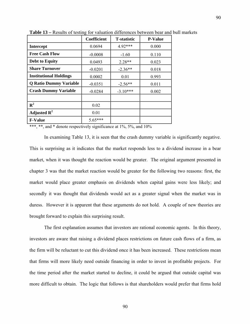
90

Table 13 – Results of testing for valuation differences between bear and bull markets Coefficient T-statistic P-Value Intercept 0.0694 4.92*** 0.000

Free Cash Flow -0.0008 -1.60 0.110 Debt to Equity 0.0493 2.28** 0.023 Share Turnover -0.0201 -2.36** 0.018 Institutional Holdings 0.0002 0.01 0.993 Q Ratio Dummy Variable -0.0351 -2.56** 0.011 Crash Dummy Variable -0.0284 -3.10*** 0.002 R2 0.02

Adjusted R2 0.01

F-Value 5.65*** ***, **, and * denote respectively significance at 1%, 5%, and 10% In examining Table 13, it is seen that the crash dummy variable is significantly negative.

This is surprising as it indicates that the market responds less to a dividend increase in a bear

market, when it was thought the reaction would be greater. The original argument presented in

chapter 3 was that the market reaction would be greater for the following two reasons: first, the

market would place greater emphasis on dividends when capital gains were less likely; and

secondly it was thought that dividends would act as a greater signal when the market was in

duress. However it is apparent that these arguments do not hold. A couple of new theories are

brought forward to explain this surprising result.

The first explanation assumes that investors are rational economic agents. In this theory,

investors are aware that raising a dividend places restrictions on future cash flows of a firm, as

the firm will be reluctant to cut this dividend once it has been increased. These restrictions mean

that firms will more likely need outside financing in order to invest in profitable projects. For

the time period after the market started to decline, it could be argued that outside capital was

more difficult to obtain. The logic that follows is that shareholders would prefer that firms hold

90

91

on to cash during times when capital is scarce, as the firm may need the capital more than

shareholders need the dividend. This possibility is interesting because it actually goes against

what agency theory would predict as it illustrates a situation where shareholders are willing to

increase the amount of cash a firm has, and therefore its potential agency conflicts.

The second explanation relies on behavioural finance, specifically the theory proposed by

Thaler (1983) and discussed in detail in section 2.4. In this theory, Thaler (1983) proposes that

dividends are treated as a silver lining in periods of market decline, and treated as an added

bonus during periods of market strength. If one subscribes to this theory, then Table 13 shows

that the added bonus is worth more than the silver lining

Seeing that a change in market reaction occurs when the sample is divided up between

those events that took place before and after the year 2000, another set of regressions is

performed in order to see if the firm specific factors (thus ignoring the crash dummy and the year

the dividend took place) are different between these two time periods. Table 14 shows the

results of these regressions.

91

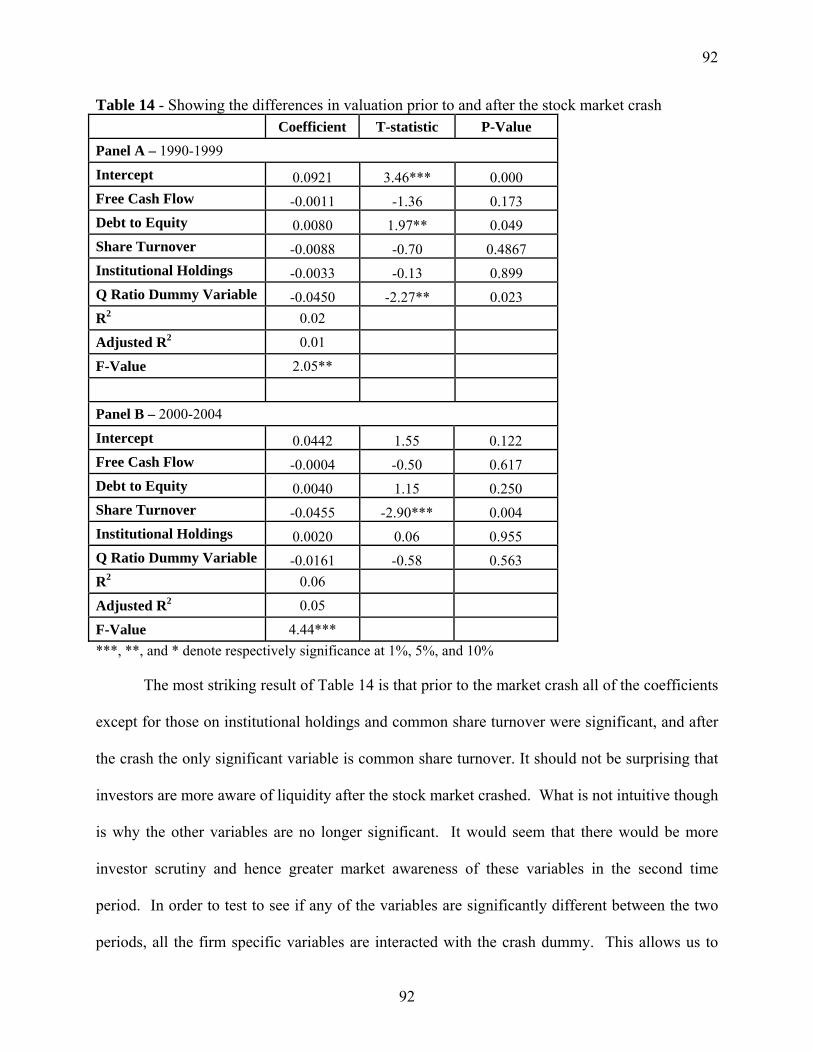
92

Table 14 - Showing the differences in valuation prior to and after the stock market crash Coefficient T-statistic P-Value

Panel A – 1990-1999

Intercept 0.0921 3.46*** 0.000 Free Cash Flow -0.0011 -1.36 0.173 Debt to Equity 0.0080 1.97** 0.049 Share Turnover -0.0088 -0.70 0.4867 Institutional Holdings -0.0033 -0.13 0.899 Q Ratio Dummy Variable -0.0450 -2.27** 0.023 R2 0.02

Adjusted R2 0.01

F-Value 2.05**

Panel B – 2000-2004

Intercept 0.0442 1.55 0.122 Free Cash Flow -0.0004 -0.50 0.617 Debt to Equity 0.0040 1.15 0.250 Share Turnover -0.0455 -2.90*** 0.004 Institutional Holdings 0.0020 0.06 0.955 Q Ratio Dummy Variable -0.0161 -0.58 0.563 R2 0.06

Adjusted R2 0.05

F-Value 4.44*** ***, **, and * denote respectively significance at 1%, 5%, and 10% The most striking result of Table 14 is that prior to the market crash all of the coefficients

except for those on institutional holdings and common share turnover were significant, and after

the crash the only significant variable is common share turnover. It should not be surprising that

investors are more aware of liquidity after the stock market crashed. What is not intuitive though

is why the other variables are no longer significant. It would seem that there would be more

investor scrutiny and hence greater market awareness of these variables in the second time

period. In order to test to see if any of the variables are significantly different between the two

periods, all the firm specific variables are interacted with the crash dummy. This allows us to

92

93

draw specific conclusions about the differences that exist between the two time periods. These

results are found in Table 15.

Table 15 – Identifying factors that are different after the market crash Coefficient T-statistic P-Value

Intercept 0.0767 4.00*** 0.000

Debt to Equity 0.0063 2.07** 0.039

Free Cash Flow -0.0014 -2.14** 0.032

Inst. Holdings 0.0054 0.25 0.802

Share Turnover -0.0079 -0.79 0.432

Q-ratio Dummy -0.0401 -2.55** 0.011

Crash Dummy -0.0167 -0.44 0.658

Crash * Debt to Equity -0.0042 -0.82 0.413

Crash * Share Turnover -0.0426 -2.07** 0.039

Crash * Inst. Holdings -0.0010 -0.02 0.983

Crash * Free Cash Flow 0.0017 1.44 0.149

Crash * Q-ratio Dummy 0.0232 0.64 0.522 R2 0.06

Adjusted R2 0.05

F-Value 3.73*** ***, **, and * denote respectively significance at 1%, 5%, and 10% Table 15 is interesting in that it shows that the liquidity measure, common share turnover,

is not significant for the whole sample (as seen by not having a significant coefficient on the base

variable) but it is after the market crash as evidenced by its significance when interacted with the

crash dummy variable. As stated earlier, it is intuitive to understand why investors would pay

more attention to liquidity after the stock market started to decline as positions may need to be

sold quickly.

It is also interesting in this regression to see that the coefficients for the debt to equity and

free cash flow are significant for the whole sample which is once again opposite to what agency

93

94

theory predicts. This provides more evidence that investors are not concerned with the potential

agency costs of dividends as discussed in section 5.3.

As it has been shown that the market reacts differently to a dividend increase depending

on the time period it took place in, it is worthwhile to look at the descriptive statistics of the

independent variables for each time period. Table 16 shows the means for the two time periods,

and it also reports the t-statistic from the standard difference of means test.

Table 16 – Summary statistics for the time periods 1990-1999 and 2001-2004 1990-1999 2001-2004

Mean Std. Dev. Mean Std. Dev. Difference of means T-stat. P-value

Debt to Equity 0.600 0.798 0.999 1.269 5.51*** 0.000

Share Turnover 0.609 0.409 0.788 0.592 5.24*** 0.000

Free Cash Flow 2.292 4.386 4.044 7.927 3.93*** 0.000

Q-ratio 2.275 1.601 3.059 2.55 5.39*** 0.000

Institutional Holdings 0.431 0.213 0.486 0.255 3.57*** 0.000 ***, **, and * denote respectively significance at 1%, 5%, and 10% Table 16 shows that all of the variables are larger in the second time period. This is

interesting as it may indicate that there was a shift in the firms who increased their dividend.

Particularly, larger values of these variables indicate larger and more established firms. For

example, it is common knowledge that more established firms attract more institutional

ownership. In order to test the possibility that only larger firms increased their dividend in the

second time period three different measures of size are gathered and then tested for using a

difference of means test. The three size measures gathered are market value of equity, total

assets, and sales. Different measures are gathered in order to ensure that the results are not

biased according to the definition of firm size. These results are found in Table 17.

94

95

Table 17 – Examining the size of the firms for the time periods 1990-1999 and 2001-2004 1990-1999 2001-2004

Mean Std. Dev. Mean Std. Dev. Difference of

means T - stat. P-value

Sales 4269 11804 5281 13996 1.23 0.210

Market Value 5475 14734 11337 37077 2.95*** 0.003

Total Assets 10218 37227 25469 35409 2.54** 0.011 ***, **, and * denote respectively significance at 1%, 5%, and 10% The figures reported in Table 17 are in millions of dollars. The total assets and market

value measures for firm size indicate that firms were larger in the second time period when

compared to the first. This is important because large firms broadly speaking have a larger

shareholder base and a larger analyst following. These facts result in more information being

known about larger firms. As a result, the signalling theory of dividends would predict the

smaller market reaction in the second time period as these firms have less to signal.

For both Tables 16 and 17, the result of being larger in the second time period could be

the result of inflationary type pressures on these variables. As a result first time period was

reduced to the years 1995-1999 and the analysis was repeated. In unreported results, shortening

the time frame in the first period does not alter the significance of any of the variables in either

Tables 16 and 17.

95

96

CHAPTER 6

SUMMARY FINDINGS AND FUTURE RESEARCH

Section 6.1 summarizes the findings of this thesis. The most important results were that

evidence is found that the market reaction to a dividend increase is a decreasing function of time,

and that this reaction is smaller in a bear market when compared to a bull market. In addition,

the market reaction to a dividend increase is smaller for firms who have large free cash flows and

greater liquidity while firms with high debt to equity ratios have larger reactions.

Section 6.2 discusses the directions for future research. These include exploring the

market reaction to share repurchases and further exploring the signalling theory of dividends as

evidence found in this study contradicts the predictions of agency theory.

96

97

6.1 Summary of the Findings

The following is a list of findings that were presented in this thesis as related to the stated

hypothesis in chapter 3.

1) There is evidence that the market reaction to dividend increase has weakened over the

period from 1984-2003. This is important as it is the first time in the literature that

such a relationship has been documented. This result is most likely as a result of

improved corporate governance, better and more timely financial statements, and

more efficient methods of making distributions to shareholders (ie share repurchases).

This means that the first hypothesis can be confirmed.

2) The market reaction to dividend increases is larger in bull markets than in bear

markets. This is a surprising result as it was expected that the market’s reaction

would be greater in times when capital gain returns were more uncertain. A possible

reason for this finding is that investors know that dividends place cash flow

constraints on a firm as they are rarely cut or decreased by management. Knowing

this, investors might rather have management hold on to the cash during difficult

economic times as the capital might be needed to stay solvent or invest in positive

NPV projects. This illustrates a possibility where investors want to increase the

amount of cash available to managers, which contradicts the predictions of agency

theory. Another possible reason is that larger firms increased their dividend in the

second time period, and larger firms are less likely to need the signals that dividends

may provide.

3) The third hypothesis stated that institutional ownership should play an important

factor in dividend valuation because it should reduce agency costs and act as a signal

97

98

of firm quality, both of which are hypothetical functions of dividends. What was

found is that institutional ownership does not play a role in how the market reacts to a

dividend increase. In all time periods and in any partition of the sample I was not

able to find any relationship between institutional holdings and dividends.

4) The debt to equity relationship was found to be positive, when agency theory predicts

that it should be negative. It was expected to be negative because Jensen (1986)

stated that interest payments would discipline management’s spending similarly to

dividend payments, and thus agency costs would already be reduced for firms that

have high debt levels. What was found instead was that firms with high debt levels

have dividends valued greater than firms with low debt levels. It is proposed that the

positive relationship exists because investors interpret an increase in dividends to

firms with high debt levels as a signal that the firm’s cash flows are stable and large

enough to maintain the higher dividend level indefinitely.

5) The fifth hypothesis tested in this thesis was in regards to a firm’s free cash flows and

its dividend policy. The agency theory of dividends proposes that the greater the free

cash flows of a firm, the greater the market should react to a dividend increase as this

increase would decrease the potential amount of agency conflicts. Rather than

finding this, a significantly negative relationship was found to exist depending on the

proxy used to measure free cash flows. The original measure of free cash flow as

described in section 4.2 was found to be insignificant over the entire time period as

reported in Table 4, but the lagged measure of free cash flow and the cash and cash

equivalents measure were found to be significant in Table 5. In section 5.4 (which

focused on testing for differences in valuation before and after the market crash)

98

99

Table 12 shows that the free cash flow measure was significant for the time period

1990-1999, and it was found to be significant in its base level in Table 13 after all the

variables were interacted with the crash dummy variable. This evidence leads to the

conclusion that agency theory does not hold, and in fact (similar to the debt to equity

relationship) there is evidence to support that the opposite relationship is true. Even

if one does not feel that the relationship is statistically significant (as significance is

dependent on the time period and the proxy chosen) there is no evidence to support

the hypothesized relationship between free cash flows and dividends.

6) A firm’s liquidity is an important factor in how the market reacts to an increase in

dividends. In addition, it becomes increasingly more important after the stock market

started to decline. This confirms the sixth hypothesis, which states that firms with

higher liquidity have less to gain from dividend increases.

7) The seventh hypothesis was confirmed. It means that the market’s reaction to a

dividend increase is more pronounced for firms whose q-ratio is less than one. This

confirms the earlier work of Lang and Litzenberger (1989) as they also found this

relationship. They assumed that firms with q-ratios less than unity (or less than one)

were firms with high levels of free cash flows. From this they concluded that

dividends were valued because they reduced agency problems. What was found in

this study was that q-ratios had no correlation with the free cash flow measure, thus

their assumption about free cash flows and q-ratios seems unfounded. Also, the

relationships that agency theory predicts between the market’s reaction to an increase

to dividend and free cash flows & debt do not hold; and there is some evidence that

the opposite relationship holds. With this information, it is most likely that the results

99

100

observed in regards to a firm’s q-ratio are caused by the market interpreting the

increased dividend to mean that these firms have better investment prospects than

they were originally thought to have.

8) The final hypothesis tested was in regards to the changes in volume that occur around

the dividend change. Michaely, Thaler, and Womack (1995) investigate volume

changes surrounding dividend omissions and initiations and were not able to find any

significant increases in volume. They did this in hopes to find evidence that there

was change in dividend clientele by noticing a change in volume. The data presented

here shows that the market reaction to dividend increases is positively related to the

changes in volume over periods of 2, 5, and 10 days after the dividend increase. This

may be the result of the firm changing its dividend clientele as Michaely et al. (1995)

proposed.

6.2 Future Research

Future research into this area might focus on trying to determine if the market’s reaction

to share repurchases has also changed over a similar time period. If it is shown that the market

reacts more now than it once did, then a payout substitution theory could be presented which

would state that market has increased its desire for share repurchases at the expense of dividends.

This theory would give evidence that the declining propensity of firms to pay a dividend is a

result of changing investor tastes.

It would also be important to test whether firms that have high debt levels are signalling

to the market about their future performance by increasing their dividends. It is proposed from

the fact that the debt to equity coefficient has the opposite relationship that agency theory

predicts, that the market may interpret a dividend increase from firms with high debt levels as a

100

101

signal of future performance. The signal being that the firm feels that future cash flows will be

high enough for both already high debt levels and the new higher dividend. In order to test this

properly the method developed by Benartzi, Michaely, and Thaler (1997) should be used. This

method focused on the difference between actual income and the income that was projected by

analysts. The difference rather than levels of income should be used because the increased

dividend is supposed to be sending new information to the market that the market does not

currently incorporate into share price.

Finally, the evidence from this thesis contradicts the agency theory of dividends.

Therefore, the signalling theory of dividends should be given more attention as it may explain

the behaviour of firms towards dividends and the market’s reaction to dividend increases.

101

102

REFERENCES Akerlof, George, 1970, The market for ‘lemons’: quality uncertainty and the market mechanism, Quarterly Journal of Economics, Vol. 84, 488-500 Allen, Franklin, Antonio Bernardo, and Ivo Welch, 2000, A theory of Dividends Based on Tax Clienteles, Journal of Finance, Vol. 55, 2499-2536 Allen, F. and R. Michaely (2003), Payout policy, Vol. 1A, North-Holland Handbooks of Economics. G. Constantinides, M. Harris and R. Stulz. Bhattacharya, Sudipto, 1979, Imperfect information, dividend policy, and “the bird in the hand fallacy”, Bell Journal of Economics, Vol. 10, 259-270 Benartzi, Shlomo, Roni Michaely, and Richard Thaler, 1997, Do changes in dividends signal the future or the past?, Journal of Finance, Vo. 52 No 3, 1007-1034 Black, Fisher, The dividend puzzle, Journal of Portfolio Management, Winter 1976, 8-12 Black, Fisher, and Myron Scholes, 1974, The effects of dividend yield and dividend policy on common stock prices and returns, Journal of Financial Economics, Vol. 1, 1-22 Brennan, Michael, and Anjan Thakor, 1990, Shareholder preferences and dividend policy, Journal of Finance, Vol. 45, 993-1019 Brown, Stephen J., and Jerold B. Warner, 1985, Using daily stock returns: The case of event studies, Journal of Financial Economics, Vol. 14, 3-31 Comment, Robert, and Gregg Jarrell, 1991, The relative signalling power of Dutch-auction and fixed-price self-tender offers and open-market share repurchases, The Journal of Finance, Vol. 46, 1243-1271 Damodaran, Aswath, 1996, Investment Valuation, John Wiley & Sons DeAngelo, Harry, 1991, Payout policy and tax deferral, Journal of Finance, Vol. 46, 357-368 DeAngelo, Harry, DeAngelo Linda, and Douglas Skinner, 2000, Special dividends and the evolution of dividend signalling, Journal of Financial Economics, Vol. 57, 309-354 DeAngelo, Harry, Linda DeAngelo, and Douglass J. Skinner, 2004, Are dividends disappearing? Dividend concentration and the consolidation of earnings, Journal of Financial Economics, Vol. 72, 425-456 Easterbrook, Frank, 1984, Two agency-cost explanations of dividends, American Economic Review, Vol. 74, 650-659

102

103

Fama, Eugene F., and Kenneth R. French, 2001, Disappearing dividends: changing firm characteristics or lower propensity to pay?, Journal of Financial Economics, Vol. 60, 3-43 Fama, Eugene F., and James D. Macbeth, 1973, Risk, return and equilibrium: Empirical Tests, Journal of Political Economy, Vol. 71, 607-636 Frankfurter, George M., and Bob Wood Jr., 1997, The evolution of corporate dividend policy, Journal of Financial Education, Vol. 23, 16-33 Gitman, Lawrence J., and Sean M. Hennessey, 2005, Principals of corporate finance, Pearson Education Canada Guay, Wayne, and Jarrad Harford, 2000, The cash-flow permanence and information content of dividend increases versus repurchases, Journal of Financial Economics, Vol. 57, 385-415 Gujarati, Damodar N., 2003, Basic econometrics, McGraw-Hill Higher Education Healy, Paul, and Krishna Palepu, 1988, Earnings information conveyed by dividend initiations and omissions, Journal of Financial Economics, Vol. 21, 149-176 Jagannathan, Murali, Clifford Stephens, and Michael Weisbach, 2000, Financial flexibility and the choice between dividends and stock repurchases, Journal of Financial Economics, Vol. 57, 355-384 Jensen, Michael, 1986, Agency costs of free cash flow, corporate finance, and takeovers, American Economic Review, May 1986, 323-329 John, Kose, and Joseph Williams, 1985, Dividends, dilutions, and taxes: a signalling equilibrium, Journal of Finance, Vol. 40, No 4, 1053-1070 Jugannathan, Murali, Clifford Stephens, and Michael Weisbach, 2000, Financial flexibility and the choice between dividends and stock repurchases, Journal of Financial Economics, Vol. 57, 355-384 Kahneman, Daniel, and Amos Tversky, 1982, The psychology of preferences, Scientific American, Vol. 246, 167-173 Lambert, Richard, William Lanen, and David Larcker, 1989, Executive stock option plans and corporate dividend policy, Journal of Financial and Quantitative Analysis, Vol. 24, 409-425 Lang, Larry, and Robert Litzenberger, 1987, Dividend announcements: cash flow signalling vs. free cash flow hypothesis, Journal of Financial Economics, Vol. 24, 181-191 Lie, Erik, 2000, Excess funds and agency problems: an empirical study of incremental cash disbursements, Review of Financial Studies, Vol. 13, 219-248

103

104

Lintner, John, 1956, Distribution of incomes of corporations among dividends, retained earnings, and taxes, American Economic Review, Vol. 46, 97-113 Lucas, Deborah, and Robert McDonald, 1998, Shareholder heterogeneity, adverse selection, and payout policy, Journal of Financial and Quantitative Analysis, Vol. 33, 233-253 Mason, Robert D., and Douglas A. Lind, 1996, Statistical techniques in business and economics, Irwin/Mcgraw-Hill Miller, Merton, and Kevin Rock, 1985, Dividend policy under asymmetric information, Journal of Finance, Vol. 40, 1031-1051 Modigliani Franco, and Merton Miller, 1961, Dividend policy, growth, and the valuation of shares, Journal of Business, Vol. 34, 411-433 Michaely, Roni, Richard H. Thaler, and Kent L. Womack, 1995, Price reaction to dividend initiations and omissions: overreaction or drift?, Journal of Finance, Vol. 50, 573-608 Ross, Stephen A., Randolph W. Westerfield, Bradford D. Jordan, and Gordon S. Roberts, 2002, Fundamentals of corporate finance, Mcgraw-Hill Ryerson Shefrin, Hersh M., and Meir Statman, 1984, Explaining investor preference for cash dividends, Journal of Financial Economics, Vol. 13, 253-282 Thaler, Richard, 1983, Using mental accounting in theory of consumer behaviour, Working Paper, Cornell University Thaler, Richard, and Hersh M. Shefrin, 1981, An economic theory of self control, Journal of Political Economy, Vol. 89, 392-410 Short, Helen, Hao Zhang, and Kevin Keasey, 2002, The link between dividend policy and institutional ownership, Journal of Corporate Finance, Vol. 8, 105-122 Watts, Ross, 1973, The information content of dividends, Journal of Business, Vol. 46, 191-211 White, Gerald I., Ashwinpaul C. Sondhi, and Dov Fried, 1997, The analysis and use of financial statements, John Wiley & Sons

104