Market liquidity risks of foreign exchange derivatives and ...

1

Market liquidity risks of foreign exchange derivatives and cross-country equity

portfolio allocations

Abstract

Foreign exchange derivatives (FXD) are important tools for hedging foreign exchange

(FX) risks and enhancing returns of international portfolios. However, the ability to use

FXD can be constrained by higher trading costs and the liquidity risks of the FXD

available in different markets/currencies across countries. In this study, we investigate

whether the wide cross-sectional and temporal variations observed in the liquidity level of

FXD markets are associated with the cross-country allocation decisions of foreign

portfolio investors. Using an extensive dataset of 40 countries and a number of alternative

specifications, our study finds that investors tend to allocate more wealth in countries

which provide liquid and cost-effective opportunities for using FXD. Our results suggest

that regulatory reforms aimed at developing FXD markets could be a potential policy

measure for attracting higher levels of foreign equity portfolio investments.

JEL classification: G11; G15

Keywords: Foreign equity portfolio allocations; foreign exchange derivatives; market

liquidity risks

2

1. Introduction

Although international portfolio investment diversifies country-specific risks to a

considerable extent, it also exposes investors to foreign exchange (FX) risks (see Eun and

Resnick, 1988, 1994; Glen and Jorion, 1993; Jorion, 1993). Within the standard framework

of international portfolio allocations, Fidora et al. (2007) provide strong evidence that

equity portfolio investors face real FX risks when investing abroad.1 Drawing on the

framework of asset pricing models, a number of studies also show that international

portfolio investors require a material FX risk premium at the market level (Carrieri et al,

2006; De Santis and Gerard, 1998; Dumas and Solnik, 1995).

In terms of managing FX risk, studies on theoretical portfolio optimization show

that hedging FX risk improves the risk-return profile of international portfolios relative to

an unhedged portfolio (see Eun and Resnick, 1988; Jorion, 1993). Further, Duffie et al.

(2010) suggest that if used responsibly, foreign exchange derivatives (FXD) provide

important risk management and liquidity benefits to the financial system as well as non-

financial corporations and other market participants. Using a sample of the U.S. investors,

Perold and Schulman (1988) empirically demonstrate that FX hedging reduces risk. Such

practices of hedging FX risks are also extensively followed by professional investors.2

Studies also demonstrate that FXD are utilized to enhance returns. For example, Cao

et al. (2011) demonstrate that international mutual funds are significant users of FXD, and

such funds display higher risk-adjusted returns than other funds. In addition to hedging FX

1 Column 5 of Table 1 (discussed in detail under section 3.1) shows the country-specific standard deviations

of real effective FX rates. In the absence of FX risk, provided purchasing power parity (PPP) holds, these

figures for all countries should be zero. However, as seen from the positive figures, the FX rate significantly

deviates from PPP and poses material real FX risks for international investors. 2 From a practitioner’s point of view, Macquarie’s Walter Scott Global Equity Fund (Hedged), an Australian

domiciled fund, reports the following use of FX risk hedging to its investors in the product disclosure

statement: “In addition to gaining exposure to Walter Scott’s investment process via the underlying fund,

Macquarie aims to substantially hedge the fund’s exposure to international assets back to Australian dollars.

As a result, your exposure to currency fluctuation and the risk of decline in the Australian dollar value of the

fund’s investments due to these fluctuations will be reduced when compared to an un-hedged strategy

otherwise making the same investment” (see www.macquarie.com.au/dafiles/Internet/mgl/au/docs-

pa/pds/walter-scott-global-equity-fund-hedged.pdf, pp.5).

http://www.macquarie.com.au/dafiles/Internet/mgl/au/docs-pa/pds/walter-scott-global-equity-fund-hedged.pdf

http://www.macquarie.com.au/dafiles/Internet/mgl/au/docs-pa/pds/walter-scott-global-equity-fund-hedged.pdf

3

risks and return enhancing motives, Cao et al. (2010) also note two other alternative

motives for using FXD by fund managers. The first is insurance against extreme events,

particularly the abrupt fall in asset prices during periods of financial crises and the second

is to try and maximise their own performance to meet market expectations.

The evidence in the literature and professional practice clearly supports the view

that foreign portfolio investors make extensive use of FXD for various purposes. However,

Culp and Mackay (1994) note that institutions/investors face market liquidity risks3,

among others, in the trading of FXD. Similarly, Duffie et al. (2010) also show that rapid

reduction in market liquidity is one of the major risks in FXD markets. Based on the

findings of a survey of FXD usage by US non-financial firms, Bodnar et al. (1996) further

demonstrate that transaction costs4 (dealer fees) and market liquidity risk associated with

usage of FXD generates high levels of constraints for the users of FXD. Liquidity risks of

FXD are even more concerning for the comparatively thinly traded and informationally

more opaque emerging markets’ currencies.5 For example, Henderson (2002) show that

relative to FXD trading in developed markets, liquidity level in emerging markets is much

lower, implying higher transaction costs. Madura and Fox (2011) show that the bid-ask

spread on forward contract transactions are much higher on currencies from emerging

markets. Bekaert and Hodrick (2012) also note that the most liquid currencies (those

typically trading at a spread of less than 10 pips) are the “G10” currencies6 with currencies

from the emerging markets trading at significantly higher spreads.7

3 They define market liquidity risk as the risk that a large trading might have an adverse impact on its market

price and/or an abrupt movement in price or volatility may render it difficult to hedge or unwind a losing

position, including a derivative position. As such, a sharp market movement may compel investors to initiate

new positions or replace defaulted contracts, both of which may be complicated by high market liquidity

risks, i.e. by adverse liquidity shocks. 4 Liquidity level is shown to be inversely related to transaction costs as high trading costs cause investors to

trade less (see Bekaert et al., 2007; Levine and Zervos, 1998a,b). 5 Duffie et al. (2010) recommend that increased market transparency to the investors enhances price-

discovery function of FXD markets, improving the provision of liquidity to hedgers. 6 GBP, USD, EUR AUD, JPY, CHF, CAD, NZD, SEK and NOK. 7 See Table 1 for further evidence from the dataset used in this study.

4

Given the role of FXD in international portfolio investments and heterogeneous level

of market liquidity/trading costs across different FXD markets, our study examines

whether differences in market liquidity risks/trading costs of FXD are associated with the

cross-country allocation decisions of international portfolio investors. Following Cooper

and Kaplanis (1986),8 the framework of ICAPM suggests that higher liquidity risks and

trading costs generate higher magnitude of deadweight costs, which reduce portfolio

returns. As such, we hypothesize that countries/currencies with highly liquid and cost-

effective FXD markets attract higher levels of foreign equity portfolio allocations.

Incorporating two different types of unique and comprehensive FX liquidity dataset

of 40 host countries (developed and emerging) our paper reports two important findings.

First, the univariate analysis indicates significant cross-sectional variations in the liquidity

levels of different FXD markets/currencies. The results also confirm that compared to their

developed counterparts, the majority of emerging markets/currencies, which attract

relatively lower share of foreign equity portfolio investments, also have smaller and

illiquid FXD markets with comparatively higher costs of hedging FX risks. Evidence also

suggests that FX risks in emerging markets are materially higher than developed markets,

which further implies that the necessity of hedging FX risks is more prominent for

emerging markets’ currencies.9

Second, our regression analysis shows that portfolio investors tend to allocate more

wealth in the equities of those countries/currencies which exhibit highly liquid and cost-

effective FXD markets. Our results are robust to different specifications addressing

omitted variable bias, reverse causality, market free float, effects of major financial centres

and the use of alternative proxies of FXD market liquidity. Therefore for the first time this

study provides evidence that the liquidity risks/trading costs of using FXD are important

8 Discussed in section 2. 9 The figures in column 6 of Table 1 demonstrate that compared to developed markets, emerging markets’

currencies are more volatile and pose significant real FX rate risks.

5

determinants in the cross-country portfolio allocations of foreign investors. Therefore we

suggest that reforms aimed at increasing the depth and breadth of FXD markets could have

significant positive implications for attracting higher levels of foreign portfolio

investments, particularly for emerging markets.

This paper makes three important contributions to the literature. First, although

hedging in international investments is pervasive in practice, the relation between hedging

FX risks and international portfolio diversification, to the best of our knowledge, has so far

not been investigated in the literature. Most of the existing studies on the role of FXD in

international portfolios focus on optimization models (see Eun and Resnick, 1988, 1994;

Glen and Jorion, 1993; Jorion, 1989). This study empirically models cross-country

allocations against the potential costs/liquidity of trading FXD across different

markets/currencies in a robust theoretical framework.

Second, the literature on the implications of hedging FX risks has primarily focussed

on non-financial firms and suggests that FX hedging reduces the volatility of cash flows,

offers tax benefits, enhances market value and lowers interest rates (see Bartram et al.,

2009; Campello et al., 2011; Chong et al, 2014; Zhou and Wang, 2013). We extend this

area of literature by demonstrating the implications of liquidity risks/trading costs of using

FXD on the cross-country allocation decisions of financial firms, i.e. by international

equity portfolio investors.

Third, unlike other studies on international portfolio investments which focus

primarily on the US and other developed markets (see Chan et al., 2005 for discussion),

this study includes 61 source and 40 host countries (developed and emerging markets)

covering a temporal span of 13 years (2001-2013).10 Contrary to the cross-sectional

estimations used by existing studies (see Chan et al., 2005; Fidora et al., 2007), the wide

10 The turnover measure is only used for five year period (2001, 2004, 2007, 2010 and 2013).

6

cross-sectional and temporal variations in our dataset allows us to use panel data models.11

We use the generalized least square (GLS) random effect panel data model12 but at the

same time control for all observable time-varying variables, and unobservable country and

time-specific effects by including country and time dummies.13

The rest of the paper is structured as follows. Section 2 describes the theoretical

framework and the data used in the study. Section 3 provides the empirical analysis.

Section 4 provides a brief conclusion.

2. ICAPM framework and data

We begin this section by briefly describing the theoretical framework followed by the

description of the dataset we use in our study.

2.1. Theoretical framework

We use the ICAPM based equilibrium framework of Cooper and Kaplanis (1986) for

our empirical analysis. In this section we briefly describe this framework. If the ICAPM

holds in its pristine form then the following relation should hold in terms of investors

investing in foreign markets:

where wijt is the equity portfolio country allocation of investors domiciled in country i into

foreign country j for the time period t and is defined as:

11 Compared to the purely cross-sectional, studies show the use of panel data accords several advantages. For

example, Baltagi (2008) shows that relative to pure cross-section or time series, panel data suffer less from

multi-collinearity issues, produce more reliable and efficient estimates, and provide internal instrumental

factors. 12 We are unable to use the time-demeaned fixed effect model as two of our variables, i.e. bilateral distance

and common language dummies, are time invariant. 13 The use of the random effect panel data model, along with country and time dummies, is the most

conservative combination of panel data estimations benefiting from higher efficiency of GLS random effects

(using within and between variations in the dataset) and greater robustness for controlling the country and

time effects.

𝑤𝑖𝑗𝑡 = 𝑀𝑗𝑡 (1)

7

where 𝐹𝑃𝐻𝑖𝑗𝑡 is the foreign portfolio holdings of investors in country i of the securities

issued by corporations of country j14 (j = 1 to n) for the time period t. 𝑀𝑗𝑡 in Equation 1 is

the ICAPM benchmark allocation for country j for the time t and is defined as:

where 𝑀𝐶𝑗𝑡 is the market capitalization of country j for the time t. Incorporating the

costs/risks of investing in foreign markets and in its simplest form, Cooper and Kaplanis’s

(1986) framework implies the following relation:

where 𝑃𝑖𝑡 is the proportion of world wealth owned by investors of country i for the time

period t. 𝑐𝑖𝑗𝑡 is the potential risks/costs borne by investors domiciled in country i for

investing in the equities issued in country j for the period t. 𝑠2 is the constant variance of

the portfolio’s return and h represents the Lagrange multiplier of the objective function

maximizing investors’ returns with constraints of 𝑤𝑖′𝐼 = 1 and the given constant

variance.15

Equation 4 implies that if foreign investors do not face any risk/cost, i.e. 𝑐𝑖𝑗𝑡 is zero,

then they all must hold the world market portfolio, i.e. 𝑤𝑖𝑗𝑡 = 𝑀𝑗𝑡 . However, on the other

hand as the risk/cost (𝑐𝑖𝑗𝑡) for investing in a particular foreign country increases, investors

deviate from the suggestion of the ICAPM in their cross-country allocations. In this study

we represent liquidity risk and/or trading costs of FXD as one of the deadweight costs

14 Since foreign exchange risk is only associated with investments in a foreign country j, we need to include

the term 𝑖 ≠ 𝑗. 15 I is a unity column vector.

𝑤𝑖𝑗𝑡 = 𝐹𝑃𝐻𝑖𝑗𝑡

∑ 𝐹𝑃𝐻𝑖𝑗𝑡𝑛𝑗=1

, 𝑖 ≠ 𝑗 (2)

𝑀𝑗𝑡 = 𝑀𝐶𝑗𝑡

∑ 𝑀𝐶𝑗𝑡𝑛𝑗=1

(3)

𝑤𝑖𝑗𝑡 = 𝑀𝑗𝑡 −𝑃𝑖𝑡𝑐𝑖𝑗𝑡

ℎ𝑠2 (4)

8

(𝑐𝑖𝑗𝑡) of investing in foreign markets. We aim to explain whether the cross-sectional and

temporal variation in the liquidity risks/trading costs (𝑐𝑖𝑗𝑡) of FXD across different markets

affect the foreign cross-country allocation decisions (𝑤𝑖𝑗𝑡) of portfolio investors. Our

discussion, in section 1, of the possible implications, suggests that higher trading activities

in a particular foreign market, i.e. proxy of lower liquidity risks and lower transaction costs

(𝑐𝑖𝑗𝑡), should be positively associated with higher allocations (𝑤𝑖𝑗𝑡).

2.2. Data

We use the foreign equity portfolio holdings data of the Co-ordinated Portfolio Investment

Survey (CPIS) of the International Monetary Fund (IMF) to construct the foreign equity

allocation measure (𝑤𝑖𝑗𝑡). For the measure of the degree of cross-country FXD transaction

costs and the liquidity risks we use two different sources of data. First, we employ the

Triennial Central Bank Survey (TCBS) of the Bank of International Settlements (BIS)

FXD turnover dataset. The second data is the Thompson Reuters’ one-year forward bid-

ask foreign exchange rate against US dollar. The data are described below.

2.2.1. Measure of international portfolio allocation

As defined by Equation 1, we need an estimate of bilateral portfolio allocation (𝑤𝑖𝑗𝑡,

Equation 4) and the proxy of liquidity risks/trading costs of FXD markets (𝑐𝑖𝑗𝑡, Equation

4). Following Equation 2 we use the cross-country bilateral equity portfolio holding figure

of the IMF’s CPIS.16 The number of source countries (i.e. is) we use in our study is 61 and

the number of host countries (i.e. js) is 40.17 Although we use an extensive set of countries,

which includes developed and emerging markets, the choice of 40 host countries is

16 For a detailed description of the data, refer to Fidora et al. (2007). 17 See appendix for the list of source and host countries and also the emerging and developed markets.

9

dictated by the availability of data on FXD liquidity figures and the other control variables

we use.18

2.2.2. Measures of FXD liquidity and transaction costs

To capture the varying degree of FX derivative liquidity we employ three different

measures. The first two proxies are volume based reflecting the turnover of the market.

The third measure is a direct transaction cost measure reflecting the bid-ask spreads of one

year forward market of buying a unit US dollar.

In the well-established literature of market microstructure, turnover in financial assets,

i.e. measure of liquidity level, is shown to be inversely related to transaction costs as high

trading costs cause investors to trade less (see Bekaert et al., 2007; Levine and Zervos,

1998a,b). As such, to measure the relative liquidity risks/trading costs of different FXD

markets we use the FXD trading figures of the BIS as reported in their 2013 TCBS report.

TCBS offers a unique and comprehensive report of OTC FX and FXD trading throughout

the world at high levels of granularity and activity. It reports the average daily turnover

figures (during the month of April) for the years 2001, 2004, 2007, 2010 and 2013. TCBS

(2013, page 17) reports that turnover data provides a measure of market activity, and acts

as a proxy for market liquidity. TCBS (2013) define turnover as the gross value of all deals

entered into during a given period, and is measured in terms of the nominal or notional

amount of the contracts. The data are collected over a one-month period, i.e. during the

month of April, to mitigate the possibility of short-term variations in trading activity that

may contaminate the data. For the purpose of cross-country comparison, the daily turnover

averages are computed by scaling aggregate monthly turnover figure for the country in

18 CPIS reports the world total for assets and liabilities of source and host countries respectively, which

includes data held by international organisations and other confidential investors. The share of the source

countries included in our study is 97% of the total assets and the share of host countries is 93%.

10

question by the number of days in April on which the FX and FXD markets in that country

are open.19

As noted above, since higher turnover is directly related to higher liquidity/lower

trading costs,20 we construct two distinct volume based proxies of FXD turnover reflecting

the country level liquidity/trading costs of different FXD markets across the globe. We

denote the first variable as 𝐹𝑋𝐷𝐿𝐵𝑗𝑡 (location based FXD turnover) which is the share of

each country’s trading activities in the location (country) based global turnover figures

reported by the BIS:

The latter figure of 𝐹𝑋𝐷𝐿𝐵𝑗𝑡 for each country (j) and each year (t) is computed by

aggregating the daily average turnover values21 of outright forward contracts, FX swaps,

currency swaps and options (reported in the BIS’s 2013 website in Tables 21, 22, 23 and

24 respectively). 22

The second relative volume measure is denoted as 𝐹𝑋𝐷𝐶𝐵𝑗𝑡 (Currency based FXD

turnover) and is constructed by the share of each currency23 in the global turnover values

as shown below:

19 The BIS volume data for a particular currency/country is reported against all the other pair currencies

reported by BIS in their Triennial Survey Report. However, when reported, they are all reported in the

common USD currency. The 2013 BIS report (page 9) notes: “Non-US dollar legs of foreign currency

transactions were converted into original currency amounts at average exchange rates for April of each

survey year and then reconverted into US dollar amounts at average April 2013 exchange rates.” 20 Mihaljek and Packer (2010) empirically demonstrate that FXD turnover is positively related to equity

market turnover (proxy of liquidity/transaction costs). 21 The BIS adjusts the figure for local inter-dealer double-counting (i.e. figures reported on a “net-gross”

basis). 22 Obtained from the TCBS (2013), http://www.bis.org/publ/rpfx13.htm. 23 Except for the Euro, we link each currency with its respective country from the available data.

𝐹𝑋𝐷𝐿𝐵𝑗𝑡 = 𝐹𝑋𝐷𝐿𝐵𝑗𝑡

∑ 𝐹𝑋𝐷𝐿𝐵𝑗𝑡𝑛𝑗=1

(5)

𝐹𝑋𝐷𝐶𝐵𝑗𝑡 = 𝐹𝑋𝐷𝐶𝐵𝑗𝑡

∑ 𝐹𝑋𝐷𝐶𝐵𝑗𝑡𝑛𝑗=1

(6)

11

The latter measure of relative share is based on total FX turnover value by currency

trading figures (reported in the BIS’s 2013 website in Tables 25). As the BIS does not

segregate the spot and FXD transactions for each currency, the relative share figures are

based on total FX turnover, including spot transactions. However, following the

aggregated figures (by instruments) shown in Table 1 of the BIS’s 2013 TCBS report (see

page 9), the five year total share of FXD in the total FX turnover is approximately 63%.

Clearly, 𝐹𝑋𝐷𝐶𝐵𝑗𝑡 significantly captures the activities of FXD market activities.24

The two volume based measures are only available for five year period and could

constrain the sample representation. Further, the literature notes that volume related

proxies of liquidity may not be strongly correlated with other proxies (Goyenko et al.,

2009).25 Therefore following Banti and Phylaktis (2015) we use a third measure of

liquidity focusing on transaction costs, i.e. the bid-ask spread on forward contract. For

each of the associated currencies in our sample we obtained the daily bid and ask one year

forward rates of transacting a unit US dollar. This data, obtained from Thomson Reuters

Datastream, is reported from five different sources (Barclays Bank Plc, WM/Reuters,

Thomson Reuters, Tullett Prebon and National Bank of Switzerland). For each day we

compute the bid-ask spread based (𝐹𝑋𝐷𝑆𝐵𝑗𝑡) measure by scaling the difference between

ask and bid rate by the mid-rate as shown in equation 7.

24 However, we do address the potential bias it may introduce in our estimations by including the share of the

spot in all our regressions. The spot share data is reported in Table 20 of TCBS (2013) from web link:

http://www.bis.org/publ/rpfx13.htm 25 We thank the anonymous reviewer for highlighting this issue and suggesting the alternative measure.

𝐹𝑋𝐷𝑆𝐵𝑗𝑡 = 𝐴𝑠𝑘𝑗𝑡 − 𝐵𝑖𝑑𝑗𝑡

𝑀𝑖𝑑𝑗𝑡 (7)

12

The daily percentage spread is then average for each day from the five different sources

and further averaged over the respective year.

2.2.3. Control factors

Following the empirical and theoretical suggestions in the literature we control for a

number of factors which could potentially explain the variations in foreign portfolio

allocations. For the ICAPM benchmark, as shown in Equation 3, we use the total market

capitalization figures for each country obtained from the World Development Indicator

(WDI) of the World Bank.

The most consistent and widely agreed factors proposed by the literature (see Fidora

et al., 2007; Portes and Rey, 2005) are the bilateral familiarity or information flow

variables reflecting the potential information acquisition costs of investing in foreign

markets. Motivated by the use of gravity models used in the studies of international trade

in securities (Portes and Rey, 2005), we control for the bilateral familiarity factor using

three variables. First, we include a language dummy (Language) which takes the value of

one if the pair-country shares a common language (official and widely spoken). Similarly,

we also include the distance (Bilateral distance) between the capital cities of the pair

countries.26 Chan et al. (2005) show that investors are more willing to hold stocks of those

foreign companies whose products are familiar to them. As such, we further add the

proportionate bilateral trade (Bilateral trade) factor obtained from the ‘Bilateral Trade

Statistics’ of the IMF. For a pair-country, it is constructed by adding the value of the pair-

country’s total exports and imports with the resultant figure scaled by the source country’s

total trade with all foreign countries. All the bilateral familiarity proxies predict the

probability of information flow, reflecting the degree of potential barriers foreign investors

encounter when seeking information overseas (see Chan et al., 2005; Fidora et al., 2007).

26 Both variables are obtained from www.nber.org/~wei/data.html (see Subramanian and Wei, 2007).

http://www.nber.org/~wei/data.html

13

We further incorporate the Capital control factor of the ‘Economic Freedom

Network’, which ranges from 0 to 10, with 0 reflecting completely closed markets and 10

indicating fully open markets for foreign investments. Since it is a time varying measure, it

also accounts for any time effect in the financial liberalisation/integration process (see de

Jong and de Roon, 2005). We get this data from the ‘free the world’ website

(http://www.freetheworld.com). Next, we use the ratio of stock market capitalization to

GDP as a measure of Stock market development/size obtained from the WDI of the World

Bank. It captures the development level (visibility and depth) and size of the stock market,

reflecting the significance of the capital market in the economy. We also include the

turnover ratio reflecting dual measure of stock market liquidity and transaction costs. The

turnover ratio is also obtained from the WDI of the World Bank and is constructed by

taking the ratio of total equity traded to year end market capitalization.

We also incorporate the International Country Risk Guide’s (ICRG) broad measures

of forward looking country-specific economic policy risk measures. The Macroeconomic

policy risk factor we use reflects the potential forward looking economic policy risk of

investing in a particular foreign market. Economic policy risk is measured on a scale of 0-

50 points, denoting five potential sources of economic risk (GDP per head, real GDP

growth, inflation rate, budget balance as a percentage of GDP and current account as a

percentage of GDP).27 As a measure of investor protection (Investor protection) and

following La Porta et al. (1998), we use the ICRG’s law and order sub-component of

country risk rating ranging from 0 to 6, with 6 indicating potentially the lowest risk in

terms of formulating the quality of legal rules and their observance.

To control for the effect of risk diversification potential, we further include the

correlation coefficients (Diversification potential) between the pair-country equity returns

27 For detailed descriptions of the ratings, refer to the ICRG’s methodology documentation on their website

(http://www.prsgroup.com/ICRG_Methodology.aspx).

http://www.prsgroup.com/ICRG_Methodology.aspx

14

constructed using the country level daily total return index of MSCI. We also include a

three year moving average return (Momentum) to capture the likelihood that foreign

investors could favour countries with higher historical returns, referred to as return chasing

or feedback hypothesis (see Bohn and Tesar, 1996; Richards, 2005). Furthermore, we use

the three year moving standard deviation figure as FX rate volatility (FX vol.), as investors

may avoid countries with excessive volatility altogether and this factor could potentially be

correlated with our FXD liquidity measures. The latter is constructed using the BIS’s

monthly real effective exchange rate risk index for all the j host countries.

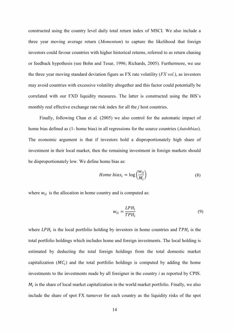
Finally, following Chan et al. (2005) we also control for the automatic impact of

home bias defined as (1- home bias) in all regressions for the source countries (Autohbias).

The economic argument is that if investors hold a disproportionately high share of

investment in their local market, then the remaining investment in foreign markets should

be disproportionately low. We define home bias as:

where 𝑤𝑖𝑖 is the allocation in home country and is computed as:

where 𝐿𝑃𝐻𝑖 is the local portfolio holding by investors in home countries and 𝑇𝑃𝐻𝑖 is the

total portfolio holdings which includes home and foreign investments. The local holding is

estimated by deducting the total foreign holdings from the total domestic market

capitalization (𝑀𝐶𝑖) and the total portfolio holdings is computed by adding the home

investments to the investments made by all foreigner in the country i as reported by CPIS.

𝑀𝑖 is the share of local market capitalization in the world market portfolio. Finally, we also

include the share of spot FX turnover for each country as the liquidity risks of the spot

𝐻𝑜𝑚𝑒 𝑏𝑖𝑎𝑠𝑖 = log (𝑤𝑖𝑖

𝑀𝑖) (8)

𝑤𝑖𝑖 =𝐿𝑃𝐻𝑖

𝑇𝑃𝐻𝑖 (9)

15

market could also deter investors. All the time varying control measures are either yearly

average or year-end values.

3. Empirical results

We begin the empirical analysis with the summary statistics on international portfolio

allocations, the three measures of market level FXD liquidity risks/trading costs, FX

volatility and control variables. We then presents the correlation matrix of all the factors

used in our regression analysis for the host countries, followed by the results of alternative

regression specifications.

3.1. Summary statistics

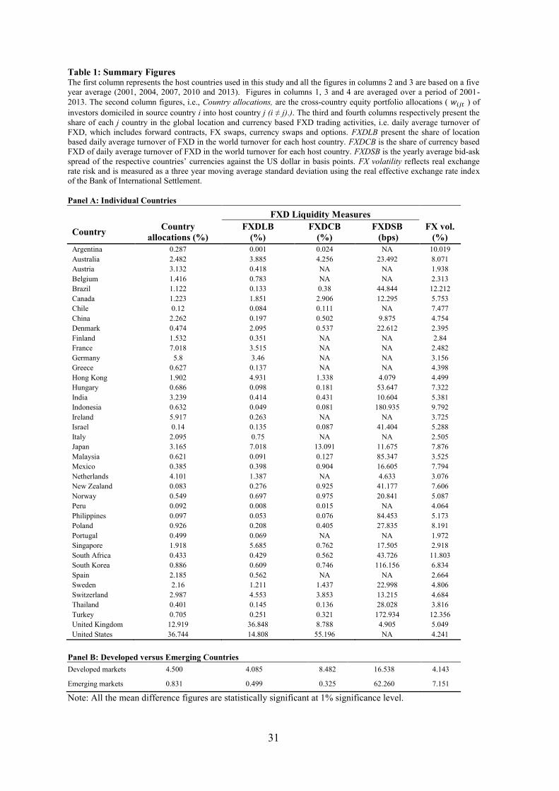
Table 1 shows summary figures for our five key variables. Panel A reports the figure

of individual countries and panel B the average figures of Panel A based on developed and

emerging market groups. Column two shows the average foreign equity allocations

received by the host countries from investors of all the source countries. In Panel A when

we sort the figures of column two from the highest allocations to the lowest it shows nine

of the top ten countries are occupied by developed markets. Supporting this in Panel B, the

average share of the developed markets in terms of receiving foreign portfolio allocations

is 4.5% compared to approximately 1% of those received by emerging markets. The

figures in Panel A (column two), show that the highest ranked country is the United States

followed by the United Kingdom, France, Ireland, Germany, Netherlands, India, Japan,

Austria and Switzerland. However, eight of the bottom ten ranked countries are emerging

markets (South Africa, Thailand, Mexico, Argentina, Israel, Chile, Philippines and Peru).28

28 Although theoretically these allocations should be driven by the size of each country’s equity market

capitalization in the world market portfolio, existing studies (see Chan et al., 2005) clearly note that foreign

investors generally prefer to invest more in developed markets relative to their theoretical prescription. In our

multivariate regression analysis we control for all possible factors driving the allocations, including the

theoretically prescribed ICAPM benchmark size.

16

We next focus on the relative rankings in the third column of Table 1 which show

the share of each country in the global OTC trading of FXD by location. Similar to figures

in column two, we see from Panel B (column three) that the share of the developed

markets’ currencies is 4.1% compared to 0.50% for the emerging markets. As expected

Panel A again shows that all the top ten positions are dominated by the currencies of

developed countries with the United Kingdom as the leader in the world trading of FXD

followed by the United States, Japan, Singapore, Hong Kong, Switzerland, Australia,

France, Germany and Denmark. Note the simple correlation coefficient between the

average figures of allocations and location based share of trading is 0.62, which provides

an indication that investors seem to prefer markets which have more developed and highly

liquid FXD markets.

Although, for the purpose of our study, the location based figures do capture the

heterogeneous transaction costs and liquidity risks of FXD markets, investors can

extensively trade third party currencies in major financial centres such as the United

Kingdom, the United States and Singapore. As such, as an additional measure of FXD

trading, we use the relative share of different currencies in the global trading and associate

each country with their respective currencies.29 Column 4 of Table 1 provides the five year

summary of 𝐹𝑋𝐷𝐶𝐵𝑗𝑡 and panel B shows, similar to the location based measure, that the

developed markets’ FX trading occupies a significantly higher share in the global trading

figures, an average of 8.5% compared to 0.32% for the emerging markets. All the top 10

rankings are taken by the developed countries’ currencies, with the United States being the

major currency of international reserve followed by Japan, the United Kingdom,30

Australia, Switzerland, Canada, Sweden, Hong Kong, Norway and New Zealand.

29 However, in the case of the Euro we are not able to distinguish the Euro countries as the relative

allocations are not provided by the BIS data. 30 In terms of currency the Euro occupies the second spot.

17

On comparing these countries with the allocations, we see that they are ranked

among the highest, as noted above. When we shift our attention to the countries whose

currencies are thinly traded with relatively underdeveloped FXD markets and hence are

lying in the bottom ten, they are all emerging markets (Turkey, Hungary, Chile, Thailand,

Malaysia, Israel, Indonesia, Argentina, Peru and Philippines). Correspondingly when we

compare these countries with the allocation figures of column 2, they all rank poorly as the

recipients of foreign portfolio allocations.

Column five of Table 1 reports (in basis points - bps) the one year bid-ask forward

rate to transact a unit US dollar. The average spread of the currencies of developed

markets is 16.5 bps compared to 62.2 bps for their emerging markets counterparts. Out of

the top ten countries with the lowest spread, seven are developed markets (Singapore,

Switzerland, Canada, Japan, United Kingdom, Netherlands and Hong Kong). Whereas, the

bottom ten with highest spread are all currencies of emerging markets (Indonesia, Turkey,

South Korea, Malaysia, Philippines, Hungary, Brazil, South Africa and Israel). This

supports the notion that it is expensive to transact emerging markets’ FXD.

Finally, column six (Panel A) reports the three moving average standard deviation

figures of the trade weighted real effective FX rate index of individual countries obtained

from the BIS.31 This figure provides an indication of the real FX risk faced by international

investors that is not captured by inflation differentials, i.e. in the scenario where PPP does

not hold. Panel B (column six) shows the average volatility of the FX rate for the

developed markets’ currencies is 4.14% compared to almost a twice greater figure of

7.15% for the currencies of emerging markets. The FX volatility figures are particularly

important for our study as they clearly show that compared to the developed countries,

currencies of most of the emerging markets are highly volatile and hence generate higher

FX risks.

31 We use this measure as a control in the regression analysis.

18

……………..Insert Table 1 about here…………….

Following the univariate analysis of Table 1, the figures suggest that investors’

allocations are relatively lower in countries/currencies which exhibit higher risks of FX

fluctuations (as indicated by the FX volatility figures). Furthermore, the summary analysis

of the first three variables (column 2-5) reported in Table 1, provides some reasonable

signal that foreign investors’ investments seem to be more associated with those markets

which provide liquid and cost-effective opportunities to hedge their FX risks

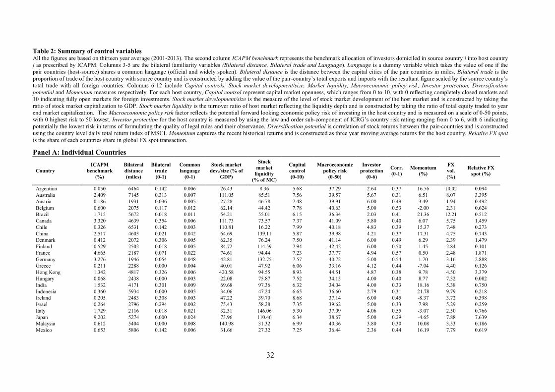
Table 2 reports all the host country-specific control variables used in our regressions.

As expected, compared to emerging markets, most of the developed markets rank higher in

terms of stock market size (ICAPM benchmark), have a greater trade share with the rest of

the world (bilateral trade), are legally more open (capital controls), have more developed

stock markets (size and liquidity), rank higher on macroeconomic policy risk and investor

protection (higher ranking denotes lower risk) and have higher cross-country correlation.


3.2. Correlation and regression results

In this section we begin our investigation with a pairwise correlation matrix followed

by regression estimations.

3.2.1. Correlation matrix

Table 3 shows (highlighted in bold) a statistically significant correlation coefficient

of FXDLB with country allocation of 0.40, which is the fourth highest figure for the

country allocation figures (column 2). Similarly, the correlation coefficient between

FXDCB and country allocation is 0.52 which is the third highest figure among all the

bilateral coefficients of country allocations. Note the figure of 0.52 for FXDCB is not

19

unexpected as the latter is a FX rate based turnover which better captures the heterogeneity

in FXD turnover, i.e. variations in the liquidity risks and transaction costs of FXD markets.

However, as we can see, both the FXD turnover factors, i.e. FXDLB and FXDCB have

fairly high levels of correlation between them, i.e. 0.62, indicating they both capture the

common variations in the FXD markets’ turnover. Finally, correlation figure between

country allocations and FXDSB is -0.36 indicating inverse co-movement between country

allocations and FXD transaction costs.

The statistically significant correlation coefficients of 0.35, 0.38 and -0.25 between

stock market liquidity and the three measures of FXD liquidity (i.e. FXDLB, FXDCB, and

FXDSB) respectively indicate that highly liquid equity markets also have highly liquid

FXD markets. Similarly, the statistically significant correlation coefficients between the

three FXD liquidity measures and FX volatility measures are -0.24, -0.22 and 0.37

respectively. This further suggests that the liquidity of FXD markets and levels of FX

volatility are inversely related, i.e. highly liquid FXD markets also seem to be associated

with a lower degree of FX risks. All other correlation coefficient figures are in line with

expectations, except for the macroeconomic policy risk and momentum.32


To summarize, the high and statistically significant coefficient figures of FXDLB,

FXDCB and FXDSB with country allocations signal that higher (lower) degree of FXD

turnover (costs) are associated with higher level of country allocations by foreign

investors. We further test the robustness of such association using the different regression

specifications.

32 Similar results are reported in literature (Gelos and Wei, 2005).

20

3.2.2. Regression results

As noted earlier, one of the advantages of our dataset is the panel set-up which

affords us greater statistical advantage in exploiting the wide cross-sectional (40 countries)

and temporal (2001-2013) variations.33 Given the fact that two of our variables are time

invariant (Distance and Language), we use the efficient GLS random effect model in all

our regressions but control for the country-specific and time fixed effects. Thus, our

econometric method exploits the country and time effects identification strategy. All the t-

statistics use the cluster-robust standard errors correcting for intra-clustering correlations

within individual panels.

We begin our investigation by estimating three regressions for the first measure

(𝐹𝑋𝐷𝐿𝐵𝑗𝑡) of the two turnover based variables, as shown in the specification below

(Equation 10):

The first regression (Equation 10) only includes the ICAPM benchmark and the most

widely explained factors of foreign portfolio allocations, i.e. the three bilateral familiarity

or information cost factors as controls. The second regression includes the benchmark,

bilateral familiarity and the two stock market development factors as control. Finally, the

third regression includes all other controls, such as capital control, macroeconomic policy

risk, investor protection, diversification potential, automatic impact of home bias,

momentum, FX volatility, Spot turnover, country fixed effects (country dummies) and

time fixed effects (year dummies). The results of the three regressions are reported in

Table 4.


33 Five years in case of BIS turnover based measures.

log(𝑤𝑖𝑗𝑡) = 𝛽. 𝐹𝑋𝐷𝐿𝐵𝑗𝑡 + 𝛾. 𝐶𝑜𝑛𝑡𝑟𝑜𝑙𝑠 + 𝑒𝑖𝑗𝑡 (10)

21

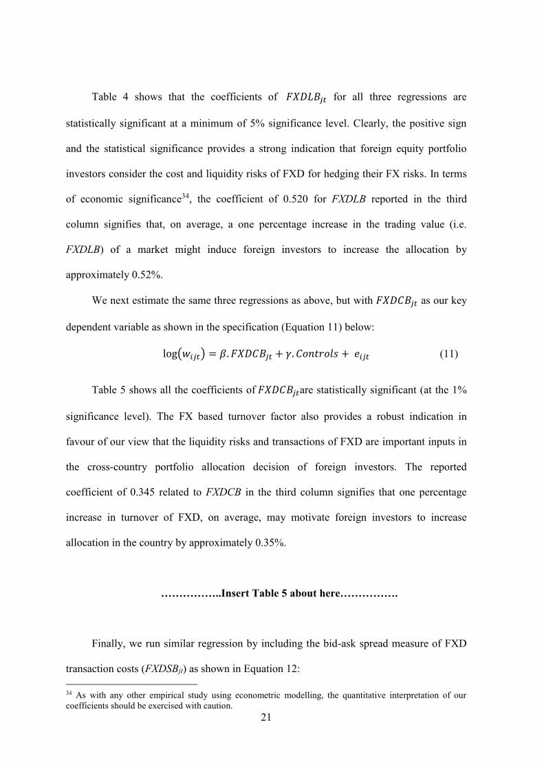
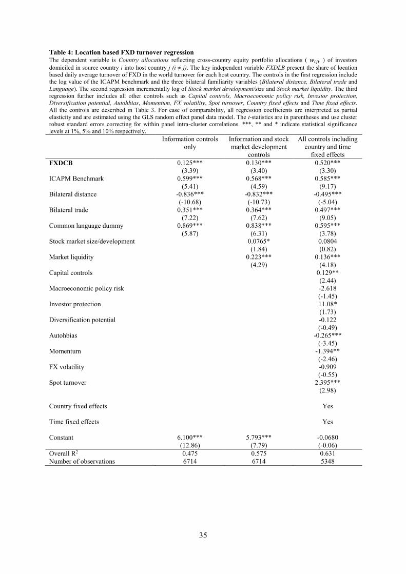
Table 4 shows that the coefficients of 𝐹𝑋𝐷𝐿𝐵𝑗𝑡 for all three regressions are

statistically significant at a minimum of 5% significance level. Clearly, the positive sign

and the statistical significance provides a strong indication that foreign equity portfolio

investors consider the cost and liquidity risks of FXD for hedging their FX risks. In terms

of economic significance34, the coefficient of 0.520 for FXDLB reported in the third

column signifies that, on average, a one percentage increase in the trading value (i.e.

FXDLB) of a market might induce foreign investors to increase the allocation by

approximately 0.52%.

We next estimate the same three regressions as above, but with 𝐹𝑋𝐷𝐶𝐵𝑗𝑡 as our key

dependent variable as shown in the specification (Equation 11) below:

Table 5 shows all the coefficients of 𝐹𝑋𝐷𝐶𝐵𝑗𝑡are statistically significant (at the 1%

significance level). The FX based turnover factor also provides a robust indication in

favour of our view that the liquidity risks and transactions of FXD are important inputs in

the cross-country portfolio allocation decision of foreign investors. The reported

coefficient of 0.345 related to FXDCB in the third column signifies that one percentage

increase in turnover of FXD, on average, may motivate foreign investors to increase

allocation in the country by approximately 0.35%.


Finally, we run similar regression by including the bid-ask spread measure of FXD

transaction costs (FXDSBjt) as shown in Equation 12:

34 As with any other empirical study using econometric modelling, the quantitative interpretation of our

coefficients should be exercised with caution.

log(𝑤𝑖𝑗𝑡) = 𝛽. 𝐹𝑋𝐷𝐶𝐵𝑗𝑡 + 𝛾. 𝐶𝑜𝑛𝑡𝑟𝑜𝑙𝑠 + 𝑒𝑖𝑗𝑡 (11)

22

The regression results reported in Table 6 show that the spread based measure of

transaction costs are all statistically significant at 5% significance level and bear the

expected signs.35 The sign implies that higher the spread, i.e. transaction costs; lower is the

allocation in the concerned currency/country.


In terms of the controls and as expected, based on existing literature (see Chan et al.,

2005), the most consistent of all are the bilateral familiarity/information cost factors

followed by the stock market development, particularly stock market liquidity. Note these

factors, along with the FXD liquidity measure and ICAPM benchmark, explain almost

54% of the total variations in portfolio allocations with only 8% additional fit being

observed by incorporating all other controls, including the country and time dummies.

Except the Autohbias, Capital control and Spot turnover, all other factors seem to be

sensitive to different specifications as they either become insignificant or change signs.

However, such inconsistencies related to all other factors are also reported in the existing

literature (see Chan et al, 2005; Gelos and Wei, 2005). In the following sections, we

conduct additional tests to ensure our results are robust to different theoretical and

econometric specifications.

3.2.3. Dealing with endogeneity

In all our above specifications we dealt with the issue of omitted variable bias,

including country and time effects. Errunza (2001) notes that the growing investment

35 The results in second column use data for 13-year period (2001-2013). However, the inclusion of Spot

turnover, which is only available for five year period (2001, 2004, 2007, 2010, and 2013) from BIS drops the

number of observations in the third column.

log(𝑤𝑖𝑗𝑡) = 𝛽. 𝐹𝑋𝐷𝑆𝐵𝑗𝑡 + 𝛾. 𝐶𝑜𝑛𝑡𝑟𝑜𝑙𝑠 + 𝑒𝑖𝑗𝑡 (12)

23

activities of foreign investors may demand reforms in the capital market, implying that

greater foreign investments can encourage the development of the FXD markets, leading to

greater availability of hedging possibilities. If this conjecture holds, then all our FXD

liquidity factors can suffer from endogeneity problems arising from reverse causality.

Following Gelos and Wei (2005) in Equation 13 below, we estimate the full specification

but using a predetermined, one period, lagged value of the three measures of FXD

liquidity, (𝐹𝑋𝐷𝑗,𝑡−1) i.e. 𝐹𝑋𝐷𝐿𝐵𝑗𝑡−1, 𝐹𝑋𝐷𝐶𝐵𝑗𝑡−1 and 𝐹𝑋𝐷𝑆𝐵𝑗𝑡−1:

Table 7 shows that all the three lagged factors are statistically significant. Note that

the sizes of the estimates do not substantially alter, even though the variables represent a

lagged rather than a level effect, along with the loss of one year’s observations. These

results provide strong support to our assertion that even after addressing the reverse

causality issue, FXD liquidity seems to significantly influence the cross-country portfolio

allocation decision of foreign investors.


3.2.4. Tradability in major financial centres

Table 1 shows that countries having major financial centres, principally the United

Kingdom and the United States, are the major recipients of foreign investment. These are

generally considered to be major financial centres where FXD are traded and hence, our

results could be driven by these major currencies. Further, the trades on these currencies

can also cover third country exposures, predominantly of smaller emerging markets,

through cross hedging. This could again question our results. We address this issue by re-

estimating the complete specifications of Equations 10, 11, and 12but by excluding some

log(𝑤𝑖𝑗𝑡) = 𝛽. 𝐹𝑋𝐷𝑗,𝑡−1 + 𝛾. 𝐶𝑜𝑛𝑡𝑟𝑜𝑙𝑠 + 𝑒𝑖𝑗𝑡 (13)

24

of the major financial trading centres, such as the United States, the United Kingdom,

Japan, Singapore, Hong Kong and Netherlands from our sample as source and host

countries.

Table 8 shows the coefficients of all the three FXD liquidity measures are still

statistically significant, although the size of the estimates now changes, which is not

unexpected as the estimation now uses different levels of information in the dataset.

However, we see that our key findings remain intact even when we take the major

financial centre countries out of the sample.


3.2.5. Float adjusted benchmark

Dahlquist et al. (2003) show that not all stocks in different countries are freely

available to foreign investors. This implies that, despite the theoretical ground, investors

may not hold the world market portfolio. If stocks are not freely floated, our results may be

biased with the usage of the total world market portfolio as the benchmark. We address

this by re-constructing the benchmark, using equation no. 3 (see section 2.1), based on the

proportion of freely available market capitalization of Dahlquist et al. (2003) and re-run

the complete specifications of Equations 10, 11 and 12. The results are reported in Table

8.36


36 As an alternative measure, we also use the S&P/IFCI market capitalization, which is the investable market

capitalization, to construct the benchmark. The results of the regression are qualitatively similar. However,

since this measure is only available for emerging markets, we do not report these results in our paper.

25

The statistically significant coefficients of all the three relevant factors further

support our view that even after controlling for the possibility of free float issue, foreign

investors prefer to invest in those countries which have highly liquid FXD markets to

hedge the FX risks of their international portfolio investments.

3.2.6. Alternative measure

It can be argued that the two FXD turnover measures are based on their relative share

in the global trading activities of FXD, but they might not capture trading activities relative

to the size of their financial markets in which the trading takes place. In order to address

the effect of relative size of the corresponding economies, we employ an additional scaling

method to the total turnover figures reported in the BIS’s 2013 TCBS statistics (Table 19),

which include the yearly figure of the average daily spot and FXD trading (in billion USD)

in the month of April. We scale the aggregate figure by each country’s equity market

capitalization (in billion USD) and use it as an additional proxy reflecting the

heterogeneous degree of liquidity risks and transaction costs of FXD markets relative to

the size of the financial market. We denote this factor as 𝐹𝑋𝐷_𝑡𝑜_𝑀𝐶𝐴𝑃𝑗𝑡 and estimate

the following regression in equation 14:

Table 9 shows the highly statistically significant estimate of 𝐹𝑋𝐷_𝑡𝑜_𝑀𝐶𝐴𝑃𝑗𝑡

(0.513), (at a 1% significance level), and this indicates that economies which have highly

liquid FXD markets relative to the size of their economy attract higher levels of foreign

portfolio investments.


log(𝑤𝑖𝑗𝑡) = 𝛽. 𝐹𝑋𝐷_𝑡𝑜_𝑀𝐶𝐴𝑃𝑗𝑡 + 𝛾. 𝐶𝑜𝑛𝑡𝑟𝑜𝑙𝑠 + 𝑒𝑖𝑗𝑡 (14)

26

4. Conclusion

The literature suggests that despite the benefits of international diversification

opportunities, portfolio investments are exposed to FX risks. In terms of modelling

expected returns and optimizing the global portfolio, prior studies note that investors who

hedge their FX risks using FXD improve their risk-return profile. However, foreign

investors’ hedging prospects are constrained by the varying degrees of liquidity risks and

transaction costs of FXD markets. In this study we investigate whether portfolio investors’

cross-country portfolio allocation decisions are influenced by the liquidity risks and

transaction costs of FXD. Using an extensive dataset with wide cross-sectional (developed

and emerging markets) and temporal (four years) variations, and employing robust

analytical techniques, we report the following key findings.

Our univariate analysis reports significant variations in liquidity levels of FXD

markets. Our results report that compared to their developed counterparts, developing

countries have smaller and relatively illiquid FXD markets. Such relatively undeveloped

FXD markets generate higher liquidity risks and transaction costs for effectively hedging

the FX risks of international portfolios. Similarly, our extensive and robust regression

correlation and regression results provide convincing evidence that foreign investors tend

to allocate more wealth to countries which have bigger and more liquid FXD markets

offering liquid and cost-effective prospects of hedging the FX risks of their international

portfolio investments. The overall results, which are robust to various alternative

specifications, imply that reforms aimed at developing the FXD markets could be a

potential policy measure for attracting higher levels of foreign equity portfolio

investments.

27

References

Baltagi, B.H. (2008). Econometric Analysis of Panel Data, New York: John Wiley and

Sons.

Banti, C., & Phylaktis, K. (2015). FX market liquidity, funding constraints and capital

flows. Journal of International Money and Finance, 56, 114-134.

Bartram, S.M., Brown, G.W., & Fehle, F.R. (2009). International evidence on financial

derivative usage. Financial Management, 38, 185-206.

Bekaert, G., Harvey, C.R., & Lundblad, C. (2007). Liquidity and expected returns: lessons

from emerging markets. The Review of Financial Studies, 20, 1783-1831.

Bekaert, G., & Hodrick, R. (2012). International Financial Management (2nd Ed), New

Jersey: Pearson Education.

Bodnar, G.M., Hayt, G.S., & Marston, R.C. (1996). Wharton survey of derivatives usage

by US non-financial firms. Financial Management, 25, 113-133.

Bohn, H., & Tesar, L.L. (1996). U.S. equity investment in foreign markets: Portfolio

rebalancing or return chasing? American Economic Review, 86, 77-81.

Campello, M., Lin C., Ma, Y., & Zou, H. (2011). The real and financial implications of

corporate hedging. Journal of Finance, 66, 1615 – 1647.

Cao, C., Ghysels, E., & Hatheway, F. (2011). Derivatives do affect mutual fund returns:

Evidence from the financial crisis of 1998. The Journal of Futures Market, 31, 629-658.

Carrieri, F., Errunza, V., & Majerbi, B. (2006). Does emerging market exchange rate affect

equity price? Journal of Financial and Quantitative Analysis, 41, 511-540.

Chan, K., Covrig, V., & Ng, L. (2005). What determines the domestic bias and foreign

bias? Evidence from mutual fund equity allocations worldwide. Journal of Finance, 60,

1495-1534.

Chong, L.L., Chang, X-J, & Tan, S-H (2014). Determinants of corporate foreign exchange

risk hedging, Managerial Finance, 40, 176-188.

Cooper, I., & Kaplanis, E. (1986). Costs to cross border investment and international

equity market equilibrium. In: Edwards, J., Franks, J., Mayer, C., Schaefer, S. (Eds.),

Recent Developments in Corporate Finance (pp. 209-240), New York: Cambridge

University Press.

Culp, C. L & Mackay, R. J. (1994). Regulating derivatives: The current system and

proposed changes. Regulation, 4, 38-51.

Dahlquist, M., Pinkowitz, L., Stulz, R.M., & Williamson, R. (2003). Corporate governance

and the home bias. Journal of Financial and Quantitative Analysis, 38, 87-110.

28

De Jong, F., & de Roon, F.A. (2005). Time-varying market integration and expected

returns in emerging markets. Journal of Financial Economics, 78, 583-613.

De Santis, G., & Gerard, B. (1998). How big is the premium for currency risk? Journal of

Financial Economics, 49, 375-412.

Duffie, D, Li, A., & Lubke, T. (2010). Policy perspective on OTC derivatives market

infrastructure. Federal Reserve Bank of New York Staff Reports, 424, 1-25.

Dumas, D., & Solnik, M. (1995). The world price of foreign exchange risk. Journal of

Finance, 50, 445-479.

Errunza, V. (2001). Foreign portfolio equity investments, financial liberalization, and

economic development. Review of International Economics, 9, 703-726.

Eun, C., & Resnick, B. (1988). Exchange rate uncertainty, forward contracts and

international portfolio selection. Journal of Finance, 43, 197-215.

Eun, C., & Resnick, B. (1994). International diversification of investment portfolios: US

and Japanese perspectives. Management Science, 40, 140-161.

Fidora, M., Fratzscher, M., & Thimann, C. (2007). Home bias in global bond and equity

markets: The role of real exchange rate volatility. Journal of International Money and

Finance, 26, 631-655.

Gelos, R.G., & Wei, S-J. (2005). Transparency and international portfolio holdings.

Journal of Finance, 60, 2987-3020.

Glen, J., & Jorion, P. (1993). Currency hedging for international portfolios. Journal of

Finance, 48, 1865-1886.

Goyenko, R. Y., Holden, C. W., & Trzcinka, C. A. (2009). Do liquidity measures measure

liquidity? Journal of Financial Economics, 92(2), 153-181

Henderson, C. (2002). Editorial: Hedging emerging market currency risk. Derivative Use,

Trading and Regulation, 8, 5-12.

Jorion, P. (1989). Asset allocation with hedged and unhedged foreign stocks and bonds.

Journal of Portfolio Management, 15, 49-54.

Jorion, P. (1993). Currency hedging of international portfolios. Journal of Finance, 68,

1865-1866.

La Porta, R., Lopez-De-Silanes, F., Shleifer, A., & Vishny, R.W. (1998). Law and finance.

Journal of Political Economy, 106, 1113-1155.

Levine, R. & Zervos, S. (1998a), Stock markets, banks, and economic growth. American

Economic Review, 88, 537-558.

Levine, R., & Zervos, S. (1998b). Capital control liberalization and stock market

development. World Development, 26, 1169-1183.

29

Madura, J., & Fox, R. (2011). International Financial Management. (2nd Ed). United

Kingdom: Cengage Learning EMEA.

Mihaljek, D., & Packer, F. (2010). Derivatives in emerging markets. BIS Quarterly

Review, December, 43-58.

Perold, A.F., & Schulman, E.C. (1988). The free lunch in currency hedging: Implications

for investment policy and performance standards. Financial Analyst Journal, 44, 45-50.

Portes, R., & Rey, H. (2005). The determinants of cross-border equity flows. Journal of

International Economics, 65, 269-296.

Richards, A. (2005). Big fish in small ponds: The trading behaviour and price impact of

foreign investors in Asian equity markets. Journal of Financial and Quantitative Analysis,

40, 1-27.

Subramanian, A., & Wei, S-J. (2007). The WTO promotes trade, strongly but unevenly.

Journal of International Economics, 72, 151-175.

Triennial Central Bank Survey (2013), Foreign exchange turnover in April 2013:

preliminary global results, Bank of International Settlement, September 2013.

Zhou, V. Y., & Wang, P. (2013). Managing foreign exchange risk with derivatives in UK

non-financial firms, International Review of Financial Analysis 29, 294-302

30

Appendix - Source and host countries

Source countries Host countries

Developed markets Developed markets Australia Australia

Austria Austria

Belgium Belgium

Canada Canada

Denmark Denmark

Finland Finland

France France

Germany Germany

Greece Greece

Hong Kong Hong Kong

Iceland Ireland

Ireland Italy

Israel Japan

Italy Netherlands

Japan New Zealand

Netherlands Norway

New Zealand Portugal

Norway Spain

Portugal Sweden

Spain Switzerland

Sweden United Kingdom

Switzerland United States

United Kingdom

United States Emerging markets

Argentina

Emerging markets Brazil

Argentina Chile

Bahrain China

Brazil Hungary

Bulgaria India

Chile Indonesia

Colombia Israel

Costa Rica Malaysia

Cyprus Mexico

Czech Republic Peru

Estonia Philippines

Egypt Poland

Hungary Singapore

India South Africa

Indonesia South Korea

Kazakhstan Thailand

Latvia Turkey

Lithuania

South Korea

Kuwait

Lebanon

Malaysia

Mauritius

Mexico

Pakistan

Panama

Philippines

Poland

Romania

Russia

Singapore

Slovenia

South Africa

Thailand

Turkey

Ukraine

Uruguay

Venezuela

31

Table 1: Summary Figures The first column represents the host countries used in this study and all the figures in columns 2 and 3 are based on a five

year average (2001, 2004, 2007, 2010 and 2013). Figures in columns 1, 3 and 4 are averaged over a period of 2001-

2013. The second column figures, i.e., Country allocations, are the cross-country equity portfolio allocations ( 𝑤𝑖𝑗𝑡 ) of

investors domiciled in source country i into host country j (i ≠ j).). The third and fourth columns respectively present the

share of each j country in the global location and currency based FXD trading activities, i.e. daily average turnover of

FXD, which includes forward contracts, FX swaps, currency swaps and options. FXDLB present the share of location

based daily average turnover of FXD in the world turnover for each host country. FXDCB is the share of currency based

FXD of daily average turnover of FXD in the world turnover for each host country. FXDSB is the yearly average bid-ask

spread of the respective countries’ currencies against the US dollar in basis points. FX volatility reflects real exchange

rate risk and is measured as a three year moving average standard deviation using the real effective exchange rate index

of the Bank of International Settlement.

Panel A: Individual Countries

FXD Liquidity Measures

Country Country

allocations (%)

FXDLB

(%)

FXDCB

(%)

FXDSB

(bps)

FX vol.

(%)

Argentina 0.287 0.001 0.024 NA 10.019

Australia 2.482 3.885 4.256 23.492 8.071

Austria 3.132 0.418 NA NA 1.938

Belgium 1.416 0.783 NA NA 2.313

Brazil 1.122 0.133 0.38 44.844 12.212

Canada 1.223 1.851 2.906 12.295 5.753

Chile 0.12 0.084 0.111 NA 7.477

China 2.262 0.197 0.502 9.875 4.754

Denmark 0.474 2.095 0.537 22.612 2.395

Finland 1.532 0.351 NA NA 2.84

France 7.018 3.515 NA NA 2.482

Germany 5.8 3.46 NA NA 3.156

Greece 0.627 0.137 NA NA 4.398

Hong Kong 1.902 4.931 1.338 4.079 4.499

Hungary 0.686 0.098 0.181 53.647 7.322

India 3.239 0.414 0.431 10.604 5.381

Indonesia 0.632 0.049 0.081 180.935 9.792

Ireland 5.917 0.263 NA NA 3.725

Israel 0.14 0.135 0.087 41.404 5.288

Italy 2.095 0.75 NA NA 2.505

Japan 3.165 7.018 13.091 11.675 7.876

Malaysia 0.621 0.091 0.127 85.347 3.525

Mexico 0.385 0.398 0.904 16.605 7.794

Netherlands 4.101 1.387 NA 4.633 3.076

New Zealand 0.083 0.276 0.925 41.177 7.606

Norway 0.549 0.697 0.975 20.841 5.087

Peru 0.092 0.008 0.015 NA 4.064

Philippines 0.097 0.053 0.076 84.453 5.173

Poland 0.926 0.208 0.405 27.835 8.191

Portugal 0.499 0.069 NA NA 1.972

Singapore 1.918 5.685 0.762 17.505 2.918

South Africa 0.433 0.429 0.562 43.726 11.803

South Korea 0.886 0.609 0.746 116.156 6.834

Spain 2.185 0.562 NA NA 2.664

Sweden 2.16 1.211 1.437 22.998 4.806

Switzerland 2.987 4.553 3.853 13.215 4.684

Thailand 0.401 0.145 0.136 28.028 3.816

Turkey 0.705 0.251 0.321 172.934 12.356

United Kingdom 12.919 36.848 8.788 4.905 5.049

United States 36.744 14.808 55.196 NA 4.241

Panel B: Developed versus Emerging Countries

Developed markets 4.500 4.085 8.482 16.538 4.143

Emerging markets 0.831 0.499 0.325 62.260 7.151

Note: All the mean difference figures are statistically significant at 1% significance level.

32

Table 2: Summary of control variables All the figures are based on thirteen year average (2001-2013). The second column ICAPM benchmark represents the benchmark allocation of investors domiciled in source country i into host country

j as prescribed by ICAPM. Columns 3-5 are the bilateral familiarity variables (Bilateral distance, Bilateral trade and Language). Language is a dummy variable which takes the value of one if the

pair countries (host-source) shares a common language (official and widely spoken). Bilateral distance is the distance between the capital cities of the pair countries in miles. Bilateral trade is the

proportion of trade of the host country with source country and is constructed by adding the value of the pair-country’s total exports and imports with the resultant figure scaled by the source country’s

total trade with all foreign countries. Columns 6-12 include Capital controls, Stock market development/size, Market liquidity, Macroeconomic policy risk, Investor protection, Diversification

potential and Momentum measures respectively. For each host country, Capital control represent capital market openness, which ranges from 0 to 10, with 0 reflecting completely closed markets and

10 indicating fully open markets for foreign investments. Stock market development/size is the measure of the level of stock market development of the host market and is constructed by taking the

ratio of stock market capitalization to GDP. Stock market liquidity is the turnover ratio of host market reflecting the liquidity depth and is constructed by taking the ratio of total equity traded to year

end market capitalization. The Macroeconomic policy risk factor reflects the potential forward looking economic policy risk of investing in the host country and is measured on a scale of 0-50 points,

with 0 highest risk to 50 lowest. Investor protection for the host country is measured by using the law and order sub-component of ICRG’s country risk rating ranging from 0 to 6, with 6 indicating

potentially the lowest risk in terms of formulating the quality of legal rules and their observance. Diversification potential is correlation of stock returns between the pair-countries and is constructed

using the country level daily total return index of MSCI. Momentum captures the recent historical returns and is constructed as three year moving average returns for the host country. Relative FX spot

is the share of each countries share in global FX spot transaction.

Panel A: Individual Countries

Country

ICAPM

benchmark

(%)

Bilateral

distance

(miles)

Bilateral

trade

(0-1)

Common

language

(0-1)

Stock market

dev./size (% of

GDP)

Stock

market

liquidity

(% of MC)

Capital

control

(0-10)

Macroeconomic

policy risk

(0-50)

Investor

protection

(0-6)

Corr.

(0-1)

Momentum

(%)

FX

vol.

(%)

Relative FX

spot (%)

Argentina 0.050 6464 0.142 0.006 26.43 8.36 5.68 37.29 2.64 0.37 16.56 10.02 0.094

Australia 2.409 7145 0.313 0.007 111.05 85.51 7.56 39.57 5.67 0.31 6.51 8.07 3.395

Austria 0.186 1931 0.036 0.005 27.28 46.78 7.48 39.91 6.00 0.49 3.49 1.94 0.492

Belgium 0.600 2075 0.117 0.012 62.14 44.42 7.78 40.63 5.00 0.53 -2.00 2.31 0.624

Brazil 1.715 5672 0.018 0.011 54.21 55.01 6.15 36.34 2.03 0.41 21.36 12.21 0.512

Canada 3.320 4639 0.354 0.006 111.73 73.57 7.37 41.09 5.80 0.40 6.07 5.75 1.459

Chile 0.326 6531 0.142 0.003 110.81 16.22 7.99 40.18 4.83 0.39 15.37 7.48 0.273

China 2.517 4603 0.021 0.042 64.69 139.11 5.87 39.98 4.21 0.37 17.31 4.75 0.743

Denmark 0.412 2072 0.306 0.005 62.35 76.24 7.50 41.14 6.00 0.49 6.29 2.39 1.479

Finland 0.529 2502 0.018 0.005 84.72 114.59 7.94 42.42 6.00 0.50 1.45 2.84 0.101

France 4.665 2187 0.071 0.022 74.61 94.44 7.23 37.77 4.94 0.57 0.50 2.48 1.871

Germany 3.276 1946 0.054 0.048 42.81 132.75 7.57 40.72 5.00 0.54 1.70 3.16 2.888

Greece 0.211 2288 0.000 0.004 40.01 47.92 6.06 33.16 4.12 0.44 -7.04 4.40 0.126

Hong Kong 1.342 4817 0.326 0.006 420.58 94.55 8.93 44.51 4.87 0.38 9.78 4.50 3.379

Hungary 0.068 2438 0.000 0.003 22.08 75.87 7.52 34.15 4.00 0.40 8.77 7.32 0.082

India 1.532 4171 0.301 0.009 69.68 97.36 6.32 34.04 4.00 0.33 18.16 5.38 0.750

Indonesia 0.360 5934 0.000 0.005 34.06 47.24 6.65 36.60 2.79 0.31 21.78 9.79 0.218

Ireland 0.205 2483 0.308 0.003 47.22 39.70 8.68 37.14 6.00 0.45 -8.37 3.72 0.398

Israel 0.264 2796 0.294 0.002 75.43 58.28 7.35 39.62 5.00 0.33 7.98 5.29 0.259

Italy 1.729 2116 0.018 0.021 32.31 146.06 5.30 37.09 4.06 0.55 -3.07 2.50 0.766

Japan 9.202 5274 0.000 0.024 73.96 110.46 6.34 38.67 5.00 0.29 -4.65 7.88 7.639

Malaysia 0.612 5404 0.000 0.008 140.98 31.32 6.99 40.36 3.80 0.30 10.08 3.53 0.186

Mexico 0.653 5806 0.142 0.006 31.66 27.32 7.25 36.44 2.36 0.44 16.19 7.79 0.619

33

Netherlands 1.289 2000 0.018 0.018 82.75 129.85 7.77 41.09 6.00 0.55 0.57 3.08 1.318

New Zealand 0.057 8616 0.306 0.001 40.60 40.95 7.77 37.38 5.65 0.19 2.89 7.61 0.141

Norway 0.490 2274 0.000 0.005 53.41 103.44 7.04 46.60 6.00 0.51 7.15 5.09 0.291

Peru 0.095 5836 0.159 0.002 50.75 6.53 7.31 37.91 3.16 0.35 25.21 4.06 0.060

Philippines 0.148 5436 0.302 0.002 60.68 18.79 6.00 37.18 2.35 0.18 9.19 5.17 0.070

Poland 0.248 2445 0.000 0.006 30.35 41.24 6.15 36.20 4.36 0.43 5.37 8.19 0.194

Portugal 0.187 2798 0.018 0.002 35.80 58.37 6.82 33.93 5.00 0.46 -1.94 1.97 0.115

Singapore 0.657 5295 0.301 0.010 165.82 66.75 8.79 44.81 5.14 0.43 7.24 2.92 6.165

South Africa 0.885 5721 0.319 0.003 184.84 51.75 6.77 35.19 2.36 0.43 14.69 11.80 0.285

South Korea 1.758 4988 0.306 0.011 76.19 206.62 6.15 41.45 4.84 0.34 14.03 6.83 1.215

Spain 1.562 2633 0.144 0.012 81.46 150.52 7.00 36.55 4.83 0.55 2.92 2.66 0.593

Sweden 1.062 2234 0.018 0.009 98.61 111.71 8.02 42.80 6.00 0.53 4.99 4.81 0.775

Switzerland 2.795 2014 0.126 0.008 200.89 93.29 7.71 44.05 5.06 0.53 0.50 4.68 4.644

Thailand 0.404 4828 0.302 0.006 70.92 88.67 6.32 37.87 2.85 0.32 12.71 3.82 0.181

Turkey 0.373 2462 0.000 0.005 31.33 149.28 6.44 32.51 4.10 0.39 26.72 12.36 0.195

United Kingdom 8.031 2255 0.306 0.023 120.12 131.18 8.38 36.83 5.58 0.53 2.92 5.05 30.222

United States 40.737 5254 0.302 0.068 117.28 197.50 7.24 37.33 5.09 0.36 1.17 4.24 28.155

Panel B: Developed versus Emerging Countries

Developed markets 3.832 3252 0.144 0.014 91.90 96.54 7.43 39.56 5.35 0.46 1.45 4.14 4.131

Emerging markets 0.704 4824 0.153 0.008 72.27 65.87 6.76 37.67 3.60 0.36 14.93 7.15 0.672

34

Table 3: Correlation matrix Country allocations are the cross-country equity portfolio allocations ( 𝑤𝑖𝑗𝑡 ) of investors domiciled in source country i into host country j (i ≠ j). FXDLB present the share of location based daily average turnover

of FXD in the world turnover for each host country. FXDCB is the share of currency based FXD of daily average turnover of FXD in the world turnover for each host country. FXDSB is the yearly average bid-ask

spread of the respective countries’ currencies against the US dollar. ICAPM benchmark is the benchmark allocation. Bilateral distance is the distance between the capital cities of the pair countries in miles.

Bilateral trade is the proportion of trade of the host country with source country and is constructed by adding the value of the pair-country’s total exports and imports with the resultant figure scaled by the source

country’s total trade with all foreign countries. Language is a dummy variable which takes the value of one if the pair countries (host-source) shares a common language (official and widely spoken). For each host

country, Capital control represent capital market openness, which ranges from 0 to 10, with 0 reflecting completely closed markets and 10 indicating fully open markets for foreign investments. Stock market

development/size is the measure of the level of stock market development of the host market and is constructed by taking the ratio of stock market capitalization to GDP. Stock market liquidity is the turnover ratio

of host market reflecting the liquidity depth and is constructed by taking the ratio of total equity traded to year end market capitalization. The Macroeconomic policy risk factor reflects the potential forward

looking economic policy risk of investing in the host country and is measured on a scale of 0-50 points, with 0 highest risk to 50 lowest. Investor protection for the host country is measured by using the law and

order sub-component of ICRG’s country risk rating ranging from 0 to 6, with 6 indicating potentially the lowest risk in terms of formulating the quality of legal rules and their observance. Diversification potential

is correlation of stock returns between the pair-countries and is constructed using the country level daily total return index of MSCI. Autohbias reflects the degree of home bias observed by investors of source

country reflecting the over allocations in their home markets relative to the suggested theory. Momentum captures the recent historical returns and is constructed as three year moving average returns for the host

country. FX volatility reflects real exchange rate risk and is measured as a three year moving average standard deviation using the real effective exchange rate index of the Bank of International Settlement. Relative

FX spot is the share of each countries share in global FX spot transaction.

(1) (2) (3) (4) (5) (6) (7) (8) (9) (10) (11) (12) (13) (14) (15) (16) (17)

Country allocations (1) 1

FXDLB (2) 0.40*** 1

FXDCD (3) 0.52*** 0.62*** 1

FXDSB (4) -0.36*** -0.14*** -0.18*** 1

ICAPM benchmark (5) 0.64** 0.5*** 0.67*** -0.27*** 1

Bilateral distance (6) -0.3*** -0.11*** 0.01 0.00 0.04* 1

Bilateral trade (7) 0.54*** 0.31*** 0.36*** -0.1*** 0.49*** -0.42*** 1

Language (8) 0.19*** 0.09*** -0.03 -0.06*** 0.01 0.04* 0.14*** 1

Capital control (9) 0.16*** 0.33*** 0.14*** 0.02 0.03 -0.07*** 0.01 0.09*** 1

Stock market dev./size (10) 0.32*** 0.26*** 0.17*** -0.25*** 0.55*** 0.06*** 0.15*** 0.17*** 0.35*** 1

Stock market liquidity (11) 0.27*** 0.35*** 0.38*** -0.25** 0.48*** -0.11*** 0.33*** -0.02 -0.01 0.16*** 1

Macroeconomic policy risk (12) 0.16*** -0.03 0.02 -0.33*** 0.20*** -0.07*** 0.07*** 0.04* 0.39*** 0.51*** 0.17*** 1

Investor protection (13) 0.22*** 0.3*** 0.34*** -0.19*** 0.27*** -0.19*** 0.11*** 0.06*** 0.43*** 0.27*** 0.42*** 0.49*** 1

Diversification potential (14) 0.32*** 0.17*** 0.03 -0.21*** 0.25*** -0.57*** 0.31*** -0.04* -0.02 0.20*** 0.21*** 0.15*** 0.15*** 1

Autohbias (15) -0.14*** -0.04* -0.04* -0.01 -0.02 -0.11*** -0.11*** -0.10*** -0.11*** -0.01 -0.01 -0.07*** -0.02 0.18*** 1

Momentum (16) -0.12*** -0.21*** -0.38*** 0.33*** -0.17*** 0.05** -0.06*** -0.04* 0.05** -0.07*** 0.13*** -0.06*** -0.32*** -0.06*** -0.08*** 1

FX volatility (17) -0.08*** -0.24*** -0.22*** 0.37*** -0.09*** 0.15*** -0.08*** -0.12*** -0.23*** -0.35*** -0.09*** -0.28*** -0.41*** -0.17*** 0.04* 0.09*** 1

***, ** and * indicate statistical significance levels at 1%, 5% and 10% respectively.

35

Table 4: Location based FXD turnover regression The dependent variable is Country allocations reflecting cross-country equity portfolio allocations ( 𝑤𝑖𝑗𝑡 ) of investors

domiciled in source country i into host country j (i ≠ j). The key independent variable FXDLB present the share of location

based daily average turnover of FXD in the world turnover for each host country. The controls in the first regression include

the log value of the ICAPM benchmark and the three bilateral familiarity variables (Bilateral distance, Bilateral trade and

Language). The second regression incrementally log of Stock market development/size and Stock market liquidity. The third

regression further includes all other controls such as Capital controls, Macroeconomic policy risk, Investor protection,

Diversification potential, Autohbias, Momentum, FX volatility, Spot turnover, Country fixed effects and Time fixed effects.

All the controls are described in Table 3. For ease of comparability, all regression coefficients are interpreted as partial

elasticity and are estimated using the GLS random effect panel data model. The t-statistics are in parentheses and use cluster

robust standard errors correcting for within panel intra-cluster correlations. ***, ** and * indicate statistical significance

levels at 1%, 5% and 10% respectively.

Information controls

only

Information and stock

market development

controls

All controls including

country and time

fixed effects

FXDCB 0.125*** 0.130*** 0.520***

(3.39) (3.40) (3.30)

ICAPM Benchmark 0.599*** 0.568*** 0.585***

(5.41) (4.59) (9.17)

Bilateral distance -0.836*** -0.832*** -0.495***

(-10.68) (-10.73) (-5.04)

Bilateral trade 0.351*** 0.364*** 0.497***

(7.22) (7.62) (9.05)

Common language dummy 0.869*** 0.838*** 0.595***

(5.87) (6.31) (3.78)

Stock market size/development 0.0765* 0.0804

(1.84) (0.82)

Market liquidity 0.223*** 0.136***

(4.29) (4.18)

Capital controls 0.129**

(2.44)

Macroeconomic policy risk -2.618

(-1.45)

Investor protection 11.08*

(1.73)

Diversification potential -0.122

(-0.49)

Autohbias -0.265***

(-3.45)

Momentum -1.394**

(-2.46)

FX volatility -0.909

(-0.55)

Spot turnover 2.395***

(2.98)

Country fixed effects Yes

Time fixed effects Yes

Constant 6.100*** 5.793*** -0.0680

(12.86) (7.79) (-0.06)

Overall R2 0.475 0.575 0.631

Number of observations 6714 6714 5348

36

Table 5: Currency distribution based FXD turnover regression The dependent variable is Country allocations reflecting cross-country equity portfolio allocations ( 𝑤𝑖𝑗𝑡 ) of investors

domiciled in source country i into host country j (i ≠ j). The key independent variable FXDCB present the share of currency

based daily average turnover of FXD in the world turnover for each host country. The controls in the first regression include

the log value of the ICAPM benchmark and the three bilateral familiarity variables (Bilateral distance, Bilateral trade and

Language). The second regression incrementally log of Stock market development/size and Stock market liquidity. The third

regression further includes all other controls such as Capital controls, Macroeconomic policy risk, Investor protection,

Diversification potential, Autohbias, Momentum, FX volatility, Spot turnover, Country fixed effects and Time fixed effects.

All the controls are described in Table 3. For ease of comparability, all regression coefficients are interpreted as partial

elasticity and are estimated using the GLS random effect panel data model. The t-statistics are in parentheses and use cluster

robust standard errors correcting for within panel intra-cluster correlations. ***, ** and * indicate statistical significance

levels at 1%, 5% and 10% respectively.


only


market development

controls


country and time

fixed effects

FXDCB 0.201*** 0.211*** 0.345***

(4.33) (4.86) (4.64)

ICAPM Benchmark 0.649*** 0.637*** 0.644***

(11.40) (8.30) (9.99)


(-9.80) (-9.93) (-5.44)

Bilateral trade 0.357*** 0.367*** 0.421***

(6.91) (7.15) (8.31)


(5.37) (5.67) (3.96)

Stock market size/ development 0.0500 0.0967

(1.61) (1.01)

Stock market liquidity 0.577*** 0.309***

(3.91) (3.46)


(2.40)

Macroeconomic policy risk 1.353

(1.14)

Investor protection -1.457

(-0.27)

Diversification potential 0.202

(0.85)

Autohbias -0.312***

(-3.48)

Momentum -0.338

(-0.81)

FX volatility 1.235

(1.27)


(5.27)


Year fixed effects Yes

Constant 5.947*** 6.023*** 0.170

(12.97) (7.66) (0.12)

Overall R2 0.527 0.628 0.683


37

Table 6: Bid-ask spread based regression The dependent variable is Country allocations reflecting cross-country equity portfolio allocations ( 𝑤𝑖𝑗𝑡 ) of investors

domiciled in source country i into host country j (i ≠ j). The key independent variable FXDSB is the yearly average bid-ask

spread of the respective countries’ currencies against the US dollar. The controls in the first regression include the log value

of the ICAPM benchmark and the three bilateral familiarity variables (Bilateral distance, Bilateral trade and Language).

The second regression incrementally log of Stock market development/size and Stock market liquidity. The third regression

further includes all other controls such as Capital controls, Macroeconomic policy risk, Investor protection, Diversification

potential, Autohbias, Momentum, FX volatility, Spot turnover, Country fixed effects and Time fixed effects. All the controls

are described in Table 3. For ease of comparability, all regression coefficients are interpreted as partial elasticity and are

estimated using the GLS random effect panel data model. The t-statistics are in parentheses and use cluster robust standard

errors correcting for within panel intra-cluster correlations. ***, ** and * indicate statistical significance levels at 1%, 5%

and 10% respectively.


only


market development

controls


country and time

fixed effects

FXDSB -0.111** -0.101** -0.326**

(-2.34) (-2.06) (-2.35)

ICAPM Benchmark 0.723*** 0.680*** 0.611***

(16.80) (13.90) (11.35)


(-13.39) (-13.17) (-4.52)

Bilateral trade 0.260*** 0.265*** 0.477***

(5.38) (5.41) (7.59)


(6.36) (6.37) (2.98)

Stock market size/development 0.0636 0.158*

(1.57) (1.70)

Stock market liquidity 0.920* 0.339***

(1.85) (3.49)


(2.41)


(-0.20)

Investor protection 8.850

(1.64)


(-0.26)

Autohbias -0.254***

(-3.17)

Momentum -0.675*

(-1.80)

FX volatility -1.850*

(-1.65)


(3.96)



Constant 5.797*** 4.952*** -1.165

(10.63) (8.60) (-0.89)

Overall R2 0.441 0.542 0.619


38

Table 7: Reverse causality The dependent variable in three regressions is the log value of equity portfolio country allocations ( 𝑤𝑖𝑗𝑡 ) of investors

domiciled in country i into country j (i ≠ j). The three key independent variables of interest are one period Lagged FXD

Turnover measures, i.e. FXDLBt-1, FXDCBt-1 and FXDSBt-1. The FXDLB, FXDCB, FXDSB and all the control variables are

described in Tables 3. For ease of comparability, all regression coefficients are interpreted as partial elasticity and are

estimated using the GLS random effect panel data model. The t-statistics are in parentheses and use cluster robust standard

errors correcting for within panel intra-cluster correlations. ***, ** and * indicate statistical significance levels at 1%,

5% and 10% respectively.

FXDLB FXDCB FXDSB

Lagged FXD liquidity 0.580*** 0.291*** -0.321***

(3.53) (3.20) (-2.56)

Benchmark 0.779*** 0.697*** 0.734***

(8.40) (10.66) (11.91)


(-5.22) (-5.60) (-5.28)

Bilateral trade 0.339*** 0.431*** 0.397***

(4.58) (6.29) (5.39)


(3.88) (3.63) (2.72)

Stock market size/development 0.0393 0.0204** 0.0885**

(1.38) (2.19) (1.98)

Stock market liquidity 0.0220*** 0.0569*** 0.0264***

(3.33) (3.66) (3.04)

Capital controls 0.0696** 0.177** 0.0501**

(2.19) (2.12) (2.31)

Macroeconomic policy risk 0.856 -2.934 -0.290

(0.65) (-1.57) (-0.37)

Investor protection -4.022 12.33 8.521

(-0.52) (1.49) (1.47)

Diversification potential 0.323 -0.182 -0.0867

(1.25) (-0.72) (-0.33)

Autohbias -0.273*** -0.237*** -0.254***

(-3.16) (-2.96) (-3.22)

Momentum -0.513 -1.477** -0.776*

(-0.87) (-2.03) (-1.71)

FX volatility -0.651 -2.553 -0.446

(-0.39) (-1.47) (-0.31)

Spot turnover 2.604*** 1.815*** 1.774***

(5.90) (2.67) (3.68)



Constant 0.580 0.800 -0.168

(0.40) (0.72) (-0.13)

Overall R2 0.684 0.633 0.625


39

Table 8: Regressions excluding major financial centres The dependent variable in all three regressions is the log value of equity portfolio country allocations ( 𝑤𝑖𝑗𝑡 ) of investors

domiciled in country i into country j. The three key independent variables of interest are FXD Liquidity measures, i.e.

FXDLB, FXDCB and FXDSB. The FXDLB, FXDCB, FXDSB and all the controls are described Table 3. Compared to the

full sample, the regression excludes major financial centres such as the United Kingdom, the United States, Japan,

Singapore, Hong Kong and the Netherlands from the sample. For ease of comparability, all regression coefficients are

interpreted as partial elasticity and are estimated using the GLS random effect panel data model. The t-statistics are in

parentheses and use cluster robust standard errors correcting for within panel intra-cluster correlations. ***, ** and *

indicate statistical significance levels at 1%, 5% and 10% respectively.

FXDLB FXDCB FXDSB

FXD Liquidity 0.144** 0.215*** -0.113***

(2.57) (3.05) (-3.80)

Benchmark 0.727*** 0.656*** 0.652***

(9.39) (7.41) (8.96)


(-4.88) (-4.84) (-4.01)

Bilateral trade 0.421*** 0.473*** 0.461***

(6.86) (7.06) (6.41)


(3.54) (3.81) (2.96)

Stock market size/development 0.127 0.0167** 0.103*

(1.35) (2.01) (1.68)

Stock market liquidity 0.077** 0.098** 0.0711**

(2.15) (2.01) (2.08)

Capital controls 0.0604** 0.162 0.0272

(2.14) (1.55) (1.57)

Macroeconomic policy risk 0.518 -2.813* -0.842

(0.41) (-1.69) (-0.70)


(-0.39) (1.48) (1.03)

Diversification potential 0.249 -0.0992 0.126

(0.88) (-0.35) (0.40)

Autohbias -0.308*** -0.295*** -0.243***

(-2.91) (-3.32) (-2.73)

Momentum -0.774** -1.659*** -0.753*

(-2.21) (-2.82) (-1.83)

FX volatility -1.909** -0.192 -2.326*

(-2.14) (-0.11) (-1.75)

Spot turnover 2.554*** 2.512*** 2.191***

(4.41) (3.40) (4.17)



Constant 1.913 0.578 -0.226

(1.17) (0.42) (-0.14)

Overall R2 0.680 0.628 0.609


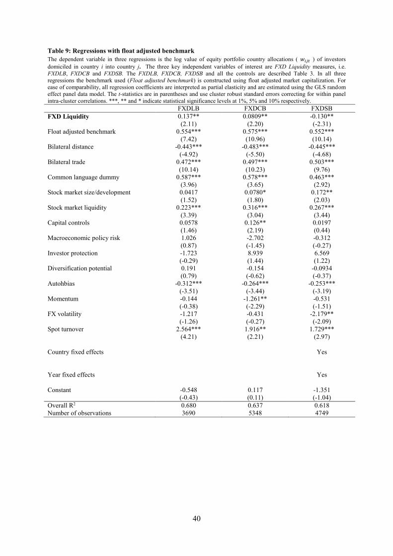
40

Table 9: Regressions with float adjusted benchmark

The dependent variable in three regressions is the log value of equity portfolio country allocations ( 𝑤𝑖𝑗𝑡 ) of investors

domiciled in country i into country j. The three key independent variables of interest are FXD Liquidity measures, i.e.

FXDLB, FXDCB and FXDSB. The FXDLB, FXDCB, FXDSB and all the controls are described Table 3. In all three

regressions the benchmark used (Float adjusted benchmark) is constructed using float adjusted market capitalization. For

ease of comparability, all regression coefficients are interpreted as partial elasticity and are estimated using the GLS random

effect panel data model. The t-statistics are in parentheses and use cluster robust standard errors correcting for within panel

intra-cluster correlations. ***, ** and * indicate statistical significance levels at 1%, 5% and 10% respectively.

FXDLB FXDCB FXDSB

FXD Liquidity 0.137** 0.0809** -0.130**

(2.11) (2.20) (-2.31)

Float adjusted benchmark 0.554*** 0.575*** 0.552***

(7.42) (10.96) (10.14)


(-4.92) (-5.50) (-4.68)

Bilateral trade 0.472*** 0.497*** 0.503***

(10.14) (10.23) (9.76)


(3.96) (3.65) (2.92)

Stock market size/development 0.0417 0.0780* 0.172**

(1.52) (1.80) (2.03)

Stock market liquidity 0.223*** 0.316*** 0.267***

(3.39) (3.04) (3.44)

Capital controls 0.0578 0.126** 0.0197

(1.46) (2.19) (0.44)

Macroeconomic policy risk 1.026 -2.702 -0.312

(0.87) (-1.45) (-0.27)


(-0.29) (1.44) (1.22)

Diversification potential 0.191 -0.154 -0.0934

(0.79) (-0.62) (-0.37)

Autohbias -0.312*** -0.264*** -0.253***

(-3.51) (-3.44) (-3.19)

Momentum -0.144 -1.261** -0.531

(-0.38) (-2.29) (-1.51)

FX volatility -1.217 -0.431 -2.179**

(-1.26) (-0.27) (-2.09)

Spot turnover 2.564*** 1.916** 1.729***

(4.21) (2.21) (2.97)



Constant -0.548 0.117 -1.351

(-0.43) (0.11) (-1.04)

Overall R2 0.680 0.637 0.618


41

Table 10: Regressions with an alternative proxy of FXD Turnover The dependent variable in the regression is the log value of equity portfolio country allocations ( 𝑤𝑖𝑗𝑡 ) of investors

domiciled in country i into country j. The key independent variable of interest is Alternative FXD Turnover Measure, which

is the total daily average of all FXD and spot transactions scaled by respective country’s equity market capitalization

(MCap). All the controls are described Table 3. For ease of comparability, all regression coefficients are interpreted as

partial elasticity and are estimated using the GLS random effect panel data model. The t-statistics are in parentheses and use

cluster robust standard errors correcting for within panel intra-cluster correlations. ***, ** and * indicate statistical

significance levels at 1%, 5% and 10% respectively.

Total FX Turnover to MCap

Alternative FXD Turnover Measure 0.3571**

(2.44)

ICAMP Benchmark 0.652***

(10.18)

Bilateral distance -0.527***

(-5.00)

Bilateral trade 0.473***

(8.05)

Common language dummy 0.581***

(3.72)

Stock market size/development 0.0514

(1.51)

Stock market liquidity 0.217**

(2.10)


(2.11)


(-1.54)

Investor protection 9.913

(1.61)


(-0.49)

Autohbias -0.269***

(-3.48)

Momentum -1.380**

(-2.57)

FX volatility -0.401

(-0.32)

Spot turnover 1.990**

(2.07)


Year Fixed effects Yes

Constant 0.319

(0.24)

Overall R2 0.632

Number of observations 5396

Market liquidity risks of foreign exchange derivatives and ...

Documents

Transcript of Market liquidity risks of foreign exchange derivatives and ...