Market Liquidity and Funding Liquiditymarkus/research/papers/...Market Liquidity and Funding...
38
Market Liquidity and Funding Liquidity Markus K. Brunnermeier Princeton University Lasse Heje Pedersen New York University We provide a model that links an asset’s market liquidity (i.e., the ease with which it is traded) and traders’ funding liquidity (i.e., the ease with which they can obtain funding). Traders provide market liquidity, and their ability to do so depends on their availability of funding. Conversely, traders’ funding, i.e., their capital and margin requirements, de- pends on the assets’ market liquidity. We show that, under certain conditions, margins are destabilizing and market liquidity and funding liquidity are mutually reinforcing, leading to liquidity spirals. The model explains the empirically documented features that market liquidity (i) can suddenly dry up, (ii) has commonality across securities, (iii) is related to volatility, (iv) is subject to “flight to quality,” and (v) co-moves with the market. The model provides new testable predictions, including that speculators’ capital is a driver of market liquidity and risk premiums. Trading requires capital. When a trader (e.g., a dealer, hedge fund, or investment bank) buys a security, he can use the security as collateral and borrow against it, but he cannot borrow the entire price. The difference between the security’s price and collateral value, denoted as the margin or haircut, must be financed with the trader’s own capital. Similarly, short-selling requires capital in the form of a margin; it does not free up capital. Therefore, the total margin on all positions cannot exceed a trader’s capital at any time. We are grateful for helpful comments from Tobias Adrian, Franklin Allen, Yakov Amihud, David Blair, Bernard Dumas, Denis Gromb, Charles Johns, Christian Julliard, John Kambhu, Markus Konz, Stefan Nagel, Michael Brennan, Martin Oehmke, Ketan Patel, Guillaume Plantin, Felipe Schwartzman, Hyun Shin, Matt Spiegel (the editor), Jeremy Stein, Dimitri Vayanos, Jiang Wang, Pierre-Olivier Weill, and from an anonymous referee and Filippos Papakonstantinou and Felipe Schwartzman for outstanding research assistantship. We also thank sem- inar participants at the New York Federal Reserve Bank, the New York Stock Exchange, Citigroup, Bank for International Settlement, University of Z¨ urich, INSEAD, Northwestern University, Stockholm Institute for Fi- nancial Research, Goldman Sachs, IMF, the World Bank, UCLA, LSE, Warwick University, Bank of England, University of Chicago, Texas A&M, University of Notre Dame, HEC, University of Maryland, University of Michigan, Virginia Tech, Ohio State University, University of Mannheim, ECB-Bundesbank, MIT, and confer- ence participants at the American Economic Association Meeting, FMRC conference in honor of Hans Stoll at Vanderbilt, NBER Market Microstructure Meetings, NBER Asset Pricing Meetings, NBER Risks of Financial Institutions conference, the Five Star conference, and American Finance Association Meeting. Brunnermeier acknowledges financial support from the Alfred P. Sloan Foundation. Send correspondence to Markus K. Brunnermeier, Princeton University, NBER and CEPR, Department of Economics, Bendheim Center for Finance, Princeton University, 26 Prospect Avenue, Princeton, NJ 08540-5296. E-mail: [email protected]. C The Author 2008. Published by Oxford University Press on behalf of The Society for Financial Studies. All rights reserved. For Permissions, please e-mail: [email protected]. doi:10.1093/rfs/hhn098 RFS Advance Access published December 10, 2008
Transcript of Market Liquidity and Funding Liquiditymarkus/research/papers/...Market Liquidity and Funding...
Market Liquidity and Funding Liquidity
Markus K. BrunnermeierPrinceton University
Lasse Heje PedersenNew York University
We provide a model that links an asset’s market liquidity (i.e., the ease with which it istraded) and traders’ funding liquidity (i.e., the ease with which they can obtain funding).Traders provide market liquidity, and their ability to do so depends on their availabilityof funding. Conversely, traders’ funding, i.e., their capital and margin requirements, de-pends on the assets’ market liquidity. We show that, under certain conditions, margins aredestabilizing and market liquidity and funding liquidity are mutually reinforcing, leadingto liquidity spirals. The model explains the empirically documented features that marketliquidity (i) can suddenly dry up, (ii) has commonality across securities, (iii) is related tovolatility, (iv) is subject to “flight to quality,” and (v) co-moves with the market. The modelprovides new testable predictions, including that speculators’ capital is a driver of marketliquidity and risk premiums.
Trading requires capital. When a trader (e.g., a dealer, hedge fund, or investmentbank) buys a security, he can use the security as collateral and borrow againstit, but he cannot borrow the entire price. The difference between the security’sprice and collateral value, denoted as the margin or haircut, must be financedwith the trader’s own capital. Similarly, short-selling requires capital in theform of a margin; it does not free up capital. Therefore, the total margin on allpositions cannot exceed a trader’s capital at any time.
We are grateful for helpful comments from Tobias Adrian, Franklin Allen, Yakov Amihud, David Blair, BernardDumas, Denis Gromb, Charles Johns, Christian Julliard, John Kambhu, Markus Konz, Stefan Nagel, MichaelBrennan, Martin Oehmke, Ketan Patel, Guillaume Plantin, Felipe Schwartzman, Hyun Shin, Matt Spiegel (theeditor), Jeremy Stein, Dimitri Vayanos, Jiang Wang, Pierre-Olivier Weill, and from an anonymous referee andFilippos Papakonstantinou and Felipe Schwartzman for outstanding research assistantship. We also thank sem-inar participants at the New York Federal Reserve Bank, the New York Stock Exchange, Citigroup, Bank forInternational Settlement, University of Zurich, INSEAD, Northwestern University, Stockholm Institute for Fi-nancial Research, Goldman Sachs, IMF, the World Bank, UCLA, LSE, Warwick University, Bank of England,University of Chicago, Texas A&M, University of Notre Dame, HEC, University of Maryland, University ofMichigan, Virginia Tech, Ohio State University, University of Mannheim, ECB-Bundesbank, MIT, and confer-ence participants at the American Economic Association Meeting, FMRC conference in honor of Hans Stoll atVanderbilt, NBER Market Microstructure Meetings, NBER Asset Pricing Meetings, NBER Risks of FinancialInstitutions conference, the Five Star conference, and American Finance Association Meeting. Brunnermeieracknowledges financial support from the Alfred P. Sloan Foundation. Send correspondence to Markus K.Brunnermeier, Princeton University, NBER and CEPR, Department of Economics, Bendheim Center forFinance, Princeton University, 26 Prospect Avenue, Princeton, NJ 08540-5296. E-mail: [email protected].
C© The Author 2008. Published by Oxford University Press on behalf of The Society for Financial Studies. Allrights reserved. For Permissions, please e-mail: [email protected]:10.1093/rfs/hhn098
RFS Advance Access published December 10, 2008
The Review of Financial Studies / v 00 n 0 2008
Our model shows that the funding of traders affects—and is affected by—market liquidity in a profound way. When funding liquidity is tight, tradersbecome reluctant to take on positions, especially “capital intensive” positions inhigh-margin securities. This lowers market liquidity, leading to higher volatil-ity. Further, under certain conditions, low future market liquidity increases therisk of financing a trade, thus increasing margins. Based on the links betweenfunding and market liquidity, we provide a unified explanation for the main em-pirical features of market liquidity. In particular, our model implies that marketliquidity (i) can suddenly dry up, (ii) has commonality across securities, (iii) isrelated to volatility, (iv) is subject to “flight to quality,” and (v) co-moves withthe market. The model has several new testable implications that link marginsand dealer funding to market liquidity: We predict that (i) speculators’ (mark-to-market) capital and volatility (as, e.g., measured by VIX) are state variablesaffecting market liquidity and risk premiums; (ii) a reduction in capital reducesmarket liquidity, especially if capital is already low (a nonlinear effect) and forhigh-margin securities; (iii) margins increase in illiquidity if the fundamentalvalue is difficult to determine; and (iv) speculators’ returns are negativelyskewed (even if they trade securities without skewness in the fundamentals).
Our model is similar in spirit to Grossman and Miller (1988) with the addedfeature that speculators face the real-world funding constraint discussed above.In our model, different customers have offsetting demand shocks, but arrive se-quentially to the market. This creates a temporary order imbalance. Speculatorssmooth price fluctuations, thus providing market liquidity. Speculators financetheir trades through collateralized borrowing from financiers who set the mar-gins to control their value-at-risk (VaR). Since financiers can reset margins ineach period, speculators face funding liquidity risk due to the risk of highermargins or losses on existing positions. We derive the competitive equilibriumof the model and explore its liquidity implications. We define market liquidityas the difference between the transaction price and the fundamental value, andfunding liquidity as speculators’ scarcity (or shadow cost) of capital.
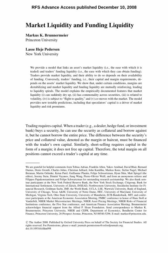
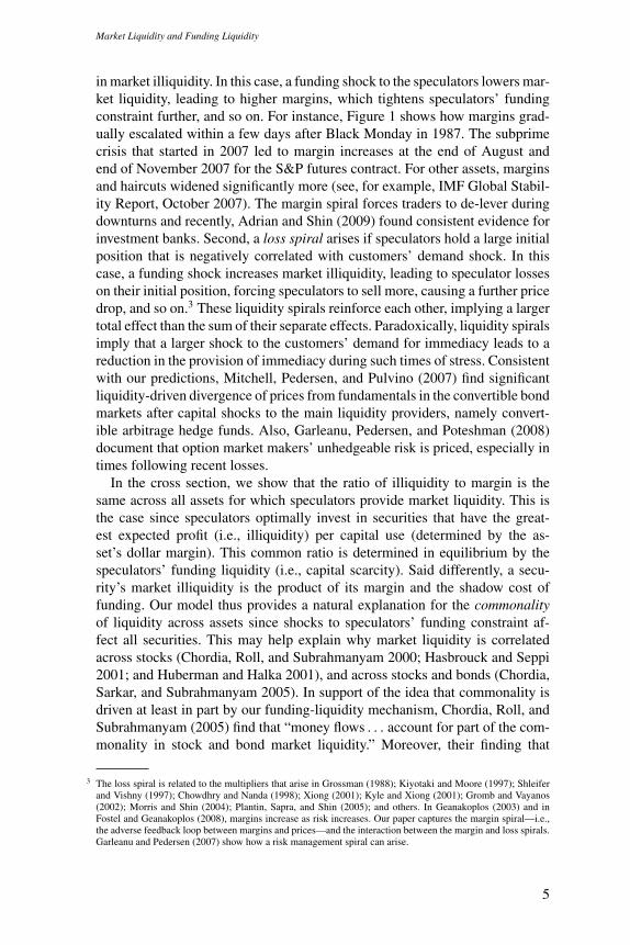
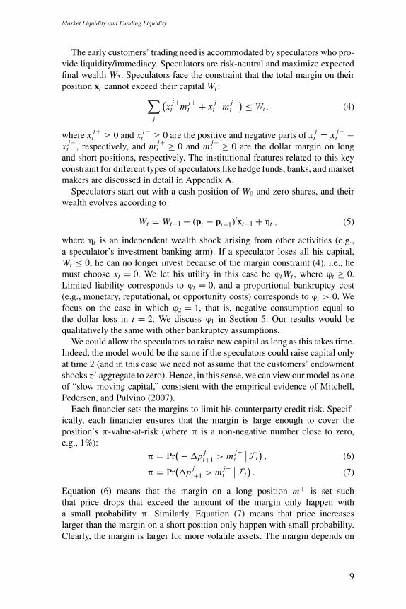
We first analyze the properties of margins, which determine the investors’capital requirement. We show that margins can increase in illiquidity whenmargin-setting financiers are unsure whether price changes are due to fun-damental news or to liquidity shocks, and volatility is time varying. Thishappens when a liquidity shock leads to price volatility, which raises the fi-nancier’s expectation about future volatility, and this leads to increased margins.Figure 1 shows that margins did increase empirically for S&P 500 futures dur-ing the liquidity crises of 1987, 1990, 1998, and 2007. More generally, theOctober 2007 IMF Global Stability Report documents a significant wideningof the margins across most asset classes during the summer of 2007. We denotemargins as “destabilizing” if they can increase in illiquidity, and note that anec-dotal evidence from prime brokers suggests that margins often behave in this
2
Market Liquidity and Funding Liquidity
0%
2%
4%
6%
8%
10%
12%
14%
Jan-82 Jan-84 Jan-86 Jan-88 Jan-90 Jan-92 Jan-94 Jan-96 Jan-98 Jan-00 Jan-02 Jan-04 Jan-06 Jan-08
Black Monday10/19/87
U.S. Iraq war
1989 mini-crash
LTCM
Asian crisis
Subprime crisis
Figure 1Margins for S&P 500 futuresThe figure shows margin requirements on S&P 500 futures for members of the Chicago Mercantile Exchangeas a fraction of the value of the underlying S&P 500 index multiplied by the size of the contract. (Initial ormaintenance margins are the same for members.) Each dot represents a change in the dollar margin.
way. Destabilizing margins force speculators to de-lever their positions in timesof crisis, leading to pro-cyclical market liquidity provision.1
In contrast, margins can theoretically decrease with illiquidity and thus canbe “stabilizing.” This happens when financiers know that prices diverge due totemporary market illiquidity and know that liquidity will be improved shortlyas complementary customers arrive. This is because a current price divergencefrom fundamentals provides a “cushion” against future adverse price moves,making the speculators’ position less risky in this case.
Turning to the implications for market liquidity, we first show that, as longas speculators’ capital is so abundant that there is no risk of hitting the fundingconstraint, market liquidity is naturally at its highest level and is insensitive tomarginal changes in capital and margins. However, when speculators hit theircapital constraints—or risk hitting their capital constraints over the life of atrade—then they reduce their positions and market liquidity declines. At thatpoint prices are more driven by funding liquidity considerations rather thanby movements in fundamentals, as was apparent during the quant hedge fundcrisis in August 2007, for instance.
When margins are destabilizing or speculators have large existing positions,there can be multiple equilibria and liquidity can be fragile. In one equilibrium,
1 The pro-cyclical nature of banks’ regulatory capital requirements and funding liquidity is another application ofour model, which we describe in Appendix A.2.
3
The Review of Financial Studies / v 00 n 0 2008
Funding problemsfor speculators
Reducedpositions
Highermargins
Losses on existing positions
Pricesmove away from
fundamentalsInitial losses
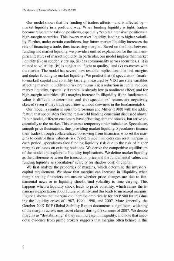
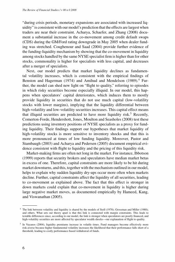
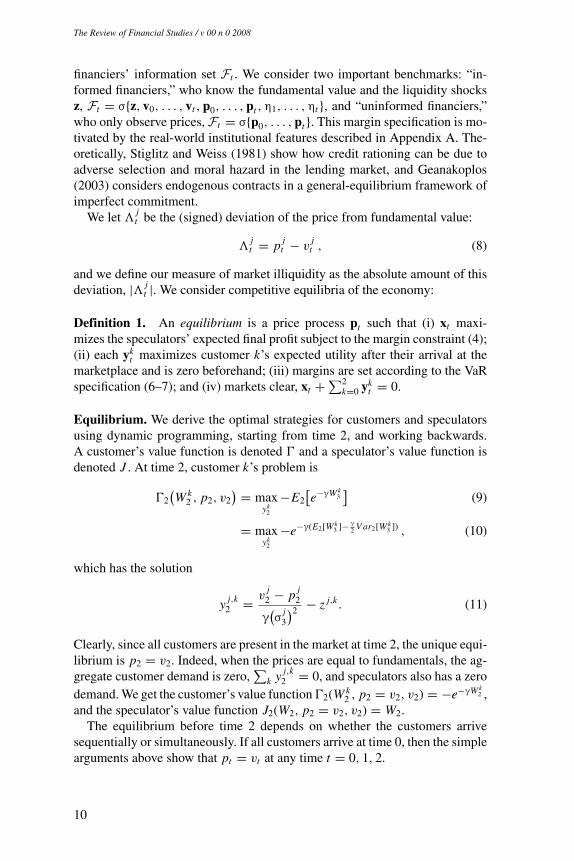
Figure 2Liquidity spiralsThe figure shows the loss spiral and the margin/haircut spiral.
markets are liquid, leading to favorable margin requirements for speculators,which in turn helps speculators make markets liquid. In another equilibrium,markets are illiquid, resulting in larger margin requirements (or speculatorlosses), thus restricting speculators from providing market liquidity. Impor-tantly, any equilibrium selection has the property that small speculator lossescan lead to a discontinuous drop of market liquidity. This “sudden dry-up” orfragility of market liquidity is due to the fact that with high levels of speculatorcapital, markets must be in a liquid equilibrium, and, if speculator capital isreduced enough, the market must eventually switch to a low-liquidity/high-margin equilibrium.2 The events following the Russian default and LTCMcollapse in 1998 are a vivid example of fragility of liquidity since a relativelysmall shock had a large impact. Compared to the total market capitalization ofthe U.S. stock and bond markets, the losses due to the Russian default wereminuscule but, as Figure 1 shows, caused a shiver in world financial markets.Similarly, the subprime losses in 2007–2008 were in the order of several hun-dred billion dollars, corresponding to only about 5% of overall stock marketcapitalization. However, since they were primarily borne by levered financialinstitutions with significant maturity mismatch, spiral effects amplified the cri-sis so, for example, the overall stock market losses amounted to more than 8trillion dollars as of this writing (see Brunnermeier 2009).
Further, when markets are illiquid, market liquidity is highly sensitive tofurther changes in funding conditions. This is due to two liquidity spirals, asillustrated in Figure 2. First, a margin spiral emerges if margins are increasing
2 Fragility can also be caused by asymmetric information on the amount of trading by portfolio insurance traders(Gennotte and Leland 1990), and by losses on existing positions (Chowdhry and Nanda 1998).
4
Market Liquidity and Funding Liquidity
in market illiquidity. In this case, a funding shock to the speculators lowers mar-ket liquidity, leading to higher margins, which tightens speculators’ fundingconstraint further, and so on. For instance, Figure 1 shows how margins grad-ually escalated within a few days after Black Monday in 1987. The subprimecrisis that started in 2007 led to margin increases at the end of August andend of November 2007 for the S&P futures contract. For other assets, marginsand haircuts widened significantly more (see, for example, IMF Global Stabil-ity Report, October 2007). The margin spiral forces traders to de-lever duringdownturns and recently, Adrian and Shin (2009) found consistent evidence forinvestment banks. Second, a loss spiral arises if speculators hold a large initialposition that is negatively correlated with customers’ demand shock. In thiscase, a funding shock increases market illiquidity, leading to speculator losseson their initial position, forcing speculators to sell more, causing a further pricedrop, and so on.3 These liquidity spirals reinforce each other, implying a largertotal effect than the sum of their separate effects. Paradoxically, liquidity spiralsimply that a larger shock to the customers’ demand for immediacy leads to areduction in the provision of immediacy during such times of stress. Consistentwith our predictions, Mitchell, Pedersen, and Pulvino (2007) find significantliquidity-driven divergence of prices from fundamentals in the convertible bondmarkets after capital shocks to the main liquidity providers, namely convert-ible arbitrage hedge funds. Also, Garleanu, Pedersen, and Poteshman (2008)document that option market makers’ unhedgeable risk is priced, especially intimes following recent losses.
In the cross section, we show that the ratio of illiquidity to margin is thesame across all assets for which speculators provide market liquidity. This isthe case since speculators optimally invest in securities that have the great-est expected profit (i.e., illiquidity) per capital use (determined by the as-set’s dollar margin). This common ratio is determined in equilibrium by thespeculators’ funding liquidity (i.e., capital scarcity). Said differently, a secu-rity’s market illiquidity is the product of its margin and the shadow cost offunding. Our model thus provides a natural explanation for the commonalityof liquidity across assets since shocks to speculators’ funding constraint af-fect all securities. This may help explain why market liquidity is correlatedacross stocks (Chordia, Roll, and Subrahmanyam 2000; Hasbrouck and Seppi2001; and Huberman and Halka 2001), and across stocks and bonds (Chordia,Sarkar, and Subrahmanyam 2005). In support of the idea that commonality isdriven at least in part by our funding-liquidity mechanism, Chordia, Roll, andSubrahmanyam (2005) find that “money flows . . . account for part of the com-monality in stock and bond market liquidity.” Moreover, their finding that
3 The loss spiral is related to the multipliers that arise in Grossman (1988); Kiyotaki and Moore (1997); Shleiferand Vishny (1997); Chowdhry and Nanda (1998); Xiong (2001); Kyle and Xiong (2001); Gromb and Vayanos(2002); Morris and Shin (2004); Plantin, Sapra, and Shin (2005); and others. In Geanakoplos (2003) and inFostel and Geanakoplos (2008), margins increase as risk increases. Our paper captures the margin spiral—i.e.,the adverse feedback loop between margins and prices—and the interaction between the margin and loss spirals.Garleanu and Pedersen (2007) show how a risk management spiral can arise.
5
The Review of Financial Studies / v 00 n 0 2008
“during crisis periods, monetary expansions are associated with increased liq-uidity” is consistent with our model’s prediction that the effects are largest whentraders are near their constraint. Acharya, Schaefer, and Zhang (2008) docu-ment a substantial increase in the co-movement among credit default swaps(CDS) during the GM/Ford rating downgrade in May 2005 when dealer fund-ing was stretched. Coughenour and Saad (2004) provide further evidence ofthe funding-liquidity mechanism by showing that the co-movement in liquidityamong stocks handled by the same NYSE specialist firm is higher than for otherstocks, commonality is higher for specialists with less capital, and decreasesafter a merger of specialists.
Next, our model predicts that market liquidity declines as fundamen-tal volatility increases, which is consistent with the empirical findings ofBenston and Hagerman (1974) and Amihud and Mendelson (1989).4 Fur-ther, the model can shed new light on “flight to quality,” referring to episodesin which risky securities become especially illiquid. In our model, this hap-pens when speculators’ capital deteriorates, which induces them to mostlyprovide liquidity in securities that do not use much capital (low-volatilitystocks with lower margins), implying that the liquidity differential betweenhigh-volatility and low-volatility securities increases. This capital effect meansthat illiquid securities are predicted to have more liquidity risk.5 Recently,Comerton-Forde, Hendershott, Jones, Moulton and Seasholes (2008) test thesepredictions using inventory positions of NYSE specialists as a proxy for fund-ing liquidity. Their findings support our hypotheses that market liquidity ofhigh-volatility stocks is more sensitive to inventory shocks and that this ismore pronounced at times of low funding liquidity. Moreover, Pastor andStambaugh (2003) and Acharya and Pedersen (2005) document empirical evi-dence consistent with flight to liquidity and the pricing of this liquidity risk.
Market-making firms are often net long in the market. For instance, Ibbotson(1999) reports that security brokers and speculators have median market betasin excess of one. Therefore, capital constraints are more likely to be hit duringmarket downturns, and this, together with the mechanism outlined in our model,helps to explain why sudden liquidity dry-ups occur more often when marketsdecline. Further, capital constraints affect the liquidity of all securities, leadingto co-movement as explained above. The fact that this effect is stronger indown markets could explain that co-movement in liquidity is higher duringlarge negative market moves, as documented empirically by Hameed, Kang,and Viswanathan (2005).
4 The link between volatility and liquidity is shared by the models of Stoll (1978); Grossman and Miller (1988);and others. What sets our theory apart is that this link is connected with margin constraints. This leads totestable differences since, according to our model, the link is stronger when speculators are poorly financed, andhigh-volatility securities are more affected by speculator wealth shocks—our explanation of flight to quality.
5 In Vayanos (2004), liquidity premiums increase in volatile times. Fund managers become effectively morerisk-averse because higher fundamental volatility increases the likelihood that their performance falls short of athreshold, leading to costly performance-based withdrawal of funds.
6
Market Liquidity and Funding Liquidity
Finally, the very risk that the funding constraint becomes binding limitsspeculators’ provision of market liquidity. Our analysis shows that speculators’optimal (funding) risk management policy is to maintain a “safety buffer.” Thisaffects initial prices, which increase in the covariance of future prices withfuture shadow costs of capital (i.e., with future funding illiquidity).
Our paper is related to several literatures.6 Traders rely both on (equity)investors and counterparties, and, while the limits to arbitrage literature fol-lowing Shleifer and Vishny (1997) focuses on the risk of investor redemptions,we focus on the risk that counterparty funding conditions may worsen. Othermodels with margin-constrained traders are Grossman and Vila (1992) andLiu and Longstaff (2004), which derive optimal strategies in a partial equilib-rium with a single security; Chowdhry and Nanda (1998) focus on fragilitydue to dealer losses; and Gromb and Vayanos (2002) derive a general equi-librium with one security (traded in two segmented markets) and study wel-fare and liquidity provision. We study the endogenous variation of marginconstraints, the resulting amplifying effects, and differences across high- andlow-margin securities in our setting with multiple securities. Stated simply,whereas the above-cited papers use a fixed or decreasing margin constraint,say, $5000 per contract, we study how market conditions lead to changes inthe margin requirement itself, e.g., an increase from $5000 to $15,000 perfutures contract as happened in October 1987, and the resulting feedbackeffects between margins and market conditions as speculators are forced tode-lever.
We proceed as follows. We describe the model (Section 1) and derive our fourmain new results: (i) margins increase with market illiquidity when financierscannot distinguish fundamental shocks from liquidity shocks and fundamentalshave time-varying volatility (Section 2); (ii) this makes margins destabilizing,leading to sudden liquidity dry-ups and margin spirals (Section 3); (iii) liquiditycrises simultaneously affect many securities, mostly risky high-margin securi-ties, resulting in commonality of liquidity and flight to quality (Section 4); and(iv) liquidity risk matters even before speculators hit their capital constraints(Section 5). Then we outline how our model’s new testable predictions may behelpful for a novel line of empirical work that links measures of speculators’funding conditions to measures of market liquidity (Section 6). Section 7 con-cludes. Finally, we describe the real-world funding constraints for the main liq-uidity providers, namely market makers, banks, and hedge funds (Appendix A),and provide proofs (Appendix B).
6 Market liquidity is the focus of market microstructure (Stoll 1978; Ho and Stoll 1981, 1983; Kyle 1985;Glosten and Milgrom 1985; Grossman and Miller 1988), and is related to the limits of arbitrage (DeLong et al.1990; Shleifer and Vishny 1997; Abreu and Brunnermeier 2002). Funding liquidity is examined in corporatefinance (Shleifer and Vishny 1992; Holmstrom and Tirole 1998, 2001) and banking (Bryant 1980; Diamondand Dybvig 1983; Allen and Gale 1998, 2004, 2005, 2007). Funding and collateral constraints are also studiedin macroeconomics (Aiyagari and Gertler 1999; Bernanke and Gertler 1989; Fisher 1933; Kiyotaki and Moore1997; Lustig and Chien 2005), and general equilibrium with incomplete markets (Geanakoplos 1997, 2003).Finally, recent papers consider illiquidity with constrained traders (Attari, Mello, and Ruckes 2005; Bernardoand Welch 2004; Brunnermeier and Pedersen 2005; Eisfeldt 2004; Morris and Shin 2004; Weill 2007).
7
The Review of Financial Studies / v 00 n 0 2008
1. Model
The economy has J risky assets, traded at times t = 0, 1, 2, 3. At time t = 3,each security j pays off v j , a random variable defined on a probability space(�,F ,P). There is no aggregate risk because the aggregate supply is zero andthe risk-free interest rate is normalized to zero, so the fundamental value of eachstock is its conditional expected value of the final payoff v
jt = Et [v j ]. Funda-
mental volatility has an autoregressive conditional heteroscedasticity (ARCH)structure. Specifically, v
jt evolves according to
vjt+1 = v
jt + �v
jt+1 = v
jt + σ
jt+1ε
jt+1 , (1)
where all εjt are i.i.d. across time and assets with a standard normal cumulative
distribution function � with zero mean and unit variance, and the volatility σjt
has dynamics
σjt+1 = σ j + θ j
∣∣�vjt
∣∣, (2)
where σ j , θ j ≥ 0. A positive θ j implies that shocks to fundamentals increasefuture volatility.
There are three groups of market participants: “customers” and “speculators”trade assets while “financiers” finance speculators’ positions. The group ofcustomers consists of three risk-averse agents. At time 0, customer k = 0, 1, 2has a cash holding of W k
0 bonds and zero shares, but finds out that he willexperience an endowment shock of zk = {z1,k, . . . , z J,k} shares at time t = 3,where z are random variables such that the aggregate endowment shock is zero,∑2
k=0 z j,k = 0.With probability (1 − a), all customers arrive at the market at time 0 and can
trade securities in each time period 0, 1, 2. Since their aggregate shock is zero,they can share risks and have no need for intermediation.
The basic liquidity problem arises because customers arrive sequentiallywith probability a, which gives rise to order imbalance. Specifically, in thiscase customer 0 arrives at time 0, customer 1 arrives at time 1, and customer2 arrives at time 2. Hence, at time 2 all customers are present, at time 1 onlycustomers 0 and 1 can trade, and at time 0 only customer 0 is in the market.
Before a customer arrives in the marketplace, his demand is ykt = 0, and
after he arrives he chooses his security position each period to maximize hisexponential utility function U (W k
3 ) = − exp{−γW k3 } over final wealth. Wealth
W kt , including the value of the anticipated endowment shock of zk shares,
evolves according to
W kt+1 = W k
t + (pt+1 − pt )′(yk
t + zk). (3)
The vector of total demand shock of customers who have arrived in the marketat time t is denoted by Zt :=∑t
k=0 zk .
8
Market Liquidity and Funding Liquidity
The early customers’ trading need is accommodated by speculators who pro-vide liquidity/immediacy. Speculators are risk-neutral and maximize expectedfinal wealth W3. Speculators face the constraint that the total margin on theirposition xt cannot exceed their capital Wt :∑
j
(x j+
t m j+t + x j−
t m j−t
) ≤ Wt , (4)
where x j+t ≥ 0 and x j−
t ≥ 0 are the positive and negative parts of x jt = x j+
t −x j−
t , respectively, and m j+t ≥ 0 and m j−
t ≥ 0 are the dollar margin on longand short positions, respectively. The institutional features related to this keyconstraint for different types of speculators like hedge funds, banks, and marketmakers are discussed in detail in Appendix A.
Speculators start out with a cash position of W0 and zero shares, and theirwealth evolves according to
Wt = Wt−1 + (pt − pt−1)′xt−1 + ηt , (5)
where ηt is an independent wealth shock arising from other activities (e.g.,a speculator’s investment banking arm). If a speculator loses all his capital,Wt ≤ 0, he can no longer invest because of the margin constraint (4), i.e., hemust choose xt = 0. We let his utility in this case be ϕt Wt , where ϕt ≥ 0.Limited liability corresponds to ϕt = 0, and a proportional bankruptcy cost(e.g., monetary, reputational, or opportunity costs) corresponds to ϕt > 0. Wefocus on the case in which ϕ2 = 1, that is, negative consumption equal tothe dollar loss in t = 2. We discuss ϕ1 in Section 5. Our results would bequalitatively the same with other bankruptcy assumptions.
We could allow the speculators to raise new capital as long as this takes time.Indeed, the model would be the same if the speculators could raise capital onlyat time 2 (and in this case we need not assume that the customers’ endowmentshocks z j aggregate to zero). Hence, in this sense, we can view our model as oneof “slow moving capital,” consistent with the empirical evidence of Mitchell,Pedersen, and Pulvino (2007).
Each financier sets the margins to limit his counterparty credit risk. Specif-ically, each financier ensures that the margin is large enough to cover theposition’s π-value-at-risk (where π is a non-negative number close to zero,e.g., 1%):
π = Pr(− �p j
t+1 > m j+t
∣∣Ft), (6)
π = Pr(�p j
t+1 > m j−t
∣∣Ft). (7)
Equation (6) means that the margin on a long position m+ is set suchthat price drops that exceed the amount of the margin only happen witha small probability π. Similarly, Equation (7) means that price increaseslarger than the margin on a short position only happen with small probability.Clearly, the margin is larger for more volatile assets. The margin depends on
9
The Review of Financial Studies / v 00 n 0 2008
financiers’ information set Ft . We consider two important benchmarks: “in-formed financiers,” who know the fundamental value and the liquidity shocksz, Ft = σ{z, v0, . . . , vt , p0, . . . , pt ,η1, . . . ,ηt }, and “uninformed financiers,”who only observe prices, Ft = σ{p0, . . . , pt }. This margin specification is mo-tivated by the real-world institutional features described in Appendix A. The-oretically, Stiglitz and Weiss (1981) show how credit rationing can be due toadverse selection and moral hazard in the lending market, and Geanakoplos(2003) considers endogenous contracts in a general-equilibrium framework ofimperfect commitment.
We let �jt be the (signed) deviation of the price from fundamental value:
�jt = p j
t − vjt , (8)
and we define our measure of market illiquidity as the absolute amount of thisdeviation, |� j
t |. We consider competitive equilibria of the economy:
Definition 1. An equilibrium is a price process pt such that (i) xt maxi-mizes the speculators’ expected final profit subject to the margin constraint (4);(ii) each yk
t maximizes customer k’s expected utility after their arrival at themarketplace and is zero beforehand; (iii) margins are set according to the VaRspecification (6–7); and (iv) markets clear, xt +∑2
k=0 ykt = 0.
Equilibrium. We derive the optimal strategies for customers and speculatorsusing dynamic programming, starting from time 2, and working backwards.A customer’s value function is denoted � and a speculator’s value function isdenoted J . At time 2, customer k’s problem is
�2(W k
2 , p2, v2) = max
yk2
−E2[e−γW k
3]
(9)
= maxyk
2
−e−γ(E2[W k3 ]− γ
2 V ar2[W k3 ]) , (10)
which has the solution
y j,k2 = v
j2 − p j
2
γ(σ
j3
)2 − z j,k . (11)
Clearly, since all customers are present in the market at time 2, the unique equi-librium is p2 = v2. Indeed, when the prices are equal to fundamentals, the ag-gregate customer demand is zero,
∑k y j,k
2 = 0, and speculators also has a zerodemand. We get the customer’s value function �2(W k
2 , p2 = v2, v2) = −e−γW k2 ,
and the speculator’s value function J2(W2, p2 = v2, v2) = W2.The equilibrium before time 2 depends on whether the customers arrive
sequentially or simultaneously. If all customers arrive at time 0, then the simplearguments above show that pt = vt at any time t = 0, 1, 2.
10
Market Liquidity and Funding Liquidity
We are interested in the case with sequential arrival of the customers suchthat the speculators’ liquidity provision is needed. At time 1, customers 0 and1 are present in the market, but customer 2 has not arrived yet. As above,customer k = 0, 1 has a demand and value function of
y j,k1 = v
j1 − p j
1
γ(σ
j2
)2 − z j,k (12)
�1(W k
1 , p1, v1) = − exp
⎧⎨⎩−γ
⎡⎣W k
1 +∑
j
(v
j1 − p j
1
)22γ(σ
j2
)2⎤⎦⎫⎬⎭ . (13)
At time 0, customer k = 0 arrives in the market and maximizesE0[�1(W k
1 , p1, v1)].At time t = 1, if the market is perfectly liquid so that p j
1 = vj1 for all j ,
then the speculators are indifferent among all possible positions x1. If somesecurities have p1 �= v1, then the risk-neutral speculators invest all his capitalsuch that his margin constraint binds. The speculators optimally trade onlyin securities with the highest expected profit per dollar used. The profit perdollar used is (v j
1 − p j1 )/m j+
1 on a long position and −(v j1 − p j
1 )/m j−1 on a
short position. A speculators’ shadow cost of capital, denoted φ1, is 1 plus themaximum profit per dollar used as long as he is not bankrupt:
φ1 = 1 + maxj
{max
(v
j1 − p j
1
m j+1
,−(v j
1 − p j1
)m j−
1
)}, (14)
where the margins for long and short positions are set by the financiers, asdescribed in the next section. If the speculators are bankrupt, W1 < 0, thenφ1 = ϕ1. Each speculator’s value function is therefore
J1(W1, p1, v1, p0, v0) = W1φ1 . (15)
At time t = 0, the speculator maximizes E0[W1φ1] subject to his capital con-straint (4).
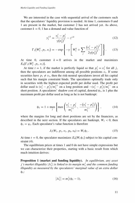
The equilibrium prices at times 1 and 0 do not have simple expressions butwe can characterize their properties, starting with a basic result from whichmuch intuition derives:
Proposition 1 (market and funding liquidity). In equilibrium, any assetj ’s market illiquidity |� j
1| is linked to its margin m j1 and the common funding
illiquidity as measured by the speculators’ marginal value of an extra dollarφ1: ∣∣� j
1
∣∣ = m j1(φ1 − 1), (16)
11
The Review of Financial Studies / v 00 n 0 2008
where m j1 = m j+
1 if the speculator is long and m j1 = m j−
1 otherwise. If thespeculators have a zero position for asset j , the equation is replaced by ≤.
We next go on to show the (de-)stabilizing properties of margins, and then wefurther characterize the equilibrium connection between market liquidity andspeculators’ funding situation, and the role played by liquidity risk at time 0.
2. Margin Setting and Liquidity (Time 1)
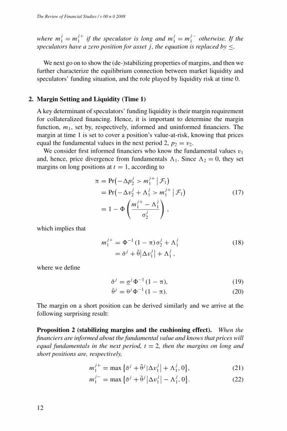
A key determinant of speculators’ funding liquidity is their margin requirementfor collateralized financing. Hence, it is important to determine the marginfunction, m1, set by, respectively, informed and uninformed financiers. Themargin at time 1 is set to cover a position’s value-at-risk, knowing that pricesequal the fundamental values in the next period 2, p2 = v2.
We consider first informed financiers who know the fundamental values v1
and, hence, price divergence from fundamentals �1. Since �2 = 0, they setmargins on long positions at t = 1, according to
π = Pr(−�p j
2 > m j+1
∣∣F1)
= Pr(−�v
j2 + �
j1 > m j+
1
∣∣F1)
(17)
= 1 − �
(m j+
1 − �j1
σj2
),
which implies that
m j+1 = �−1 (1 − π) σ
j2 + �
j1 (18)
= σ j + θ∣∣�v
j1
∣∣+ �j1 ,
where we define
σ j = σ j�−1 (1 − π), (19)
θ j = θ j�−1 (1 − π). (20)
The margin on a short position can be derived similarly and we arrive at thefollowing surprising result:
Proposition 2 (stabilizing margins and the cushioning effect). When thefinanciers are informed about the fundamental value and knows that prices willequal fundamentals in the next period, t = 2, then the margins on long andshort positions are, respectively,
m j+1 = max
{σ j + θ j |�v
j1
∣∣+ �j1, 0}, (21)
m j−1 = max
{σ j + θ j
∣∣�vj1
∣∣− �j1, 0}. (22)
12
Market Liquidity and Funding Liquidity
The more prices are below fundamentals �j1 < 0, the lower is the margin on
a long position m j+1 , and the more prices are above fundamentals �
j1 > 0, the
lower is the margin on a short position m j−1 . Hence, in this case illiquidity
reduces margins for speculators who buy low and sell high.
The margins are reduced by illiquidity because the speculators are expectedto profit when prices return to fundamentals at time 2, and this profit “cushions”the speculators from losses due to fundamental volatility. Thus, we denote themargins set by informed financiers at t = 1 as stabilizing margins.
Stabilizing margins are an interesting benchmark, and they are hard to escapein a theoretical model. However, real-world liquidity crises are often associatedwith increases in margins, not decreases. To capture this, we turn to the case ofa in which financiers are uninformed about the current fundamental so that hemust set his margin based on the observed prices p0 and p1. This is in generala complicated problem since the financiers need to filter out the probabilitythat customers arrive sequentially, and the values of z0 and z1. The expressionbecomes simple, however, if the financier’s prior probability of an asynchronousarrival of endowment shocks is small so that he finds it likely that p j
t = vjt ,
implying a common margin m j1 = m j+
1 = m j−1 for long and short positions in
the limit:
Proposition 3 (destabilizing margins). When the financiers are uninformedabout the fundamental value, then, as a → 0, the margins on long and shortpositions approach
m j1 = σ j + θ j
∣∣�p j1
∣∣ = σ j + θ j∣∣�v
j1 + ��
j1
∣∣ . (23)
Margins are increasing in price volatility and market illiquidity can increasemargins.
Intuitively, since liquidity risk tends to increase price volatility, and sinceuninformed financiers may interpret price volatility as fundamental volatility,this increases margins.7 Equation (23) corresponds closely to real-world marginsetting, which is primarily based on volatility estimates from past price move-ments. This introduces a procyclicality that amplifies funding shocks—a majorcriticism of the Basel II capital regulation. (See Appendix A.2 for how banks’capital requirements relate to our funding constraint.) Equation (23) shows thatilliquidity increases margins when the liquidity shock ��
j1 has the same sign
as the fundamental shock �vj1 (or is greater in magnitude), for example, when
bad news and selling pressure happen at the same time. On the other hand, mar-gins are reduced if the nonfundamental z-shock counterbalances a fundamental
7 In the analysis of time 0, we shall see that margins can also be destabilizing when price volatility signals futureliquidity risk (not necessarily fundamental risk).
13
The Review of Financial Studies / v 00 n 0 2008
move. We denote the phenomenon that margins can increase as illiquidity risesby destabilizing margins. As we will see next, the information available to thefinanciers (i.e., whether margins are stabilizing or destabilizing) has importantimplications for the equilibrium.
3. Fragility and Liquidity Spirals (Time 1)
We next show how speculators’ funding problems can lead to liquidity spiralsand fragility—the property that a small change in fundamentals can lead to alarge jump in illiquidity. We show that funding problems are especially esca-lating with uninformed financiers (i.e., destabilizing margins). For simplicity,we illustrate this with a single security J = 1.
3.1 FragilityTo set the stage for the main fragility proposition below, we make a few briefdefinitions. Liquidity is said to be fragile if the equilibrium price pt (ηt , vt )cannot be chosen to be continuous in the exogenous shocks, namely ηt and�vt . Fragility arises when the excess demand for shares xt +∑1
k=0 yk1 can
be non-monotonic in the price. While under “normal” circumstances, a highprice leads to a low total demand (i.e., excess demand is decreasing), bindingfunding constraints along with destabilizing margins (margin effect) or specu-lators’ losses (loss effect) can lead to an increasing demand curve. Further, it isnatural to focus on stable equilibria in which a small negative (positive) priceperturbation leads to excess demand (supply), which, intuitively, “pushes” theprice back up (down) to its equilibrium level.
Proposition 4 (fragility). There exist x, θ, a > 0 such that:(i) With informed financiers, the market is fragile at time 1 if speculators’position |x0| is larger than x and of the same sign as the demand shock Z1.(ii) With uninformed financiers the market is fragile as in (i) and additionallyif the ARCH parameter θ is larger than θ and the probability, a, of sequentialarrival of customers is smaller than a.
Numerical example. We illustrate how fragility arises due to destabilizingmargins or dealer losses by way of a numerical example. We consider themore interesting (and arguably more realistic) case in which the financiers areuninformed, and we choose parameters as follows.
The fundamental value has ARCH volatility parameters σ = 10 and θ =0.3, which implies clustering of volatility. The initial price is p0 = 130, theaggregate demand shock of the customers who have arrived at time 1 is Z1 =z0 + z1 = 30, and the customers’ risk aversion coefficient is γ = 0.05. Thespeculators have an initial position of x0 = 0 and a cash wealth of W1 =900. Finally, the financiers use a VaR with π = 1% and customers learn theirendowment shocks sequentially with probability a = 1%.
14
Market Liquidity and Funding Liquidity
−50 −40 −30 −20 −10 0 10 20 30 40 5090
100
110
120
130
140
150
160
170
x1
−50 −40 −30 −20 −10 0 10 20 30 40 50x1
p 1
90
100
110
120
130
140
150
160
170
p 1
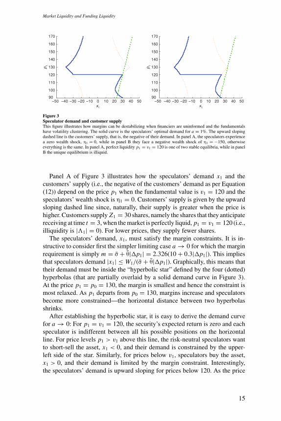
Figure 3Speculator demand and customer supplyThis figure illustrates how margins can be destabilizing when financiers are uninformed and the fundamentalshave volatility clustering. The solid curve is the speculators’ optimal demand for a = 1%. The upward slopingdashed line is the customers’ supply, that is, the negative of their demand. In panel A, the speculators experiencea zero wealth shock, η1 = 0, while in panel B they face a negative wealth shock of η1 = −150, otherwiseeverything is the same. In panel A, perfect liquidity p1 = v1 = 120 is one of two stable equilibria, while in panelB the unique equilibrium is illiquid.
Panel A of Figure 3 illustrates how the speculators’ demand x1 and thecustomers’ supply (i.e., the negative of the customers’ demand as per Equation(12)) depend on the price p1 when the fundamental value is v1 = 120 and thespeculators’ wealth shock is η1 = 0. Customers’ supply is given by the upwardsloping dashed line since, naturally, their supply is greater when the price ishigher. Customers supply Z1 = 30 shares, namely the shares that they anticipatereceiving at time t = 3, when the market is perfectly liquid, p1 = v1 = 120 (i.e.,illiquidity is |�1| = 0). For lower prices, they supply fewer shares.
The speculators’ demand, x1, must satisfy the margin constraints. It is in-structive to consider first the simpler limiting case a → 0 for which the marginrequirement is simply m = σ + θ|�p1| = 2.326(10 + 0.3|�p1|). This impliesthat speculators demand |x1| ≤ W1/(σ + θ|�p1|). Graphically, this means thattheir demand must be inside the “hyperbolic star” defined by the four (dotted)hyperbolas (that are partially overlaid by a solid demand curve in Figure 3).At the price p1 = p0 = 130, the margin is smallest and hence the constraint ismost relaxed. As p1 departs from p0 = 130, margins increase and speculatorsbecome more constrained—the horizontal distance between two hyperbolasshrinks.
After establishing the hyperbolic star, it is easy to derive the demand curvefor a → 0: For p1 = v1 = 120, the security’s expected return is zero and eachspeculator is indifferent between all his possible positions on the horizontalline. For price levels p1 > v1 above this line, the risk-neutral speculators wantto short-sell the asset, x1 < 0, and their demand is constrained by the upper-left side of the star. Similarly, for prices below v1, speculators buy the asset,x1 > 0, and their demand is limited by the margin constraint. Interestingly,the speculators’ demand is upward sloping for prices below 120. As the price
15
The Review of Financial Studies / v 00 n 0 2008
declines, the financiers’ estimate of fundamental volatility, and consequentlyof margins, increase.
We now generalize the analysis to the case where a > 0. The margin settingbecomes more complicated since uninformed financiers must filter out to whatextent the equilibrium price change is caused by a movement in fundamentals�v1 and/or an occurrence of a liquidity event with an order imbalance causedby the presence of customers 0 and 1, but not customer 2. Since customers0 and 1 want to sell (Z1 = 30), a price increase or modest price decline ismost likely due to a change in fundamentals, and hence the margin settingis similar to the case of a = 0. This is why speculators’ demand curve forprices above 100 almost perfectly overlays the relevant part of the hyperbolicstar in Figure 3. However, for a large price drop, say below 100, financiers assigna larger conditional probability that a liquidity event has occurred. Hence, theyare willing to set a lower margin (relative to the one implying the hyperbolicstar) because they expect the speculator to profit as the price rebounds in period2—hence, the cushioning effect discussed above reappears in the extreme here.This explains why the speculators’ demand curve is backward bending onlyin a limited price range and becomes downward sloping for p1 below roughly100.8
Panel A of Figure 3 shows that there are two stable equilibria: a perfectliquidity equilibrium with price p1 = v1 = 120 and an illiquid equilibriumwith a price of about 94 (and an uninteresting unstable equilibrium with p1 justbelow 120).
Panel B of Figure 3 shows the same plot as panel A, but with a negative wealthshock to speculators of η1 = −150 instead of η1 = 0. In this case, perfectliquidity with p1 = v1 is no longer an equilibrium since the speculators cannotfund a large enough position. The unique equilibrium is highly illiquid becauseof the speculators’ lower wealth and, importantly, because of endogenouslyhigher margins.
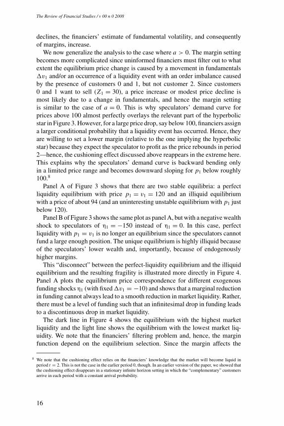
This “disconnect” between the perfect-liquidity equilibrium and the illiquidequilibrium and the resulting fragility is illustrated more directly in Figure 4.Panel A plots the equilibrium price correspondence for different exogenousfunding shocks η1 (with fixed �v1 = −10) and shows that a marginal reductionin funding cannot always lead to a smooth reduction in market liquidity. Rather,there must be a level of funding such that an infinitesimal drop in funding leadsto a discontinuous drop in market liquidity.
The dark line in Figure 4 shows the equilibrium with the highest marketliquidity and the light line shows the equilibrium with the lowest market liq-uidity. We note that the financiers’ filtering problem and, hence, the marginfunction depend on the equilibrium selection. Since the margin affects the
8 We note that the cushioning effect relies on the financiers’ knowledge that the market will become liquid inperiod t = 2. This is not the case in the earlier period 0, though. In an earlier version of the paper, we showed thatthe cushioning effect disappears in a stationary infinite horizon setting in which the “complementary” customersarrive in each period with a constant arrival probability.
16
Market Liquidity and Funding Liquidity
−100 −50 0 50 100 150 200 250 300 350 40090
100
110
120
130
140
150
η1
p 1
90
100
110
120
130
140
150
p 1
−30 −20 −10 0 10 20 30∆ v1
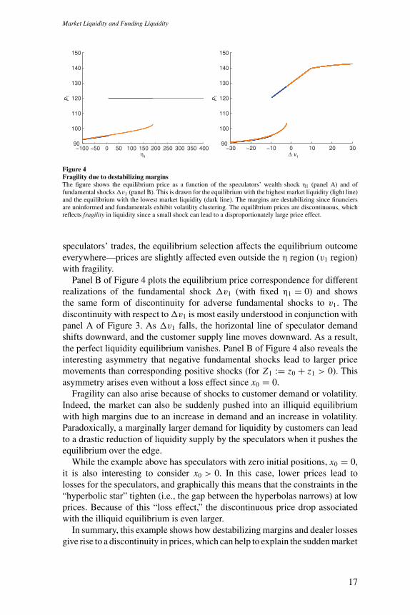
Figure 4Fragility due to destabilizing marginsThe figure shows the equilibrium price as a function of the speculators’ wealth shock η1 (panel A) and offundamental shocks �v1 (panel B). This is drawn for the equilibrium with the highest market liquidity (light line)and the equilibrium with the lowest market liquidity (dark line). The margins are destabilizing since financiersare uninformed and fundamentals exhibit volatility clustering. The equilibrium prices are discontinuous, whichreflects fragility in liquidity since a small shock can lead to a disproportionately large price effect.
speculators’ trades, the equilibrium selection affects the equilibrium outcomeeverywhere—prices are slightly affected even outside the η region (v1 region)with fragility.
Panel B of Figure 4 plots the equilibrium price correspondence for differentrealizations of the fundamental shock �v1 (with fixed η1 = 0) and showsthe same form of discontinuity for adverse fundamental shocks to v1. Thediscontinuity with respect to �v1 is most easily understood in conjunction withpanel A of Figure 3. As �v1 falls, the horizontal line of speculator demandshifts downward, and the customer supply line moves downward. As a result,the perfect liquidity equilibrium vanishes. Panel B of Figure 4 also reveals theinteresting asymmetry that negative fundamental shocks lead to larger pricemovements than corresponding positive shocks (for Z1 := z0 + z1 > 0). Thisasymmetry arises even without a loss effect since x0 = 0.
Fragility can also arise because of shocks to customer demand or volatility.Indeed, the market can also be suddenly pushed into an illiquid equilibriumwith high margins due to an increase in demand and an increase in volatility.Paradoxically, a marginally larger demand for liquidity by customers can leadto a drastic reduction of liquidity supply by the speculators when it pushes theequilibrium over the edge.
While the example above has speculators with zero initial positions, x0 = 0,it is also interesting to consider x0 > 0. In this case, lower prices lead tolosses for the speculators, and graphically this means that the constraints in the“hyperbolic star” tighten (i.e., the gap between the hyperbolas narrows) at lowprices. Because of this “loss effect,” the discontinuous price drop associatedwith the illiquid equilibrium is even larger.
In summary, this example shows how destabilizing margins and dealer lossesgive rise to a discontinuity in prices, which can help to explain the sudden market
17
The Review of Financial Studies / v 00 n 0 2008
liquidity dry-ups observed in many markets. For example, Russia’s default in1998 was in itself only a trivial wealth shock relative to global arbitrage capital.Nevertheless, it had a large effect on liquidity in global financial markets,consistent with our fragility result that a small wealth shock can push theequilibrium over the edge.
3.2 Liquidity SpiralsTo further emphasize the importance of speculators’ funding liquidity, we nowshow how it can make market liquidity highly sensitive to shocks. We identifytwo amplification mechanisms: a “margin spiral” due to increasing margins asspeculator financing worsens, and a “loss spiral” due to escalating speculatorlosses.
Figure 2 illustrates these “liquidity spirals.” A shock to speculator capital(η1 < 0) forces speculators to provide less market liquidity, which increasesthe price impact of the customer demand pressure. With uninformed financiersand ARCH effects, the resulting price swing increases financiers’ estimate ofthe fundamental volatility and, hence, increases the margin, thereby worseningspeculator funding problems even further, and so on, leading to a “marginspiral.” Similarly, increased market illiquidity can lead to losses on speculators’existing positions, worsening their funding problem and so on, leading to a “lossspiral.” Mathematically, the spirals can be expressed as follows:
Proposition 5. (i) If speculators’ capital constraint is slack, then the pricep1 is equal to v1 and insensitive to local changes in speculator wealth.(ii) (Liquidity spirals) In a stable illiquid equilibrium with selling pressurefrom customers, Z1, x1 > 0, the price sensitivity to speculator wealth shocksη1 is
∂p1
∂η1= 1
2γ(σ2)2 m+
1 + ∂m+1
∂p1x1 − x0
(24)
and with buying pressure from customers, Z1, x1 < 0,
∂p1
∂η1= −1
2γ(σ2)2 m−
1 + ∂m−1
∂p1x1 + x0
. (25)
A margin/haircut spiral arises if ∂m+1
∂p1< 0 or ∂m−
1∂p1
> 0, which happens withpositive probability if financiers are uninformed and a is small enough. A lossspiral arises if speculators’ previous position is in the opposite direction as thedemand pressure, x0 Z1 > 0.
This proposition is intuitive. Imagine first what happens if speculators facea wealth shock of $1, margins are constant, and speculators have no inventory
18
Market Liquidity and Funding Liquidity
x0 = 0. In this case, the speculator must reduce his position by 1/m1. Since theslope of each of the two customer demand curves is9 1/(γ(σ2)2), we get a totalprice effect of 1/( 2
γ(σ2)2 m1).The two additional terms in the denominator imply amplification or damp-
ening effects due to changes in the margin requirement and to profit/losseson the speculators’ existing positions. To see that, recall that for anyk > 0 and l with |l| < k, it holds that 1
k−l = 1k + l
k2 + l2
k3 + . . . ; so withk = 2
γ(σ2)2 m1 and l = − ∂m±1
∂p1x1 ± x0, each term in this infinite series corre-
sponds to one loop around the circle in Figure 2. The total effect of the changingmargin and speculators’ positions amplifies the effect if l > 0. Intuitively, withZ1 > 0, then customer selling pressure is pushing down the price, and ∂m+
1∂p1
< 0means that as prices go down, margins increase, making speculators’ fundingtighter and thus destabilizing the system. Similarly, when customers are buying,∂m−
1∂p1
> 0 implies that increasing prices leads to increased margins, making itharder for speculators to short-sell, thus destabilizing the system. The system isalso destabilized if speculators lose money on their previous position as pricesmove away from fundamentals.
Interestingly, the total effect of a margin spiral together with a loss spiral isgreater than the sum of their separate effects. This can be seen mathematicallyby using simple convexity arguments, and it can be seen intuitively from theflow diagram of Figure 2.
Note that spirals can also be “started” by shocks to liquidity demand Z1,fundamentals v1, or volatility. It is straightforward to compute the price sensi-tivity with respect to such shocks. They are just multiples of ∂p1
∂η1. For instance, a
fundamental shock affects the price both because of its direct effect on the finalpayoff and because of its effect on customers’ estimate of future volatility—andboth of these effects are amplified by the liquidity spirals.
Our analysis sheds some new light on the 1987 stock market crash, com-plementing the standard culprit, portfolio insurance trading. In the 1987 stockmarket crash, numerous market makers hit (or violated) their funding constraint:
“By the end of trading on October 19, [1987] thirteen [NYSEspecialist] units had no buying power,” —SEC (1988, chap. 4,p. 58)
While several of these firms managed to reduce their positions and continuetheir operations, others did not. For instance, Tompane was so illiquid that itwas taken over by Merrill Lynch Specialists and Beauchamp was taken over bySpear, Leeds & Kellogg (Beauchamp’s clearing broker). Also, market makersoutside the NYSE experienced funding troubles: the Amex market makersDamm Frank and Santangelo were taken over; at least 12 OTC market makersceased operations; and several trading firms went bankrupt.
9 See Equation (12).
19
The Review of Financial Studies / v 00 n 0 2008
These funding problems were due to (i) reductions in capital arising fromtrading losses and defaults on unsecured customer debt, (ii) an increased fund-ing need stemming from increased inventory, and (iii) increased margins. OneNew York City bank, for instance, increased margins/haircuts from 20% to 25%for certain borrowers, and another bank increased margins from 25% to 30%for all specialists (SEC, 1988, pp. 5–27 and 5–28). Other banks reduced thefunding period by making intraday margin calls, and at least two banks madeintraday margin calls based on assumed 15% and 25% losses, thus effectivelyincreasing the haircut by 15% and 25%. Also, some broker-dealers experienceda reduction in their line of credit and—as Figure 1 shows—margins at the fu-tures exchanges also drastically increased (SEC 1988 and Wigmore 1998).Similarly, during the ongoing liquidity and credit crunch, the margins and hair-cuts across most asset classes widened significantly starting in the summer of2007 (see IMF Global Stability Report, October 2007).
In summary, our results on fragility and liquidity spirals imply that dur-ing “bad” times, small changes in underlying funding conditions (or liquiditydemand) can lead to sharp reductions in liquidity. The 1987 crash exhibitedseveral of the predicted features, namely capital-constrained dealers, increasedmargins, and increased illiquidity.
4. Commonality and Flight to Quality (Time 1)
We now turn to the cross-sectional implications of illiquidity. Since speculatorsare risk-neutral, they optimally invest all their capital in securities that havethe greatest expected profit |� j | per capital use, i.e., per dollar margin m j , asexpressed in Equation (14). That equation also introduces the shadow cost ofcapital φ1 as the marginal value of an extra dollar. The speculators’ shadowcost of capital φ1 captures well the notion of funding liquidity: a high φ meansthat the available funding—from capital W1 and from collateralized financingwith margins m j
1—is low relative to the needed funding, which depends on theinvestment opportunities deriving from demand shocks z j .
The market liquidity of all assets depends on the speculators’ funding liq-uidity, especially for high-margin assets, and this has several interesting impli-cations:
Proposition 6. There exists c > 0 such that, for θ j < c for all j and eitherinformed financiers or uninformed with a < c, we have:
(i) Commonality of market liquidity. The market illiquidities |�| of anytwo securities, k and l, co-move,
Cov0(∣∣�k
1
∣∣, ∣∣�l1
∣∣) ≥ 0 , (26)
20
Market Liquidity and Funding Liquidity
and market illiquidity co-moves with funding illiquidity as measured byspeculators’ shadow cost of capital, φ1,
Cov0[∣∣�k
1
∣∣,φ1] ≥ 0 . (27)
(ii) Commonality of fragility. Jumps in market liquidity occur simultane-ously for all assets for which speculators are marginal investors.
(iii) Quality and liquidity. If asset l has lower fundamental volatility thanasset k, σl < σk , then l also has lower market illiquidity,∣∣�l
1
∣∣ ≤ ∣∣�k1
∣∣, (28)
if xk1 �= 0 or |Zk
1 | ≥ |Zl1|.
(iv) Flight to quality. The market liquidity differential between high- andlow-fundamental-volatility securities is bigger when speculator fundingis tight, that is, σl < σk implies that |�k
1| increases more with a negativewealth shock to the speculator,
∂∣∣�l
1
∣∣∂(−η1)
≤ ∂∣∣�k
1
∣∣∂(−η1)
, (29)
if xk1 �= 0 or |Zk
1 | ≥ |Zl1|. Hence, if xk
1 �= 0 or |Zk1 | ≥ |Zl
1| a.s., then
Cov0(∣∣�l
1
∣∣,φ1) ≤ Cov0
(∣∣�k1
∣∣,φ1). (30)
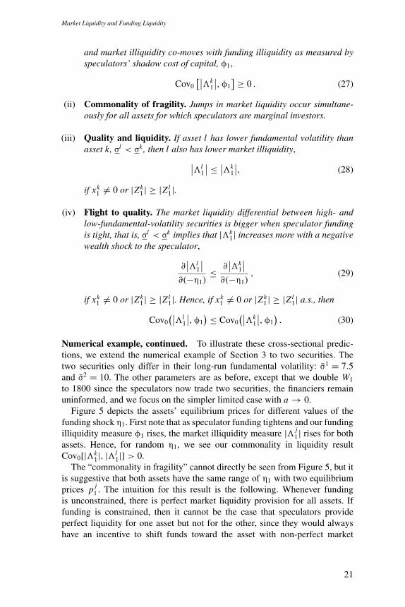
Numerical example, continued. To illustrate these cross-sectional predic-tions, we extend the numerical example of Section 3 to two securities. Thetwo securities only differ in their long-run fundamental volatility: σ1 = 7.5and σ2 = 10. The other parameters are as before, except that we double W1
to 1800 since the speculators now trade two securities, the financiers remainuninformed, and we focus on the simpler limited case with a → 0.
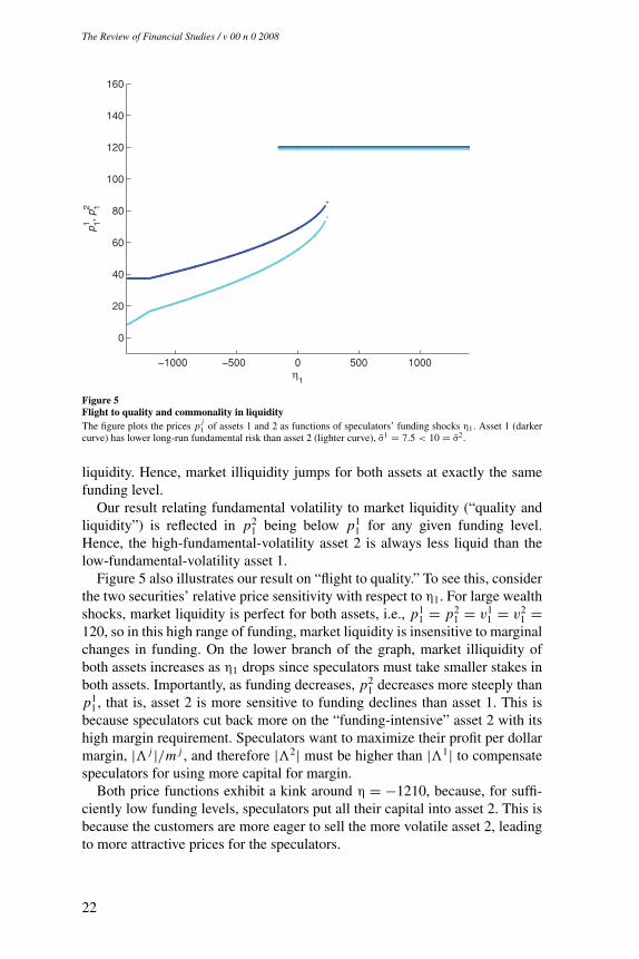
Figure 5 depicts the assets’ equilibrium prices for different values of thefunding shock η1. First note that as speculator funding tightens and our fundingilliquidity measure φ1 rises, the market illiquidity measure |� j
1| rises for bothassets. Hence, for random η1, we see our commonality in liquidity resultCov0[|�k
1|, |�l1|] > 0.
The “commonality in fragility” cannot directly be seen from Figure 5, but itis suggestive that both assets have the same range of η1 with two equilibriumprices p j
1 . The intuition for this result is the following. Whenever fundingis unconstrained, there is perfect market liquidity provision for all assets. Iffunding is constrained, then it cannot be the case that speculators provideperfect liquidity for one asset but not for the other, since they would alwayshave an incentive to shift funds toward the asset with non-perfect market
21
The Review of Financial Studies / v 00 n 0 2008
−1000 −500 0 500 1000
0
20
40
60
80
100
120
140
160
η1
p1 1, p2 1
Figure 5Flight to quality and commonality in liquidityThe figure plots the prices p j
1 of assets 1 and 2 as functions of speculators’ funding shocks η1. Asset 1 (darkercurve) has lower long-run fundamental risk than asset 2 (lighter curve), σ1 = 7.5 < 10 = σ2.
liquidity. Hence, market illiquidity jumps for both assets at exactly the samefunding level.
Our result relating fundamental volatility to market liquidity (“quality andliquidity”) is reflected in p2
1 being below p11 for any given funding level.
Hence, the high-fundamental-volatility asset 2 is always less liquid than thelow-fundamental-volatility asset 1.
Figure 5 also illustrates our result on “flight to quality.” To see this, considerthe two securities’ relative price sensitivity with respect to η1. For large wealthshocks, market liquidity is perfect for both assets, i.e., p1
1 = p21 = v1
1 = v21 =
120, so in this high range of funding, market liquidity is insensitive to marginalchanges in funding. On the lower branch of the graph, market illiquidity ofboth assets increases as η1 drops since speculators must take smaller stakes inboth assets. Importantly, as funding decreases, p2
1 decreases more steeply thanp1
1, that is, asset 2 is more sensitive to funding declines than asset 1. This isbecause speculators cut back more on the “funding-intensive” asset 2 with itshigh margin requirement. Speculators want to maximize their profit per dollarmargin, |� j |/m j , and therefore |�2| must be higher than |�1| to compensatespeculators for using more capital for margin.
Both price functions exhibit a kink around η = −1210, because, for suffi-ciently low funding levels, speculators put all their capital into asset 2. This isbecause the customers are more eager to sell the more volatile asset 2, leadingto more attractive prices for the speculators.
22
Market Liquidity and Funding Liquidity
5. Liquidity Risk (Time 0)
We now turn attention to the initial time period, t = 0, and demonstrate that(i) funding liquidity risk matters even before margin requirements actuallybind; (ii) the pricing kernel depends on future funding liquidity, φt+1; (iii) theconditional distribution of prices p1 is skewed due to the funding constraint(inducing fat tails ex ante); and (iv) margins m0 and illiquidity �0 can bepositively related due to liquidity risk even if financiers are informed.
The speculators’ trading activity at time 0 naturally depends on their expec-tations about the next period and, in particular, the time 1 illiquidity describedin detail above. Further, speculators risk having negative wealth W1 at time 1, inwhich case they have utility ϕt Wt . If speculators have no dis-utility associatedwith negative wealth levels (ϕt = 0), then they go to their limit already at time0 and the analysis is similar to time 1.
We focus on the more realistic case in which the speculators have dis-utilityin connection with W1 < 0 and, therefore, choose not to trade to their constraintat time t = 0 when their wealth is large enough. To understand this, note thatwhile most firms legally have limited liability, the capital Wt in our modelrefers to pledgable capital allocated to trading. For instance, Lehman Brothers’2001 Annual Report (p. 46) states:
“The following must be funded with cash capital: Secured funding ‘haircuts,’to reflect the estimated value of cash that would be advanced to the Companyby counterparties against available inventory, Fixed assets and goodwill, [and]Operational cash . . .”
Hence, if Lehman suffers a large loss on its pledgable capital such thatWt < 0, then it incurs monetary costs that must be covered with its unpledgablecapital like operational cash (which could also hurt Lehman’s other businesses).In addition, the firm incurs non-monetary cost, like loss in reputation andin goodwill, that reduces its ability to exploit future profitable investmentopportunities. To capture these effects, we let a speculator’s utility be φ1W1,where φ1 is given by the right-hand side of Equation (14) both for positiveand negative values of W1. With this assumption, equilibrium prices at timet = 0 are such that the speculators do not trade to their constraint at time t = 0when their wealth is large enough. In fact, this is the weakest assumption thatcurbs the speculators’ risk taking since it makes their objective function linear.Higher “bankruptcy costs” would lead to more cautious trading at time 0 andqualitatively similar results.10
10 We note that risk aversion also limits speculators’ trading in the real world. Our model based on marginconstraints differs from one driven purely by risk aversion in several ways. For example, an adverse shockthat lowers speculator wealth at t = 1 creates a profitable investment opportunity that one might think partiallyoffsets the loss—a natural “dynamic hedge.” Because of this dynamic hedge, in a model driven by risk-aversion,speculators (with a relative-risk-aversion coefficient larger than one) increase their t = 0 hedging demand, whichin turn, lowers illiquidity in t = 0. However, exactly the opposite occurs in a setting with capital constraints.Capital constraints prevent speculators from taking advantage of investment opportunities in t = 1 so they cannotexploit this “dynamic hedge.” Hence, speculators are reluctant to trade away the illiquidity at t = 0.
23
The Review of Financial Studies / v 00 n 0 2008
If the speculator is not constrained at time t = 0, then the first-order conditionfor his position in security j is E0[φ1(p j
1 − p j0 )] = 0. (We leave the case of
a constrained time-0 speculator for Appendix B.) Consequently, the fundingliquidity, φ1, determines the pricing kernel φ1/E0[φ1] for the cross section ofsecurities:
p j0 = E0
[φ1 p j
1
]E0[φ1]
= E0[
p j1
]+ Cov0[φ1, p j
1
]E0[φ1]
. (31)
Equation (31) shows that the price at time 0 is the expected time-1 price, whichalready depends on the liquidity shortage at time 1, further adjusted for liquidityrisk in the form of a covariance term. The liquidity risk term is intuitive: Thetime-0 price is lower if the covariance is negative, that is, if the security has alow payoff during future funding liquidity crises when φ1 is high.
An illustration of the importance of funding-liquidity management is the“LTCM crisis.” The hedge fund Long Term Capital Management (LTCM) hadbeen aware of funding liquidity risk. Indeed, they estimated that in times ofsevere stress, haircuts on AAA-rated commercial mortgages would increasefrom 2% to 10%, and similarly for other securities (HBS Case N9-200-007(A)).In response to this, LTCM had negotiated long-term financing with marginsfixed for several weeks on many of their collateralized loans. Other firmswith similar strategies, however, experienced increased margins. Due to anescalating liquidity spiral, LTCM could ultimately not fund its positions inspite of its numerous measures to control funding risk, it was taken over byfourteen banks in September 1998. Another recent example is the fundingproblems of the hedge fund Amaranth in September 2006, which reportedlyended with losses in excess of USD 6 billion. The ongoing liquidity crisis of2007–2008, in which funding based on the asset-backed commercial papermarket suddenly eroded and banks were reluctant to lend to each other out offear of future funding shocks, provides a nice out-of-sample test of our theory.11
Numerical example, continued. To better understand funding liquidity risk,we return to our numerical example with one security, η1 = 0 and a → 0. Wefirst consider the setting with uninformed financiers and later turn to the casewith informed financiers.
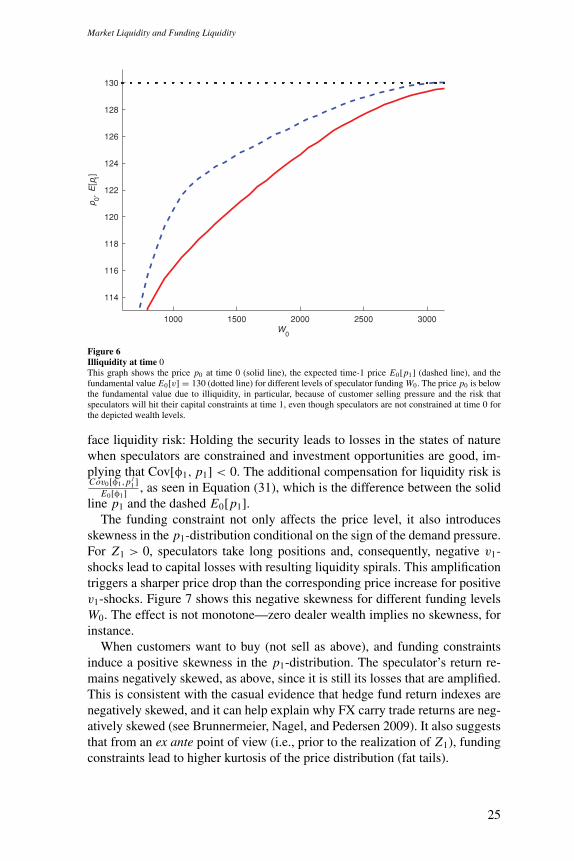
Figure 6 depicts the price p0 and expected time-1 price E0[p1] for differentinitial wealth levels, W0, for which the speculators’ funding constraint is notbinding at t = 0. The figure shows that even though the speculators are un-constrained at time 0, market liquidity provision is limited with prices belowthe fundamental value of E0[v] = 130. The price is below the fundamental fortwo reasons: First, the expected time-1 price is below the fundamental valuebecause of the risk that speculators cannot accommodate the customer sell-ing pressure at that time. Second, p0 is even below E0[p1], since speculators
11 See Brunnermeier (2009) for a more complete treatment of the liquidity and credit crunch that started in 2007.
24
Market Liquidity and Funding Liquidity
1000 1500 2000 2500 3000
114
116
118
120
122
124
126
128
130
W0
p 0, E
[p1]
Figure 6Illiquidity at time 0This graph shows the price p0 at time 0 (solid line), the expected time-1 price E0[p1] (dashed line), and thefundamental value E0[v] = 130 (dotted line) for different levels of speculator funding W0. The price p0 is belowthe fundamental value due to illiquidity, in particular, because of customer selling pressure and the risk thatspeculators will hit their capital constraints at time 1, even though speculators are not constrained at time 0 forthe depicted wealth levels.
face liquidity risk: Holding the security leads to losses in the states of naturewhen speculators are constrained and investment opportunities are good, im-plying that Cov[φ1, p1] < 0. The additional compensation for liquidity risk isCov0[φ1,p j
1 ]E0[φ1] , as seen in Equation (31), which is the difference between the solid
line p1 and the dashed E0[p1].The funding constraint not only affects the price level, it also introduces
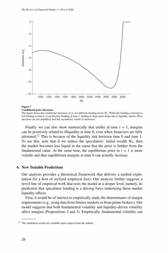
skewness in the p1-distribution conditional on the sign of the demand pressure.For Z1 > 0, speculators take long positions and, consequently, negative v1-shocks lead to capital losses with resulting liquidity spirals. This amplificationtriggers a sharper price drop than the corresponding price increase for positivev1-shocks. Figure 7 shows this negative skewness for different funding levelsW0. The effect is not monotone—zero dealer wealth implies no skewness, forinstance.
When customers want to buy (not sell as above), and funding constraintsinduce a positive skewness in the p1-distribution. The speculator’s return re-mains negatively skewed, as above, since it is still its losses that are amplified.This is consistent with the casual evidence that hedge fund return indexes arenegatively skewed, and it can help explain why FX carry trade returns are neg-atively skewed (see Brunnermeier, Nagel, and Pedersen 2009). It also suggeststhat from an ex ante point of view (i.e., prior to the realization of Z1), fundingconstraints lead to higher kurtosis of the price distribution (fat tails).
25
The Review of Financial Studies / v 00 n 0 2008
1000 1200 1400 1600 1800 2000 2200 2400 2600 2800 3000−12
−10
−8
−6
−4
−2
0
W0
Ske
wne
ss o
f p1
Figure 7Conditional price skewnessThe figure shows the conditional skewness of p1 for different funding levels W0. While the funding constraint isnot binding at time 0, it can become binding at time 1, leading to large price drops due to liquidity spirals. Priceincreases are not amplified, and this asymmetry results in skewness.
Finally, we can also show numerically that unlike at time t = 1, marginscan be positively related to illiquidity at time 0, even when financiers are fullyinformed.12 This is because of the liquidity risk between time 0 and time 1.To see this, note that if we reduce the speculators’ initial wealth W0, thenthe market becomes less liquid in the sense that the price is further from thefundamental value. At the same time, the equilibrium price in t = 1 is morevolatile and thus equilibrium margins at time 0 can actually increase.
6. New Testable Predictions
Our analysis provides a theoretical framework that delivers a unified expla-nation for a host of stylized empirical facts. Our analysis further suggests anovel line of empirical work that tests the model at a deeper level, namely, itsprediction that speculator funding is a driving force underlying these marketliquidity effects.
First, it would be of interest to empirically study the determinants of marginrequirements (e.g., using data from futures markets or from prime brokers). Ourmodel suggests that both fundamental volatility and liquidity-driven volatilityaffect margins (Propositions 2 and 3). Empirically, fundamental volatility can
12 The simulation results are available upon request from the authors.
26
Market Liquidity and Funding Liquidity
be captured using price changes over a longer time period, while the sum offundamental and liquidity-based volatility can be captured by short-term pricechanges as in the literature on variance ratios (see, for example, Campbell,Lo, and MacKinlay 1997). Our model predicts that, in markets where it isharder for financiers to be informed, margins depend on the total fundamentaland liquidity-based volatility. In particular, in times of liquidity crises, marginsincrease in such markets, and, more generally, margins should co-move withilliquidity in the time series and in the cross section.13
Second, our model suggests that an exogenous shock to speculator capitalshould lead to a reduction in market liquidity (Proposition 5). Hence, a cleantest of the model would be to identify exogenous capital shocks, such as anunconnected decision to close down a trading desk, a merger leading to reducedtotal trading capital, or a loss in one market unrelated to the fundamentals ofanother market, and then study the market liquidity and margin around suchevents.
Third, the model implies that the effect of speculator capital on market liq-uidity is highly nonlinear: a marginal change in capital has a small effect whenspeculators are far from their constraints, but a large effect when speculatorsare close to their constraints—illiquidity can suddenly jump (Propositions 4and 5).
Fourth, the model suggests that a cause of the commonality in liquidity isthat the speculators’ shadow cost of capital is a driving state variable. Hence,a measure of speculator capital tightness should help explain the empirical co-movement of market liquidity. Further, our result “commonality of fragility”suggests that especially sharp liquidity reductions occur simultaneously acrossseveral assets (Proposition 6(i)–(ii)).
Fifth, the model predicts that the sensitivity of margins and market liquidityto speculator capital is larger for securities that are risky and illiquid on average.Hence, the model suggests that a shock to speculator capital would lead to areduction in market liquidity through a spiral effect that is stronger for illiquidsecurities (Proposition 6(iv)).
Sixth, speculators are predicted to have negatively skewed returns since,when they hit their constraints, they incur significant losses because of theendogenous liquidity spirals, and, in contrast, their gains are not amplifiedwhen prices return to fundamentals. This leads to conditional skewness andunconditional kurtosis of security prices (Section 5).
7. Conclusion
By linking funding and market liquidity, this paper provides a unified frame-work that explains the following stylized facts:
13 One must be cautious with the interpretation of the empirical results related to changes in Regulation T sincethis regulation may not affect speculators but affects the demanders of liquidity, namely the customers.
27
The Review of Financial Studies / v 00 n 0 2008
(1) Liquidity suddenly dries up; we argue that fragility in liquidity is in partdue to destabilizing margins, which arise when financiers are imperfectlyinformed and the fundamental volatility varies.
(2) Market liquidity and fragility co-moves across assets since changes infunding conditions affects speculators’ market liquidity provision of allassets.
(3) Market liquidity is correlated with volatility, since trading more volatileassets requires higher margin payments and speculators provide marketliquidity across assets such that illiquidity per capital use, i.e., illiquidityper dollar margin, is constant.
(4) Flight to quality phenomena arise in our framework since when fundingbecomes scarce speculators cut back on the market liquidity provisionespecially for capital intensive, i.e., high margin, assets.
(5) Market liquidity moves with the market since funding conditions do.
In addition to explaining these stylized facts, the model also makes a numberof specific testable predictions that could inspire further empirical research onmargins. Importantly, our model links a security’s market illiquidity and riskpremium to its margin requirement (i.e. funding use) and the general shadowcost of funding.
Our analysis also suggests policy implications for central banks. Centralbanks can help mitigate market liquidity problems by controlling funding liq-uidity. If a central bank is better than the typical financiers of speculatorsat distinguishing liquidity shocks from fundamental shocks, then the centralbank can convey this information and urge financiers to relax their fundingrequirements—as the Federal Reserve Bank of New York did during the 1987stock market crash. Central banks can also improve market liquidity by boostingspeculator funding conditions during a liquidity crisis, or by simply stating theintention to provide extra funding during times of crisis, which would loosenmargin requirements as financiers’ worst-case scenarios improve.
Appendix A: Real-World Margin Constraints
A central element of our paper is the capital constraints that the main providers of market liquidityface. In this section, we review the institutional features that drive the funding constraints ofsecurities firms such as hedge funds, banks’ proprietary trading desks, and market makers.
A.1 Funding requirements for hedge fundsWe first consider the funding issues faced by hedge funds since they have relatively simple balancesheets and face little regulation. A hedge fund’s capital consists of its equity capital supplied bythe investors, and possible long-term debt financing that can be relied upon during a potentialfunding crisis. The investors can withdraw their capital at certain times so the equity is not lockedinto the firm indefinitely as in a corporation,14 but, to ensure funding, the withdrawal is subjectto initial lock-up periods and general redemption notice periods before specific redemption dates(typically at least a month, often several months or even years). Also, hedge funds use a variety of
14 A few hedge funds have in fact raised some amount of permanent equity capital.
28
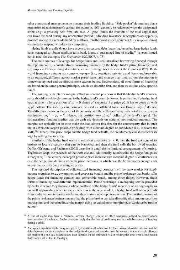
Market Liquidity and Funding Liquidity
other contractual arrangements to manage their funding liquidity: “Side pocket” determines that aproportion of each investor’s capital, for example, 10%, can only be redeemed when the designatedassets (e.g., a privately held firm) are sold. A “gate” limits the fraction of the total capital thatcan leave the fund during any redemption period. Individual investors’ redemptions are typicallyprorated in case of excess demand for outflows. “Withdrawal suspensions” (or force majeure terms)temporarily suspend withdrawals completely.
Hedge funds usually do not have access to unsecured debt financing, but a few large hedge fundshave managed to obtain medium-term bank loans, a guaranteed line of credit,15 or even issuedbonds (see, for example, The Economist 1/27/2007, p. 75).
The main sources of leverage for hedge funds are (i) collateralized borrowing financed throughthe repo market; (ii) collateralized borrowing financed by the hedge fund’s prime broker(s); and(iii) implicit leverage using derivatives, either exchange traded or over the counter (OTC). Real-world financing contracts are complex, opaque (i.e., negotiated privately and hence unobservableto an outsider), different across market participants, and change over time, so our description issomewhat stylized and we discuss some caveats below. Nevertheless, all three forms of financingare based on the same general principle, which we describe first, and then we outline a few specificissues.
The guiding principle for margin setting on levered positions is that the hedge fund’s counter-party should be relatively immune to the hedge fund’s possible losses. In particular, if a hedge fundbuys at time t a long position of x j
t > 0 shares of a security j at price p jt , it has to come up with
x jt p j
t dollars. The security can, however, be used as collateral for a new loan of, say, l jt dollars.
The difference between the price of the security and the collateral value is denoted as the marginrequirement m j+
t = p jt − l j
t . Hence, this position uses x jt m j+
t dollars of the fund’s capital. Thecollateralized funding implies that the cash use depends on margins, not notional amounts. Themargins are typically set so as to make the loan almost risk-free for the counterparty, that is, suchthat it covers the largest possible price drop with a certain degree of confidence (i.e., it covers theVaR).16 Hence, if the price drops and the hedge fund defaults, the counterparty can still recover itsloan by selling the security.
Similarly, if the hedge fund wants to sell short a security, x j < 0, then the fund asks one of itsbrokers to locate a security that can be borrowed, and then the fund sells the borrowed security.Duffie, Garleanu, and Pedersen (2002) describe in detail the institutional arrangements of shorting.The broker keeps the proceeds of the short sale and, additionally, requires that the hedge fund postsa margin m j−
t that covers the largest possible price increase with a certain degree of confidence (incase the hedge fund defaults when the price increases, in which case the broker needs enough cashto buy the security back at a higher price).
This stylized description of collateralized financing portrays well the repo market for fixed-income securities (e.g., government and corporate bonds) and the prime brokerage that banks offerhedge funds for financing equities and convertible bonds, among other things. However, theseforms of financing have different implementation. Prime brokerage is an ongoing service providedby banks in which they finance a whole portfolio of the hedge funds’ securities on an ongoing basis(as well as providing other services), whereas in the repo market, a hedge fund will often get bidsfrom multiple counterparties each time they make a new repo transaction. The portfolio nature ofthe prime brokerage business means that the prime broker can take diversification among securitiesinto account and therefore lower the margin using so-called cross-margining, as we describe furtherbelow.
15 A line of credit may have a “material adverse change” clause or other covenants subject to discretionaryinterpretation of the lender. Such covenants imply that the line of credit may not be a reliable source of fundingduring a crisis.
16 An explicit equation for the margin is given by Equation (6) in Section 1. Often brokers also take into account thedelay between the time a failure by the hedge fund is noticed, and the time the security is actually sold. Hence,the margin of a one-day collateralized loan depends on the estimated risk of holding the asset over a time periodthat is often set as five to ten days.
29
The Review of Financial Studies / v 00 n 0 2008
As an aside, margins on U.S. equities are in principle subject to Regulation T, which stipulatesthat non-brokers/dealers must put down an initial margin (down payment) of 50% of the marketvalue of the underlying stock, both for new long and short positions. Hedge funds can, however,get around Regulation T in various ways and therefore face significantly lower stock margins. Forexample, their prime broker can organize the transaction offshore or as a total return swap, whichis a derivative that is functionally equivalent to buying the stock.
With derivatives, the principle is similar, although the hedge fund does not “borrow against” thesecurity, it must simply post margins to enter into the derivative contract in the first place. Suppose,for instance, that a hedge fund buys an OTC forward contract. The forward contract initially hasa market value of zero (so in this sense the contract has leverage built in), but this does not meanthat you can buy the forward without cash. To enter into the forward contract, which obviouslyhas risk, the hedge fund must post margins corresponding to the largest adverse price move witha certain confidence. To ease netting long and short positions, unwinding, and other things, manyOTC derivatives are structured using standardized swaps provided by the International Swaps andDerivatives Association (ISDA).
For exchange-traded derivatives such as futures and options, a hedge fund trades through aclearing broker (sometimes referred to as a futures clearing merchant). The exchange requiresmargins from the broker, and these margins are set using the same principle as described above,that is, the margin is set to make the exchange almost immune to losses and hence riskier contractshave larger margins. The broker, in turn, typically passes the margin requirement on to the hedgefund. Sometimes, the broker requires higher margins from the hedge fund or lower margins (thelatter is considered granting the hedge fund a risky loan, usually at an interest rate spread). Whilethe broker margins are opaque as mentioned above, the exchange margins are usually publiclyavailable. Figure 1 depicts the exchange margins charged by the CME for the S&P 500 futurescontract.
A hedge fund must finance all of its positions, that is, the sum of all the margin requirementson long and short positions cannot exceed the hedge fund’s capital. In our model, this is capturedby the key Equation (4) in Section 1.
At the end of the financing period, time t + 1, the position is “marked-to-market,” which meansthat the hedge fund is credited any gains (or pays any losses) that have occurred between t andt + 1, that is, the fund receives x j
t (p jt+1 − p j
t ) and pays interest on the loan at the funding rate. Ifthe trade is kept on, the broker keeps the margin to protect against losses going forward from timet + 1. The margin can be adjusted if the risk of the collateral has changed, unless the counterpartieshave contractually fixed the margin for a certain period.
Instead of posting risk-free assets (cash), a hedge fund can also post other risky assets, sayasset k, to cover its margin on position, say x j . However, in this case, a “haircut,” hk
t , is subtractedfrom asset k’s market value to account for the riskiness of the collateral. The funding constraintbecomes x j
t m jt ≤ Wt − xk
t hkt . Moving the haircut term to the left-hand side reveals that the haircut
is equivalent to a margin, since the hedge fund could alternatively have used the risky security toraise cash and then used this cash to cover the margins for asset j . We therefore use the terms“margins” and “haircuts” interchangeably.
We have described how funding constraints work when margins and haircuts are set separatelyfor each security position. As indicated earlier, it is, however, increasingly possible to “cross-margin” (i.e., to jointly finance several positions). This leads to a lower total margin if the risks ofthe various positions are partially offsetting. For instance, much of the interest rate risk is eliminatedin a “spread trade” with a long position in one bond and a short position in a similar bond. Hence,the margin/haircut of a jointly financed spread trade is smaller than the sum of the margins ofthe long and short bonds. For a strategy that is financed jointly, we can reinterpret security j assuch a strategy. Prime brokers compete (especially when credit is as loose as in early 2007) by,among other things, offering low margins and haircuts, a key consideration for hedge funds, whichmeans that it has become increasingly easy to finance more and more strategies jointly. It is by nowrelatively standard to cross-margin an equity portfolio or a portfolio of convertible bonds, and so-called cross-product-margining, which attempts to give diversification benefits across asset classes,
30
Market Liquidity and Funding Liquidity
is becoming more common although it is associated with some issues that make some hedge fundsavoid it.17 In the extreme, one can imagine a joint financing of a hedge fund’s total position suchthat the “portfolio margin” would be equal to the maximum portfolio loss with a certain confidencelevel. Currently, it is often not practical to jointly finance a large portfolio with all the benefitsof diversification. This is because a large hedge fund finances its trades using several brokers;both a hedge fund and a broker can consist of several legal entities (possibly located in differentjurisdictions); certain trades need separate margins paid to exchanges (e.g., futures and options) orto other counterparties of the prime broker (e.g., securities lenders); prime brokers may not havesufficiently sophisticated models to evaluate the diversification benefits (e.g., because they do nothave enough data on the historical performance of newer products such as CDOs); and becauseof other practical difficulties in providing joint financing. Further, if the margin requirement relieson assumed stress scenarios in which the securities are perfectly correlated (e.g., due to predatorytrading, as in Brunnermeier and Pedersen 2005), then the portfolio margin constraint coincideswith position-by-position margins.
A.2 Funding requirements for commercial and investment banksA bank’s capital consists of equity capital plus its long-term borrowing (including credit linessecured from commercial banks, alone or in syndicates), reduced by assets that cannot be read-ily employed (e.g., goodwill, intangible assets, property, equipment, and capital needed for dailyoperations), and further reduced by uncollateralized loans extended by the bank to others (see,for example, Goldman Sachs’s 2003 Annual Report). Banks also raise money using short-termuncollateralized loans, such as commercial paper and promissory notes, and, in the case of com-mercial banks, demand deposits. These sources of financing cannot, however, be relied on in timesof funding crisis since lenders may be unwilling to continue lending, and therefore this short-termfunding is often not included in measures of capital.
The financing of a bank’s trading activity is largely based on collateralized borrowing. Bankscan finance long positions using collateralized borrowing from corporations, other banks, insurancecompanies, and the Federal Reserve Bank, and can borrow securities to short-sell from, for instance,mutual funds and pension funds. These transactions typically require margins that must be financedby the bank’s capital, as captured by the funding constraint in Equation (4).
The financing of a bank’s trading is more complicated than that of a hedge fund, however.For instance, banks may negotiate zero margins with certain counterparties, and banks can oftensell short shares held in-house, that is, held in a customer’s margin account (in “street name”)such that the bank does not need to use capital to borrow the shares externally. Further, a bankreceives margins when financing hedge funds (i.e., the margin is negative from the point of viewof the bank). In spite of these caveats, in times of stress, banks face margin requirements and areultimately subject to a funding constraint in the spirit of Equation (4). Bear Stearns’s demise is avivid reminder that banks’ funding advantage from clients’ margin accounts can quickly evaporate.In March of 2008, Bear Stearns’s clients terminated their brokerage relationships and ran on theinvestment bank. Only an orchestrated merger with JPMorgan Chase avoided a bankruptcy.
Banks must also satisfy certain regulatory requirements. Commercial banks are subject to theBasel Accord, supervised by the Federal Reserve System for U.S. banks. In short, the Basel Accordof 1988 requires that a bank’s “eligible capital” exceeds 8% of the “risk-weighted asset holdings,”which is the sum of each asset holding multiplied by its risk weight. The risk weight is 0% for cashand government securities, 50% for mortgage-backed loans, and 100% for all other assets. Therequirement posed by the 1988 Basel Accord corresponds to Equation (4) with margins of 0%, 4%,and 8%, respectively. In 1996, the accord was amended, allowing banks to measure market riskusing an internal model based on portfolio VaRs rather than using standardized risk weights. To
17 For instance, cross-product margining means that the broker effectively can move extra cash from one marginaccount to cover a loss elsewhere, even if the hedge may dispute the loss. Also, collecting all positions with onebroker may mean that the hedge fund cannot get a good pricing on the trades, e.g., on repos, and may expose thehedge fund to predatory trading.
31
The Review of Financial Studies / v 00 n 0 2008
outmaneuver the Basel Accord, banks created a shadow banking system, which allowed them tooff-load assets to off-balance sheet vehicles like SIVs and conduits. For details, see Brunnermeier(2009).
Broker-speculators in the United States, including banks acting as such, are subject to theSecurities and Exchange Commission’s (SEC’s) “net capital rule” (SEC Rule 15c3-1). This rulestipulates, among other things, that a broker must have a minimum “net capital,” which is definedas equity capital plus approved subordinate liabilities minus “securities haircuts” and operationalcharges. The haircuts are set as security-dependent percentages of the market value. The standardrule requires that the net capital exceeds at least 6 2
3 % (15:1 leverage) of aggregate indebtedness(broker’s total money liabilities) or alternatively 2% of aggregate debit items arising from customertransactions. This constraint is similar in spirit to Equation (4).18 As of August 20, 2004, SECamended the net capital rule for Consolidated Supervised Entities (CSEs) such that CSEs may,under certain circumstances, use their internal risk models to determine whether they fulfill theircapital requirement (SEC Release No. 34-49830).
A.3 Funding requirements for market makersThere are various types of market-making firms. Some are small partnerships, whereas others areparts of large investment banks. The small firms are financed in a similar way to hedge funds in thatthey rely primarily on collateralized financing; the funding of banks was described in Section A2.
Certain market makers, such as NYSE specialists, have an obligation to make a market; anda binding funding constraint means that they cannot fulfill this requirement. Hence, avoiding thefunding constraint is especially crucial for such market makers.
Market makers are in principle subject to the SEC’s net capital rule (described in Section A2),but this rule has special exceptions for market makers. Hence, market makers’ main regulatoryrequirements are those imposed by the exchange on which they operate. These constraints are oftensimilar in spirit to Equation (4).
Appendix B: Proofs
Proof of Propositions 1–3These results follow from the calculations in the text.
Proof of Proposition 4We prove the proposition for Z1 > 0, implying p1 ≤ v1 and x1 ≥ 0. The complementary case isanalogous. To see how the equilibrium depends on the exogenous shocks, we first combine theequilibrium condition x1 = −∑1
k=0 yk1 with the speculator funding constraint to get
m+1
(Z1 − 2
γ(σ2)2(v1 − p1)
)≤ b0 + p1x0 + η1, (B1)
that is,
G(p1) := m+1
(Z1 − 2
γ(σ2)2(v1 − p1)
)− p1x0 − b0 ≤ η1. (B2)
For η1 large enough, this inequality is satisfied for p1 = v1, that is, it is a stable equilibrium thatthe market is perfectly liquid. For η1 low enough, the inequality is violated for p1 = 2v1
γ(σ2)2 − Z1,
that is, it is an equilibrium that the speculator is in default. We are interested in intermediate values
18 Let L be the lower of 6 23 % of total indebtedness or 2% of debit items and h j the haircut for security j ; then the
rule requires that L ≤ W −∑ j h j x j , that is,∑
j h j x j ≤ W − L .
32
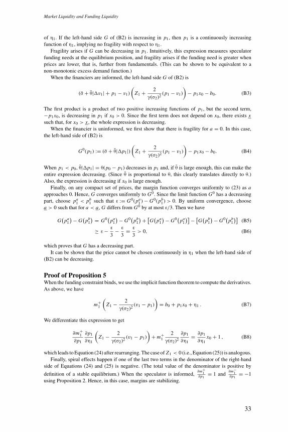
Market Liquidity and Funding Liquidity
of η1. If the left-hand side G of (B2) is increasing in p1, then p1 is a continuously increasingfunction of η1, implying no fragility with respect to η1.
Fragility arises if G can be decreasing in p1. Intuitively, this expression measures speculatorfunding needs at the equilibrium position, and fragility arises if the funding need is greater whenprices are lower, that is, further from fundamentals. (This can be shown to be equivalent to anon-monotonic excess demand function.)
When the financiers are informed, the left-hand side G of (B2) is
(σ + θ|�v1| + p1 − v1)
(Z1 + 2
γ(σ2)2(p1 − v1)
)− p1x0 − b0. (B3)
The first product is a product of two positive increasing functions of p1, but the second term,−p1x0, is decreasing in p1 if x0 > 0. Since the first term does not depend on x0, there exists xsuch that, for x0 > x , the whole expression is decreasing.
When the financier is uninformed, we first show that there is fragility for a = 0. In this case,the left-hand side of (B2) is
G0(p1) := (σ + θ|�p1|)(
Z1 + 2
γ(σ2)2(p1 − v1)
)− p1x0 − b0. (B4)
When p1 < p0, θ|�p1| = θ(p0 − p1) decreases in p1 and, if θ is large enough, this can make theentire expression decreasing. (Since θ is proportional to θ, this clearly translates directly to θ.)Also, the expression is decreasing if x0 is large enough.
Finally, on any compact set of prices, the margin function converges uniformly to (23) as aapproaches 0. Hence, G converges uniformly to G0. Since the limit function G0 has a decreasingpart, choose pa
1 < pb1 such that ε := G0(pa
1 ) − G0(pb1 ) > 0. By uniform convergence, choose
a > 0 such that for a < a, G differs from G0 by at most ε/3. Then we have
G(
pa1
)− G(
pb1
) = G0(pa1
)− G0(pb1
)+ [G(pa1
)− G0(pa1
)]− [G(pb1
)− G0(pb1
)](B5)
≥ ε − ε
3− ε
3= ε
3> 0, (B6)
which proves that G has a decreasing part.It can be shown that the price cannot be chosen continuously in η1 when the left-hand side of
(B2) can be decreasing.
Proof of Proposition 5When the funding constraint binds, we use the implicit function theorem to compute the derivatives.As above, we have
m+1
(Z1 − 2
γ(σ2)2(v1 − p1)
)= b0 + p1x0 + η1 . (B7)
We differentiate this expression to get
∂m+1
∂p1
∂p1
∂η1
(Z1 − 2
γ(σ2)2(v1 − p1)
)+ m+
12
γ(σ2)2
∂p1
∂η1= ∂p1
∂η1x0 + 1 , (B8)
which leads to Equation (24) after rearranging. The case of Z1 < 0 (i.e., Equation (25)) is analogous.Finally, spiral effects happen if one of the last two terms in the denominator of the right-hand
side of Equations (24) and (25) is negative. (The total value of the denominator is positive by
definition of a stable equilibrium.) When the speculator is informed,∂m+
1∂p1
= 1 and∂m−
1∂p1
= −1using Proposition 2. Hence, in this case, margins are stabilizing.
33
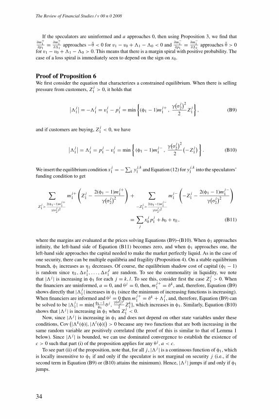
The Review of Financial Studies / v 00 n 0 2008
If the speculators are uninformed and a approaches 0, then using Proposition 3, we find that∂m+
1∂p1
= ∂m+1
∂�1approaches −θ < 0 for v1 − v0 + �1 − �0 < 0 and
∂m−1
∂p1= ∂m−
1∂�1
approaches θ > 0for v1 − v0 + �1 − �0 > 0. This means that there is a margin spiral with positive probability. Thecase of a loss spiral is immediately seen to depend on the sign on x0.
Proof of Proposition 6We first consider the equation that characterizes a constrained equilibrium. When there is sellingpressure from customers, Z j
1 > 0, it holds that
∣∣� j1
∣∣ = −�j1 = v
j1 − p j
1 = min
{(φ1 − 1)m j+
1 ,γ(σ
j2
)22
Z j1
}, (B9)
and if customers are buying, Z j1 < 0, we have
∣∣� j1
∣∣ = �j1 = p j
1 − vj1 = min
{(φ1 − 1)m j−
1 ,γ(σ
j2
)22
(−Z j1
) }. (B10)
We insert the equilibrium condition x j1 = −∑k y j,k
1 and Equation (12) for y j,k1 into the speculators’
funding condition to get
∑Z j
1 >2(φ1−1)m
j+1
γ(σj2 )2
m j+1
(Z j
1 − 2(φ1 − 1)m j+1
γ(σ
j2
)2)
+∑
−Z j1 >
2(φ1−1)mj−1
γ(σj2 )2
m j−1
(−Z j
1 − 2(φ1 − 1)m j−1
γ(σ
j2
)2)
=∑
j
x j0 p j
1 + b0 + η1, (B11)
where the margins are evaluated at the prices solving Equations (B9)–(B10). When φ1 approachesinfinity, the left-hand side of Equation (B11) becomes zero, and when φ1 approaches one, theleft-hand side approaches the capital needed to make the market perfectly liquid. As in the case ofone security, there can be multiple equilibria and fragility (Proposition 4). On a stable equilibriumbranch, φ1 increases as η1 decreases. Of course, the equilibrium shadow cost of capital (φ1 − 1)is random since η1, �v1
1 , . . . , �v J1 are random. To see the commonality in liquidity, we note
that |� j | is increasing in φ1 for each j = k, l. To see this, consider first the case Z j1 > 0. When
the financiers are uninformed, a = 0, and θ j = 0, then, m j+1 = σk , and, therefore, Equation (B9)
shows directly that |� j1 | increases in φ1 (since the minimum of increasing functions is increasing).
When financiers are informed and θ j = 0 then m j+1 = σk + �
j1, and, therefore, Equation (B9) can
be solved to be |� j1 | = min{ φ1−1
φ1σ j ,
γ(σk2)2
2 Zk1}, which increases in φ1. Similarly, Equation (B10)
shows that |� j | is increasing in φ1 when Z j1 < 0.
Now, since |� j | is increasing in φ1 and does not depend on other state variables under theseconditions, Cov
(|�k (φ)|, |�l (φ)|) > 0 because any two functions that are both increasing in thesame random variable are positively correlated (the proof of this is similar to that of Lemma 1below). Since |� j | is bounded, we can use dominated convergence to establish the existence ofc > 0 such that part (i) of the proposition applies for any θ j , a < c.
To see part (ii) of the proposition, note that, for all j , |� j | is a continuous function of φ1, whichis locally insensitive to φ1 if and only if the speculator is not marginal on security j (i.e., if thesecond term in Equation (B9) or (B10) attains the minimum). Hence, |� j | jumps if and only if φ1
jumps.
34
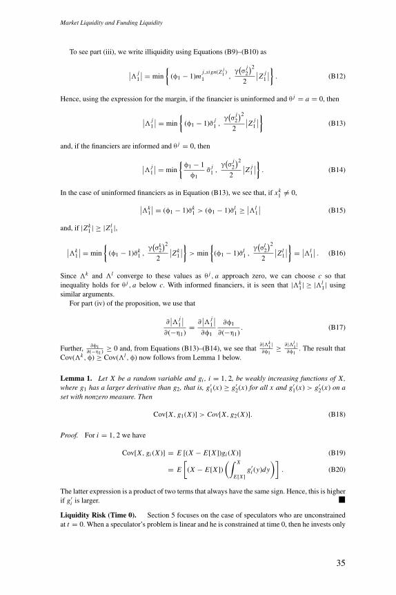
Market Liquidity and Funding Liquidity
To see part (iii), we write illiquidity using Equations (B9)–(B10) as
∣∣� j1
∣∣ = min
{(φ1 − 1)m
j,sign(Z j1 )
1 ,γ(σ
j2
)22
∣∣Z j1
∣∣} . (B12)
Hence, using the expression for the margin, if the financier is uninformed and θ j = a = 0, then
∣∣� j1
∣∣ = min
{(φ1 − 1)σ j
1 ,γ(σ
j2
)22
∣∣Z j1
∣∣} (B13)
and, if the financiers are informed and θ j = 0, then
∣∣� j1
∣∣ = min
{φ1 − 1
φ1σ
j1 ,
γ(σ
j2
)22
∣∣Z j1
∣∣} . (B14)
In the case of uninformed financiers as in Equation (B13), we see that, if xk1 �= 0,
∣∣�k1
∣∣ = (φ1 − 1)σk1 > (φ1 − 1)σl
1 ≥ ∣∣�l1
∣∣ (B15)
and, if |Zk1 | ≥ |Zl
1|,
∣∣�k1
∣∣ = min
{(φ1 − 1)σk
1 ,γ(σk
2
)22
∣∣Zk1
∣∣} > min
{(φ1 − 1)σl
1 ,γ(σl
2
)22
∣∣Zl1
∣∣} = ∣∣�l1
∣∣ . (B16)
Since �k and �l converge to these values as θ j , a approach zero, we can choose c so thatinequality holds for θ j , a below c. With informed financiers, it is seen that |�k
1| ≥ |�l1| using
similar arguments.For part (iv) of the proposition, we use that
∂∣∣� j
1
∣∣∂(−η1)
= ∂∣∣� j
1
∣∣∂φ1
∂φ1
∂(−η1). (B17)
Further, ∂φ1∂(−η1) ≥ 0 and, from Equations (B13)–(B14), we see that
∂|�k1 |
∂φ1≥ ∂|�l
1|∂φ1
. The result thatCov(�k , φ) ≥ Cov(�l , φ) now follows from Lemma 1 below.
Lemma 1. Let X be a random variable and gi , i = 1, 2, be weakly increasing functions of X,where g1 has a larger derivative than g2, that is, g′
1(x) ≥ g′2(x) for all x and g′
1(x) > g′2(x) on a
set with nonzero measure. Then
Cov[X, g1(X )] > Cov[X, g2(X )]. (B18)
Proof. For i = 1, 2 we have
Cov[X, gi (X )] = E [(X − E[X ])gi (X )] (B19)
= E
[(X − E[X ])
(∫ X
E[X ]g′
i (y)dy
)]. (B20)
The latter expression is a product of two terms that always have the same sign. Hence, this is higherif g′
i is larger. �Liquidity Risk (Time 0). Section 5 focuses on the case of speculators who are unconstrainedat t = 0. When a speculator’s problem is linear and he is constrained at time 0, then he invests only
35
The Review of Financial Studies / v 00 n 0 2008
in securities with the highest expected profit per capital use, where profit is calculated using thepricing kernel φi
1/E0[φi1]. In this case, his time-0 shadow cost of capital is
φi0 = E0[φi
1]
⎧⎪⎨⎪⎩1 + max
j
⎛⎜⎝ E0
[ φi1
E0[φi1]
p j1
]− p j0
m+0
, −E0[ φi
1E0[φi
1]p j
1
]− p j0
m−0
⎞⎟⎠⎫⎪⎬⎪⎭ . (B21)
ReferencesAbreu, D., and M. K. Brunnermeier. 2002. Synchronization Risk and Delayed Arbitrage. Journal of FinancialEconomics 66:341–60.
Acharya, V. V., and L. H. Pedersen. 2005. Asset Pricing with Liquidity Risk. Journal of Financial Economics77:375–410.
Acharya, V. V., S. Schaefer, and Y. Zhang. 2008. Liquidity Risk and Correlation Risk: A Clinical Study of theGeneral Motors and Ford Downgrade of 2005. Working Paper, London Business School.
Adrian, T., and H. S. Shin. 2009. Liquidity and Leverage. Journal of Financial Intermediation.
Aiyagari, S. R., and M. Gertler. 1999. “Overreaction” of Asset Prices in General Equilibrium. Review of EconomicDynamics 2:3–35.
Allen, F., and D. Gale. 1998. Optimal Financial Crisis. Journal of Finance 53:1245–84.
Allen, F., and D. Gale. 2004. Financial Intermediaries and Markets. Econometrica 72:1023–61.
Allen, F., and D. Gale. 2005. Financial Fragility, Liquidity, and Asset Prices. Journal of the European EconomicAssociation 2:1015–48.
Allen, F., and D. Gale. 2007. Understanding Financial Crises. Clarendon Lectures in Economics. Oxford, UK:Oxford University Press.
Amihud, Y., and H. Mendelson. 1989. The Effects of Beta, Bid-Ask Spread, Residual Risk, and Size on StockReturns. Journal of Finance 44:479–86.
Attari, M., A. S. Mello, and M. E. Ruckes. 2005. Arbitraging Arbitrageurs. Journal of Finance 60:2471–511.
Benston, G. J., and R. L. Hagerman. 1974. Determinants of the Bid-Ask Spread in the Over-the-Counter Market.Journal of Financial Economics 1:353–64.
Bernanke, B., and M. Gertler. 1989. Agency Costs, Net Worth, and Business Fluctuations. American EconomicReview 79:14–31.
Bernardo, A. E., and I. Welch. 2004. Liquidity and Financial Markets Run. Quarterly Journal of Economics119:135–58.
Brunnermeier, M. K. 2009. Deciphering the Liquidity and Credit Crunch 2007–08. Journal of Economic Per-spectives. 2009, Issue 1.
Brunnermeier, M. K., S. Nagel, and L. H. Pedersen. 2009. Carry Trades and Currency Crashes, in DaronAcemoglu, Kenneth Rogoff, and Michael Woodford (eds.), NBER Macroeconomics Annual 2008, vol. 23.Cambridge, MA: MIT Press.
Brunnermeier, M. K., and L. H. Pedersen. 2005. Predatory Trading. Journal of Finance 60:1825–63.
Bryant, J. 1980. A Model of Reserves, Bank Runs, and Deposit Insurance. Journal of Banking and Finance4:335–44.
Campbell, J. Y., A. W. Lo, and A. C. MacKinlay. 1997. The Econometrics of Financial Markets. Princeton, NJ:Princeton University Press.
36
Market Liquidity and Funding Liquidity
Chordia, T., R. Roll, and A. Subrahmanyam. 2000. Commonality in Liquidity. Journal of Financial Economics56:3–28.
Chordia, T., A. Sarkar, and A. Subrahmanyam. 2005. An Empirical Analysis of Stock and Bond Market Liquidity.Review of Financial Studies 18:85–129.
Chowdhry, B., and V. Nanda. 1998. Leverage and Market Stability: The Role of Margin Rules and Price Limits.Journal of Business 71:179–210.
Comerton-Forde, C., T. Hendershott, C. M. Jones, P. C. Moulton, and M. S. Seasholes. 2008. Time Variation inLiquidity: The Role of Market Maker Inventories and Revenues. Working Paper, Columbia University.
Coughenour, J. F., and M. M. Saad. 2004. Common Market Makers and Commonality in Liquidity. Journal ofFinancial Economics 73:37–69.
DeLong, J. B., A. Shleifer, L. H. Summers, and R. J. Waldmann. 1990. Noise Trader Risk in Financial Markets.Journal of Political Economy 98:703–38.
Diamond, D., and P. Dybvig. 1983. Bank Runs, Deposit Insurance, and Liquidity. Journal of Political Economy91:401–19.
Duffie, D., N. Garleanu, and L. H. Pedersen. 2002. Securities Lending, Shorting, and Pricing. Journal of FinancialEconomics 66:307–39.
Eisfeldt, A. 2004. Endogenous Liquidity in Asset Markets. Journal of Finance 59:1–30.
Fisher, I. 1933. The Debt-Deflation Theory of Great Depression. Econometrica 1:337–57.
Fostel, A., and J. Geanakoplos. 2008. Leverage Cycles and The Anxious Economy. American Economic Review98:1211–44.
Garleanu, N., and L. H. Pedersen. 2007. Liquidity and Risk Management. The American Economic Review(Papers & Proceedings) 97:193–97.
Garleanu, N., L. H. Pedersen, and A. Poteshman. 2008. Demand-Based Option Pricing. Review of FinancialStudies.
Geanakoplos, J. 1997. Promises, Promises in W.B. Arthur, S. Durlauf and D. Lane (eds.), The Economy as anEvolving Complex System II 1997: 285–320. Addison-Wesley, Reading MA.
Geanakoplos, J. 2003. Liquidity, Default and Crashes: Endogenous Contracts in General Equilibrium, in MathiasDewatripont, Lars Peter Hansen, and Stephen J. Turnovsky (eds.), Advances in Economics and Econometrics:Theory and Applications II, Eighth World Congress, vol. 2, pp. 170–205. Econometric Society Monographs.Cambridge, UK: Cambridge University Press.
Gennotte, G., and H. Leland. 1990. Market Liquidity, Hedging, and Crashes. American Economic Review80:999–1021.
Glosten, L. R., and P. R. Milgrom. 1985. Bid, Ask, and Transaction Prices in a Specialist Market with Heteroge-neously Informed Traders. Journal of Financial Economics 14:71–100.
Gromb, D., and D. Vayanos. 2002. Equilibrium and Welfare in Markets with Financially Constrained Arbi-trageurs. Journal of Financial Economics 66:361–407.
Grossman, S. J. 1988. An Analysis of the Implications for Stock and Futures Price Volatility of Program Tradingand Dynamic Hedging Strategies. Journal of Business 61:275–98.
Grossman, S. J., and M. H. Miller. 1988. Liquidity and Market Structure. Journal of Finance 43:617–33.
Grossman, S. J., and J.-L. Vila. 1992. Optimal Dynamic Trading with Leverage Constraints. Journal of Financialand Quantitative Analysis 27:151–68.
Hameed, A., W. Kang, and S. Viswanathan. 2005. Asymmetric Comovement in Liquidity. Mimeo, DukeUniversity.
37
The Review of Financial Studies / v 00 n 0 2008
Hasbrouck, J., and D. Seppi. 2001. Common Factors in Prices, Order Flows, and Liquidity. Journal of FinancialEconomics 59:383–411.
Ho, T. S. Y., and H. R. Stoll. 1981. Optimal Dealer Pricing under Transactions and Return Uncertainty. Journalof Financial Economics 9:47–73.
Ho, T. S. Y., and H. R. Stoll. 1983. The Dynamics of Dealer Markets under Competition. Journal of Finance38:1053–74.
Holmstrom, B., and J. Tirole. 1998. Private and Public Supply of Liquidity. Journal of Political Economy106:1–39.
Holmstrom, B., and J. Tirole. 2001. LAPM: A Liquidity-Based Asset Pricing Model. Journal of Finance56:1837–67.
Huberman, G., and D. Halka. 2001. Systematic Liquidity. Journal of Financial Research 24:161–78.
Ibbotson. 1999. Cost of Capital Quarterly, 1999 Yearbook, 2nd ed. Chicago: Ibbotson Associates, 1976.
International Monetary Fund. 2007. Global Financial Stability Report. October.
Kiyotaki, N., and J. Moore. 1997. Credit Cycles. Journal of Political Economy 105:211–48.
Kyle, A. S. 1985. Continuous Auctions and Insider Trading. Econometrica 53:1315–35.
Kyle, A. S., and W. Xiong. 2001. Contagion as a Wealth Effect. Journal of Finance 56:1401–40.
Liu, J., and F. A. Longstaff. 2004. Losing Money on Arbitrages: Optimal Dynamic Portfolio Choice in Marketswith Arbitrage Opportunities. Review of Financial Studies 17:611–41.
Lustig H., and Y. Chien. 2005. The Market Price of Aggregate Risk and Wealth Distribution. NBER WorkingPaper 11132.
Mitchell, M., L. H. Pedersen, and T. Pulvino. 2007. Slow Moving Capital. American Economic Review (Papers& Proceedings) 97:215–20.
Morris, S., and H. Shin. 2004. Liquidity Black Holes. Review of Finance 8:1–18.
Pastor, L., and R. F. Stambaugh. 2003. Liquidity Risk and Expected Stock Returns. Journal of Political Economy111:642–85.
Plantin, G., H. Sapra, and H. S. Shin. 2005. Marking-to-Market: Panacea or Pandora’s Box? Journal of AccountingResearch 46:435–60.
Shleifer, A., and R. W. Vishny. 1992. Liquidation Values and Debt Capacity: A Market Equilibrium Approach.Journal of Finance 47:1343–66.
Shleifer, A., and R. W. Vishny. 1997. The Limits of Arbitrage. Journal of Finance 52:35–55.
Stiglitz, J. E., and A. Weiss. 1981. Credit Rationing in Markets with Imperfect Information. American EconomicReview 71:393–410.
Stoll, H. R. 1978. The Supply of Dealer Services in Securities Markets. Journal of Finance 33:1133–51.
Vayanos, D. 2004. Flight to Quality, Flight to Liquidity, and the Pricing of Risk. Working Paper, London Schoolof Economics.
Weill, P.-O. 2007. Leaning Against the Wind. Review of Economic Studies 74:1329–54.
Wigmore, B. 1998. Revisiting the October 1987 Crash. Financial Analysts Journal 54:36–48.
Xiong, W. 2001. Convergence Trading with Wealth Effects: An Amplification Mechanism in Financial Markets.Journal of Financial Economics 62(2): 247–92.
38