Market Failure: Public Goods and ExternalitiesLecture notes

Dan Anderberg

Royal Holloway University of London

January 2007

1 Introduction

One justification for government intervention is market failures. With market failures the

first theorem of welfare economics breaks down and the decentralized market equilibrium

will fail to be Pareto optimal. There may then be a government intervention to improve

efficiency.

In this lecture we will consider two particular types of market failures: public goods

and externalities. No doubt you are all aware of what we mean by public goods and

externalities, so I assume that the topics need very little introduction. We will start by

looking a public goods. So what will we be saying about public goods?

2 Public Goods: An Overview

The fundamental problem with public goods is how to design institutions such that

maximum efficiency obtains. We might want to consider question such as: How bad is the

market mechanism? Can other institutions be designed that generate better allocations?

Our first tasks are thus as follows:

• Establish benchmark case: Characterize Pareto optimal allocations

• Consider institutions that determine public good provision:

— Voluntary provision

— Collective action, voting.

1

We will consider what happens when the consumers make voluntary contributions to

a public good; this is effectively the competitive market equilibrium. As we will see there

will be a substantial free rider problem. It is frequently argued that public goods ought

to be publicly provided. If so, one can imagine either that the provision problem is solved

by a benevolent policy maker (in which case we can expect the policy maker to select a

Pareto optimal allocation); alternatively, one can imagine that the provision problem is

determined through collective action e.g. through a democratic process such as majority

voting. Hence we will consider the outcome of majority voting.

We will also consider extensions of the pure public goods model that are of great

practical importance: These include congestion, “club goods”, “local public goods”. The

theory of local public goods has recently been on the research agenda, because it can

be used to study a range of interesting phenomena. In the US debate, a big debate is

e.g. schooling and segregation; in Europe the theory of local public goods has become

important for the study of European integration.

A fundamental problem associate with public goods is that the consumers do not have

the incentives to reveal their preferences; this is what causes free-riding in the market

equilibrium. It is also what causes inefficiencies associated with voting. This raises the

question if there is any way to design mechanisms for determining public good supply

which provide the consumers the incentives to truthfully reveal their preferences. Hence

we will briefly consider the whether and how one can design mechanism to reveal the

individuals’ preferences.

The preference-revelation problem was very much on the research agenda a decade

or two ago. What emerged from that research was that it is possible to come up with

well designed mechanisms whereby each consumer would, in fact, have an incentive to

truthfully reveal their incentives. However, the mechanisms also have limitations.

2

3 Public Goods: Pareto Efficiency

3.1 Characterizing Features

So far we have been considering private goods; private goods have two characterizing

features. The first is that there is rivalry among consumers in the sense that consumption

by one consumer reduces the amount available to others. The second characterizing

feature is that private goods are subject to exclusion — one has to own a good in order

to consume it: it if is not yours you are effectively prevented from enjoying it. The

characterizing feature of a pure public good is, on the other hand, the exact opposite.

Definition 1 Non-rivalry. Consumption of a good by one consumer does not reduce the

amount available to other consumers.

Definition 2 Non-excludability. If a good is supplied, then no consumer can be excluded

from consuming it.

Definition 3 A pure public good has both the non-rivalry property and the non-excludability

property.

However, some goods are non-rivalrous but still excludable. Consider e.g. a bridge:

assuming that there is no congestion it is non-rivalrous; it is nevertheless easy to exclude

consumers from using it. Some goods, may partially fail the non-rivalry property; in that

case we say that there is congestion. Congestion will be important when we consider club

goods.

3.2 The Samuelson Rule

The first logical step is to characterize the efficient allocation. Thus consider the following

economy. There is a set of consumers i ∈ I = {1, 2, ..., n}. There is one private goodx and one public good z. The assumption that there is only one public good and one

private good is made for simplicity — the extension to several goods of each type is

straightforward. Consumer i’s preferences are represented by a utility function ui (xi, zi).

Each consumer is assumed to have strictly convex and strictly monotonic preferences.

3

We can use a simple production function formulation to summarize the economy’s

technology. Hence suppose that the public good z is produced using the private good

as input. Let the technology be summarized by z = f (x) where f is strictly increasing,

continuous, and (weakly) concave and where x is the amount of the private goods used

as input in the production the public good.

Let there be an initial aggregate endowment ωx units of x.[FIX] Also let we use the

vector notation x = (xi)i∈I to denote the describe the level of consumption of the private

good by each consumer; thus x a vector of length n. Similarly let z = (zi)i∈I describe

the level of consumption of the private good by each consumer. Note that we are not

assuming that each consumer will automatically consume the same amount; rather we

will impose as feasibility constraint the each consumer consumes at most f (x) of the

public good, i.e. the amount produced.

Definition 4 An allocation is a pair (x, z).

Consider the feasibility constraints for this economy.

Definition 5 An allocation (x, z) is feasible ifXi∈Ixi ≤ ωx − x, and (1)

zi ≤ f (x) for all i ∈ I. (2)

The second constraint captures the non-rivalry of z. In principle, a consumer can

consume less than the available amount of z, zi ≤ f (x). However, since preferences

are strongly monotone, this will never be efficient. Hence, given that we are seeking to

characterize efficient allocation, we can focus on zi = z = f (x) for all i ∈ I.Pareto optimal allocations can be characterized as the solution to an optimization

problem. In particular, consider the problem of maximizing the utility of individual i

given a set of required utilities for the other individuals and given the aggregate resource

constraint.

Figure 3.1 illustrate the case where there are two consumers; for a given level of utility

to individual 1, denoted u1, we maximize the utility of individual 2 given the feasibility

4

constraint. The value of that problem is the value of the utility possibility frontier at

that specific value of u1. Then as we vary the required utility for individual 1 we trace

out the utility possibility frontier (UPF).

FIG 3.1

When we have n individuals we fix the utility for all individuals except one, individual

i, and maximize the utility of this last individual subject to the fixed utility for everyone

else and subject to the feasibility constraint. Letting g (·) be the inverse of f (·), g (z)measures the amount of the private goods required as input in order to produce z units

of the public good; using this we can simplify the feasibility constraint to the inequalityPi∈I xi ≤ ωx − g (z) (which allows us to eliminate the input level x from the feasibility

constraint).

Pareto optimality can then be characterize as follows:

Lemma 1 A feasible allocation (x∗, z∗) is Pareto optimal if and only if it solves the fol-

lowing problem for every i ∈ I

maxx,z ui (xi, z)

s.t. uj¡x∗j , z

∗¢ ≤ uj (xj , z) , j 6= i (γi)

andP

i∈I xi ≤ ωx − g (z) (λ)

(3)

Note that in this problem we have as utility requirements for the “other individuals” the

utilities that they enjoy at the Pareto optimal allocation (x∗, z∗). The Lagrangean for this

problem, for i = 1 (say)

L = u1 (x1, z)− γj

nXi=2

£uj¡x∗j , z

∗¢− uj (xj, z)¤− λ

"Xi∈Ixi − ωx + g (z)

#.

Since (x∗, z∗) is a solution to (3), by the Kuhn-Tucker theorem, there exists¡γ∗j¢nj=2

and λ∗ such that all derivatives of L are zero at (x∗, z∗,γ∗,λ∗). If we also define γ∗1 ≡ 1we can write the first-order conditions

∂L∂xi

= γ∗i∂ui∂xi− λ∗ = 0, i ∈ I (4)

∂L∂z

=Xi∈I

γ∗i∂ui∂z− λ∗g0 (z∗) = 0. (5)

5

Solving (4) for γ∗i and then substituting in (5) we can eliminate the multiplier: this yields

Xi∈I

∂ui/∂z

∂ui/∂xi= g0 (z∗) (Samuelson Condition). (6)

The interpretation of the Samuelson (1954, 1955) condition is straightforward. Note

that

∂ui/∂z

∂ui/∂xi

can be interpreted as consumer i’s marginal willingness to pay for z (in terms of the

private good), i.e. the individual’s marginal rate of substitution. The right hand side of

(6) measures the marginal cost of z (again in terms of the private good) — the marginal rate

of transformation. Hence the condition states that the sum of the consumers’ marginal

willingness to pay for z should equal the marginal cost.

Note that the Samuelson rule does not rely on non-excludability, only non-rivalry.

Simply — since the good is non-rivalrous, and since the consumers have monotone pref-

erences optimality requires that no one is excluded, so whether exclusion is possible is

irrelevant — it would never be optimal. However, excludability may become important

when we consider different institutions for determining public good supply.

4 Equilibria with Private Provision of Public Goods

If there was a benevolent government with unrestricted policy instruments and perfect

information about preferences, then we would expect the Samuelson rule to be imple-

mented. However, suppose instead that there is no government at all, but only a private

market. On that private market each consumer can buy units of the public good; since

the public good is non-excludable if a consumer does decide to buys some amount of

the private good, that amount will automatically be available to all other consumers as

well. This suggests that there may be free riding: every consumer would happy to enjoy

the contributions to the public good done by other and would be less inclined to make

own contributions. A natural conjecture would thus be that there will be too little vol-

untary public good provision. Moreover, we would expect that problem to be worse in

6

large economies than in small economies. Thus let’s consider private provision equilibria

formally.

In order to do so, let’s modify the model a little bit. We will do this in order to bring

in “individual incomes” into the model. One factor of production (labour) is supplied

inelastically by each consumer; this gives an income Ri to consumer i ∈ I. The incomeof each consumer represents the amount of “effective” labour supplied. The production

technology of the economy is assumed to be the simplest possible: the private good and

the public good are both produced using effective labour as input; the technology for each

good is linear where one unit of effective labour produces one unit of output of either

good. Given this assumption on technology we can set the prices of each good equal to

unity:

px = pz = 1. (7)

Thus we have a general equilibrium model working in the background; however, by

assuming constant returns to scale we are largely short-circuiting the model, effectively

throwing out effects feeding through prices. Note also that since labour is supplied

inelastically we do not need to include it in the utility function — it simply does not vary.

Now let zi denote consumer i’s purchases of (or “contribution” to) the public good

and let

z =Xi∈Izi (8)

denote the aggregate contribution. We will also use the notation

z−i =Xj 6=izj (9)

denote the contributions of all consumers except i.

We will now consider a simple Nash equilibrium: Hence we make the Nash assumption

that each consumer takes z−i as given and maximize her own utility. Consumer i’s budget

is

xi + zi = Ri. (10)

She maximizes her utility ui (xi, z); using (10) and that z = zi+z−i and that xi = Ri−zi we can write the utility maximization problem (UMP) as an unconstrained problem:

max0≤zi≤Ri

ui (Ri − zi, zi + z−i) . (11)

7

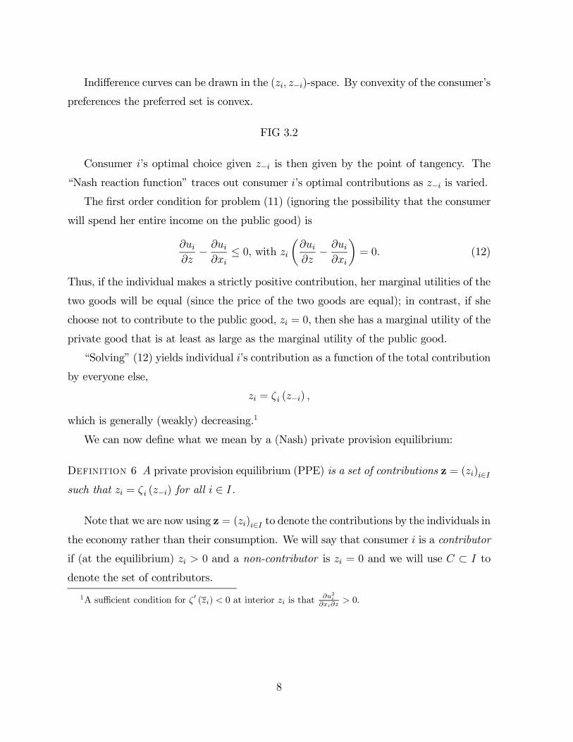
Indifference curves can be drawn in the (zi, z−i)-space. By convexity of the consumer’s

preferences the preferred set is convex.

FIG 3.2

Consumer i’s optimal choice given z−i is then given by the point of tangency. The

“Nash reaction function” traces out consumer i’s optimal contributions as z−i is varied.

The first order condition for problem (11) (ignoring the possibility that the consumer

will spend her entire income on the public good) is

∂ui∂z− ∂ui

∂xi≤ 0, with zi

µ∂ui∂z− ∂ui

∂xi

¶= 0. (12)

Thus, if the individual makes a strictly positive contribution, her marginal utilities of the

two goods will be equal (since the price of the two goods are equal); in contrast, if she

choose not to contribute to the public good, zi = 0, then she has a marginal utility of the

private good that is at least as large as the marginal utility of the public good.

“Solving” (12) yields individual i’s contribution as a function of the total contribution

by everyone else,

zi = ζ i (z−i) ,

which is generally (weakly) decreasing.1

We can now define what we mean by a (Nash) private provision equilibrium:

Definition 6 A private provision equilibrium (PPE) is a set of contributions z = (zi)i∈Isuch that zi = ζ i (z−i) for all i ∈ I.

Note that we are now using z = (zi)i∈I to denote the contributions by the individuals in

the economy rather than their consumption. We will say that consumer i is a contributor

if (at the equilibrium) zi > 0 and a non-contributor is zi = 0 and we will use C ⊂ I todenote the set of contributors.

1A sufficient condition for ζ 0 (zi) < 0 at interior zi is that∂u2i∂xi∂z

> 0.

8

4.1 Existence*

The first question is if a private provision equilibrium generally exists. The answer is yes.

Proposition 1 A private provision equilibrium exists.

Proof. Let n = 2 (the generalization to n ≥ 2 is obvious) and let z = (z1, z2) and letHi = [0, Ri] (the set of possible contributions for i), i = 1, 2. Note that ζ i : Hj → Hi,

j 6= i.ζ i (·) here is the Nash “reaction function”, which tells us what is i’s optimal choice

for every possible choice for j. ζ i (·) is a continuous function by the fact that it is derivedfrom a well-behaved optimization problem. In that problem, convexity of consumer i’s

preferences implies that i’s utility maximisation problem has a unique solution — hence

ζ i (·) is single-valued; moreover, continuity of the utility function ui (·) (in xi, zi and zj)implies that ζ i (·) is a continuous function.The vector z∗ ∈ H1 ×H2 is a PPE if

z∗1 = ζ1 (z∗2) , and z

∗2 = ζ2 (z

∗1) .

Define bζ1 (z) = ζ1 (z2) and bζ2 (z) = ζ2 (z1) .

(This simply extends the definition of ζ1 (·) to have the own contribution as an “irrelevant”argument; this is done so as to ensure that each function becomes a function of the entire

vector of contributions.) Note that bζ i : H1 ×H2 → Hi, i = 1, 2. Then define the vector

valued function bζ (z) = ³bζ1 (z) ,bζ2 (z)´ .The vector valued function bζ (·) maps the set H1×H2 into itself and is continuous. SinceH1 × H2 is a nonempty, compact, convex subset of R2, by Brouwer’s theorem bζ has afixed-point z∗, which, by construction constitutes a PPE.

In the case of two consumers there would be a faster route: simply construct the

composite function ζ1 ◦ ζ2 : H1 → H1; this function is continuous since ζ1 and ζ2 are

both continuous. Thus it has a fixed point which identifies a PPE. However, the above

version makes it easier to see how an extension to n ≥ 2 would work. One can also showthat normality of both the private and the public good implies that the PPE is unique.

9

4.2 Inefficiency

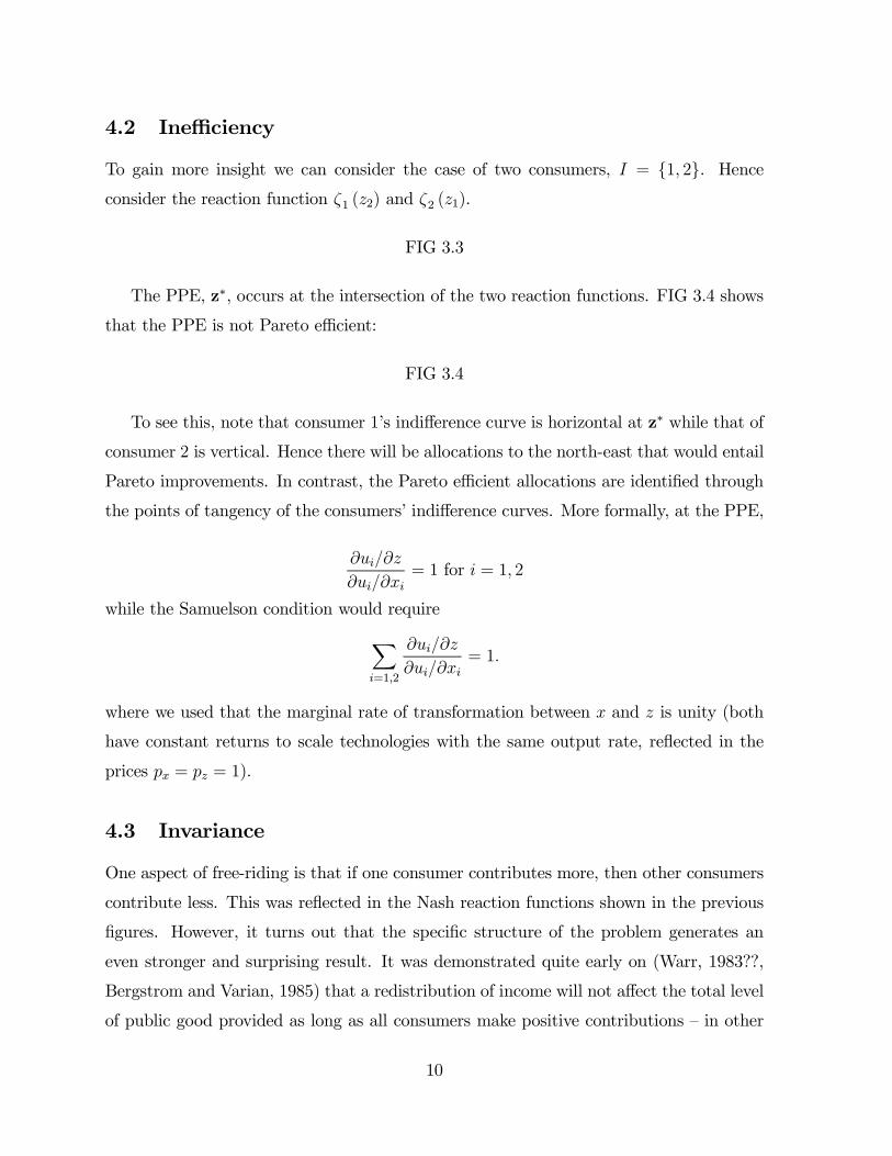
To gain more insight we can consider the case of two consumers, I = {1, 2}. Henceconsider the reaction function ζ1 (z2) and ζ2 (z1).

FIG 3.3

The PPE, z∗, occurs at the intersection of the two reaction functions. FIG 3.4 shows

that the PPE is not Pareto efficient:

FIG 3.4

To see this, note that consumer 1’s indifference curve is horizontal at z∗ while that of

consumer 2 is vertical. Hence there will be allocations to the north-east that would entail

Pareto improvements. In contrast, the Pareto efficient allocations are identified through

the points of tangency of the consumers’ indifference curves. More formally, at the PPE,

∂ui/∂z

∂ui/∂xi= 1 for i = 1, 2

while the Samuelson condition would requireXi=1,2

∂ui/∂z

∂ui/∂xi= 1.

where we used that the marginal rate of transformation between x and z is unity (both

have constant returns to scale technologies with the same output rate, reflected in the

prices px = pz = 1).

4.3 Invariance

One aspect of free-riding is that if one consumer contributes more, then other consumers

contribute less. This was reflected in the Nash reaction functions shown in the previous

figures. However, it turns out that the specific structure of the problem generates an

even stronger and surprising result. It was demonstrated quite early on (Warr, 1983??,

Bergstrom and Varian, 1985) that a redistribution of income will not affect the total level

of public good provided as long as all consumers make positive contributions — in other

10

words — the overall equilibrium contribution would be invariant to income redistribu-

tion. However, the assumption that all individual are making positive contributions is

rather restrictive — in many cases we would expect a large number of individuals to not

contribution at all. The question is if then if the total level of contributions will still be

invariant to income redistributions, or, if not, whether income redistribution will increase

or decrease the total equilibrium level of the public good.

Hence the question we ask here is: How will a redistribution of income affect the

total voluntary provision? To simplify the analysis we will make the assumption that all

individual have identical preferences.

Assumption 1 All consumers have identical preferences: ui = u for all i ∈ I.

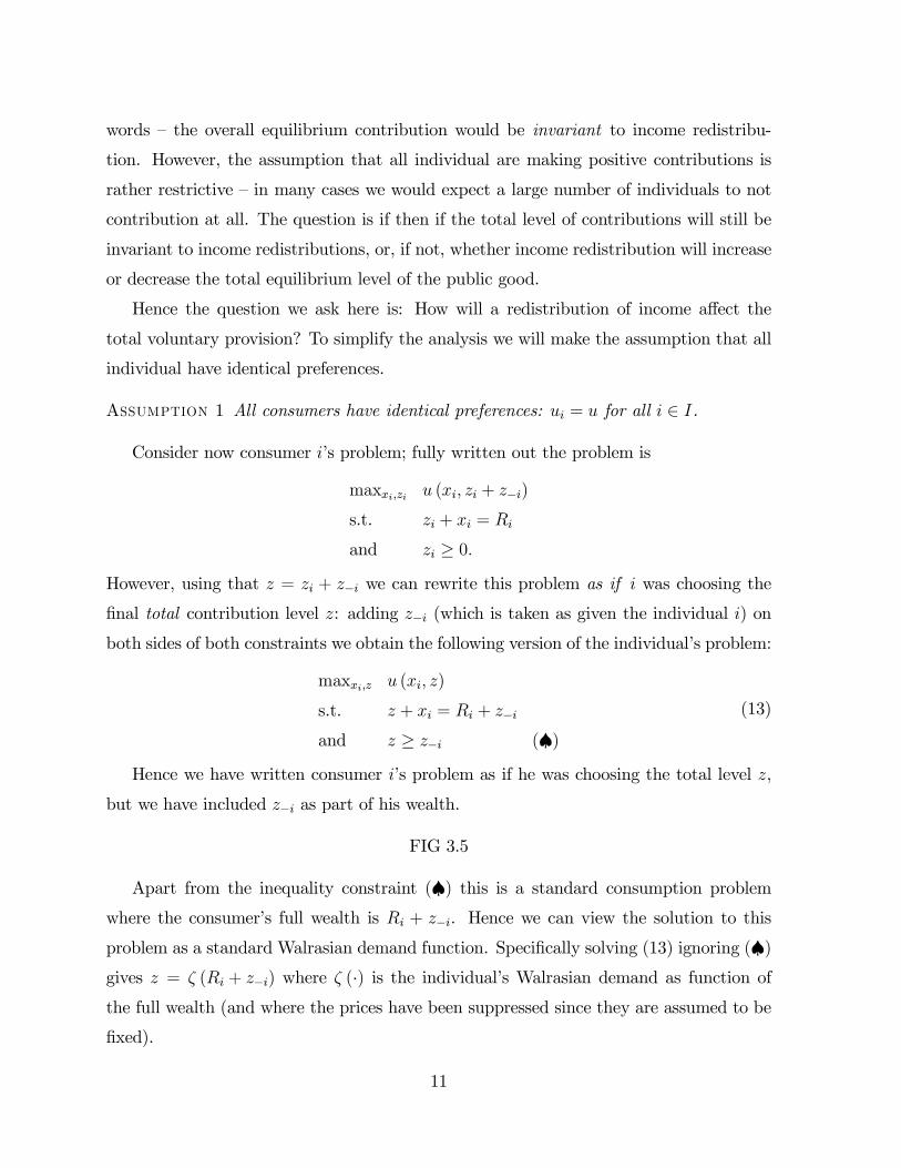
Consider now consumer i’s problem; fully written out the problem is

maxxi,zi u (xi, zi + z−i)

s.t. zi + xi = Ri

and zi ≥ 0.However, using that z = zi + z−i we can rewrite this problem as if i was choosing the

final total contribution level z: adding z−i (which is taken as given the individual i) on

both sides of both constraints we obtain the following version of the individual’s problem:

maxxi,z u (xi, z)

s.t. z + xi = Ri + z−i

and z ≥ z−i (♠)(13)

Hence we have written consumer i’s problem as if he was choosing the total level z,

but we have included z−i as part of his wealth.

FIG 3.5

Apart from the inequality constraint (♠) this is a standard consumption problemwhere the consumer’s full wealth is Ri + z−i. Hence we can view the solution to this

problem as a standard Walrasian demand function. Specifically solving (13) ignoring (♠)gives z = ζ (Ri + z−i) where ζ (·) is the individual’s Walrasian demand as function ofthe full wealth (and where the prices have been suppressed since they are assumed to be

fixed).

11

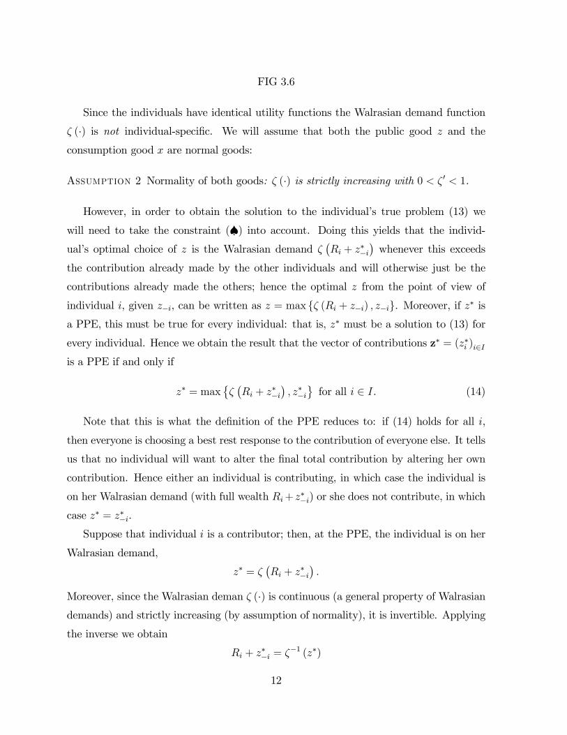
FIG 3.6

Since the individuals have identical utility functions the Walrasian demand function

ζ (·) is not individual-specific. We will assume that both the public good z and theconsumption good x are normal goods:

Assumption 2 Normality of both goods: ζ (·) is strictly increasing with 0 < ζ 0 < 1.

However, in order to obtain the solution to the individual’s true problem (13) we

will need to take the constraint (♠) into account. Doing this yields that the individ-ual’s optimal choice of z is the Walrasian demand ζ

¡Ri + z

∗−i¢whenever this exceeds

the contribution already made by the other individuals and will otherwise just be the

contributions already made the others; hence the optimal z from the point of view of

individual i, given z−i, can be written as z = max {ζ (Ri + z−i) , z−i}. Moreover, if z∗ isa PPE, this must be true for every individual: that is, z∗ must be a solution to (13) for

every individual. Hence we obtain the result that the vector of contributions z∗ = (z∗i )i∈Iis a PPE if and only if

z∗ = max©ζ¡Ri + z

∗−i¢, z∗−i

ªfor all i ∈ I. (14)

Note that this is what the definition of the PPE reduces to: if (14) holds for all i,

then everyone is choosing a best rest response to the contribution of everyone else. It tells

us that no individual will want to alter the final total contribution by altering her own

contribution. Hence either an individual is contributing, in which case the individual is

on her Walrasian demand (with full wealth Ri+ z∗−i) or she does not contribute, in which

case z∗ = z∗−i.

Suppose that individual i is a contributor; then, at the PPE, the individual is on her

Walrasian demand,

z∗ = ζ¡Ri + z

∗−i¢.

Moreover, since the Walrasian deman ζ (·) is continuous (a general property of Walrasiandemands) and strictly increasing (by assumption of normality), it is invertible. Applying

the inverse we obtain

Ri + z∗−i = ζ−1 (z∗)

12

To interpret this, note that the inverse of the Walrasian demand, ζ−1 (z∗), gives the full

wealth that at which the consumer demands z∗; the answer here is it must be Ri + z∗−i.

Now add the own contribution z∗i on each side and use that z∗i + z

∗−i = z

∗; rearranging

give the following expression for the own contribution

z∗i = Ri −£ζ−1 (z∗)− z∗¤ .

This is an intriguing equation: to see this note that the term in brackets is not particular

to individual i. Hence we see that an increase in the individual’s own income Ri increases

her contribution z∗i one-for-one. To make it even more transparent we can denote the

term in the bracket by R∗ = ζ−1 (z∗) − z∗. It is then clear that R∗ denotes the incomelevel of a consumer who “just” contributes at the equilibrium.

Ri < R∗ ⇒ z∗i = 0 (15)

In contrast, any consumer with income above R∗ contributes any income above R∗

Ri ≥ R∗ ⇒ z∗i = Ri −R∗ (16)

FIG 3.7

So summarize:

Lemma 2 If z∗ is a PPE, there exists a critical income level R∗ = ζ−1 (z∗)−z∗ such thatthat all consumers with Ri ≤ R∗ contribute nothing, while any consumer with Ri > R∗contributes z∗i = Ri −R∗.

This result is even more remarkable than it first appears. To see this, consider two

consumers i and j who are both contributing, Ri, Rj > R∗ and suppose that Ri > Rj

(say). Hence they have the same preferences but individual i is richer than individual

j. Consider then the consumption enjoyed by these to individuals. Consider first the

consumption of the private good; from the individual’s budget constraint and using that,

for any contributing individual z∗i = Ri −R∗, it follows that

x∗i = Ri − z∗i = Ri − (Ri −R∗) = R∗. (17)

13

Hence any individual who makes a positive contribution at the PPE will consume x∗i = R∗

units of the private good. Thus our two contributing individuals will enjoy the same level

of the private good. Moreover, since the public good is public they will also enjoy the

same level z∗ of that good. Hence any two contributing individuals will enjoy exactly the

same consumption of both goods; in particular, even though individual i is richer than

individual j, they both enjoy the same equilibrium utility!

This insight should lead us to suspect that it would have no impact on the outcome

if we were to take £1 from individual i and give it to individual j (as long as they are

still both contributing). Indeed, note that we can write the total contribution as

z∗ =Xi∈Iz∗i =

Xi∈C∗

(Ri −R∗) , (18)

where C∗ is the same of individuals who contribute in the PPE. Hence the total contri-

bution is exactly equal to the total amount of income, in excess of R∗, in the group of

contributing individuals. Hence, indeed, if i and j are both contributing in the PPE, then

transferring £1 from one to the other will have no effect on z∗ (nor on the consumptions

of the private good and hence neither on the equilibrium utilities). Similarly, from (18)

redistributing income within the group of non-contributers will have no impact on z∗. In

this case, however, the redistribution will translate one-for-one into changes in private

consumption.

Hence we have the following remarkable result:

Proposition 2 Invariance to income redistributions. Let z∗ be the total contribution of

a public good in a PPE. Then

• Any redistribution of income within the set of contributors will leave z∗ unchanged

• Any redistribution of income within the set of non-contributors will leave z∗ un-changed.

Both these results consider redistribution of income within the groups of contributers

and non-contributers respectively. It can also be shown that:

• A redistribution of income from a contributor to a non-contributor reduces z∗.

14

Example: Intra-Household Redistribution

One intriguing application of this result in the context of public policy is in the context

of intra-household allocations. Suppose e.g. that we are concerned about the equality

between genders and that we want to improve the well-being of wives relative to their

husbands. In general we believe that there are many goods that are effectively “public”

within households, e.g. housing costs, expenditures on children, etc. Suppose then that

are contemplating changing the payment of e.g. child benefit so that it is paid out to

the main carer (most often the female) rather than to the main earner (most often the

male). If the intra-household allocation is one where there is voluntary contributions

by the two spouses to (at least one) household public good, then the redistribution of

income will have no effect on the allocation of consumption within the household — it will

be neutralized by a corresponding change in contributions to the household public good

by the two spouses (Browning, Chiappori, Lechene, 2005??).

4.4 Large Economies*

A feature of the private provision equilibrium is that the individuals are free-riding on

the contributions of other individuals, and some individuals may even choose not to

contribute. Will this be a bigger problem in large economies? Indeed that would seem

most reasonable — as the economy grows, since the public good is non-rivalrous, if no one

changed his or her behavior (in terms of contributions) the total public good provision

would increase. But if the total public good provision increases, then we would expect a

consumer to less willing to make contributions. One way to formalize this is to consider

what happens to the set of contributors as we replicate an economy. What we will see is

that replicating an economy will lead to an equilibrium where a smaller fraction of the

population contributes (Andreoni, 1988).

Hence the question that we considering here is the following: What happens as an

economy grows, in particular, will “free-riding” increase?

To answer this question consider an initial economy described by a set of consumers

I = {1, ..., n} with identical preferences u (xi, z) but with heterogenous incomes (Ri)i∈I .Refer to this as the initial economy, denote E0. From our previous analysis we have that

15

the PPE has the following features. There exists a critical income level R∗0 such that, for

all i ∈ I, the contribution of individual i is max {0, Ri −R∗0} whereby the total privateprovision in E0 is thus z∗0 =

Pi∈I max {0, Ri −R∗0}. Moreover,

R∗0 = ζ−1 (z∗0)− z∗0 . (19)

Note that there is a positive relationship between z∗ and R∗.

Lemma 3 ζ−1 (z∗)− z∗ is a strictly increasing function of z∗.

Proof. Differentiating yields

d¡ζ−1 (z∗)− z∗¢

dz∗=dζ−1 (z∗)dz

− 1 = 1

ζ 0− 1.

Since 0 < ζ 0 < 1 (normality), 1 < 1/ζ 0 <∞ whereby φ0 (z) ∈ (0,∞).Now “replicate” the economy one; for every initial consumer i ∈ I there is now

an “identical twin”. Let E1 to denote “once replicated economy” with consumers 2I.Repeating the steps for the initial economy, in E1 there is a PPE with a critical incomelevel R∗1 such that the contribution of individual i is max {0, Ri −R∗1} and the aggregatecontribution will be z∗1 =

Pi∈I max {0, Ri −R∗1}.

The key result now it that the critical income R∗ will have increased when we go to

the larger economy. Formally:

Proposition 3 The critical income is larger in the replicated economy, R∗1 > R∗0.

Proof. Make the contradicting hypothesis, i.e. suppose that R∗1 ≤ R∗0. Then it immedi-ately follows that

z∗1 ≥ 2z∗0 > z∗0 ,

(where z∗1 = 2z∗0 if R

∗1 = R

∗0). But then, since φ (.) is increasing (Lemma 3)

R∗1 = ζ−1 (z∗1)− z∗1 > ζ−1 (z∗0)− z∗0 = R∗0,

a contradiction.

Since the distribution of income is the same in E1 as in E0 it follows that the fraction ofindividuals who are making positive contributions will have gone down. A slightly more

16

difficult result to demonstrate is that, if we keep replicating the economy, at some point,

only the richest consumers will contribute. Also when we keep replicating the economy

total donations will converge to a finite positive number as the economy grows, but each

consumer will be contributing less and less.

4.5 Empirical and Experimental Evidence on Private Provision

of Public Goods

• Next time... Andreoni (1993, 1995), Maxwell and Ames (1981), Kingsma (1989),Payne (1998) etc.

5 Voting over the Provision of Public Goods

So far we have seen that a private provision equilibrium will lead to underprovision of a

public good. Indeed, this problem is often taken as a justification for public intervention.

This requires collective action and thus some mechanism for collective decision making,

typically voting. Hence we would like to know whether a democratic voting mechanism

will lead to an efficient level of the public good being provided. There are many political

models available which intend to capture different aspects of political processes. However,

we will stick to the most basic model of a political process — we will consider a simple

majority rule model. Hence the question we will be asking here is: Will voting lead to

an efficient level of public good provision?

Before we can provide an answer to this question we will first need to consider how the

public good will be financed. In particular, when voting over the level of the public good,

there must also exist a rule for how the public good is to be financed — a cost-sharing

rule. The cost-sharing rule will have an important role to play in shaping the individuals

preferences over the level of the public good.

We will give two examples. The first example that we will consider is one where

there the individuals in the economy have identical preferences but different incomes and

where the public good is finance through linear taxation. The second example will have

individuals with heterogenous preferences, equal income and equal cost-shares.

17

5.1 Example 1: Implicit Redistribution

As before suppose there is a public good z and a private good x each with unit prices. The

individuals are assumed to have identical preferences. To make to problem particularly

transparent we will assume that preferences are quasi-linear,

u (xi, z) = αxi +H (z) , (20)

where H (·) is twice continously differentiable, strictly increasing and strictly concave.Incomes, Ri, differ across the consumers.

Efficiency

To establish a benchmark we consider first the Pareto efficient level of the public good

in this particular setup. Hence we make use of the Samuelson rule that states that the

sum of the individual’s marginal rates of substitution should equal the marginal rate of

transformation. Note that the marginal rate of substitution takes a particularly simple

form due to the assumption of quasi-linear preferences; in particular:

∂ui/∂z

∂ui/∂xi=H 0 (z)α

for all i ∈ I

Thus, from the Samuelson rule, we have that Pareto efficiency requiresXi∈I

∂ui/∂z

∂ui/∂xi= 1⇐⇒ H 0 (z) =

α

n.

where we used that the marginal rate of transformation between z and x is unity.

Since the marginal utility H 0 (·) is continuous and strictly decreasing it is invertible:let Ψ (·) be the inverse of H 0 (·), i.e. Ψ = (H 0)−1 Since H 0 (·) is strictly decreasing, so isΨ (·). The Pareto efficient level of the public good, which we will denote here by z∗, isuniquely determined by

z∗ = Ψ³αn

´. (21)

Why is the Pareto efficient level of the public good “unique” in the sense that it is

independent of the distribution of utilities? This follows from the quasi-linearity of utility

in income: to achieve a different utility distribution, only consumption of the private good

should be shifted. The linearity implies that utility is effectively transferable. From (21)

18

we also see that the level of the public good should be smaller the stronger are the

preferences for the private good as measured by α and the fewer individuals there are in

the economy.

Since the Pareto efficient level of the public good, z∗, is unique in this case we have a

good benchmark case. Hence we want to know whether voting over the public provision

of z will lead to a level of the public good that is efficient?

Taxation

Suppose that z is finance by a linear income tax with tax rate τ . Consumption of the

private good is what remains of the individual’s income after the tax has been collected:

xi = (1− τ)Ri for all i ∈ I. (22)

The government spends the tax revenues on the public good; hence

z =Xi∈I

τRi ⇔ z = τnR

where R is the average income.

Using the government’s budget constraint to eliminating τ from (22) private consump-

tion will be

xi =

µ1− z

nR

¶Ri for all i ∈ I. (23)

Then, using (23) to replace xi in consumer i’s preferences (20), gives consumer i’s

induced preferences over z, denoted vi,

vi (z) = α

µ1− z

nR

¶Ri +H (z) .

The “preferences” vi (z) describes the utility obtained by individual i when the level

of public provision is z. Hence vi (z) describes individual i’s preferences over policy. Note

that vi (·) is strictly concave in z; the first term is linear in z while the second is strictly

concave. Using the government’s budget balance condition, we have thus managed to

reduce the problem to a single-dimensional policy problem — determining z — and vi (z)

states consumer i’s preferences over different levels of z.

We will be looking for a policy that is favoured by a majority over any other alterna-

tive.

19

Definition 7 A Condorcet winner is a policy that beats any other feasible policy in a

pairwise comparison.

The first thing to figure out is what policy each consumer will like the most, i.e. her

“ideal policy” or “bliss point”. This is the policy that maximizes vi (z). Since vi (z) is

strictly concave individual’s ideal policy, which we will denote zi, is unique. In particular,

zi is characterized bydvidz

= −αRi

nR+H 0 ¡zi¢ = 0.

The next insight is that, since vi (·) is concave in z, consumer i’s preferences over thelevel of public provision are single-peaked.

Definition 8 Policy preferences of consumer i are single peaked if the following state-

ment is trueIf z00 ≤ z0 ≤ zi, or, if z00 ≥ z0 ≥ zi

then vi (z00) ≤ vi (z0) .

FIG 3.8

Using that Ψ = (H 0)−1, we can “solve” for zi,

zi = Ψ

µαRi

nR

¶. (24)

A well-known fact is that, if all voter have single peaked preferences, then a Condorcet

winner exists.

Theorem 4 The Median Voter Theorem. If all voters have single-peaked preferences

(over a given ordering of policy alternatives), a Condorcet winner exists and coincides

with the median-ranked bliss-point.

This leaves the question: who has the median-ranked bliss-point? The answer is

straightforward: it will be the individual with the median income. To see this, note that

from (24) we see that the individual’s ideal policy zi is strictly decreasing in the individual

income Ri. Hence if we rank the individuals in terms of their bliss points we obtain the

reverse of the income ranking; this implies that the individual who is in “the middle” in

terms of the income ranking is also in the middle in terms of the ranking of bliss points!

20

The reason why the bliss-point is decreasing in income is that the public good supply

effectively redistributes income from high-income consumers to low-income consumers.

Everyone obtains the same level of the public good (obviously), however, the high-income

consumers pay more taxes to finance it. Hence they will oppose high levels of the public

good. At the other extreme, a consumer with very little income effectively gets the public

good for free.

Let Rm be the income of the median-income consumer. By the Median Voter Theorem

we then know that the Condorcet winner is the bliss point for the individual with income

Rm. Hence the winning policy is the one where the level of public provision is

zm = Ψ

µαRm

nR

¶. (25)

Most realistic income distributions are skewed so that the median is lower than the

mean, Rm < R. Hence suppose that this is the case. We can then compare the winning

policy to the efficient level of the public good.

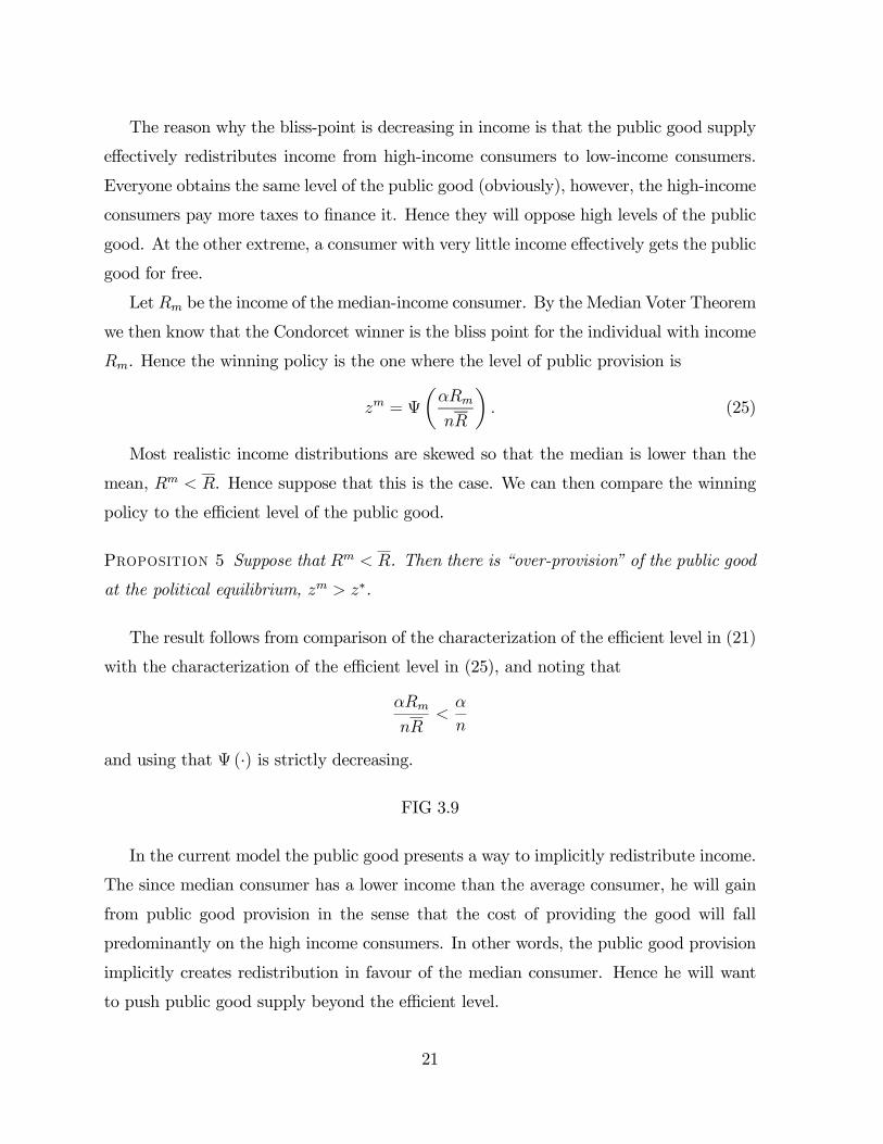
Proposition 5 Suppose that Rm < R. Then there is “over-provision” of the public good

at the political equilibrium, zm > z∗.

The result follows from comparison of the characterization of the efficient level in (21)

with the characterization of the efficient level in (25), and noting that

αRm

nR<

α

n

and using that Ψ (·) is strictly decreasing.

FIG 3.9

In the current model the public good presents a way to implicitly redistribute income.

The since median consumer has a lower income than the average consumer, he will gain

from public good provision in the sense that the cost of providing the good will fall

predominantly on the high income consumers. In other words, the public good provision

implicitly creates redistribution in favour of the median consumer. Hence he will want

to push public good supply beyond the efficient level.

21

5.2 Example 2: Heterogenous Preferences

In the previous example, the cost-shares were determined by the assumption that the

public good was financed through proportional taxation of incomes. The proportional

taxation implied that consumers with below average incomes implicitly gained from public

good provision — effectively if there were n consumers, then any consumer with below

average income will be paying less then 1/n of the total cost. With the majority of

individuals having less than average income the equilibrium provision ended up being

“too high”.

That voting does not generate a Pareto optimal level of a public good a very general

phenomenon. To see this, let’s consider a second example. Whereas in the previous case

we assumed that everyone had identical preferences, but that the implicit cost-shares

differed across the consumers, we will now go in the opposite direction and assume that

the cost-shares are identical, but that preferences are not.

Assume again n consumers i ∈ I = {1, ..., n}. The individuals have the same incomes,Ri = R for all i ∈ I and we assume that there is an agreement that whatever level ofz will be provided, the cost will be shared equally: if z is agreed, then consumer i must

pay 1/n of the cost, i.e. z/n.

Suppose however that tastes differ; consumer i’s utility is

u (xi, z) = xi + βiH (z) , (26)

where βi > 0 measures the strength of individual i’s preferences for the public good and

where H (·) twice continously differentiable, strictly increasing and strictly concave.

Efficiency

As a benchmark, let us first characterize again the Pareto efficient level of the public good

using the Samuelson rule. Note that the marginal rate of substitution for individual i is

∂ui/∂z

∂ui/∂xi=

βiH0 (z)1

for all i ∈ I.

Thus Pareto efficiency requiresXi∈I

βiH0 (z∗) = 1⇔ H 0 (z∗)nβ = 1

22

where β is the average βi. Letting Ψ (·) be the inverse of H 0 (·) and solving for z∗ we have

z∗ = Ψ

µ1

nβ

¶(27)

which is unique since Ψ (·) is strictly decreasing.

Policy Preferences

As in the previous example we should try to determine the individuals’ preferences over

the level of public provision. Note that if the level z is provided, consumer i must pay

z/n. Hence her consumption of the private good will be

xi = R− zn. (28)

Replacing xi in the preferences (26) we obtain the induced policy preferences

vi (z) = R− zn+ βiH (z) .

Consumer i’s bliss-point, denoted zi, maximizes vi (z) and thus satisfies

v0i¡zi¢= −1

n+ βiH

0 ¡zi¢ = 0.Solving for zi we have

zi = Ψ

µ1

nβi

¶. (29)

Noting that the policy preferences vi (·) are strictly concave in z we conclude thatall consumers have single-peaked preferences. Then, by the Median Voter Theorem, the

median ranked bliss-point is the Condorcet winner. In this case there is heterogeneity

among the voters in terms of the strength of their preferences for the public good. In

particular, it individuals with stronger preferences for the public good will have larger

bliss points: using that Ψ (·) is a strictly decreasing function it is easy to see that βi > βj

implies that zi > zk. Hence the individual with the median strength of preferences for

the public good will also be the individual with the median bliss point.

Hence let βm be the preference-parameter of the consumer with the median strength

preferences for the public good. Then the unique Condorcet winner is

zm = Ψ

µ1

nβm

¶. (30)

23

Suppose e.g. that this is a public good that is very much desired by a relatively small

group; most people are not that bothered about the public good. In that case we would

expect the average to exceed the median. Indeed comparing the characterization of the

winning policy (30) to the efficient policy (27) we obtain the following result:

Proposition 6 Suppose that β > βm; then there is “under-provision” at the political

equilibrium zm < z∗.

In this case we have the “tyranny of the majority”: some group would value the public

good a lot. However, the median consumer does not. The median voter is pivotal, and

hence there will be under-provision at the political equilibrium.

6 Club Goods*

The basic public good model is interesting; however, are there really that many cases

where the pure public good model fits as a description of the real world? In fact many

public goods can be viewed as being

• congested (i.e. there is some rivalry)

• locally provided (in the sense of being enjoyed by a subset of the population).

These features makes the story quite a lot more intriguing. Suppose that we have a

good from which people can be excluded. And suppose also that there is some congestion

- e.g. a park. How many people should then share a common public good.

Back in the 1960s James Buchanan (??) put forward the idea of “club good” — a good

that is enjoyed by a number of consumer, but which is not available to outsiders (see

Cornes and Sandler (1996) for an introduction to club goods). So suppose we there is

a public good which is congested in the sense that consumer i’s benefit from it depends

negatively on the number of people also using it. What is then the optimal “club size”?

On the one hand, the more people are using the public good, the smaller are the benefit

to each consumer; but on the other hand, the cost of the public good is spread over a

larger number of individuals.

24

Consider a public good with congestion. Since the public good is crowdable, there

will be an incentive for groups of people to come together to enjoy the good, and to

exclude others. In particular, when a public good is congested, the population may be

partitioned into “clubs”, with each club consuming the locally supplied public good.

Definition 9 A public good is congested if the benefit to a consumer from consuming

it depends negatively on the number of consumers consuming the same good.

To formalize this let z be a public good and x be a private good, each with unit prices.

Let m be the number of consumers using z and let α (·) be a strictly increasing functionwith α (1) = 1. Then define bz = z

α (m)

as the “effective” services of the public good z to a consumer when a total of m consumer

is using the same good.

For simplicity assume identical consumers with preferences u (x, bz) and income R.Note that the individuals derive utility from the “effective” services of the public good

rather than from the level of the public good.

In this setting it is natural to consider the optimal “club size”: how many consumer’s

should be sharing the same public good. Hence we want to know if there is an optimal

“club size” m. To check this we must first determine — for any given club size m — the

optimal amount of z.

Assuming equal cost-sharing, if the amount z is provided, the cost to consumer i is

1/m. Thus, consumption of the private good is (recall that all consumers are identical

here)

x = R− z

m.

The utility of the representative consumer is then

u

µR − z

m,z

α (m)

¶. (31)

Maximizing u with respect to z yields the first order condition

−∂u

∂x

1

m+

∂u

∂bz 1

α (m)= 0,

25

or, by rearranging,

m∂u/∂bz∂u/∂x

= α (m) . (32)

This modified Samuelson rule states that the sum of the marginal willingness to pay for

the effective public good bz (i.e. the left hand side) should equal α (m).Thus the sum of the marginal willingness to pay for the effective public good should

equal α (m). Why α (m) and not unity? This is because — givenm — giving up one unit of

x will increase z by one unit; however, that will only increase the effective public good by

dbz = 1/α (m). Hence the congestion effectively increases the marginal cost of generatingeffective units of the public good.

Consider now the optimal club-size? First, why will there be an optimal club size?

The reason why there will be an optimal club-size is that increasing m has two effects.

One the one hand it reduces the cost to each consumer for any given supply of the public

good z; but on the other hand, it reduces the benefit to a consumer from any given

amount z since it adds to the congestion. Hence, e.g. if there were no congestion, the

optimal club size would be the whole population. If there is congestion it may be optimal

to partition the population into smaller groups (the clubs) enjoying their own public

goods.

Maximize utility in (31) with respect to m. The first order condition is

∂u

∂x

z

m2− ∂u

∂bz z

(α (m))2α0 (m) = 0

which, after using the modified Samuelson rule, reduces to

1 =α0 (m)mα (m)

≡ εαm,

where εαm is the elasticity of α (·) with respect to m.

Proposition 7 The optimal club size, m∗, satisfies εαm = 1.

What is the logic behind the result that the optimal club size is characterized by the

elasticity of α (·) with respect to m being equal to unity? The answer is that it minimizes

the cost of the effective public good. To see this note that the marginal cost of the

“effective” public good bz in terms the private good x isα (m)

m.

26

To see why, note that in order to obtain one unit of “effective” public good bz, α (m) unitsof the underlying public good z are required. But obtaining one unit of z requires giving

up 1/m units of private consumption. Hence to obtain one unit of bz, α (m) /m units of

private consumption need to be foregone.

Then note that if choosing m to minimize the marginal cost α (m) /m we obtain

exactly the optimal club size, m∗.

7 Preference Revelation for Public Goods*

So far we have found that voting equilibria tend to be inefficient. The basic reason is

that they are based on pre-assigned cost-shares as illustrated in the two examples above.

Here is one more example.

Consider an economy with a set of individuals (flat mates) i ∈ {1, .., n} who arecontemplating buying a TV. The TV is a discrete public good so z ∈ {0, 1} and costsc pounds. Consumer i’s utility is ui (xi, z) and her initial income is Ri. Consider i’s

maximum-willingness-to-pay for z. If they do not buy the TV individual i will have the

utility ui (Ri, 0). Hence the maximum-willingness-to-pay for the TV will be the amount

ri where the individual obtains the same utility level.

Definition 10 Consumer i’s reservation price for z is implicitly defined through ui (Ri − ri, 1) =ui (Ri, 0).

In this case the public good is discrete so we have to used a discrete analogue of the

Samuelson rule to determine when it is efficient to buy the TV. From the Samuelson rule

we would expect that it will be efficient to buy the TV if the sum of the individuals’

willingness-to-pay is enough to cover the cost. This intuition is indeed correct.

To see this, note that it is efficient to buy the TV if and only if by doing so some

individual can be made better off while no one else is made worse off. The statement

that no one is worse off simply says that no one will be asked to pay more than her

reservation price. Formally, providing the public good will Pareto dominate not providing

the public good if we can find contributions gi to the cost of the public good such that

everyone is better off with the good being provided than with the public good not being

27

provided. Hence there must be some set of contributions, (gi)i∈I such thatP

i∈I gi = c

and ui (Ri − gi, 1) > ui (Ri, 0). But clearly, this will be the case if and only ifP

i ri > c.

Proposition 8 Providing the public good Pareto dominates not providing the good if

and only ifP

i∈I ri > c.

However, the consumers may not know each other’s preferences. So suppose then that

they decide to vote in order to determine whether to provide the good or not. So suppose,

e.g., that they decide to split the cost equally: if the good is provided each consumer would

have to pay c/n. The question is whether the public good will be provided whenever it

is Pareto efficient to do so. The immediate answer is no. This can be proved by way of

example: Suppose e.g. that n = 3, c = 90, r1 = 60, r2 = r3 = 20. Then since

c

n= 30 > 20 = r2 = r3

consumer 2 and consumer 3 will vote against, despite the fact thatP3

i=1 ri = 100 > 90 =

c.

Indeed, the problem seems to be more pronounced when the distribution of reservation

prices is more dispersed. Obviously, if everyone has the same reservation price, then

voting will generate the Pareto optimal decision. Hence voting based on pre-assigned

cost-shares cannot in general be expected to lead to Pareto efficiency. Ideally we would

like the cost-shares to be related to the reservation prices. But the basic problem is that

we may not know the reservation prices — that’s why we are voting in the first place —

to figure out a “good collective decision”. This raises the question if it is possible to

make the individuals reveal how much they value the public good and, if so, can we reach

Pareto optimality? The answers to these questions turn out to be “yes” and “almost”.

7.1 The Groves-Clarke Mechanism

Consider again the case of a discrete public good z ∈ {0, 1} with cost c.2 There is a setof individuals i ∈ I = {1, .., n} with reservation prices (ri)i∈I and incomes (Ri)i∈I . If thegood is provided, then individual i will pay a share of the cost; let si be individual i’s

cost-share of the public good,P

i∈I si = 1.

2The section is based on Varian (1992) [??]

28

Assume quasi-linear utility

ui (xi, z) = xi + ξiz (33)

In this formulation, individuals i reservation price is precisely ξi. Define consumer i’s net

value, vi, for the public good

vi = ui (Ri − sic, 1)− ui (Ri, 0) = (Ri − sic) + ξi −Ri = ξi − sic.

Note that if we sum up the individuals’ net values we obtainXi∈Ivi =

Xi∈I(ξi − sic) =

Xi∈I

ξi − c (34)

sinceP

i∈I si = 1. Since ξi is individual i’s reservation price it is hence efficient to

provide the public good if and only ifP

i∈I vi > 0 (independently of the distribution of

the cost-shares (si)i∈I).

The question is whether there is any way we can find out the net values. Suppose

we simply ask the consumers to report the net values. This will not be such a good

idea, since the consumers may then have a strong incentive to over- or under report their

true net value. Can we design a scheme where the consumers report their net values

truthfully?

Consider the following mechanism:

1. Each consumer reports a net value (a “bid”) bi which may or may not coincide with

her true net value vi.

2. The public good is provided if and only ifP

i∈I bi ≥ 0.

3. Each consumer receives a side transfer equal to the sum of the other bids,P

j 6=i bj

if the public good is provided (negative ifP

j 6=i bj < 0).

Given this scheme, the optimal strategy for a consumer is to report bi = vi (truthful

reporting) independently of how the other consumers choose their bids, bj. To see this

note that individual i’s payoff takes the form

payoff to i =

⎧⎨⎩ vi +P

j 6=i bj if bi +P

j 6=i bj ≥ 00 if bi +

Pj 6=i bj ≥ 0.

29

In words, if the good gets provided, then individual i gets to pay her share and enjoy

the good; this gives the net utility vi. In addition she obtains the side transferP

j 6=i bj

which, using that utility is linear in private consumption, simply adds to her utility.

Given these payoff, what is i’s best choice if bi? There are two cases to consider:

Case 1. Suppose that vi +P

j 6=i bj > 0.

In this case the good will be provided if individual i reports her true net value (or

something higher). Hence if the individual reports bi = vi the public good will be provided

and her payoff to i will be vi+P

j 6=i bj. Note that in this case the consumer will be better

off if the good is provided since, by assumption, vi+P

j 6=i bj > 0. Now ask if the individual

can do better by reporting anything else than bi = vi.

• Can reporting bi > vi increase individual i’s utility?

The answer is no. With any bi > vi the public good will still be provided and the

individual’s payoff will be unaffected.

• Can reporting bi < vi increase i’s utility?

Again the answer is no. Reporting bi < vi will either leave the payoff unaffected or

it will lead to the public good not being provided, which would lower the individual’s

utility.

Hence, if the consumer is better off with the public good being provided, she has

no reason to either over- or under-report her net value. Consider now the opposite case

where the consumer is better off with the public good not being provided.

Case 2. Suppose that vi +P

j 6=i bj < 0.

If the consumer reports truthfully bi = vi the public good is not provided and her

payoff is 0. Now ask if the individual can do better by reporting anything else than bi = vi

• Can reporting bi > vi increase i’s utility?

Again the answer is no. Reporting bi > vi will either leave the payoff unaffected or it

will lead to the public good being provided, which would lower the individual’s utility.

• Can reporting bi < vi increase i’s utility?

30

The answer is again no. With any bi < vi the public good will still not be provided

and the individual’s payoff will be unaffected.

Thus over- or under-reporting vi can never increase consumer i’s utility, no matter

how the other consumers choose their bids. In particular, the other consumers do not

need to report truthfully.3

So why does this mechanism work? It works effectively by making each consumer

facing the social decision — if consumer i is pivotal in the sense that she alters the decision,

then that will affect the net payment to her which equals the net impact of her decision

on the other consumers in the economy. Hence with this mechanism, the public good is

provided if and only if it is Pareto efficient to do so.

So are there any problems with the mechanism? Yes, the problem is that the side

payment do not in general sum to zero — the sum may be either positive or negative.

Hence, if we e.g. think about the mechanism being run by a government, the government

cannot know a priori whether the policy will generate a surplus or a deficit. It is possible

to redesign the mechanism so as to guarantee non-positive transfers (“Clarke taxes”), but

this may lead to “wasted tax revenue” (which is not Pareto optimal). The problem is

deep: in fact there is no way to design a mechanism that induces truthtelling and which

is always budget balanced. However, if the economy is large, then the budget can be

“almost balanced”.45

8 Externalities: An Overview

We now turn to consider externalities. In fact public goods in a very particular form of

externality: When someone voluntarily provides a public good, other people will benefit

from it too. Hence, what follows is a more general analysis of externalities.

3Truthful reporting is hence a “dominant strategy”.4The basic insight is that it is possible to affect the total transfers by introducing a second transfer to

consumer i; as long as it does not depend on consumer i’s reported benefit it will not affect the incentives

to truthfully report the preferences.5The analysis above was for a discrete public good. Can it be applied to a continous public good?

Yes it can. Assuming quasi-linear preferences the net pay off to consumer i is vi (z) = ϕi (z)− siz; theconsumers can be induced to report the function ϕi (·).

31

Our analysis will proceed in several steps. First we will define what we mean by

externalities and introduce some useful distinctions.

Part 1: Defining externalities and highlighting the market failure

It turns out that it is not actually straigthforward to define an externality. And more-

over, allowing all possible effects within a general equilibrium model be very cumbersome;

hence we will be looking at a mini-example with two producers and one consumer. That

example will be sufficient for understanding what is required from a Pareto optimal allo-

cation.

We will then go on to show why the decentralized equilibrium is inefficient; the de-

centralized equilibrium is also an important benchmark case, since several remedies to

externality problems work by corrective mechanisms within the decentralized framework.

One immediate upshot from that analysis is that one can think about the externality

problem as a problem of missing markets. That in turn suggests that the way to “cor-

rect” externalities would be to establish property rights and to establish the relevant

markets. This is an idea that we will come back to a bit later, but before that we will

consider other types of “solutions”.

Part 2: Solutions based on quotas, subsidies, and taxes

The first obvious solution would be to impose quantity constraints: if a firm, say,

generates a negative externality, then it produces too much output. In that case, imposing

a quota should remedy the problem. However, quantity controls are quite demanding in

terms of information requirement. If there is uncertainty, price controls may be more

appropriate

The traditional public finance solution to externalities is to impose taxes; corrective

taxes are commonly known as Pigovian taxes (after Pigou, 1932). We will show how

corrective taxes should be set equal to the marginal social damage.

However, the problem with Pigovian taxes is that they are equally information de-

manding as quantity controls. Both the quota-policy and a corrective tax-policy require

that the regulator knows the extent of the externality. Suppose that that is not the case.

We might then ask if it is sufficient that the parties involved both know the extent of the

externality. Hence we will consider a mechanism that will work when the parties involved

are well-informed about the externality, but where the regulator is not.

32

After going through those “solutions” we will turn to the idea that establishing prop-

erty rights and establishing the relevant markets will solve the problem. This idea goes

back to James Meade (1952); however, what Meade has in mind was the idea of prices

and price-taking agents. But in many cases, there are only a few parties involved, in

which case the idea of price-taking behavior becomes quite unrealistic. But of course,

markets and price-taking behavior is generally not needed. Suppose e.g. that there are

only two parties: a polluting firm and a negatively affected consumer (say). Then if the

consumer was given the right to a clean environment, the two parties could bargain over

the amount of pollution — most likely, the negative effect of a small amount of pollution

on the consumer will be less than value to the firm in terms of increased profits. In that

case, the Pareto optimal pollution level is strictly positive, and if the two parties bargain

efficiently, they will achieve the Pareto optimal pollution level. This has become known

as the Coase theorem (Coase, 1960).

It is questionable whether the Coase theorem is really a fundamental result — indeed,

in many ways it is nothing but a tautology (there is no missing market problem is a

market is established...) However, it is important in that it points out that the only

government intervention that may be necessary is to establish property rights.

Part 3: Establishing property rights

However, there are several cases where we may be less inclined to believe that the

Coasian approach will lead to an efficient allocation. The first such case is when an ex-

ternality has a public good character; in that case exactly the same type of problem that

we noted for privately provided public goods will reappear. If I buy clean air, that will

benefit everyone else, an effect that I will not take properly into account. Hence I will con-

tribute too little. Externalities with a public good character are know as non-depletable

externalities. The case of non-depletable externality generates problem because it requires

multilateral bargaining — there are numerous agents involved.

However, can we even expect the Coase claim to hold in the case of a simple bilateral

externality? Maybe, but then again, maybe not! Another potential problem with the

Coase theorem is that it assumes that the parties bargaining have perfect information

about each others’ costs and benefits. This raises the question what happens when this

is not the case — we will show that bilateral bargaining generally is inefficient when the

33

parties bargaining have private information about their costs and benefits.

9 The Nature of Externalities

Despite the fact that we all sort of know what an externality is, it turns out that it is not

straightforward to define externalities precisely. Consider the following definition:

Definition 11 There is an external effect, or an externality, when some agent’s actions

directly influence either the production possibility set of a producer or the well-being of a

consumer.

Though this sounds straightforward the word “directly” has generated some problems.

In particular, it rules out what has become known as “pecuniary externalities” which are

essentially effects through prices in the markets. (E.g. suppose I start up a firm which

uses a lot of hamp; this brings up the price of hamp, which reduces the profitability

of other firms using the same input. That would be a pecuniary externality — not an

externality defined as above — and indeed, would not cause ineffiencies; at least not in an

economy characterized by competition.)

Definition 12 An externality that is favorable (unfavorable) to the recipient is referred

to as a positive (negative) externality.

Definition 13 An externality is said to be bilateral if there are only two parties involved,

and multilateral if there more parties involved. Multilateral externalities are said to be

depletable when they are “rivalrous” and non-depletable when they are “nonrivalrous”.

By nonrivalrous we mean that the externality has a public good (or public “bad”)

character. This distinction will be important when we talk about the prospect of solving

the externality problem by establishing property rights.

9.1 The Pareto Optimum

We don’t need to use the fully general case with n consumers and m firms in order to

understand how externalities will affect the characterization of a Pareto optimum. Indeed,

34

the fully general case would generate more notation than insights. Hence we will consider

a simplified example with just two firms and one consumer.

Specifically, suppose there are two externalities affecting firm 2: one generated by the

consumer and one generated by firm 1.

FIG 3.10

There are two goods in the economy and the consumer’s preferences are defined over

these two goods, u (x1, x2) . The preferences are assumed to be strictly convex.

Firm 1 produces good 1 using good 2 as input. Denote the input ξ2, and the output

y1. Hence we assume that y1 = f1 (ξ2) where f1 is increasing and concave and represents

firm 1’s technology.

Firm 2 produces good 2 using good 1, but is also affected by the consumer’s consump-

tion of good 1, i.e. x1 and the output generated by firm 1 y1. Hence y2 = f2 (ξ1, y1, x1),

where f2 is increasing and concave in ξ1 and represents firm 2’s technology and how

firm two is affected by y1 and x1. The externalities are both assumed to be “negative”:

∂f2/∂y1 < 0 and ∂f2/∂x1 < 0.

The economy has an initial aggregate endowment of the two goods ω = (ω1,ω2).

Since we only have one consumer in the economy, the Pareto optimum can be found by

maximizing the utility of this one consumer. Hence consider the following problem:

max u (x1, x2)

x1 + ξ1 ≤ ω1 + f1 (ξ2)

x2 + ξ2 ≤ ω2 + f2 (ξ1, f1 (ξ2) , x1)

(35)

by choice of (x1, x2, ξ1, ξ2). The first constraint says that the use (in consumption and as

input) of good 1 should not exceed what is available (as endowment and as output) of

that goods. The second constraint makes the same statement for good 2.

If (x∗1, x∗2, ξ

∗1, ξ

∗2) is a solution, then by the Kuhn-Tucker theorem, there exists (λ

∗1,λ

∗2)

such that the partial derivatives of the associated Lagrangian L is zero (at that point);the partial derivatives reduce to

∂u

∂x1− λ∗1 + λ∗2

∂f2∂x1

= 0 (36)

35

∂u

∂x2− λ∗2 = 0 (37)

−λ∗1 + λ∗2∂f2∂ξ1

= 0 (38)

−λ∗2 + λ∗1∂f1∂ξ2

+ λ∗2∂f2∂y1

∂f1∂ξ2

= 0 (39)

What is the interpretation of the multipliers? λ∗h measures the social marginal val-

uation of good h. In particular, the way we have set up the problem, λ∗h measures the

value — in terms of the objective function, i.e. the consumer’s utility — of having one more

unity of good h.

From basic micro theory we know that Pareto efficiency requires that all consumers’

marginal rates of substitution should be the same and, moreover, should be equal to the

firm’s marginal rates of transformation. Translated into the current example, if there

were no externalities, the optimum would have MRS =MRT 1 =MRT 2, i.e.

∂u/∂x1∂u/∂x2

=∂f2∂ξ1

=

µ∂f1∂ξ2

¶−1.

The reason why the latter marginal product has to be inverted is that firm 1 produces

good 1 from good 2 — hence ∂f1/∂ξ2 measures dx1/dx2 not dx2/dx1. How will the

externalities change this characterization of Pareto optimality? Using (37) to manipulate

(36) we obtain∂u/∂x1 + (∂u/∂x2) (∂f2/∂x1)

∂u/∂x2=

λ∗1λ∗2. (40)

Similarly, from (38) we obtain∂f2∂ξ1

=λ∗1λ∗2. (41)

Finally, from (39) we obtain

1− (∂f2/∂y1) (∂f1/∂ξ2)(∂f1/∂ξ2)

=1

∂f1/∂ξ2− ∂f2

∂y1=

λ∗1λ∗2. (42)

The left hand side of (40) can be called the social marginal rate of substitution; it

takes into account the externality caused by consumption of good 1.When the consumer

consumes one more unit of good 1 it directly increases her utility by ∂u/∂x1 but it also

reduces the output of good two by ∂f2/∂x1 which affects the objective function — i.e. the

consumer’s utility — by (∂u/∂x2) (∂f2/∂x1). In contrast, when the consumer consumes

36

one more unit of good two, this only has the direct effect ∂u/∂x2 since this is not causing

any externality.

Firm 2 is not generating any externalities; hence at the optimum, its marginal rate of

transformation should be equal to the relative social marginal values of the two goods,

which is exactly what (41) tells us.

Firm 1’s production on the other hand reduces the production of good 2, its marginal

rate of transformation at the Pareto optimum takes the negative effect into account as

shown in (42). When firm 1 uses one additional unit of good 2, it produces ∂f1/∂ξ2

extra units of good 1. However, by the externality, this reduces the output of good 2 by

(∂f2/∂y1) (∂y1/∂ξ2).

Thus, the first lesson is that, even when there are negative externalities involved,

this does not require total elimination of their sources — only that the external effect are

somehow internalized : it does not require that the consumer does not consume good 1

of that first 1 shuts down its production.

9.2 Inefficiency of the Competitive Equilibrium

We can now readily verify that a competitive equilibrium fails to be Pareto efficient.

Hence suppose that this economy was at a competitive equilibrium with prices p =

(p∗1, p∗2). Of course, at the competitive equilibrium, the consumer sets her marginal rate

of substitution equal to the price ratio; moreover, each firm sets its marginal product

equal to the price ratio. E.g. firm 1 solves the following profit maximization problem,

maxξ2{p1f1 (ξ2)− p2ξ2} .

which generates the first order condition p1/p2 = (∂f1/∂ξ2)−1. Utility- and profit maxi-

mization then implies that, at the decentralized competitive equilibrium,

∂u/∂x1∂u/∂x2

=∂f2∂ξ1

=

µ∂f1∂ξ2

¶−1=p∗1p∗2,

which, as just argued, would fail to be Pareto efficient. Normally we would expect that

too much of good 1 will be produced and consumed.

37

10 Interventions for Externalities

10.1 Quota Policy

The simplest way to arrive at a Pareto optimum is of course for the government to set

quotas specifying that the externality generating activities should be set at their Pareto

optimal levels.

Hence suppose that the government designs a quota policy that imposes the quantity

constraint that x1 ≤ x∗1 and y1 ≤ y∗1. Note that we are relying heavily on the convexityof the preferences, and on concavity of the production function for this policy to work.

Given the quotas (x∗1, y∗1) the Pareto optimal allocation is indeed an equilibrium allocation:

consider prices (p∗1, p∗2) that are proportional to relative social marginal values (λ

∗1,λ

∗2).

We want to verify that, given the quota policy, the prices (p∗1, p∗2) along with the Pareto

optimal quantities constitute a competitive market equilibrium. Firm 2 does not face any

quota on its output and hence maximizes it profits given the prices (p∗1, p∗2) which leads

to∂f2∂ξ1

=p∗1p∗2=

λ∗1λ∗2

(43)

which verifies that (41) is satisfied; the firm will produce the Pareto optimal output level

y∗2.

Consider then firm 1. We know that its profit function is concave. Hence the firm

would like to produce at the level where

1

∂f1/∂ξ2=p∗1p∗2=

λ∗1λ∗2

(44)

However, that would violate the quota policy. Instead it will optimally produce the

maximum amount allowed by the quota. Hence the firm will optimally produce the

Pareto optimal amount y∗1.

FIG 3.11

Finally, by strong convexity of the preferences, (x∗1, x∗2) is optimal for the consumer as

illustrated by next figure.

FIG 3.12

38

Moreover, since (x∗1, x∗2, y

∗1, y

∗2) is just feasible, we also know that the markets will are

clearing. Hence the quota policy works under the assumption of convexity of the firm’s

production possibility sets and of the individuals’ preferences. However, it should also be

noted that it is a very information-demanding policy. It requires precise information so

that x∗1 and y∗1 can be calculated.

10.2 Corrective Taxes

The traditional public finance solution to externalities is “corrective taxation” or “Pigou-

vian taxation”. Hence, continuing with the previous example, suppose that the govern-

ment can impose commodity taxes. In particular, suppose that the government imposes a

tax t be a tax per unit of x1 purchased and another tax τ be a tax per unit of y1 produced.

Hence the taxes are levied on the externality-generating activities. Since the taxes will

generate tax revenue, that revenue will somehow have to be returned to the economy. We

assume that any collected tax revenue is given to the consumer as lump-sum transfer T .

Consider then the competitive equilibrium with producer prices (p∗1, p∗2). Since there

is a tax on good 1 the consumer price of good 1 will be p∗1. Consider first the consumer.

Facing the prices (p∗1 + t, p∗2) she solves the problem

maxx{u (x1, x2) | (p∗1 + t∗) x1 + p∗2x2 = R∗} , (45)

where

R∗ = (p∗1 + t∗)ω1 + p∗2ω2 + T

∗ + π∗1 + π∗2

is the consumer’s wealth. Note that the consumer owns the initial endowment (which is

valued at the market prices (p∗1 + t, p∗2)), receives the transfer T

∗ and also own the profits

from the firms, denoted π∗1 and π∗2. The lump-sum transfer equals

T ∗ = t∗x∗1 + τ∗y∗1.

Each firm maximizes its profits; hence the profits for firm

π∗1 = maxξ2{(p∗1 − τ∗) f1 (ξ2)− p∗2ξ2} , (46)

where we used that this firm faces a tax of τ ∗ per unit of output. Similarly for firm 2

profits are

π∗2 = maxξ1{p∗2f2 (ξ1, y∗1, x∗1)− p∗1ξ1} . (47)

39

Now suppose that the taxes are set to equal the value of the marginal external effects

(at the Pareto optimum)

t∗ = −p∗2∂f2∂x1

, and τ∗ = −p∗2∂f2∂y1

. (48)

At the competitive equilibrium (45) the consumer chooses to consume where the

marginal rate of substitution is equal to the ratio of consumer prices; hence

∂u/∂x1∂u/∂x2

=p∗1 + t

∗

p∗2; (49)

while profit maximization by firm 1 (46) implies that

(p∗1 − τ∗)p∗2

=

µ∂f1∂ξ2

¶−1, (50)

and profit maximization by firm 2 (47) implies that

∂f2∂ξ1

=p∗1p∗2. (51)

But, using (48), (49) through (51) implies that the ratio of the equilibrium prices satisfy,

p∗1p∗2

=∂u/∂x1 + (∂u/∂x2) (∂f2/∂x1)

∂u/∂x2

=∂f2∂ξ1

=

"µ∂f1∂ξ2

¶−1− ∂f2

∂y1

#;

The equality of the last three terms was precisely the characterization of the Pareto

efficient allocation (x∗1, x∗2, ξ

∗1, ξ

∗2).

6

Proposition 9 Given that the consumer’s preferences and the firms’ production possi-

bility sets are convex, Pigouvian taxes can restore the Pareto optimum.

Convexity here plays very much the same role as it does in the second fundamental

theorem of welfare economics — it ensures that the marginal condition indeed uniquely

characterize the agents’ best choices.7

6When profits accrue to the consumer and she also receives the transfer T ∗ = t∗x∗1 + τ∗f1 (ξ∗2) she

can just afford to buy (x∗1, x∗2).7One should be a bit careful though — given the taxes (t∗, τ∗) there may be other competitive equilibria

— in other words, we might worry about equilibrium multiplicity.

40

FIG 3.13

FIG 3.14

The corrective taxation solution also has the same problem as a quota policy: it

requires detailed information about preferences and technologies.

10.3 A Compensation Mechanism*

Quotas and taxes thus require that the regulator knows the costs and benefits associated

with an externality. This may not always be true; in particular, it is reasonable to think

that the parties involved have a better idea. What we will show is that, if there is

a bilateral externality between two firms which both parties have perfect information

about, then one can design a mechanism that will make the both agree on the correct

Pigouvian tax.8

Consider the same setup as before, only assume that consumption does not generate

any externality. Hence focus on externalities in production (from firm 1 to firm 2):

y1 = f1 (ξ2) and y2 = f2 (ξ1, y1) .

As before, Pareto optimality requires

∂f2∂ξ1

=

µ1

∂f1/∂ξ2− ∂f2

∂y1

¶Suppose that the government doesn’t know the size of the externality but that the

firms both know the size of the externality. A Pigovian tax cannot then immediately be

set — the government does not have the information required to do so. Hence we would

like to know whether the firms can be induced to reveal the size of the externality?

Consider the following mechanism which has two stages:

Stage 1: Each firm j announces a tax level τ j which may or may not coincide with the

Pigovian tax −p2 (∂f2/∂y1).Stage 2: If firm 1 produces y1, it has to pay a tax τ 2y1 while firm 2 receives a compen-

sation τ1y1. In addition, each firm pays a penalty if τ1 6= τ 2, e.g. (τ 1 − τ2)2.

8This section is based on Varian (1992). [Should check original ref...]

41

The precise form of the penalty doesn’t matter as long as it is positive when τ1 6= τ2

and zero when τ 1 = τ 2.

Note that each firm cannot directly affect the tax it pays/compensation it receives by

its own announcement: firm 1’s tax payment is based on the tax announced by firm 2,

and the compensation firm 2 receives is based on the tax that firm 1 announced. This

breaks the link between the own tax announcement and the one payment/compensation;

finally — the penalty implies, as we will see, that both parties will have an incentive to

announce the same tax.

One can then show that it is optimal for each firm to announce the Pigovian tax. To

do this, we will solve for a subgame perfect equilibrium (SPE) using backwards induction.

Note that the game has two stages: first the firms announce tax rates, and then they

choose output levels. We use an SPE to make sure that no equilibria are upheld by

threats that are not credible.

Solving stage 2 given (τ 1, τ2).

After the taxes have been announced, each firm chooses its production; hence firm 1

chooses the level of its input ξ2, and firm 2 chooses the level of its input ξ1. Given prices

p = (p1, p2) and tax announcements (τ 1, τ2), firm 1’s profits are

π1 = (p1 − τ 2) f1 (ξ2)− p2ξ2 − (τ 1 − τ 2)2 , (52)

which are maximized when

(p1 − τ 2)∂f1∂ξ2

= p2. (53)

Note that firm 1’s output will depend on τ2, i.e. y1 (τ2); by concavity of f1, y01 (τ2) < 0.

Intuitively, the smaller is the net-of-tax price for its output, the less firm 1 will produce.

Firm 2’s profits are

π2 = p2f2 (ξ1, y1)− p1ξ1 + τ 2y1 − (τ 1 − τ2)2 , (54)

which are maximized when

p2∂f2∂ξ1

= p1. (55)

Having characterize the output levels, we can now turn to the first stage — the announce-

ment of taxes.

42

Solving stage 1

Consider first firm 1. In order to maximize π1 firm 1 always wants to set

τ 1 = τ 2. (56)

This is immediately clear from (52): firm 1 is affected by its own announcement only

through the penalty function; hence firm 1’s problem reduces to trying to predict what

firm 2 will announce.

So what will firm 2 announce? Intuitively firm 2 has three goals — maximizing the

transfer it receives, maximizing its own operational profits, and minimizing the penalty

for differing announcements. However, it can effectively ignore the last goal since we

know that firm 1 will have the incentive to exactly match firm 2’s announcement!

Since firm 1 has the incentive to match τ 2, firm 2 will set τ2 to maximize the sum of

its own operational profits plus the received transfer. Maximize π2 by choosing τ2,

∂π2∂τ2

=

µp2

∂f2∂y1

+ τ2

¶y01 (τ 2) + 2 (τ1 − τ 2) = 0,

where, in light of (56), the last term vanishes at the SPE.

So what is the trade-off here? Firm 2 can effectively choose firm 1’s output by the tax

is chooses to announce. The condition above implies that at the optimum, firm 1 must

be indifferent to marginal variation in y1. The only time he is indifferent about marginal

variation in y1 is when he is exactly compensated for the externality!

Since y01 (τ2) < 0 firm 2 optimally announces

τ2 = −p2∂f2∂y1

. (57)

Combining (57) with (53) (and rewriting (55)) it follows that, in the SPE,µ∂f1∂ξ2

¶−1− ∂f2

∂y1=

∂f2∂ξ1

=p1p2.

Thus, with prices (p∗1, p∗2) proportional to (λ

∗1,λ

∗2), the Pareto optimum is obtained in

equilibrium.

Proposition 10 The Compensation Mechanism implements the Pareto optimum, and

in the unique subgame-perfect equilibrium of the tax-announcement game, both firms an-

nounce the Pigovian tax τ∗ = −p∗2 (∂f2/∂y1).

43

11 Establishing Property Rights

The Coase theorem is central to understanding the policy implications of externalities;

it is important because it states the conditions under which we can expect the market

to solve the externality problem with minimal intervention. The minimal intervention

consists simply of establishing property rights. E.g. in the case of a firm polluting and

reducing the profits of a second firm, establishing property rights simply involve specifying

whether firm 1 has the right to pollute, or whether firm 2 has the right to a pollution-free

environment.

Once one grasps the idea behind the Coase theorem, one can also perceive some of

its weaknesses. E.g. in the case of two firms where one is polluting the environment for

the second, it is not clear why bargaining should be necessary: anyone who has access to

sufficient funds should be able to buy both firms and make a profit out of it! Another

serious weakness is that it deals badly with multilateral non-depletable externalities (i.e.

public bads) since there will be a free-rider problem.

The Coase theorem was never formally stated, but a generally agreed version might

read as follows.

Theorem 11 The Coase Theorem. If property rights are clearly stated and transaction

costs are zero, bargaining will lead to an efficient outcome no matter how the property

rights are allocated.

11.1 Some Words about Bargaining

In order to investigate the Coase theorem, we will need to use bargaining theory.9 This

is a large literature on bargaining. However, one can quite broadly split the literature up

into two parts.

First there is a “noncooperative bargaining approach” which models bargaining processes

using noncooperative game theory. A commonly used version is the Rubinstein-Stahl

model. In the basic Rubinstein-Stahl model, two parties bargain over how to split a

given amount of money and the process goes as follows. First player 1 offers a split

9See e.g. Mas-Colell, Whinston and Green (1995, Ch. 22).

44

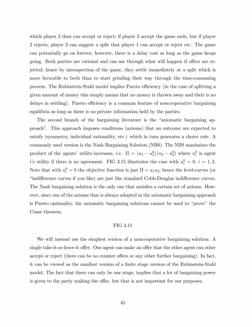
which player 2 then can accept or reject; if player 2 accept the game ends, but if player

2 rejects, player 2 can suggest a split that player 1 can accept or reject etc. The game

can potentially go on forever, however, there is a delay cost as long as the game keeps

going. Both parties are rational and can see through what will happen if offers are re-

jected; hence by introspection of the game, they settle immediately at a split which is

more favorable to both than to start grinding their way through the time-consuming

process. The Rubinstein-Stahl model implies Pareto efficiency (in the case of splitting a

given amount of money this simply means that no money is thrown away and their is no

delays in settling). Pareto efficiency is a common feature of noncooperative bargaining

equilibria as long as there is no private information held by the parties.

The second branch of the bargaining literature is the “axiomatic bargaining ap-

proach”. This approach imposes conditions (axioms) that an outcome are expected to

satisfy (symmetry, individual rationality, etc.) which in turn generates a choice rule. A

commonly used version is the Nash Bargaining Solution (NBS). The NBS maximizes the

product of the agents’ utility-increases, i.e. Π = (u1 − u01) (u2 − u02) where u0i is agenti’s utility if there is no agreement. FIG 3.15 illustrates the case with u0i = 0, i = 1, 2.

Note that with u0i = 0 the objective function is just Π = u1u2; hence the level-curves (or

“indifference curves if you like) are just like standard Cobb-Douglas indifference curves.

The Nash bargaining solution is the only one that satisfies a certain set of axioms. How-

ever, since one of the axioms that is always adopted in the axiomatic bargaining approach

is Pareto optimality, the axiomatic bargaining solutions cannot be used to “prove” the

Coase theorem.

FIG 3.15

We will instead use the simplest version of a noncooperative bargaining solution: A

single take-it-or-leave-it offer. One agent can make an offer that the other agent can other

accept or reject (there can be no counter offers or any other further bargaining). In fact,

it can be viewed as the smallest version of a finite stage version of the Rubinstein-Stahl

model. The fact that there can only be one stage, implies that a lot of bargaining power

is given to the party making the offer, but that is not important for our purposes.

45

11.2 Bilateral Externalities

We will now use a slightly different model from that used above. Indeed, it is possibly the

simplest model of an (abstract) externality involving just two individuals. Hence consider

two consumers i ∈ {1, 2}. Consumer 1 chooses some action h which has a private benefitto her, but which affects consumer 2 negatively. Each consumer has quasi-linear utility

defined on h and “income”.10

ui (h, xi) = φi (h) + xi, i = 1, 2.

Assume that φi (0) = 0, i = 1, 2 but h > 0 implies φ1 (h) > 0 and that φ2 (h) < 0.

Initial endowments of income (ωi)i=1,2.

Let’s start by characterizing Pareto optimality. We can do this by maximizing the

utility of individual i given a fixed utility level for individual 2,

maxh,x1,x2 φ1 (h) + x1

s.t u2 ≤ φ2 (h) + x2

and x1 + x2 ≤ ω1 + ω2

The Lagrangean is

L = φ1 (h) + x1 − λ (u2 − φ2 (h)− x2)−µ (x1 + x2 − ω1 − ω2) .

Simple calculus shows that, at the optimum λ∗ = µ∗ = 1 and, importantly,

φ01 (h∗) + φ02 (h

∗) = 0. (58)

The reason why λ = µ = 1 is because the consumers have quasi-linear utility. This

implies that the social value of one extra unit of income is unity (whereby µ = 1).

Moreover, again due to quasi-linearity, the utility trade-off between consumer 1 and 2 is

always one-for-one (whereby λ = 1) — the utility possibility frontier (UPF) has a slope of

-1.

10This formulation is not as restrictive as it may seem. h might for example be a purchased good —

we would then include the cost of h in the definition of φ1 (h).

46

The Pareto optimal h∗ thus solves

maxh{φ1 (h) + φ2 (h)} (59)

and we assume that φ1 (·) + φ2 (·) is strictly concave. Note that φ1 can be interpretedas the “total benefit” of h while and −φ2 (·) can be interpreted as the “total damage”.Hence Pareto optimality simply requires that the marginal benefit (accruing to consumer

1) of the activity h should equal the marginal damage (on consumer 2).

FIG 3.16 illustrates the UPF given h∗ and given h 6= h∗. When h 6= h∗ the utility

possibilities frontier is not pushed to the limit: for any h 6= h∗ the frontier lies within

that for h∗. The slope of minus unity reflects that fact that utility can effectively be

transferred one-for-one between the two consumers by transfers of income, which is true

whether of not h = h∗.

FIG 3.16

Take-it-or-leave-it bargaining

The Coase theorem states that efficiency will obtain no matter how we allocate the initial

property rights; as long as the property rights are specified and bargaining can occur. We

will start by assuming that the property rights are provided to consumer 2; consumer 2

is given the right to a pollution-free environment.

Case 1: Right to pollution-free environment.

Start by determining the initial utilities (at h = 0)

u0i = φi (0) + ωi, i = 1, 2.

The initial utilities (u01, u02) are illustrated as point a in FIG 3.17.

FIG 3.17

Suppose now that consumer 1 can make a take-it-or-leave-it offer to consumer 2,

offering to pay T for the permission to generate level h. Consumer 2 will accept if and

only if this makes her no worse off,

φ2 (h) + ω2 + T ≥ u02. (60)

47

Given this acceptance rule for consumer 2, consider then how consumer 1 chooses the

offer (h, T ) so as to maximize her own utility

max(h,T )

(φ1 (h) + ω1 − T ) s.t. (60).

The acceptance-constraint will trivially bind — individual 1 will certainly not pay more

than is required to make individual 2 accept the offer. Hence, substituting for T , indi-

vidual then chooses h to solve

maxh

¡φ1 (h) + ω1 + φ2 (h) + ω2 − u02

¢,

which has the solution h∗ (Pareto efficiency).

In this case we have given all the bargaining power to consumer 1 (by giving her the

chance to make a take-it-or-leave-it offer). She used this to improve her utility as much

as possible. Consumer 2 on the other hand will, by the binding acceptance constraint,

remain at her initial utility level u02. In terms of the figure, only consumer 1’s utility has

increased, and has moved the economy to the frontier.

According to the Coase theorem, we should obtain h = h∗ also if we were to allocate

the property right to consumer 1. Hence, consider giving consumer 1 the right to pollute

as much as she wants.

Case 2: Right to pollute

Again, determine initial utilities. In this case, in the absence of any agreement indi-

vidual 1 simply sets h unilaterally so as to maximize the own utility. Hence define h0 as

the solution to maxh φ1 (h) . The initial utilities are then

u00i = φi¡h0¢+ ωi, i = 1, 2.

The initial utilities (u001 , u002 ) are illustrated as point b in FIG 3.18.

FIG 3.18

Note that b is more favorable to consumer 1 than point a since she now has the right

to pollute. Suppose that consumer 2 can make a take-it-or-leave-it offer to consumer 1

offering to pay T if consumer 1 reduces the action to h. Consumer 1 accepts if it makes

her no worse off,

φ1 (h) + ω1 + T ≥ u001 . (61)

48

Knowing individual 1’s acceptance rule, individual 2 choose the offer (h, T ) to maxi-

mize the own utility,

max(h,T )

(φ2 (h) + ω2 − T ) s.t. (61).But the constraint will bind; hence the chosen h solves

max(h,T )

¡φ2 (h) + ω2 + φ1 (h) + ω1 − u001

¢,

which again implies that h∗ is offered.

In FIG 3.18 the trade moves the consumers from b to e. In this case we have given all

the bargaining power to consumer 2 (by giving her the chance to make a take-it-or-leave-it

offer). She uses this to improve her utility as much as possible. Consumer 1 on the other

hand will, by the binding acceptance constraint, remain at her initial utility level u01. In

terms of the figure, only consumer 2’s utility has increased, and has moved the economy

to the frontier.

In the two cases we gave the property rights to one consumer and the opportunity

to make a take-it-or-leave-it offer to the other consumer. We could equally well have

given both rights to the same consumer. Of course, the more rights and opportunities a

consumer has the better off she will be in the final equilibrium. The main point is that

any combination of property rights and power will lead to a Pareto efficient allocation as

illustrated in FIG 3.19.

Private Information*

So far we the Coase theorem has held up pretty well. So what might cause it to break

down? One implicit assumption in the analysis above was that the two affected parties

were assumed to have perfect information about each other. E.g. the individual making

the take it or leave it offer knew exactly which offers the other individual would accept.

This assumption on information is required for the Coase theorem to go through.

If the agents bargaining do not have perfect information about each others’ costs and

benefits, bargaining will generally not be efficient. What do we mean by that? The idea

is best illustrated by an example.

Hence consider again a simple example with take take-it-or-leave-it bargaining. As

before there are two risk-neutral agents i ∈ I = {1, 2}. This time, we make the setting

49

even simpler by assuming that the action taken by individual i = 1 is discrete, h ∈ {0, 1};if individual 1 chooses h = 1 this generates a negative externality.

Engaging in the activity h = 1 generates some benefit (or “value”) to individual 1

which we can denote v1. Individual 2 on the other hand has a willingness to pay for

(or “value” of) h = 0 that is is v2. Suppose that initially we give the property rights to

individual 1 who then chooses h = 1. Each individual i know his or her own value vi but

not the value of the other individual. Hence from the point of view of individual 1, v2 is

a random variable and vice versa. Suppose each vi is drawn from a uniform distribution

with support [0, 1].

Pareto efficiency in this case is trivial: if v1 > v2 then h = 1 in any Pareto optimal

allocation whereas if v2 > v1 then h = 0 in any Pareto optimal allocation. The question is

whether bargaining will ensure that Pareto optimality obtains. To explore this, suppose

that individual 2 makes a take-it-or-leave-it offer, b, to individual 1. As before we will

solve the game using backwards induction.

Stage 2: Suppose that individual 2 has offered to pay b in order for individual 1 not to

engage in the activity, h = 0. Will individual 1 accept or reject this bid b? The answer

is simple: individual 1 accepts if and only if b ≥ v1.Stage 1: Consider now how individual 2 will choose what offer to make. Individual 2

is aware of the decision rule that individual 1 in the second stage. Moreover, we would

expect individual 2 to make a larger bid the more she values h = 0. Since the individual is

risk-neutral she will choose the offer b in order to maximize her expected utility condition

on her own valuation v2. If her offer is turned down, there will be no payment and no

change in h (individual 1 will continue to engage in the activity, h = 1) so the change in

individual 2’s net utility will be zero. On the other hand, if the offer is accepted, then

the activity stops, which increases individual 2’s utility by v2, but she must also pay the

offer b. Hence the impact on her utility if the offer is accepted is v2 − b. Hence we canwrite the change in individual 2’s expected utility as

E [u2] = (v2 − b) Pr (Individual 1 accepts) + 0.Pr (Individual 1 accepts)

Note that individual 2 will not know in advance whether her offer will be accepted or

not. However, she knows that individual 1 is rational (and she knows the distribution of

50

v1). Hence she can determine, for any offer b that she might make, what is the probability

of the offer being accepted. To see this, note that since v1 ∼Uni[0, 1] and using that theoffer b is accepted if and only if v1 ≤ b we obtain that, for any b ∈ [0, 1]

Pr (Agent 1 accepts) = Pr (v1 ≤ b) = b

where we used that, for the uniform distribution, the CDF evaluated at b is just b. Hence

agent 2 will, conditional on her own value v2, solve

maxE [u2] = maxb

{(v2 − b) b} .

Solving this problem we see that she will make an offer that equal half of her own valua-

tion,

b =v22.

What is the interpretation of this? Clearly, individual 2 has an incentive to place a

bid that is less than her value v2; after all if she were to offer to pay b = v2 she would

never make any gain: her net utility would be zero whether she won the object or not!

She can obtain a positive expected utility by shaving the offer a bit. There is of course

a trade-off. By shaving the offer, she will make a larger gain if the offer is accepted; but

on the other hand, she runs the risk of the offer being rejected!

We can now verify that there is a non-zero probability of the final outcome failing to

be Pareto efficient. To do this, consider the ex ante likelihood of an inefficient outcome?

Ex ante here means before the values v1 and v2 are fixed.

Note that an inefficient outcome obtain when v2 > v1 (so that the activity should be

terminated) but b < v1 (so that the offer to pay b for the activity to be terminated is

rejected). Using that b = v2/2 the probability of this happening is

Pr (v1 < v2 and v1 > b) = Pr³v22< v1 < v2

´=1

4.

Hence, there is in this case a 25 percent chance that the final outcome will be Pareto

inefficient. In this case this is the only possible type of inefficiency — the activity should

be terminated but fails to be terminated in equilibrium. Had we instead give the initial

property right to individual 2 then there would have been a positive probability that

51

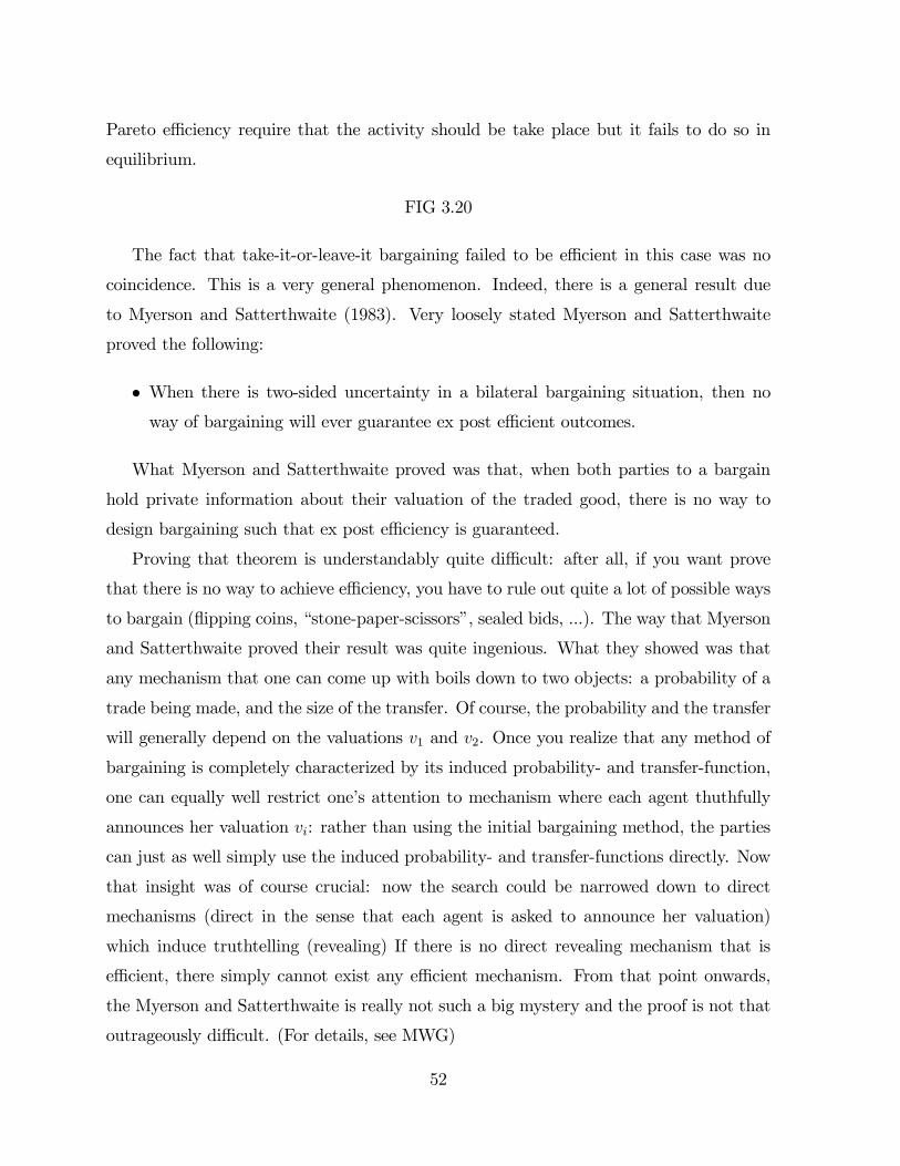
Pareto efficiency require that the activity should be take place but it fails to do so in

equilibrium.

FIG 3.20

The fact that take-it-or-leave-it bargaining failed to be efficient in this case was no

coincidence. This is a very general phenomenon. Indeed, there is a general result due

to Myerson and Satterthwaite (1983). Very loosely stated Myerson and Satterthwaite

proved the following:

• When there is two-sided uncertainty in a bilateral bargaining situation, then noway of bargaining will ever guarantee ex post efficient outcomes.

What Myerson and Satterthwaite proved was that, when both parties to a bargain

hold private information about their valuation of the traded good, there is no way to

design bargaining such that ex post efficiency is guaranteed.

Proving that theorem is understandably quite difficult: after all, if you want prove

that there is no way to achieve efficiency, you have to rule out quite a lot of possible ways

to bargain (flipping coins, “stone-paper-scissors”, sealed bids, ...). The way that Myerson

and Satterthwaite proved their result was quite ingenious. What they showed was that

any mechanism that one can come up with boils down to two objects: a probability of a

trade being made, and the size of the transfer. Of course, the probability and the transfer

will generally depend on the valuations v1 and v2. Once you realize that any method of

bargaining is completely characterized by its induced probability- and transfer-function,

one can equally well restrict one’s attention to mechanism where each agent thuthfully

announces her valuation vi: rather than using the initial bargaining method, the parties

can just as well simply use the induced probability- and transfer-functions directly. Now

that insight was of course crucial: now the search could be narrowed down to direct

mechanisms (direct in the sense that each agent is asked to announce her valuation)

which induce truthtelling (revealing) If there is no direct revealing mechanism that is

efficient, there simply cannot exist any efficient mechanism. From that point onwards,

the Myerson and Satterthwaite is really not such a big mystery and the proof is not that

outrageously difficult. (For details, see MWG)

52

11.3 Multilateral Externalities*

So far we have considered bargaining involving only two parties: an externality gener-

ating party and an affected party. Bargaining becomes more problematic when many

individuals are involved. This is particularly the case for “non-depletable” externalities.

The problem here is that most “solutions” based on bargaining suffer from the same

free-rider problems as voluntary public good provision equilibria.

A Public Bad Example

To illustrate the problem we can look at the case of a firm choosing some action h which

negatively affects a set of individuals. Hence suppose that there is a firm that chooses an

action h (“pollution”) generating net profits π (h).

We will assume that the firm initially has the right to pollute as much as it feel

like it. It then chooses h to maximize π (h). We will then assume that a “market” for

reduction in h is established where the consumers can contract with the firm for marginal

reductions in h. We will consider the competitive case and show that we get a case which

is exactly parallel to the case of under-provision of a public good in the case of voluntary

contributions. Hence initially the firm has the “right to pollute” and hence chooses h0

that solves maxh π (h). There is a set of individuals i ∈ I = {1, 2, ..., n} with identicalquasi-linear preferences over h and “income” x,

φ (h) + x.

With quasi-linear utility it is valid to characterize Pareto optimality as maximizing

the sum of utilities and profits.11 Pareto optimality thus requires that h = h∗ satisfying

π0 (h∗) +Xi∈I

φ0 (h∗) = 0. (62)

The key thing to note is that h should be set so that the marginal profits should

equal the total marginal impact on the consumers’ utilities, i.e. the marginal benefit

11Effectively, since the consumers have quasi-linear utility, social marginal value of a unit of income

is equal to unity. Hence a one pound increase in profits increases total welfare by one unit. Hence the

units are effectively aligned. See MWG, ch. 10.

53

should equal total marginal damage which is obtained by summing over the consumers.

Effectively, this is the Samuelson rule for a public good. We can interpret −Pi∈I φ0 (h) as

the sum of the consumers’ marginal willingness to pay for a reduction in h. This should

correspond to the marginal cost to the firm (in terms of profits) of a reduction in h.

We now establish a “market” where a consumer can buy reductions in h; let p be the

price for a one unit reduction in h. Consider the competitive equilibrium with a price p∗.

The firm (treating p∗ as given) chooses how many units of pollution reduction so trade,

maxh

©π¡h0 − h¢+ p∗hª

where h is the total reduction sold. Thus, at the competitive equilibrium

π0¡h0 − h¢ = p∗. (63)

Let hi denote the number of unit of pollution reduction that individual i’s purchases

reduction, and let h−i =P

j 6=i hi be the total pollution reduction bought by all other

individual other than i. Individual i treats h−i as given (the Nash assumption) and

chooses hi to solve

maxhi

©φ¡h0 − h−i − hi

¢− p∗hiª .Hence at the competitive equilibrium

−φ0 ¡h0 − h¢ = p∗, i ∈ I (64)

where we used that h = hi + h−i for any individual i.

Combining (63) and (64), we see that at the competitive equilibrium

π0¡h0 − h¢+ φ0

¡h0 − h¢ = 0, (65)

which when compared to (62) indicates that h0 − h > h∗ due to free-riding. Hence, dueto free riding, the pollution is not reduced enough to achieve efficiency.

The problem is not exclusive to the case of the competitive solution; it applies equally

well to any case where the consumers are bargaining with the polluter. Each consumer,

when bargaining, will not take into account the effect of the reduction in pollution that

she buys. Hence each consumer will buy too little pollution reduction.

54

11.4 An Empirical Externality: Passive Smoking

As an example of a negative externality we will consider passive smoking. Passive smoking

constitutes a negative externality in that is has been linked to several illnesses such as

lung cancer or heart disease in the adult population. Of particular concern is that passive

smoking affects the health of young children and babies, causing asthma, bronchitis or

sudden infant death syndrome. As a consequence, government have introduced (and are

planning further) policies to limit the exposure of non-smokers and generally to discourage

smoking. A recent study by Adda and Cornaglia (2006) consider the impact of smoking

bans and cigarette taxes in the US on passive smoking.

Measuring Passive Smoking and Data

The damage of smoking is caused by tar and carbon monoxide which is highly correlated

with the nicotine yield of a cigarette. However, nicotine is difficult to measure since it

degrades within few hours of being absorbed. Rather then measure nicotine focuses on

the amount of cotinine, a metabolite of nicotine, which stays in the body longer and can

be measured in an individual’s saliva.

The data used by AC comes from the National Health and Nutrition Examination

Survey, a nationwide representative sample of the US civilian population. Data is from

1988-1994 and 1998-2002. The survey contains information on the cotinine concentration

in both smokers and non smokers, along with information on the number of cigarettes

smoked in the household. In addition the data contains information on the age, sex,

race, health, education and occupation of the individual. Since AC consider the effect of

policy on passive smoking they select as their sample the group of non-smokers (26,997

individuals). They also separate non smokers who share their household with smokers,

from non smokers who live in “smoke free” households.

AC merge this data with information on the smoking regulation in place by year and

by state in different locations. The smoking ban variable is coded on a scale 0-3 measuring

its strictness.12 Moreover, the degree of regulation is measured by type of location: (i)

12Zero if no restriction, one if smoking is restricted to designated areas; two if smoking is restricted to

separate areas; three if there is a total ban on smoking.

55

bars, restaurant and other recreational places, (ii) public transport, (iii) shopping malls,

(iv) work place, and (v) in schools. In addition to measuring bans, AC use information

on (excise) taxes on cigarettes by state and year.

The next figure (Table 1 in AC) provides basic descriptive statistics. It shows that the

vast majority of non-smokers are affected to some extent by passive smoking, although

the measured levels of cotinine is much higher among non-smokers who live is households

with some smoker.

FIG 3.21

Empirical Methodology

The empirical methodology is an extended version of the difference-in-difference approach.

It uses that regulation and taxes have varied across US states and across time. The main

estimating equation can be written as

Cotist = α0 + γRst + βτ st + α1Xist + δs + λt + uist (66)

where Rst is the variable measuring the degree of regulation in state s and year t; τ st

similarly is the log excise tax on cigarettes in states at time t. Individual characteristics

of individual i residing in state s at time t are collected in the vector Xist. δs is a set of

state dummy variables while λt is a set of year dummy variables.

The inclusion of state- and year dummy variables imply that identification of the

effect of regulation and taxes comes from variation across states and time, and not from

cross-sectional differences in the level of state regulations or taxes.13 The identification

of the effect of policy thus relies on the exogeneity of changes in policy within states.

Indeed, over the period studied regulation became more stringent. E.g. n 1991 only 27%

of the states had at least a total ban on smoking in some public space, whereas the figure

13To see how the estimating regression is a generalization of the difference-in-difference approach,

suppose e.g. there only been two states and two years, with one state introducing some regulation

between the two years. In that case the above equation reduces to

Cotist = α0 + γRst + α1Xist + δs=treated_state + λt=after + uist (67)

where the change in regulation Rst = 1 if and only if s = treated_state and t = after.

56

is 51% in 2001. Similarly, excise taxes on increase over the period in question (by on

average increased by 2 cents per year). Hence there is indeed policy variation to allow

identification.

Trends in Passive Smoking

AC first consider the trends in passive smoking. The following two figure (Figure 3 and

4 in AC) graph the trends in cotinine levels for each group of non smokers who live

in “smoke free” households and non-smokers in smoking households, respectively. The

figures are striking. During the period in question tougher policy against smoking was

introduced. This trend in regulation coincides with a downward trend in the level of

cotinine observed in non smokers who live in “smoke free” households. However, this is

not the case for non smokers who share their household with smokers. Hence, despite

the increasing level of severity in regulations and higher excise taxes, it would seem that

tobacco exposure of non smokers living in smoking households did not decrease.

FIG 3.22

FIG 3.23

The authors hypothesize that this may be due to a “displacement” effect whereby,

as a response to bans in certain public places, smokers tend to smoke more inside the

household. This provides a strong justification for exploring the impact of bans in different

locations.

Main Results

Some of the authors main results are highlighted in the following figure (Table 4 in AC).

The table gives the γ coefficient and the β coefficient from running the main estimating

regression. In order to highlight in particular the effect on children, the sample is split

by the age of the individual, grouping together children aged under eight, children aged

8-12, children aged 13-20, and those over 20.

FIG 3.24

57

The results are striking: the effect of bans on smoking in bars, restaurant and other

recreational places (“going out”) significantly increases the cotinine level in children up

to the age of 12 (the estimated effect of 0.65 for children under the age of 8 corresponds

to smoking 1/20 of a cigarette), clearly suggesting a displacement effect whereby smokers

smoke more inside the household. In contrast banning smoking in shopping malls have

the (intended) effect of reducing passive smoking by children. The table also shows that

increasing the tax on cigarettes reduces passive smoking by children.

References

Adda, J. & Cornaglia, F. (2006), ‘The effect of taxes and bans on passive smoking’,

Mimeo, University College London.

Andreoni, J. (1988), ‘Privately provided public goods in a large economy: The limits of

altruism’, Journal of Public Economics 35, 57—73.

Andreoni, J. (1989), ‘Giving with impure altruism: Applications to charity and ricardian

equivalence’, Journal of Political Economy 97, 1447—58.

Andreoni, J. (1990), ‘Impure altruism and donations to public goods: A theory of warm

glow giving’, Economic Journal 100, 464—477.

Andreoni, J. (1993), ‘An experimental test of the public-good crowding-out hypothesis’,

American Economic Review 83, 1317—1327.

Andreoni, J. (1995), ‘Cooperation in public goods experiments; kindness or confusion?’,

American Economic Review 85, 891—904.

Andreoni, J. & Bergstom, T. (1996), ‘Do government subsidies increase the private supply

of public goods?’, Public Choice 88, 295—308.

Bergstrom, T., Blume, L. & Varian, H. (1986), ‘On the private provision of public goods’,

Journal of Public Economics 29, 25—49.

58

Bergstrom, T., Blume, L. & Varian, H. (1992), ‘Uniqueness of nash equilibrium in private

provision of public goods: An improved proof’, Journal of Public Economics 49, 391—

92.

Bergstrom, T. & Varian, H. (1985), ‘When are Nash equilibria independent of the distri-

bution of agents’, Review of Economic Studies 52, 715—718.

Bernheim, D. (1986), ‘On the voluntary and involuntary provision of public goods’, Amer-

ican Economic Review 76, 789—793.

Bliss, C. & Nalebuff, B. (1984), ‘Dragon slaying and ballroomdancing: The private supply

of a public good’, Journal of Public Economics 25, 1—13.

Coase, R. (1960), ‘The problem of social cost’, Journal of Law and Economics 1, 1—44.

Cornes, R. & Sandler, T. (1996), The Theory of Externalities and Clubs, Cambridge

University Press.

Kingma, B. (1989), ‘An accurate measurement of the crowd -out effect, income effect and

price effect for charitable contributions’, Journal of Political Economy 97, 1197—

1207.

Marwell, R. & Ames, R. (1981), ‘Economist free ride - does anyone else?’, Journal of

Public Economics 15, 295—310.

Mas-Colell, A., Whinston, M. & Green, J. (1995), Microeconomic Theory, Oxford Uni-

versity Press.

Meade, J. (1952), ‘External economies and diseconomies in a competitive situation’, Eco-

nomic Journal 62, 54—67.

Myerson, R. & Satterthwaite, M. (1983), ‘Efficient mechanisms for bilateral trading’,

Journal of Economic Theory 29, 265—281.

Payne, A. (1998), ‘Does the government crowd -out private donations? new evidence

from a sample of non-profit firms’, Journal of Public Economics 69, 323—345.

59

Pigou, A. (1932), The Economics of Welfare, MacMillan, London.

Samuelson, P. A. (1954), ‘The pure theory of public expenditure’, Review of Economics

and Statistics 36, 387—389.

Samuelson, P. A. (1955), ‘Diagramatic exposition of a pure theory of public expenditure’,

Review of Economics and Statistics 37, 350—356.

Varian, H. (1992), Microeconomic Analysis, 3’rd edn, W.W. Norton.

60