1  

 

Market equilibrium and the environmental effect of tax

adjustments in China’s automobile industry  

Junji Xiao

 

School of Management

Fudan University

 

Heng Ju 

 

School of International Business and Administration

Shanghai University of Finance and Economics

 

2011‐3‐20 

 

                                                               Corresponding author. Email: junjixiao@fudan.edu.cn. We are indebted to Shanjun Li for discussion on the rough idea of this project. We also thank Matthew Shum, Weimin Hu, Xiaolan Zhou and other participants at Five Star Forum, who made very help comments on this paper. All remaining errors are ours. 

2  

Market equilibrium and the environmental effect of tax

adjustments in China’s automobile industry

Abstract

This paper explores the effects of consumption and fuel tax regime adjustments on

China’s auto industry. Applying the model and simulation method of Berry, Levinson,

and Pakes (1995), we conduct a comparative static analysis of equilibrium prices and

sales, fuel consumption, and social welfare before and after tax adjustments. Further,

for the first time, we compare the progressivity of both taxes. Our empirical findings

suggest that fuel tax lowers vehicle consumption and consumer surplus more than

consumption tax does, but our conclusion about the environmental effects of both

taxes depends on the assumption of the fuel efficiency of outside fleets.

Keywords: China auto industry, welfare analysis, environmental effect, BLP model,

tax progressivity

I. Introduction

China’s automobile industry has developed rapidly in the last two decades. In 2009,

China overtook the United States as the biggest auto market; the passenger car sales

soared to 10.3 million, and the total vehicle sales were estimated at 13.6 million.

However, a concomitant of this rapid development is the serious air pollution and

carbon dioxide (CO2) emission. With its annual CO2 emission in 2007 accounting for

22.3% of the global total, China heads the list of sovereign states and territories on

this score1. Meanwhile, emissions from motor vehicles have become the main source

3  

of air pollution in China’s large- and medium-sized cities, according to the China

Vehicle Emission Control Annual Report 2010 by the Ministry of Environmental

Protection. This report shows that the volume of pollutants generated by motor

vehicles across China in 2009 amounted to 51.4 million tons, with cars contributing

most of it. Furthermore, Walsh (2000) also estimated that mobile sources contributed

approximately 45–60% of the NOx emissions and about 85% of the CO emissions in

major Chinese cities.

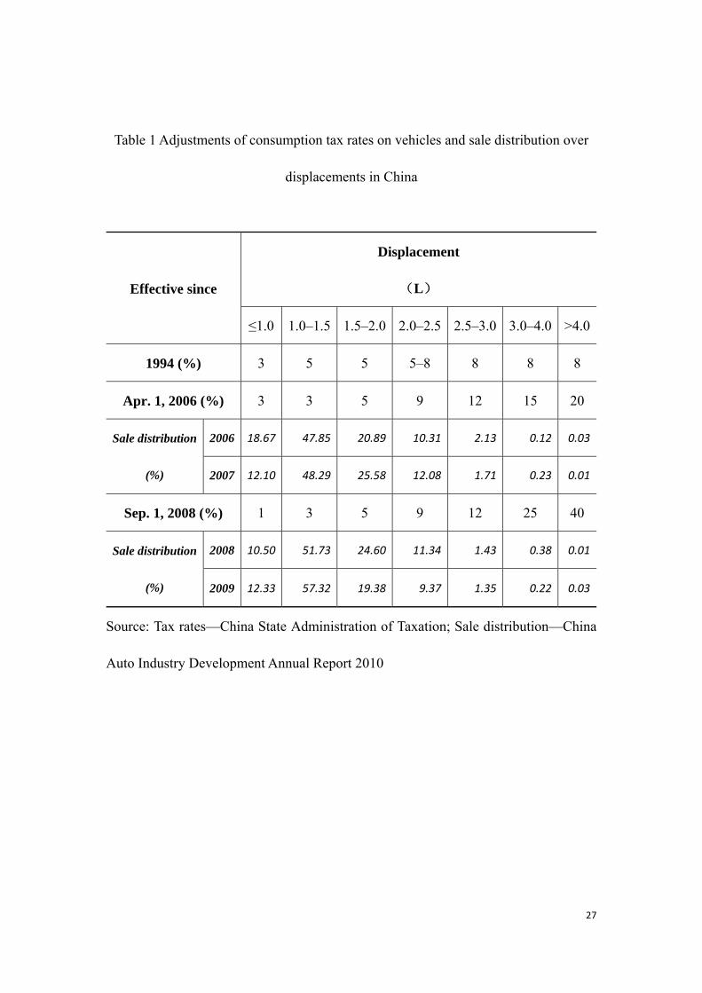
To reduce automobile emissions, China’s Ministry of Finance and the State

Administration of Taxation adjusted the consumption tax on vehicles twice, on Apr 1,

2006, and Sep. 1, 2008 (Table 1). In short, these policy adjustments raised the

consumption tax rates on passenger vehicles with high displacements but lowered the

rates on those with small engines2. Obviously, the purpose of this adjustment was to

discourage high-emission cars and promote small ones, in an effort to reduce pollution

and save energy. From the observed sale distribution changes over the years, as shown

in Table 1, these tax adjustments raised the ratio of cars with engine size smaller than

2 liters, while shrinking the ratio of cars with larger displacement; thus, it would

appear that the adjustments produced the intended effect. Meanwhile, other

exogenous variables, such as gasoline price, product quality, and the number of car

models, also changed, which may exaggerate or understate the effects of the taxation

scheme changes on sale distribution. This calls for a formal investigation taking into

account these exogenous changes.

This paper investigates the environmental effects of these tax scheme adjustments by

4  

conducting comparative static analysis on total fuel consumption and fleet average

fuel efficiency3. We employ the model and simulation method of Berry, Levinson, and

Pakes (1995; hereafter BLP) to obtain the equilibrium fuel consumption and fleet

average fuel efficiency in a counterfactual tax scenario, and compare them to their

actual counterparts. On the other hand, previous studies show that an effective

emission-abatement policy is costly (Greene and Liu 1988, Crandall and Graham

1989, Kleit 1990, and Crandall 1992 for Corporate Average Fuel Economy [CAFE]

and fuel tax, and White 1982 and Bresnahan and Yao 1985 for air-pollution standards

of the Clean Air Act). Accordingly, we calculate the social welfare loss in new-car

markets to measure the costs of tax changes4. To illustrate the effects of the

consumption tax adjustments, we use a hypothetical fuel tax for comparison5.

Our study shows that neither consumption tax nor fuel tax lowers the

market-share-weighted average fleet fuel consumption significantly. However, fuel

tax leads to a decrease in the total sale of new cars, which in turn leads to a decline in

the total fuel consumption from new cars. It does not change the sale distribution over

various fuel efficiency models. On the contrary, consumption tax adjustment skews

the sale distribution toward more efficient new cars, and increases the total fuel

consumption due to increased sales. The effects of these two taxes on environment

depend on our assumption about the average fuel efficiency of outside goods. Further,

the social welfare loss due to consumption tax is relatively less—in particular, the

decrease in consumer surplus is less by an order of magnitude, in comparison to the

fuel tax. Fuel tax actually transfers more welfare from private sector to the

5  

government.

The effectiveness of various emission-reduction policies has attracted attention from

both policymakers and researchers for a long time. Most extant literature compares

the tax policies such as fuel tax (Dahl 1979; Parry and Small 2005; Fullerton and Gan

2005; Feng, Fullerton, and Gan 2005; Bento et al. 2009), and other compulsory

non-tax regulations such as CAFE (Crandall 1992; Sterner, Dahl, and Franzén 1992;

Koopman 1995; Agras 1999; West 2004). Although ambiguous conclusions have been

drawn on their effectiveness, most studies have found that fuel tax is more efficient in

decreasing the Vehicle Miles Traveled (VMT), while CAFE is efficient in improving

the average fuel economy of new cars6. However, few empirical studies to date have

estimated the environmental and welfare effect of an excise tax on the car. China’s

automobile consumption tax is such an excise tax, with rates varying according to

engine size. This tax is not as stringent as CAFE. Manufacturers do not need to

restrict their average fuel efficiency; instead, they can choose to share some tax

burdens to sustain their market shares. In this way, manufacturers partially internalize

the marginal social cost of less fuel efficiency, rather than downsize the cars to satisfy

the compulsory requirement7. Therefore, this tax may be a favorable policy to solve

the safety issues due to CAFE. This paper is the first study to empirically investigate

the efficiency and cost of this tax.

This paper differs from the previous studies in the following aspects. First, China’s

automobile consumption tax on displacement is unique8, and this is the first paper to

investigate the consequence of this tax and compare it to the fuel tax. This tax scheme

6  

sets progressive tax rates over displacement tiers, so tax payment is based on both

displacement tiers and car values. Fullerton, Gan, and Hattori (2004) studied a similar

annual automobile tax levied by the prefecture governments of Japan. Japanese

automobile tax is a list of flat amounts over tiers of displacement, invariant to car

value. China’s tax scheme is more effective in reducing the sales of large cars than the

lump-sum tax varying according to displacements, since car values are positively

correlated with displacement. Besides, in terms of fairness, such a tax scheme is more

progressive than the lump-sum tax scheme. This paper estimates the progressivity of

the consumption tax, and compares it to that of the fuel tax.

Second, this paper simultaneously estimates the impacts of tax adjustment on both the

demand and supply sides, while most empirical studies to date have focused on the

demand side estimation (Greene and Liu 1988, Bento et al. 2009, West 2004). The

BLP (1995) framework models the price competition among manufacturers, so it can

be used to analyze the profit variation as well as consumer surplus changes due to

exogenous tax changes, which makes this study capable of estimating the total social

welfare changes rather than only consumer surplus changes.

Third, the empirical model in this study endogenizes the response of the equilibrium

automobile prices to tax changes. The previous research usually ignores this while

studying the effectiveness of emission-reduction policies (Fullerton, Gan, and Hattori

2004; West 2004). Since firms are heterogeneous in their costs, they may respond

quite differently to a tax policy change. Firms with lower productivity have to pass on

all the tax addition to consumers, while those with higher productivity can absorb

7  

some tax burden to sustain sales. Without considering the competition effect on car

prices, the consumer welfare loss due to a tax change may be overestimated9. This

paper investigates the tax incidence and finds that large-displacement car makers do

share some tax burden to sustain their market share. Therefore, by incorporating this

endogeneity, our estimates of welfare and environmental consequence add more

precise evidence to the literature.

The rest of the paper is organized as follows. Section II briefly introduces the

automobile industry and the consumption tax system in China. Section III lays out the

empirical model and estimation method. Section IV describes the data and summary

statistics. Section V presents the empirical results of the model estimation and

counterfactual experiments. Finally, section VI presents a summary.

II. Description of the automobile industry and tax adjustments

China’s automobile industry

Over the last two decades, China’s automobile industry has witnessed a rapid

development. With new car sales of 13.6 million in 2009 and a vehicle population of

62 million at the end of the year, China became the largest auto market in the world10.

The development of this industry is asymmetric; in particular, the market share of

passenger vehicles has increased from 8.3% in 1990 to 75.7% in 2009, while the

market share of trucks declined from 52.8% to 16.5%, reflecting a switch in this

industry to private cars11.

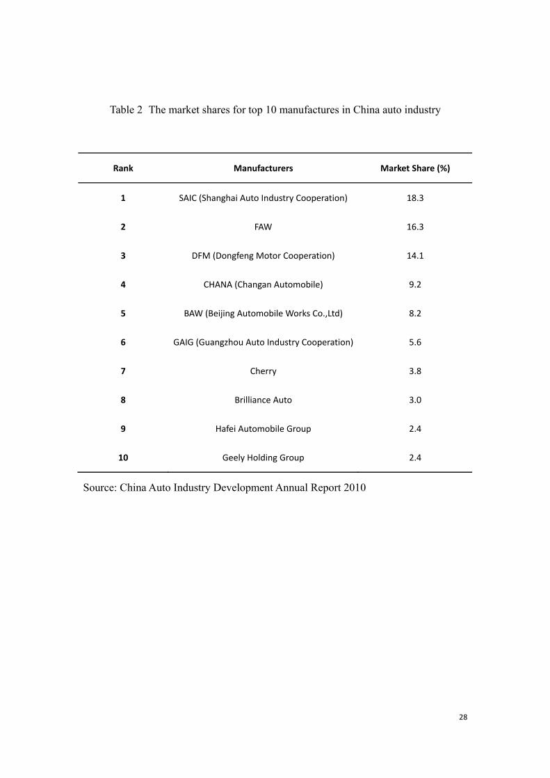
The automobile industry of China is highly competitive due to the entrance of new

manufacturers and further deregulation required by the WTO agreement (Deng and

8  

Ma 2010). There are 171 manufacturers in this market, and the total market share of

the five largest firms accounted for 66.1% of sales in 2008 (see Table 2 for details).

Among the top ten manufacturers, eight are joint ventures with foreign car makers:

Volkswagen, BMW, Mercedes Benz, General Motors, Hyundai, Nissan, Honda, and

Toyota. Local brands accounted for only 25.92% of the market in 2008. Figure 1

displays the joint-ownership structure of China’s automobile market. The complex

market structure and the nature of multi-ownership for the top manufacturers make it

difficult for them to collude with each other12. Therefore, we choose a strategic

competition framework to model this market.

Our empirical analysis focuses on the light-duty passenger vehicle market, consisting

of the sedan, MPV, and SUV. This market accounts for 75.3% of the total vehicle

production in China. Most of the production is for domestic consumption. In 2008, the

export of light-duty passenger vehicles was 0.24 million, which is less than 4.8% of

the total production13. The import was about 0.15 million, which is negligible.

The consumption tax system and fuel tax

In China, a car attracts three categories of taxes: the consumption tax, the value-added

tax (VAT), and the vehicle purchase tax, paid by the manufacturers, retailers, and

consumers, respectively, although almost all taxes will be transferred to the consumers

finally. The consumption tax came into being in 1994 targeting high-value or

high-resource-consuming goods. For car sales, the tax rates vary with the

displacement tiers (Table 1). VAT has been fixed at 17% since 1993 for the entire

retailing sector. Vehicle purchase tax has also been fixed at 10% since 2001 for all

9  

passenger vehicles as of 2010. The calculation formula for these three taxes is given

below:

(1+ ) (1+ ) =

(1+ )

m c r

m c v

p t t p

Vpt p t t

where, ct , vt , and rt are the rates for consumption tax, vehicle purchase tax, and

VAT, respectively, mp is the wholesale price to dealers, p is the list price to

consumers, and Vpt is the vehicle purchase tax that consumers pay on top of the

VAT-deducted list price. Since vehicle purchase and VAT rates do not vary with

different car models and stay unchanged over time, we ignore their impact in our

study.

The fuel tax took effect in January 2009, 15 years after the debate on the tax started in

199414. Since air pollution has become a significant concern in China, the government

finally decided to implement the fuel tax to facilitate energy saving and emission cuts

as well as economic structural adjustments. Based on the price for 93# gasoline in the

mass market, the tax rate is close to 30%.

III. Empirical model and estimation method

Empirical framework

Consumers are assumed to choose a car from N models to maximize their utilities.

The indirect utility function for consumer i purchasing product j is as follows:

( ) ( ) ( )

( ) _

i i i ij ge ge ge j pw pw pw j wg wg wg j

i i ip p p ge j br j j j

u const v GE v POWER v WEIGHT

v inc PRICE BR DUM

This indirect utility function assumes that consumers will compare the characteristics

of the cars in their choice set. Some key car features, such as horsepower (POWER),

10  

weight, price, fuel efficiency, and the place of origin of their brands (BR_DUM) are

observable, while other features are not. Therefore, we use j to indicate those

features consumers will consider while making their purchase decision, but are not

observable in our data, and assume it follows a distribution with mean zero. Given the

fact that consumers usually evaluate fuel efficiency in the same way as expenditures

on gas, it is assumed that their utility depends on gas expenditure (GE), which is the

product of fuel consumption and gas price measured in Chinese currency RMB

yuan/liter, rather than fuel efficiency. By its construct, GE records consumers’

expenditure on gas for a 100-km drive. If the average driven distance for a

representative consumer is standardized to 100 km per year, GE actually measures the

total expenditure of a representative consumer on gasoline per year. Since consumers

are heterogeneous in their driving patterns, we take into account this difference using

variable igev , which is the ratio of an individual’s idiosyncratic driven distance to the

mean level. Similarly, individuals have idiosyncratic tastes on the other product

characteristics; we denote these taste variations on power, weight, and price using

ipwv , i

wgv , and ipv , respectively. Model parameters , , describe the

consumer’s preference on the car characteristics. Finally, we assume that the

idiosyncratic consumer taste ij follows a traditional type I extreme value

distribution; therefore, the probability for consumer i to choose product j is given as

0

, ,

ij

ik

ui i

ij j Nu

k

eS x v inc

e

, where jx is a vector of all product characteristics.

The market share for product j is given as

11  

, , , ( ) ( )i ij j ij j

B

S x S x v inc dP v dP inc (1)

where B is the set of consumers whose idiosyncratic tastes and income drive them to

purchase product j.

On the supply side, manufacturers conduct differentiated Bertrand competition, so the

profit maximization problem for manufacturer f producing fJ models can be

formalized as

max ( ) ,1f

jf j j j

p j Jj

pmc MS x

t

 

Here, market size M is constant. Since car models with different displacements are

exposed to different tax rate jt , the net income for manufacturers is 1j

j

p

t. The

marginal cost jmc does not change in output, but it varies across different car models;

therefore, it is a function of product characteristics jw :

ln( )j j jmc w

Since this function is in the log-linear form, the parameters indicate the

percentage change of marginal costs due to a particular car characteristic change.

The first-order condition of the profit maximization problem gives the following

equation:

ln( ( , , )) ln(1 )

jj j j j

j

px t mc w

t

(2)

where, ( , , )j x t is the markup of product j, and it should be a function of demand

side variables, parameters, and taxes for all car models. Equations (1) and (2) give rise

to the equilibrium conditions in the market.

Estimation issues

12  

We apply the GMM estimation method proposed by BLP (1995) to estimate the

parameters in equations (1) and (2) simultaneously. In short, we use the observed

market share to recover the mean utility in equation (1), which is a function of

consumers’ mean preference , the observed product characteristics, and unobserved

product characteristics j . Then, our moment condition is ( , , )

0( )

E Z

,

where Z is a set of instrumental variables described below. For the details of this

method, readers can refer to BLP (1995). We will only discuss relevant issues

involved in the estimation process.

One important issue of this method is the computation of aggregate market shares.

Following Nevo (2001), we make ns random draws from standard normal distribution

to simulate the idiosyncratic consumer tastes, and make the same amount of random

draws for a vector of household income and annual driven distance based on survey

data. These random values are used to calculate the conditional choice probability for

each individual, and then the unconditional market shares are derived using the

average of the individual market shares given by 1

1, , ,

nsi i

j j ij ji

S x S x v incns

.

Another issue is the choice of instrumental variables for the price endogeneity

problem. In this study, we use three sets of instrumental variables: the product

characteristics, the sum of corresponding characteristics over all the firms’ other

models, and sum of product characteristics over other firms’ car models in a market.

Nevo (2001) shows that these are valid instrumental variables that are independent of

the unobservable characteristic terms but correlated with prices.

13  

Finally, given the estimates of structural parameters, we use compensating variation

(CV) to calculate consumer surplus changes due to tax changes. For a logit discrete

choice model on the demand side, Nevo (2000) shows that CV can be calculated as

follows:

, ,0 0

1

ln{ exp } ln{ exp }

( )

N Ni ij post j prens

j j

i ii p p p ge

u uM

CVns v inc

 

IV. Data and summary statistics

This section describes three main sources of data used in this paper: (1) monthly car

model sales from China Association of Automobile Manufacturers (CAAM); (2)

product attributes collected from Car Market Guide; and (3) consumer demographic

characteristics from a survey conducted among vehicle owners in Beijing by

Guanghua School of Management at Beijing University of China in 2005. The

summary statistics are listed in Tables 3 and 4.

Monthly sale and price data from January 2004 through December 2008 are available

from CAAM. Since the car feature data for 2006 are missing, we have to drop the

sales data for 2006 in our estimation. The total sale of car models for 2008 in our

sample is 5.49 million, which accounts for 81.3% of the total passenger vehicle sales

in the China market. To derive the market share for each car model, we set the market

size at the number of city households who owned a house with more than three rooms,

published in the Fifth National Population Census (2000) by the National Bureau of

Statistics of China. This number is 17,963,39915.

A stylized fact is that most entry and exit of car models occurred in January or some

14  

month in the second half year. In other words, the competition structure over half-year

intervals is quite stable. Therefore, we aggregate the data into half-year levels and use

the average monthly prices and sales for each half year to measure their sales and

price. In this way, we can include the truncated data and make a comparison across

1297 car models. Large variations in both sales and prices are observed. The most

popular car model has a monthly sale of over 19,000 units, while the minimum sale is

only 12 units per month. The standard deviation in price is 123311.7, which is high

relative to the average price of RMB 168454.8.

Product features are reported in the Car Market Guide. We define a car model by the

product characteristics, including brand and the following model features.

Horsepower is measured by kilowatts. jWEIGHT is the logarithm of the car weight

measured in kilograms. Fuel consumption is a ratio given in liters/100 km, which is

used to construct the gas expenditure variable as described in the model section.

Place-of-origin dummy variables for brands show that European, Japanese, and

American cars are most popular in China.

Household income is reported as categorical data in interval scales as listed in Table 5.

We use the average of each interval to represent the income of consumers falling into

that interval. For the first and last interval, we choose RMB 1,000 and 100,000,

respectively. In this way, the average household income corresponding to the mean

statistics in Table 3 amounts to RMB 8,300 per month16. The average distance

traveled per year by Beijing car owners is about 22,000 km, and 60% of the drivers

traveled less17. This supports our intuition that the main purpose of purchasing a car is

15  

for daily commute in China. Therefore, the driving pattern is relatively inelastic to

some exogenous shocks such as fuel price changes. These survey data are used to

simulate the consumers in the China auto market. Considering the computation

burden, we finally randomly draw a thousand vectors of these two variables to

represent individuals’ demographic information.

V. Empirical results

In this section, we will first present the estimation results; then, we will report the

empirical results for a counterfactual experiment to illustrate the impact of both

consumption and fuel tax.

A. Estimation results

Estimates of the model parameters are listed in Table 6. All estimates for the mean

utility function are significant with expected sign. Consumers prefer more powerful

and larger size but less-fuel-consuming cars. These findings coincide with most of the

previous research (Bresnahan 1987, Greene and Liu 1988, BLP 1995, Deng and Ma

2010). In particular, the statistic on driving distance shows that VMT is relatively

inelastic in China; hence, it is assumed unchanged with vehicle choice and other

exogenous factors such as fuel price. Therefore, the variation in fuel expenditure on

different car models reflects the physical difference in cars’ fuel efficiency. The

negative coefficient of fuel expenditure shows that efficient cars are more favorable.

On the cost side, all estimates are significant. Unlike the demand side, fuel

consumption rather than fuel expenditure is incorporated into the marginal cost

function. This is because cost per se only depends on the car features and production

16  

technology, but not on fuel prices. A negative sign indicates that a

more-fuel-consuming car costs less than a fuel-efficient car. Coefficients of brand

dummies are also positive and significant. This may imply that foreign brands invest

more than local brands on characteristics other than those included in our analysis.

Almost all the estimates for the idiosyncratic tastes and household demographic

variation are insignificant, implying consumers are not so different in the car features

in our study. However, consumers do show variation in their sensitivity to price,

although the estimate for the standard deviation on the tastes for price (-0.1105) is less

than one-third of that for price in the mean utility (-0.3894). Estimation results also

show that households with higher income are less sensitive to price changes, but this

effect is not significant.

B. Counterfactual experiments

While studying the effectiveness and welfare effect of tax changes, it is necessary to

control for the market structure changes and keep technical surface unchanged before

and after tax changes. However, associated with tax changes, new entry of car models

is observed. To disentangle the tax effect on the equilibrium prices and market shares

from changes in competition environment, we conduct a counterfactual experiment

using the data for September to December 2008, during which period there were 252

car models in the market. We assume that the market structure is unchanged and that

the tax scheme is set as it was before the tax adjustment in April 2006; we then solve

the equilibrium prices and market shares. Similarly, we also solve the equilibrium set

for a scenario in which gasoline is subject to a 30% fuel tax, while assuming the

17  

consumption tax scheme remained unchanged.

a). Equilibrium price analysis

Figure 2 displays the simulated tax-inclusive price changes before and after tax

adjustments. Apparently, the price of most fuel-efficient cars declines after the

consumption tax adjustment, while the price of high-fuel-consuming cars increases

dramatically. However, a similar trend is not observed for fuel tax. On the contrary,

manufacturers of fuel-consuming cars either undercut their prices or keep them

unchanged to compete with efficient cars after fuel tax.

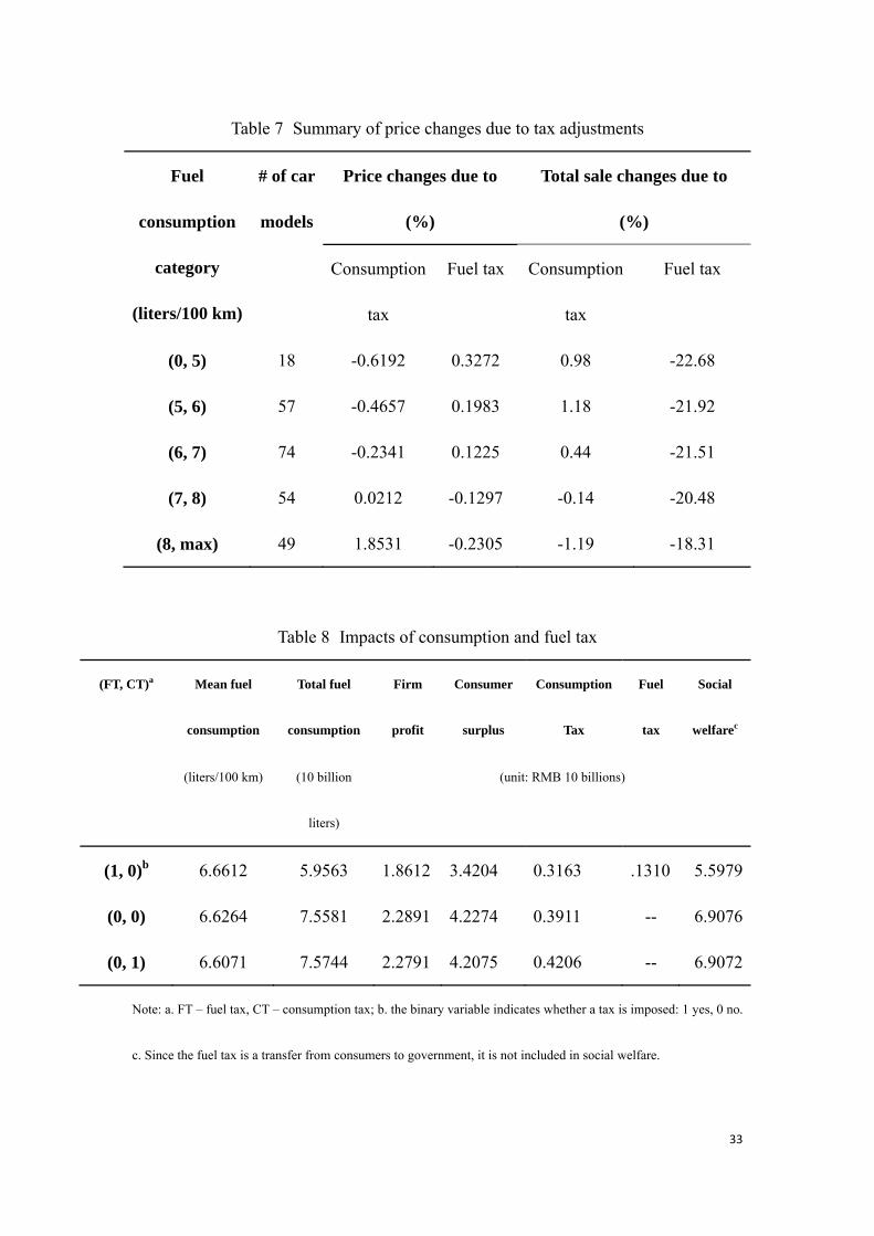
A summary of price changes is listed in Table 7. Cars are categorized into various

groups by fuel consumptions; then, we calculate the average price changes due to tax

adjustments for each group. Consumption tax adjustment is embodied in the auto

prices: the average price for efficient cars is lowered since the consumption tax rate

for this section is lowered, while the average price for fuel consuming cars increases

due to a higher consumption tax rate. Although manufacturers have already shared

some tax burden (we will show the tax incidence below in detail), they have no

capability to absorb all the tax, so the final prices for inefficient cars increases by a

notable scale. Fuel tax causes an adverse pattern in price changes. The reason is that

fuel tax affects fuel expenditures on different car models disproportionally. It raises

the fuel cost on inefficient cars much more than on the efficient models. To sustain

their market share, the manufacturers of fuel-consuming cars have to lower their

prices. On the other hand, the efficient cars obtain advantage after fuel tax, so they

can charge higher prices.

18  

b). Tax incidence

Before investigating the welfare effect of tax adjustments, we analyze the tax

incidence first since this will give a rough picture about welfare transfer between

consumers and manufacturers.

Since the tier of tax rates is set by displacement levels, we plot the percentage change

of tax-inclusive prices versus car displacement in Figure 3. For cars with displacement

lower than 1.5 liters, their effective tax rate is lower after adjustment. Consequently,

we observe a negative change in price for most car models in this category. For cars

with displacement between 1.5 and 2.5 liters, their tax-inclusive prices are not

supposed to change since they are exposed to barely changed tax rates. However, the

intensive competition in this category drove the prices of most models down more or

less. Therefore, actually manufacturers in this segment shared some tax burdens. For

cars falling into the category of 2.5–3, 3–4, and above 4 liters, we expect their

tax-inclusive price to increase by 4%, 16%, and 30%, respectively, if manufacturers

do not share any tax burden. Figure 3 shows that most manufacturers for cars below 4

liters just passed on the tax burden to consumers directly. Only those producing large

cars shared moderate taxes to sustain their market shares. Therefore, we expect to see

consumers lose more than the producers from tax rate increases.

c). Impact on fuel consumption and welfare analysis

The environmental effects of these two tax adjustments are expected to be different.

Since the tax-inclusive prices benefit efficient cars in their market shares under

consumption tax adjustment, the market share-weighted average fuel consumption is

19  

expected to decrease for this case. However, it is ambiguous as regards fuel tax since

the price changes reversely to the fuel expenditure. We summarize the share-weighted

average fuel consumption in the first column in Table 8.

Our results show that neither fuel tax nor consumption tax has a significant effect on

fuel efficiency18. However, the average fuel consumption decreased by 0.2% after

consumption tax adjustment, while the average fuel consumption increased by 0.5%

after fuel tax adjustment.

An interesting finding is that the total consumption of fuel under various scenarios

displays completely opposite trends (column 2)19. Fuel tax reduces total consumption

of fuel by 16 billion liters, while consumption tax leads to an increase by 0.16 billion

liters. How should the result on fleet average fuel consumption be reconciled with that

on the total fuel consumption? To answer this question, we need to look into the

definition of these two measurements. The fleet average fuel consumption is a

sale-weighted average fuel consumption conditional on purchase; therefore, when the

realized total sale decreases on a relatively larger scale than the average fuel

consumption does, then the conditional average increases. In the case of fuel tax,

consumptions on all fuel efficiency levels have dropped after tax since the

expenditure on gas go beyond consumers’ budgets, leading to sharp decline of total

sale of cars, while the sale distribution over fleet average fuel consumption does not

change much (column 6 in Table 7). In the case of consumption tax, however, the

decreased tax rate for the small-displacement cars attracted more sales, leading to an

increase of total sales, while the sale distribution skewed to efficient cars (column 5 in

20  

Table 7). Therefore, we observe a decrease in the total consumption of fuel due to the

decline of fleet size and an increase of average fuel consumption due to the drop in

marginal consumers under fuel tax, but observe completely opposite trends under

consumption tax.

A natural question arises: Which measurement should we use to make a judgment on

the policies? The answer to this question depends on the assumption of the outside

goods. When a consumer chooses not to purchase a car in our dataset, he may choose

not to purchase, in which case his fuel consumption is zero, or to purchase a used car

or any car outside of our data, in which case his fuel consumption may be even higher.

Given the unavailability of used-car data, we calculate the thresholds of fleet average

fuel consumption for the outside goods, which makes the total consumption of fuel

under the scenario of both tax adjustments indifferent to each other, using the

following equation:

* *(1 )* * *(1 )*f f c cn o j n o j

j j

TFC AMT AFCO S M TFC AMT AFCO S M

where, fnTFC and c

nTFC are the total fuel consumption for new cars subject to fuel

tax and sale tax, respectively (as shown in column 3), AMT is the average distance

traveled, AFCO is the average fuel consumption of outside goods, (1 )fj

j

S and

(1 )cj

j

S are the market shares of outside goods under fuel and consumption taxes,

respectively. Since AMT is available from our demographic data sample, AFCO

can be solved from the above equation. Similarly, we solve the threshold of average

fuel consumption for consumption tax to reduce total consumption of fuel relative to

the no-tax case.

21  

Figure 4 illustrates the savings in total consumption of fuel under both taxes. Our

results show that when the average fuel consumption for the outside goods is above

3.30 liters/100 km, consumption tax is effective to lower the total consumption of fuel,

compared to the case without tax; when it is below 6.62 liters/100 km, fuel tax can

save total consumption of fuel. When the average fuel consumption of the outside

goods is below 6.55 liters/100 km, fuel tax works better than consumption tax in

lowering total consumption of fuel. Intuitively, if consumers who choose the outside

options are more likely to purchase an inefficient car, then policy leading to less total

sale of new cars will become worse even if it saves the consumption of fuel on new

cars. For instance, assuming the average fuel consumption for used cars is 10

liters/100 km, then only if the chance for an outside-goods consumer to choose a used

car is below 65.5% will fuel tax become more efficient than consumption tax.

On the other side, both taxes lead to consumer welfare loss, but they are quite

different in magnitude and welfare re-distribution (columns 3–6). The welfare loss

due to consumption tax adjustment (4 million) is about four orders of magnitude less

than that caused by fuel tax (13.1 billion). More importantly, fuel tax leads to a

consumer welfare loss (8.07 billion) in an order of magnitude more than the loss from

consumption tax (199 million). The same pattern is observed in the manufacturers’

profit, while the government’s tax income increases by 562 million from fuel

consumption, even using the number of fuel tax for one year. In other words, both

taxes result in welfare re-distribution among economic principals, but fuel tax

transfers welfare from the private sector to the government in a much larger

22  

magnitude.

d). Tax progressivity

Policy makers are usually concerned about the distributional effect of a tax. Most

economists and policy makers support a progressive tax system, since “it is not very

unreasonable that the rich should contribute to the public expense, not only in

proportion to their revenue but something more”20. To measure the progressivity, we

construct the Lorenz curves proposed in Suits (1977). Figure 5 illustrates the

distributional effect of both taxes over household incomes. It shows that the

percentage of tax burden borne by the lowest income groups is higher than their share

of total income for both taxes, so the curves arch above the diagonal equity line,

which is similar to the sales and excise taxes in the states shown in Suites (1977).

Our findings coincide with those of West (2004) in that both consumption tax and fuel

tax are regressive 21 . However, West (2004) finds that gas or miles taxes are

significantly less regressive than size taxes, but our findings suggest that consumption

tax based on the size of displacement is less regressive than fuel tax for the lower

income group but the effect is the opposite for the higher income group.

VI. Conclusion

We found that fuel tax is more costly than sales tax in increasing the fuel efficiency

level because consumption tax leverages tax payment on different displacement types

of automobiles: subsidizing small-displacement cars with tax income from large cars,

while fuel tax equates the marginal costs of reducing fuel consumption across all uses

(Crandall 1992). Therefore, the consumption tax is more efficient to induce

23  

consumers to choose fuel-efficient cars, making the sale distribution skewed toward

efficient cars; the sale distribution over fuel efficiency remains unchanged in the case

of fuel tax adjustment. However, fuel tax decreases the total sale of new cars, while

consumption tax adjustment actually enlarges the total sale a little bit. Therefore, they

have the opposite effect on the total consumption of fuel. Their total effects on the

environment, however, depend on the average fuel efficiency of the outside goods. As

long as the proportion of outside-goods consumers who finally purchase a

high-fuel-consuming car is not large, the fuel tax works better in lowering the total

consumption of fuel.

Our fairness study shows that consumption tax is less regressive than the fuel tax for

low-income consumers. Moreover, it does not reduce consumer surplus as much as

fuel tax does. Nevertheless, considering the externality of savings in fuel consumption,

the welfare loss due to fuel tax should be much lower.

However, our conclusion relies on one assumption: we assume the driving pattern will

not change even when consumers are exposed to a 30% fuel tax. Considering the fact

that the main purpose of driving in China is business transportation, this assumption is

reasonable. Kahn (1996) finds that “emissions reduction has occurred even though

total vehicle miles travelled has more than doubled,” and his explanation about this

phenomenon is that emissions fall when new-car emissions regulation becomes more

stringent. This also supports our assumption about travel pattern, since his finding

proved that regulation on fuel efficiency is more efficient than policies affecting

driving patterns in reducing emissions.

24  

References

Agras, Jean. 1999. “The Kyoto Protocol, CAFE Standards, and Gasoline Taxes.”

Contemporary Economic Policy. 17(3): 296-308.

Bento, Antonio M., Lawrence H. Goulder, Mark R. Jacobsen, and Roger H. von

Haefen. 2009. "Distributional and Efficiency Impacts of Increased US Gasoline

Taxes." American Economic Review, 99(3): 667–99.

Berry, Steven, James Levinsohn and Ariel Pakes. 1995. “Automobile Prices in Market

Equilibrium.” Econometrica, 63(4): 841-890.

Bresnahan, Timothy. 1987. “Competition and collusion in the American automobile

market: the 1955 price war.” Journal of Industrial Economics, 35(4): 457-482.

Bresnahan, Timothy and Dennis A. Yao. 1985. "The Nonpecuniary Costs of

Automobile Emissions Standards." RAND Journal of Economics, 16: 437-455.

Crandall, R. 1992. “Policy Watch: Corporate Average Fuel Economy Standards.” The

Journal of Economic Perspectives, 6(2): 171-180.

Crandall, Robert W., and John D. Graham. 1989. “The Effect of Fuel Economy

Standards on Automobile Safety.” Journal of Law and Economics, 32: 97-118.

Dahl, Carol A, 1979. "Consumer Adjustment to a Gasoline Tax." The Review of

Economics and Statistics, 61(3): 427-32.

Deng, Haiyan and Alyson Ma. 2010. “Market Structure and Pricing Strategy of

China’s Automobile Industry”, The Journal of Industrial Economics, 58(4): 818-845.

Feng, Ye, Don Fullerton and Li Gan. 2005. “Vehicle Choices, Miles Driven And

25  

Pollution Policies.” National Bureau of Economic Research Working Paper 11553.

Fullerton, Don and Li Gan. 2005. "Cost-Effective Policies to Reduce Vehicle

Emissions." American Economic Review, 95(2): 300–304.

Fullerton, Don, Li Gan, and Miwa Hattori. 2004. “A Model to Evaluate Vehicle

Emission Incentives Policies in Japan.” working paper.

Greene, David L. and Jin-Tan Liu. 1988. "Automobile Fuel Economy Improvements

and Consumer Surplus," Transportation Research, 22(A): 203-218.

Harrington, Winston. 1997. “Fuel Economy and Motor Vehicle Emissions.” Journal

of Environmental Economics and Management. 33(3): 240-252

Hu, Weimin, Junji Xiao, and Xiaolan Zhou. 2011. “An Analysis on the Competition

Structure of China Automobile Industry.” Working Paper.

Kahn, M. 1996. “New Evidence on Trends in Vehicle Emissions.” The RAND Journal

of Economics, 27(1): 183-196

Kleit, Andrew N. 1990. "The Effect of Annual Changes in Automobile Fuel Economy

Standards.” Journal of Regulatory Economics, 2(2): 151-172.

Koopman, Gert Jan. 1995. “Policies to Reduce CO₂ Emissions from Cars in Europe:

A Partial Equilibrium Analysis.” Journal of Transport Economics and Policy, 29(1):

53-70

Nevo, Aviv. 2000. “Mergers with Differentiated Products: The Case of the

Ready-to-Eat Cereal Industry.” The RAND Journal of Economics, 31(3): 395-421.

Nevo, Aviv. 2001. “Measuring Market Power in the Ready-to-Eat Cereal Industry.”

Econometrica, 69(2): 307-342.

26  

Parry, Ian W. H., and Kenneth A. Small. 2005. "Does Britain or the United States

Have the Right Gasoline Tax?" American Economic Review, 95(4): 1276–1289.

Petrin, Amil. 2002. “Quantifying the Benefits of New Products: The Case of the

Minivan." Journal of Political Economy, 110:705-729, 2002.

Research department of industrial economy under the Development Research Center

of the State Council and the Society of Automotive Engineers of China, Volkswagen

Group China 2009, Annual report on automotive industry in China, Social Science

Academic Press (China).

Sterner, Thomas, Carol Dahl and Mikael Franzén. 1992. “Gasoline Tax Policy, Carbon

Emissions and the Global Environment.” Journal of Transport Economics and Policy,

26(2): 109-119

Suits, DB, 1977. “Measurement of Tax Progressivity.” The American Economic

Review. 67(4): 747-752.

Walsh, M.P., 2000. “Transportation and the environment in China.” China

Environment Series, Washington, DC.

West, Sarah. 2004. “Distributional effects of alternative vehicle pollution control

policies.” Journal of Public Economics, 88: 735– 757

White, L.J. 1982. “The Regulation of Air Pollutant Emissions from Motor Vehicles.”

Washington, D.C.: American Enterprise Institute.

27  

Table 1 Adjustments of consumption tax rates on vehicles and sale distribution over

displacements in China

Effective since

Displacement

（L）

≤1.0 1.0–1.5 1.5–2.0 2.0–2.5 2.5–3.0 3.0–4.0 >4.0

1994 (%) 3 5 5 5–8 8 8 8

Apr. 1, 2006 (%) 3 3 5 9 12 15 20

Sale distribution

(%)

2006 18.67  47.85 20.89 10.31 2.13  0.12  0.03

2007 12.10  48.29 25.58 12.08 1.71  0.23  0.01

Sep. 1, 2008 (%) 1 3 5 9 12 25 40

Sale distribution

(%)

2008 10.50  51.73 24.60 11.34 1.43  0.38  0.01

2009 12.33  57.32 19.38 9.37 1.35  0.22  0.03

Source: Tax rates—China State Administration of Taxation; Sale distribution—China

Auto Industry Development Annual Report 2010

28  

Table 2 The market shares for top 10 manufactures in China auto industry

Rank  Manufacturers  Market Share (%) 

1  SAIC (Shanghai Auto Industry Cooperation)  18.3 

2  FAW  16.3 

3  DFM (Dongfeng Motor Cooperation)  14.1 

4  CHANA (Changan Automobile)  9.2 

5  BAW (Beijing Automobile Works Co.,Ltd)  8.2 

6  GAIG (Guangzhou Auto Industry Cooperation) 5.6 

7  Cherry  3.8 

8  Brilliance Auto  3.0 

9  Hafei Automobile Group  2.4 

10  Geely Holding Group  2.4 

Source: China Auto Industry Development Annual Report 2010

29  

Table 3 Summary statistics for households’ income and annual vehicle miles traveled

Variable Obs Mean Std. Min Max

Household income

(RMB yuan)

7809 6.65 2.37 1 12

Annual mileage

(km)

7809 22096.02 13717.84 2880 105000

Table 4 Summary statistics for key product characteristics and sale

Variable Obs Mean Std. Min Max

Horsepower

(kW) 1297 92.19 33.44 26.50 257.00

Displacement

(liters) 1297 1.90 0.62 0.80 4.70

Weight (kg) 1297 1342.23 297.34 645.00 2590.00

Fuel

Consumption

(liters/100

km)

1297 6.94 1.96 3.60 21.70

American 1297 0.12 0.32 0.00 1.00

Japanese 1297 0.24 0.43 0.00 1.00

30  

Korean 1297 0.08 0.27 0.00 1.00

European 1297 0.26 0.44 0.00 1.00

Sale 1297 2335.30 2751.26 12.00 19185.40

Price (yuan) 1297 168454.80 123311.70 28800.00 856300.00

Table 5 Interval scales for household income

M1 What is your monthly household income before tax? (RMB)

1. 2,000 or below 2. 2,001-3,000

3. 3,001-4,000 4. 4,001-5,000

5. 5,001-6,000 6. 6,001-8,000

7. 8,001-10,000 8. 10,001-15,000

9. 15,001-20,000 10. 20,001-50,000

11. 50,001-80,000 12. 80,000 or above

31  

Table 6 Estimates of the full model

Variables Utility function

( , , )

Marginal cost function

( )

Mean

Constant -23.3938**

(3.9116)

-15.6213**

(3.6280)

Power 0.0263**

(0.0063)

0.0075**

(0.0009)

Weight 2.5476**

(0.6906)

2.4769**

(0.5055)

Gas expenditure -1.0251**

(0.2701)

Fuel consumption -0.3561**

(0.0890)

Price -0.3894**

(0.0895)

American 1.2617**

(0.1678)

0.4462**

(0.0813)

Japanese 1.3903**

(0.1718)

0.5110**

(0.0779)

Korean 0.4670* 0.3976**

32  

(0.2246) (0.0770)

European 1.5093**

(0.1979)

0.7267**

(0.1056)

Standard deviation of

idiosyncratic tastes

Power 0.0010

(0.0100)

Weight 0.0015

(0.1216)

Gas expenditure 0.0011

(0.1349)

Price -0.1105**

(0.0306)

Interactions with household

income

Price 0.0013

(0.0014)

Note: * and ** indicate the 5% and 1% level of significance, respectively. Within parentheses are the standard

errors.

33  

Table 7 Summary of price changes due to tax adjustments

Fuel

consumption

category

(liters/100 km)

# of car

models

Price changes due to

(%)

Total sale changes due to

(%)

Consumption

tax

Fuel tax Consumption

tax

Fuel tax

(0, 5) 18 -0.6192 0.3272 0.98 -22.68

(5, 6) 57 -0.4657 0.1983 1.18 -21.92

(6, 7) 74 -0.2341 0.1225 0.44 -21.51

(7, 8) 54 0.0212 -0.1297 -0.14 -20.48

(8, max) 49 1.8531 -0.2305 -1.19 -18.31

Table 8 Impacts of consumption and fuel tax

(FT, CT)a Mean fuel

consumption

Total fuel

consumption

Firm

profit

Consumer

surplus

Consumption

Tax

Fuel

tax

Social

welfarec

(liters/100 km) (10 billion

liters)

(unit: RMB 10 billions)

(1, 0)b 6.6612 5.9563 1.8612 3.4204 0.3163 .1310 5.5979

(0, 0) 6.6264 7.5581 2.2891 4.2274 0.3911 -- 6.9076

(0, 1) 6.6071 7.5744 2.2791 4.2075 0.4206 -- 6.9072

Note: a. FT – fuel tax, CT – consumption tax; b. the binary variable indicates whether a tax is imposed: 1 yes, 0 no.

c. Since the fuel tax is a transfer from consumers to government, it is not included in social welfare.

34  

Figure 1 The joint-venture structure for the major auto manufacturers

Shanghai Auto 

First Auto  Guangdong Auto 

Dongfeng Motors  Changan Auto Beijing Auto

GM  VW 

Toyota 

Honda 

Hino MITSUBISHI

NISSAN KIA  PSA Chrysler  Hyundai  Ford 

BMW 

SUZUKI 

Jiangling 

Motors 

Southeast 

Auto 

Changhe 

Auto 

Huachen 

Auto 

35  

Figure 2(a) Percentage price changes due to consumption tax adjustment by fuel

consumption levels

Figure 2(b) Percentage price changes due to fuel tax adjustment by fuel consumption

levels

4 6 8 10 12 14 16 18 20 22-10

-5

0

5

10

15

20

25

30

35

Fuel Consumption (Liters/100Km)

Pric

e ch

ange

s (%

)

4 6 8 10 12 14 16 18 20 22-20

-15

-10

-5

0

5

Fuel Consumption (Liters/100Km)

Pric

e ch

ange

s (%

)

36  

Figure 3 Tax-inclusive price changes due to consumption tax by displacement

Figure 4 Savings of total consumption of fuel due to taxes

0.5 1 1.5 2 2.5 3 3.5 4 4.5-10

-5

0

5

10

15

20

25

30

Displacement (litres)

Pric

e ch

ange

s (%

)

0 1 2 3 4 5 6 7 8 9 10-1

-0.5

0

0.5

1

1.5

2x 10

10

Average Fuel Consumption for Outside Fleet

Sav

ings

of

Tot

al C

onsu

mpt

ion

of F

uel

Consumption tax

Fuel tax

37  

Figure 5 Lorenz curves for consumption tax and fuel tax

                                                              1 Data source: Carbon Dioxide Information Analysis Center of the US Department of

Energy.

2 The policy design is based on a roughly positive relationship between displacements

and fuel consumption, henceforth car emissions. And, taxing directly on displacement,

an observable car feature, is more implementable than taxing on emissions.

3 Harrington (1997) showed that better fuel economy can strongly contribute to lower

emissions of CO and hydrogen carbonate. Therefore, literature has widely applied the

average fuel economy to measure the effectiveness of alternative emissions-abatement

policies. This paper follows this measurement standard.

4 Fullerton and Gan (2005) also used this measurement as costs for

emission-abatement policies.

5 Fuel tax adjustment was effective in January 2009, but our sample period ends in

0 0.1 0.2 0.3 0.4 0.5 0.6 0.7 0.8 0.9 10

0.1

0.2

0.3

0.4

0.5

0.6

0.7

0.8

0.9

1

Accumulated percent of total income

Acc

umul

ated

per

cent

of

tota

l tax

bur

den

Consumption tax

Fuel tax

38  

                                                                                                                                                                                   

December 2008, so such a fuel tax adjustment is hypothetical. Based on the price for

93# gasoline in the mass market, the tax rate is about 30%.

6 Parry and Small (2005) also conclude that fuel tax causes greater shifts in fuel

economy than VMT reduction.

7 Downsizing may cause serious safety problem and results in higher costs for a

regulation policy. Greene and Liu (1988) find that for a gallon fuel saving, the welfare

loss is $0.3; Crandall and Graham (1989) estimate that welfare losses per gallon is

$0.41~0.63 considering the safety issue caused by downsizing due to CAFE.

8 Some European countries also levy vehicle excise duties or consumption tax based

on the engine size. For example, the excise duty on motorcycles in Cyprus is also

calculated based on the engine size, taking into account the age and mass of carbon

dioxide emissions of the vehicle. Britain used to have a similar taxation scheme

before Mar. 1st 2001. These excise duties or consumption taxes are paid by drivers

rather than the manufacturers; and more importantly, the lump-sum tax based on the

displacement is not subject to the car price. Therefore, it is recessive within a

displacement interval.

9 For example, Petrin (2002) estimates that gains from increased price competition

due to the entry of Minivan may explain 43 percent of total consumer benefits.

10 News release February 24th, 2011, National Development and Reform

Commission of China.

11 China Automotive Industry Yearbook 2010.

12 A formal hypothesis test study on alternative non-nested competition models by Hu,

Xiao and Zhou (2011) also supports our intuition.

13 Annual report on automotive industry in China 2009.

14 The delay of the enactment of fuel tax was mainly due to two reasons. In the 1990s,

39  

                                                                                                                                                                                   

National People's Congress rejected proposals to use fuel tax to replace the road toll,

which is collected by local governments. Local governments were concerned that they

would lose out financially. Since 2000, implementation of fuel tax has been delayed

because of sharp rises in the international oil price, with policymakers expressing

concern that the tax will increase inflation.

15 This number is arbitrary. Setting the market size at different number will mainly

change estimate of the constant coefficient on the demand side since that will change

the relative market share of each car model to the outside goods; however, the ratios

of market share between different car models will not change.

16 The average household income is RMB4395 per month in Beijing 2005 (National

Statistics Bureau of China). Given the fact that the survey targets on vehicle owners,

this statistic is reasonable.

17 Another survey conducted in Beijing, Shanghai, Guangzhou, Jinan and Hangzhou

2005 by Sinotrust, which is a leading consulting firm in China, shows that the 66.7%

consumers mainly use car for business travel or daily commute from home to working

place.

18 The t-statistic for the difference in the mean of fuel consumption between the

scenario pre and after consumption tax adjustment is .3.

19 We use the randomly drawn annual vehicle miles driven in our demographic data

part to calculate the market share weighted average total consumption of fuel for each

car model and then sum them up to derive this number.

20 Adam Smith, The Wealth of Nations.

21 West (2004) concludes that fuel tax is progressive over the bottom half of the

income distribution but regressive over the wealthiest half of the income distribution.

Since our study is targeted on car owners, who belong to the wealthy group in China,

40  

                                                                                                                                                                                   

so our findings actually support his.