CHAPTER 6Market Efficiency—

Definition, Tests, and Evidence

What is an efficient market? What does it imply for investment and valuationmodels? Clearly, market efficiency is a concept that is controversial and at-

tracts strong views, pro and con, partly because of differences between individualsabout what it really means, and partly because it is a core belief that in large partdetermines how an investor approaches investing. This chapter provides a defini-tion of market efficiency, considers the implications of an efficient market for in-vestors, and summarizes some of the basic approaches that are used to testinvestment schemes, thereby proving or disproving market efficiency. It also pro-vides a summary of the voluminous research on whether markets are efficient.

MARKET EFFICIENCY AND INVESTMENT VALUATION

The question of whether markets are efficient, and, if not, where the inefficiencies lie,is central to investment valuation. If markets are in fact efficient, the market priceprovides the best estimate of value, and the process of valuation becomes one of justi-fying the market price. If markets are not efficient, the market price may deviate fromthe true value, and the process of valuation is directed toward obtaining a reasonableestimate of this value. Those who do valuation well, then, will then be able to makehigher returns than other investors because of their capacity to spot under- and over-valued firms. To make these higher returns, though, markets have to correct theirmistakes (i.e., become efficient) over time. Whether these corrections occur over sixmonths or over five years can have a profound impact on which valuation approachan investor chooses to use and the time horizon that is needed for it to succeed.

There is also much that can be learned from studies of market efficiency, whichhighlight segments where the market seems to be inefficient. These inefficiencies canprovide the basis for screening the universe of stocks to come up with a subsamplethat is more likely to contain undervalued stocks. Given the size of the universe ofstocks, this not only saves time for the analyst, but it increases the odds signifi-cantly of finding under- and overvalued stocks. For instance, some efficiency studiessuggest that stocks that are neglected by institutional investors are more likely to beundervalued and earn excess returns. A strategy that screens firms for low institu-tional investment (as a percentage of the outstanding stock) may yield a subsampleof neglected firms, which can then be valued using valuation models to arrive at aportfolio of undervalued firms. If the research is correct, the odds of finding under-valued firms should increase in this subsample.

111

ch06_p111_153.qxp 12/2/11 2:07 PM Page 111

WHAT IS AN EFFICIENT MARKET?

An efficient market is one where the market price is an unbiased estimate of thetrue value of the investment. Implicit in this derivation are several key concepts:

■ Contrary to popular view, market efficiency does not require that the marketprice be equal to true value at every point in time. All it requires is that errorsin the market price be unbiased; prices can be greater than or less than truevalue, as long as these deviations are random.

■ The fact that the deviations from true value are random implies, in a roughsense, that there is an equal chance that any stock is under- or overvalued atany point in time, and that these deviations are uncorrelated with any observ-able variable. For instance, in an efficient market, stocks with lower PE ratiosshould be no more or no less likely to be undervalued than stocks with high PEratios.

■ If the deviations of market price from true value are random, it follows that nogroup of investors should be able to consistently find under- or overvaluedstocks using any investment strategy.

Definitions of market efficiency have to be specific not only about the marketthat is being considered but also the investor group that is covered. It is extremelyunlikely that all markets are efficient to all investors, but it is entirely possible thata particular market (for instance, the New York Stock Exchange) is efficient withrespect to the average investor. It is also possible that some markets are efficientwhile others are not, and that a market is efficient with respect to some investorsand not to others. This is a direct consequence of differential tax rates and transac-tions costs, which confer advantages on some investors relative to others.

Definitions of market efficiency are also linked up with assumptions aboutwhat information is available to investors and reflected in the price. For instance, astrict definition of market efficiency that assumes that all information, public aswell as private, is reflected in market prices would imply that even investors withprecise inside information will be unable to beat the market. One of the earliestclassifications of levels of market efficiency was provided by Fama (1971), who ar-gued that markets could be efficient at three levels, based on what information wasreflected in prices. Under weak form efficiency, the current price reflects the infor-mation contained in all past prices, suggesting that charts and technical analysesthat use past prices alone would not be useful in finding undervalued stocks. Undersemi-strong form efficiency, the current price reflects the information contained notonly in past prices but all public information (including financial statements andnews reports) and no approach that is predicated on using and massaging this in-formation would be useful in finding undervalued stocks. Under strong form effi-ciency, the current price reflects all information, public as well as private, and noinvestors will be able to find undervalued stocks consistently.

IMPLICATIONS OF MARKET EFFICIENCY

An immediate and direct implication of an efficient market is that no group of in-vestors should be able to beat the market consistently using a common investment

112 MARKET EFFICIENCY—DEFINITION,TESTS, AND EVIDENCE

ch06_p111_153.qxp 12/2/11 2:07 PM Page 112

strategy. An efficient market would also carry negative implications for many in-vestment strategies:

■ In an efficient market, equity research and valuation would be a costly task thatwould provide no benefits. The odds of finding an undervalued stock wouldalways be 50–50, reflecting the randomness of pricing errors. At best, the bene-fits from information collection and equity research would cover the costs ofdoing the research.

■ In an efficient market, a strategy of randomly diversifying across stocks or in-dexing to the market, carrying little or no information cost and minimal execu-tion costs, would be superior to any other strategy that created largerinformation and execution costs. There would be no value added by portfoliomanagers and investment strategists.

■ In an efficient market, a strategy of minimizing trading (i.e., creating a portfo-lio and not trading unless cash was needed) would be superior to a strategythat required frequent trading.

It is therefore no wonder that the concept of market efficiency evokes such strongreactions on the part of portfolio managers and analysts, who view it, quite rightly,as a challenge to their existence.

It is also important that there be clarity about what market efficiency does notimply. An efficient market does not imply that:

■ Stock prices cannot deviate from true value; in fact, there can be large devia-tions from true value. The only requirement is that the deviations be random.

■ No investor will beat the market in any time period. To the contrary, approxi-mately half of all investors, prior to transactions costs, should beat the marketin any period.1

■ No group of investors will beat the market in the long term. Given the numberof investors in financial markets, the laws of probability would suggest that afairly large number are going to beat the market consistently over long periods,not because of their investment strategies but because they are lucky. It wouldnot, however, be consistent if a disproportionately large number2 of these in-vestors used the same investment strategy.

In an efficient market, the expected returns from any investment will be consis-tent with the risk of that investment over the long term, though there may be devia-tions from these expected returns in the short term.

Implications of Market Efficiency 113

1Since returns are positively skewed—that is, large positive returns are more likely than largenegative returns (since this is bounded at –100%)—less than half of all investors will proba-bly beat the market.2One of the enduring pieces of evidence against market efficiency lies in the performancerecords posted by many of the investors who learned their lessons from Benjamin Graham inthe 1950s. No probability statistics could ever explain the consistency and superiority oftheir records.

ch06_p111_153.qxp 12/2/11 2:07 PM Page 113

NECESSARY CONDITIONS FOR MARKET EFFICIENCY

Markets do not become efficient automatically. It is the actions of investors, sensingbargains and putting into effect schemes to beat the market, that make markets ef-ficient. The necessary conditions for a market inefficiency to be eliminated are:

■ The market inefficiency should provide the basis for a scheme to beat the mar-ket and earn excess returns. For this to hold true:

The asset or assets that are the source of the inefficiency have to be traded.The transaction costs of executing the scheme have to be smaller than the ex-pected profits from the scheme.

■ There should be profit-maximizing investors who:Recognize the potential for excess return.Can replicate the beat-the-market scheme that earns the excess return.Have the resources to trade on the stock(s) until the inefficiency disappears.

The internal contradiction of claiming that there is no possibility of beating themarket in an efficient market and requiring profit-maximizing investors to con-stantly seek out ways of beating the market and thus making it efficient has beenexplored by many. If markets were in fact efficient, investors would stop lookingfor inefficiencies, which would lead to markets becoming inefficient again. It makessense to think about an efficient market as a self-correcting mechanism, where inef-ficiencies appear at regular intervals but disappear almost instantaneously as in-vestors find them and trade on them.

PROPOSITIONS ABOUT MARKET EFFICIENCY

A reading of the conditions under which markets become efficient leads to generalpropositions about where investors are most likely to find inefficiencies in financialmarkets.

Proposition 1: The probability of finding inefficiencies in an asset market de-creases as the ease of trading on the asset increases. To the extent that investorshave difficulty trading on an asset, either because open markets do not exist orthere are significant barriers to trading, inefficiencies in pricing can continue forlong periods.

This proposition can be used to shed light on the differences between differentasset markets. For instance, it is far easier to trade on stocks than it is on real estate,since markets are much more open, prices are in smaller units (reducing the barriersto entry for new traders), and the asset itself does not vary from transaction totransaction (one share of IBM is identical to another share, whereas one piece ofreal estate can be very different from another piece that is a stone’s throw away).Based on these differences, there should be a greater likelihood of finding inefficien-cies (both under- and overvaluation) in the real estate market.

Proposition 2: The probability of finding an inefficiency in an asset market in-creases as the transactions and information cost of exploiting the inefficiency in-creases. The cost of collecting information and trading varies widely across marketsand even across investments in the same markets. As these costs increase, it paysless and less to try to exploit these inefficiencies.

114 MARKET EFFICIENCY—DEFINITION,TESTS, AND EVIDENCE

ch06_p111_153.qxp 12/2/11 2:07 PM Page 114

Consider, for instance, the perceived wisdom that investing in “loser” stocks(i.e., stocks that have done very badly in some prior time period) should yield ex-cess returns. This may be true in terms of raw returns, but transaction costs arelikely to be much higher for these stocks since:

■ They tend to be low-priced stocks, leading to higher brokerage commissionsand expenses.

■ The bid-ask spread, a transaction cost paid at the time of purchase, becomes amuch higher fraction of the total price paid.

■ Trading is often thin on these stocks, and small trades can cause prices tochange, resulting in a higher buy price and a lower sell price.

Corollary 1: Investors who can estabish a cost advantage (either in informationcollection or transactions costs) will be more able to exploit small inefficienciesthan other investors who do not possess this advantage.

There are a number of studies that look at the effect of block trades on pricesand conclude that while block trades do affect prices, investors will not exploitthese inefficiencies because of the number of times they will have to trade and theirassociated transaction costs. These concerns are unlikely to hold for a specialist onthe floor of the exchange, who can trade quickly, often and at no or very low costs.It should be pointed out, however, that if the market for specialists is efficient, thevalue of a seat on the exchange should reflect the present value of potential benefitsfrom being a specialist.

This corollary also suggests that investors who work at establishing a cost ad-vantage, especially in relation to information, may be able to generate excess re-turns on the basis of these advantages. Thus John Templeton, who started investingin Japanese and the Asian markets well before other portfolio managers, mighthave been able to exploit the informational advantages he had over his peers tomake excess returns on his portfolio.

Proposition 3: The speed with which an inefficiency is resolved will be di-rectly related to how easily the scheme to exploit the inefficiency can be repli-cated by other investors. The ease with which a scheme can be replicated isrelated to the time, resources, and information needed to execute it. Since veryfew investors single-handedly possess the resources to eliminate an inefficiencythrough trading, it is much more likely that an inefficiency will disappearquickly if the scheme used to exploit the inefficiency is transparent and can becopied by other investors.

To illustrate this point, assume that stocks are consistently found to earn ex-cess returns in the month following a stock split. Since firms announce stock splitspublicly and any investor can buy stocks right after these splits, it would be sur-prising if this inefficiency persisted over time. This can be contrasted with the ex-cess returns made by some arbitrage funds in index arbitrage, where index futuresare bought (sold), and stocks in the index are sold short (bought). This strategy re-quires that investors be able to obtain information on the index and spot prices in-stantaneously, have the capacity (in terms of margin requirements and resources)to trade index futures and to sell short on stocks, and to have the resources to takeand hold very large positions until the arbitrage unwinds. Consequently, inefficien-cies in index futures pricing are likely to persist at least for the most efficient arbi-trageurs, with the lowest execution costs and the speediest execution times.

Propositions about Market Efficiency 115

ch06_p111_153.qxp 12/2/11 2:07 PM Page 115

TESTING MARKET EFFICIENCY

Tests of market efficiency look at the whether specific investment strategies earn ex-cess returns. Some tests also account for transactions costs and execution feasibil-ity. Since an excess return on an investment is the difference between the actual andexpected return on that investment, there is implicit in every test of market effi-ciency a model for this expected return. In some cases, this expected return adjustsfor risk using the capital asset pricing model or the arbitrage pricing model, and inothers the expected return is based on returns on similar or equivalent investments.In every case, a test of market efficiency is a joint test of market efficiency and theefficacy of the model used for expected returns. When there is evidence of excess re-turns in a test of market efficiency, it can indicate that markets are inefficient orthat the model used to compute expected returns is wrong or both. Although thismay seem to present an insoluble dilemma, if the conclusions of the study are in-sensitive to different model specifications, it is much more likely that the results arebeing driven by true market inefficiencies and not just by model misspecifications.

There are a number of different ways of testing for market efficiency, and theapproach used will depend in great part on the investment scheme being tested. Ascheme based on trading on information events (stock splits, earnings announce-ments, or acquisition announcements) is likely to be tested using an “event study”where returns around the event are scrutinized for evidence of excess returns. Ascheme based on trading on an observable characteristic of a firm (price-earningsratios, price–book value ratios, or dividend yields) is likely to be tested using aportfolio approach, where portfolios of stocks with these characteristics are createdand tracked over time to see whether in fact they make excess returns. The follow-ing pages summarize the key steps involved in each of these approaches, and somepotential pitfalls to watch out for when conducting or using these tests.

Event Study

An event study is designed to examine market reactions to and excess returnsaround specific information events. The information events can be marketwide,such as macroeconomic announcements, or firm-specifc, such as earnings or divi-dend announcements. The five steps in an event study are:

1. The event to be studied is clearly identified, and the date on which the eventwas announced pinpointed. The presumption in event studies is that the timing ofthe event is known with a fair degree of certainty. Since financial markets react tothe information about an event rather than the event itself, most event studies arecentered around the announcement date for the event.3

2. Once the event dates are known, returns are collected around these dates foreach of the firms in the sample. In doing so, two decisions have to be made. First,

Announcement Date

___________________ | _____________________

116 MARKET EFFICIENCY—DEFINITION,TESTS, AND EVIDENCE

3In most financial transactions, the announcement date tends to precede the event date byseveral days and, sometimes, weeks.

ch06_p111_153.qxp 12/2/11 2:07 PM Page 116

the analyst has to decide whether to collect weekly, daily, or shorter-interval returnsaround the event. This will be decided in part by how precisely the event date isknown (the more precise, the more likely it is that shorter return intervals can beused) and by how quickly information is reflected in prices (the faster the adjust-ment, the shorter the return interval to use). Second, the analyst has to determinehow many periods of returns before and after the announcement date will be con-sidered as part of the event window. That decision also will be determined by theprecision of the event date, since more imprecise dates will require longer windows.

where Rjt = Returns on firm j for period t(t = –n, . . . , 0, . . . , +n)

3. The returns, by period, around the announcement date, are adjusted formarket performance and risk to arrive at excess returns for each firm in the sample.For instance, if the capital asset pricing model is used to control for risk:

Excess return on period t = Return on day t – (Risk-free rate + Beta × Return on market on day t)

where ERjt = Excess returns on firm j for period t(t = –n, . . . , 0, . . . , +n) = Rjt – E(Rjt)

4. The excess returns, by period, are averaged across all firms in the sample,and a standard error is computed.

where N = Number of events (firms) in the event study

5. The question of whether the excess returns around the announcement aredifferent from zero is answered by estimating the t statistic for each period, by di-viding the average excess return by the standard error:

T statistic for excess return on day t = Average excess return/Standard error

If the t statistics are statistically significant,4 the event affects returns; the sign of theexcess return determines whether the effect is positive or negative.

Average excess return on day tER

N

Standard error in excess return on day tER Average ER

N

jt

j 1

j N

dt

d

d N

=

= −−

=

=

=

=

∑

∑ ( )( )

2

11

___________ | __________________ | __________________ | _______

ER ER ER

Return window: n to n

jn j0 jn− +

− +

����� �����

__________ | _________________ | _______________ | ______

R R R

Return window: n to n

jn j0 jn− +

− +

����� �����

4The standard levels of significance for t statistics are:

Level One-Tailed Two-Tailed

1% 2.33 2.555% 1.66 1.96

Testing Market Efficiency 117

ch06_p111_153.qxp 12/2/11 2:07 PM Page 117

ILLUSTRATION 6.1: Example of an Event Study—Effects of Option Listing on Stock Prices

Academics and practitioners have long argued about the consequences of option listing for stockprice volatility. On the one hand, there are those who argue that options attract speculators and henceincrease stock price volatility. On the other hand, there are others who argue that options increase theavailable choices for investors and increase the flow of information to financial markets, and thus leadto lower stock price volatility and higher stock prices.

One way to test these alternative hypotheses is to do an event study, examining the effects of list-ing options on the underlying stocks’ prices. Conrad (1989) did such a study, following these steps:

Step 1: The date of the announcement that options on a particular stock would be listed on theChicago Board Options Exchange was collected.

Step 2: The prices of the underlying stock (j) were collected for each of the 10 days prior to theoption listing announcement date, for the day of the announcement, and for each of the 10 days after.

Step 3: The returns on the stock (Rjt) were computed for each of these trading days.Step 4: The beta for the stock (βj) was estimated using the returns from a time period outside the

event window (using 100 trading days from before the event and 100 trading days after the event).Step 5: The returns on the market index (Rmt) were computed for each of the 21 trading days.Step 6: The excess returns were computed for each of the 21 trading days:

ERjt = Rjt – βj Rmt t = –10, –9, –8, . . . , +8, +9, +10

The excess returns are cumulated for each trading day.Step 7: The average and standard error of excess returns across all stocks with option listings

were computed for each of the 21 trading days. The t statistics are computed using the averages andstandard errors for each trading day. The following table summarizes the average excess returns andt statistics around option listing announcement dates:

Trading Day Average Excess Return Cumulative Excess Return T Statistic–10 0.17% 0.17% 1.30–9 0.48% 0.65% 1.66–8 –0.24% 0.41% 1.43–7 0.28% 0.69% 1.62–6 0.04% 0.73% 1.62–5 –0.46% 0.27% 1.24–4 –0.26% 0.01% 1.02–3 –0.11% –0.10% 0.93–2 0.26% 0.16% 1.09–1 0.29% 0.45% 1.280 0.01% 0.46% 1.271 0.17% 0.63% 1.372 0.14% 0.77% 1.443 0.04% 0.81% 1.444 0.18% 0.99% 1.545 0.56% 1.55% 1.886 0.22% 1.77% 1.997 0.05% 1.82% 2.008 –0.13% 1.69% 1.899 0.09% 1.78% 1.92

10 0.02% 1.80% 1.91

Based on these excess returns, there is no evidence of an announcement effect on the announcementday alone, but there is mild evidence of a positive effect over the entire announcement period.5

5The t statistics are marginally significant at the 5% level.

118 MARKET EFFICIENCY—DEFINITION,TESTS, AND EVIDENCE

ch06_p111_153.qxp 12/2/11 2:07 PM Page 118

Portfolio Study

In some investment strategies, firms with specific characteristics are viewed asmore likely to be undervalued, and therefore have excess returns, than firmswithout these characteristics. In these cases, the strategies can be tested by cre-ating portfolios of firms possessing these characteristics at the beginning of atime period and then examining returns over the time period. To ensure thatthese results are not colored by the idiosyncracies of one time period, thisanalysis is repeated for a number of periods. The seven steps in doing a portfo-lio study are:

1. The variable on which firms will be classified is defined, using the investmentstrategy as a guide. This variable has to be observable, though it does not haveto be numerical. Examples would include market value of equity, bond ratings,stock price, price-earnings ratios, and price–book value ratios.

2. The data on the variable is collected for every firm in the defined universe6 atthe start of the testing period, and firms are classified into portfolios based onthe magnitude of the variable. Thus, if the price-earnings ratio is the screeningvariable, firms are classified on the basis of PE ratios into portfolios from low-est PE to highest PE classes. The number of classes will depend on the size ofthe universe, since there have to be sufficient firms in each portfolio to get somemeasure of diversification.

3. The returns are collected for each firm in each portfolio for the testing period,and the returns for each portfolio are computed, generally assuming that thestocks are equally weighted.

4. The beta (if using a single-factor model) or betas (if using a multifactor model)of each portfolio are estimated, either by taking the average of the betas of theindividual stocks in the portfolio or by regressing the portfolio’s returns againstmarket returns over a prior time period (for instance, the year before the test-ing period).

5. The excess returns earned by each portfolio are computed, in conjunction withthe standard error of the excess returns.

6. There are a number of statistical tests available to check whether the averageexcess returns are, in fact, different across the portfolios. Some of these testsare parametric7 (they make certain distributional assumptions about excess re-turns), and some are nonparametric.8

7. As a final test, the extreme portfolios can be matched against each other to seewhether there are statistically significant differences across these portfolios.

6Though there are practicial limits on how big the universe can be, care should be taken tomake sure that no biases enter at this stage of the process. An obvious bias would be to pickonly stocks that have done well over the time period for the universe.7One parametric test is an F test, which tests for equality of means across groups. This testcan be conducted assuming either that the groups have the same variance or that they havedifferent variances.8An example of a nonparametric test is a rank sum test, which ranks returns across the entiresample and then sums the ranks within each group to check whether the rankings are ran-dom or systematic.

Testing Market Efficiency 119

ch06_p111_153.qxp 12/2/11 2:07 PM Page 119

ILLUSTRATION 6.2: Example of a Portfolio Study—Price-Earnings Ratios

Practitioners have claimed that low price-earnings ratio stocks are generally bargains and do muchbetter than the market or stocks with high price-earnings ratios. This hypothesis can be tested using aportfolio approach:

Step 1: Using data on price-earnings ratios from the end of 1987, firms on the New York StockExchange were classified into five groups, the first group consisting of stocks with the lowest PE ra-tios and the fifth group consisting of stocks with the highest PE ratios. Firms with negative price-earn-ings ratios were ignored (which may bias the results).

Step 2: The returns on each portfolio were computed using data from 1988 to 1992. Stocks thatwent bankrupt or were delisted were assigned a return of –100%.

Step 3: The betas for each stock in each portfolio were computed using monthly returns from1983 to 1987, and the average beta for each portfolio was estimated. The portfolios were assumed tobe equally weighted.

Step 4: The returns on the market index were computed from 1988 to 1992.Step 5: The excess returns on each portfolio were computed from 1988 to 1992. The following

table summarizes the excess returns each year from 1988 to 1992 for each portfolio.

PE Class 1988 1989 1990 1991 1992 1988–1992Lowest 3.84% –0.83% 2.10% 6.68% 0.64% 2.61%2 1.75% 2.26% 0.19% 1.09% 1.13% 1.56%3 0.20% –3.15% –0.20% 0.17% 0.12% –0.59%4 –1.25% –0.94% –0.65% –1.99% –0.48% –1.15%Highest –1.74% –0.63% –1.44% –4.06% –1.25% –1.95%

Step 6: While the ranking of the returns across the portfolio classes seems to confirm our hy-pothesis that low-PE stocks earn a higher return, we have to consider whether the differences acrossportfolios are statistically significant. There are several tests available, but these are a few:

■ An F test can be used to accept or reject the hypothesis that the average returns are the sameacross all portfolios. A high F score would lead us to conclude that the differences are too largeto be random.

■ A chi-squared test is a nonparametric test that can be used to test the hypothesis that the meansare the same across the five portfolio classes.

■ We could isolate just the lowest-PE and highest-PE stocks and estimate a t statistic that the av-erages are different across these two portfolios.

CARDINAL SINS IN TESTING MARKET EFFICIENCY

In the process of testing investment strategies, there are a number of pitfalls thathave to be avoided. Six of them are:

1. Using anecdotal evidence to support/reject an investment strategy. Anecdo-tal evidence is a double-edged sword. It can be used to support or reject the samehypothesis. Since stock prices are noisy and all investment schemes (no matter howabsurd) will succeed sometimes and fail at other times, there will always be caseswhere the scheme works or does not work.

120 MARKET EFFICIENCY—DEFINITION,TESTS, AND EVIDENCE

ch06_p111_153.qxp 12/2/11 2:07 PM Page 120

2. Testing an investment strategy on the same data and time period from whichit was extracted. This is the tool of choice for the unscrupulous investment adviser.An investment scheme is extracted from hundreds through an examination of thedata for a particular time period. This investment scheme is then tested on the sametime period, with predictable results. (The scheme does miraculously well andmakes immense returns.)

An investment scheme should always be tested out on a time period differentfrom the one it is extracted from or on a universe different from the one used to de-rive the scheme.

3. Choosing a biased sample. There may be bias in the sample on which thetest is run. Since there are thousands of stocks that could be considered part of thisuniverse, researchers often choose to use a smaller sample. When this choice is ran-dom, this does limited damage to the results of the study. If the choice is biased, itcan provide results that are not true in the larger universe.

4. Failure to control for market performance. A failure to control for overallmarket performance can lead you to conclude that your investment scheme worksjust because it makes good returns (most schemes will make good returns if theoverall market does well; the question is whether they made better returns than ex-pected) or does not work just because it makes bad returns (most schemes will dobadly if the overall market performs poorly). It is crucial therefore that investmentschemes control for market performance during the period of the test.

5. Failure to control for risk. A failure to control for risk leads to a bias towardaccepting high-risk investment schemes and rejecting low-risk investment schemes,since the former should make higher returns than the market and the latter lower,without implying any excess returns.

6. Mistaking correlation for causation. Consider the study on PE stocks citedin the earlier section. We concluded that low-PE stocks have higher excess returnsthan high-PE stocks. It would be a mistake to conclude that a low price-earningsratio causes excess returns, since the high returns and the low PE ratio themselvesmight have been caused by the high risk associated with investing in the stock. Inother words, high risk is the causative factor that leads to both the observed phe-nomena—low PE ratios on the one hand and high returns on the other. This insightwould make us more cautious about adopting a strategy of buying low-PE stocks inthe first place.

SOME LESSER SINS THAT CAN BE A PROBLEM

1. Survival bias. Most researchers start with an existing universe of publiclytraded companies and work back through time to test investment strategies. This cancreate a subtle bias since it automatically eliminates firms that failed during the pe-riod, with obvious negative consequences for returns. If the investment scheme is par-ticularly susceptible to picking firms that have high bankruptcy risk, this may lead toan overstatement of returns on the scheme.

For example, assume that the investment scheme recommends investing in stocksthat have very negative earnings, using the argument that these stocks are the mostlikely to benefit from a turnaround. Some of the firms in this portfolio will go bank-rupt, and a failure to consider these firms will overstate the returns from this strategy.

Some Lesser Sins That Can Be a Problem 121

ch06_p111_153.qxp 12/2/11 2:07 PM Page 121

2. Not allowing for transaction costs. Some investment schemes are more ex-pensive than others because of transaction costs—execution fees, bid-ask spreads,and price impact. A complete test will take these into account before it passes judg-ment on the strategy. This is easier said than done, because different investors havedifferent transaction costs, and it is unclear which investor’s trading cost scheduleshould be used in the test. Most researchers who ignore transaction costs argue thatindividual investors can decide for themselves, given their transaction costs,whether the excess returns justify the investment strategy.

3. Not allowing for difficulties in execution. Some strategies look good on pa-per but are difficult to execute in practice, either because of impediments to tradingor because trading creates a price impact. Thus a strategy of investing in very smallcompanies may seem to create excess returns on paper, but these excess returns maynot exist in practice because the price impact is significant.

EVIDENCE ON MARKET EFFICIENCY

This section of the chapter attempts to summarize the evidence from studies ofmarket efficiency. Without claiming to be comprehensive, the evidence is classifiedinto four sections—the study of price changes and their time series properties,the research on the efficiency of market reaction to information announcements,the existence of return anomalies across firms and over time, and the analysis of theperformance of insiders, analysts, and money managers.

TIME SERIES PROPERTIES OF PRICE CHANGES

Investors have used price charts and price patterns as tools for predicting futureprice movements for as long as there have been financial markets. It is not surpris-ing, therefore, that the first studies of market efficiency focused on the relationshipbetween price changes over time, to see if in fact such predictions were feasible.Some of this testing was spurred by the random walk theory of price movements,which contended that price changes over time followed a random walk. As thestudies of the time series properties of prices have proliferated, the evidence can beclassified into two categories—studies that focus on short-term (intraday, daily, andweekly price movements) price behavior and research that examines long-term (an-nual and five-year returns) price movements.

Short-Term Price Movements

The notion that today’s price change conveys information about tomorrow’s pricechange is deeply rooted in most investors’ psyches. There are several ways in whichthis hypothesis can be tested in financial markets.

Serial Correlation The serial correlation measures the correlation between pricechanges in consecutive time periods, whether hourly, daily, or weekly, and is a mea-sure of how much the price change in any period depends on the price change overthe previous time period. A serial correlation of zero would therefore imply that

122 MARKET EFFICIENCY—DEFINITION,TESTS, AND EVIDENCE

ch06_p111_153.qxp 12/2/11 2:07 PM Page 122

price changes in consecutive time periods are uncorrelated with each other, and canthus be viewed as a rejection of the hypothesis that investors can learn about futureprice changes from past ones. A serial correlation that is positive and statisticallysignificant could be viewed as evidence of price momentum in markets, and wouldsuggest that returns in a period are more likely to be positive (negative) if the priorperiod’s returns were positive (negative). A serial correlation that is negative andstatistically significant could be evidence of price reversals, and would be consistentwith a market where positive returns are more likely to follow negative returns andvice versa.

From the viewpoint of investment strategy, serial correlations can be exploitedto earn excess returns. A positive serial correlation would be exploited by a strategyof buying after periods with positive returns and selling after periods with negativereturns. A negative serial correlation would suggest a strategy of buying after peri-ods with negative returns and selling after periods with positive returns. Since thesestrategies generate transactions costs, the correlations have to be large enough toallow investors to generate profits to cover these costs. It is therefore entirely possi-ble that there is serial correlation in returns, without any opportunity to earn ex-cess returns for most investors.

The earliest studies of serial correlation—Alexander (1963), Cootner (1962),and Fama (1965)—all looked at large U.S. stocks and concluded that the serial cor-relation in stock prices was small. Fama, for instance, found that 8 of the 30 stockslisted in the Dow had negative serial correlations and that most of the serial corre-lations were less than 0.05. Other studies confirm these findings not only forsmaller stocks in the United States, but also for other markets. For instance, Jenner-gren and Korsvold (1974) report low serial correlations for the Swedish equitymarket, and Cootner (1961) concludes that serial correlations are low in commod-ity markets as well. Although there may be statistical significance associated withsome of these correlations, it is unlikely that there is enough correlation to generateexcess returns.

The serial correlation in short period returns is affected by market liquidity andthe presence of a bid-ask spread. Not all stocks in an index are liquid, and in somecases stocks may not trade during a period. When the stock trades in a subsequentperiod, the resulting price changes can create positive serial correlation. To see why,assume that the market is up strongly on day 1, but that three stocks in the indexdo not trade on that day. On day 2, if these stocks are traded, they are likely to goup in price to reflect the increase in the market the previous day. The net result isthat you should expect to see positive serial correlation in daily or hourly returns inilliquid market indexes.

The bid-ask spread creates a bias in the opposite direction, if transaction pricesare used to compute returns, since prices have an equal chance of ending up at thebid or the ask price. The bounce that this induces in prices—from bid to ask to bidagain—will result in negative serial correlations in returns. Roll (1984) provides asimple measure of this relationship:

Bid-ask spread = –√2 (Serial covariance in returns)

where the serial covariance in returns measures the covariance between returnchanges in consecutive time periods. For very short return intervals, this bias induced

Time Series Properties of Price Changes 123

ch06_p111_153.qxp 12/2/11 2:07 PM Page 123

in serial correlations might dominate and create the mistaken view that price changesin consecutive time periods are negatively correlated.

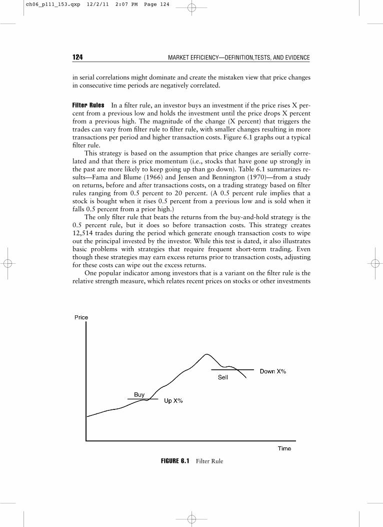
Filter Rules In a filter rule, an investor buys an investment if the price rises X per-cent from a previous low and holds the investment until the price drops X percentfrom a previous high. The magnitude of the change (X percent) that triggers thetrades can vary from filter rule to filter rule, with smaller changes resulting in moretransactions per period and higher transaction costs. Figure 6.1 graphs out a typicalfilter rule.

This strategy is based on the assumption that price changes are serially corre-lated and that there is price momentum (i.e., stocks that have gone up strongly inthe past are more likely to keep going up than go down). Table 6.1 summarizes re-sults—Fama and Blume (1966) and Jensen and Bennington (1970)—from a studyon returns, before and after transactions costs, on a trading strategy based on filterrules ranging from 0.5 percent to 20 percent. (A 0.5 percent rule implies that astock is bought when it rises 0.5 percent from a previous low and is sold when itfalls 0.5 percent from a prior high.)

The only filter rule that beats the returns from the buy-and-hold strategy is the0.5 percent rule, but it does so before transaction costs. This strategy creates12,514 trades during the period which generate enough transaction costs to wipeout the principal invested by the investor. While this test is dated, it also illustratesbasic problems with strategies that require frequent short-term trading. Eventhough these strategies may earn excess returns prior to transaction costs, adjustingfor these costs can wipe out the excess returns.

One popular indicator among investors that is a variant on the filter rule is therelative strength measure, which relates recent prices on stocks or other investments

124 MARKET EFFICIENCY—DEFINITION,TESTS, AND EVIDENCE

FIGURE 6.1 Filter Rule

ch06_p111_153.qxp 12/2/11 2:07 PM Page 124

to either average prices over a specified period, say over six months, or to the priceat the beginning of the period. Stocks that score high on the relative strength mea-sure are considered good investments. This investment strategy is also based uponthe assumption of price momentum.

Runs Tests A runs test is a nonparametric variation on the serial correlation,and it is based on a count of the number of runs (i.e., sequences of price in-creases or decreases) in the price changes. Thus, the following time series ofprice changes, where U is an increase and D is a decrease, would result in the fol-lowing runs:

UUU DD U DDD UU DD U D UU DD U DD UUU DD UU D UU D

There were 18 runs in this price series of 33 periods. The actual number of runsin the price series is compared against the number that can be expected in a se-ries of this length, assuming that price changes are random.9 If the actual num-ber of runs is greater than the expected number, there is evidence of negativecorrelation in price changes. If it is lower, there is evidence of positive correla-tion. A 1966 study by Niederhoffer and Osborne of price changes in the Dow 30stocks assuming daily, four-day, nine-day, and 16-day return intervals providedthe following results:

Time Series Properties of Price Changes 125

TABLE 6.1 Returns on Filter Rule Strategies

Return with Return with Number of Transactions Return afterValue of X Strategy Buy and Hold with Strategy Transaction Costs

0.5% 11.5% 10.4% 12,514 –103.6%1.0% 5.5% 10.3% 8,660 –74.9%2.0% 0.2% 10.3% 4,764 –45.2%3.0% –1.7% 10.1% 2,994 –30.5%4.0% 0.1% 10.1% 2,013 –19.5%5.0% –1.9% 10.0% 1,484 –16.6%6.0% 1.3% 9.7% 1,071 –9.4%7.0% 0.8% 9.6% 828 –7.4%8.0% 1.7% 9.6% 653 –5.0%9.0% 1.9% 9.6% 539 –3.6%

10.0% 3.0% 9.6% 435 –1.4%12.0% 5.3% 9.4% 289 2.3%14.0% 3.9% 10.3% 224 1.4%16.0% 4.2% 10.3% 172 2.3%18.0% 3.6% 10.0% 139 2.0%20.0% 4.3% 9.8% 110 3.0%

9There are statistical tables that summarize the expected number of runs, assuming random-ness, in a series of any length.

ch06_p111_153.qxp 12/2/11 2:07 PM Page 125

Differencing IntervalDaily Four-Day Nine-Day Sixteen-Day

Actual runs 735.1 175.7 74.6 41.6Expected runs 759.8 175.8 75.3 41.7

Based on these results, there is evidence of positive correlation in daily returns butno evidence of deviations from normality for longer return intervals.

Again, while the evidence is dated, it serves to illustrate the point that longstrings of positive and negative changes are, by themselves, insufficient evidencethat markets are not random, since such behavior is consistent with price changesfollowing a random walk. It is the recurrence of these strings that can be viewed asevidence against randomness in price behavior.

Long-Term Price Movements

While most of the earlier studies of price behavior focused on shorter return inter-vals, more attention has been paid to price movements over longer periods (one-year to five-year periods) in recent years. Here, there is an interesting dichotomy inthe results. When “long term” is defined as months rather than years, there seemsto be a tendency toward positive serial correlation or price momentum. However,when “long term” is defined in terms of years, there is substantial negative correla-tion in the returns, suggesting that markets reverse themselves over long periods.

Shorter-Term Price Momentum

In the last section, we noted that the evidence of short-term price patterns is weakand that any price dependence over very short time periods (minutes or hours)can be attributed more to market structure (liquidity, bid ask spreads) than to in-efficiency. We also argued that while chartists who track these short-term pricemovements abound, few seem to emerge as consistent winners. As we extend ourtime periods from minutes to days and from days to weeks, there is some evi-dence of price momentum. Put differently, stocks that have gone up in the lastfew weeks or months seem to have a tendency to continue to outperform the mar-ket in the next few weeks or months, and stocks that have gone down in the re-cent weeks or months continue to languish in the next few weeks or months.

Jegadeesh and Titman present evidence of what they call price momentum instock prices over time periods of up to eight months — stocks that have gone up in thelast six months tend to continue to go up, whereas stocks that have gone down in thelast six months tend to continue to go down. The momentum effect is just as strong inthe European markets, though it seems to be weaker in emerging markets. What maycause this momentum? One potential explanation is that mutual funds are more likelyto buy past winners and dump past losers, thus generating price continuity.

Longer-Term Price Reversal

When the long term is defined in terms of years, there is substantial negative correla-tion in returns, suggesting that markets reverse themselves over very long periods.Fama and French examined five-year returns on stocks from 1941 to 1985 and presentevidence of this phenomenon. They found that serial correlation is more negative in

126 MARKET EFFICIENCY—DEFINITION,TESTS, AND EVIDENCE

ch06_p111_153.qxp 12/2/11 2:07 PM Page 126

five-year returns than in one-year returns, and is much more negative for smallerstocks rather than larger stocks. Figure 6.2 summarizes one-year and five-years ser-ial correlation by size class for stocks on the New York Stock Exchange.

This phenomenon has also been examined in other markets, and the findings havebeen similar. There is evidence that returns reverse themselves over long time periods.

Since there is evidence that prices reverse themselves in the long term for entiremarkets, it might be worth examining whether such price reversals occur on classes ofstock within a market. For instance, are stocks that have gone up the most over the lastperiod more likely to go down over the next period and vice versa? To isolate the effectof such price reversals on the extreme portfolios, DeBondt and Thaler constructed awinner portfolio of 35 stocks, which had gone up the most over the prior year, and aloser portfolio of 35 stocks, which had gone down the most over the prior year, eachyear from 1933 to 1978, and examined returns on these portfolios for the sixty monthsfollowing the creation of the portfolio. Figure 6.3 summarizes the excess returns forwinner and loser portfolios . This analysis suggests that loser portfolios clearly outper-form winner portfolios in the 60 months following creation. This evidence is consistentwith market overreaction and correction in long return intervals.

There are many, academics as well as practitioners, who suggest that thesefindings may be interesting but that they overstate potential returns on loserportfolios. For instance, there is evidence that loser portfolios are more likely tocontain low-priced stocks (selling for less than $5), which generate higher trans-actions costs and are also more likely to offer heavily skewed returns; that is, theexcess returns come from a few stocks making phenomenal returns rather thanfrom consistent performance. One study of the winner and loser portfolios at-tributes the bulk of the excess returns of loser portfolios to low-priced stocksand also finds that the results are sensitive to when the portfolios are created.

Time Series Properties of Price Changes 127

FIGURE 6.2 One-Year and Five-Year Correlations: Market Value Class: 1941–1985Source: Fama and French (1988).

Smallest 2 3 4 5 6 7 8 9 Largest

1 Year5 Year

−0.60

−0.50

−0.40

−0.30

−0.20

−0.10

0.00

Cor

rela

tion

in R

etur

ns

Market Value Class

ch06_p111_153.qxp 12/2/11 2:07 PM Page 127

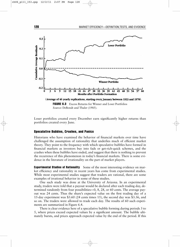
Loser portfolios created every December earn significantly higher returns thanportfolios created every June.

Speculative Bubbles, Crashes, and Panics

Historians who have examined the behavior of financial markets over time havechallenged the assumption of rationality that underlies much of efficient markettheory. They point to the frequency with which speculative bubbles have formed infinancial markets as investors buy into fads or get-rich-quick schemes, and thecrashes when these bubbles have ended, and suggest that there is nothing to preventthe recurrence of this phenomenon in today’s financial markets. There is some evi-dence in the literature of irrationality on the part of market players.

Experimental Studies of Rationality Some of the most interesting evidence on mar-ket efficiency and rationality in recent years has come from experimental studies.While most experimental studies suggest that traders are rational, there are someexamples of irrational behavior in some of these studies.

One such study was done at the University of Arizona. In an experimentalstudy, traders were told that a payout would be declared after each trading day, de-termined randomly from four possibilities—0, 8, 28, or 60 cents. The average pay-out was 24 cents. Thus the share’s expected value on the first trading day of a15-day experiment was $3.60 (24 cents times 15), the second day was $3.36, andso on. The traders were allowed to trade each day. The results of 60 such experi-ments are summarized in Figure 6.4.

There is clear evidence here of a speculative bubble forming during periods 3 to5, where prices exceed expected values by a significant amount. The bubble ulti-mately bursts, and prices approach expected value by the end of the period. If this

FIGURE 6.3 Excess Returns for Winner and Loser PortfoliosSource: DeBondt and Thaler (1985).

128 MARKET EFFICIENCY—DEFINITION,TESTS, AND EVIDENCE

ch06_p111_153.qxp 12/2/11 2:07 PM Page 128

mispricing is feasible in a simple market, where every investor obtains the sameinformation, it is clearly feasible in real financial markets, where there is muchmore differential information and much greater uncertainty about expected value.

It should be pointed out that some of the experiments were run with students,and some with Tucson businessmen with real-world experience. The results weresimilar for both groups. Furthermore, when price curbs of 15 cents were intro-duced, the booms lasted even longer because traders knew that prices would notfall by more than 15 cents in a period. Thus, the notion that price limits can controlspeculative bubbles seems misguided.

Behavioral Finance The irrationality sometimes exhibited by investors has givenrise to a whole new area of finance called behavioral finance. Using evidence gath-ered from experimental psychology, researchers have tried to both model how in-vestors react to information and predict how prices will change as a consequence.They have been far more successful at the first endeavor than the second. For in-stance, the evidence seems to suggest that:

■ Investors do not like to admit their mistakes. Consequently, they tend to holdon to losing stocks far too long, or in some cases double up their bets (invest-ments) as stocks drop in value.

■ More information does not always lead to better investment decisions. In-vestors seem to suffer both from information overload and from a tendency toreact to the latest piece of information. Both result in investment decisions thatlower returns in the long term.

If the evidence on how investors behave is so clear-cut, you might ask, why arethe predictions that emerge from these models so noisy? The answer, perhaps, isthat any model that tries to forecast human foibles and irrationalities is, by its verynature, unlikely to be a stable one. Behavioral finance may emerge ultimately as a

FIGURE 6.4 Trading Price by Trading Day

Time Series Properties of Price Changes 129

ch06_p111_153.qxp 12/2/11 2:07 PM Page 129

trump card in explaining why and how stock prices deviate from true value, but itsrole in devising investment strategy still remains questionable.

MARKET REACTION TO INFORMATION EVENTS

Some of the most powerful tests of market efficiency are event studies where mar-ket reaction to informational events (such as earnings and takeover announce-ments) has been scrutinized for evidence of inefficiency. While it is consistent withmarket efficiency for markets to react to new information, the reaction has to be in-stantaneous and unbiased. This point is made in Figure 6.5 by contrasting three dif-ferent market reactions to information announcements.

BEHAVORIAL FINANCE AND VALUATION

In 1999, Robert Shiller made waves in both academia and investment houseswith his book titled Irrational Exuberance. His thesis is that investors are of-ten not just irrational but irrational in predictable ways—overreacting tosome information and buying and selling in herds. His work forms part of agrowing body of theory and evidence of behavioral finance, which can beviewed as a congruence of psychology, statistics, and finance.

While the evidence presented for investor irrationality is strong, the impli-cations for valuation are less so. You can consider discounted cash flow valua-tion to be the antithesis of behavioral finance, because it takes the point ofview that the value of an asset is the present value of the expected cash flowsgenerated by that asset. With this context, there are two ways in which youcan look at the findings in behavioral finance:

1. Irrational behavior may explain why prices can deviate from value (as es-timated in a discounted cash flow model). Consequently, it provides thefoundation for the excess returns earned by rational investors who basedecisions on estimated value. Implicit here is the assumption that marketsultimately recognize their irrationality and correct themselves.

2. It may also explain why discounted cash flow values can deviate from rel-ative values (estimated using multiples). Since the relative value is esti-mated by looking at how the market prices similar assets, irrationalitiesthat exist will be priced into the asset.

130 MARKET EFFICIENCY—DEFINITION,TESTS, AND EVIDENCE

FIGURE 6.5 Information and Price Adjustment

ch06_p111_153.qxp 12/2/11 2:07 PM Page 130

Of the three market reactions pictured here, only the first one is consistentwith an efficient market. In the second market, the information announcement isfollowed by a gradual increase in prices, allowing investors to make excess re-turns after the announcement. This is a slow learning market where some in-vestors will make excess returns on the price drift. In the third market, the pricereacts instantaneously to the announcement, but corrects itself in the days thatfollow, suggesting that the initial price change was an overreaction to the infor-mation. Here again, an enterprising investor could have sold short after the an-nouncement and expected to make excess returns as a consequence of the pricecorrection.

Earnings Announcements

When firms make earnings announcements, they convey information to financialmarkets about their current and future prospects. The magnitude of the informa-tion, and the size of the market reaction, should depend on how much the earningsreport exceeds or falls short of investor expectations. In an efficient market, thereshould be an instantaneous reaction to the earnings report, if it contains surprisinginformation, and prices should increase following positive surprises and decline fol-lowing negative surprises.

Since actual earnings are compared to investor expectations, one of the key partsof an earnings event study is the measurement of these expectations. Some of the ear-lier studies used earnings from the same quarter in the prior year as a measure of ex-pected earnings (i.e., firms that report increases in quarter-to-quarter earnings providepositive surprises, and those which report decreases in quarter-to-quarter earningsprovide negative surprises). In more recent studies, analyst estimates of earnings havebeen used as a proxy for expected earnings and compared to the actual earnings.

Figure 6.6 provides a graph of price reactions to earnings surprises, classifiedon the basis of magnitude into different classes from “most negative” earnings re-ports (group 1) to “most positive” earnings reports (group 10). The evidence con-tained in this graph is consistent with the evidence in most earnings announcementstudies:

■ The earnings announcement clearly conveys valuable information to financialmarkets; there are positive excess returns (cumulative abnormal returns) afterpositive announcements and negative excess returns around negative an-nouncements.

■ There is some evidence of a market reaction in the day immediately prior to theearnings announcement that is consistent with the nature of the announcement(i.e., prices tend to go up on the day before positive announcements and down onthe day before negative announcements). This can be viewed as evidence of eitherinsider trading, information leakage, or getting the announcement date wrong.10

10The Wall Street Journal is often used as an information source to extract announcementdates for earnings. For some firms, news of the announcement may actually cross the newswire the day before the Wall Street Journal announcement, leading to a misidentification ofthe report date and the drift in returns the day before the announcement.

Market Reaction to Information Events 131

ch06_p111_153.qxp 12/2/11 2:07 PM Page 131

■ There is some evidence, albeit weak, of a price drift in the days following anearnings announcement. Thus a positive report evokes a positive market reac-tion on the announcement date, and there are mildly positive excess returns inthe days following the earnings announcement. Similar conclusions emerge fornegative earnings reports.

The management of a firm has some discretion on the timing of earnings re-ports, and there is some evidence that the timing affects expected returns. A 1989study by Damodaran of earnings reports, classified by the day of the week that theearnings are reported, reveals that earnings and dividend reports on Fridays aremuch more likely to contain negative information than announcements on anyother day of the week. This is shown in Figure 6.7.

There is also some evidence discussed by Chamber and Penman (1984) thatearnings announcements that are delayed, relative to the expected announcementdate, are much more likely to contain bad news than earnings announcements

FIGURE 6.6 Price Reaction to Quarterly Earnings ReportSource: Rendleman, Jones, and Latrané (1982).

132 MARKET EFFICIENCY—DEFINITION,TESTS, AND EVIDENCE

ch06_p111_153.qxp 12/2/11 2:07 PM Page 132

that are early or on time. This is graphed in Figure 6.8. Earnings announcementsthat are more than six days late relative to the expected announcement date aremuch more likely to contain bad news and evoke negative market reactions thanearnings announcements that are on time or early.

Investment and Project Announcements

Firms frequently make announcements of their intentions of investing resourcesin projects and research and development. There is evidence that financial mar-kets react to these announcements. The question of whether markets have a long-term or short-term perspective can be partially answered by looking at thesemarket reactions. If financial markets are as short-term as some of their criticsclaim, they should react negatively to announcements by the firm that it plans toinvest in research and development. The evidence suggests the contrary. Table 6.2summarizes market reactions to various classes of investment announcementsmade by the firm.

This table excludes the largest investments that most firms make, which is ac-quisitions of other firms. Here the evidence is not so favorable. In about 55 per-cent of all acquisitions, the stock price of the acquiring firm drops on theannouncement of the acquisition, reflecting the market’s beliefs that firms tend tooverpay on acquisitions.

FIGURE 6.7 Earnings and Dividend Reports by Day of the WeekSource: Damodaran (1989).

–6.00%

–4.00%

–2.00%

0.00%

2.00%

4.00%

6.00%

8.00%

Monday Tuesday Wednesday Thursday Friday

% Change (EPS) % Change (DPS)

Ear

ning

s Div

iden

ds

Exc

ess

Ret

urns

Market Reaction to Information Events 133

ch06_p111_153.qxp 12/2/11 2:07 PM Page 133

MARKET ANOMALIES

Merriam-Webster’s Collegiate Dictionary defines an anomaly as a “deviation fromthe common rule.” Studies of market efficiency have uncovered numerous exam-ples of market behavior that are inconsistent with existing models of risk and re-turn and often defy rational explanation. The persistence of some of these patternsof behavior suggests that the problem, in at least some of these anomalies, lies inthe models being used for risk and return rather than in the behavior of financialmarkets. The following section summarizes some of the more widely noticed anom-alies in financial markets in the United States and elsewhere.

Anomalies Based on Firm Characteristics

There are a number of anomalies that have been related to observable firm charac-teristics, including the market value of equity, price-earnings ratios, and price–bookvalue ratios.

134 MARKET EFFICIENCY—DEFINITION,TESTS, AND EVIDENCE

FIGURE 6.8 Cumulated Abnormal Returns and Earnings DelaySource: Chambers and Penman (1984).

Day 0 Is Earnings Announcement Date0.006

–0.014

0 +30–30

Delay > 6 days

Early > 6 days

Cum

ulat

ive

Abn

orm

al R

etur

n

TABLE 6.2 Market Reactions to Investment Announcements

Abnormal Returns

On InType of Announcement Announcement Day Announcement Month

Joint venture formations 0.399% 1.412%R&D expenditures 0.251% 1.456%Product strategies 0.440% –0.35%Capital expenditures 0.290% 1.499%All announcements 0.355% 0.984%

Source: Chan, Martin, and Kensinger (1990); McConnell and Muscarella (1985).

ch06_p111_153.qxp 12/2/11 2:07 PM Page 134

The Small Firm Effect Studies such as Banz (1981) and Keim (1983) have consis-tently found that smaller firms (in terms of market value of equity) earn higher re-turns than larger firms of equivalent risk, where risk is defined in terms of themarket beta. Figure 6.9 summarizes returns for stocks in 10 market value classesfor the period from 1927 to 1983.

The size of the small firm premium, while it has varied across time, has beengenerally positive. It was highest during the 1970s and early 1980s and lowestduring the 1990s. The persistence of this premium has led to several possibleexplanations.

1. The transaction costs of investing in small stocks are significantly higherthan the transaction costs of investing in larger stocks, and the premiums are esti-mated prior to these costs. While this is generally true, the differential transactioncosts are unlikely to explain the magnitude of the premium across time, and arelikely to become even less critical for longer investment horizons. The difficulties ofreplicating the small firm premiums that are observed in the studies in real time areillustrated in Figure 6.10, which compares the returns on a hypothetical small firmportfolio (CRSP Small Stocks) with the actual returns on a small firm mutual fund(DFA Small Stock Fund), which passively invests in small stocks.

2. The capital asset pricing model may not be the right model for risk, andbetas underestimate the true risk of small stocks. Thus, the small firm premiumis really a measure of the failure of beta to capture risk. The additional risk as-sociated with small stocks may come from several sources. First, the estimationrisk associated with estimates of beta for small firms is much greater than theestimation risk associated with beta estimates for larger firms. The small firmpremium may be a reward for this additional estimation risk. Second, there maybe additional risk in investing in small stocks because far less information is

Market Anomalies 135

FIGURE 6.9 Annual Returns by Size Class, 1927–1983

Smallest 3 5 7 9

Size Class

0.00%

2.00%

4.00%

6.00%

8.00%

10.00%

12.00%

14.00%

16.00%

18.00%

20.00%

ch06_p111_153.qxp 12/2/11 2:07 PM Page 135

 

available on these stocks. In fact, studies indicate that stocks that are neglectedby analysts and institutional investors earn an excess return that parallels thesmall firm premium.

There is evidence of a small firm premium in markets outside the United States aswell. Dimson and Marsh (1986) examined stocks in the United Kingdom from 1955 to1984 and found that the annual returns on small stocks exceeded that on large stocksby 6 percent annually over the period. Chan, Hamao, and Lakonishok (1991) report asmall firm premium of about 5 percent for Japanese stocks between 1971 and 1988.

Price-Earnings Ratios Investors have long argued that stocks with low price-earn-ings ratios are more likely to be undervalued and earn excess returns. For instance,Benjamin Graham, in his investment classic The Intelligent Investor, used lowprice-earnings ratios as a screen for finding undervalued stocks. Studies [Basu(1977); Basu (1983)] that have looked at the relationship between PE ratios and ex-cess returns confirm these priors. Figure 6.11 summarizes annual returns by PE ra-tio classes for stocks from 1967 to 1988. Firms in the lowest PE ratio class earnedan average return of 16.26 percent during the period, while firms in the highest PEratio class earned an average return of only 6.64 percent.

The excess returns earned by low PE ratio stocks also persist in other interna-tional markets. Table 6.3 summarizes the results of studies looking at this phenom-enon in markets outside the United States.

The excess returns earned by low price-earnings ratio stocks are difficult to jus-tify using a variation of the argument used for small stocks (i.e., that the risk of lowPE ratios stocks is understated in the CAPM). Low PE ratio stocks generally arecharacterized by low growth, large size, and stable businesses, all of which shouldwork toward reducing their risk rather than increasing it. The only explanationthat can be given for this phenomenon, which is consistent with an efficient market,is that low PE ratio stocks generate large dividend yields, which would have createda larger tax burden because dividends are taxed at higher rates.

136 MARKET EFFICIENCY—DEFINITION,TESTS, AND EVIDENCE

FIGURE 6.10 Returns on CRSP Small Stocks versus DFA Small Stock Fund

–10.00%

–5.00%

0.00%

5.00%

10.00%

15.00%

1982 1983 1984 1985 1986 1987 1988 1989 1990 1991

CRSP Small Stocks DFA Small Stock Fund

ch06_p111_153.qxp 12/2/11 2:07 PM Page 136

Price–Book Value Ratios Another statistic that is widely used by investors in invest-ment strategy is price–book value ratios. A low price–book value ratio has been con-sidered a reliable indicator of undervaluation in firms. In studies that parallel thosedone on price-earnings ratios, the relationship between returns and price–book valueratios has been studied. The consistent finding from these studies is that there is anegative relationship between returns and price–book value ratios—low price–bookvalue ratio stocks earn higher returns than high price–book value ratio stocks.

Market Anomalies 137

FIGURE 6.11 Annual Returns by PE Ratio Class

0.00%

2.00%

4.00%

6.00%

8.00%

10.00%

12.00%

14.00%

16.00%

18.00%

Lowest 3 5 7 9

TABLE 6.3 Excess Returns on Low PE Ratio Stocks by Country,1989–1994

Annual Premium Earned byCountry Lowest-PE Stocks (Bottom Quintile)

Australia 3.03%France 6.40%Germany 1.06%Hong Kong 6.60%Italy 14.16%Japan 7.30%Switzerland 9.02%United Kingdom 2.40%

Annual premium: Premium earned over an index of equallyweighted stocks in that market between January 1, 1989, andDecember 31, 1994. These numbers were obtained from a Mer-rill Lynch Survey of Proprietary Indices.

ch06_p111_153.qxp 12/2/11 2:07 PM Page 137

 

Rosenberg, Reid, and Lanstein (1985) find that the average returns on U.S.stocks are positively related to the ratio of a firm’s book value to market value. Be-tween 1973 and 1984, the strategy of picking stocks with high book-price ratios(low price-book values) yielded an excess return of 36 basis points a month. Famaand French (1992), in examining the cross section of expected stock returns be-tween 1963 and 1990, established that the positive relationship between book-to-price ratios and average returns persists in both the univariate and multivariatetests, and is even stronger than the size effect in explaining returns. When they clas-sified firms on the basis of book-to-price ratios into 12 portfolios, firms in the low-est book-to-price (highest price-book) class earned an average monthly return of0.30 percent, while firms in the highest book-to-price (lowest price-book) classearned an average monthly return of 1.83 percent for the 1963–1990 period.

Chan, Hamao, and Lakonishok (1991) find that the book-to-market ratio hasa strong role in explaining the cross section of average returns on Japanese stocks.Capaul, Rowley, and Sharpe (1993) extend the analysis of price–book value ratiosacross other international markets, and conclude that value stocks (i.e., stockswith low price–book value ratios) earned excess returns in every market thatthey analyzed between 1981 and 1992. Their annualized estimates of the returndifferential earned by stocks with low price–book value ratios, over the marketindex, were:

Added Return to Low Country Price–Book Value Portfolio

France 3.26%Germany 1.39%Switzerland 1.17%United Kingdom 1.09%Japan 3.43%United States 1.06%Europe 1.30%Global 1.88%

A caveat is in order. Fama and French pointed out that low price–book valueratios may operate as a measure of risk, since firms with prices well below bookvalue are more likely to be in trouble and go out of business. Investors thereforehave to evaluate for themselves whether the additional returns made by such firmsjustify the additional risk taken on by investing in them.

Temporal Anomalies

There are a number of peculiarities in return differences across calendar time thatnot only are difficult to rationalize but are also suggestive of inefficiencies. Further-more, some of these temporal anomalies are related to the small firm effect de-scribed in the previous section.

January Effect Studies of returns in the United States and other major financialmarkets [Roll (1983); Haugen and Lakonishok (1988)] consistently reveal strongdifferences in return behavior across the months of the year. Figure 6.12 reportsaverage returns by months of the year from 1926 to 1983. Returns in January are

138 MARKET EFFICIENCY—DEFINITION,TESTS, AND EVIDENCE

ch06_p111_153.qxp 12/2/11 2:07 PM Page 138

significantly higher than returns in any other month of the year. This phenomenonis called the year-end or January effect, and it can be traced to the first two weeks inJanuary.

The relationship between the January effect and the small firm effect [(Keum(1983) and Reinganum (1983)] adds to the complexity of this phenomenon. TheJanuary effect is much more accentuated for small firms than for larger firms, androughly half of the small firm premium described in the prior section is earned inthe first two weeks of January. Figure 6.13 graphs returns in January by size andrisk class for data from 1935 to 1986.

A number of explanations have been advanced for the January effect, but fewhold up to serious scrutiny. Reinganum suggested that there is tax loss selling byinvestors at the end of the year on stocks that have lost money to capture the cap-ital gain, driving prices down, presumably below true value, in December, and abuying back of the same stocks in January,11 resulting in the high returns. The factthat the January effect is accentuated for stocks that have done worse over theprior year is offered as evidence for this explanation. There are several pieces ofevidence that contradict it, though. First, there are countries, like Australia, thathave a different tax year but continue to have a January effect. Second, the Janu-ary effect is no greater, on average, in years following bad years for the stock mar-ket than in other years.

A second rationale is that the January effect is related to institutional tradingbehavior around the turn of the years. It has been noted, for instance, that the ratioof buys to sells for institutions drops significantly below average in the days before

Market Anomalies 139

FIGURE 6.12 Average Return by Months of the Year, 1926–1983

–2.00%

–1.00%

0.00%

1.00%

2.00%

3.00%

4.00%

5.00%

Janu

ary

Febr

uary

Mar

ch

Apr

il

May

June

July

Aug

ust

Sep

tem

ber

Oct

ober

Nov

embe

r

Dec

embe

r

Ave

rage

Mon

thly

Ret

urn

11Since wash sales rules would prevent an investor from selling and buying back the samestock within 45 days, there has to be some substitution among the stocks. Thus investor 1sells stock A and investor 2 sells stock B, but when it comes time to buy back the stock, in-vestor 1 buys stock B and investor 2 buys stock A.

ch06_p111_153.qxp 12/2/11 2:07 PM Page 139

 

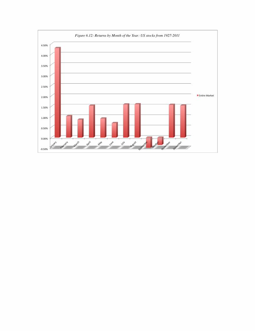
the turn of the year and picks up to above average in the months that follow. This isillustrated in Figure 6.14. It is argued that the absence of institutional buyingpushes down prices in the days before the turn of the year and pushes up prices inthe days after.

The universality of the January effect is illustrated in Figure 6.15, which exam-ines returns in January versus the other months of the year in several major finan-cial markets, and finds strong evidence of a January effect in every market [Haugenand Lakonishok (1988); Gultekin and Gultekin (1983)].

Weekend Effect The weekend effect is another return phenomenon that has persistedover extraordinarily long periods and over a number of international markets. It refersto the differences in returns between Mondays and other days of the week. The signifi-cance of the return difference is brought out in Figure 6.16, which graphs returns bydays of the week from 1962 to 1978 [Gibbons and Hess (1981)].

The returns on Mondays are significantly negative, whereas the returns onevery day of the week are not. There are a number of other findings on the Mondayeffect that have fleshed this out. First, the Monday effect is really a weekend effectsince the bulk of the negative returns is manifested in the Friday close to Mondayopen returns. The intraday returns on Monday are not the culprits in creating the

140 MARKET EFFICIENCY—DEFINITION,TESTS, AND EVIDENCE

FIGURE 6.13 Returns in January by Size and Risk Class, 1935–1986Source: Ritter and Chopra (1989).

ch06_p111_153.qxp 12/2/11 2:07 PM Page 140

negative returns. Second, the Monday effect is worse for small stocks than forlarger stocks. Third, the Monday effect is no worse following three-day weekendsthan following two-day weekends.

There are some who have argued that the weekend effect is the result of badnews being revealed after the close of trading on Friday and during the weekend.They point to Figure 6.7, which reveals that more negative earnings reports are re-vealed after close of trading on Friday. Even if this were a widespread phenomenon,the return behavior would be inconsistent with a rational market, since rational in-vestors would build the expectation of the bad news over the weekend into theprice before the weekend, leading to an elimination of the weekend effect.

The weekend effect is fairly strong in most major international markets, asshown in Figure 6.17. The presence of a strong weekend effect in Japan, which al-lowed Saturday trading for a portion of the period studied here, indicates that theremight be a more direct reason for negative returns on Mondays than bad informa-tion over the weekend.

As a final note, the negative returns on Mondays cannot be attributed to justthe absence of trading over the weekend. The returns on days following tradingholidays in general are characterized by positive, not negative, returns. Figure 6.18summarizes returns on trading days following major holidays and confirms thispattern.

Market Anomalies 141

FIGURE 6.14 Institutional Buying/ Selling around Year-End

ch06_p111_153.qxp 12/2/11 2:07 PM Page 141

EVIDENCE ON INSIDERS AND INVESTMENT PROFESSIONALS

There is a sense that insiders, analysts, and portfolio managers must possess an ad-vantage over the average investors in the market and be able to convert this advan-tage into excess returns. The evidence on the performance of these investors isactually surprisingly mixed.

Insider Trading

The Securities and Exchange Commission (SEC) defines an insider to be an officer ordirector of the firm or a major stockholder (holding more than 5 percent of the out-standing stock in the firm). Insiders are barred from trading in advance of specific in-formation on the company and are required to file with the SEC when they buy orsell stock in the company. If it is assumed, as seems reasonable, that insiders have bet-ter information about the company and consequently better estimates of value thanother investors, the decisions by insiders to buy and sell stock should affect stock

FIGURE 6.15 Returns in January versus Other Months—Major Financial MarketsSource: Gultekin and Gultekin (1983).

142 MARKET EFFICIENCY—DEFINITION,TESTS, AND EVIDENCE

ch06_p111_153.qxp 12/2/11 2:07 PM Page 142

FIGURE 6.16 Average Daily Returns by Day of the Week, 1962–1978Source: Gibbons and Hess (1981).

–0.15%

–0.10%

–0.05%

0.00%

0.05%

0.10%

0.15%

Monday Tuesday Wednesday Thursday Friday

Ave

rage

Dai

ly R

etur

n

FIGURE 6.17 Weekend Effect in International Markets

–0.20%

–0.10%

0.00%

0.10%

0.20%

0.30%

0.40%

Aus

tral

ia

Hon

gK

ong

Can

ada

Japa

n

Fran

ce

Mal

aysi

a

Phi

lipp

ines

Sin

gapo

re

Uni

ted

Kin

gdom

Uni

ted

Sta

tes

Monday Rest of the Week

Evidence on Insiders and Investment Professionals 143

ch06_p111_153.qxp 12/2/11 2:07 PM Page 143

prices. Figure 6.19, derived from an early study of insider trading by Jaffe (1974), ex-amines excess returns on two groups of stock, classified on the basis of insider trades.The “buy group” includes stocks where buys exceeded sells by the biggest margin,and the “sell group” includes stocks where sells exceed buys by the biggest margin.

While it seems like the buy group does significantly better than the sell groupin this study, advances in information technology have made this information oninsider trading available to more and more investors. A more recent study [Sey-hun (1998)] of insider trading examined excess returns around both the date theinsiders report to the SEC and the date that information becomes available to in-vestors in the official summary. Figure 6.20 presents the contrast between the twoevent dates.

144 MARKET EFFICIENCY—DEFINITION,TESTS, AND EVIDENCE

FIGURE 6.18 A Holiday Effect? Average Market Returns on Holidays

New Year's Day

President's Day

Good Friday

Memorial Day

Fourth of July

Labor Day

Thanksgiving

Christmas

Average of All Days

–0.05% 0.00% 0.05% 0.10% 0.15% 0.20% 0.25% 0.30% 0.35% 0.40%

FIGURE 6.19 Cumulative Returns Following Insider Trading: Buy versus Sell GroupSource: Jaffe (1974).

–0.05

0

0.050.1

0.15

0.2

0.250.3

0.35

0.4

1 2 3 4 5 6 7 8 9 10 11 12 13 14 15 16 17 18 19 20

Month Following Insider Trade

Buy Group-M Sell Group-M

ch06_p111_153.qxp 12/2/11 2:07 PM Page 144

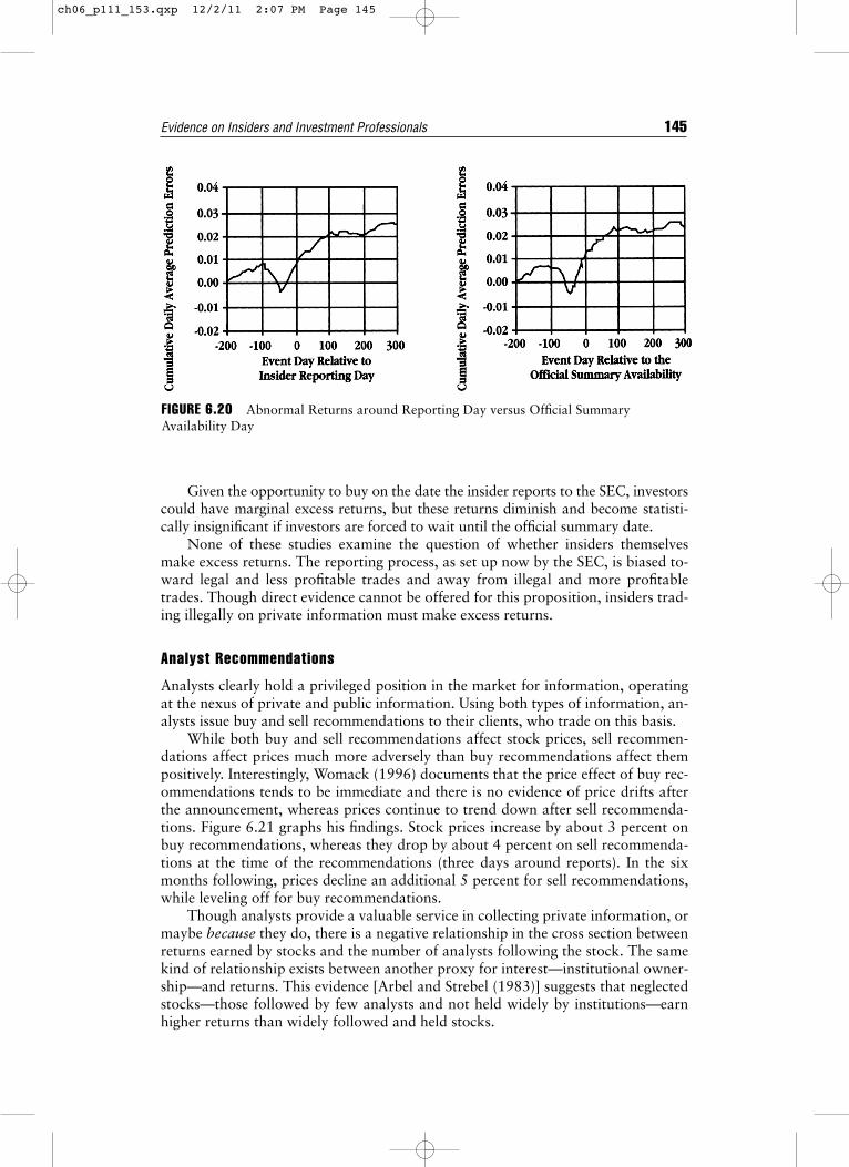
Given the opportunity to buy on the date the insider reports to the SEC, investorscould have marginal excess returns, but these returns diminish and become statisti-cally insignificant if investors are forced to wait until the official summary date.

None of these studies examine the question of whether insiders themselvesmake excess returns. The reporting process, as set up now by the SEC, is biased to-ward legal and less profitable trades and away from illegal and more profitabletrades. Though direct evidence cannot be offered for this proposition, insiders trad-ing illegally on private information must make excess returns.

Analyst Recommendations

Analysts clearly hold a privileged position in the market for information, operatingat the nexus of private and public information. Using both types of information, an-alysts issue buy and sell recommendations to their clients, who trade on this basis.

While both buy and sell recommendations affect stock prices, sell recommen-dations affect prices much more adversely than buy recommendations affect thempositively. Interestingly, Womack (1996) documents that the price effect of buy rec-ommendations tends to be immediate and there is no evidence of price drifts afterthe announcement, whereas prices continue to trend down after sell recommenda-tions. Figure 6.21 graphs his findings. Stock prices increase by about 3 percent onbuy recommendations, whereas they drop by about 4 percent on sell recommenda-tions at the time of the recommendations (three days around reports). In the sixmonths following, prices decline an additional 5 percent for sell recommendations,while leveling off for buy recommendations.

Though analysts provide a valuable service in collecting private information, ormaybe because they do, there is a negative relationship in the cross section betweenreturns earned by stocks and the number of analysts following the stock. The samekind of relationship exists between another proxy for interest—institutional owner-ship—and returns. This evidence [Arbel and Strebel (1983)] suggests that neglectedstocks—those followed by few analysts and not held widely by institutions—earnhigher returns than widely followed and held stocks.

Evidence on Insiders and Investment Professionals 145

FIGURE 6.20 Abnormal Returns around Reporting Day versus Official SummaryAvailability Day

ch06_p111_153.qxp 12/2/11 2:07 PM Page 145

Money Managers

Professional money managers operate as the experts in the field of investments.They are supposed to be better informed, have lower transaction costs, and bebetter investors overall than smaller investors. The earliest study of mutual fundsby Jensen (1968) suggested that this supposition might not hold in practice. Hisfindings, summarized in Figure 6.22 as excess returns on mutual funds, were thatthe average portfolio manager actually underperformed the market between 1955and 1964.

These results have been replicated with mild variations in their conclusions.In the studies that are most favorable for professional money managers, theybreak even against the market after adjusting for transaction costs, and in thosethat are least favorable they underpeform the market even before adjusting fortransaction costs.

The results, when categorized on a number of different bases, do not offermuch solace. For instance, Figure 6.23 shows excess returns from 1983 to 1990and the percentage of money managers beating the market, categorized by invest-ment style. Money managers in every investment style underperform the marketindex.

Figure 6.24 looks at the payoff to active portfolio management by measuringthe added value from trading actively during the course of the year, and finds thatreturns drop between 0.5 percent and 1.5 percent a year as a consequence.

146 MARKET EFFICIENCY—DEFINITION,TESTS, AND EVIDENCE

FIGURE 6.21 Market Reaction to Recommendations, 1989–1990Source: Womack (1996).

Removed from Sell

Added to SellRemoved from Buy

Added to BuyRet

urns

10.00%

8.00%

6.00%

4.00%

2.00%

0.00%

–2.00%

–4.00%

–6.00%

–8.00%

–10.00%

3 days around recommendation 1 month after 3 months after 6 months after

ch06_p111_153.qxp 12/2/11 2:07 PM Page 146

Finally, we find no evidence of continuity in performance. It classified moneymanagers into quartiles and examined the probabilities of movement from onequartile to another each year from 1983 to 1990. The results are summarized inTable 6.4.

Evidence on Insiders and Investment Professionals 147

FIGURE 6.23 Performance of Equity Funds, 1983–1990

Growth Yield Value Other All Funds S&P 5000%

10%

20%

30%

40%

50%

60%

Annual Return

% Underperforming Index

FIGURE 6.22 Mutual Fund Performance, 1955–1964—the Jensen StudySource: Jensen (1968).

–0.08 –0.06 –0.04 –0.02 0 0.02 0.04 0.06

Intercept [Actual Return—E(R)]

ch06_p111_153.qxp 12/2/11 2:07 PM Page 147

Table 6.4 indicates that a money manager who was ranked in the first quar-tile in a period had a 26 percent chance of being ranked in the first quartile in thenext period and a 27 percent chance of being ranked in the bottom quartile.There is some evidence of reversal in the portfolio managers in the lowest quar-tile, though some of that may be a reflection of the higher-risk portfolios that theyput together.

Thus, the overall evidence is that money managers collectively add littlevalue for investors with their active investing strategies. So, is there any goodnews for money managers in these studies? There are some glimmers:

■ Hot hands phenomenon: While there is little evidence of overall continuing inmutual fund performance, there is some evidence that money managers whohave performed well in the recent past are likely to outperform the market inthe near future. It is unclear, however, how long this momentum lasts, before

148 MARKET EFFICIENCY—DEFINITION,TESTS, AND EVIDENCE

FIGURE 6.24 The Payoff to Active Money Management: Equity FundsNote: This chart measures the difference between actual return on equity funds and returnon hypothetical portfolio frozen at beginning of period.

Growth Yield Value Other All

–1.60%

–1.40%

–1.20%

–1.00%

–0.80%

–0.60%

–0.40%

–0.20%

0.00%

TABLE 6.4 Probabilities of Transition from One Quartile to Another

Ranking Next Period

Ranking This Period 1 2 3 4

1 26% 24% 23% 27%2 20% 26% 29% 25%3 22% 28% 26% 24%4 32% 22% 22% 24%

ch06_p111_153.qxp 12/2/11 2:07 PM Page 148

there is reversal. This evidence mirrors our earlier analysis of stock pricesshowing momentum over weeks and months and reversing themselves in thelong term. Even this good news has to be taken with an ounce of caution,since it is possible that sheer chance and selection bias can still explain thesepositive runs of superior performance.

■ Skill versus luck: There is some debate as to whether the differences in re-turns that money managers earn over long periods can be entirely attributedto luck. Fama and French (2010) argue that when returns are measured net ofcosts, there is little evidence that mutual funds beat the market. However,when they look at gross returns, there is some evidence of differences in skill;they estimate that superior managers generate about 1.25% more than theaverage.

■ Tax, liquidity, and time horizon arbitrage: A money manager with a tax ratemuch lower than that of other money managers, lower need for liquidity orlower transactions costs than other investors, and/or a longer time horizonmay be able to exploit these differences to get investments at bargain pricesand earn excess returns. Although there is anecdotal evidence that such in-vestors exist, many of them are undone by their own success; as they attractmore money, they lose their focus and their competitive edge.

The bottom line: It is possible to beat the market, but it is hard work. Thereare no magic bullets or simple formulae for investment success. The money man-agers who beat the market consistently over time tend to be few and far between.Although they may adopt different strategies and have different views on mar-kets, they share some common characteristics. They have well thought out invest-ment philosophies, play to their strengths, and stay disciplined.

CONCLUSION

The question of whether markets are efficient will always be a provocative one,given the implications that efficient markets have for investment management andresearch. If an efficient market is defined as one where the market price is an unbi-ased estimate of the true value, it is quite clear that some markets will always bemore efficient than others and that markets will always be more efficient to someinvestors than to others. The capacity of a market to correct inefficiencies quicklywill depend, in part, on the ease of trading, the transaction costs, and the vigilanceof profit-seeking investors in that market.

While market efficiency can be tested in a number of different ways, the twomost widely used tests to test efficiency are event studies, which examine market re-actions to information events, and portfolio studies, which evaluate the returns ofportfolios created on the basis of observable characteristics. It does make sense tobe vigilant, because bias can enter these studies, intentionally or otherwise, in anumber of different ways and can lead to unwarranted conclusions and, worse still,wasteful investment strategies.

There is substantial evidence of irregularities in market behavior related tosystematic factors such as size, price-earnings ratios, and price–book value ratios,as well as to time—the January and the weekend effects. While these irregularitiesmay be inefficiencies, there is also the sobering evidence that professional money

Conclusion 149

ch06_p111_153.qxp 12/2/11 2:07 PM Page 149

managers, who are in a position to exploit these inefficiencies, have a very difficulttime consistently beating financial markets. Read together, the persistence of theirregularities and the inability of money managers to beat the market are testi-mony to the gap between empirical tests on paper and real-world money manage-ment in some cases, and the failure of the models of risk and return in others.

QUESTIONS AND SHORT PROBLEMS

In the problems following, use an equity risk premium of 5.5 percent if none isspecified.1. Which of the following is an implication of market efficiency? (There may be

more than one right answer.)a. Resources are allocated among firms efficiently (i.e., put to best use).b. No investor will do better than the market in any time period.c. No investor will do better than the market consistently.d. No investor will do better than the market consistently after adjusting for

risk.

MARKET INEFFICIENCIES AND MONEY MANAGER PERFORMANCE

The evidence on markets is contradictory. On the one hand, there seem to benumerous patterns in stock prices—stock prices reverse course in the long termand returns are higher in January—and evidence of market anomalies—small-market-cap firms with low price-to-book and price-to-earnings ratios seem tohandily beat the market. On the other hand, there seems to be little evidence ofmoney managers being able to exploit these findings to beat the market.

There are a number of possible explanations. The most benign one is thatthe inefficiences show up mostly in hypothetical studies and that the transac-tion cost and execution problems associated with converting these inefficien-cies into portfolios overwhelm the excess returns. A second possibleexplanation is that the studies generally look at the long term; many are over20 to 50 years. Over shorter periods, there is substantially more uncertaintyabout whether small stocks will outperform large stocks and whether buyinglosers will generate excess returns. There are no investment strategies that aresure bets for short periods. Pradhuman (2000) illustrates this phenomenon bynoting that small-cap stocks have underperformed large-cap stocks in roughlyone out of every four years in the past 50 years. Bernstein (1998) notes thatwhile value investing (buying low PE and low price-to-book value stocks) mayearn excess returns over long periods, growth investing has outperformedvalue investing over many five-year periods during the past three decades. Athird explanation is that portfolio managers do not consistently follow anyone strategy but jump from one strategy to another, both increasing their ex-penses and reducing the likelihood that the strategy can generate excess re-turns in the long term.

150 MARKET EFFICIENCY—DEFINITION,TESTS, AND EVIDENCE

ch06_p111_153.qxp 12/2/11 2:07 PM Page 150

e. No investor will do better than the market consistently after adjusting forrisk and transaction costs.

f. No group of investors will do better than the market consistently after ad-justing for risk and transaction costs.

2. Suppose you are following a retailing stock that has a strong seasonal pat-tern to sales. Would you expect to see a seasonal pattern in the stock price aswell?

3. Tests of market efficiency are often referred to as joint tests of two hypothe-ses—the hypothesis that the market is efficient and an expected returns model.Explain. Is it ever possible to test market efficiency alone (i.e., without jointlytesting an asset pricing model)?

4. You are in a violent argument with a chartist. He claims that you are violatingthe fundamental laws of economics by trying to find intrinsic value. “Price isdetermined by demand and supply, not by some intrinsic value.” Is finding anintrinsic value inconsistent with demand and supply?

5. You are testing the effect of merger announcements on stock prices. (This is anevent study.) Your procedure goes through the following steps:

Step 1: You choose the 20 biggest mergers of the year.Step 2: You isolate the date the merger became effective as the key dayaround which you will examine the data.Step 3: You look at the returns for the five days after the effective mergerdate.

By looking at these returns (0.13%) you conclude that you could not havemade money on merger announcements. Are there any flaws that you can de-tect in this test? How would you correct for them? Can you devise a strongertest?

6. In an efficient market, the market price is defined to be an “unbiased estimate”of the true value. This implies that (choose one):a. The market price is always equal to true value.b. The market price has nothing to do with true value.c. Markets make mistakes about true value, and investors can exploit these

mistakes to make money.d. Market prices contain errors, but the errors are random and therefore can-

not be exploited by investors.e. No one can beat the market.

7. Evaluate whether the following actions are likely to increase stock market effi-ciency, decrease it, or leave it unchanged, and explain why.a. The government imposes a transaction tax of 1% on all stock transactions.

Increase efficiency ____ Decrease efficiency ____ Leave unchanged ____b. The securities exchange regulators impose a restriction on all short sales to

prevent rampant speculation.Increase efficiency ____ Decrease efficiency ____ Leave unchanged ____

c. An options market, trading call and put options, is opened up, with optionstraded on many of the stocks listed on the exchange.Increase efficiency ____ Decrease efficiency ____ Leave unchanged ____

d. The stock market removes all restrictions on foreign investors acquiring andholding stock in companies.Increase efficiency ____ Decrease efficiency ____ Leave unchanged ____

Questions and Short Problems 151

ch06_p111_153.qxp 12/2/11 2:07 PM Page 151

8. The following is a graph of cumulative abnormal returns around the announce-ment of asset divestitures by major corporations.

How best would you explain the:a. Market behavior before the announcement?b. Market reaction to the announcement?c. Market reaction after the announcement?

9. What is the phenomenon of the size effect in stock performance? How does itrelate to the turn-of-the-year effect? Can you suggest any good reasons whysmall stocks, after adjusting for beta, still do better than large stocks? Whatstrategy would you follow to exploit this anomaly? What factors do you haveto keep in mind?

10. A study examining market reactions to earnings surprises found that pricestend to drift after earnings surprises. What does this tell you about the market’scapacity to learn from events and new information? What cross-sectional dif-ferences would you expect to find in this learning behavior? (Would you expectto see a greater price drift in some types of firms than in others? Why?) Howwould you try to exploit this anomaly? What possible costs would you have tokeep in mind?

11. One explanation of the turn-of-the-year or January effect has to do with salesand purchases related to the tax year.a. Present the tax effect hypothesis.b. Studies have shown that the January effect occurs internationally, even in

countries where the tax year does not start in January. Speculate on a goodreason for this.

12. The following are the expected price appreciation and dividend yield compo-nents of returns on two portfolios—a high dividend yield portfolio and a lowdividend yield portfolio.

152 MARKET EFFICIENCY—DEFINITION,TESTS, AND EVIDENCE

ch06_p111_153.qxp 12/2/11 2:07 PM Page 152

Portfolio Expected Price Appreciation Expected Dividend Yield

High yield 9% 5%Low yield 12% 1%

You are a taxable investor who faces a tax rate of 40% on dividends. Whatwould your tax rate on capital gains need to be for you to be indifferent be-tween these two portfolios?

13. Answer true or false to the following questions:a. Low price-earnings stocks, on average, earn returns in excess of expecta-

tions, while high price-earnings stocks earn less than expected. This is pri-marily because lower PE ratio stocks have lower risk.True ____ False ____

b. The small firm effect, which refers the positive excess returns earned, on av-erage, by small firms, is primarily caused by a few small firms that makevery high positive returns.True ____ False ____

c. Investors generally cannot make money on analyst recommendations, be-cause stock prices are not affected by these recommendations.True ____ False ____

14. You are examining the performance of two mutual funds. AD Value Fund hasbeen in existence since January 1, 1988, and invests primarily in stocks withlow price-earnings ratios and high dividend yields. AD Growth Fund has alsobeen in existence since January 1, 1988, but it invests primarily in high-growthstocks, with high PE ratios and low or no dividends. The performance of thesefunds over the past five years is summarized as follows:

Average from 1988 to 1992Price Appreciation Dividend Yield Beta

NYSE Composite 13% 3% 1.0AD Value 11% 5% 0.8AD Growth 15% 1% 1.2

The average risk-free rate during the period was 6%. The current risk-free rateis 3%.a. How well or badly did these funds perform after adjusting for risk?b. Assume that the front-end load on each of these funds is 5% (i.e., if you put

$1,000 in each of these funds today, you would only be investing $950 afterthe initial commission). Assume also that the excess returns you have calcu-lated in part (a) will continue into the future and that you choose to investin the fund that outperformed the market. How many years would you haveto hold this fund to break even?

Questions and Short Problems 153

ch06_p111_153.qxp 12/2/11 2:07 PM Page 153