Market Areas and Central Place Theory

Arthur O’SullivanCopyright: All Rights Reserved

October 2005

This chapter, drawn from the Fifth Edition of Urban Economics (McGraw-

Hill/Irwin, 2003) examines urban development from the regional perspective. In contrast

with earlier chapters, which explore the development of individual cities in isolation, this

chapter explores some of the interactions between cities in a regional economy. In a

regional economy, there is an urban hierarchy, with cities differing in size and scope.

Table 1 shows the hierarchy of cities in the U.S. economy. In Urban Economics (Sixth

Edition), the urban hierarchy is discusses briefly in Chapter 3, setting the stage for a more

thorough explanation of the market forces that generate the hierarchy.

Table 1 Size Distribution of Urban Areas, 2000Population Range Number of urban areas

Greater than 10 million 2

5 million to 10 million 4

1 million to 5 million 43

100,000 to 1 million 324

Less than 100,000 549

The chapter is divided into several sections. The first section shows how firms in

a market-oriented industry compete for customers and then discusses the equilibrium

conditions for a market subject to spatial competition. We then explore the factors that

determine the size of the market areas of different industries. The third section uses

central place theory to explain how the location patterns of different industries are

merged to form a regional system of cities. The final section explores some possible

reasons for the development of giant cities in developing countries.

EQUILIBRIUM WITH MONOPOLISTIC COMPETITION

Market-area analysis was developed by Christaller (translated in 1966) and

refined by Losch (translated in 1954). A firm’s market area is defined as the area over

which the firm can underprice its competitors. The firm’s net price is the sum of the price

charged by the store and the travel costs incurred by consumers. To explain the notion of

a market area, consider a region where consumers buy compact discs (CDs) from music

stores. The region has the following characteristics:

1. Common store price. All music stores have the same production technology and face

the same input prices, so they charge the same price for CDs.

2. Travel costs. Every consumer buys one CD per trip to the music store. The travel cost

(the monetary and time costs of travel) is 50 cents per round-trip mile.

3. Shape. The region is rectangular, 60 miles long and 20 miles wide.

Because music stores sell the same product at the same price, they differ only in location.

Pricing with a Monopolist

Suppose that there is a single music store (owned by Bob) at the center of the

region. The net price per CD is the sum of the store price and the consumer’s travel cost.

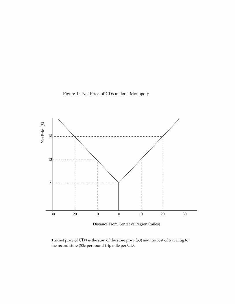
Figure 1 shows the net price of CDs for consumers living in different parts of the region.

If Bob charges $8 per CD, the net price rises from $8 for a household living next to the

music store, to $13 for a household living 10 miles from the music store, to $23 for a

household 30 miles from the store.

Figure 2 shows how the monopolist chooses the profit-maximizing output. The

monopolist’s demand curve is negatively sloped; as the store price increases, people buy

fewer CDs. The negatively sloped demand curve generates a negatively sloped marginal-

revenue curve. Profit is maximized where marginal revenue equals marginal cost, so the

monopolist produces qm units of output. If the monopolist sells qm CDs, the market-

clearing price is Pm (the point on the demand curve above qm). Total profit (revenue

less cost) is indicated by the shaded area.

Entry and Competition

Since Bob the monopolist is making positive economic profit, other entrepreneurs

will set up new music stores. Some consumers (those who live near the new music stores)

will patronize them, so Bob’s demand curve shifts to the left: at every price, he will have

fewer customers. As his demand curve and marginal-revenue curve shift to the left, his

sales volume decreases and his profits fall. In other words, entry causes competition,

which decreases sales volume and profit per firm.

0102030 10 20 30

Distance From Center of Region (miles)

8

Net

Pric

e($

)

The net price of is the sum of the store price ($8) and the cost of traveling tothe record store (50¢ per round-trip mile per

13

18

Figure 1: Net Price of CDs under a Monopoly

AverageProduction Cost

Demand = AverageRevenue

Marginal Revenue

Marginal Cost

$

Quantity of Records Per Store

qm

Pm

The profit-maximizing output (qm) is the quantity at which marginal revenue equalsmarginal cost. The monopoly price is Pm, generating profit equal to the shaded area.

Price and Quantity with Single Music StoreFigure 2:

How long will entry and the associated decreases in profit continue? Equilibrium

occurs when two conditions are satisfied. First, every firm is maximizing its profit,

producing the output at which marginal revenue equals marginal cost. Second, economic

profit is zero: The store price equals the average total cost of production.

Figure 3 shows the equilibrium situation. At an output we, marginal revenue

equals marginal cost (firms are maximizing profit), and the store price Pe equals the

average production cost (profits are zero). At the equilibrium output, the marginal

revenue curve intersects the marginal-cost curve, and the demand curve is tangent to the

average production-cost curve.

This is the theory of monopolistic competition (covered in most intermediate

microeconomics textbooks). Each music store is a monopolist within its own territory,

but its monopoly power is limited by entry and competition. Each store faces a negatively

sloped demand curve, and entry shifts the demand curve to the point at which profits are

zero. Like a perfectly competitive firm, a firm with a local monopoly earns zero

economic profit.

Efficiency Trade-Offs

There are some efficiency trade-offs associated with entry and competition. On

the one hand, entry decreases output per firm, so individual firms move upward along

their average cost curves. Scale economies are lost because output is divided among a

larger number of firms, each of which produces at a higher average cost. On the other

hand, the increase in the number of stores decreases travel distances for consumers,

decreasing travel costs.

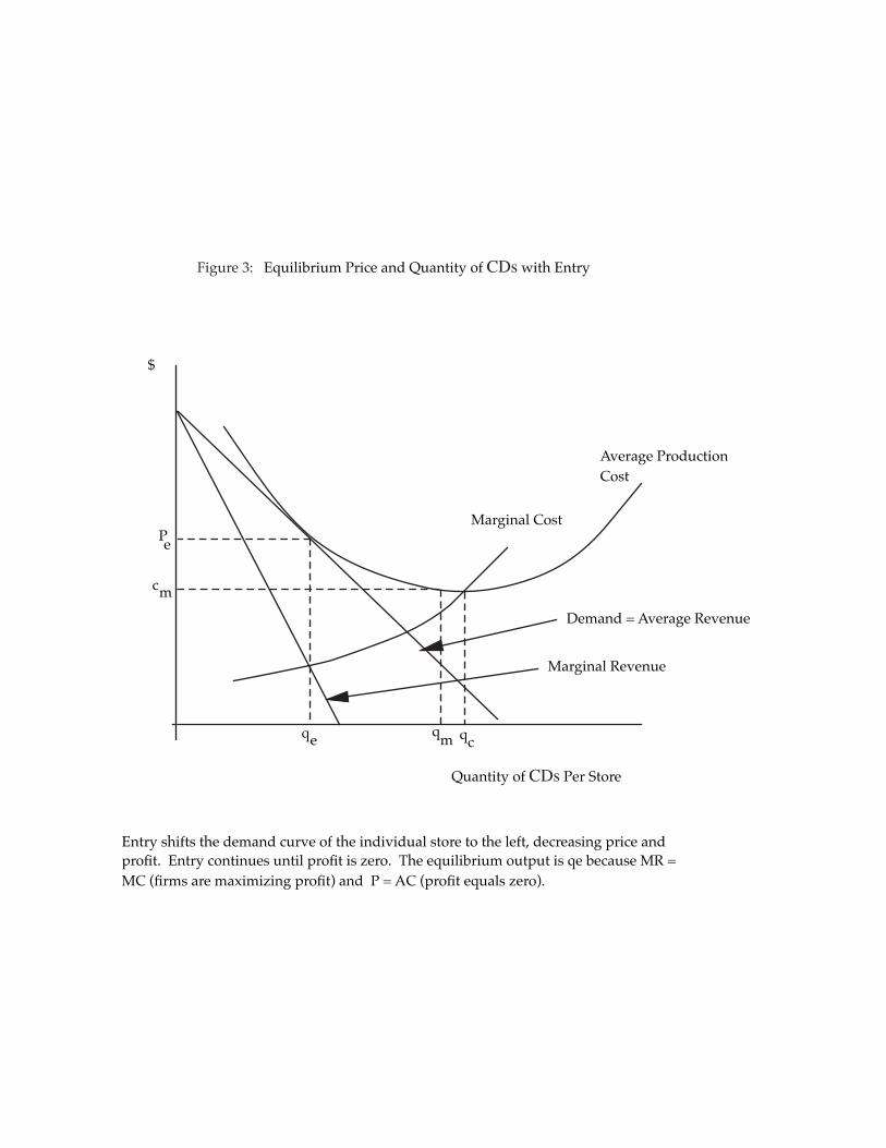
Average ProductionCost

Demand = Average Revenue

Marginal Revenue

Marginal Cost

$

Quantity of Per Store

qmqe

Pe

qc

cm

Entry shifts the demand curve of the individual store to the left, decreasing price andprofit. Entry continues until profit is zero. The equilibrium output is qe because MR =MC (firms are maximizing profit) and P = AC (profit equals zero).

Equilibrium Price and Quantity of with EntryFigure 3:

Figure 4 shows the trade-offs between production and travel costs. The average

total cost of CDs is defined as the sum of average production cost (from Figure 3) and

average travel cost. Average travel cost is the travel cost incurred by the typical CD

consumer. As the output of the music store increases, the market area increases and the

typical consumer travels a longer distance to buy CDs. Therefore, the average travel cost

increases with the output of the store. Average total cost (production cost plus travel cost)

reaches its minimum point at qt , far below the output that minimizes average production

cost (qc).

Entry decreases output per firm, generating bad news and good news. The bad

news is that average production cost increases as firms move up the average production-

cost curve. The good news is that average travel costs decrease as firms move down the

average travel-cost curve. Starting from qm in Figure 4, the good news dominates the bad

news until output per firm reaches qt . From that point on, further entry increases

production costs by more than it decreases travel costs, so average total cost increases. In

equilibrium, the output per firm drops to qe, meaning that the entry process goes “too far”

in the sense that average total cost is higher than the feasible minimum.

Figure 4 shows only one possible equilibrium outcome. For different sets of cost

and demand curves, the equilibrium output per firm might be greater than qt or equal to

qt. In other words, unless one knows something about the demand and cost curves, it’s

impossible to predict exactly where on the average total-cost curve the firm ends up.

However, we do know that (1) entry decreases output per firm and (2) in equilibrium, the

Average ProductionCost

$

Quantity of Per Store

q mqe qt

Average TotalCost

Average TravelCost

CeCt

Entry increases the number of firms and decreases output per firm. As output falls, averageproduction cost increases and average travel cost decreases. In this case, entry goes “too far”in the sense that average total cost is higher than the feasible minimum (Ct).

q c

Tradeoffs with Entry: Production Cost versus Travel CostsFigure 4

firm does not produce at the minimum point of its average production-cost curve, but at

some point to the left of the minimum point.

DETERMINANTS OF MARKET AREAS

Figure 5 shows the market areas for music stores under the assumption that there

are three stores in equilibrium. Tammy and Dick set up music stores 20 miles from Bob

and charge the same price for CDs ($6). Compared to Bob, Tammy has a lower net price

in the western third of the region, and Dick has a lower net price in the eastern third of

the region. The three music stores split the region into three equal market areas, so every

store has a circular market area with a 10-mile radius.

The market arrangement in Figure 5 has two implications for CD consumers.

First, if the spaces between the circular market areas are ignored, the maximum net price

is $11, the sum of the price charged by music stores ($6) and the maximum travel cost

($5). Second, every household patronizes the music store closest to its home. All stores

charge the same price for the same product, so a household will buy from the store with

the lowest travel costs.

An Algebraic Model of Market Areas

What factors determine the market areas of market-oriented firms? We can derive

an expression for the size of the market area with some simple algebra. The following

symbols represent the market for CDs in a region:

d = Per capita demand (number of CDs)

e = Population density (people per square mile)

Dick’s TerritoryBob’s TerritoryTammy’s Territory

0102030 10 20 30

11

Bob’s Net Price

Dick’s Net PriceTammy’s Net Price

Distance From Center of Region

6

Each store’s market area is the area over which its net price is less than the net prices ofother stores. Each store has a circular territory with a 10-mile radius.

$

Equilibrium Market AreasFigure 5

q = Output of the typical music store (CDs sold per month)

The market area of the firm (in square miles) is the territory required for the firm to sell

its target quantity (q). In other words, the market area is

M = q / ( d • e )

The denominator is the demand for CDs per square mile (also known as demand density),

equal to the quantity demanded per person (d) times the number of people per square

mile (e). In Table 2, the demand density is 200 CDs, equal to 4 CDs per person times 50

people per square mile. The market area equals the target output (q) divided by the

demand density. For example, if q = 1,000 CDs, the firm needs 5 square miles (each of

which has a demand of 200 CDs) to sell its target output.

TABLE 2 Numerical Example of Number of Stores and Market Area

Variable Symbol Numerical Example

Per capita demand (number of CDs) d 4

Population density (people per square mile) e 50

Demand density (CDs per square mile) d • e 200

Output per store (CDs sold per month) q 1,000

Market area (square miles) M = q/(d • e) 5.0

Changes in Demand and Population Density

How does an increase in the demand for CDs affect the market area of the typical

firm? An increase in per capita demand increases the volume of CDs sold per square

mile, so each firm needs a smaller market area to exploit its scale economies. For

example, if per capita demand doubles to 8 CDs per person, the market area shrinks from

5 miles (1,000/200) to 2.5 miles (1,000/400).

How does an increase in population density affect the market area? Like an

increase in per capita demand, an increase in density increases the volume of CDs sold

per square mile, so each firm needs a smaller territory to exhaust its scale economies. For

example, if population density increases to 125 people per square mile, the market area

shrinks from 5 miles (1,000/200) to 2 miles (1,000/500).

Market Area and Scale Economies

How does an increase in scale economies affect the market area? An increase in

scale economies means that average production costs continue to fall over a larger range

of output, and this causes the typical firm to produce more output. There are greater scale

economies to exploit, so the firm produces more output.

Assume for the moment that the demand for CDs is perfectly inelastic with

respect to price. In other words, consumers don’t obey the law of demand. Because an

increase in scale economies increases the output of the typical firm, it increases the

market area. Each firm needs a larger territory to exploit its now greater scale economies.

Using the numbers in Table 2, if output per store increases from 1,000 to 1,200 and the

demand density doesn’t change, the market area will increase from 5 square miles

(1,000/200) to 6 square miles (1,200/200). This is the output effect of an increase in scale

economies.

If consumers obey the law of demand, an increase in scale economies will have an

ambiguous effect on the size of the market area. The increase in scale economies will

decrease production costs and the store price, pulling down the net price of CDs to

consumers. As a result, the per capita demand for CDs will increase, and this will tend to

provide downward pressure on the firm’s market area; the firm needs a smaller territory

to sell a given output. This price effect at least partly offsets the increase in market area

caused by the increase in output per firm, so we cannot predict whether the market area

will increase or decrease. If the demand for the good is relatively inelastic, an increase in

scale economies will increase the market area.

Market Area and Travel Costs

How does a decrease in travel costs affect the output per store? Suppose the

development of a faster, cheaper travel mode decreases the monetary and time costs of

travel. Recall that travel costs prevent a firm from moving all the way down its average

production cost curve to the minimum point of the curve. The higher the travel cost, the

further a firm is from the minimum point, that is, the smaller the quantity produced. A

decrease in travel costs will reduce the strength of the force pulling the firm away from

the minimum point, so the firm will move further down the curve and produce more

output.

Assume for the moment that demand is perfectly inelastic. A decrease in travel

costs increases the quantity of product produced per firm and increases the market area

because each firm needs a larger territory to sell its now larger quantity. Using the

numbers in Table 2, if output per store increases from 1,000 to 1,400, the market area will

increase from 5 square miles (1,000/200) to 7 square miles (1,400/200). This is the output

effect of a decrease in travel costs.

If consumers obey the law of demand, a decrease in travel costs has an ambiguous

effect on the size of the market area. A decrease in travel costs decreases the net price of

CDs, increasing demand per capita (d). The increase in demand tends to reduce the firm’s

market area because the firm needs a smaller territory to sell a given quantity of output.

The price effect at least partly offsets the increase in market area caused by the increase

in output per firm, so we cannot predict whether the market area will increase or

decrease.

Parcel Post and General Stores

For an example of the effects of changes in travel costs on market areas, consider the

effects of parcel post on farm communities. Before the introduction of parcel post in

1913, farmers purchased most of their goods, including clothing and tools, in general

stores in small farm communities. The introduction of parcel post decreased the cost of

shipping goods from big-city merchants to farmers. Mail-order houses (e.g., Sears

Roebuck, Montgomery Ward) underpriced the local stores, and farmers started buying

clothing and tools from the mail-order houses. In the year following the introduction of

parcel post, the sales of Sears and Montgomery Ward quintupled, and many general

stores disappeared.

The introduction of parcel post decreased the cost of transporting clothes and

tools, increasing the market area of the typical firm. The general store with its small

market area was replaced by Sears and Wards, with their large market areas. In this case,

the output effect was stronger than the price effect, so the market area grew. Although

farmers consumed more trousers and shovels as the net prices fell, the increases in per

capita demands were not large enough to offset the output effect.

Market Area and Income

How do differences in income affect the size of market areas? Consider a region

with the following characteristics:

1. There are two cities, a poor one and a wealthy one.

2. A CD is a “normal” good (positive income elasticity of demand).

3. Land is a normal good (positive income elasticity).

Recalling the expression for market areas (M = q/(d • e)), we expect a common output per

firm in the two cities (q is the same), so the city with the larger demand per square mile

(d • e) will have the smaller market area for music stores. This is sensible because a

larger demand per square mile means a firm needs a smaller territory to exploit its scale

economies.

Which city will have a larger demand per square mile? Since a CD is a normal

good, the wealthy city will have a higher per capita demand for CDs. Since land is a

normal good, population density will be lower in the wealthy city. For example, the

wealthy may live in single-family homes and the poor may live in apartment buildings.

Because the wealthy city has a higher per capita demand and lower population density,

we can’t predict whether it will have larger or smaller market areas for music stores. The

relationship between income and market area is ambiguous because income affects per

capita demand and population density in opposite directions.

Under what circumstances will the wealthy community have a larger market area?

Suppose that the income elasticity of demand for land is large relative to the income

elasticity of demand for CDs. If so, the density effect (increased income decreases

population density) will dominate the demand effect (increased income increases per

capita demand), and the wealthy city will have a lower demand density and a larger

market area. Music stores will need a larger market area because although each

household consumes more CDs, there are many fewer households per square mile.

Table 3 shows a simple example of how differences in income affect market

areas. The income elasticity of demand for CDs is 0.50. In the wealthy city, where per

capita income is 20 percent higher, the per capita demand for CDs is 10 percent higher. In

the middle column, the income elasticity of demand for land is assumed to be 1.0.

Therefore, the wealthy city has a 20 percent higher demand for land and a 20 percent

lower population density (40 instead of 50). Given these assumptions, the wealthy city

has a lower demand density, so music stores need a larger market area to exploit their

scale economies (5.68 square miles instead of 5 square miles).

TABLE 3 Market Area with Different Income Elasticities of Demand for Land

Wealthy City

High Income Low Income

Poor City Elasticity Elasticity

Income elasticity for land 1.0 1.0 0.25

Per capita income $1,000 $1,200 $1,200

Per capita demand for CDs (d) 4 4.4 4.4

Population density (e) 50 40 47.5

Demand density (d á e) 200 176 209

Output per store (q) 1,000 1,000 1,000

Market area in square miles (q/ d • e) 5 5.68 4.78

This result depends, of course, on numerical assumptions. If the demand for land

were relatively income-inelastic, the difference in population density would be relatively

small. The demand effect would dominate the density effect, so the wealthy city would

have a smaller market area. In the third column of Table 3, the income elasticity of

demand for land is assumed to be 0.25: population density in the wealthy city is 47.5 (a 5

percent difference) instead of 40; demand density is 209 instead of 176; and the market

area is 4.78 instead of 5.68. In general, if the income elasticity for land is small relative to

the income elasticity for CDs, the wealthier city will have a smaller market area.

The Demise of Small Stores

The demise of small stores illustrates the effects of changes in population density

and transportation costs on market areas. Before the late 1800s, most goods in the United

States were purchased in small stores. People bought food in small “mom and pop”

grocery stores and purchased other goods in small general stores. The traditional

merchant was involved in every transaction, playing two roles:

1. Huckster. The merchant assisted customers in their choice of goods, providing

information on alternative products and persuading reluctant customers to buy the

goods. The merchant was an effective huckster because he knew the features of

every good in his store and was a trusted source of information about the products.

2. Haggler. The merchant negotiated with each customer over the price of a good.

The merchant was an effective haggler because she knew the cost of every good in

her store, and could quickly compute her profit margin as she negotiated with the

customer. In addition, the merchant was skillful in assessing her customers’

willingness to pay for various goods.

Since huckster and haggler skills were not easily transferred to low-skilled employees,

the merchant was involved in every transaction, and the traditional store was small.

The replacement of the small general store with larger stores suggests that the

optimum store size increased. This occurred for a number of reasons, two of which are

related to transportation costs. First, in the late 1800s and early 1900s, innovations in

urban transit increased the speed and decreased the monetary costs of intracity travel.

Second, rapid urbanization during this same period increased population density,

decreasing average travel distances (from home to store). As travel costs decreased,

merchants expanded to exploit scale economies in marketing.

As merchants developed larger stores, they adopted new marketing techniques.

New advertising and display techniques made the goods “sell themselves.” Some stores,

such as Macy’s and Marshall Field’s, used newspaper advertising to inform and persuade

consumers. Woolworth’s used plate-glass windows to display goods and attract

customers. Grocery stores displayed their goods in such a way that consumers could do

their own comparison shopping. A grocery store named Piggly Wiggly developed a floor

plan that forced customers to walk through a maze from the entrance to the exit. By

following the prescribed path from the entrance to the exit, customers were exposed to

every commodity in the store, allowing them to make their own choices. These marketing

techniques freed the merchant from acting as a huckster. Another new feature was the

single-price policy, under which the merchant charged each customer the same price and

was freed from haggling.

These two new marketing techniques freed the merchant from being involved in

every transaction, allowing an increase in the size of the store. The merchant hired low-

skilled laborers to perform the simple tasks of stocking shelves, wrapping goods, and

collecting money. A single merchant could run a self-service store with dozens of low-

wage employees, and this store could underprice the small traditional store.

Market Areas of Different Industries

Market areas vary from industry to industry, reflecting differences in travel costs,

per capita demand, and scale economies. If scale economies are large relative to per

capita demand, the industry will have a small number of firms, each of which has a large

market area. In contrast, if scale economies are small relative to per capita demand, there

will be a large number of firms with small market areas.

Consider the market areas of pizza parlors and Tibetan restaurants. Suppose that

both activities are subject to the same sort of scale economies, so the optimum output for

both types of restaurants is 200 meals per day. If the total demand for pizza is 10,000

meals per day, the region will have 50 pizza parlors (10,000/200). If the total demand for

Tibetan food is 200 meals per day, a single Tibetan restaurant will serve the entire region.

The market area is not determined by scale economies per se, but by scale economies

relative to per capita demand.

CENTRAL PLACE THEORY

Central place theory, which was developed by Christaller (translated in 1966) and

refined by Losch (translated in 1954), is used to predict the number, size, and scope of

cities in a region. The theory is based on a simple extension of market-area analysis.

Market areas vary from industry to industry, depending on scale economies and per

capita demand, so every industry has a different location pattern. Central place theory

shows how the location patterns of different industries are merged to form a regional

system of cities. The theory answers two questions about cities in a regional economy:

1. How many cities will develop?

2. Why are some cities larger than others?

A Simple Central Place Model

Consider a region with three consumer products: CDs, pizzas, and jewelry. The

region has the following characteristics:

1. Population density. The initial distribution of population is uniform. The total

population of the region is 80,000.

2. No shopping externalities. As discussed in Chapter 2, shopping externalities

normally occur with complementary goods (one-stop shopping) and imperfect

substitutes (comparison shopping). The simple central place model assumes that

there are no shopping externalities.

3. Ubiquitous inputs. All inputs are available at all locations at the same prices.

4. Uniform demand. For each product, per capita demand is the same throughout the

region.

5. Number of stores. The three goods have different per capita demands and scale

economies:

a. Jewelry. Scale economies are large relative to per capita demand. Every

jewelry store requires a population of 80,000, so a single jeweler will serve the

entire region.

b. Compact discs. Scale economies are moderate relative to per capita demand.

Every music store requires a population of 20,000, so there will be four music

stores in the region.

c. Pizza. Scale economies are small relative to per capita demand. Every pizza

parlor requires a population of 5,000, so there will be 16 pizza parlors in the

region.

The central place model is a model of market-oriented firms, defined earlier in the

book as firms that base their location decisions exclusively on access to their consumers.

Because all inputs are ubiquitous, the firms ignore input costs in their location decisions.

The single jeweler will locate at the center of the region. Because production costs are the

same at all locations (all inputs are ubiquitous), the jeweler will minimize its total costs

by minimizing its travel costs. According to the principle of median location (discussed

earlier in the book), travel costs are minimized at the median location. Because

population density is uniform, the median location is the center of the region and the

jeweler will locate there. A city will develop around the jewelry store. Jewelry workers

will locate near the store to economize on commuting costs. The population density near

the jeweler will increase, generating a city (a place of relatively high density) at the

center of the region. In Figure 6, a city develops at point L.

The music stores will carve up the region into market areas, causing the

development of additional cities. If the region’s population density were uniform, music

firms would carve out four equal market areas. However, because there is a city

surrounding the jeweler in the center of the region, there will be enough demand to

support more than one music store in city L. If city L along with the surrounding area has

enough people to support two music stores, the two other music stores will split the rest

of the region into two market areas. In Figure 6, two more cities develop at the locations

marked with an M.

The pizza parlors will also carve up the region into market areas, causing the

development of more cities. Because the population density is higher in the cities that

develop around the jewelry store and the music stores, there will be more than one pizza

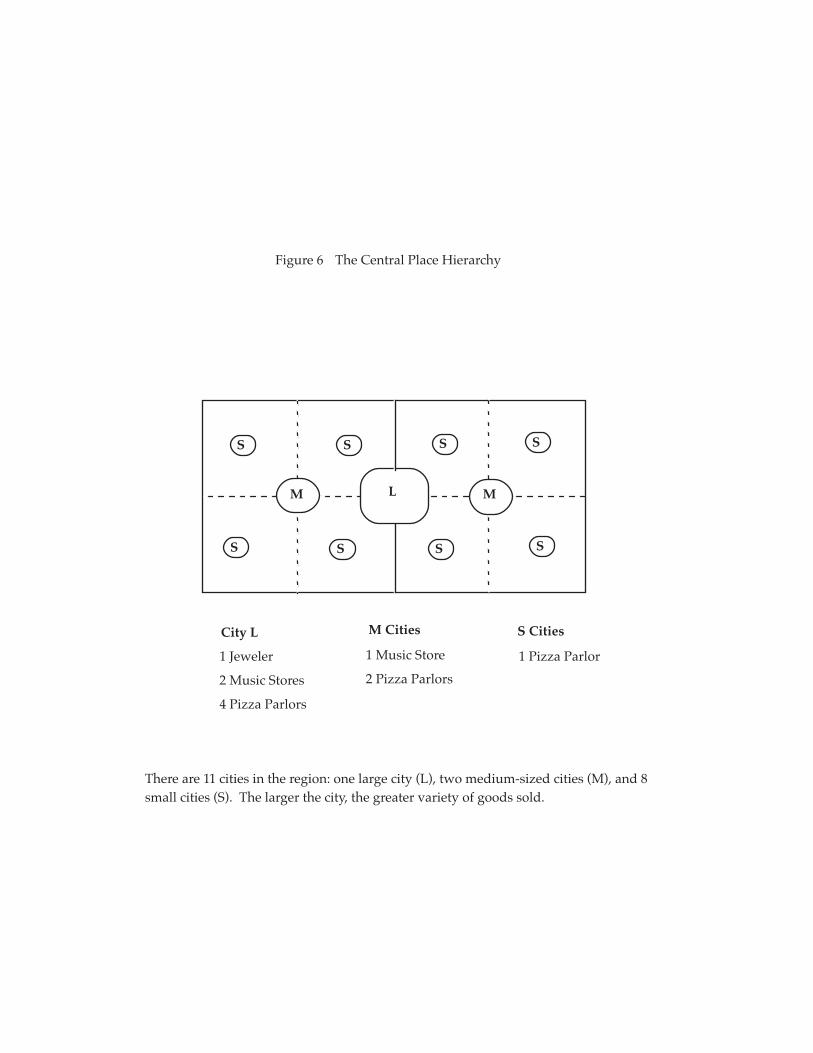
Figure 6

parlor in L and the two M cities. Suppose that L will support four pizza parlors, and each

of the M cities will support two pizza parlors. If so, a total of eight pizza parlors will

locate in cities L and M. The remaining eight pizza parlors will divide the rest of the

region into eight market areas, causing the development of eight additional cities (the

places marked with an S in Figure 6).

The rectangular region has a total of 11 cities. The large city at the center of the

region sells jewelry, CDs, and pizza. City L has a population of 20,000, meaning that it is

large enough to support four pizza parlors (5,000 people per pizza parlor). The city sells

CDs to consumers from the four surrounding S cities, so the total number of CD

consumers is 40,000 (20,000 from L and 5,000 each from four S cities), enough to

support two music stores. The two medium-sized cities sell CDs and pizza. Each of the M

cities has a population of 10,000, meaning that each city is large enough to support two

pizza parlors. Each city sells CDs to consumers from two nearby S cities, so the total

number of CD consumers in each M city is 20,000 (10,000 from M and 5,000 each from

two S cities), enough to support one music store per M city. The eight small cities sell

only pizza. Each of the S cities has a population of 5,000, meaning that each city can

support one pizza parlor.

Figure 7 shows the size distribution of cities in the region. The vertical axis

measures city size (population), and the horizontal axis measures the rank of the city. The

largest city (L) has a population of 20,000; the second and third largest cities (M cities)

have populations of 10,000; and the fourth through the eleventh largest cities have

populations of 5,000.

Figure 7

The simple central place model generates a hierarchical system of cities. There

are three distinct types of cities: L (high order),M(medium order), and S (low order). The

larger the city, the greater the variety of goods sold. Each city imports goods from higher-

order cities and exports goods to lower-order cities. Cities of the same order do not

interact. For example, an M city imports jewelry from L and exports CDs to S cities, but

does not interact with the other M city. Similarly, an S city imports jewelry from L and

CDs from either L or an M city, but does not trade with other S cities. The system of

cities is hierarchical in the sense that there are distinct types of cities and distinct patterns

of trade dominance.

The simple central place model provides some important insights into how the

market-area decisions of firms combine to generate the urban hierarchy. Here are some

lessons from central place theory.

1. Diversity and scale economies. The region’s cities differ in size and scope. This

diversity occurs because the three consumer products have different scale economies

relative to per capita demand, so they have different market areas. To explain the

importance of differences in relative scale economies, suppose that the three goods

have the same scale economies relative to per capita demand, so the region has 16

jewelers, 16 music stores, and 16 pizza parlors. The market areas of the three goods

would coincide, so the region would have 16 identical cities, each of which would

provide all three goods. In other words, if there are no differences in scale economies

relative to per capita demand, the region’s cities will be identical.

2. Large means few. The region has a small number of large cities and a large number

of small cities. Why isn’t there a large number of large cities and a small number of

small cities? A city is relatively large if it provides more goods than a smaller city.

The extra goods provided by a large city are those goods that are subject to relatively

large scale economies. Since there are few stores selling the goods subject to

relatively large scale economies, few cities can be large. In the simple central place

model, the L city is larger than an M city because L sells CDs, pizza, and jewelry.

Since there is only one jewelry store in the region, there is only one city larger than

the M cities.

3. Shopping paths. Consumers travel to bigger cities, not to smaller cities or cities of

the same size. For example, consumers from an M city travel to L to buy jewelry,

but do not travel to the other M city or an S city to consume CDs or pizza. Instead,

they buy CDs and pizza in their own city. Similarly, consumers in S cities travel to

larger cities for jewelry and CDs, but do not shop in other S cities.

Relaxing the Assumptions

Several of the assumptions of the simple central place model are unrealistic. This

section relaxes some of the assumptions, addressing two questions. First, does a more

realistic model generate the same hierarchical pattern of cities? Second, does a more

realistic model have more or fewer cities? The simple model assumes that the CDs from

different music stores are perfect substitutes. There is no need for comparison shopping,

and thus no tendency for music stores to cluster. Suppose that CDs and music stores are

replaced by clothing and clothing stores. People shopping for clothes like to compare the

clothes from different firms, and this will encourage the clothing stores to cluster rather

than disperse like the music stores. If the optimum cluster is four clothing stores, the

stores will cluster at the center of the region. The region will have only two types of

cities, large ones (with jewelers, clothing stores, and pizza parlors) and small ones (with

pizza parlors). The presence of imperfect substitutes reduces the equilibrium number of

cities from 11 to 9 because clothing stores compromise on their “ideal” (central place)

locations to exploit the shopping externalities. Although comparison shopping decreases

the number of cities, it does not disrupt the hierarchical pattern of cities.

Another assumption of the simple model is that the three products are not

complementary goods. Suppose instead that pizza and CDs are complementary, so that

the typical consumer purchases a CD and a pizza on the same shopping trip. If so, music

stores and pizza parlors will pair up to facilitate one-stop shopping. If pizza parlors

cannot survive without a companion music store, there will be only two types of cities in

the region: large (with jewelry, CDs, and pizza) and medium (with CDs and pizza). Pizza

parlors compromise on their ideal (central place) locations to exploit the shopping

externalities associated with one-stop shopping, so the equilibrium number of cities

decreases from 11 to 3. The presence of complementary goods does not, however, disrupt

the urban hierarchy.

One of the assumptions of the simple central place model is that per capita

demand does not vary with city size. Systematic variation in per capita demand may

disrupt the urban hierarchy. Suppose we replace pizzas with grits, a good for which per

capita demand is high in smaller cities and zero in large cities. Since there will be no grits

restaurants in the large city, the urban hierarchy will be disrupted: the medium-size and

the small cities supply goods that are not available in the large city. Of course, if per

capita demands increase with city size (for example, theater or opera), goods will be more

concentrated in larger cities and this sort of variation in demand will not disrupt the

hierarchy, but will increase the variety of goods more rapidly as we move up the

hierarchy.

Other Types of Industry

Central place theory is applicable to market-oriented firms. The objective of a

market-oriented firm is to minimize the travel costs of its consumers. The market-

oriented firm is not concerned about (1) the cost of transporting its inputs or (2) the costs

of local inputs. Central place theory predicts the pattern of cities that would result if all

firms were market-oriented.

As explained in Chapter 2 of Urban Economics (Sixth Edition), there are two

other types of firms, resource-oriented firms and input-oriented firms. For the resource-

oriented firm (e.g., the producer of baseball bats), the cost of transporting raw materials is

relatively high, so the firm locates near its input sources. For the input-oriented firm, the

costs of local inputs vary across space, and the firm locates near sources of inexpensive

labor, energy, or intermediate goods.

The location decisions of resource-oriented firms may disrupt the central place

hierarchy. Suppose that a bat factory is located near the coastal forests of the region.

Once the coastal city is established it may attract some market-oriented firms (e.g., pizza

parlors). In addition to the three types of cities described above (large, medium, and

small) there will be a coastal city, with a bat factory and pizza parlors. The urban

hierarchy is disrupted because the coastal city has one activity (bat production) not

available in the largest city.

It is possible that the bat factory will not disrupt the region’s urban hierarchy.

Suppose that the coastal city becomes large enough that it becomes the median location

for the jeweler. If so, the coastal city will have all four types of activities (jewelry, bats,

CDs, and pizza). The medium-size cities will have two activities (pizza and CDs), and the

small cities will have only one activity (pizzas). In this case, the hierarchy is preserved

because the coastal city takes the place of city L.

The same arguments apply to input-oriented activities such as textile firms (labor-

oriented), aluminum producers (energy-oriented), corporate headquarters (oriented to

intermediate inputs), and firms engaging in research and development (oriented to

amenities valued by engineers and scientists). If the input-oriented firm locates near its

input source, the resulting city will have some goods that are not available in the largest

city. If, however, the resulting city becomes the median location in the region, it may

replace city L as the largest city in the region.

CENTRAL PLACE THEORY AND THE REALWORLD

While central place theory is not literally true for many regions, it provides a

useful way of thinking about a regional system of cities. The theory identifies the market

forces that generate a hierarchical system of cities. It explains why some cities are larger

than others, and why the set of goods sold in a particular city is typically a subset of the

goods sold in a larger city. Exceptions to the hierarchical pattern result from (1)

systematic variation in per capita demand and (2) the location decisions of firms oriented

toward raw materials and local inputs.

Empirical Studies of Central Place Systems

Table 4 shows the results of an empirical study of central place theory. Berry and

Garrison (1958) examined the economic activities of urban places in Snohomish County,

Washington. They concluded that the dozens of communities in the area could be divided

into three distinct types of urban places: towns (high order), villages (medium order), and

hamlets (low order). The largest urban place, a town, was about twice as large as a

village, which was in turn about twice as large as a hamlet. There were about half as

many towns as villages, and about half as many villages as hamlets. As one moves down

the hierarchy, the number of establishments and the number of functions decrease, which

is exactly what is predicted by central place theory. Berry and Garrison concluded that

the system of urban places was indeed hierarchical, with individual communities

exporting to lower-order places and importing from higher-order places.

TABLE 4 The Urban Hierarchy in Snohomish County, Washington

Type of Place

Town Village Hamlet

Number of places 4 9 20

Average population 2,433 948 417

Average number of establishments per place 149 54.4 6.9

Average number of functions per place 59.8 32.1 5.9

Average number of establishments per function 2.5 1.7 1.2

Source: Brian J. L. Berry and William Garrison, “The Functional Bases of the Central

Place Hierarchy,” Economic Geography 34, pp. 145-54, 1958, Clark University.

Most of the empirical studies of central place theory examine systems of small

towns in agricultural regions. Such regions have little industrial activity, so most firms

are oriented toward the local market, not toward natural resources or local inputs. What

about the national economy? As explained earlier, the central place hierarchy is disrupted

by the location choices of resource-oriented firms and input-oriented firms. Since a large

fraction of national employment comes from resource-oriented and input-oriented

activities, it would be quite surprising if a study of the national economy provided much

support for the simple central place model.

SUMMARY

1. Market-oriented firms are involved in monopolistic competition or spatial

competition. Each has a local monopoly, but its monopoly power is limited by entry

and competition from other firms. In equilibrium, every firm produces the quantity

such that marginal revenue equals marginal cost and each firm makes zero economic

profit.

2. The market area of an industry depends on the quantity produced per firm, per capita

demand, and population density.

3. Central place theory, which is based on market-area analysis, predicts that the

regional system of cities will be hierarchical, with a small number of large cities and a

large number of small cities. The set of goods sold in smaller cities will be a subset of

the goods sold in larger cities.

4. If the assumptions of the simple central place theory are relaxed to allow imperfect

substitutes (comparison shopping) and complements (one-stop shopping), the

equilibrium number of cities may decrease, but the urban hierarchy will not be

disrupted.

5. Central place theory is not applicable to resource-oriented firms and firms oriented

toward local inputs. The introduction of such firms into the central place model may

disrupt the urban hierarchy.

EXERCISES AND DISCUSSION QUESTIONS

1. The discussion of the market area of music stores assumed that store owners Bob,

Tammy, and Dick had the same production costs. As a result, households patronized the

store nearest their homes. Suppose that Bob discovers a new way of marketing CDs that

cuts his production cost (and store price) in half, from $6 to $3. Tammy and Dick

continue to sell CDs for $6.

a. How does the decrease in production cost affect Bob’s market area?

b. What is the net price at the border between Bob’s and Tammy’s market area?

c. Will each household still patronize the firm closest to its residence?

2. Consider the market area of food stores in a region described by the following

assumptions: (i ) The per capita demand for food is 30 units; (ii) Population density is

40 people per square mile; (iii) The land area of the region is 100 square miles; (iv) The

output of the typical food store is 6,000 units.

a. How many food stores will there be in the region?

b. How large is the market area of the typical food store?

3. Consider the market areas of hardware stores in two independent regions, Low and

High. The average production-cost (APC) curves of the two regions reach their minimum

points at the same level of output (1,000 units), but because Low has lower input costs,

the minimum point of its APC curve has a lower average cost (its average cost of 1,000

units is $1 instead of $2).Will the market area in Low be larger, smaller, or the same as

the market area in High? If you don’t have enough information to answer the question,

indicate what additional information you need and how you would use it.

4. Consider a regional economy with two cities. The two cities have the same population,

but the average household income in city H exceeds that in city L. The residents of H and

L consume Y. The characteristics of Y are as follows: The average production-cost

(APC) curve is U-shaped; The APC curve is the same at all locations; Y is a standardized

product, with no close substitutes or complements; all households have the same tastes

for Y; Y is inferior (negative income elasticity).

a. How will the size of the average market area of Y in city H compare to the size

of the average market area in city L?

b. How would your response to (a) differ if the APC curve were a horizontal line?

5. Suppose that you intend to purchase the franchise rights for a pizza parlor. The

franchiser has divided your region into two areas of equal size: H is a high-income area,

and L is a low-income area Suppose that the income elasticity of demand for pizza is

zero: the consumption of pizza is independent of income. The income elasticity of

demand for land is 1.0. Your objective is to maximize the quantity of pizzas sold.

a. Which of the two franchises will you choose?

b. How would your response to (a) change if the income elasticity of demand for

pizza is 1.5?

6. In the example based on the data in Table 3, the implicit assumption is that travel costs

were the same in the two cities. Suppose that the opportunity cost of travel is higher in

the wealthy city. How might this change the market areas in the wealthy city?

7. Consider the city of Vaudeville, where initially all video consumers travel to video

outlets to rent videos. Suppose that when the video outlets offer home delivery, all video

consumers switch to home delivery.

a. Under what circumstances is the switch to home delivery rational?

b. In what type of cities would you expect home delivery to be efficient?

8. In 1930, most rural children walked to school. By 1980, most of them rode school

buses. Would you expect the average “market area” of rural schools to increase or

decrease as a result of the school bus?

9. The introduction of parcel post decreased transportation costs and increased the market

area of the typical firm. Can you think of any good for which a decrease in transportation

costs is likely to decrease the market area?

10. In the city of Metro, retail firms locate either in the central area of the city or in one of

the suburban subcenters. There are two retail goods sold in the city, A and B. The per

capita demands for the two goods are equal. The scale economies associated with the

production and sale of A are large relative to the scale economies associated with B.

Where in the city will the firms selling A and B locate?

11. Consider a city with a uniform distribution of population where every household

consumes the same number of video rentals. The city is two miles long and two miles

wide. The mayor recently stated her policy for the location of video rental outlets: “A

video outlet reaches the minimum point of its average production-cost curve at an output

of 1,000 units. Since the total demand for video rentals is 4,000 units, we should have

four video outlets. Since the distribution of population is uniform, the video outlets

should be distributed uniformly throughout the city, with every outlet at the center of a

one-square-mile market area.” Comment on the mayor’s policy. Will it lead to an

efficient distribution of video outlets?

12. In the city of Zone, the actual number of grocery stores is less than the number that

would occur in the absence of zoning. A recent survey of grocery prices suggests that

Zone consumers pay less for groceries than people in a similar city without zoning. For

example, the prices of Spam and Velveeta are 5 percent lower in Zone.

a. Is there any reason to doubt the validity of the survey?

b. Suppose that the survey is valid. Does the zoning policy make the residents of

Zone better or worse off?

13. A developer has requested a permit to build a drugstore in a rapidly growing part of

your city. Your mission is to figure out whether the new drugstore is appropriate. What

information do you need, and how would you use it?

14. Explain why poor areas of cities typically are served by small grocery stores, not by

large grocery-store chains.

15. Consider a region in which all firms are market-oriented (all employment is in retail

outlets). There are no shopping externalities, and all retail activities are subject to the

same degree of internal scale economies. In the last 10 years, the region’s rank-size curve

(with city rank on the horizontal axis and city size on the vertical axis) has become

flatter.

a. What changes in market areas are lurking behind the flattening of the rank-size

curve?

b. Provide an explanation for the changes in the market areas lurking behind the

flattening of the rank-size curve.

16. Mr. Wizard, a regional planner, recently made the following statement: “If my

assumptions are correct, all cities in this region will eventually be identical. They will be

the same size and will sell the same set of goods.”

a. Assuming that Mr. Wizard’s reasoning is correct, what are his assumptions?

b. Are Mr. Wizard’s assumptions realistic?

17. Some people claim that state capitals (e.g., Sacramento, California; Salem, Oregon;

Olympia, Washington) are boring cities. Specifically, it is claimed that these cities have

fewer goods than one finds in other cities of equal size. After checking a map to see

where each of these capital cities is located, use central place theory to explain why they

might be considered boring.

REFERENCES

1. Berry, Brian J. L., and William L. Garrison. “The Functional Bases of the Central

Place Hierarchy.” Economic Geography 34 (1958), pp. 145_54. An empirical analysis

of central place theory.

2. Christaller, Walter. Central Places in Southern Germany, trans. C.W. Baskin.

Englewood, NJ: Prentice Hall, 1966.

3. Losch, August. The Economics of Location. New Haven, CT: Yale University Press,

1954.