Mark E. Harmon Richardson Chair & Professor Forest ... E. Harmon Richardson Chair & Professor Forest...
32
Mark E. Harmon Richardson Chair & Professor Forest Ecosystems and Society Oregon State University Corvallis, OR
Transcript of Mark E. Harmon Richardson Chair & Professor Forest ... E. Harmon Richardson Chair & Professor Forest...

Mark E. Harmon Richardson Chair & Professor
Forest Ecosystems and Society Oregon State University
Corvallis, OR

Main points The basic ecosystem science behind carbon dynamics
in forests is relatively straightforward (really!)
This science doesn’t seem to be applied routinely in the policy arena
This mismatch is undermining the potential of the forest sector in helping to mitigate greenhouse gases in the atmosphere

Basic Principles
Presenter
Presentation Notes
There are just a few basic principles that can be used to understand how carbon works in the forest sector.

Conservation of mass law
Carbon
Ocean Ocean
Land surface Land surface
Rocks Rocks
Atmosphere Atmosphere
Presenter
Presentation Notes
The starting point is the conservation of mass law. We have only so much carbon on Earth and new carbon can’t be created or destroyed. There are four major pools that it can be stored and increasing in one means it must be decreased somewhere else. In this case increasing carbon stored in the land surface means less in the atmosphere. Conversely less in the land surface means more in the atmosphere, at least until it goes somewhere else. So the key thing to understand it how something influences the carbon store. There are many processes controlling these, but ultimately what one needs to know about is stores and how they change.

Which forest stores more carbon? OG=600 MgC/ha
Harvested forest=325 MgC/ha Young forest=260 MgC/ha Forest products= 65 MgC/ha
At current uptake rates 130 years to reach OG store
Presenter
Presentation Notes
Applying conservation of mass shows us that converting an old-growth forest with high stores to a young forest with forest products must add carbon to the atmosphere. The higher rate of net carbon uptake of the younger forest is irrelevant because it would have to be vastly larger that it is (over 100 times higher) for the stores to be the same (which of course they are not).

Live Plants
Soil
Wood Products
Outside forest system
Photosynthesis
photosynthesis
Timber harvest mortality
Soil formation
Respiration and combustion
Dead Plants
Presenter
Presentation Notes
What controls the amount of carbon stored in a forest? The forest carbon system can be envisioned as a series of leaky buckets. The amount stored in each bucket depends on the amount coming in versus the proportion leaking out. Carbon enters the forest systems via photosynthesis. Carbon leaks out via many processes, but the main ones are respiration and combustion. Note that the input-output relationship is the same for all the carbon pools in a forest and for the forest sector as a whole.

Presenter
Presentation Notes
Let’s look at a leaky bucket and see how it works. Note that the inputs and outputs are going on at the same time. If it starts with nothing in the bucket it will begin to fill, but it will not overtop as in time amount coming in is the same as going out.

5 Medium
leaks
5 Large leaks
2 Large leaks
7 Small leaks
Presenter
Presentation Notes
In a leaky bucket the number and size of the leaks determines the amount stored if the input is constant. Here the input amount was constant for all the buckets.
0 0.5
1 1.5
2 2.5
3 3.5
4 4.5
0 0.1 0.2 0.3 0.4 0.5
Stor
e (L
)
Leakiness k (per sec)
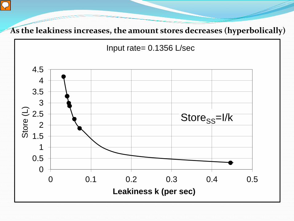
Input rate= 0.1356 L/sec
StoreSS=I/k
As the leakiness increases, the amount stores decreases (hyperbolically)
Presenter
Presentation Notes
Here is a plot of the results from the leaky buckets. As the leakiness increases, the amount that can be stored decreases.

0
0.5
1
1.5
2
2.5
3
3.5
0.075 0.095 0.115 0.135 0.155
Stor
e (L
)
Input rate (L/sec)
StoreSS= I/k
As the input increases, the amount stored increases (linearly)
Presenter
Presentation Notes
The amount stored is also a function of the size of the input. In a leaky bucket the input does not have the ideal linear effect on stores, in part because the leakiness is not a function of the volume, but of the area of the bottom, hence a larger store is less leaky for a given hole size than a smaller store.

The fewer and smaller the holes the more stored
0
100
200
300
400
500
600
0 100 200 300 400 500
Css
(Mg/
ha)
Time between disturbances
severity = 0 severity= 0.05
severity=0.1 severity=0.2
severity=0.5
Full input (NPP) returns in 25 years
Presenter
Presentation Notes
Here we take the leaky bucket and turn it into a mathematical model. As the time between disturbances increases the number of leaks decreases. As the severity of disturbances increases the hole size increases. Even when a disturbance does not directly remove carbon (severity equals zero), it has an effect. By setting NPP back, even if it takes as little as 25 years to recover as in this example, a disturbance can reduce the amount of carbon in a landscape.

Can a steady-state have a carbon debt or credit?
Debit
Credit
0
100
200
300
400
500
600
700
2100 2200 2300 2400 2500
Ecos
yste
m C
sto
re (M
gC/h
a)
Year
Stand level
Presenter
Presentation Notes
We start with one stand and can see that it is quite variable, with a large amplitude of change, going down when the stand is harvested (in this case every 100 years) and going up as it regrows. This has been used in the debate about biofuels and whether a carbon debt or carbon credit is created.

Can a steady-state have a carbon debt or credit? Not really, as it makes no sense
Debit
Credit
Presenter
Presentation Notes
But in this system carbon is stable at the landscape level? That is because we are averaging stands of different ages. The point is that decreases in some stands are offset by increases others. This offsetting effect is at the maximum when there is a regulated disturbance system, that is disturbances at regular intervals. But synchrony of stands is also important. In the preceding slide we assumed that stands were perfectly offsetting each other. In this system the idea of a carbon debt or credit makes absolutely no sense.

0
100
200
300
400
500
600
1900 2000 2100 2200 2300 2400 2500
Ecos
yste
m c
arbo
n st
ore
(Mg/
ha)
Year
60 yr continued
60 y to 30 y
60 y to 120 y
Going from one steady-state to another can create either a carbon debt or credit!
This is the real issue we need to evaluate
Presenter
Presentation Notes
What we really need to think about is how a change impacts the long-term average store of carbon over a large area. In this situation one can have a carbon debit or a credit or can have no change. It really depends on the relative changes in input or leakiness.

Thinning adds more carbon to forests than not thinning

Forest Thinning Increases the health and growth of
trees Faster growing trees means more
carbon can be stored Before After
1 ‹ 1.1
Presenter
Presentation Notes
The basic idea is this and below we see the mathematical relationship

Wait a minute! Aren’t there fewer trees after thinning?
Before After
1 ‹ 1.1 incomplete comparison
1 x 100 ≈ 1.1 x 90 complete comparison
To store more total growth must increase, not stay the same
Presenter
Presentation Notes
But the previous slide left off some very key ideas. It not just a function of the growth rate of individuals, it is also a function of the number of individuals.

For total growth to increase the following must be true
The recovery of tree production after thinning must be instantaneous (BUT IT IS NOT)
Thinning must increase the total amount of resources available to trees so that total production of thinned trees can increase (HOW?)
Before
thinning
After thinning
New resources???
Presenter
Presentation Notes
Since the number of trees goes down after thinning, there must be something else going on if the fewer remaining trees are going to have higher total growth.
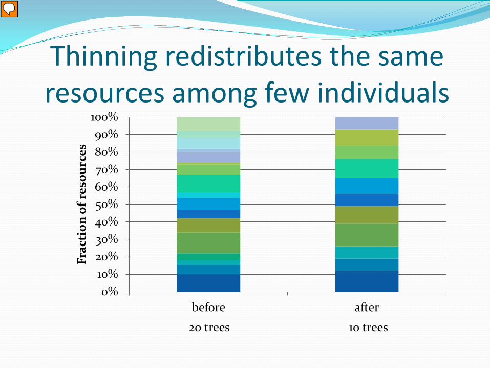
Thinning redistributes the same resources among few individuals
0% 10% 20% 30% 40% 50% 60% 70% 80% 90%
100%
before after
Frac
tion
of r
esou
rces
20 trees 10 trees
Presenter
Presentation Notes
Here is what actually happens when a forest is thinned. Fewer trees share the same amount of resources. They therefore grow faster, but since the total amount of resources have not increased the total growth can not be higher than before thinning.

0
2
4
6
8
10
12
14
16
2000 2050 2100 2150 2200 2250 2300Year
NP
P (
Mg C
/ha
50 year with thin50 year no thin
Thinned Not thinned NPP 7.93 8.83 11% less Mg C/ha/y
Thinning does not increase the input to the forest!
Presenter
Presentation Notes
Here are some results from a simulation model. Note that when the forest is thinned, in this case 25% of the live carbon is thinned 25 years after clear-cut harvesting. Note that although the input (NPP) to the forest in the thinned forest recovers eventually, it is 11% less on average than the unthinned forest.

Thinned Not thinned Store 298 341 13% less Mg C/ha
0
100
200
300
400
500
600
2000 2050 2100 2150 2200 2250 2300
Year
C s
tore
(M
g/h
50 year no thin50 year thinned
Thinning decreases forest carbon stores
Presenter
Presentation Notes
This is the effect on carbon stores of thinning, it decreases the average store because it has lower inputs (11%) and increased leakiness (2%).
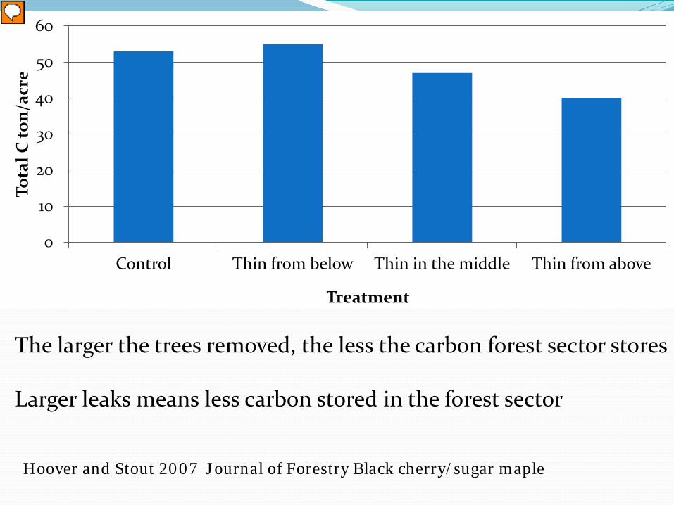
Hoover and Stout 2007 Journal of Forestry Black cherry/sugar maple
The larger the trees removed, the less the carbon forest sector stores Larger leaks means less carbon stored in the forest sector
0
10
20
30
40
50
60
Control Thin from below Thin in the middle Thin from above
Tota
l C to
n/ac
re
Treatment
Presenter
Presentation Notes
The results are not just restricted to models; here are some results from a field study.

Keyser 2010 Canadian Journal of Forest Research Yellow poplar
Presenter
Presentation Notes
If thinning increased carbon stores, then one would expect that as the amount of thinning increased (as indicated by residual basal area-RBA) that the store in live biomass would increase. But we do not see this.

Other issues needing to be addressed ASAP Failure to observe conservation of mass Exclusion of pools, processes, or key factors Irrelevant processes (hiding real relationship) Failing to give initial conditions or BAU Improper or inconsistent scaling in space & time Instantaneous uptake/release versus long-term stores Inconsistent frameworks Logical incongruities
Presenter
Presentation Notes
The list of problems in some of the “science” being used in setting forest carbon policy is extensive.
Conclusions To be credible carbon policy must be based on science
(real world) otherwise it will not deliver the desired goal
There are many objectives of forest management Some will have carbon costs If these costs are not recognized then policies to
counter or reduce these costs can not be developed

http://landcarb.forestry.oregonstate.edu/
Presenter
Presentation Notes
If you are interested in learning more about how carbon acts in the forest sector you can go to this website.


Landowner’s forest resource management practices for improving carbon accumulation are categorized as follows (US EPA, 2010): i)Forest conservation: called avoided deforestation or forest preservation, means not clearing a forest, ii)Afforestation/Reforestation, and iii)Intermediate forest management, called improved forest management or active forest management, means changing management approaches so that standing volume in the forest is increased. Practices such as forest thinning can both reduce fire risk and stimulate growth that, over time, increases carbon storage. iv)Biomass energy – Using fuel from wood and biomass in place of fossil fuel. v)Carbon storage in forest products and substitution: Storing carbon in long-lived forest products (such as lumber) and substituting forest products for products (such as steel and concrete) whose manufacture releases much more CO2 than does the processing of wood.
Forest management practices for carbon sequestration
Presenter
Presentation Notes
Let’s examine the text that has been bolded.

Forest ecosystem Forest products Fossil carbon
Atmosphere
Aquatic systems
The forest sector
Presenter
Presentation Notes
Here are the basic pools of the forest sector. While fossil carbon is outside the forest sector, it is influenced by substitutions related to the forest sector as shown by the dashed line.

The Math of Leaky Buckets
Css=I/k
I is the input rate k is the proportional loss rate
Css
I
O
Presenter
Presentation Notes
The steady-state carbon store is a function of the input as well as the rate-constant of loss. Recall that this follows for a steady-state system because inputs equal outputs and outputs are a function of the store and the proportion being lost, or as we call it here the rate-constant of loss, k.

Thinned Not thinned Store 346 530 35% less Mg C/ha
0
100
200
300
400
500
600
700
800
900
2000 2050 2100 2150 2200 2250 2300
Year
C s
tore
(M
g/h
no thinningthinned
Presenter
Presentation Notes
Similar effects when forests are thinned over longer intervals.
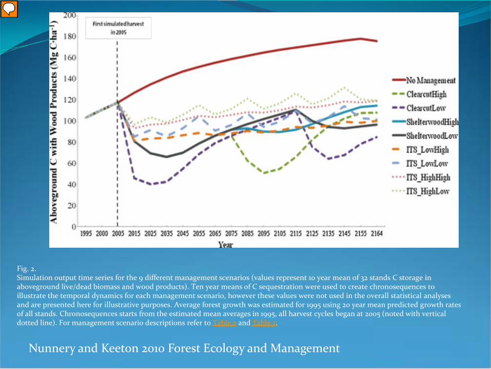
Fig. 2. Simulation output time series for the 9 different management scenarios (values represent 10 year mean of 32 stands C storage in aboveground live/dead biomass and wood products). Ten year means of C sequestration were used to create chronosequences to illustrate the temporal dynamics for each management scenario, however these values were not used in the overall statistical analyses and are presented here for illustrative purposes. Average forest growth was estimated for 1995 using 20 year mean predicted growth rates of all stands. Chronosequences starts from the estimated mean averages in 1995, all harvest cycles began at 2005 (noted with vertical dotted line). For management scenario descriptions refer to Table 2 and Table 3.
Nunnery and Keeton 2010 Forest Ecology and Management
Presenter
Presentation Notes
Others have found the exact same response.