Stress testing and financial stabilityMark D. FloodDepartment of FinanceUniversity of Maryland

Center for Latin American Monetary Studies (CEMLA)Course on Financial StabilityMexico City, 19 September 2019

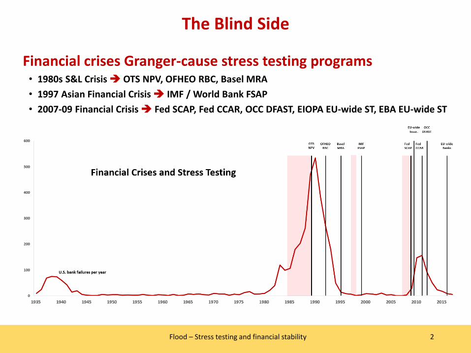
The Blind Side

2Flood – Stress testing and financial stability

Financial crises Granger-cause stress testing programs• 1980s S&L Crisis OTS NPV, OFHEO RBC, Basel MRA• 1997 Asian Financial Crisis IMF / World Bank FSAP• 2007-09 Financial Crisis Fed SCAP, Fed CCAR, OCC DFAST, EIOPA EU-wide ST, EBA EU-wide ST

Supervisory Stress Testing v1.0

3Flood – Stress testing and financial stability

Some examples• 1992 OFHEO housing scenario• 1996 Basel market risk amendment• 2001 IMF Financial Sector Assessment Programs (FSAPs)

Characteristics• Microprudential only• Focus on historical scenarios (“fighting the last war”)• Scenarios and models inconsistent across firms• Extrapolating from value-at-risk (VaR)

Supervisory Stress Testing v2.0

4Flood – Stress testing and financial stability

Some examples• 2009 Supervisory Capital Assessment Program (SCAP)• Comprehensive Capital Assessment and Review (CCAR)• Dodd-Frank Act Stress Tests (DFAST)• European Banking Authority (EBA) stress tests

Characteristics• Detailed, consistent data collection – e.g., FRB Y-14• Detailed analytics – supervisors augment firms' models• Public disclosure – more than a compliance exercise• Still largely microprudential

Possibilities for Stress Testing v2.1

5Flood – Stress testing and financial stability

Enhanced scenario selection• Enhanced scenario design• Increased scenario counts• Reverse stress testing

Selective resolution• Coarse stress tests for typical high-level assessment• Detailed (granular) analysis for critical cases

Alignment with internal risk management

Stressing liquidity and solvency jointly• Liquidity stress is likely to accompany capital stress

Next Generation Stress Testing – v3.0

6Flood – Stress testing and financial stability

Modeling Systemic Effects• Systemically important institutions• Correlated exposures• Feedback dynamics (e.g., fire sales and funding runs)

Incorporating Reaction Functions• Firms' reactions• Policymakers' reactions

Shifting Landscape• New institutions (not just large BHCs)• New risks and asset classes

Agent-based Modeling• A possible methodology for Stress Testing v3.0

Applied Economic Epistemology

7Flood – Stress testing and financial stability

But also• Model risk and ambiguity• Asymmetric information• Moral hazard and incentives

Ex-post published facts Ex-ante measurable risk

??

Knightian uncertainty

Economist’s view of the world

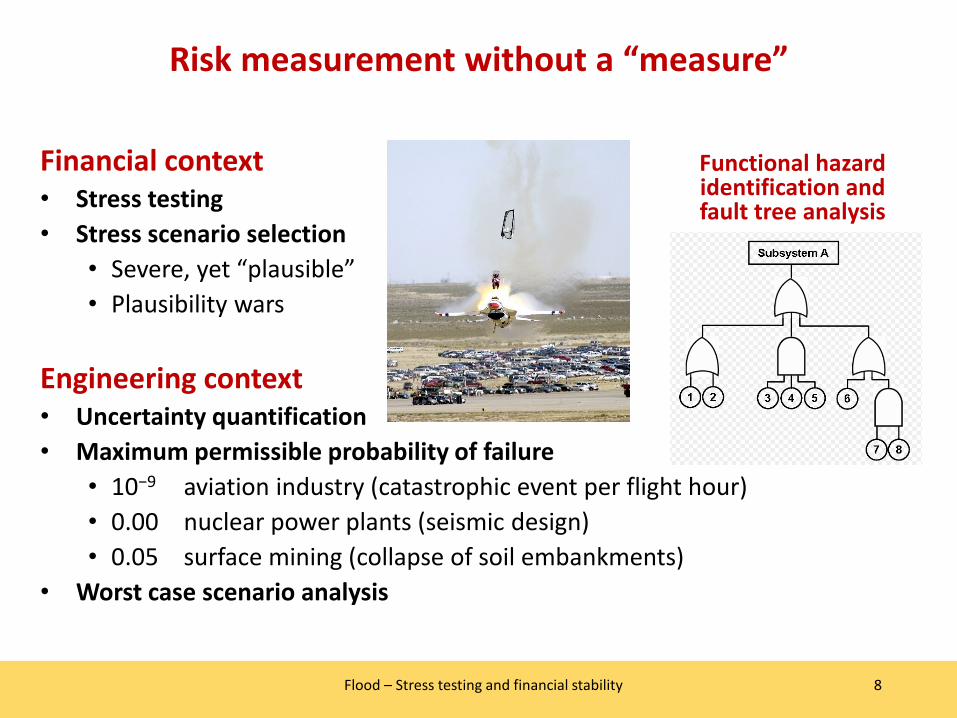
Risk measurement without a “measure”

8Flood – Stress testing and financial stability

Financial context• Stress testing• Stress scenario selection

• Severe, yet “plausible” • Plausibility wars

Engineering context• Uncertainty quantification• Maximum permissible probability of failure

• 10−9 aviation industry (catastrophic event per flight hour)• 0.00 nuclear power plants (seismic design)• 0.05 surface mining (collapse of soil embankments)

• Worst case scenario analysis

Functional hazard identification and fault tree analysis

Optimal Uncertainty Quantification (OUQ)

9Flood – Stress testing and financial stability

The Certification Problem• Guarantee that

P{G(X) ≥ α } ≤ εWhere• X is a risky or uncertain scenario• P is a probability measure• G(X) is a system response

(the “quantity of interest”)• G(X) ≥ α is some event

(typically undesirable)But• P is unknown or partially known• G is unknown or partially known

Optimal Uncertainty Quantification (OUQ)

10Flood – Stress testing and financial stability

SCAP as Certification

Ben Bernanke (2013)

Stress testing banks: What have we learned?

“In retrospect, the SCAP stands out for me as one of the critical turning points in the financial crisis. It provided anxious investors with something they craved: credible information about prospective losses at banks. Supervisors' public disclosure of the stress test results helped restore confidence in the banking system and enabled its successful recapitalization.”

Concentration inequalities

11Flood – Stress testing and financial stability

Chebyshev’s Inequality• Let X be an integrable random

variable with finite mean, μ, and finite (non-zero) variance, σ2.

• Then

P{ |X – μ| ≥ kα } ≤ 1/k2McDiarmid’s InequalityIn bounding P{ G(X) ≥ α }, if:• The components of X are statistically

independent, and• The component-wise oscillations of G(X)

have finite diameter, • Then

P{ G(X) ≥ E[G(X)] + ε } ≤ exp[-2ε2/Δ2]• Where Δ2 is the “wiggle room” in G(X):

Δ2 ≡ Σmδ2m for the component-wise

oscillation bounds, δm

McDiarmid has two key assumptions

Concentration inequalities bound the difference between an RV and its mean by limiting the extent of possible variation in the RV.E.g., a finite diameter restriction.

Application to financial stress testing

12Flood – Stress testing and financial stability

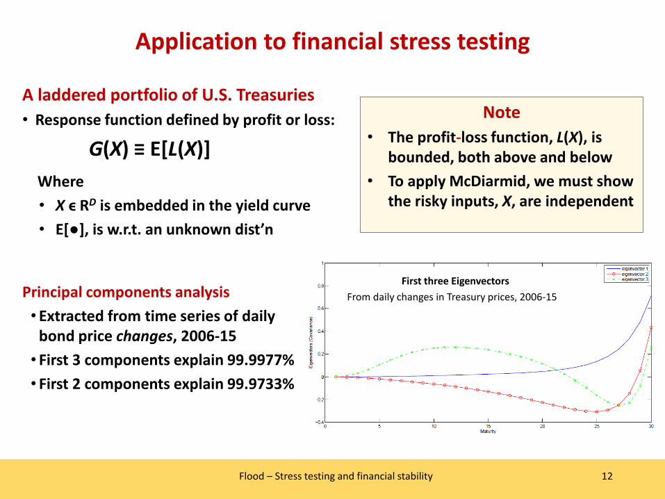
A laddered portfolio of U.S. Treasuries• Response function defined by profit or loss:

G(X) ≡ E[L(X)]Where• X ϵ RD is embedded in the yield curve• E[●], is w.r.t. an unknown dist’n

First three EigenvectorsFrom daily changes in Treasury prices, 2006-15

Note• The profit-loss function, L(X), is

bounded, both above and below• To apply McDiarmid, we must show

the risky inputs, X, are independent

Principal components analysis• Extracted from time series of daily

bond price changes, 2006-15• First 3 components explain 99.9977%• First 2 components explain 99.9733%

Results

13Flood – Stress testing and financial stability

Result #1 — Proof of Concept• We can implement OUQ for a simple financial stress test• McDiarmid’s distance allows for formal certification guarantees• McDiarmid is indeed stronger than Chebyshev

But this a limited case study• Static stress test, no policy response or human factors• Simple long-only portfolio, no optionality• Exploited a well-understood principal component analysis decomposition

Results

14Flood – Stress testing and financial stability

Result #2 – Formal measure of macroeconomic uncertainty• McDiarmid’s distance extracted from yield curve • Minimal assumptions required • Significant intertemporal variation• Peaks in 2009 (just when certification would be most valuable…)

Heterogeneity in macroprudential stress testing

15Flood – Stress testing and financial stability

What is a supervisory stress-test and what are its goals?

• Stress tests of individual FIs in isolation are microprudential stress tests

• Microprudential tests examine an FI’s viability • In several dimensions (capital, liquidity, etc.) • When the FI faces several general stress scenarios • And for institution-specific scenarios for the FI’s vulnerabilities

• A macroprudential stress test accounts explicitly for the systemic aspect and connection to the rest of the economy

• The macroprudential approach focuses on stability of the whole system

Heterogeneity in macroprudential stress tests

16Flood – Stress testing and financial stability

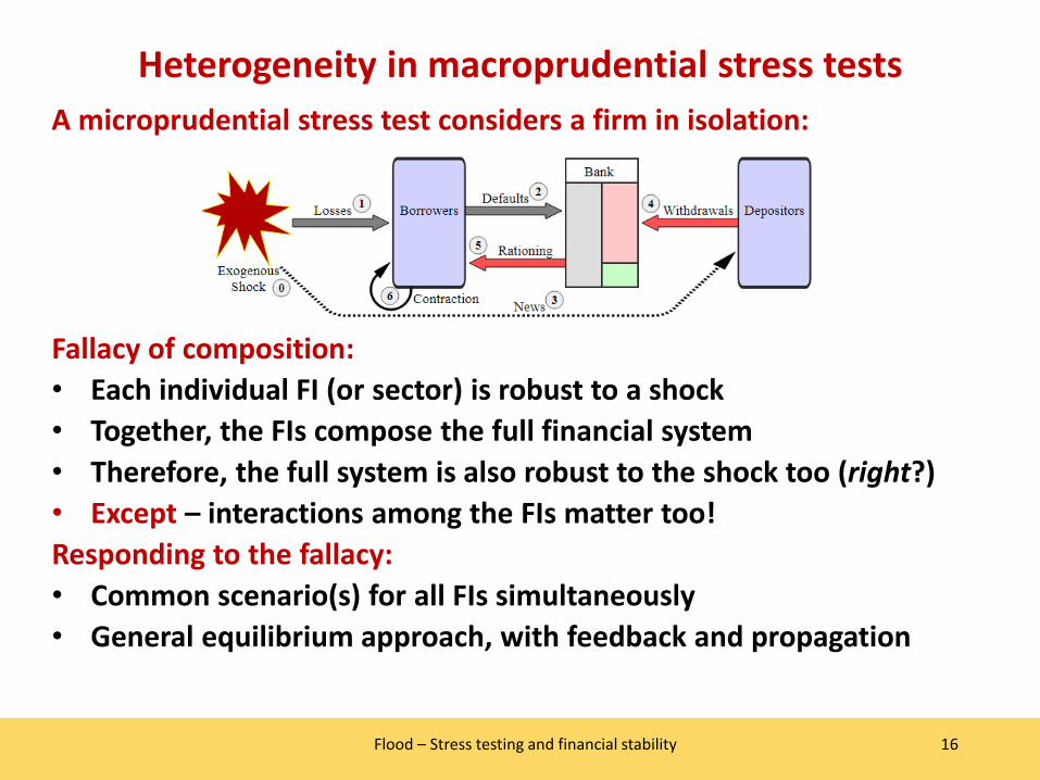
A microprudential stress test considers a firm in isolation:

Fallacy of composition:• Each individual FI (or sector) is robust to a shock• Together, the FIs compose the full financial system• Therefore, the full system is also robust to the shock too (right?)• Except – interactions among the FIs matter too!Responding to the fallacy:• Common scenario(s) for all FIs simultaneously• General equilibrium approach, with feedback and propagation

Heterogeneity in macroprudential stress tests

17Flood – Stress testing and financial stability

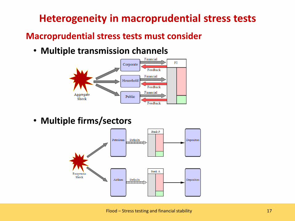
Macroprudential stress tests must consider• Multiple transmission channels

• Multiple firms/sectors

Importance of modeling heterogeneity

18Flood – Stress testing and financial stability

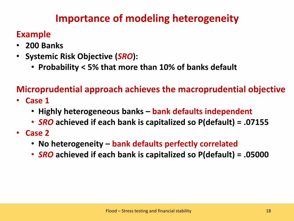
Example• 200 Banks• Systemic Risk Objective (SRO):

• Probability < 5% that more than 10% of banks default

Microprudential approach achieves the macroprudential objective• Case 1

• Highly heterogeneous banks – bank defaults independent• SRO achieved if each bank is capitalized so P(default) = .07155

• Case 2• No heterogeneity – bank defaults perfectly correlated• SRO achieved if each bank is capitalized so P(default) = .05000

Importance of modeling heterogeneity

19Flood – Stress testing and financial stability

Case 3 - Moderate heterogeneity: • Groups of FIs have similar risks

• 100 FIs lend primarily to airlines (default if oil prices are high)• 100 FIs lend primarily to oil companies (default if oil prices are low)

• SRO not achieved if each FI is capitalized as in Case 1 or Case 2

Num. defaults = �100 Prob = .07155 Poil high100 Prob = .07155 Poil low

0 Prob = 1–2(.07155) Poil moderate

• Instead, capitalize FIs so P(default) = .025 for high and low oil prices

Lessons1. Must account for heterogeneity to achieve the SRO2. Multiple scenarios may be needed to achieve the objective3. Extension should address hedging, feedback, and counterparty risk

Heterogeneity of stress responses

20Flood – Stress testing and financial stability

Example – Diverse portfolio responses to interest-rate shocks• Federal Home Loan Banks – identical mission: liquidity for mortgage lenders

• 12 institutions, regional scope• 2009 and 2010

• Duration of equity = (DA – DL) / Ve• Three parallel yield-curve shocks:

• – 200 bp (but ZLB)• Base case• + 200bp

Mostly upward-sloping• Except …

• Seattle 2010• Pittsburgh 2009• New York 2010• San Francisco 2010• Seattle 2009

A Game of Battleship

21Flood – Stress testing and financial stability

Forward stress test – McNeil and Smith (2010)

xLSLE ≡ arg min {g(x) : x ∈ S} for S ⊂ ℜd

• where LSLE = least solvent likely event (i.e., among x ∈ S)

CCAR / DFAST has three “likely events” (scenarios): • Baseline• Adverse• Severely adverse

Is three enough? • Non-monotonicity of payoffs• Anisotropy of payoffs• Model risk• Data limitations• Strategic behavior (e.g., window dressing)

Inverting the question

22Flood – Stress testing and financial stability

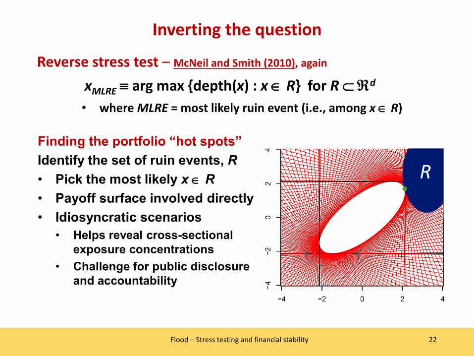
Reverse stress test – McNeil and Smith (2010), again

xMLRE ≡ arg max {depth(x) : x ∈ R} for R ⊂ℜd

• where MLRE = most likely ruin event (i.e., among x ∈ R)

Finding the portfolio “hot spots” Identify the set of ruin events, R• Pick the most likely x ∈ R• Payoff surface involved directly• Idiosyncratic scenarios

• Helps reveal cross-sectional exposure concentrations

• Challenge for public disclosure and accountability

R

Many dimensions of heterogeneity• Portfolio exposures (a.k.a. “business lines”)• Transmission channels

• Feedback• Propagation

• Diverse scenarios • Including behavioral challenges

Scenario design approach• Grid search to find the hot spots

• Arbitrary number of scenarios to cover possible “hot spots”• Focus on macroprudential hot spots

• Capitalize to minimize systemic risk

23Flood – Stress testing and financial stability

Applied reverse stress testing

Reading Suggestions• V. Acharya, R. Engle and D. Pierret (2014), “Testing macroprudential stress tests: The risk of regulatory risk

weights,” J. of Monetary Economics, 65, 36-53.• C. Aymanns, J. D. Farmer, A. Kleinnijenhuis and T. Wetzer (2018), “Models of Financial Stability and Their

Application in Stress Tests,” Ch. 6 in Hommes and LeBaron (eds.), Handbook of Computational Economics, Vol. 4: Heterogeneous Agent Modeling, North-Holland, 329-391.

• R. Bookstaber, J. Cetina, G. Feldberg, M. Flood and Glasserman (2014), “Stress Tests to Promote Financial Stability,” J. of Risk Management in Financial Institutions, 7(1), 16-25.

• J. Chen & M. Flood and R. Sowers (2017), “Measuring the unmeasurable: an application of uncertainty quantification to Treasury bond portfolios,” Quantitative Finance, 17(10), 1491-1507.

• M. Flannery, B. Hirtle and A. Kovner (2017), “Evaluating the information in the Federal Reserve stress tests,” J. of Financial Intermediation, 29, 1-18.

• M. Flood, J. Jones, M. Pritsker and A. Siddique (2019), “The Role of Heterogeneity in Macroprudential Stress Testing,” in: Farmer, Kleinnijenhuis, Schuermann and Wetzer (eds.), Handbook of Financial Stress Testing, forthcoming.

• M. Flood and G. Korenko (2015), “Systematic scenario selection: stress testing and the nature of uncertainty,” Quantitative Finance, 15(1), 43-59.

• B. Hirtle and A. Lehnert (2015), “Supervisory Stress Tests,” Annual Review of Financial Economics, 7, 339-355.• P. Kapinos, C. Martin and O. Mitnik (2015), “Stress testing banks: Whence and whither?” J. of Financial

Perspectives, forthcoming.• A. McNeil and A. Smith (2012), “Multivariate stress scenarios and solvency,” Insurance: Mathematics and

Economics, 50(3), 299-308.• T. Schuermann (2014), “Stress testing banks,” International J. of Forecasting, 30(3), 717-728.

24Flood – Stress testing and financial stability

Thanks!

25Flood – Stress testing and financial stability