
MARINE FISHERIES RESOURCE MANAGEMENT POTENTIAL FOR MACKEREL
65
P.O. Box 1390, Skulagata 4 120 Reykjavik, Iceland Final Project 2007 MARINE FISHERIES RESOURCE MANAGEMENT POTENTIAL FOR MACKEREL FISHERIES OF CAMBODIA EM Puthy Senior Officer Fisheries Administration Ministry of Agriculture Forestry and Fisheries Kingdom of Cambodia E-mail: [email protected] , [email protected] Supervisor Dr. Dadi Mar Kristofersson ([email protected] ) Department of Economics, University of Iceland ABSTRACT This paper estimates the maximum sustainable yield, virgin stock biomass and maximum economic yield of the mackerel fishery in Cambodia. Schaefer and Fox used the bio-economic, surplus production and biomass dynamic to determine the optimal utilisation of mackerel stocks. The estimated MSY is equal to 5,876 tonnes with an optimum level of effort corresponding to approximately 152 boats. The virgin stock biomass is at a level of 15,467 tonnes. The maximum profit and economic rents is estimated at US$ 2 million per annum. The paper examines alternative policies to reduce fishing effort in the inshore waters of Cambodia and improve the capacity of fishing vessels in offshore areas. The discussion emphasises initiating a cooperation policy between countries in the Gulf of Thailand for a cooperative management regime for the (residential) migratory species of mackerel. Therefore it is urgent to carry out a regional policy. Keywords: potential for mackerel fisheries of Cambodia, maximum sustainable yield.
Transcript of MARINE FISHERIES RESOURCE MANAGEMENT POTENTIAL FOR MACKEREL
PO Box 1390 Skulagata 4
120 Reykjavik Iceland Final Project 2007
MARINE FISHERIES RESOURCE MANAGEMENT
POTENTIAL FOR MACKEREL FISHERIES OF CAMBODIA
EM Puthy
Senior Officer
Fisheries Administration
Ministry of Agriculture Forestry and Fisheries
Kingdom of Cambodia
E-mail emputhyyahoocom drputhygmailcom
Supervisor
Dr Dadi Mar Kristofersson (dmkhiis)
Department of Economics University of Iceland
ABSTRACT
This paper estimates the maximum sustainable yield virgin stock biomass and
maximum economic yield of the mackerel fishery in Cambodia Schaefer and Fox
used the bio-economic surplus production and biomass dynamic to determine the
optimal utilisation of mackerel stocks The estimated MSY is equal to 5876 tonnes
with an optimum level of effort corresponding to approximately 152 boats The virgin
stock biomass is at a level of 15467 tonnes The maximum profit and economic rents
is estimated at US$ 2 million per annum The paper examines alternative policies to
reduce fishing effort in the inshore waters of Cambodia and improve the capacity of
fishing vessels in offshore areas The discussion emphasises initiating a cooperation
policy between countries in the Gulf of Thailand for a cooperative management
regime for the (residential) migratory species of mackerel Therefore it is urgent to
carry out a regional policy
Keywords potential for mackerel fisheries of Cambodia maximum sustainable yield
Em
UNU ndash Fisheries Training Programme 2
ACRONYMS
APIP - Agriculture Productivity Improvement Project
CFDO - Community Fishery Development Office
CPUE - Catch Per Unit Effort
DoF - Department of Fisheries
EEZ - Exclusive Economic Zone
FAO - Food and Agriculture Organization
FiA - Fisheries Administration
FJS - Fisheries Judicial System
FMR - Fisheries Management Regime
FMS - Fisheries Management System
GDP - Gross Domestic Production
hp - Horse power
HDR - Human Development Resource
IOs - International Organization
MAFF - Ministry of Agriculture Forestry and Fisheries
MCS - Monitoring Control amp Surveillance
MEY - Maximum Economic Yield
MoP - Ministry of Planning
MoT - Ministry of Tourism
MSY - Maximum Sustainable Yield
NACA - Network of Aquaculture Centres in Asia-Pacific
NGOs - Non-Governmental Organization
OSY - Optimum Sustainable Yield
PPP - Purchasing Power Parity
SEAFDEC - Southeast Asian Fisheries Development Centre
TAC - Total Allowable Catch
UNDP - United Nations Development Programme
USA - United State of America
US$ - United State Dollars
Em
UNU ndash Fisheries Training Programme 3
TABLE OF CONTENTS
1 INTRODUCTION 7
11 Problem statement 7
12 Objective of the study 7
13 Significance of the study 8
14 Organisation of the study 8
2 BACKGROUND 9
21 Country profile 9
22 Overview of the Cambodian marine fisheries sector 10
221 Marine catches 11
222 Catch by species and finfish production 11
223 Costal fishers and employment 13
224 Number of vessels 13
225 Annual contribution of marine fisheries to the economy 14
226 Fisheries landing ports 14
23 Mackerel fisheries 15
231 Mackerel production 15
232 Mackerel fisheries exploitation and its catch effort in Cambodia 15
233 Mackerel fish processing products 16
234 Marketing and price of mackerels 16
24 Marine fisheries resources management in Cambodia 18
241 Law and regulation 18
242 Management and administration 18
3 THE PRINCIPLES OF FISHERIES MANAGEMENT 19
31 The fisheries management system (FMS) 20
32 Monitoring control and surveillance (MCS) 22
33 Fisheries judicial system (FJS) 23
4 MODELLING 24
41 The biomass growth function 24
42 The harvesting function 26
43 The cost function 26
44 The complete model 27
45 Sustainable yield 27
46 Maximum sustainable yield (MSY) 28
461 Surplus production models 29
Em
UNU ndash Fisheries Training Programme 4
462 Biomass dynamic models 30
463 Specifying priors 31
5 ESTIMATION OF MODEL 31
51 Data sources 31
52 Parameter estimation 34
521 Maximum sustainable yield (MSY) 34
522 Virgin stock biomass (Xmax) 36
523 The schooling parameter (b) 37
524 Alpha and beta parameter (α) 37
525 Landings in base year t y(t) 37
526 Price of landings in base year t p(t) 37
527 Fixed cost ratio in base year eps(t) 38
528 Fishing effort in base year 38
529 Profit in base year (π) 38
53 Assumption and estimation 39
54 Empirical results 40
55 Model simulation and results 41
6 OPTIMUM SUSTAINABLE YIELD AND FISHERIES ECONOMICS 43
61 Maximum sustainable yield of mackerel fishery and current catches 43
62 Maximum economic yield 44
63 Sensitivity analysis of optimal fisheries policy 46
7 DISCUSSION 48
8 CONCLUSION 49
Em
UNU ndash Fisheries Training Programme 5
LIST OF FIGURES
Figure 1 Map of Cambodia 10
Figure 2 Map of the coastal areas of Cambodia 10
Figure 3 Number of marine fishing vessel from 2000-2006 (FiA 2007) 14
Figure 4 Volume of mackerel caught in the Gulf of Thailand from 1950-2004 (Sea
Around Us 2005) 15
Figure 5 Price of mackerels at landing and market site for 9 months in 2006 (FiA
2007) 17
Figure 6 Fisheries management systems a classification (adapted from lecture notes
UNU-FTP 2007 introduced by professor Arnason) 20
Figure 7 Illustrates the logistic biomass growth model G(x) 26
Figure 8 Illustrates the Fox biomass growth model G(x) 26
Figure 9 CUSUM plot of Schaefer model Figure 10 CUSUM plot of Fox model
34
Figure 11 The fishery in biomass-yield (biomass growth harvest) space for the
logistic distribution 42
Figure 12 The fishery in biomass-yield (biomass growth harvest) space for the Fox
distribution 42
Figure 13 Maximum sustainable yield and actual catches 44
Figure 14 Schaefer curve of relationship between revenue costs and effort 45
Figure 15 Fox curve of relationship between revenue cost and effort 46
Figure 16 Sensitivity analysis Schaefer chart of mackerel fisheries in Cambodia 47
Figure 17 Sensitivity analysis Fox chart of mackerel fisheries in Cambodia 47
Em
UNU ndash Fisheries Training Programme 6
LIST OF TABLES
Table 1 Demographic geographic and economic information for Cambodia (MoP
2006) 9
Table 2 Total fishery production inland and marine fishery from 2000-2006 (FiA
2007) 11
Table 3 Statistics of marine fisheries caught by groups in Cambodian coastal waters
(in tonnes) (Try et al 2006 and FiA 2007) 12
Table 4 Statistics of marine product of four main coastal areas 2006 (FiA 2007) 12
Table 5 Statistics of fishers and processors 1999-2006 (DoF‟s Statistics 2000-2006)
13
Table 6 Volume caught fishing effort and CPUE of mackerel from 1990-2006 (FiA
2007) 16
Table 7 The calculation procedure for estimating the MSY and fMSY by the Schaefer
model and by the Fox model using catch and effort data from 1992-2006 of the EEZ
of Cambodia 35
Table 8 Estimates of r and K at different levels of assumptions of growth coefficient
(k) of Rastrelliger brachysoma in the Gulf of Thailand 36
Table 9 Cost of fishery economic inputs 39
Table 10 The assumed mackerel fishery biological and fisheries parameters necessary
for calculating the unknown estimates 39
Table 11 Main results from estimations of the mackerel fisheries 41
Table 12 Sensitivity analysis of optimal mackerel fisheries policy 47
LIST OF APPENDICES
Appendix 1 Cost calculation of marine fishing operating in Cambodia 2006 55
Appendix 2 Use GRETL checking the parameter stability (intercept and slope) 55
Appendix 3 Summary output of model 60
Appendix 4 Summary result from Excel Spreadsheet 62
Appendix 5 Schaefer model estimates the sustainable fishery 63
Appendix 6 Fox model estimates the sustainable fishery 64
Em
UNU ndash Fisheries Training Programme 7
1 INTRODUCTION
11 Problem statement
The rapid expansion of fisheries in the Gulf of Thailand as well as in Cambodia has
raised considerable economic and environmental concerns about their management
Modern technology has increased fishing capacity resulting in the decline of the
resources and operations have become less profitable This manifests itself in the
increasing proportion of undersized fish and decreasing volume of commercially
important species in the Gulf Mackerel species are commercially valuable fish in the
Gulf and contribute significantly to the marine fish production of most countries
sharing the Gulf Since the introduction of trawling gillnets driftnets and purse seines
in the 1960s the total landing of mackerel in the Gulf of Thailand increased and a
peak production of around 140000 tonnes was reached in 1968 Subsequently
catches gradually declined to the lowest level of 6000 tonnes in 1978 (Sea Around Us
2005)
In Cambodia where the major fishing effort is directed at the exploitation of these
species they have been subjected to increasing exploitation A substantial effort is
made to improve landing records and assess the status of the species for management
purposes However for neighbouring countries which have established fisheries for
these species even primary estimates are not available and exploitation continues
without any knowledge of the trend
Nowadays these species play an important role for the marine fisheries sector not
only in Cambodia but also countries in the Gulf They affect the fishermen as well as
the local population whose income relies on revenues from fishing In general the
resources of the Gulf have declined due to over exploitation However mackerel is a
migratory species so local situations do not necessarily reflect the overall
development Landings of marine products in Cambodia have gradually increased in
recent years Particularly landings of mackerel species have increased from roughly
1000 tonnes in the 1990s to over 4000 tonnes in the 2000s (FiA 2007) Due to
relative stock abundance in Cambodian waters other countries such as Thailand and
Vietnam are major participants in the fishing in Cambodian waters On the other
hand the capacity of the Cambodian offshore fishing fleet is small compared to the
possible stock exploitation A significant increase in Cambodian fishing and landings
is possible by stricter regulations and monitoring of foreign fishing vessels
12 Objective of the study
The objective for this study is to determine the biological and economic potential for
the mackerel fishery in Cambodian waters by estimating biomass optimum
sustainable yield (OSY) and virgin biomass The estimation of maximum economic
and sustainable yield (MEY-MSY) is based on the steady-state relationship between
resource stock size fishing effort and yield adapted from Schaefer (1957) and Fox
(1970) (Arnason R and Bjordal T 1991) This methodology is widely known as bio-
economic modelling It is a commonly used surplus production model for multi-
species fisheries in the tropics This approach outlines the effects of policy and
management systems for fisheries economic growth
Em
UNU ndash Fisheries Training Programme 8
The purpose of this study is to provide a current bio-economic analysis of the
mackerel fishery in Cambodian waters and to estimate both economic and biological
maximum levels of yield and effort given the nature of the fishery and the lack of
joint management of the resource with other nations in the Gulf of Thailand
Corresponding measures to manage the mackerel species in Cambodia will be
discussed as well as implications for the management of the stock in the whole of the
Gulf This study attempts to put together available information from the fisheries to
assess the current situation and to express views that are likely to stimulate further
investigations to better understand and manage the resources
13 Significance of the study
FAO (1999) indicates that the Gulf of Thailand is among the most productive fishing
grounds in the world and APIP (2001b) states that Cambodia‟s coastal area is the
most productive in the Gulf (Gillett R 2004) In fact the total volumes of
Cambodia‟s catches in the Gulf are probably low and low per unit compared to
Thailand and Vietnam The marine fishery of Cambodia is multi-species and the
main commercial species include mackerels scads anchovies and snappers which
are exploited from September to January
Mackerels are coastal pelagic fish which include short mackerel Indian mackerel
island mackerel and king mackerel exploited in the late 1940s At present driftnets
purse seines and gillnets are common gears which fishermen use to catch mackerel
These fish have been caught mostly by Cambodia Malaysia Thailand and Vietnam
from the Gulf of Thailand However situations of biomass growth stock size and
environmental carrying capacity for mackerel species are not available
Hopefully this study will provide recommendations on sustainable biomass growth
sustainable harvesting and optimum fishing effort as well as suggestions on the
necessary adjustments to policy in the marine fisheries sector in order to increase
catchability and improve the management system of production This is of great
importance to the fisheries administration fishermen associations and the current
operation and management system
14 Organisation of the study
The organisation of this paper is as follow Chapter 2 provides a background the
marine fisheries and the management system Chapter 3 reviews the principles of
fisheries management Chapter 4 summarises the bio-economic model ndash the Gordon
Schaefer model used to predict or estimates of maximum sustainable yield and
optimal sustainable yield of mackerel fisheries The data and results of estimation are
presented in chapter 5 Chapter 6 discusses of optimum sustainable yield and fisheries
economics Chapter 7 discusses fisheries issues and Chapter 8 provides conclusion
and recommendations to outline policy for Cambodian marine fishery sector and the
Gulf of Thailand
Em
UNU ndash Fisheries Training Programme 9
2 BACKGROUND
21 Country profile
Cambodia is a tropical country located in Southeast Asia well known for its rich
natural resources especially in forestry and fisheries These resources play an
important role in the national economy Agriculture is the main contributor to the
national economy Rice and fish products have been considered as the major means of
generating food The agricultural sector including rice farming livestock fisheries
forestry and cultivation of other cash crops provides direct employment to 706
percent of Cambodia‟s labour force Its share of the GDP decreased from some 452
percent in 1998 to 351 percent in 2005 (MoP 2006) The GDP in 2005 was about
US$ 350 per capita which places Cambodia as one of the poorest countries in the
world where the daily income is less than US$ 1 (Table 1) Cambodia is ranked 131
out of 177 countries in achievement made in human development with a GDP per
capita (Purchasing Power Parity) of US$ 2727 (UNDP-HDR 20072008)
Table 1 Demographic geographic and economic information for Cambodia (MoP
2006) Total geographical area 181035 km
2
Population 137 million in 2005
Annual population growth rate 181 in 2005
Share of rural population 85 in 2005
Labour force 10 years and above 75 million in 2004
Share in employment (2004)
Agriculture 351
Industry 263
Service 386 (2006 est)
Per capita GDP (US$) 350 in 2005
Annual GDP growth rate (constant prices) 7 in 2005
Agriculture Forestry and Fisheries
Key indicator Unit 1993 2000 2005
Estimates
2010
Projected
Annual GDP (constant prices) Billion riels 8494 14089 19294 25747
Share of GDP
Paddy amp crops
188
165
142
127
Livestock and poultry 89 54 46 43
Fisheries 136 108 93 8
Forestry 43 33 2 16
Em
UNU ndash Fisheries Training Programme 10
Figure 1 Map of Cambodia
22 Overview of the Cambodian marine fisheries sector
The marine fish stocks are a heavily exploited resource due to the high density of the
coastal population around the Gulf of Thailand Cambodia has a marine coastline of
435 km which covers two cities and two provinces The Exclusive Economic Zone
(EEZ) covers approximately 55600 km2 and is relatively shallow with an average
depth of about 50 m The marine fishing grounds are located on the eastern bank of
the Gulf of Thailand There are 525 species of marine finfish 20 species of marine
crabs 42 species of marine gastropods 24 species of marine bivalves and 11 species
of marine mammals (Tana 1997 Try 2003) Marine fisheries development has been
slow compared to the inland fisheries which are yielding approximately 400000
tonnes of fish annually The landed catch of marine fisheries was estimated at around
60000 tonnes in 2006 (FiA 2007)
Figure 2 Map of the coastal areas of Cambodia
Em
UNU ndash Fisheries Training Programme 11
221 Marine catches
The Department of Fisheries statistics (2004) cited by the Community Fishery
Development Office (CFDO 2005) reports that the annual marine catches were
estimated at about 36000 tonnes in 1994 ndash 2000 This number excludes the catches of
subsistence and illegal foreign fishing The Fisheries Administration has estimated the
increase in fish production from 36000 tonnes in 2000 to 60500 tonnes in 2006
(Table 2) which includes catch in mangrove areas due to the fact that the harvest of
mangroves is covered by the present fisheries law
In fact the actual catch of marine fisheries is higher than the official statistics suggest
This is because the catches from subsistence fishing including family-scale fisheries
are largely unrecorded Furthermore catches from illegal fishing activities are not
recorded Csavas et al (1994) state that information on the landing of marine fish in
Cambodia can be inferred from records of fish landings from the Thai portion of the
Gulf of Thailand This is partly due to the Thai vessels fishing in Cambodian waters
and some Cambodian fishing boats selling or transferring their catch to Thai mother-
vessels at sea or landing in Thai ports According to the DoF internal reports catches
from licensed Thai vessels in Cambodian water are estimated to be from 26500
tonnes to 37500 tonnes (Gillett 2004) Robert (Gillett R 2004) also concluded that if
this is indeed the case this amount would approach the total marine catch recorded for
all Cambodian fishing vessels operating offshore Substantial Thai catches in
Cambodian waters complicate any management strategy for Cambodian fish resources
because of difficulties associated with ensuring that rents from improved Cambodian
management actually benefit Cambodian fishermen and not only the less regulated
Thai fishing fleet
The marine fishery involves coastal fishers in inshore areas and foreign fishers
operating legally and illegally in offshore areas (NACA 2004) Cambodia currently
does not have the capacity to exploit offshore areas Since 1992 marine fisheries
statistics have included estimates of catches by foreign fishers licensed to operate in
the EEZ of Cambodia (DoF 2001d)
Table 2 Total fishery production inland and marine fishery from 2000-2006 (FiA
2007)
Year Total
(tonnes)
Inland (ton) Marine
(tonnes) Total Commercial
fisheries
Familysubsist
ence fisheries
Rice field
fisheries
2000 281600 245600 85600 110000 50000 36000
2001 427000 385000 135000 140000 110000 42000
2002 406150 360300 110300 140000 110000 45850
2003 363500 308750 94750 120000 94000 54750
2004 305800 250000 68100 106400 75500 55800
2005 384000 324000 94500 137700 91800 60000
2006 482500 422000 139000 181000 102000 60500
222 Catch by species and finfish production
Finfish is the main group of annual total catches by year (Table 3) Try (2003)
indicated that 33 species of finfish are commonly exploited Only five species are
very abundant in the landings Megalaspis cordyla (torpedo scad) Scomberomorus
commersoni (narrowbarred Spanish mackerel) Rastrelliger brachysoma (short
Em
UNU ndash Fisheries Training Programme 12
mackerel) Rastrelliger kanagurta (Indian mackerel) and Atule mate (yellowtail scad)
The volume of finfish caught in 2006 decreased slightly compared to 2005 but the
total catches have increased in 2006 as Anadromous fish (3678 tonnes) were not
record in 2005
The catches of trash fish each year rank the second after finfish (Table 3) In 1960 the
trawl gear was introduced to fishers in Cambodia that allows for catch of demersal
fish and juveniles During the past three decades trash fish was discarded due to no
demand and no value in the market But after 1993 a factory was built in Sihanoukvill
for processing trash fish for fish feed Therefore fishers catch and collect the trash
fish resulting in that the volume of trash fish has recently increased
As the market price of economic fishes has gradually been increasing trash fish have
become food for local people and particularly the poor coastal dwellers who have a
low income According to Try (2006) it was estimated that the trash fish caught by
trawl in 1980 is about 30-40 of the total catch but the percentage of trash fish was
recently increased probably to 60-65 of marine fish catches by trawl It seems that
to be encouraging the fishers use a more efficient gear to fish in inshore waters than
offshore Perhaps they are also using illegal fishing gears such as trawlers mosquito
net push and small mesh sizes of nets catching all fish species and sizes The marine
fish catches in 2006 have declined for all groups except shrimp from 2005 (Table 3)
Table 3 Statistics of marine fisheries caught by groups in Cambodian coastal waters
(in tonnes) (Try et al 2006 and FiA 2007)
Yea
r
Fin
fish
Tra
sh f
ish
Sh
rim
p
pra
wn
s
Ray
s
Sq
uid
cutt
lefi
sh
Lo
bst
ers
Cra
bs
Gas
tro
po
ds
Sea
slu
g
An
adro
mo
us
fish
To
tal
mar
ine
fish
ery
2000 15526 9833 2905 245 2627 59 3593 801 11 410 36010
2001 16873 10847 3872 209 2355 40 3462 3681 0 661 42000
2002 18910 11752 3827 553 2681 122 3545 3007 3 1410 45810
2003 26596 14859 4055 727 3577 169 4028 648 2 61 54722
2004 25639 16570 3824 620 2984 124 3458 2457 0 124 55800
2005 26141 18265 4124 996 3723 1233 4301 1215 2 0 60000
2006 25641 17194 4778 476 3551 115 4180 897 0 3678 60500
Almost 90 of the marine fisheries production in Cambodia is from two coastal
provinces Sihanoukvill and Koh Kong (Table 4) The total catches of finfish are
mackerel fish amount 4650 tonnes (FiA 2007) The trash fish is second in rank
among the group species caught of which Koh Kong and Sihanoukvill rank at the top
Table 4 Statistics of marine product of four main coastal areas 2006 (FiA 2007)
Cit
y
pro
vin
ce
Fin
fish
Tra
sh f
ish
Sh
rim
p
pra
wn
s
Ray
s
Sq
uid
cutt
lefi
sh
Lo
bst
ers
Cra
bs
Gas
tro
po
ds
An
adro
mo
us
fish
To
tal
mar
ine
fish
erie
s
Kampot 2103 1674 386 32 130 5 635 415 2000 7380
Kep 300 - 35 5 10 - 45 17 18 430
Koh Kong 13519 10500 1622 89 1100 - 2000 280 160 29270
Sihanoukvill 9709 5020 2735 350 2311 110 1500 185 1500 23420
Total 25631 17194 4778 476 3551 115 4180 897 3678 60500
Em
UNU ndash Fisheries Training Programme 13
223 Costal fishers and employment
Most coastal fishers are poor and generally use small-scale fishing gear that is only
adequate for use inshore and in mangroves There are limited numbers of coastal
fishers that have sufficient capital to invest in the necessary vessels and gear for
offshore fishing The capacity of fishers fishing offshore in the EEZ is not large
compared to the potential exploitation
Officially the statistics of fisheries employment have shown only the number of
people involved in fisheries harvesting processing and culturing There are no
statistics on other numbers of people employed in fisheries related activities The
number of fishers and the number of fish processor is reflected in Table 5 below
Table 5 Statistics of fishers and processors 1999-2006 (DoF‟s Statistics 2000-2006) Year Harvesting labour force in marine sector
Processing labour
force Familyrice field
Mobileartisanal
Fisheries Total fishers
No of
families
No of
fishers
No of
families
No of
fishers
No of
families
No of
fishers
No of
families
No of
processors
1999 0 0 3910 11721 3910 11721 373 1527
2000 0 0 6557 14647 6557 14647 379 1631
2001 6445 8067 4137 15350 10582 23417 370 1499
2002 24818 45940 9648 26130 34466 72070 1472 2379
2003 16047 28638 13159 40014 29206 68652 990 1815
2004 16475 31657 10865 33274 27340 64931 1407 4234
2005 - - - - - - - -
2006 18949 37990 12006 36582 30955 74572 1226 29412
224 Number of vessels
Non-motorised and motorised vessels are used in Cambodia‟s marine fisheries Most
non-motorised vessels are used by the small-scale fishers who carry out subsistence
fishing The Fisheries Department has statistically categorised the non-motorised
vessels based on their dead weight The three categories are less than 5 tonnes more
than 5 tonnes and Duk-boats but the Duk-boat is not directly used for fishing (ie it
is used for transporting the fisheries products)
The motorised vessels are divided into four categories based on engine power less
than 10 hp 10 to 30 hp 30 to 50 hp and more than 50 hp This classification does not
include data on the number of vessels involved in small-scale and large-scale
fisheries
The number of non-motorised vessel in 2000 was only 255 and increased to 841 boats
in 2002 operating within Cambodia‟s coastal zone then it dropped dramatically to
272 boats in 2004 and increased again to 821 boats in 2005 and 1059 boats in 2006 as
illustrated in Figure 3
Noticeably the number of motorised fishing vessels seems to increase linearly from
5037 boats in 2000 to 7027 boats in 2005 and drop to 6236 boats in 2006 Most of
the motorised fishing vessels with large fishing gears are required to have licenses to
operate Two systems exist of motorised fishing vessels licenses one is a license
issued by the provincial fisheries office for all motorised vessels equipped with engine
Em
UNU ndash Fisheries Training Programme 14
power under 33 horse power (hp) and another is a license issued by the Fisheries
Administration for all motorised vessels equipped with an engine power above 33
horse power (hp)
Referring to regulations on offshore and inshore vessels it can be assumed that all the
motorised vessels which have small engine power (below 50 hp) and non-motorised
vessels operate inshore Motorised vessels equipped with engine power greater than
50 hp should operate offshore
Fishing vessels equipped with engine power higher than 50 hp may use a labour force
from 5 to 15 people depending on the fishing gear used For boats with an engine
power higher than 100 hp the labour force may be 15 to 30
Figure 3 Number of marine fishing vessel from 2000-2006 (FiA 2007)
225 Annual contribution of marine fisheries to the economy
According to a government report the marine capture fishery has increased from
36000 tonnes in 2000 to 60500 tonnes in 2006 (Table 2) Thus the average marine
capture fishery was around of 50700 tonnes per year from 2000 to 2006 Try et al
(2006) mentioned that the average market price of marine fish is US$ 1 per kg The
marine capture fishery can be estimated to value US$ 507 million a year at the
market site If the tourism industry in Cambodia shows a steady increase of 20
yearly (MoT 2007) the demand for food consumption for tourists will increase This
leads to an increase in the domestic market price of marine fish in Cambodia and the
marine capture fisheries in 2006 can be estimated to value in total revenue around
US$ 635 million According to Try et al (2006) the capture marine fishery values
account of US$ 15 million to US$ 30 million excluding the illegal export which is
un-reported This estimation was at the average market price of trashfish at 500
Cambodian Riels per kg The share of fisheries in the GDP or government revenue
was 108 in 2000 and the estimate for 2005 is 930 (Table 1)
226 Fisheries landing ports
Landing locations are not separated from fishing locations and harbour facilities are
limited Much of the catch is transferred to Thai vessels at sea for landing in Thailand
(FAO 2005) Landing sites of four main coastal areas are used for statistics a total of
about 131 locations landings exist in Sihanoukvill 69 Koh Kong 55 Kampot 4 and
Em
UNU ndash Fisheries Training Programme 15
Kep City 3 Most landing ports are small and rural services and facilities are poor It
may be concluded that fishery landing ports of four main coastal provinces are not of
interest to the private sector to invest in rather these are subsidised by the
government
23 Mackerel fisheries
Mackerel consists of commercial pelagic groups which include short mackerel Indian
mackerel Indo-Pacific mackerel Spanish mackerel and island mackerel They are the
most important pelagic species in the Gulf of Thailand harvested by commercial and
traditional gears The local name ldquoPlathu Kamongrdquo is used loosely to refer to all
these fish species
231 Mackerel production
The highest recorded annual landing of mackerel (Rastrelliger) was 139220 tonnes
and contributing 14 to all the marine fish landed in 1968 in the whole Gulf of
Thailand Second to this 122156 tonnes or 11 of the marine fisheries landings were
recorded in 1969 (Sea Around Us 2005) These species supported the purse seine and
gillnet fisheries since the early 1960s and have remained important until now In fact
mackerel is the most dominant commercial food fish in the Gulf of Thailand
The catch of mackerel declined from about 40000 tonnes in the 1950s to around 20000
tonnes in the 1980s An unusually sharp increase in catch occurred though in 1965-1971
when the catch reached 140000 tonnes The pressure from the industry in Thailand has
resulted in overexploitation Ahmed et al (2007) state that ldquofor a number of decades
fisheries development in the Gulf of Thailand has concentrated on increasing fishing
effort to maintain or increase the production volumerdquo Most important pelagic fish in
the Gulf of Thailand are fully exploited especially Indo-Pacific mackerel anchovies
round scad and sardines and demersal resource stocks are over-fished (FAO 1995)
Figure 4 Volume of mackerel caught in the Gulf of Thailand from 1950-2004 (Sea
Around Us 2005)
232 Mackerel fisheries exploitation and its catch effort in Cambodia
Mackerel is not only sold on the domestic market but is also exported to Thailand
every year both fresh and processed Mackerel in Cambodia is caught by artisanal
fishermen as well as the industrial fishery The artisanal fishery operates from small
Em
UNU ndash Fisheries Training Programme 16
boats with outboard engines of less than 33 hp Most of these fishing boats use
gillnets to catch in inshore areas The industrial mackerel fishery is operates offshore
using purse seines or driftnets with boat engines up to 50 hp The commercial fishing
boat can stay at sea fishing 2 to 5 days This type of boat has facilities to keep fish for
long time
Since 1990 the catch of mackerel by Cambodia had increased from about 1000
tonnes to 4650 tonnes in 2006 (Table 6) From 2002 to the present the catch has been
stable at around 4500 tonnes but the effort has increased with a corresponding
reduction in CPUE
The gillnet boats fish for mackerel approximately 25 days a month 8 months a year
The purse seine operates only during the dry season period of 5 months (20 days per
month) The purse seine boats have crews of about of 15 to 30 people The gillnet
boats can on the other hand operate with a labour force of only 2 to 3 people
Table 6 Volume caught fishing effort and CPUE of mackerel from 1990-2006 (FiA
2007)
Year
Catches
volume
(tonnes)
Fishing effort CPUE
(Kgperson
day)
Boat used gillnet Boat used purse seine Total
boat
Total
labour Boat Labour
(person) Boat
Labour
(person)
1990 1395 - - - - - - -
1991 1212 - - - - - - -
1992 1101 3 9 13 260 16 269 40
1993 1424 9 27 14 280 23 307 43
1994 1513 31 93 15 300 46 393 31
1995 1683 10 30 16 320 26 350 44
1996 1452 14 42 6 320 30 362 36
1997 1278 114 342 15 300 129 642 13
1998 1447 122 366 15 300 137 666 14
1999 1738 172 516 8 160 180 676 15
2000 1559 155 465 10 200 165 665 14
2001 1731 56 168 10 200 66 368 32
2002 4300 50 150 10 200 60 350 86
2003 4421 73 219 13 260 86 479 63
2004 4764 117 351 10 200 127 551 53
2005 4906 250 750 4 80 254 830 31
2006 4650 181 543 6 120 187 663 39
233 Mackerel fish processing products
The mackerel in Cambodia is traditionally processes by salted or steaming For
steamed fish ldquoshort body mackerelrdquo is the local name called as Trey Chom Houy but
for salting ldquoSpanish mackerelrdquo is used the local name is Trey Borb Most production
is for the domestic market Data is limited on export
234 Marketing and price of mackerels
Locally the price of mackerel and its products can be different between markets
throughout the land However the difference between the markets of the four
Cambodian coastal areas is small The Sihanoukville market site is the main
Em
UNU ndash Fisheries Training Programme 17
distribution centre of marine fisheries products into the local market thus the market
price of Mackerel fishes and its products in Sihanoukvill can be assumed as the local
market standard price of Mackerel fishes and its products According to monthly
reports of the Marine Fishery Division the price of mackerel at the landing site and
domestic market is actually increasing especially in the wet season when catch is
small and but demand is high
In 2006 the price of short mackerel at the landing site from January to September
fluctuated from US$ 450 to US$ 625 per tonne1 (Figure 5) Based on data estimated
by the Fishery Administration the landing volume of mackerel species in 2006 was
about 4650 tonnes and can be estimated at around US$ 252 million or 4 of the
marine fishery revenue in 2006 Spanish mackerel is selling at a high price at the
landing and market site but the landing volume is small compared to short mackerel
The landing price of Spanish mackerel within a 9 month period in the year 2006
fluctuated increasingly from US$ 1375 to US$ 3500 per tonne Figure 5 illustrates
the price of short mackerel and Spanish mackerel correlated at two sites domestic
market and local landing site
In general the price of marine fish at landing as well as market site has increased over
the years due to an increase in the fishing operational cost Moreover increased
population leads to high market demand for human consumption whereas the natural
resources are gradually decreasing Thuok et al (2001) stated that marketing channels for
marine products are not so well developed for food security and economy reasons it is
believed that emphasis should be placed by the administration in support of the private sector
on the development and enhancement of marketing of marine fishery products
Figure 5 Price of mackerels at landing and market site for 9 months in 2006 (FiA
2007)
1 The price of mackerel at landing site was conducted and reported to the Fishery Administration by Marine
Fishery Division from January to September in 2006
Em
UNU ndash Fisheries Training Programme 18
24 Marine fisheries resources management in Cambodia
241 Law and regulation
The Cambodian marine fishery is managed under the Fisheries Law of 2006 which is
an improved and updated version of the law from 1987 The main objective of the law
and regulation is to manage and conserve the marine fishery resources in a sustainable
manner Additional objectives are to generate governmental revenue improve the
livelihood of local communities and achieve ecologically sound management by an
improved statistical system gear restrictions area limitations and time closures
Management objectives other than those in the Fishery Law 2006 exist and are
attained by the Ministry of Agriculture Forestry and Fishery (proclaim issue) ie
closed season from 15 January to 31 March for mackerel species
For management purposes the marine fisheries are divided into two groups
Coastal fisheries small family-scale fishing operating in fishing zone 1 which
extends from the coast to a depth of 20 m this fishing zone was almost managed by
community fisheries The coastal community fisheries were established after the
government recognised the poor management of the fisheries sector which resulted in
a movement for reform in 2000 Nowadays 40 community fisheries have been
established along the coast to encourage coastal dwellers to participate in the
management of their resources Fishers use boats without engines or with engines of
less than 50 hp Licenses are not required for boats with no engine or with engines
below 33 hp but for boats with more than 33 hp engines a license fee of 27000 Riels
(US$ 7) per horsepower per year is required Fishing activities are not allowed to
include other fishing gears such as trawls or light fishing
Commercial fisheries refer to large-scale fishing from 20 m depths to the limits of the
EEZ Boats used have engines with more than 50 hp which must be licensed for a fee
of 27000 Riels (US$ 7) per horsepower per year Prohibited fishing gears and
methods include pair trawling light fishing and other illegal fishing gears All marine
fisheries are open year round apart from mackerel for which fishing is banned from
15 January to 31 March (DoF 2001d) Most of the small boats (engine lt 50 hp)
marine fishing fleets use alternative multi-fishing practices following the seasonal
appearance of marine resources including purse-seines gill nets push nets and
trawling Foreign poachers use prohibited gears such as large bottom trawls long drift
nets pair trawlers light fishing and explosives (DoF 2001d)
242 Management and administration
Despite a few limitations on the fisheries in the Gulf of Thailand fisheries there fall
under the framework of unregulated open access In addition there are no limits
placed on the amount of gears that can be used the amount of time that can be spent
fishing or on the quantity of fish that may be captured
Generally coastal fishers can operate all year round by using many different types of
fishing gears However the use of fishing gears is dependent on a number of critical
factors including (1) the capital invested (2) experience and traditions of the fishing
communities in different locations along the coast (3) seasonal abundance of different
Em
UNU ndash Fisheries Training Programme 19
species (4) seasonal weather conditions and (5) ecological conditions associated with
the fishing grounds (eg inshore offshore mangrove coral reef etc)
Fishing in offshore areas is still a challenge and there is a lack of strong law
enforcement measures against illegal fishing from neighbouring countries It is a
problem represented in the low annual production of marine fisheries The present
management of data collection is not sufficient to develop plans for scientific
management of marine fish stocks The lack of knowledge of fish biology ecology
and their dynamics results in a poor understanding of the recent changes in marine
fish stocks (MAFF-DoF 2004)
On the other hand the fisheries competency is still inadequate This is true in terms of
inspection specialists and the lack of adequate physical means to enforce legislation
such as protection against illegal fishing (ie the Fisheries Administration is less able
to set up or install the right technology a high speed boat radio communication and
other facilities for coast guard operations) Furthermore in the 1990s the political
environment was unstable which affected the business environment and led to less
investment capital
However the government and Fisheries Administration have overcome many
obstacles to develop and manage marine fisheries resources as well as the fisheries
sector in the past years Especially a recent achievement is the Fishery Law
completely promulgated public using in 2006 (FiA 2007) The new law was updated
from the previous Fishery Law of 1987 which was based on legislation from 1956
1958 and 1960 (revised) The updated law was also drafted with participation from
stakeholders IOs NGOs and relevant partners through research study and sustainable
development projects on the fisheries sector framework In terms of gains marine
production through fishing effort as well as improve capacity of fishing and biomass
management in EEZ
3 THE PRINCIPLES OF FISHERIES MANAGEMENT
This chapter has been adapted from the lecture notes in the UNU-FTP specialist
course on Fisheries Policy and Planning by Prof Ragnar Arnanon
The need for fisheries management stems fundamentally from the fact that fish
resources are common property It is well known both from theory and experience
that common property resources will be overexploited and possibly irreversibly
depleted unless subjected to appropriate fisheries management Essentially the
fisheries management regime is a set of social prescriptions and procedures that
control the fishing activity Similarly fisheries management requires either collective
action at the industry level or external usually government intervention
The principles of fisheries management or fisheries management regimes consist of i)
the fisheries management system (FMS) ii) monitoring control and surveillance
(MCS) and iii) fisheries judicial system (FJS) These three components of the
fisheries management regime are strongly interdependent All three components of the
fisheries management regime are crucial to its success They are links in the same
chain If one of them fails the fisheries management regime as a whole fails
Em
UNU ndash Fisheries Training Programme 20
31 The fisheries management system (FMS)
The fisheries management system specifies the regulatory framework for the fishing
activity It consists of all the rules that the fishing activity must obey such as gear and
area restrictions fishing licences catch quotas etc In many countries most fisheries
rules are based on explicit legislation In others they are primarily based on social
customs and conventions
The fisheries management system is basically a set of rules about how the fishery
should be conducted These rules may be formal ndash for instance in the form of
published laws and regulations ndash or they may be informal ndash a part of the social culture
governing fishing behaviour In most fisheries both types of fisheries management
rules the formal and the informal apply The purpose of the fisheries management
system is to contribute to the generation of net economic benefits flowing from the
fishery
The fisheries management represents the application of specific fisheries management
instruments or tools Typical fisheries management tools are for instance fishing gear
restrictions limitations on the number of allowable fishing days during the year area
closures and so on Thus the fisheries management tools are like variables or more
precisely control variables and the fisheries management measures the values that can
be chosen for these control variables
Now fisheries management systems consist of particular combinations of one or more
of these tools Thus obviously the number of possible fisheries management systems
increases very fast with the number of available fisheries management systems Most
of them may however be grouped into two broad classes i) Direct fisheries
management and ii) indirect fisheries management as illustrated in Figure 6
Figure 6 Fisheries management systems a classification (adapted from lecture notes
UNU-FTP 2007 introduced by professor Arnason)
Direct fisheries management attempts to control the components of the fishing
activity directly by commands or more often restrictions that must be adhered to
Indirect economic fisheries management by contrast attempts to induce the fishing
firms to behave differently by modifying the operating conditions of the fishery
without imposing direct constraints The difference between direct biological and
economic fisheries management lies in what they seek to control Direct biological
fisheries management attempts to alter the biological yield of the fishery Thus under
biological fisheries management for instance the sustainable yield curve is normally
shifted Direct economic fisheries management attempts to alter the behaviour of the
Em
UNU ndash Fisheries Training Programme 21
fishing firm days vessel size etc Thus direct economic management generally
affects the cost structure of the fishery directly
Indirect fisheries management alters the operating conditions of the fishing industry
There are of course many ways to do this Most however belong to two main
categories (a) taxes (and subsidies) which basically alter the prices facing the fishing
industry and (b) property rights which alter the nature of the external effects imposed
by the fishing firm on one another
Most fisheries management tools are fall quite naturally into one of the fisheries
management categories in Figure 6 The main exception is the total harvesting
restriction or total allowable catch (TAC) Of all the fisheries management systems
considered above only (i) certain property right arrangements and (ii) tax on catch
seem to be theoretically capable of delivering the full potential economic benefits of
fisheries Direct fisheries management irrespective of whether it is based on
biological or economic restrictions seems particularly inept for this purpose
Em
UNU ndash Fisheries Training Programme 22
32 Monitoring control and surveillance (MCS)
The primary task of the monitoring control and surveillance system is to observe the
fishing industry‟s activities and to enforce its adherence to the rules of the fisheries
management system Its secondary but nevertheless very important task is to collect
data about the fishery that can be used to improve both the fisheries management and
fisheries judicial system as well as the monitoring control and surveillance system
itself Broadly speaking the phrase refers to two activities i) the monitoring of the
fishery and the activities of the fishing (harvesting) industry and ii) the enforcement
of fisheries management rules
MCS is as already discussed a crucial component of any fisheries management
regime Logically it is the management authority that must conduct and co-ordinate
the MCS activity although it may engage contractors it is the central fisheries
manager ie the government that operates the MCS activity
The monitoring part of MCS involves collection of the relevant biological data about
the fish stocks and the surrounding ecosystem as well as the relevant technical
economic and behavioural data about the fishing industry and its activities The
monitoring activity is conducted for essentially two purposes i) to gather information
for improving the fisheries management ie data generation monitoring and ii) to
gather information for the purpose of enforcing existing fisheries management rules
ie enforcement monitoring It is important to realise that in order to transform
fisheries data into sensible decisions on fisheries management measures and
modifications of the fisheries management system a good deal of biological and
economic research has to take place Hence is should be clear that research both
biological and economic is an integral part of the monitoring part of the MCS
activity
The enforcement part of MCS consists of acting upon alleged violations of fisheries
management rules It generally takes place where and when the violating activity
occurs The action taken may be of several degrees of severity i) induce the violator
end the illegal activity ii) impose a penalty ie an administrative penalty typically a
fine or a temporary revoking of fishing licence iii) indict the alleged violator and iv)
apprehend and indict the alleged violator In this case the alleged violator is
apprehended (a penalty in itself) and also formally charged for the offence
It should be clear that if the fishing firms are profit maximisers enforcement action
will in general not suffice to generate sufficient adherence to the fisheries
management rules unless the level of monitoring and enforcement is extremely
highly relative to the fishing activity Since the former implies that a decentralised
fishery can never be efficient and the latter is obviously far too expensive compared to
the value of the fishery we may conclude that any reasonable MCS system must rely
on (ii)-(iv) to a significant extent For later reference it is useful to note that the
enforcement part of MCS especially degrees (iii) and (iv) above is linked to the
operations of the fisheries judicial system and in fact depends on it if it is to be
effective
The cost of MCS in fisheries is by no means negligible The available indications
(Arnason et al 2002) suggest that this cost usually ranges between 2 and 10 of
Em
UNU ndash Fisheries Training Programme 23
the total landed value of national the fisheries According to Arnason et al (2002) the
most important MCS cost items appear to be i) enforcement at sea and on land ii)
data collection and research and iii) policy formulation and system administration
Enforcement costs especially those at sea are generally very high and as a whole
usually account for well over half of the total MCS costs Data collection and research
costs typically account for over a third of the total MCS costs with the most costly
item being biological research The rest of MCS costs are accounted for by policy
formulation and general administration costs
33 Fisheries judicial system (FJS)
The fisheries judicial system is part of the general judicial system It should be noted
however that in most societies the formal judicial system is to process alleged
violations of fisheries management rules and issue sanctions to those deemed to have
violated the rules The fisheries judicial system thus complements the monitoring
control and surveillance activities in enforcing the fisheries management rules
The purpose of the fisheries judicial system (FJS) is to i) process alleged violations of
fisheries rules and ii) apply sanctions as appropriate It follows that the FJS must
contain well defined procedures as to how to process alleged violations What are the
courts how may cases be referred to the courts what are the appeal procedures time
limits and so on Without the support of the fisheries judicial system the MCS
activity would not work Alleged violators would simply go to court and get off with
penalties insufficient to deter them from their illegal activities Hence the MCS
activity would be of little use In particular it would not succeed in enforcing the
fisheries rules
It is often found that the fisheries judicial system is the weakest link in the fisheries
management regime The public information and awareness of the judicial system is
not well distributed and the people then are not well-informed Fundamentally the
judiciary system is fairly independent of the executive and legislative branches of
government As a result the fisheries management regime is much less amenable to
reform and change than the other two components The trials and judgements are
passed according to law custom and convention The judicial system in executing
laws and judgements generally has little understanding of the intricacies of the FMR
This suggests the need to include carefully designed laws concerning the treatment of
fisheries violations the burden of proof penalties etc in the fisheries legislation
defining the fisheries management regime
The main objective of the FJS is to endorse the enforcement part of the MCS activity
In particular the FJS determines crucial components of the probability that a violator
of fisheries legislation will suffer penalties The adherence to fisheries management
rules requires sufficiently high administrative costs in processing these allegations
Generally any expected cost of violations can be generated by the appropriate
combination of enforcement and penalties To find this appropriate combination it is
necessary to obtain an empirical estimation from the increased enforcement activity
and improved FJS and its implications to the expected costs of violations
Em
UNU ndash Fisheries Training Programme 24
4 MODELLING
The bio-economic model applied in this chapter has been adapted from the lecture
notes in the UNU-FTP specialist course on Fisheries Policy and Planning by Prof
Ragnar Arnanon
The model applied in this report is used to explain the mackerel fishery in Cambodia
and investigate improvements in its utilisation it is a simple bio-economic model of
the fishery resources The model chosen is based on the work of Gordon (1954) and
Schaefer (1957) (Anderson G L 1981) who developed a basic bio-economic model
for fisheries management The main elements of this model are i) a biomass growth
function which represents the biology of the model ii) a harvest function which
constitutes the link between the biological and economic part of the model and iii) a
fisheries profit function which represents the economic part Particularly for
prediction of the maximum sustainable yield (MSY) of the mackerel fishery we apply
the ldquosurplus production modelsrdquo a simple model introduced by Graham (1935)
(Anderson G L 1981) but they are often referred to as ldquoSchaefer modelsrdquo This
approach was selected for the following reasons i) the Cambodian mackerel fishery
data is very limited and thus does not support an advanced bio-economic model ii)
the model developed here can later be extended and refined when more and better
data becomes available More precisely the model is as follow
x = G(x) ndash y (Biomass growth function) (1)
where x represents biomass x is biomass growth and y is harvest The function G(x) is
natural biomass growth
y = Y(ex) (Harvesting function) (2)
The volume of harvest is taken to depend positively on fishing effort as well as the
size of the biomass to which the fishing is applied
π = p∙Y(ex) ndash C(e) (Profit function) (3)
Where p represents the price of fish landing and C(e) is the cost function of fishing
effort The profit function depends on the fish price the sustainable fish yield and the
fishing operation costs The fishing costs depend on the use of economic inputs
which is the fishing effort can represent the profit function equation
The above model comprises three elementary functions the natural growth function
G(x) the harvesting function Y(ex) and the cost function C(e) It adopts the widely
used specific form for these functions
41 The biomass growth function
Populations of organisms cannot grow infinitely the growth of organisms is
constrained by environmental conditions and food availability It has been shown that
populations of organisms strive to stabilise at the highest possible population size for
a given set of conditions (Schaefer 1954) (Anderson G L 1981) Marginal growth of
a population increases when the size of the population decreases and marginal growth
Em
UNU ndash Fisheries Training Programme 25
decreases when the size of the population increases this may be called density
dependent growth Biological growth of such populations may be expressed as
follows
G(x) = rx ndash sx2 (4)
Where x is population size r is the growth rate of the population and s is the mortality
rate which is negative This is the parabolic equation also referred to as Verhults‟
equation or the logistic growth equation (Schaefer 1954) (Anderson G L 1981)
When the population reaches the environmental carrying capacity (K) growth and
mortality of the population is equal and rate of change of population size with respect
to time (dxdt) becomes zero The mortality rate s can now be expressed in terms of r
and K as
(5)
From equation (5) substitute s in equation (4) we get the most commonly used
expression of the logistic growth equation and equation (4) can be rewriten as
(6)
Fox (1970) (Arnason R 2007) outlined an alternative surplus yield model assuming
the Gompertz growth function resulting in an exponential relationship between
fishing effort and population size and an asymmetrical harvest curve (Fox 1970)
(Arnason R 2007) The generalised form of the Gompertz curve can be represented
as (Winsor 1932) (Arnason R and Bjorndal T 1991)
F(x) = micro∙x(lnK ndash lnx) (7)
In this formulation the carrying capacity of the biomass is K as in the logistic
formulation However unlike the logistic the Fox-Gompertz growth function is not
symmetric and the intrinsic growth rate is infinite compared to r for the
logistic
The major difference between the logistic model and the Fox model is that at lower
population sizes the Fox model predicts a higher growth rate than the logistic model
At higher population sizes the logistic model predicts a higher growth rate than the
prediction by the Fox model In the logistic model maximum growth occurs at half of
the maximum population level In the Fox model maximum growth occurs at a
population level of less than the half of the maximum population around 37 of the
maximum population On the other hand the population growth curve of the Fox
model is skewed to the left while the population growth curve of logistic model is
symmetrical
Em
UNU ndash Fisheries Training Programme 26
Figure 7 Illustrates the logistic biomass growth model G(x)
Figure 8 Illustrates the Fox biomass growth model G(x)
For biomass growth we consider the logistic and the Fox
G(x) = α∙x - β∙x2
(8)
F(x) = α∙x - β∙ln(x)∙x (9)
42 The harvesting function
Assuming that each unit of effort harvest equals the amount from the targeted stock
and an equilibrium situation where catch equals natural growth the equilibrium stock
size (x) may be expressed in terms of carrying capacity (K) catchability coefficient
(q) and fishing effort (e) For the harvesting model in accordance to the generalised
Schaefer (1954) (Anderson G L 1981) version
Y(ex) = q∙e∙xb (10)
Where the coefficient b indicates the degree of schooling behaviour by the fish which
b Є[01]
43 The cost function
Consequently the costs of fishing effort will be a linear function of the amount of
effort ndash index of economic input in the form of labour investment fuel maintenance
and supplies fixed costs and overhead that is devoted to the fishery on an annual
basis The annual cost of fishing C(e) is proportional to effort (e) For this report it
was assumed that the fishing boats are homogeneous The cost function is expressed
as
Em
UNU ndash Fisheries Training Programme 27
C(e) = c∙e + fk (11)
Where c represents marginal costs and fk represents fixed costs
44 The complete model
The complete model based under those function specifications becomes
Biomass growth function
- = α∙x - β∙x2 ndash y (Logistic) (12)
- = α∙x - β∙ln(x)∙x ndash y (Fox 1970) (13)
Harvesting function
- y = q∙e∙xb (14)
Profit function
- π = p∙y ndash c∙e + fk (15)
The last two equations can be combined to yield a simpler version of the model
- π = p∙y ndash(cq)∙y∙x-b
+ fk (16)
The ratio (cq) is viewed as a single parameter known as the normalised marginal cost
It is shown that the marginal cost and catchability c and q are not displayed in an
independent role in this model What counts in the model is the ratio of the two
constant parameters
45 Sustainable yield
The annual rate of renewal of fish stock depends on three major factors biological
environment physical environment and magnitude of the remaining population
Biological and physical environment may be considered to be constant in the long run
(Schaefer 1954) (Anderson G L 1981) Population size is reduced by natural and
fishing mortality Harvesting increases the total mortality As the fish population
strives to balance the total mortality with growth the population reaches a new
equilibrium at a point where the growth rate equals total mortality which occurs at a
lower population size than the environmental carrying capacity level K When the fish
stock reaches equilibrium with a given effort level all biological growth of the
population is harvested and there is no need for change in the population size
y(ex) = G(x) (17)
(18)
and when
Em
UNU ndash Fisheries Training Programme 28
(19)
by substituting x in the equation (18) with equation (19) we get the long term catch
equation
(20)
This implies that although harvest is a function of effort and stock size for the short
term in the long run stock size becomes only a function of effort (given that
environmental conditions are constant) and the sustainable yield too becomes a
function of effort only
Equation (8) takes the form of a parabolic equation which allows us to use linear
regression in order to estimate the parameters of the function of sustainable harvest
(y) Dividing both sides of equation (8) by effort (e) we get the linear equation of
catch per unit effort (CPUE)
(21)
Assuming that biological growth of the subjected population follows the model
suggested by Gowpertz and also assuming the fleet is homogenous and all vessels
have the same fishing power
(22)
by substituting x in equation (6) with (22) the equation became as below
(23)
Dividing both sides of equation (23) by fishing effort (e) yields
(24)
A long-linear expression is found by
(25)
46 Maximum sustainable yield (MSY)
The objective of the application of the ldquosurplus production modelsrdquo is to determine
the optimum level of effort that is the effort that produces the maximum yield that can
be sustained without affecting the long-term productivity of the stock the so-called
maximum sustainable yield (MSY) Because holistic models are much simpler than
analytical models the data requirements are also less demanding There is for
example no need to determine cohorts and therefore no need for age determination
Em
UNU ndash Fisheries Training Programme 29
This is one of the main reasons for the relative popularity of surplus production
models in tropical fish stock assessment Surplus production models can be applied
when data are available on the yield (by species) and of the effort expended over a
certain number of years The fishing effort must have undergone substantial changes
over the period covered The basic models were expressed as follows
461 Surplus production models
The maximum sustainable yield (MSY) can be estimated from the following input
data
- f(i) = effort in year i where i = 1 2 3 hellip n
- Y(i) = yield in year i where i = 1 2 3 hellip n
- Yf = yield (catch in weight) per unit of effort in year t
Yf may be derived form the yield Y(i) of year i for the entire fishery and the
corresponding effort f(i) by
(i) Yf = Y(i) f(i) where i = 1 2 3 hellip n (26)
The simplest way of expressing yield per unit of effort Yf as a function of the effort
f is the linear model suggested by Schaefer (1954) (Anderson G L 1981)
(ii) Y(i) f(i) = a + b f(i) if f(i) le -ab (27)
The intercept ldquoardquo is the Yf value obtained just after the first boat fishes on the stock
for the first time The intercept therefore must be positive The slope ldquobrdquo must be
negative if the catch per unit of effort Yf decreases for increasing effort f Thus -ab
is positive and Yf is zero for ldquofrdquo = -ab (Sparre P and Venema C S 1998) The
equation (27) is a statistically estimable version of equation of equation (21) Schaefer
model
An alternative model was introduced by Fox (1970) (Arnason R 2007) It gives a
curved line when Yf is plotted directly on effort ldquofrdquo but a straight line when the
logarithms of Yf are plotted on effort
(iii) Ln(Y(i) f(i)) = c + d f(i) where ldquocrdquo is ldquoardquo and ldquodrdquo is ldquobrdquo (28)
Equation (28) is called the ldquoFox modelrdquo which can also be written
(iv) Y(i) f(i) = exp(c + d f(i)) (29)
Equation (29) is a statistically estimable version of equation (25) Fox model
Both models conform to the assumption that Yf declines as effort increases but they
differ in the sense that the Schaefer model implies one effort level for which Yf
equals zero namely when f = -ab whereas in the Fox model Yf is greater than zero
for all values of ldquofrdquo
Em
UNU ndash Fisheries Training Programme 30
However to obtain an estimate of the maximum sustainable yield (MSY) and to
determine at which level of effort MSY may be rewritten equations (27) and (29)
expressing the yield as a function of effort by multiplying both sides of the equation
by f(i)
Schaefer
(v) Y(t) = a f(i) + b f(i)2 if f(i) lt -ab (30)
Or Y(i) = 0 if f(i) = -ab
(vi) Y(i) = f(i) exp(c + d f(i)) (31)
From equation (30) the Schaefer model is a parabola which has its maximum value
of Y(i) the MSY level at an effort level
(vii) (32)
and the corresponding yield
(viii) (33)
From equation (31) the Fox model is an asymmetric curve with a maximum
sustainable yield level with a fairly steep slope on the left side and a much more
gradual decline on the right of the maximum The YMSY and fMSY for the Fox model
can be calculated by formulas which are derived from equation (31) by differentiating
Y with respect to ldquofrdquo and solve dYdf = 0 for ldquofrdquo
(ix) (34)
(x) (35)
The estimation procedures for the parameters (Schaefer a amp b Fox c amp d) will be
explained on the basis of the data given in Table 7 Since we are dealing with a
straight line in the case of the Schaefer model and a curve which has been linearised
by taking the logarithm in case of the Fox model the determination of a b and c d
requires two linear regressions of f(i) on Y(i)f(i) and f(i) on ln(Y(i)f(i)) respectively The
results of the two regressions are presented in Table 7 including a maximum
sustainable yield and its correspondent optimum level of effort Thus are determined
the relationships between catch per unit of effort and effort for both models
462 Biomass dynamic models
The formulation of the Schaefer surplus production model in its continuous and
discrete form the logistic model to include catch we obtain
(xi) Bt+1 = Bt + rB ndash B2 ndash Ct (36)
Where r is the intrinsic rate of increase K the carrying capacity Bt the abundance
(biomass) and Ct is the catch at time t It is common practice to assume that catch is
proportional to fishing effort and stock size (Hilborn and Walters 1992 Haddon
2001) In the Schaefer model the biomass level that sustains the maximum
Em
UNU ndash Fisheries Training Programme 31
sustainable yield denoted by Bmsy is at one half of K Maximum sustainable yield is
defined as
(xii) (37)
And the effort that sustains the maximum sustainable yield is
(xiii) (38)
where q is the catchability coefficient also called a nuisance or scaling parameter
One major assumption in the use of the surplus production model is that the
catchability coefficient remains constant over time (Haddon 2001)
463 Specifying priors
The quality of data and lack of prior results forces me to consider alternative methods
of measuring growth rate (r) To overcome this limitation r was estimated using the
equation proposed by Sullivan (1991) (Pauly D 1983) for non-gadoid species In this
formulation r is a function of the von Bertalanffy growth coefficient (k) asymptotic
(Winfin) weight fish so growth rate function can be expressed r = 0947 + 1189k ndash
0095 ln(Winfin) which asymptotic (Winfin) equation is Winfin (Linfin) where
(Pauly‟s formula)
Where and are the coefficient of the length-weight relationship for Rastrelliger
species Linfin is asymptotic length Lmax (cm) is maximum length of mackerel fish
mackerel asymptotic weight (Winfin) was calculated with available parameter estimates
= 3213 Lmax = 35 cm and k = 06-16 (data is available at the website
Fishbaseorg) In this report k is assumed 1 for mackerel fisheries in Cambodian
coastal waters as well as the whole of the Gulf of Thailand
5 ESTIMATION OF MODEL
51 Data sources
The data for this report was collected from different sources The data required was
classified into two categories biological and fisheries data The Fisheries
Administration (FiA) previously called the Department of Fisheries (DoF) is the
main institution responsibly for the fisheries sector of Cambodia Therefore most of
the data used in this report is derived from the Fisheries Administration‟s data sources
and they were considered to be the prime sources for this study
Most of the data of the FiA are only available from 1990 to 2006 ie total landed of
marine fisheries production statistics of fishing boats gears (fishing effort) However
the data on catches by species or group is very poor for the past three decades Since
2000 the data collection in this category was made more systematic
The Fisheries Administration of Cambodia provides economic input data such as total
cost of fishing effort (cost of boat ndash engine fuel consumption and labour costs)
landing price of the mackerel fishery in base year 2006 fixed costs and overheads
Em
UNU ndash Fisheries Training Programme 32
Therefore this data is based on quick interviewing or communications between
fishery officers and the fishing ground costal guards and also from fishing
experimentalists
Whereas the biological data such as the fish stock status virgin stock biomass (Xmax)
maximum sustainable yield (MSY) fish abundance density distribution and
mackerel schooling parameter (b) are not available for mackerel in Cambodia or the
Gulf of Thailand In terms of projects for regional research study for mackerel species
in the Gulf of Thailand it seems that previous research has not yet been taken into
account Even though some projects were carried out in parts of Thailand waters this
seems to be representative of the Gulf it‟s limited biological data and specifying
analysis of mackerel species
Most are only focused on multi-species or demersal species ie Theory and
management of tropical multi-species stocks (Pauly D 1983) Development of
fisheries in the Gulf of Thailand Large Marine Ecosystem Analysis of an unplanned
experiment Overfishing in the Gulf of Thailand Policy challenges and bioeconomic
analysis (Ahmed et al 2007) Status of demersal fishery resources in the Gulf of
Thailand Potential yield of marine fishery resources in Southeast Asia etc
However the articles named above are considered as the basis of assumable
knowledge in this report such as schooling parameters biomass stock of mackerel
catchability coefficient in order to predict or estimate MSY virgin biomass stock of
mackerel for Cambodia as well as the general status of this species in the Gulf of
Thailand
Moreover for estimating the growth rate (r) of mackerel the report subscribed to data
which was relevant for maximum length (Lmax) growth coefficient (k) and length-
weight relationship ) of Rastrelliger species in the Gulf of Thailand which was
available at FAO or the Fishbaseorg website
Some data had to be derived through calculation of the available ones so as to meet
the needs of this research study Data that had never been collected nor documented
but available from fishery officers fishing ground guardians and fishermen was
communicated both by means telephone and e-mail
The bio-economic model of fisheries is specified above containing six unknown
parameters there are α β c q b and fk but c and q can be performed as a normalised
marginal cost (cq) formatting In addition to calculating profits and rents of fisheries
exploitation information on landed volume (y) fishing effort (e) and biomass (x) is
required Suppose that optimal equilibrium harvest and biomass will be determined
by the optimality conditions so only the six unknown parameters need to be known in
order to calculate rents It is reflected if the position of profits is zero the position of
rents in this model (linear in y) will be simply the parameter fk and pieces of
information to calculate rents would be take in account or calculated There are many
ways to estimate the unknowns in the fisheries model defined by equations (12) (13)
and (16) The following details based on a number of available data on fisheries
which are included
- Biological data which are available could be guessed
- Fisheries data for a specific year are available and could be guessed
Em
UNU ndash Fisheries Training Programme 33
Based on available data it is straight forward to calculate the unknowns of equations
(12) (13) and (16) as listed below
Table showing the formulas used to determine the unknown using the data available Formula to calculate the parameters of models
Unknowns Formula
Logistic function
Α
Β
Biomass in base year x(t)
Fox function
Α
Β
Biomass in base year x(t)
Normalise marginal cost
Fixed cost fk
The schooling parameter b b
Landing in base year t y(t) y(t)
Price of landing in base year t p(t) p(t)
Formula to calculate the MSY and fMSY by the surplus production model
Schaefer
MSY
fMSY
Fox
MSY
fMSY
Intercept Schaefer (a) Fox (c)
Slope Schaefer (b) Fox (d)
Formula to calculate the carrying capacity (K) and catchability coefficient (q) by the biomass
dynamic model
Carrying capacity (K)
Catchability coefficient (q)
Growth rate (r) r = 0947+1189kndash0095ln(Winfin)
Asymptotic weight (Winfin) Winfin (Linfin)
Asymptotic length (Linfin) (Paulyrsquos formula)
Growth coefficient k
Length-weight relationship
Maximum length (cm) Lmax
The data suggested are as follows
Em
UNU ndash Fisheries Training Programme 34
Table showing biological and fisheries data necessary for estimating model‟s
unknown values 1- Biological data
Maximum sustainable yield MSY
Virgin stock biomass Xmax
The schooling parameter b
Maximum length Lmax
Length-weight relationship
2- Fisheries data in a base year
Biomass growth in year t (t)
Landing in base year t y(t)
Price of landing in year t p(t)
Fishing effort t e(t)
Profit in base year t π(t)
Fixed cost ratio in base year t (fkTC(t) ε(t)
These are pieces of information However it is worth noting that there are many other
ways to obtain the estimates of the model‟s unknowns based on different sets of data
52 Parameter estimation
521 Maximum sustainable yield (MSY)
Information on the biomass and sustainable yield of fisheries is among the most
crucial required for the management of fisheries resources In Cambodia the actual
mackerel fish biomass is not known However based on landed data time series and
fishing effort of mackerel from 1992 ndash 2006 we can estimate the maximum
sustainable yield and optimum level of effort by using surplus production models
Graham (1935) (Pauly D 1983) Cambodia has been a small actor in the mackerel
fisheries in the Gulf of Thailand in recent decades Only during recent years has it
been increasing its catches and improving its management of the resource It is
therefore necessary to check for model stability to verify if the relationship between
effort and catch has remained stable over the period of the data I apply the CUSUM
test for structural stability since no obvious structural break point is available to test
explicitly The CUSUM test results for the Schaefer and Fox models for the whole
period 1992 to 2006 are presented in Figures 9 and 10
-10
-8
-6
-4
-2
0
2
4
6
8
10
2 4 6 8 10 12 14
Observation
CUSUM plot with 95 confidence band
Figure 9 CUSUM plot of Schaefer model Figure 10 CUSUM plot of Fox model
-10
-5
0
5
10
15
2 4 6 8 10 12 14
Observation
CUSUM plot with 95 confidence band
Em
UNU ndash Fisheries Training Programme 35
The CUSUM test results clearly indicate that a structural change occurred during the
period According to the test the most likely breakpoint is 2001 In order to estimate a
model with a separate YMSY and fMSY for the two periods now identified before and
after the break we introduce a dummy variable for the period 2002-2006 and an
interaction between the dummy variable and the effort (f) The results for the different
slope and intercepts are reported in Table 8
The estimation was carried out in the statistical package GRETL The full output is
available in Appendices 2 and 3 The hypothesis that one model can sufficiently
explain the relationship between CPUE and effort during the whole period was tested
and clearly rejected for both the Schaefer and the Fox models at 1 level of
significance in favour of the alternative hypothesis that a structural break occurred in
2001
The results from estimations during the period 2002-2006 are Schaefer model
(intercept 007739 slope -0000255) and Fox model (intercept -2356298 slope
0006642) These figures are used to determine the optimum level of effort and
maximum sustainable yield according to the equation shown in Table 7
Table 7 The calculation procedure for estimating the MSY and fMSY by the Schaefer
model and by the Fox model using catch and effort data from 1992-2006 of the EEZ
of Cambodia
Year
(i)
Yield
(yi)
(1000 tonnes)
Effort (fi)
(boat)
(x)
Schaefer Fox
Yifi
(y)
Yifi
(y)
1992 1101 16 0068 -2690
1993 1424 23 0063 -2761
1994 1513 46 0033 -3422
1995 1683 26 0064 -2756
1996 1452 30 0049 -3012
1997 1278 129 0010 -4615
1998 1447 137 0011 -4552
1999 1738 180 0010 -4642
2000 1559 165 0009 -4662
2001 1731 66 0026 -3645
2002 4300 60 0072 -2636
2003 4421 86 0052 -2963
2004 4764 127 0037 -3284
2005 4906 254 0019 -3947
2006 4650 187 0025 -3694
Mean value 1021751 00365 -35521
Standard deviation (sx amp sy) 727333 00231 07702
1- Results of calculates intercept and slope
Whole period (1992-2006)
Intercept (a or c) 0059014636 -2762864933
Slope (b or d) -0000228367 -0007727171
Period 1992-2001
Intercept (a or c) 0063230899 -0605339532
Slope (b or d) -0000353678 -0013085091
Period 2002-2006
Intercept (a or c) 0077391095 -2356298149
Slope (b or d) -000025484 -000664217
2- Calculation MSY and fMSY based on surplus production models
Maximum sustainable yield (MSY)
Em
UNU ndash Fisheries Training Programme 36
Optimum level of fishing effort (fMSY)
Whole period (1992-2006)
YMSY 3813 3005
fMSY 129 129
Period 1992-2001
YMSY 2826 2077
fMSY 89 76
Period 2002-2006
YMSY 5876 5249
fMSY 152 151
The results for the period 2002-2006 of MSY estimate 5876 (Schaefer) 5249 (Fox)
and fMSY equal to 152 (Schaefer) and 151 (Fox) Since the dependent variable is not
the same for the two models it is not possible to test statistically the superiority of one
model over the other (Sparre P and Venema C S 1998) However careful
examination of the data and the suggested models lead to the conclusion that the
Schaefer model is more reasonable for the current situation Its MSY equals 5876
tonnes and effort 152 boats This figure was applied to estimate carrying capacity (K)
or virgin stock biomass (Xmax) and other parameters in the report
522 Virgin stock biomass (Xmax)
The information about virgin stock biomass of mackerel in the Gulf of Thailand as
well as in parts of Cambodia is not known To determine carrying capacity (K) or
virgin biomass stock (Xmax) and catchability coefficient (q) the report study uses the
biomass dynamic models of the Schaefer surplus production models Based on the
results for MSY and corresponding effort reported in Table 8 the value of MSY is
equal to 5873 tonnes and fMSY is equal to 153 boats Based on these estimates the
parameters K can be estimated by the follow equations
Growth parameters of the Sullivan (1991) (Pauly D 1983) equation
where = 3213
where Lmax = 35 cm (Pauly‟s formula)
Table 8 Estimates of r and K at different levels of assumptions of growth coefficient (k) of Rastrelliger brachysoma in the Gulf of Thailand
Categories
of data
YMSY Lmax Linfin Winfin
5876 35 00061 3213 368 6576
k k k K k k
06 08 100 12 14 16
Parameters
r 104398 128178 151958 175738 199518 223298
K 22514 18337 15467 13374 11780 10526
Em
UNU ndash Fisheries Training Programme 37
Assuming that the MSY is 5876 fMSY is 152 and growth coefficient (k) is 1 the result
of estimated basis parameters for r and K is 151958 and 15467 respectively
Therefore the value of carrying capacity (K) or virgin biomass stock (Xmax) estimated
(Table 9) is 15467 tonnes
523 The schooling parameter (b)
Mackerel is the prey it swims fast is known to gather in medium schools and travel
great distances The mackerel fish can be found in estuarine habitats with slightly
reduced salinities and in areas where surface temperature ranges between 20 and
30C Their migratory and schooling nature forming schools of equally sized
individuals The species which aggregate together have a small schooling parameter lt
1 On the basis of this argument the schooling parameter of mackerel fish could be
between 05 to 075 Therefore for the purpose of this study the value of mackerel
schooling parameter was assumed to be 065 This needs to be subjected to sensitivity
analysis to evaluate its effect on the economic benefit of the fisheries
524 Alpha and beta parameter (α)
This parameter was calculated by using the formula below and we considered that the
value of virgin biomass stock and the MSY are known so the alpha and beta was
calculated as follows
Xmax = 15467 (1000 tonnes)
MSY = 5876 (1000 tonnes)
α = 15196
Xmax = 15467 (1000 tonnes)
MSY = 5876 (1000 tonnes)
β = 00983
525 Landings in base year t y(t)
According to the annual fishery report 2006 of the Fisheries Administration it was
estimated that the total landings of marine fisheries in the year 2006 were
approximately 60500 tonnes Particularly the volume landed of mackerel in year
2006 was 4650 tonnes This was the figure adapted for this study
526 Price of landings in base year t p(t)
The price of marine fish in every year is based on the price at Sihanoukville market
site which is the main distribution in the local and export market According to the
monthly report of the Marine Fishery Division the landing price of mackerel in base
year 2006 in the period January to September fluctuated from US$ 450 to US$ 625
per tonne For the purposes of this study this figure is calculated as the average price
of the 9 months at US$ 542 per tonne
Em
UNU ndash Fisheries Training Programme 38
527 Fixed cost ratio in base year eps(t)
For the purposes of this report this figure was calculated depending on the fixed cost
and fishing total cost First the fixed cost was calculated at the rate 3 of total
landing revenue of mackerel The total fishing cost can be see in Appendix 1 of the
cost calculation procedure
Fixed cost (fk) = 3 of landing revenue in base year t
= 3 x US$ 2520300 = US$ 75609
Calculation of the fixed cost ratio as follow
eps (t) or ε(t) = fixed cost total fishing cost
= 756091438203 = 0053 or 53
So eps (t) or ε(t) is 53
528 Fishing effort in base year
Based on the annual fishery report 2006 of the Fisheries Administration the total of
marine motorised fishing boats is 6326 boats The number of fishing boats registered
for fishing mackerel was a total of 187 boats which included 181 fishing boats using
gillnets and six boats using purse seines For this report we standardised them so that
all the boats would be homogenous Therefore we assumed the six boats using purse
seines to be boats using gillnets The figure was assumed with the original gillnet
boat so to come up with the figure 187 gillnet boats This was the value adopted in
this study as the fishing effort
529 Profit in base year (π)
The profit of the base year is the result of subtracting the total fishing cost from the
total landing revenue The total landing revenue and total fishing cost were calculated
as follow
Profit (π) = Revenue (R) ndash Total cost (TC)
- Revenue
Revenue (R) = Landing in base year x Price landing in base year
Revenue (R) = 4650 tonnes x US$ 542 = US$ 2520300
- Total cost
Table 9 shows the total cost as a summary of different costs namely fuel labour food
maintenance license depreciation fixed cost and overhead cost These items were
calculated as follow
Em
UNU ndash Fisheries Training Programme 39
Table 9 Cost of fishery economic inputs
Items Cost (US$)
Fuel and lubricating oil 289850
Labour 636548
Food 130900
Maintenance 98175
Licenses 2805
Depreciation value 88488
Fixed cost 75609
Overhead cost 115828
Total cost (TC) 1438203
- Profit (π) = 2520300 ndash 1438203
π = US$ 1082097
53 Assumption and estimation
Table 10 The assumed mackerel fishery biological and fisheries parameters necessary
for calculating the unknown estimates 1- Biological data Symbol Assumed value
Maximum sustainable yield
(tonnes)
MSY 5876
Virgin stock biomass (tonnes) Xmax 15467
The schooling parameter b 065
2- Fisheries data in base year
Biomass growth in base year
(tonnes)
(t) 4200
Landing in base year (tonnes) y(t) 4650
Price of landing in base
(US$tonne)
p(t) 542
Fishing effort (boat) e(t) 187
Profit in base year (US$) π(t) 1082097
Fixed cost ratio in base year eps(t) or ε(t) 0053
3- Estimated value (calculated)
Logistic function
Alpha α 15196
Beta β 00983
Biomass in base year (tonnes) x(t) 4200
Normalised marginal cost
0745
Fox function
Alpha α 2828
Beta β 1033
Biomass in base year (tonnes) x(t) 9700
Normalised marginal cost
1286
Fixed cost (US$) fk 76000
Price of landing in base year (US$) p(t) 0542
Em
UNU ndash Fisheries Training Programme 40
54 Empirical results
The results of the two models derived from the Arnason modelling approach
programme using Microsoft Office Excel Macro are given in Table 11 The table
shows the estimated results of biomass harvest effort profits and rents at current and
optimal level These results are very useful to outline the effects of different marine
fisheries policies in order to manage the resource It also shows the trend as the results
of operation of mackerel fishery in Cambodian waters in the past years Based on the
Schaefer model the level of current mackerel biomass growth is 4200 tonnes in terms
of optimal biomass level was estimated probably at 8800 tonnes while according to
the Fox results the current biomass growth level is 9700 tonnes stock available and
optimal biomass level is slightly higher (9000 tonnes)
Harvest effort and profits were estimated at optimal level According to Schaefer the
optimal level of harvesting is 5800 tonnes with effort correspondence of about 143
boats and profit around US$ 2 million The Fox model gave an estimated level of
harvest that was lower (5000 tonnes) and a higher effort level (213 boats)
Both models indicate optimal biomass and profits as higher than the current fishing
status of the mackerel fishery However the effort level indicated by the Schaefer is
lower than the current effort level The reason for this is of course that a bigger stock
is less expensive to harvest since catch per unit effort is much higher than at the
current stock size It would therefore be optimal to reduce effort in the short run to
allow the stock to reach an optimal size This would mean that the government should
limit effort eg by implementing a scheme for compensating fishermen for stopping
fishing One such suggestion is depreciation allowances
Economic rent or opportunity cost was also estimated from these two models which
is the cost involved in not engaging in one‟s most profitable alternative activity For
natural resources ie if a high value and low cost fishery will be heavily exploited
and possibly overexploited Conversely a low value and high cost fishery will be
lightly exploited or even unexploited However fishermen will enter or leave a given
fishery after comparing their expected net revenues with income opportunities
elsewhere These common sense predictions are a useful feature of the Gordon model
The results for estimating the rent level are given in Table 11 for the Schaefer and Fox
models The results indicate that the fishermen are unlikely to leave fishing and look
for income opportunities elsewhere As long as positive profits are maintained it is
likely that more and more fishers will enter the fishery unless other more profitable
opportunities are available to them This will ultimately lead to overexploitation
Similarly Christy and Scott (1965) (Flaaten O 1988) state that ldquoBionomic
equilibrium of the unregulated open-access fishery is thus characterised by the
complete dissipation of economic rent Assuming that thing could be otherwise this
dissipated rent constitutes a loss of wealth to society at largerdquo (Clark 2006)
Therefore fishery management must be taken seriously by local communities and
central administrations of Government and enforced by both levels of government
Em
UNU ndash Fisheries Training Programme 41
Table 11 Main results from estimations of the mackerel fisheries
Categories Units Current Optimal Difference
Logistic Fox Logistic Fox Logistic Fox
Biomass 1000mt 42 97 88 90 46 -07
Harvest 1000mt 47 47 58 50 11 04
Effort boat 187 187 143 213 00 00
Profits mUS$ 1082 1082 2004 1099 0920 0017
Rents mUS$ 1158 1158 2080 1176 0922 0017
55 Model simulation and results
The estimates in Table 11 were calculated on the basis of the rent definitions by
Arnason (Arnason R 2007) The calculations were based on the Arnason modelling
approach programme using Microsoft Office Excel Macro the same approach used in
an on-going World Bank Programme in determining the world fisheries rent
It‟s simplicity and robustness in generating output based on limited or scanty data
made it the modelling approach of choice in this study The programme is convenient
to use and to apply to data The outputs are reports on profits rents fishing capacity
and resources biomass on any base year in logistic and Fox distributions Thus the
results in Table 11 are derived from the Arnason modelling approach programme
which was run by Microsoft Office Excel Marco
Iso-profitable curves the curves in Figures 11 and 12 illustrate the summary
description of the mackerel fishery The figure was drawn in the space of biomass and
landings and applies at each point of time and therefore in equilibrium The
parabolic graph illustrates the biomass growth function The biomass function covers
biomass from zero to the carrying capacity of about 15467 tonnes and a maximum
sustainable yield at a level of 5876 tonnes The iso-profit curves are in harvest units
(multiples of MSY) For the purposes of this fishery the harvest units are in thousand
tonnes The equation for an iso-profit curve is
Where gam = 00 when Iso-profits = 0
gam = 025 when Iso-profits = 025MSY
gam = 050 when Iso-profits = 050MSY
In order to convert this into monetary units the harvest units should be multiplied by
the landing price as follows
Profit (π) = p∙y where p is the landing price and y is landing volume
Em
UNU ndash Fisheries Training Programme 42
Figure 11 The fishery in biomass-yield (biomass growth harvest) space for the
logistic distribution
Figure 12 The fishery in biomass-yield (biomass growth harvest) space for the Fox
distribution
For any biomass level if catches lie within this curve then a biological equilibrium
prevails The other curves in this diagram are variable iso-profit curves (eg location
of biomass and harvests which presents constant variable profits measured in
mackerel volume units The highest sustainable profits are obtained where an iso-
profit curve is a tangent to the biomass growth function As the two diagrams suggest
this occurs at a biomass of some 8800 tonnes for logistic and Fox at a level of 9000
tonnes to quarantine harvest at about 5800 tonnes (logistic) and 5000 tonnes
Therefore at this point the profits and rent from the mackerel fishery from the two
models is US$ 11 million to US$ 21 million per year
Current
harvesting status
Current
harvesting status
Sustainable
harvests curve
Sustainable
harvests curve
Em
UNU ndash Fisheries Training Programme 43
6 OPTIMUM SUSTAINABLE YIELD AND FISHERIES ECONOMICS
The concept of optimum sustainable yield (OSY) or more simply optimum yield
(OY) has become increasingly common both in theory and as the basis of actual
management schemes The OSY is generally defined as MSY modified by relevant
economic social environmental and other factors The term of MSY often underpins
the practical definition of OSY Furthermore although the term OSY may give the
impression of being some long-run goal to be attained and maintained on a continuing
basis in fact the optimum yield may have to be less than sustainable in some years
and more in others if full use is to be made of a stock (Cunningham et al 1985)
Therefore the greater the environmental fluctuations the greater the difference should
be between biological optimum sustainable yield and MSY
61 Maximum sustainable yield of mackerel fishery and current catches
The concept of maximum sustainable yield (MSY) defined by Punt and Smith (2001)
(FAO 2001) as the largest annual catch or yield that may be taken from a stock
continuously without affecting the catch in future years has had a fluctuating history
of favour and scorn in fisheries management (King 2007) This concept adapted from
the original MSY concept in the 1930s and mathematical models that related yield to
fishing mortality began to appear in the 1950s Therefore Schaefer (1954 1957)
(Anderson G L 1981) constructed the first model that is most associated with MSY
which is the surplus production model
Figure 13 illustrates MSY derived from the two models and actual volume catches of
mackerel It can be seen that the two models give slightly different results According
to Schaefer the MSY level is 5876 tonnes at an effort level fMSY of 152 boats while
according to the Fox model the MSY level is a little bit lower (5249 tonnes) and at an
effort level fMSY of 151 boats According to both models the effort level surpassed
fMSY in 2005 (254 boats) and the yield was below MSY
The maximum sustainable yield occurs when the fish population growth rate reaches a
maximum It is the maximum that can be caught on a sustainable level without
reducing the long-term stock and it is obtained by exerting that level of effort at
which total sustainable revenue is maximised (Van den Bergh et al 2006) An
equilibrium point to the right of the MSY is inefficient in terms of the bio-economic
model Based on results from the Schaefer and Fox models it is possible for
Cambodian fishers to increase catches of mackerel to a maximum level between about
5249 and 5876 tonnes per year However fishing effort should be reduced from 187
boats (current) to a level of effort correspondent to around 150 boats
Em
UNU ndash Fisheries Training Programme 44
Figure 13 Maximum sustainable yield and actual catches
62 Maximum economic yield
This section presents a discussion of economic output based on the results derived
from the Arnason modelling approach It uses MSY and virgin biomass stock
estimated using alternative modelling of the surplus production and biomass dynamic
models as input Therefore effort corresponding to an optimum level may be
different to the optimum level of effort that was estimated using the surplus
production model However the two results are a useful basis to compare effort
between MSY and OSY or MEY The optimal biomass harvest profits and rents are
not available from the surplus production and biomass dynamic models The summary
of main results from the modelling approach programmed is given in Table 11
Economic variables are often included in the biological Schaefer model to model the
relationship between sustainable revenue fishing costs and fishing effort (King 1995)
The relationship between revenue fishing costs and fishing effort is used to show how
a fishery with no limits on the number of participating fishers (an open-access fishery)
will become overexploited in the economic as well as the biological sense (King
2007)
The fishing cost line cuts the yield (revenue) curve at the break even (open access)
point where revenue balances fishing cost Maximum economic yield is reached
where the distance between the revenue curve and the cost line is the greatest The
effort that maximises economic yields fMEY is generally different from MSY effort
The level is determined by the development of unit effort cost as stock size increases
The relationship between revenue fishing costs and fishing effort of mackerel fished
in Cambodia is illustrated in Figures 14 and 15 According to the Schaefer curve
(Figure 14) the maximum economic yield (MEY) of mackerel at a total profit equal
to US$ 2 million that the total revenue is probably US$ 315 million with an optimum
biomass level of 8800 tonnes to guarantee a harvest of 5800 tonnes (Table 11) The
corresponding effective effort level is about 143 standard boats Building up the stock
would increase catch per unit effort and reduce the harvesting cost The optimum
would be to employ only 143 vessels where each vessel catches more and at a lower
cost per unit catch The optimal harvest and effort levels are lower than the level of
MSY 5876
MSY 5249
fMSY
Em
UNU ndash Fisheries Training Programme 45
MSY (5876 tonnes) and effort (152 boats) from the Surplus production model
According to the theory of economic yield MSY is always higher than OSY and its
corresponding effort Focusing on economic yield rather than maximising catch
guarantees that the fisheries contribute a maximum amount of rents into Cambodian
society to aid development
Figure 14 Schaefer curve of relationship between revenue costs and effort
The results from the Fox model (Figure 15) indicate that the fishing cost line cuts the
revenue curve at a break even point where that revenue just balances fishing costs at
around US$ 3 million with corresponding fishing effort (fOA) at a level of around 420
boats This is the ldquoopen-accessrdquo solution with no revenues In an open-access fishery
effort is expected to move to equilibrium where the economic forces affecting
fishermen and the biological productivity of the resources are in balance (Van Den
Bergh et al 2006) However the Fox curve illustrates the maximum economic yield
(US$ 1099 million) at the optimum effort level at a 213 boats corresponding with a
yield (catch) of around 5000 tonnes (Table 11) It is very important that the fisheries
resources in Cambodia are well managed because improved management has the
potential to create new jobs and improve the economic situation for the population of
coastal areas
The optimum effort given by this solution is much higher than Schaefer‟s optimum
effort and is even higher than the current fishing effort (187 boats) This seems quite
odd It seems that the earlier conclusion is true that the Fox model does not describe
the Cambodian mackerel fishery adequately No emphasis will therefore be put on the
results from the Fox model
f0187
MEY
fMEY
0143
Em
UNU ndash Fisheries Training Programme 46
Figure 15 Fox curve of relationship between revenue cost and effort
63 Sensitivity analysis of optimal fisheries policy
The model used to calculate the optimal mackerel policy discussed above is subject to
considerable uncertainty Among other things the parameter estimates used in the
model may well be erroneous To check the robustness of the calculated optimal
policy to parameter misspecification a sensitivity analysis of the optimal policy to
parameter values was conducted More precisely we calculated the optimal profit for
other values of the parameters The results of this exercise are reported in Table 12
and Figures 16 and 17
The sensitivity results on optimal profits (economic rents) of the mackerel fishery
based on changed assumptions of the base year (2006) indicate that the net profits of
mackerel are in the range between US$ 1277 million and US$ 2923 million when the
MSY is assumed to change between -20 and 30 (logistic) According to the Fox
model the profit of mackerel increased from US$ 1166 million to US$ 1241 million
when changing MSY -20 to 30 Similarly the parameter of landing price
increased from -30 to 30 (logistic) profit gain from US$ 166 million to US$
2356 million and Fox model profit gain from US$ 1082 million to US$ 1171
million with the price of landed decreasing from 30 to -30 It was observed that
the optimal profits have slightly changed or no sensitivity on changes made on base
year profit fishing effort and virgin stock status (Table 12)
The sensitivity analysis further indicates that even if the biological parameter
estimations and information on price and costs are incorrect or erroneous the
mackerel fishery has the potential to generate economic rents ranging between US$
1166 million and US$ 2923 million from both models
f0187
Economic
break-
even point
MEY
fMEY fOA
Em
UNU ndash Fisheries Training Programme 47
Table 12 Sensitivity analysis of optimal mackerel fisheries policy
Change
Logistic -30 -20 -10 0 10 20 30
MSY (1000 tonnes) NA 1277 1678 2004 2315 2621 2923
Xmax (1000 tonnes) 2004 2004 2004 2004 2004 2004 2004
Schooling parameter 1842 1899 1953 2004 2053 21 2144
Biomass growth 2268 2184 2097 2004 19 1772 NA
Harvest ( 1000 tonnes) 2591 2394 22 2004 1797 1555 NA
Price (m US$1000 tonnes) 166 1773 1888 2004 2121 2238 2356
Effort (boat) 2004 2004 2004 2004 2004 2004 2004
Initial Profit (m US$) 1755 1837 192 2004 2089 2174 226
Fox
MSY (1000 tonnes) 1166 1082 1099 1138 1187 1241
Virgin stock (1000 tonnes) 1099 1099 1099 1099 1099 1099 1099
Schooling parameter 1135 112 1108 1099 1093 1088 1085
Biomass growth (1000
tonnes) 0914 0967 1028 1099 1187 1307 NA
Harvest (1000 tonnes) 1521 1302 117 1099 1084 114 NA
Price (m US$1000 tonnes) 1171 1137 1115 1099 109 1084 1082
Effort (boat) 1099 1099 1099 1099 1099 1099 1099
Initial Profit (m US$) 0758 0866 098 1099 1224 1355 149
Figure 16 Sensitivity analysis Schaefer chart of mackerel fisheries in Cambodia
Figure 17 Sensitivity analysis Fox chart of mackerel fisheries in Cambodia
Em
UNU ndash Fisheries Training Programme 48
7 DISCUSSION
This study has aimed to provide an overview of the mackerel fisheries in Cambodian
waters The major obstacle has been the lack of good data on catches and effort by
foreign vessels in the Cambodian EEZ and the Gulf off Thailand as a whole
However the biological data of mackerel such as maximum length of fish length-
weight relationship and growth coefficient for the species as whole in the Gulf are
available With better data it would have been possible to address the issues of fair
sharing of resource rents and optimal management of the mackerel stocks of the Gulf
of Thailand as a whole But as mentioned this is beyond the scope of this particular
paper due to data problems The estimates obtained here are however believed to be
fairly realistic in terms of describing the current situation and the possibilities for
improvements in Cambodian management of the mackerel stock if the issues of
foreign catches is not addressed The method employed in this paper can be regarded
as a modification of the extrapolation method with biological and environmental
information of mackerel fisheries aspects
The bio-economic models developed here show that the mackerel fishery is generally
quite profitable It further shows that proper effort management can substantially
increase profits As the estimated results in Table 11 and sensitivity analysis Table 12
clearly show that stock size should be allowed to increase and that optimum stock size
would allow for annual caches of approximately 6000 tonnes per year with economic
rents (profits) of about US$ 2 million under efficient management and good
enforcement
However the results indicate that in order to reach the optimum sustainable yield and
maximise economic yield mackerel fishers needed to reduce fishing effort from 187
boats to about 150 boats These are mostly inshore boats since very few boats have
the capacity to operate offshore To optimise resource utilisation and maximise
economic rents from fisheries in the Gulf of Thailand it would be necessary to
address the issues of management in cooperation between all the nations surrounding
the Gulf The potential rent increases for Cambodia from such cooperation are very
large To stimulate the interest for and development of such cooperation some action
must be taken On one hand to further intensify research of the resources biological
studies and upgrading of catch and effort statistics need to be made on a national basis
and to establish the comparability of these data in the region On the other hand there
is an urgent need for information on the capacity of resources fishing grounds to
model the effects of the improved management measures in the coastal zone (EEZ) as
well as the Gulf
The trans-boundary fish stocks of the Gulf of Thailand are not a unique case Consider
for example the case of the Norwegian spring-spawning herring fishery (Bjorndal et
al 2004) where the cooperation between three nations in managing its fish stock is
very similar to the mackerel stock in the Gulf of Thailand between Thailand Vietnam
Malaysia and Cambodia The dynamic bio-economic model used for the tri-nations in
managing their herring stocks showed that the benefits of international cooperation far
exceed the returns of a competitive open access fishery Therefore this model does
well in forecasting the outcome of competitive open access fisheries showing an
increased and sustained fishing effort by all fleets while harvest levels decline
(Bjorndal et al 2004)
Em
UNU ndash Fisheries Training Programme 49
8 CONCLUSION
This paper estimated the Schaefer and Fox economic models for the mackerel
fisheries in Cambodia The results from the Schaefer and Fox models indicate that the
mackerel fish stocks are both biologically and economically overexploited and there
are opportunities to increase the rents from the mackerel stocks in the EEZ by
reducing effort and allowing the stocks to increase in size The reason for the
overexploitation may lie in the nature of the fishing boats that are most common in
the Cambodian fleet ie small inshore vessels Their small size and limited operation
capacity confines them to inshore areas leading to over-fishing of these areas
According to the results of this study the mackerel fishery could increase its total
allowable catch (TAC) to the maximum level of OSY and maximise the economic
rents by curtailing both the excessive fishing effort and exploitation in the inshore
areas and expand the fishing capacity in the offshore areas Therefore this study
suggests that the marine fisheries sectorFisheries Administration set up a
development scheme to extend these policies to mackerel fishing
Prior to outlining the policy this study should be aware of the national concerns An
optimal resource utilisation based solely on achieving economic efficiency
inadequately addresses the broader social issues In this regard a policy aimed at
maximum sustainable yield should be modified according to the precautionary
principle rather than basing it on the maximum economic yield This has advantages
since it offers to alleviate employment and distributional concerns in the coastal
dwellers In terms of payments the winners and the losers in this fishery may perhaps
be financed by increasing the license fees or limiting access for foreign fishing
vessels
Cooperation with neighbouring countries is very important in order to achieve
efficient management of marine fisheries resources of migratory species in the Gulf of
Thailand Such cooperation should include all the country members in the Gulf area
The mackerel fishery is complex in nature due to the multi-nation exploitation and the
local migratory behaviour of the species moving between several coastal EEZs
especially the overlapping fishing zones in the Gulf Thereby for sustainable
management of the fisheries resources there is a need for regional cooperation with
all the relevant member countries
Although this study is limited to the mackerel fishery in Cambodia the bionomic
model presents the basis for future policy analysis for a regional fisheries
management approach in the Gulf of Thailand
Em
UNU ndash Fisheries Training Programme 50
ACKNOWLEDGMENTS
I would like to express my gratitude to my supervisor Dr Dadi Mar Kristofersson of
the University of Iceland for his excellent technical guidance criticism and comments
during the time of developing and writing this report
I am grateful to Dr Tumi Tomasson Mr Thor Asgeirsson Ms Sigridur Ingvarsdottir
and Mr Gudni Magnus Eiriksson for their hospitality support and guidance during
the six months of study in Iceland I am thankful to the Board of the UNU-FTP and
United Nations University for offering me the opportunity to participate in this course
and funding my studies I would also like to extend my gratitude to the General
Director of the Marine Research Institute and staff for their very good support for
hosting this learning environment
I am thankful to Prof Ragnar Arnason for his support and allowing me to use his
approach programme in this report
Finally I would like to thank the General Director of the Fisheries Administration of
Cambodia for allowing me to participate on this training course
Em
UNU ndash Fisheries Training Programme 51
LIST OF REFERENCES
Ahmed M Boonchuwongse P Drchboon W and Squires D 2007 Overfishing in
the Gulf of Thailand Policy challenges and bioeconomic analysis Environment and
Department Economic 12 145-172 Cambridge University Press [Electronic version]
lthttpjournalscambrideorg article_s1355770X06003433gt
APIP 2001b Marine fisheries review Agriculture Productivity Improvement Project
World Bank
Anderson G L 1981 Economic Analysis for Fisheries Management Plans Ann
Arbor Science Michigan USA
Arnason R 2007 The Principles and Practice of Fisheries Management UNU-
Fisheries Training Programme‟s lecture note
Arnason R Hannesson R and Schrank W E 2002 Cost of Fisheries Management
The Cases of Iceland Norway and Newfoundland Marine Policy 24 233-43
Arnason R and Bjorndal T 1991 Essays on the Economics of Migratory Fish
Stocks Germany Springer-Verlag Berlin Heidelberg
Bjorndal T Dordon V D Kaitala V and Lindroos M 2004 International
Management Strategies for a Straddling Fish Stock A Bio-Economic Simulation
Model of the Norwegian Spring-Spawning Herring Fishery International amp Resource
Economics 29 435-457 2004 Kluwer Academic Publishers Printed in Netherlands
[Electronic version]
lt httpideasrepecorgakapenreecv29y2004i4p435-457htmlgt
CFDO-IMM 2005 Cambodia Post-Harvest Fisheries Overview An output from the
DFID-funded Post-Harvest Fisheries Live livelihood Project Department of
Fisheries Ministry of Agriculture Forestry and Fisheries Phnom Penh Cambodia
Clark C W 2006 The worldwide Crisis in Fisheries Economic Models and Human
Behavior Cambridge University Press Cambridge UK 12-13
Christy FT and Scott AD 1965 The Common Wealth in Ocean Fisheries (Johns
Hopkins University Press Baltimore
Csavas I Doulman D Peter T Prado J and Debas L 1994 Cambodia ndash
Rehabilitation and Development Needs of the Fisheries Sector Fisheries Circular N
873 FAO Rome
Cunningham S Dunn M R and Whitmarsh D 1985 Fisheries Economics an
Introduction Mansell Publishing Limited London England 106
DoF 2001d Marine Fisheries Review Technical Paper no 3 Agriculture Productivity
Improvement Project (APIP) ndash Fisheries Component Department of Fisheries Phnom
Penh 41
Em
UNU ndash Fisheries Training Programme 52
FAO 2005 Review of the State of World Marine Fishery Resources FAO Fisheries
Technical Paper 457 Food and Agriculture Organization of the United Nations
Rome [Electronic version]
lt ftpftpfaoorgdocrepfao007y5852ey5852e00pdfgt
FAO 2001 Report of a Bio-Economic Modelling Workshop and a Policy Dialogue
Meeting on the Thai demersal fisheries in the Gulf of Thailand Food and Agriculture
Organization of the United Nations Rome [Electronic version]
lt httpwwwfaoorgdocrepFIELD006Y1160EY1160E00HTMgt
FAO 1999 Fishery Country Profile ndash the Kingdom of Cambodia FAO Rome
FiA 2007 Annual Report 2006 Status of Cambodia Fisheries Sector Fisheries
Administration Ministry of Agriculture Forestry and Fisheries Phnom Penh
Fishbaseorg Rastrelliger brachysoma in Cambodia (Short mackerel)
lthttpwwwfishbaseorgCountryCountrySpeciesSummarycfmc_code=116ampid=10
9gt
Fishbaseorg Length-Weigh Relationship for Rastrelliger brachysoma (Inner Gulf of
Thailand)
lthttpwwwfishbaseorgPopDynFishLWSummarycfmID=109ampid2=420ampgenusn
ame=Rastrelligerampspeciesname=brachysomaampfc=416ampgm_a=0011979339063ampgm_
b=31294281605gt
Flaaten O 1988 The economics of multispecies harvesting theory and application to
the Barents sea fisheries Germany Springer-Verlag Berlin Heidelberg
Fox 1970 WW Fox An exponential surplus-yield model for optimizing exploited
fish populations Trans Am Fish Soc 99 (1970) pp 80ndash88
Gillett R 2004 The Marine Fisheries of Cambodia Food and Agriculture
Organization of the United Nations Rome 2004 [Electronic version]
lt httpwwwfaoorgdocrep007j1617ej1617e00htmgt
Graham M 1935 Modern theory of exploiting a fishery and application to North
Sea trawling J Edu Conseil Int Explor Mer 10 pp 264ndash274
Gordon HS 1954 The economic theory of a common property resource the fishery
J Pol Econ 82 pp 124ndash142
Haddon M 2001 Modelling and Quantitative Methods in Fisheries Chapman amp
HallCRC (39)
Hilborn R and Walters C J 1992 Quantitative Fisheries Stock Assessment
Chapman amp Hall New York
Em
UNU ndash Fisheries Training Programme 53
King M 1995 Fisheries Biology Assessment and Management Fishing News
Books 206
King M 2007 Fisheries Biology Assessment and Management Blckwell Publishing
239-277
MAFF-DoF 2004 Fisheries Development Action Plan 2005-2008 Ministry of
Agriculture Forestry and Fisheries ndash Department of Fisheries Version 3
MoP 2006 National Strategic Development Plan 2006-2010 Royal Government of
Cambodia Ministry of Planning
MoT 2007 Tourism Statistics Report 2006 Ministry of Tourism of Cambodia Phnom
Penh
NACA 2004 STREAM Support to Regional Aquatic Resources Management
System Requirement Report for bdquoLevel 2‟ ndash National Management Institutions
Fisheries Department in Cambodia
Pauly D 1983 Some Simple Methods for the Assessment of Tropical Fish Stocks
FAO Corporate document repository Italy Rome 1984 [Electronic version]
lt httpwwwfaoorgDOCREP003X6845EX6845E00HTMgt
Schaefer MB 1954 Some aspects of the dynamics of populations important to the
management of commercial marine fisheries IATTC Bull 1 (1954) pp 25ndash56
Schaefer MB 1957 A study of the dynamics of the fishery for yellowfin tuna in the
eastern tropical Pacific Ocean IATTC Bull 2 (1957) pp 245ndash285
Sea Around Us 2005 A Five-Year Retrospective 1999 to 2004 Sea Around Us
project Fisheries Centre of The University of British Columbia [Electronic version]
lthttpwwwseaaroundusorgRetrospectFhtmdate=420May202005amptitle=Sea
20Around20Us20A20Five-Year20Retrospective20199920to202004gt
Sparre P and Venema C S 1998 Introduction to Tropical Fish Stock Assessment
FAO Fisheries Technical Paper 3061 Rev 2 Rome Italy 279-281 [Electronic
version]
lt ftpftpfaoorgdocrepfaow5449ew5449e00pdfgt
Sullivan KJ 1991 The estimation of parameters of the multispecies production
model ICES Mar Sci Symp 193 (1991) pp 185ndash193
Tana T S 1997 Status of marine biodiversity of Cambodia - Phuket Marine
Biological Center Special Publication 17(1) 175-180
Thuok N Nam S and Sereyvath T S 2001 Cambodiarsquos Fish Processing and
Marketing and Distribution of Fish and Fishery Products focusing on Market
Opportunities and Export Potentials Department of Fisheries Phnom Penh
Em
UNU ndash Fisheries Training Programme 54
Try I and Jensense K R 2006 National Report on Stock and Fish Habitat in Key
Cambodia Coastal Zones FiAUNEPGEF Phnom Penh Cambodia
Try I 2003 Fish stock and habitats of regional global and stransboundary
significance in the South China Sea (Cambodia) Reversing environmental
degradation trends in the South China Sea and Gulf of Thailand UNEP and Global
Environment Facility
UNDP 2008 Human Development Report 20072008 Published for the United
Nation Development Programme 231 [Electronic version]
httphdrundporgenmediahdr_20072008_en_completepdf
Van Den Bergh JCJM Hoekstra J Imeso R Nunes PALD and Blaeij AT
2006 Bioeconomic Modelling and Valuation of Exploited Marine Ecosystems
Netherlands Springer 31-32
Winsor C P 1932 ldquoThe Gompertz Curve as a Growth CurverdquoProc Nat Acad
Sci18 1ndash8
Em
UNU ndash Fisheries Training Programme 55
Appendix 1 Cost calculation of marine fishing operating in Cambodia 2006
Unit US$
Categories Boat Cost per boat Total
1- Investment cost 3380 632060
Boat 187 2500 467500
Engine 187 370 69190
Gear box 187 280 52360
Nets 187 125 23375
Shaft 187 75 14025
Propeller 187 30 5610
2- Depreciation value (14 per year of investment capital) 88488
3- Operation cost 6194 1158278
Fuel 187 1350 252450
Lubricating oil 187 200 37400
Food 187 700 130900
Labour cost 187 3404 636548
Boat repairing 187 350 65450
Engine repairing 187 125 23375
Nets repair 187 50 9350
License 187 15 2805
Overhead (10 of operation cost) 115828
Fixed cost (3 of total landing revenue) 75609
Total cost (TC) 1438203
Appendix 2 Use GRETL checking the parameter stability (intercept and slope)
Model 1 OLS estimates using the 15 observations 1992-2006
Dependent variable Schaefer model
VARIABLE COEFFICIENT STDERROR T STAT P-VALUE
const 00613596 000704380 8711 lt000001
e -0000243077 568248E-05 -4278 000090
Mean of dependent variable = 00365333
Standard deviation of dep var = 00231142
Sum of squared residuals = 000310676
Standard error of residuals = 0015459
Unadjusted R-squared = 0584643
Adjusted R-squared = 0552692
Degrees of freedom = 13
Durbin-Watson statistic = 139926
First-order autocorrelation coeff = 0276578
Log-likelihood = 423326
Akaike information criterion (AIC) = -806652
Schwarz Bayesian criterion (BIC) = -792491
Hannan-Quinn criterion (HQC) = -806803
Em
UNU ndash Fisheries Training Programme 56
CUSUM test for parameter stability ndash
Null hypothesis no change in parameters
Test statistic Harvey-Collier t(12) = 273394
with p-value = P(t(12) gt 273394) = 00181338
-10
-8
-6
-4
-2
0
2
4
6
8
10
2 4 6 8 10 12 14
Observation
CUSUM plot with 95 confidence band
Chow test for structural break at observation 2001 -
Null hypothesis no structural break
Test statistic F(2 11) = 442883
with p-value = P(F(2 11) gt 442883) = 00388201
Augmented regression for Chow test
OLS estimates using the 15 observations 1992-2006
Dependent variable sche
VARIABLE COEFFICIENT STDERROR T STAT P-VALUE
const 00653294 000686756 9513 lt000001
e -0000360326 653109E-05 -5517 000018
splitdum -000342892 00127541 -0269 079302
sd_e 0000180322 977605E-05 1845 009218
Mean of dependent variable = 00365333
Standard deviation of dep var = 00231142
Sum of squared residuals = 000172097
Standard error of residuals = 00125081
Unadjusted R-squared = 0769916
Adjusted R-squared = 0707166
F-statistic (3 11) = 122695 (p-value = 0000783)
Durbin-Watson statistic = 26802
First-order autocorrelation coeff = -0366056
Log-likelihood = 467628
Akaike information criterion (AIC) = -855256
Schwarz Bayesian criterion (BIC) = -826934
Hannan-Quinn criterion (HQC) = -855558
Em
UNU ndash Fisheries Training Programme 57
Chow test for structural break at observation 2001
F(2 11) = 4428825 with p-value 0038820
Model 2 OLS estimates using the 15 observations 1992-2006
Dependent variable Schaefer
VARIABLE COEFFICIENT STDERROR T STAT P-VALUE
const 00632309 000531711 11892 lt000001
e -0000353678 521717E-05 -6779 000003
d 00141602 00114717 1234 024279
ed 988389E-05 824769E-05 1198 025595
Mean of dependent variable = 00365333
Standard deviation of dep var = 00231142
Sum of squared residuals = 000110648
Standard error of residuals = 00100294
Unadjusted R-squared = 085207
Adjusted R-squared = 0811725
F-statistic (3 11) = 211198 (p-value = 719e-005)
Durbin-Watson statistic = 265039
First-order autocorrelation coeff = -0392424
Log-likelihood = 500756
Akaike information criterion (AIC) = -921512
Schwarz Bayesian criterion (BIC) = -89319
Hannan-Quinn criterion (HQC) = -921814
Excluding the constant p-value was highest for variable 5 (ed)
Restriction set
1 b[d] = 0
2 b[ed] = 0
Test statistic F(2 11) = 994285 with p-value = 000341974
Restricted estimates
VARIABLE COEFFICIENT STDERROR T STAT P-VALUE
const 00613596 000704380 8711 lt000001
e -0000243077 568248E-05 -4278 000090
d 0000000 0000000 undefined
ed 0000000 0000000 undefined
Standard error of residuals = 0015459
Em
UNU ndash Fisheries Training Programme 58
Model 3 OLS estimates using the 15 observations 1992-2006
Dependent variable Fox
VARIABLE COEFFICIENT STDERROR T STAT P-VALUE
const -276286 0249072 -11093 lt000001
e -000772717 000200935 -3846 000202
Mean of dependent variable = -355207
Standard deviation of dep var = 0770141
Sum of squared residuals = 388459
Standard error of residuals = 0546639
Unadjusted R-squared = 0532183
Adjusted R-squared = 0496197
Degrees of freedom = 13
Durbin-Watson statistic = 0648362
First-order autocorrelation coeff = 0683309
Log-likelihood = -111513
Akaike information criterion (AIC) = 263027
Schwarz Bayesian criterion (BIC) = 277188
Hannan-Quinn criterion (HQC) = 262876
CUSUM test for parameter stability -
Null hypothesis no change in parameters
Test statistic Harvey-Collier t(12) = 318135
with p-value = P(t(12) gt 318135) = 000790142
-10
-5
0
5
10
15
2 4 6 8 10 12 14
Observation
CUSUM plot with 95 confidence band
Chow test for structural break at observation 2001 -
Null hypothesis no structural break
Test statistic F(2 11) = 183004
with p-value = P(F(2 11) gt 183004) = 0000316801
Em
UNU ndash Fisheries Training Programme 59
Augmented regression for Chow test
OLS estimates using the 15 observations 1992-2006
Dependent variable fox
VARIABLE COEFFICIENT STDERROR T STAT P-VALUE
const -257874 0156848 -16441 lt000001
e -00131694 000149163 -8829 lt000001
splitdum -0158563 0291290 -0544 059706
sd_e 000836782 000223275 3748 000322
Mean of dependent variable = -355207
Standard deviation of dep var = 0770141
Sum of squared residuals = 0897686
Standard error of residuals = 0285671
Unadjusted R-squared = 0891893
Adjusted R-squared = 0862409
F-statistic (3 11) = 302502 (p-value = 131e-005)
Durbin-Watson statistic = 246393
First-order autocorrelation coeff = -0240326
Log-likelihood = -0164188
Akaike information criterion (AIC) = 832838
Schwarz Bayesian criterion (BIC) = 111606
Hannan-Quinn criterion (HQC) = 829821
Chow test for structural break at observation 2001
F(2 11) = 18300353 with p-value 0000317
Model 4 OLS estimates using the 15 observations 1992-2006
Dependent variable Fox
VARIABLE COEFFICIENT STDERROR T STAT P-VALUE
const -260534 0104820 -24855 lt000001
e -00130851 000102850 -12722 lt000001
ed 000644292 000162593 3963 000222
d 0249041 0226150 1101 029431
Mean of dependent variable = -355207
Standard deviation of dep var = 0770141
Sum of squared residuals = 0430015
Standard error of residuals = 0197718
Unadjusted R-squared = 0948214
Adjusted R-squared = 093409
F-statistic (3 11) = 671372 (p-value lt 000001)
Durbin-Watson statistic = 229763
First-order autocorrelation coeff = -0181381
Log-likelihood = 535581
Akaike information criterion (AIC) = -271163
Schwarz Bayesian criterion (BIC) = 0120575
Hannan-Quinn criterion (HQC) = -274179
Em
UNU ndash Fisheries Training Programme 60
Excluding the constant p-value was highest for variable 3 (d)
Restriction set
1 b[ed] = 0
2 b[d] = 0
Test statistic F(2 11) = 441849 with p-value = 553047e-006
Restricted estimates
VARIABLE COEFFICIENT STDERROR T STAT P-VALUE
const -276286 0249072 -11093 lt000001
e -000772717 000200935 -3846 000202
ed 0000000 0000000 undefined
d 0000000 0000000 undefined
Standard error of residuals = 0546639
Appendix 3 Summary output of model 1- SUMMARY OUTPUT OF SCHAEFER MODEL
Regression Statistics
Multiple R 092307626
R Square 0852069782
Adjusted R Square 0811725177
Standard Error 0010029405
Observations 15
ANOVA
Regression 3 00063733 000212442 21119795 719144E-05
Residual 11 00011065 000010059
Total 14 00074797
Coefficien
ts Standard
Error t Stat P-value Lower 95
Upper 95
Lower 950
Upper 950
Intercept 00632309 000531711 11892 00000001 0051528 0074934 00515280 00749338
d 00141602 001147168 12344 0242789 -001109 0039409 -0011089 00394092
e -0000354 000005217 -67791 000003 -000047 -000024 -0000469 -0000239
ed 00000988 000008248 11984 025595 -0000083 0000280 -00000827 00002804
SUMMARY OUTPUT
Regression Statistics
Multiple R 07326175
R Square 05367283
Adjusted R
Square 04981224
Standard Error 00157419
Observations 14
Em
UNU ndash Fisheries Training Programme 61
ANOVA 000344518 13902728 0002881089
df SS MS F Significance
F
Regression 1 000344518 000344518 13902728 000288109
Residual 12 000297367 000024781
Total 13 000641886
Coefficient
s
Standard
Error t Stat P-value Lower 95
Upper
95
Lower
950
Upper
950
Intercept 00590146 000785405 75139 00000
07 004190214 0076127 00419021 00761271
16 -0000228 000006125 -37286 00029 -000036181 -000010 -00003618 -00000949
2- SUMMARY OUTPUT OF FOX MODEL
Regression Statistics
Multiple R 072951
R Square 053218
Adjusted R
Square 049620
Standard Error 054664
Observations 15
ANOVA
df SS MS F
Significanc
e F
Regression 1 441906 441906 1478864 000202
Residual 13 388459 029881
Total 14 830365
Coefficien
ts
Standard
Error t Stat P-value Lower 95
Upper
95
Lower
950
Upper
950
Intercept -2762865 024907237 -1109262
0000000
05 -3300953 -2224777 -3300953 -2224777
e -0007727 000200935 -3845599 0002024 -00120681 -0003386 -0012068 -
00033862
SUMMARY OUTPUT
Regression Statistics
Multiple R 0973763
R Square 0948214
Adjusted R Square 0934090
Standard Error 0197718
Observations 15
ANOVA
df SS MS F
Significanc
e F
Regression 3 7873634 2624545 6713717
7 0000000
Residual 11 0430015 0039092
Total 14 8303649
Coefficien
ts
Standard
Error t Stat P-value Lower 95
Upper
95
Lower
950
Upper
950
Intercept -2605340 0104820
-
24855249 0000000 -2836048 -2374631 -2836048 -2374631
Em
UNU ndash Fisheries Training Programme 62
d 0249041 0226150 1101220 0294314 -0248713 0746795 -0248713 0746795
e -0013085 0001029
-
12722470 0000000 -0015349 -0010821 -0015349 -0010821
ed 0006443 0001626 3962599 0002224 0002864 0010022 0002864 0010022
Appendix 4 Summary result from Excel Spreadsheet
Iso-profits
Landings Price Natural biomass growth Iso-profits ( of MSY)
Biom
ass Logistic Fox Logistic Fox 0 25 50 0 25 50
00
NU
M
NU
M 00
NU
M
NU
M
NU
M
NU
M
NU
M
NU
M
NU
M
04 05 05 06 15 -01 -10 -20 00 -05 -09
08 05 05 11 24 -02 -26 -49 -01 -09 -17
12 05 05 16 31 -06 -65 -124 -01 -14 -27
15 05 05 21 37 -41 -465 -889 -02 -20 -39
19 05 05 26 42 13 153 293 -03 -29 -56
23 05 05 30 45 07 78 150 -04 -43 -82
27 05 05 34 49 05 57 110 -06 -66 -127
31 05 05 38 51 04 47 90 -10 -116 -221
35 05 05 41 54 04 41 79 -25 -292 -558
39 05 05 44 55 03 37 72 96 1099 2102
43 05 05 47 57 03 35 66 19 218 417
46 05 05 49 58 03 33 62 11 129 247
50 05 05 52 58 03 31 59 08 95 182
54 05 05 53 59 03 30 57 07 77 148
58 05 05 55 59 03 29 55 06 66 127
62 05 05 56 59 02 28 53 05 59 112
66 05 05 57 58 02 27 52 05 53 102
70 05 05 58 57 02 26 50 04 49 94
73 05 05 59 56 02 26 49 04 46 88
77 05 05 59 55 02 25 48 04 43 83
81 05 05 59 54 02 25 48 04 41 79
85 05 05 58 53 02 24 47 03 39 75
89 05 05 57 51 02 24 46 03 38 72
93 05 05 56 49 02 24 45 03 36 70
97 05 05 55 47 02 23 45 03 35 67
101 05 05 53 45 02 23 44 03 34 65
104 05 05 52 42 02 23 44 03 33 64
108 05 05 49 40 02 23 43 03 32 62
112 05 05 47 37 02 23 43 03 32 61
116 05 05 44 34 02 22 43 03 31 59
120 05 05 41 32 02 22 42 03 31 58
124 05 05 38 29 02 22 42 03 30 57
128 05 05 34 25 02 22 42 03 29 56
131 05 05 30 22 02 22 41 03 29 55
135 05 05 26 19 02 22 41 02 29 55
139 05 05 21 15 02 21 41 02 28 54
143 05 05 16 12 02 21 41 02 28 53
147 05 05 11 08 02 21 40 02 27 53
151 05 05 06 04 02 21 40 02 27 52
155 05 05 00 00 02 21 40 02 27 51
Em
UNU ndash Fisheries Training Programme 63
Appendix 5 Schaefer model estimates the sustainable fishery
Results (The sustainable fishery)
Biomass Biomass growth Harvest Revenues Costs Profits Rents
0 00 00 NUM DIV0 NUM NUM
030934 05 05 02 08 -06 -05
061868 09 09 05 10 -05 -04
092802 13 13 07 11 -04 -03
123736 17 17 09 12 -03 -02
15467 21 21 11 13 -01 00
185604 25 25 13 13 00 01
216538 28 28 15 14 02 03
247472 32 32 17 14 03 04
278406 35 35 19 14 05 06
30934 38 38 20 14 06 07
340274 40 40 22 14 08 08
371208 43 43 23 14 09 10
402142 45 45 25 14 10 11
433076 47 47 26 14 11 12
46401 49 49 27 14 12 13
494944 51 51 28 14 13 14
525878 53 53 29 14 14 15
556812 54 54 29 14 15 16
587746 55 55 30 14 16 17
61868 56 56 31 14 17 18
649614 57 57 31 13 18 18
680548 58 58 31 13 18 19
711482 58 58 32 13 19 20
742416 59 59 32 13 19 20
77335 59 59 32 12 20 20
804284 59 59 32 12 20 21
835218 58 58 32 12 20 21
866152 58 58 31 11 20 21
897086 57 57 31 11 20 21
92802 56 56 31 11 20 21
958954 55 55 30 10 20 21
989888 54 54 29 10 20 20
1020822 53 53 29 09 19 20
1051756 51 51 28 09 19 19
108269 49 49 27 09 18 19
1113624 47 47 26 08 18 18
1144558 45 45 25 08 17 18
1175492 43 43 23 07 16 17
1206426 40 40 22 07 15 16
123736 38 38 20 06 14 15
1268294 35 35 19 06 13 14
1299228 32 32 17 05 12 13
1330162 28 28 15 05 11 11
1361096 25 25 13 04 09 10
139203 21 21 11 04 08 09
1422964 17 17 09 03 06 07
1453898 13 13 07 02 05 05
Em
UNU ndash Fisheries Training Programme 64
1484832 09 09 05 02 03 04
1515766 05 05 02 01 01 02
15467 00 00 00 01 -01 00
Appendix 6 Fox model estimates the sustainable fishery
Results(The sustainable fishery)
Biomass Biomass growth Harvest Revenues Costs Profits Rents
0 NUM NUM NUM NUM NUM NUM
030934 12 12 07 35 -28 -28
061868 21 21 11 37 -26 -25
092802 27 27 15 37 -23 -22
123736 32 32 17 37 -19 -19
15467 37 37 20 36 -16 -16
185604 41 41 22 36 -14 -13
216538 44 44 24 35 -11 -10
247472 47 47 25 34 -09 -08
278406 49 49 27 33 -07 -06
30934 51 51 28 33 -05 -04
340274 53 53 29 32 -03 -02
371208 55 55 30 31 -01 00
402142 56 56 30 30 00 01
433076 57 57 31 29 02 03
46401 58 58 31 28 03 04
494944 58 58 32 27 04 05
525878 59 59 32 26 05 06
556812 59 59 32 26 06 07
587746 59 59 32 25 07 08
61868 59 59 32 24 08 09
649614 58 58 32 23 09 09
680548 58 58 31 22 09 10
711482 57 57 31 21 10 10
742416 56 56 30 20 10 11
77335 55 55 30 20 10 11
804284 54 54 29 19 11 11
835218 53 53 29 18 11 12
866152 52 52 28 17 11 12
897086 50 50 27 16 11 12
92802 49 49 27 16 11 12
958954 47 47 26 15 11 12
989888 46 46 25 14 11 12
1020822 44 44 24 13 11 11
1051756 42 42 23 12 10 11
108269 40 40 22 12 10 11
1113624 38 38 20 11 10 10
1144558 36 36 19 10 09 10
1175492 33 33 18 09 09 09
1206426 31 31 17 09 08 09
123736 29 29 15 08 08 08
1268294 26 26 14 07 07 08
1299228 23 23 13 06 06 07
1330162 21 21 11 06 06 06
1361096 18 18 10 05 05 06
Em
UNU ndash Fisheries Training Programme 65
139203 15 15 08 04 04 05
1422964 12 12 07 04 03 04
1453898 09 09 05 03 02 03
1484832 06 06 03 02 01 02
1515766 03 03 02 01 00 01
15467 00 00 00 01 -01 00
Em
UNU ndash Fisheries Training Programme 8
The purpose of this study is to provide a current bio-economic analysis of the
mackerel fishery in Cambodian waters and to estimate both economic and biological
maximum levels of yield and effort given the nature of the fishery and the lack of
joint management of the resource with other nations in the Gulf of Thailand
Corresponding measures to manage the mackerel species in Cambodia will be
discussed as well as implications for the management of the stock in the whole of the
Gulf This study attempts to put together available information from the fisheries to
assess the current situation and to express views that are likely to stimulate further
investigations to better understand and manage the resources
13 Significance of the study
FAO (1999) indicates that the Gulf of Thailand is among the most productive fishing
grounds in the world and APIP (2001b) states that Cambodia‟s coastal area is the
most productive in the Gulf (Gillett R 2004) In fact the total volumes of
Cambodia‟s catches in the Gulf are probably low and low per unit compared to
Thailand and Vietnam The marine fishery of Cambodia is multi-species and the
main commercial species include mackerels scads anchovies and snappers which
are exploited from September to January
Mackerels are coastal pelagic fish which include short mackerel Indian mackerel
island mackerel and king mackerel exploited in the late 1940s At present driftnets
purse seines and gillnets are common gears which fishermen use to catch mackerel
These fish have been caught mostly by Cambodia Malaysia Thailand and Vietnam
from the Gulf of Thailand However situations of biomass growth stock size and
environmental carrying capacity for mackerel species are not available
Hopefully this study will provide recommendations on sustainable biomass growth
sustainable harvesting and optimum fishing effort as well as suggestions on the
necessary adjustments to policy in the marine fisheries sector in order to increase
catchability and improve the management system of production This is of great
importance to the fisheries administration fishermen associations and the current
operation and management system
14 Organisation of the study
The organisation of this paper is as follow Chapter 2 provides a background the
marine fisheries and the management system Chapter 3 reviews the principles of
fisheries management Chapter 4 summarises the bio-economic model ndash the Gordon
Schaefer model used to predict or estimates of maximum sustainable yield and
optimal sustainable yield of mackerel fisheries The data and results of estimation are
presented in chapter 5 Chapter 6 discusses of optimum sustainable yield and fisheries
economics Chapter 7 discusses fisheries issues and Chapter 8 provides conclusion
and recommendations to outline policy for Cambodian marine fishery sector and the
Gulf of Thailand
Em
UNU ndash Fisheries Training Programme 9
2 BACKGROUND
21 Country profile
Cambodia is a tropical country located in Southeast Asia well known for its rich
natural resources especially in forestry and fisheries These resources play an
important role in the national economy Agriculture is the main contributor to the
national economy Rice and fish products have been considered as the major means of
generating food The agricultural sector including rice farming livestock fisheries
forestry and cultivation of other cash crops provides direct employment to 706
percent of Cambodia‟s labour force Its share of the GDP decreased from some 452
percent in 1998 to 351 percent in 2005 (MoP 2006) The GDP in 2005 was about
US$ 350 per capita which places Cambodia as one of the poorest countries in the
world where the daily income is less than US$ 1 (Table 1) Cambodia is ranked 131
out of 177 countries in achievement made in human development with a GDP per
capita (Purchasing Power Parity) of US$ 2727 (UNDP-HDR 20072008)
Table 1 Demographic geographic and economic information for Cambodia (MoP
2006) Total geographical area 181035 km
2
Population 137 million in 2005
Annual population growth rate 181 in 2005
Share of rural population 85 in 2005
Labour force 10 years and above 75 million in 2004
Share in employment (2004)
Agriculture 351
Industry 263
Service 386 (2006 est)
Per capita GDP (US$) 350 in 2005
Annual GDP growth rate (constant prices) 7 in 2005
Agriculture Forestry and Fisheries
Key indicator Unit 1993 2000 2005
Estimates
2010
Projected
Annual GDP (constant prices) Billion riels 8494 14089 19294 25747
Share of GDP
Paddy amp crops
188
165
142
127
Livestock and poultry 89 54 46 43
Fisheries 136 108 93 8
Forestry 43 33 2 16
Em
UNU ndash Fisheries Training Programme 10
Figure 1 Map of Cambodia
22 Overview of the Cambodian marine fisheries sector
The marine fish stocks are a heavily exploited resource due to the high density of the
coastal population around the Gulf of Thailand Cambodia has a marine coastline of
435 km which covers two cities and two provinces The Exclusive Economic Zone
(EEZ) covers approximately 55600 km2 and is relatively shallow with an average
depth of about 50 m The marine fishing grounds are located on the eastern bank of
the Gulf of Thailand There are 525 species of marine finfish 20 species of marine
crabs 42 species of marine gastropods 24 species of marine bivalves and 11 species
of marine mammals (Tana 1997 Try 2003) Marine fisheries development has been
slow compared to the inland fisheries which are yielding approximately 400000
tonnes of fish annually The landed catch of marine fisheries was estimated at around
60000 tonnes in 2006 (FiA 2007)
Figure 2 Map of the coastal areas of Cambodia
Em
UNU ndash Fisheries Training Programme 11
221 Marine catches
The Department of Fisheries statistics (2004) cited by the Community Fishery
Development Office (CFDO 2005) reports that the annual marine catches were
estimated at about 36000 tonnes in 1994 ndash 2000 This number excludes the catches of
subsistence and illegal foreign fishing The Fisheries Administration has estimated the
increase in fish production from 36000 tonnes in 2000 to 60500 tonnes in 2006
(Table 2) which includes catch in mangrove areas due to the fact that the harvest of
mangroves is covered by the present fisheries law
In fact the actual catch of marine fisheries is higher than the official statistics suggest
This is because the catches from subsistence fishing including family-scale fisheries
are largely unrecorded Furthermore catches from illegal fishing activities are not
recorded Csavas et al (1994) state that information on the landing of marine fish in
Cambodia can be inferred from records of fish landings from the Thai portion of the
Gulf of Thailand This is partly due to the Thai vessels fishing in Cambodian waters
and some Cambodian fishing boats selling or transferring their catch to Thai mother-
vessels at sea or landing in Thai ports According to the DoF internal reports catches
from licensed Thai vessels in Cambodian water are estimated to be from 26500
tonnes to 37500 tonnes (Gillett 2004) Robert (Gillett R 2004) also concluded that if
this is indeed the case this amount would approach the total marine catch recorded for
all Cambodian fishing vessels operating offshore Substantial Thai catches in
Cambodian waters complicate any management strategy for Cambodian fish resources
because of difficulties associated with ensuring that rents from improved Cambodian
management actually benefit Cambodian fishermen and not only the less regulated
Thai fishing fleet
The marine fishery involves coastal fishers in inshore areas and foreign fishers
operating legally and illegally in offshore areas (NACA 2004) Cambodia currently
does not have the capacity to exploit offshore areas Since 1992 marine fisheries
statistics have included estimates of catches by foreign fishers licensed to operate in
the EEZ of Cambodia (DoF 2001d)
Table 2 Total fishery production inland and marine fishery from 2000-2006 (FiA
2007)
Year Total
(tonnes)
Inland (ton) Marine
(tonnes) Total Commercial
fisheries
Familysubsist
ence fisheries
Rice field
fisheries
2000 281600 245600 85600 110000 50000 36000
2001 427000 385000 135000 140000 110000 42000
2002 406150 360300 110300 140000 110000 45850
2003 363500 308750 94750 120000 94000 54750
2004 305800 250000 68100 106400 75500 55800
2005 384000 324000 94500 137700 91800 60000
2006 482500 422000 139000 181000 102000 60500
222 Catch by species and finfish production
Finfish is the main group of annual total catches by year (Table 3) Try (2003)
indicated that 33 species of finfish are commonly exploited Only five species are
very abundant in the landings Megalaspis cordyla (torpedo scad) Scomberomorus
commersoni (narrowbarred Spanish mackerel) Rastrelliger brachysoma (short
Em
UNU ndash Fisheries Training Programme 12
mackerel) Rastrelliger kanagurta (Indian mackerel) and Atule mate (yellowtail scad)
The volume of finfish caught in 2006 decreased slightly compared to 2005 but the
total catches have increased in 2006 as Anadromous fish (3678 tonnes) were not
record in 2005
The catches of trash fish each year rank the second after finfish (Table 3) In 1960 the
trawl gear was introduced to fishers in Cambodia that allows for catch of demersal
fish and juveniles During the past three decades trash fish was discarded due to no
demand and no value in the market But after 1993 a factory was built in Sihanoukvill
for processing trash fish for fish feed Therefore fishers catch and collect the trash
fish resulting in that the volume of trash fish has recently increased
As the market price of economic fishes has gradually been increasing trash fish have
become food for local people and particularly the poor coastal dwellers who have a
low income According to Try (2006) it was estimated that the trash fish caught by
trawl in 1980 is about 30-40 of the total catch but the percentage of trash fish was
recently increased probably to 60-65 of marine fish catches by trawl It seems that
to be encouraging the fishers use a more efficient gear to fish in inshore waters than
offshore Perhaps they are also using illegal fishing gears such as trawlers mosquito
net push and small mesh sizes of nets catching all fish species and sizes The marine
fish catches in 2006 have declined for all groups except shrimp from 2005 (Table 3)
Table 3 Statistics of marine fisheries caught by groups in Cambodian coastal waters
(in tonnes) (Try et al 2006 and FiA 2007)
Yea
r
Fin
fish
Tra
sh f
ish
Sh
rim
p
pra
wn
s
Ray
s
Sq
uid
cutt
lefi
sh
Lo
bst
ers
Cra
bs
Gas
tro
po
ds
Sea
slu
g
An
adro
mo
us
fish
To
tal
mar
ine
fish
ery
2000 15526 9833 2905 245 2627 59 3593 801 11 410 36010
2001 16873 10847 3872 209 2355 40 3462 3681 0 661 42000
2002 18910 11752 3827 553 2681 122 3545 3007 3 1410 45810
2003 26596 14859 4055 727 3577 169 4028 648 2 61 54722
2004 25639 16570 3824 620 2984 124 3458 2457 0 124 55800
2005 26141 18265 4124 996 3723 1233 4301 1215 2 0 60000
2006 25641 17194 4778 476 3551 115 4180 897 0 3678 60500
Almost 90 of the marine fisheries production in Cambodia is from two coastal
provinces Sihanoukvill and Koh Kong (Table 4) The total catches of finfish are
mackerel fish amount 4650 tonnes (FiA 2007) The trash fish is second in rank
among the group species caught of which Koh Kong and Sihanoukvill rank at the top
Table 4 Statistics of marine product of four main coastal areas 2006 (FiA 2007)
Cit
y
pro
vin
ce
Fin
fish
Tra
sh f
ish
Sh
rim
p
pra
wn
s
Ray
s
Sq
uid
cutt
lefi
sh
Lo
bst
ers
Cra
bs
Gas
tro
po
ds
An
adro
mo
us
fish
To
tal
mar
ine
fish
erie
s
Kampot 2103 1674 386 32 130 5 635 415 2000 7380
Kep 300 - 35 5 10 - 45 17 18 430
Koh Kong 13519 10500 1622 89 1100 - 2000 280 160 29270
Sihanoukvill 9709 5020 2735 350 2311 110 1500 185 1500 23420
Total 25631 17194 4778 476 3551 115 4180 897 3678 60500
Em
UNU ndash Fisheries Training Programme 13
223 Costal fishers and employment
Most coastal fishers are poor and generally use small-scale fishing gear that is only
adequate for use inshore and in mangroves There are limited numbers of coastal
fishers that have sufficient capital to invest in the necessary vessels and gear for
offshore fishing The capacity of fishers fishing offshore in the EEZ is not large
compared to the potential exploitation
Officially the statistics of fisheries employment have shown only the number of
people involved in fisheries harvesting processing and culturing There are no
statistics on other numbers of people employed in fisheries related activities The
number of fishers and the number of fish processor is reflected in Table 5 below
Table 5 Statistics of fishers and processors 1999-2006 (DoF‟s Statistics 2000-2006) Year Harvesting labour force in marine sector
Processing labour
force Familyrice field
Mobileartisanal
Fisheries Total fishers
No of
families
No of
fishers
No of
families
No of
fishers
No of
families
No of
fishers
No of
families
No of
processors
1999 0 0 3910 11721 3910 11721 373 1527
2000 0 0 6557 14647 6557 14647 379 1631
2001 6445 8067 4137 15350 10582 23417 370 1499
2002 24818 45940 9648 26130 34466 72070 1472 2379
2003 16047 28638 13159 40014 29206 68652 990 1815
2004 16475 31657 10865 33274 27340 64931 1407 4234
2005 - - - - - - - -
2006 18949 37990 12006 36582 30955 74572 1226 29412
224 Number of vessels
Non-motorised and motorised vessels are used in Cambodia‟s marine fisheries Most
non-motorised vessels are used by the small-scale fishers who carry out subsistence
fishing The Fisheries Department has statistically categorised the non-motorised
vessels based on their dead weight The three categories are less than 5 tonnes more
than 5 tonnes and Duk-boats but the Duk-boat is not directly used for fishing (ie it
is used for transporting the fisheries products)
The motorised vessels are divided into four categories based on engine power less
than 10 hp 10 to 30 hp 30 to 50 hp and more than 50 hp This classification does not
include data on the number of vessels involved in small-scale and large-scale
fisheries
The number of non-motorised vessel in 2000 was only 255 and increased to 841 boats
in 2002 operating within Cambodia‟s coastal zone then it dropped dramatically to
272 boats in 2004 and increased again to 821 boats in 2005 and 1059 boats in 2006 as
illustrated in Figure 3
Noticeably the number of motorised fishing vessels seems to increase linearly from
5037 boats in 2000 to 7027 boats in 2005 and drop to 6236 boats in 2006 Most of
the motorised fishing vessels with large fishing gears are required to have licenses to
operate Two systems exist of motorised fishing vessels licenses one is a license
issued by the provincial fisheries office for all motorised vessels equipped with engine
Em
UNU ndash Fisheries Training Programme 14
power under 33 horse power (hp) and another is a license issued by the Fisheries
Administration for all motorised vessels equipped with an engine power above 33
horse power (hp)
Referring to regulations on offshore and inshore vessels it can be assumed that all the
motorised vessels which have small engine power (below 50 hp) and non-motorised
vessels operate inshore Motorised vessels equipped with engine power greater than
50 hp should operate offshore
Fishing vessels equipped with engine power higher than 50 hp may use a labour force
from 5 to 15 people depending on the fishing gear used For boats with an engine
power higher than 100 hp the labour force may be 15 to 30
Figure 3 Number of marine fishing vessel from 2000-2006 (FiA 2007)
225 Annual contribution of marine fisheries to the economy
According to a government report the marine capture fishery has increased from
36000 tonnes in 2000 to 60500 tonnes in 2006 (Table 2) Thus the average marine
capture fishery was around of 50700 tonnes per year from 2000 to 2006 Try et al
(2006) mentioned that the average market price of marine fish is US$ 1 per kg The
marine capture fishery can be estimated to value US$ 507 million a year at the
market site If the tourism industry in Cambodia shows a steady increase of 20
yearly (MoT 2007) the demand for food consumption for tourists will increase This
leads to an increase in the domestic market price of marine fish in Cambodia and the
marine capture fisheries in 2006 can be estimated to value in total revenue around
US$ 635 million According to Try et al (2006) the capture marine fishery values
account of US$ 15 million to US$ 30 million excluding the illegal export which is
un-reported This estimation was at the average market price of trashfish at 500
Cambodian Riels per kg The share of fisheries in the GDP or government revenue
was 108 in 2000 and the estimate for 2005 is 930 (Table 1)
226 Fisheries landing ports
Landing locations are not separated from fishing locations and harbour facilities are
limited Much of the catch is transferred to Thai vessels at sea for landing in Thailand
(FAO 2005) Landing sites of four main coastal areas are used for statistics a total of
about 131 locations landings exist in Sihanoukvill 69 Koh Kong 55 Kampot 4 and
Em
UNU ndash Fisheries Training Programme 15
Kep City 3 Most landing ports are small and rural services and facilities are poor It
may be concluded that fishery landing ports of four main coastal provinces are not of
interest to the private sector to invest in rather these are subsidised by the
government
23 Mackerel fisheries
Mackerel consists of commercial pelagic groups which include short mackerel Indian
mackerel Indo-Pacific mackerel Spanish mackerel and island mackerel They are the
most important pelagic species in the Gulf of Thailand harvested by commercial and
traditional gears The local name ldquoPlathu Kamongrdquo is used loosely to refer to all
these fish species
231 Mackerel production
The highest recorded annual landing of mackerel (Rastrelliger) was 139220 tonnes
and contributing 14 to all the marine fish landed in 1968 in the whole Gulf of
Thailand Second to this 122156 tonnes or 11 of the marine fisheries landings were
recorded in 1969 (Sea Around Us 2005) These species supported the purse seine and
gillnet fisheries since the early 1960s and have remained important until now In fact
mackerel is the most dominant commercial food fish in the Gulf of Thailand
The catch of mackerel declined from about 40000 tonnes in the 1950s to around 20000
tonnes in the 1980s An unusually sharp increase in catch occurred though in 1965-1971
when the catch reached 140000 tonnes The pressure from the industry in Thailand has
resulted in overexploitation Ahmed et al (2007) state that ldquofor a number of decades
fisheries development in the Gulf of Thailand has concentrated on increasing fishing
effort to maintain or increase the production volumerdquo Most important pelagic fish in
the Gulf of Thailand are fully exploited especially Indo-Pacific mackerel anchovies
round scad and sardines and demersal resource stocks are over-fished (FAO 1995)
Figure 4 Volume of mackerel caught in the Gulf of Thailand from 1950-2004 (Sea
Around Us 2005)
232 Mackerel fisheries exploitation and its catch effort in Cambodia
Mackerel is not only sold on the domestic market but is also exported to Thailand
every year both fresh and processed Mackerel in Cambodia is caught by artisanal
fishermen as well as the industrial fishery The artisanal fishery operates from small
Em
UNU ndash Fisheries Training Programme 16
boats with outboard engines of less than 33 hp Most of these fishing boats use
gillnets to catch in inshore areas The industrial mackerel fishery is operates offshore
using purse seines or driftnets with boat engines up to 50 hp The commercial fishing
boat can stay at sea fishing 2 to 5 days This type of boat has facilities to keep fish for
long time
Since 1990 the catch of mackerel by Cambodia had increased from about 1000
tonnes to 4650 tonnes in 2006 (Table 6) From 2002 to the present the catch has been
stable at around 4500 tonnes but the effort has increased with a corresponding
reduction in CPUE
The gillnet boats fish for mackerel approximately 25 days a month 8 months a year
The purse seine operates only during the dry season period of 5 months (20 days per
month) The purse seine boats have crews of about of 15 to 30 people The gillnet
boats can on the other hand operate with a labour force of only 2 to 3 people
Table 6 Volume caught fishing effort and CPUE of mackerel from 1990-2006 (FiA
2007)
Year
Catches
volume
(tonnes)
Fishing effort CPUE
(Kgperson
day)
Boat used gillnet Boat used purse seine Total
boat
Total
labour Boat Labour
(person) Boat
Labour
(person)
1990 1395 - - - - - - -
1991 1212 - - - - - - -
1992 1101 3 9 13 260 16 269 40
1993 1424 9 27 14 280 23 307 43
1994 1513 31 93 15 300 46 393 31
1995 1683 10 30 16 320 26 350 44
1996 1452 14 42 6 320 30 362 36
1997 1278 114 342 15 300 129 642 13
1998 1447 122 366 15 300 137 666 14
1999 1738 172 516 8 160 180 676 15
2000 1559 155 465 10 200 165 665 14
2001 1731 56 168 10 200 66 368 32
2002 4300 50 150 10 200 60 350 86
2003 4421 73 219 13 260 86 479 63
2004 4764 117 351 10 200 127 551 53
2005 4906 250 750 4 80 254 830 31
2006 4650 181 543 6 120 187 663 39
233 Mackerel fish processing products
The mackerel in Cambodia is traditionally processes by salted or steaming For
steamed fish ldquoshort body mackerelrdquo is the local name called as Trey Chom Houy but
for salting ldquoSpanish mackerelrdquo is used the local name is Trey Borb Most production
is for the domestic market Data is limited on export
234 Marketing and price of mackerels
Locally the price of mackerel and its products can be different between markets
throughout the land However the difference between the markets of the four
Cambodian coastal areas is small The Sihanoukville market site is the main
Em
UNU ndash Fisheries Training Programme 17
distribution centre of marine fisheries products into the local market thus the market
price of Mackerel fishes and its products in Sihanoukvill can be assumed as the local
market standard price of Mackerel fishes and its products According to monthly
reports of the Marine Fishery Division the price of mackerel at the landing site and
domestic market is actually increasing especially in the wet season when catch is
small and but demand is high
In 2006 the price of short mackerel at the landing site from January to September
fluctuated from US$ 450 to US$ 625 per tonne1 (Figure 5) Based on data estimated
by the Fishery Administration the landing volume of mackerel species in 2006 was
about 4650 tonnes and can be estimated at around US$ 252 million or 4 of the
marine fishery revenue in 2006 Spanish mackerel is selling at a high price at the
landing and market site but the landing volume is small compared to short mackerel
The landing price of Spanish mackerel within a 9 month period in the year 2006
fluctuated increasingly from US$ 1375 to US$ 3500 per tonne Figure 5 illustrates
the price of short mackerel and Spanish mackerel correlated at two sites domestic
market and local landing site
In general the price of marine fish at landing as well as market site has increased over
the years due to an increase in the fishing operational cost Moreover increased
population leads to high market demand for human consumption whereas the natural
resources are gradually decreasing Thuok et al (2001) stated that marketing channels for
marine products are not so well developed for food security and economy reasons it is
believed that emphasis should be placed by the administration in support of the private sector
on the development and enhancement of marketing of marine fishery products
Figure 5 Price of mackerels at landing and market site for 9 months in 2006 (FiA
2007)
1 The price of mackerel at landing site was conducted and reported to the Fishery Administration by Marine
Fishery Division from January to September in 2006
Em
UNU ndash Fisheries Training Programme 18
24 Marine fisheries resources management in Cambodia
241 Law and regulation
The Cambodian marine fishery is managed under the Fisheries Law of 2006 which is
an improved and updated version of the law from 1987 The main objective of the law
and regulation is to manage and conserve the marine fishery resources in a sustainable
manner Additional objectives are to generate governmental revenue improve the
livelihood of local communities and achieve ecologically sound management by an
improved statistical system gear restrictions area limitations and time closures
Management objectives other than those in the Fishery Law 2006 exist and are
attained by the Ministry of Agriculture Forestry and Fishery (proclaim issue) ie
closed season from 15 January to 31 March for mackerel species
For management purposes the marine fisheries are divided into two groups
Coastal fisheries small family-scale fishing operating in fishing zone 1 which
extends from the coast to a depth of 20 m this fishing zone was almost managed by
community fisheries The coastal community fisheries were established after the
government recognised the poor management of the fisheries sector which resulted in
a movement for reform in 2000 Nowadays 40 community fisheries have been
established along the coast to encourage coastal dwellers to participate in the
management of their resources Fishers use boats without engines or with engines of
less than 50 hp Licenses are not required for boats with no engine or with engines
below 33 hp but for boats with more than 33 hp engines a license fee of 27000 Riels
(US$ 7) per horsepower per year is required Fishing activities are not allowed to
include other fishing gears such as trawls or light fishing
Commercial fisheries refer to large-scale fishing from 20 m depths to the limits of the
EEZ Boats used have engines with more than 50 hp which must be licensed for a fee
of 27000 Riels (US$ 7) per horsepower per year Prohibited fishing gears and
methods include pair trawling light fishing and other illegal fishing gears All marine
fisheries are open year round apart from mackerel for which fishing is banned from
15 January to 31 March (DoF 2001d) Most of the small boats (engine lt 50 hp)
marine fishing fleets use alternative multi-fishing practices following the seasonal
appearance of marine resources including purse-seines gill nets push nets and
trawling Foreign poachers use prohibited gears such as large bottom trawls long drift
nets pair trawlers light fishing and explosives (DoF 2001d)
242 Management and administration
Despite a few limitations on the fisheries in the Gulf of Thailand fisheries there fall
under the framework of unregulated open access In addition there are no limits
placed on the amount of gears that can be used the amount of time that can be spent
fishing or on the quantity of fish that may be captured
Generally coastal fishers can operate all year round by using many different types of
fishing gears However the use of fishing gears is dependent on a number of critical
factors including (1) the capital invested (2) experience and traditions of the fishing
communities in different locations along the coast (3) seasonal abundance of different
Em
UNU ndash Fisheries Training Programme 19
species (4) seasonal weather conditions and (5) ecological conditions associated with
the fishing grounds (eg inshore offshore mangrove coral reef etc)
Fishing in offshore areas is still a challenge and there is a lack of strong law
enforcement measures against illegal fishing from neighbouring countries It is a
problem represented in the low annual production of marine fisheries The present
management of data collection is not sufficient to develop plans for scientific
management of marine fish stocks The lack of knowledge of fish biology ecology
and their dynamics results in a poor understanding of the recent changes in marine
fish stocks (MAFF-DoF 2004)
On the other hand the fisheries competency is still inadequate This is true in terms of
inspection specialists and the lack of adequate physical means to enforce legislation
such as protection against illegal fishing (ie the Fisheries Administration is less able
to set up or install the right technology a high speed boat radio communication and
other facilities for coast guard operations) Furthermore in the 1990s the political
environment was unstable which affected the business environment and led to less
investment capital
However the government and Fisheries Administration have overcome many
obstacles to develop and manage marine fisheries resources as well as the fisheries
sector in the past years Especially a recent achievement is the Fishery Law
completely promulgated public using in 2006 (FiA 2007) The new law was updated
from the previous Fishery Law of 1987 which was based on legislation from 1956
1958 and 1960 (revised) The updated law was also drafted with participation from
stakeholders IOs NGOs and relevant partners through research study and sustainable
development projects on the fisheries sector framework In terms of gains marine
production through fishing effort as well as improve capacity of fishing and biomass
management in EEZ
3 THE PRINCIPLES OF FISHERIES MANAGEMENT
This chapter has been adapted from the lecture notes in the UNU-FTP specialist
course on Fisheries Policy and Planning by Prof Ragnar Arnanon
The need for fisheries management stems fundamentally from the fact that fish
resources are common property It is well known both from theory and experience
that common property resources will be overexploited and possibly irreversibly
depleted unless subjected to appropriate fisheries management Essentially the
fisheries management regime is a set of social prescriptions and procedures that
control the fishing activity Similarly fisheries management requires either collective
action at the industry level or external usually government intervention
The principles of fisheries management or fisheries management regimes consist of i)
the fisheries management system (FMS) ii) monitoring control and surveillance
(MCS) and iii) fisheries judicial system (FJS) These three components of the
fisheries management regime are strongly interdependent All three components of the
fisheries management regime are crucial to its success They are links in the same
chain If one of them fails the fisheries management regime as a whole fails
Em
UNU ndash Fisheries Training Programme 20
31 The fisheries management system (FMS)
The fisheries management system specifies the regulatory framework for the fishing
activity It consists of all the rules that the fishing activity must obey such as gear and
area restrictions fishing licences catch quotas etc In many countries most fisheries
rules are based on explicit legislation In others they are primarily based on social
customs and conventions
The fisheries management system is basically a set of rules about how the fishery
should be conducted These rules may be formal ndash for instance in the form of
published laws and regulations ndash or they may be informal ndash a part of the social culture
governing fishing behaviour In most fisheries both types of fisheries management
rules the formal and the informal apply The purpose of the fisheries management
system is to contribute to the generation of net economic benefits flowing from the
fishery
The fisheries management represents the application of specific fisheries management
instruments or tools Typical fisheries management tools are for instance fishing gear
restrictions limitations on the number of allowable fishing days during the year area
closures and so on Thus the fisheries management tools are like variables or more
precisely control variables and the fisheries management measures the values that can
be chosen for these control variables
Now fisheries management systems consist of particular combinations of one or more
of these tools Thus obviously the number of possible fisheries management systems
increases very fast with the number of available fisheries management systems Most
of them may however be grouped into two broad classes i) Direct fisheries
management and ii) indirect fisheries management as illustrated in Figure 6
Figure 6 Fisheries management systems a classification (adapted from lecture notes
UNU-FTP 2007 introduced by professor Arnason)
Direct fisheries management attempts to control the components of the fishing
activity directly by commands or more often restrictions that must be adhered to
Indirect economic fisheries management by contrast attempts to induce the fishing
firms to behave differently by modifying the operating conditions of the fishery
without imposing direct constraints The difference between direct biological and
economic fisheries management lies in what they seek to control Direct biological
fisheries management attempts to alter the biological yield of the fishery Thus under
biological fisheries management for instance the sustainable yield curve is normally
shifted Direct economic fisheries management attempts to alter the behaviour of the
Em
UNU ndash Fisheries Training Programme 21
fishing firm days vessel size etc Thus direct economic management generally
affects the cost structure of the fishery directly
Indirect fisheries management alters the operating conditions of the fishing industry
There are of course many ways to do this Most however belong to two main
categories (a) taxes (and subsidies) which basically alter the prices facing the fishing
industry and (b) property rights which alter the nature of the external effects imposed
by the fishing firm on one another
Most fisheries management tools are fall quite naturally into one of the fisheries
management categories in Figure 6 The main exception is the total harvesting
restriction or total allowable catch (TAC) Of all the fisheries management systems
considered above only (i) certain property right arrangements and (ii) tax on catch
seem to be theoretically capable of delivering the full potential economic benefits of
fisheries Direct fisheries management irrespective of whether it is based on
biological or economic restrictions seems particularly inept for this purpose
Em
UNU ndash Fisheries Training Programme 22
32 Monitoring control and surveillance (MCS)
The primary task of the monitoring control and surveillance system is to observe the
fishing industry‟s activities and to enforce its adherence to the rules of the fisheries
management system Its secondary but nevertheless very important task is to collect
data about the fishery that can be used to improve both the fisheries management and
fisheries judicial system as well as the monitoring control and surveillance system
itself Broadly speaking the phrase refers to two activities i) the monitoring of the
fishery and the activities of the fishing (harvesting) industry and ii) the enforcement
of fisheries management rules
MCS is as already discussed a crucial component of any fisheries management
regime Logically it is the management authority that must conduct and co-ordinate
the MCS activity although it may engage contractors it is the central fisheries
manager ie the government that operates the MCS activity
The monitoring part of MCS involves collection of the relevant biological data about
the fish stocks and the surrounding ecosystem as well as the relevant technical
economic and behavioural data about the fishing industry and its activities The
monitoring activity is conducted for essentially two purposes i) to gather information
for improving the fisheries management ie data generation monitoring and ii) to
gather information for the purpose of enforcing existing fisheries management rules
ie enforcement monitoring It is important to realise that in order to transform
fisheries data into sensible decisions on fisheries management measures and
modifications of the fisheries management system a good deal of biological and
economic research has to take place Hence is should be clear that research both
biological and economic is an integral part of the monitoring part of the MCS
activity
The enforcement part of MCS consists of acting upon alleged violations of fisheries
management rules It generally takes place where and when the violating activity
occurs The action taken may be of several degrees of severity i) induce the violator
end the illegal activity ii) impose a penalty ie an administrative penalty typically a
fine or a temporary revoking of fishing licence iii) indict the alleged violator and iv)
apprehend and indict the alleged violator In this case the alleged violator is
apprehended (a penalty in itself) and also formally charged for the offence
It should be clear that if the fishing firms are profit maximisers enforcement action
will in general not suffice to generate sufficient adherence to the fisheries
management rules unless the level of monitoring and enforcement is extremely
highly relative to the fishing activity Since the former implies that a decentralised
fishery can never be efficient and the latter is obviously far too expensive compared to
the value of the fishery we may conclude that any reasonable MCS system must rely
on (ii)-(iv) to a significant extent For later reference it is useful to note that the
enforcement part of MCS especially degrees (iii) and (iv) above is linked to the
operations of the fisheries judicial system and in fact depends on it if it is to be
effective
The cost of MCS in fisheries is by no means negligible The available indications
(Arnason et al 2002) suggest that this cost usually ranges between 2 and 10 of
Em
UNU ndash Fisheries Training Programme 23
the total landed value of national the fisheries According to Arnason et al (2002) the
most important MCS cost items appear to be i) enforcement at sea and on land ii)
data collection and research and iii) policy formulation and system administration
Enforcement costs especially those at sea are generally very high and as a whole
usually account for well over half of the total MCS costs Data collection and research
costs typically account for over a third of the total MCS costs with the most costly
item being biological research The rest of MCS costs are accounted for by policy
formulation and general administration costs
33 Fisheries judicial system (FJS)
The fisheries judicial system is part of the general judicial system It should be noted
however that in most societies the formal judicial system is to process alleged
violations of fisheries management rules and issue sanctions to those deemed to have
violated the rules The fisheries judicial system thus complements the monitoring
control and surveillance activities in enforcing the fisheries management rules
The purpose of the fisheries judicial system (FJS) is to i) process alleged violations of
fisheries rules and ii) apply sanctions as appropriate It follows that the FJS must
contain well defined procedures as to how to process alleged violations What are the
courts how may cases be referred to the courts what are the appeal procedures time
limits and so on Without the support of the fisheries judicial system the MCS
activity would not work Alleged violators would simply go to court and get off with
penalties insufficient to deter them from their illegal activities Hence the MCS
activity would be of little use In particular it would not succeed in enforcing the
fisheries rules
It is often found that the fisheries judicial system is the weakest link in the fisheries
management regime The public information and awareness of the judicial system is
not well distributed and the people then are not well-informed Fundamentally the
judiciary system is fairly independent of the executive and legislative branches of
government As a result the fisheries management regime is much less amenable to
reform and change than the other two components The trials and judgements are
passed according to law custom and convention The judicial system in executing
laws and judgements generally has little understanding of the intricacies of the FMR
This suggests the need to include carefully designed laws concerning the treatment of
fisheries violations the burden of proof penalties etc in the fisheries legislation
defining the fisheries management regime
The main objective of the FJS is to endorse the enforcement part of the MCS activity
In particular the FJS determines crucial components of the probability that a violator
of fisheries legislation will suffer penalties The adherence to fisheries management
rules requires sufficiently high administrative costs in processing these allegations
Generally any expected cost of violations can be generated by the appropriate
combination of enforcement and penalties To find this appropriate combination it is
necessary to obtain an empirical estimation from the increased enforcement activity
and improved FJS and its implications to the expected costs of violations
Em
UNU ndash Fisheries Training Programme 24
4 MODELLING
The bio-economic model applied in this chapter has been adapted from the lecture
notes in the UNU-FTP specialist course on Fisheries Policy and Planning by Prof
Ragnar Arnanon
The model applied in this report is used to explain the mackerel fishery in Cambodia
and investigate improvements in its utilisation it is a simple bio-economic model of
the fishery resources The model chosen is based on the work of Gordon (1954) and
Schaefer (1957) (Anderson G L 1981) who developed a basic bio-economic model
for fisheries management The main elements of this model are i) a biomass growth
function which represents the biology of the model ii) a harvest function which
constitutes the link between the biological and economic part of the model and iii) a
fisheries profit function which represents the economic part Particularly for
prediction of the maximum sustainable yield (MSY) of the mackerel fishery we apply
the ldquosurplus production modelsrdquo a simple model introduced by Graham (1935)
(Anderson G L 1981) but they are often referred to as ldquoSchaefer modelsrdquo This
approach was selected for the following reasons i) the Cambodian mackerel fishery
data is very limited and thus does not support an advanced bio-economic model ii)
the model developed here can later be extended and refined when more and better
data becomes available More precisely the model is as follow
x = G(x) ndash y (Biomass growth function) (1)
where x represents biomass x is biomass growth and y is harvest The function G(x) is
natural biomass growth
y = Y(ex) (Harvesting function) (2)
The volume of harvest is taken to depend positively on fishing effort as well as the
size of the biomass to which the fishing is applied
π = p∙Y(ex) ndash C(e) (Profit function) (3)
Where p represents the price of fish landing and C(e) is the cost function of fishing
effort The profit function depends on the fish price the sustainable fish yield and the
fishing operation costs The fishing costs depend on the use of economic inputs
which is the fishing effort can represent the profit function equation
The above model comprises three elementary functions the natural growth function
G(x) the harvesting function Y(ex) and the cost function C(e) It adopts the widely
used specific form for these functions
41 The biomass growth function
Populations of organisms cannot grow infinitely the growth of organisms is
constrained by environmental conditions and food availability It has been shown that
populations of organisms strive to stabilise at the highest possible population size for
a given set of conditions (Schaefer 1954) (Anderson G L 1981) Marginal growth of
a population increases when the size of the population decreases and marginal growth
Em
UNU ndash Fisheries Training Programme 25
decreases when the size of the population increases this may be called density
dependent growth Biological growth of such populations may be expressed as
follows
G(x) = rx ndash sx2 (4)
Where x is population size r is the growth rate of the population and s is the mortality
rate which is negative This is the parabolic equation also referred to as Verhults‟
equation or the logistic growth equation (Schaefer 1954) (Anderson G L 1981)
When the population reaches the environmental carrying capacity (K) growth and
mortality of the population is equal and rate of change of population size with respect
to time (dxdt) becomes zero The mortality rate s can now be expressed in terms of r
and K as
(5)
From equation (5) substitute s in equation (4) we get the most commonly used
expression of the logistic growth equation and equation (4) can be rewriten as
(6)
Fox (1970) (Arnason R 2007) outlined an alternative surplus yield model assuming
the Gompertz growth function resulting in an exponential relationship between
fishing effort and population size and an asymmetrical harvest curve (Fox 1970)
(Arnason R 2007) The generalised form of the Gompertz curve can be represented
as (Winsor 1932) (Arnason R and Bjorndal T 1991)
F(x) = micro∙x(lnK ndash lnx) (7)
In this formulation the carrying capacity of the biomass is K as in the logistic
formulation However unlike the logistic the Fox-Gompertz growth function is not
symmetric and the intrinsic growth rate is infinite compared to r for the
logistic
The major difference between the logistic model and the Fox model is that at lower
population sizes the Fox model predicts a higher growth rate than the logistic model
At higher population sizes the logistic model predicts a higher growth rate than the
prediction by the Fox model In the logistic model maximum growth occurs at half of
the maximum population level In the Fox model maximum growth occurs at a
population level of less than the half of the maximum population around 37 of the
maximum population On the other hand the population growth curve of the Fox
model is skewed to the left while the population growth curve of logistic model is
symmetrical
Em
UNU ndash Fisheries Training Programme 26
Figure 7 Illustrates the logistic biomass growth model G(x)
Figure 8 Illustrates the Fox biomass growth model G(x)
For biomass growth we consider the logistic and the Fox
G(x) = α∙x - β∙x2
(8)
F(x) = α∙x - β∙ln(x)∙x (9)
42 The harvesting function
Assuming that each unit of effort harvest equals the amount from the targeted stock
and an equilibrium situation where catch equals natural growth the equilibrium stock
size (x) may be expressed in terms of carrying capacity (K) catchability coefficient
(q) and fishing effort (e) For the harvesting model in accordance to the generalised
Schaefer (1954) (Anderson G L 1981) version
Y(ex) = q∙e∙xb (10)
Where the coefficient b indicates the degree of schooling behaviour by the fish which
b Є[01]
43 The cost function
Consequently the costs of fishing effort will be a linear function of the amount of
effort ndash index of economic input in the form of labour investment fuel maintenance
and supplies fixed costs and overhead that is devoted to the fishery on an annual
basis The annual cost of fishing C(e) is proportional to effort (e) For this report it
was assumed that the fishing boats are homogeneous The cost function is expressed
as
Em
UNU ndash Fisheries Training Programme 27
C(e) = c∙e + fk (11)
Where c represents marginal costs and fk represents fixed costs
44 The complete model
The complete model based under those function specifications becomes
Biomass growth function
- = α∙x - β∙x2 ndash y (Logistic) (12)
- = α∙x - β∙ln(x)∙x ndash y (Fox 1970) (13)
Harvesting function
- y = q∙e∙xb (14)
Profit function
- π = p∙y ndash c∙e + fk (15)
The last two equations can be combined to yield a simpler version of the model
- π = p∙y ndash(cq)∙y∙x-b
+ fk (16)
The ratio (cq) is viewed as a single parameter known as the normalised marginal cost
It is shown that the marginal cost and catchability c and q are not displayed in an
independent role in this model What counts in the model is the ratio of the two
constant parameters
45 Sustainable yield
The annual rate of renewal of fish stock depends on three major factors biological
environment physical environment and magnitude of the remaining population
Biological and physical environment may be considered to be constant in the long run
(Schaefer 1954) (Anderson G L 1981) Population size is reduced by natural and
fishing mortality Harvesting increases the total mortality As the fish population
strives to balance the total mortality with growth the population reaches a new
equilibrium at a point where the growth rate equals total mortality which occurs at a
lower population size than the environmental carrying capacity level K When the fish
stock reaches equilibrium with a given effort level all biological growth of the
population is harvested and there is no need for change in the population size
y(ex) = G(x) (17)
(18)
and when
Em
UNU ndash Fisheries Training Programme 28
(19)
by substituting x in the equation (18) with equation (19) we get the long term catch
equation
(20)
This implies that although harvest is a function of effort and stock size for the short
term in the long run stock size becomes only a function of effort (given that
environmental conditions are constant) and the sustainable yield too becomes a
function of effort only
Equation (8) takes the form of a parabolic equation which allows us to use linear
regression in order to estimate the parameters of the function of sustainable harvest
(y) Dividing both sides of equation (8) by effort (e) we get the linear equation of
catch per unit effort (CPUE)
(21)
Assuming that biological growth of the subjected population follows the model
suggested by Gowpertz and also assuming the fleet is homogenous and all vessels
have the same fishing power
(22)
by substituting x in equation (6) with (22) the equation became as below
(23)
Dividing both sides of equation (23) by fishing effort (e) yields
(24)
A long-linear expression is found by
(25)
46 Maximum sustainable yield (MSY)
The objective of the application of the ldquosurplus production modelsrdquo is to determine
the optimum level of effort that is the effort that produces the maximum yield that can
be sustained without affecting the long-term productivity of the stock the so-called
maximum sustainable yield (MSY) Because holistic models are much simpler than
analytical models the data requirements are also less demanding There is for
example no need to determine cohorts and therefore no need for age determination
Em
UNU ndash Fisheries Training Programme 29
This is one of the main reasons for the relative popularity of surplus production
models in tropical fish stock assessment Surplus production models can be applied
when data are available on the yield (by species) and of the effort expended over a
certain number of years The fishing effort must have undergone substantial changes
over the period covered The basic models were expressed as follows
461 Surplus production models
The maximum sustainable yield (MSY) can be estimated from the following input
data
- f(i) = effort in year i where i = 1 2 3 hellip n
- Y(i) = yield in year i where i = 1 2 3 hellip n
- Yf = yield (catch in weight) per unit of effort in year t
Yf may be derived form the yield Y(i) of year i for the entire fishery and the
corresponding effort f(i) by
(i) Yf = Y(i) f(i) where i = 1 2 3 hellip n (26)
The simplest way of expressing yield per unit of effort Yf as a function of the effort
f is the linear model suggested by Schaefer (1954) (Anderson G L 1981)
(ii) Y(i) f(i) = a + b f(i) if f(i) le -ab (27)
The intercept ldquoardquo is the Yf value obtained just after the first boat fishes on the stock
for the first time The intercept therefore must be positive The slope ldquobrdquo must be
negative if the catch per unit of effort Yf decreases for increasing effort f Thus -ab
is positive and Yf is zero for ldquofrdquo = -ab (Sparre P and Venema C S 1998) The
equation (27) is a statistically estimable version of equation of equation (21) Schaefer
model
An alternative model was introduced by Fox (1970) (Arnason R 2007) It gives a
curved line when Yf is plotted directly on effort ldquofrdquo but a straight line when the
logarithms of Yf are plotted on effort
(iii) Ln(Y(i) f(i)) = c + d f(i) where ldquocrdquo is ldquoardquo and ldquodrdquo is ldquobrdquo (28)
Equation (28) is called the ldquoFox modelrdquo which can also be written
(iv) Y(i) f(i) = exp(c + d f(i)) (29)
Equation (29) is a statistically estimable version of equation (25) Fox model
Both models conform to the assumption that Yf declines as effort increases but they
differ in the sense that the Schaefer model implies one effort level for which Yf
equals zero namely when f = -ab whereas in the Fox model Yf is greater than zero
for all values of ldquofrdquo
Em
UNU ndash Fisheries Training Programme 30
However to obtain an estimate of the maximum sustainable yield (MSY) and to
determine at which level of effort MSY may be rewritten equations (27) and (29)
expressing the yield as a function of effort by multiplying both sides of the equation
by f(i)
Schaefer
(v) Y(t) = a f(i) + b f(i)2 if f(i) lt -ab (30)
Or Y(i) = 0 if f(i) = -ab
(vi) Y(i) = f(i) exp(c + d f(i)) (31)
From equation (30) the Schaefer model is a parabola which has its maximum value
of Y(i) the MSY level at an effort level
(vii) (32)
and the corresponding yield
(viii) (33)
From equation (31) the Fox model is an asymmetric curve with a maximum
sustainable yield level with a fairly steep slope on the left side and a much more
gradual decline on the right of the maximum The YMSY and fMSY for the Fox model
can be calculated by formulas which are derived from equation (31) by differentiating
Y with respect to ldquofrdquo and solve dYdf = 0 for ldquofrdquo
(ix) (34)
(x) (35)
The estimation procedures for the parameters (Schaefer a amp b Fox c amp d) will be
explained on the basis of the data given in Table 7 Since we are dealing with a
straight line in the case of the Schaefer model and a curve which has been linearised
by taking the logarithm in case of the Fox model the determination of a b and c d
requires two linear regressions of f(i) on Y(i)f(i) and f(i) on ln(Y(i)f(i)) respectively The
results of the two regressions are presented in Table 7 including a maximum
sustainable yield and its correspondent optimum level of effort Thus are determined
the relationships between catch per unit of effort and effort for both models
462 Biomass dynamic models
The formulation of the Schaefer surplus production model in its continuous and
discrete form the logistic model to include catch we obtain
(xi) Bt+1 = Bt + rB ndash B2 ndash Ct (36)
Where r is the intrinsic rate of increase K the carrying capacity Bt the abundance
(biomass) and Ct is the catch at time t It is common practice to assume that catch is
proportional to fishing effort and stock size (Hilborn and Walters 1992 Haddon
2001) In the Schaefer model the biomass level that sustains the maximum
Em
UNU ndash Fisheries Training Programme 31
sustainable yield denoted by Bmsy is at one half of K Maximum sustainable yield is
defined as
(xii) (37)
And the effort that sustains the maximum sustainable yield is
(xiii) (38)
where q is the catchability coefficient also called a nuisance or scaling parameter
One major assumption in the use of the surplus production model is that the
catchability coefficient remains constant over time (Haddon 2001)
463 Specifying priors
The quality of data and lack of prior results forces me to consider alternative methods
of measuring growth rate (r) To overcome this limitation r was estimated using the
equation proposed by Sullivan (1991) (Pauly D 1983) for non-gadoid species In this
formulation r is a function of the von Bertalanffy growth coefficient (k) asymptotic
(Winfin) weight fish so growth rate function can be expressed r = 0947 + 1189k ndash
0095 ln(Winfin) which asymptotic (Winfin) equation is Winfin (Linfin) where
(Pauly‟s formula)
Where and are the coefficient of the length-weight relationship for Rastrelliger
species Linfin is asymptotic length Lmax (cm) is maximum length of mackerel fish
mackerel asymptotic weight (Winfin) was calculated with available parameter estimates
= 3213 Lmax = 35 cm and k = 06-16 (data is available at the website
Fishbaseorg) In this report k is assumed 1 for mackerel fisheries in Cambodian
coastal waters as well as the whole of the Gulf of Thailand
5 ESTIMATION OF MODEL
51 Data sources
The data for this report was collected from different sources The data required was
classified into two categories biological and fisheries data The Fisheries
Administration (FiA) previously called the Department of Fisheries (DoF) is the
main institution responsibly for the fisheries sector of Cambodia Therefore most of
the data used in this report is derived from the Fisheries Administration‟s data sources
and they were considered to be the prime sources for this study
Most of the data of the FiA are only available from 1990 to 2006 ie total landed of
marine fisheries production statistics of fishing boats gears (fishing effort) However
the data on catches by species or group is very poor for the past three decades Since
2000 the data collection in this category was made more systematic
The Fisheries Administration of Cambodia provides economic input data such as total
cost of fishing effort (cost of boat ndash engine fuel consumption and labour costs)
landing price of the mackerel fishery in base year 2006 fixed costs and overheads
Em
UNU ndash Fisheries Training Programme 32
Therefore this data is based on quick interviewing or communications between
fishery officers and the fishing ground costal guards and also from fishing
experimentalists
Whereas the biological data such as the fish stock status virgin stock biomass (Xmax)
maximum sustainable yield (MSY) fish abundance density distribution and
mackerel schooling parameter (b) are not available for mackerel in Cambodia or the
Gulf of Thailand In terms of projects for regional research study for mackerel species
in the Gulf of Thailand it seems that previous research has not yet been taken into
account Even though some projects were carried out in parts of Thailand waters this
seems to be representative of the Gulf it‟s limited biological data and specifying
analysis of mackerel species
Most are only focused on multi-species or demersal species ie Theory and
management of tropical multi-species stocks (Pauly D 1983) Development of
fisheries in the Gulf of Thailand Large Marine Ecosystem Analysis of an unplanned
experiment Overfishing in the Gulf of Thailand Policy challenges and bioeconomic
analysis (Ahmed et al 2007) Status of demersal fishery resources in the Gulf of
Thailand Potential yield of marine fishery resources in Southeast Asia etc
However the articles named above are considered as the basis of assumable
knowledge in this report such as schooling parameters biomass stock of mackerel
catchability coefficient in order to predict or estimate MSY virgin biomass stock of
mackerel for Cambodia as well as the general status of this species in the Gulf of
Thailand
Moreover for estimating the growth rate (r) of mackerel the report subscribed to data
which was relevant for maximum length (Lmax) growth coefficient (k) and length-
weight relationship ) of Rastrelliger species in the Gulf of Thailand which was
available at FAO or the Fishbaseorg website
Some data had to be derived through calculation of the available ones so as to meet
the needs of this research study Data that had never been collected nor documented
but available from fishery officers fishing ground guardians and fishermen was
communicated both by means telephone and e-mail
The bio-economic model of fisheries is specified above containing six unknown
parameters there are α β c q b and fk but c and q can be performed as a normalised
marginal cost (cq) formatting In addition to calculating profits and rents of fisheries
exploitation information on landed volume (y) fishing effort (e) and biomass (x) is
required Suppose that optimal equilibrium harvest and biomass will be determined
by the optimality conditions so only the six unknown parameters need to be known in
order to calculate rents It is reflected if the position of profits is zero the position of
rents in this model (linear in y) will be simply the parameter fk and pieces of
information to calculate rents would be take in account or calculated There are many
ways to estimate the unknowns in the fisheries model defined by equations (12) (13)
and (16) The following details based on a number of available data on fisheries
which are included
- Biological data which are available could be guessed
- Fisheries data for a specific year are available and could be guessed
Em
UNU ndash Fisheries Training Programme 33
Based on available data it is straight forward to calculate the unknowns of equations
(12) (13) and (16) as listed below
Table showing the formulas used to determine the unknown using the data available Formula to calculate the parameters of models
Unknowns Formula
Logistic function
Α
Β
Biomass in base year x(t)
Fox function
Α
Β
Biomass in base year x(t)
Normalise marginal cost
Fixed cost fk
The schooling parameter b b
Landing in base year t y(t) y(t)
Price of landing in base year t p(t) p(t)
Formula to calculate the MSY and fMSY by the surplus production model
Schaefer
MSY
fMSY
Fox
MSY
fMSY
Intercept Schaefer (a) Fox (c)
Slope Schaefer (b) Fox (d)
Formula to calculate the carrying capacity (K) and catchability coefficient (q) by the biomass
dynamic model
Carrying capacity (K)
Catchability coefficient (q)
Growth rate (r) r = 0947+1189kndash0095ln(Winfin)
Asymptotic weight (Winfin) Winfin (Linfin)
Asymptotic length (Linfin) (Paulyrsquos formula)
Growth coefficient k
Length-weight relationship
Maximum length (cm) Lmax
The data suggested are as follows
Em
UNU ndash Fisheries Training Programme 34
Table showing biological and fisheries data necessary for estimating model‟s
unknown values 1- Biological data
Maximum sustainable yield MSY
Virgin stock biomass Xmax
The schooling parameter b
Maximum length Lmax
Length-weight relationship
2- Fisheries data in a base year
Biomass growth in year t (t)
Landing in base year t y(t)
Price of landing in year t p(t)
Fishing effort t e(t)
Profit in base year t π(t)
Fixed cost ratio in base year t (fkTC(t) ε(t)
These are pieces of information However it is worth noting that there are many other
ways to obtain the estimates of the model‟s unknowns based on different sets of data
52 Parameter estimation
521 Maximum sustainable yield (MSY)
Information on the biomass and sustainable yield of fisheries is among the most
crucial required for the management of fisheries resources In Cambodia the actual
mackerel fish biomass is not known However based on landed data time series and
fishing effort of mackerel from 1992 ndash 2006 we can estimate the maximum
sustainable yield and optimum level of effort by using surplus production models
Graham (1935) (Pauly D 1983) Cambodia has been a small actor in the mackerel
fisheries in the Gulf of Thailand in recent decades Only during recent years has it
been increasing its catches and improving its management of the resource It is
therefore necessary to check for model stability to verify if the relationship between
effort and catch has remained stable over the period of the data I apply the CUSUM
test for structural stability since no obvious structural break point is available to test
explicitly The CUSUM test results for the Schaefer and Fox models for the whole
period 1992 to 2006 are presented in Figures 9 and 10
-10
-8
-6
-4
-2
0
2
4
6
8
10
2 4 6 8 10 12 14
Observation
CUSUM plot with 95 confidence band
Figure 9 CUSUM plot of Schaefer model Figure 10 CUSUM plot of Fox model
-10
-5
0
5
10
15
2 4 6 8 10 12 14
Observation
CUSUM plot with 95 confidence band
Em
UNU ndash Fisheries Training Programme 35
The CUSUM test results clearly indicate that a structural change occurred during the
period According to the test the most likely breakpoint is 2001 In order to estimate a
model with a separate YMSY and fMSY for the two periods now identified before and
after the break we introduce a dummy variable for the period 2002-2006 and an
interaction between the dummy variable and the effort (f) The results for the different
slope and intercepts are reported in Table 8
The estimation was carried out in the statistical package GRETL The full output is
available in Appendices 2 and 3 The hypothesis that one model can sufficiently
explain the relationship between CPUE and effort during the whole period was tested
and clearly rejected for both the Schaefer and the Fox models at 1 level of
significance in favour of the alternative hypothesis that a structural break occurred in
2001
The results from estimations during the period 2002-2006 are Schaefer model
(intercept 007739 slope -0000255) and Fox model (intercept -2356298 slope
0006642) These figures are used to determine the optimum level of effort and
maximum sustainable yield according to the equation shown in Table 7
Table 7 The calculation procedure for estimating the MSY and fMSY by the Schaefer
model and by the Fox model using catch and effort data from 1992-2006 of the EEZ
of Cambodia
Year
(i)
Yield
(yi)
(1000 tonnes)
Effort (fi)
(boat)
(x)
Schaefer Fox
Yifi
(y)
Yifi
(y)
1992 1101 16 0068 -2690
1993 1424 23 0063 -2761
1994 1513 46 0033 -3422
1995 1683 26 0064 -2756
1996 1452 30 0049 -3012
1997 1278 129 0010 -4615
1998 1447 137 0011 -4552
1999 1738 180 0010 -4642
2000 1559 165 0009 -4662
2001 1731 66 0026 -3645
2002 4300 60 0072 -2636
2003 4421 86 0052 -2963
2004 4764 127 0037 -3284
2005 4906 254 0019 -3947
2006 4650 187 0025 -3694
Mean value 1021751 00365 -35521
Standard deviation (sx amp sy) 727333 00231 07702
1- Results of calculates intercept and slope
Whole period (1992-2006)
Intercept (a or c) 0059014636 -2762864933
Slope (b or d) -0000228367 -0007727171
Period 1992-2001
Intercept (a or c) 0063230899 -0605339532
Slope (b or d) -0000353678 -0013085091
Period 2002-2006
Intercept (a or c) 0077391095 -2356298149
Slope (b or d) -000025484 -000664217
2- Calculation MSY and fMSY based on surplus production models
Maximum sustainable yield (MSY)
Em
UNU ndash Fisheries Training Programme 36
Optimum level of fishing effort (fMSY)
Whole period (1992-2006)
YMSY 3813 3005
fMSY 129 129
Period 1992-2001
YMSY 2826 2077
fMSY 89 76
Period 2002-2006
YMSY 5876 5249
fMSY 152 151
The results for the period 2002-2006 of MSY estimate 5876 (Schaefer) 5249 (Fox)
and fMSY equal to 152 (Schaefer) and 151 (Fox) Since the dependent variable is not
the same for the two models it is not possible to test statistically the superiority of one
model over the other (Sparre P and Venema C S 1998) However careful
examination of the data and the suggested models lead to the conclusion that the
Schaefer model is more reasonable for the current situation Its MSY equals 5876
tonnes and effort 152 boats This figure was applied to estimate carrying capacity (K)
or virgin stock biomass (Xmax) and other parameters in the report
522 Virgin stock biomass (Xmax)
The information about virgin stock biomass of mackerel in the Gulf of Thailand as
well as in parts of Cambodia is not known To determine carrying capacity (K) or
virgin biomass stock (Xmax) and catchability coefficient (q) the report study uses the
biomass dynamic models of the Schaefer surplus production models Based on the
results for MSY and corresponding effort reported in Table 8 the value of MSY is
equal to 5873 tonnes and fMSY is equal to 153 boats Based on these estimates the
parameters K can be estimated by the follow equations
Growth parameters of the Sullivan (1991) (Pauly D 1983) equation
where = 3213
where Lmax = 35 cm (Pauly‟s formula)
Table 8 Estimates of r and K at different levels of assumptions of growth coefficient (k) of Rastrelliger brachysoma in the Gulf of Thailand
Categories
of data
YMSY Lmax Linfin Winfin
5876 35 00061 3213 368 6576
k k k K k k
06 08 100 12 14 16
Parameters
r 104398 128178 151958 175738 199518 223298
K 22514 18337 15467 13374 11780 10526
Em
UNU ndash Fisheries Training Programme 37
Assuming that the MSY is 5876 fMSY is 152 and growth coefficient (k) is 1 the result
of estimated basis parameters for r and K is 151958 and 15467 respectively
Therefore the value of carrying capacity (K) or virgin biomass stock (Xmax) estimated
(Table 9) is 15467 tonnes
523 The schooling parameter (b)
Mackerel is the prey it swims fast is known to gather in medium schools and travel
great distances The mackerel fish can be found in estuarine habitats with slightly
reduced salinities and in areas where surface temperature ranges between 20 and
30C Their migratory and schooling nature forming schools of equally sized
individuals The species which aggregate together have a small schooling parameter lt
1 On the basis of this argument the schooling parameter of mackerel fish could be
between 05 to 075 Therefore for the purpose of this study the value of mackerel
schooling parameter was assumed to be 065 This needs to be subjected to sensitivity
analysis to evaluate its effect on the economic benefit of the fisheries
524 Alpha and beta parameter (α)
This parameter was calculated by using the formula below and we considered that the
value of virgin biomass stock and the MSY are known so the alpha and beta was
calculated as follows
Xmax = 15467 (1000 tonnes)
MSY = 5876 (1000 tonnes)
α = 15196
Xmax = 15467 (1000 tonnes)
MSY = 5876 (1000 tonnes)
β = 00983
525 Landings in base year t y(t)
According to the annual fishery report 2006 of the Fisheries Administration it was
estimated that the total landings of marine fisheries in the year 2006 were
approximately 60500 tonnes Particularly the volume landed of mackerel in year
2006 was 4650 tonnes This was the figure adapted for this study
526 Price of landings in base year t p(t)
The price of marine fish in every year is based on the price at Sihanoukville market
site which is the main distribution in the local and export market According to the
monthly report of the Marine Fishery Division the landing price of mackerel in base
year 2006 in the period January to September fluctuated from US$ 450 to US$ 625
per tonne For the purposes of this study this figure is calculated as the average price
of the 9 months at US$ 542 per tonne
Em
UNU ndash Fisheries Training Programme 38
527 Fixed cost ratio in base year eps(t)
For the purposes of this report this figure was calculated depending on the fixed cost
and fishing total cost First the fixed cost was calculated at the rate 3 of total
landing revenue of mackerel The total fishing cost can be see in Appendix 1 of the
cost calculation procedure
Fixed cost (fk) = 3 of landing revenue in base year t
= 3 x US$ 2520300 = US$ 75609
Calculation of the fixed cost ratio as follow
eps (t) or ε(t) = fixed cost total fishing cost
= 756091438203 = 0053 or 53
So eps (t) or ε(t) is 53
528 Fishing effort in base year
Based on the annual fishery report 2006 of the Fisheries Administration the total of
marine motorised fishing boats is 6326 boats The number of fishing boats registered
for fishing mackerel was a total of 187 boats which included 181 fishing boats using
gillnets and six boats using purse seines For this report we standardised them so that
all the boats would be homogenous Therefore we assumed the six boats using purse
seines to be boats using gillnets The figure was assumed with the original gillnet
boat so to come up with the figure 187 gillnet boats This was the value adopted in
this study as the fishing effort
529 Profit in base year (π)
The profit of the base year is the result of subtracting the total fishing cost from the
total landing revenue The total landing revenue and total fishing cost were calculated
as follow
Profit (π) = Revenue (R) ndash Total cost (TC)
- Revenue
Revenue (R) = Landing in base year x Price landing in base year
Revenue (R) = 4650 tonnes x US$ 542 = US$ 2520300
- Total cost
Table 9 shows the total cost as a summary of different costs namely fuel labour food
maintenance license depreciation fixed cost and overhead cost These items were
calculated as follow
Em
UNU ndash Fisheries Training Programme 39
Table 9 Cost of fishery economic inputs
Items Cost (US$)
Fuel and lubricating oil 289850
Labour 636548
Food 130900
Maintenance 98175
Licenses 2805
Depreciation value 88488
Fixed cost 75609
Overhead cost 115828
Total cost (TC) 1438203
- Profit (π) = 2520300 ndash 1438203
π = US$ 1082097
53 Assumption and estimation
Table 10 The assumed mackerel fishery biological and fisheries parameters necessary
for calculating the unknown estimates 1- Biological data Symbol Assumed value
Maximum sustainable yield
(tonnes)
MSY 5876
Virgin stock biomass (tonnes) Xmax 15467
The schooling parameter b 065
2- Fisheries data in base year
Biomass growth in base year
(tonnes)
(t) 4200
Landing in base year (tonnes) y(t) 4650
Price of landing in base
(US$tonne)
p(t) 542
Fishing effort (boat) e(t) 187
Profit in base year (US$) π(t) 1082097
Fixed cost ratio in base year eps(t) or ε(t) 0053
3- Estimated value (calculated)
Logistic function
Alpha α 15196
Beta β 00983
Biomass in base year (tonnes) x(t) 4200
Normalised marginal cost
0745
Fox function
Alpha α 2828
Beta β 1033
Biomass in base year (tonnes) x(t) 9700
Normalised marginal cost
1286
Fixed cost (US$) fk 76000
Price of landing in base year (US$) p(t) 0542
Em
UNU ndash Fisheries Training Programme 40
54 Empirical results
The results of the two models derived from the Arnason modelling approach
programme using Microsoft Office Excel Macro are given in Table 11 The table
shows the estimated results of biomass harvest effort profits and rents at current and
optimal level These results are very useful to outline the effects of different marine
fisheries policies in order to manage the resource It also shows the trend as the results
of operation of mackerel fishery in Cambodian waters in the past years Based on the
Schaefer model the level of current mackerel biomass growth is 4200 tonnes in terms
of optimal biomass level was estimated probably at 8800 tonnes while according to
the Fox results the current biomass growth level is 9700 tonnes stock available and
optimal biomass level is slightly higher (9000 tonnes)
Harvest effort and profits were estimated at optimal level According to Schaefer the
optimal level of harvesting is 5800 tonnes with effort correspondence of about 143
boats and profit around US$ 2 million The Fox model gave an estimated level of
harvest that was lower (5000 tonnes) and a higher effort level (213 boats)
Both models indicate optimal biomass and profits as higher than the current fishing
status of the mackerel fishery However the effort level indicated by the Schaefer is
lower than the current effort level The reason for this is of course that a bigger stock
is less expensive to harvest since catch per unit effort is much higher than at the
current stock size It would therefore be optimal to reduce effort in the short run to
allow the stock to reach an optimal size This would mean that the government should
limit effort eg by implementing a scheme for compensating fishermen for stopping
fishing One such suggestion is depreciation allowances
Economic rent or opportunity cost was also estimated from these two models which
is the cost involved in not engaging in one‟s most profitable alternative activity For
natural resources ie if a high value and low cost fishery will be heavily exploited
and possibly overexploited Conversely a low value and high cost fishery will be
lightly exploited or even unexploited However fishermen will enter or leave a given
fishery after comparing their expected net revenues with income opportunities
elsewhere These common sense predictions are a useful feature of the Gordon model
The results for estimating the rent level are given in Table 11 for the Schaefer and Fox
models The results indicate that the fishermen are unlikely to leave fishing and look
for income opportunities elsewhere As long as positive profits are maintained it is
likely that more and more fishers will enter the fishery unless other more profitable
opportunities are available to them This will ultimately lead to overexploitation
Similarly Christy and Scott (1965) (Flaaten O 1988) state that ldquoBionomic
equilibrium of the unregulated open-access fishery is thus characterised by the
complete dissipation of economic rent Assuming that thing could be otherwise this
dissipated rent constitutes a loss of wealth to society at largerdquo (Clark 2006)
Therefore fishery management must be taken seriously by local communities and
central administrations of Government and enforced by both levels of government
Em
UNU ndash Fisheries Training Programme 41
Table 11 Main results from estimations of the mackerel fisheries
Categories Units Current Optimal Difference
Logistic Fox Logistic Fox Logistic Fox
Biomass 1000mt 42 97 88 90 46 -07
Harvest 1000mt 47 47 58 50 11 04
Effort boat 187 187 143 213 00 00
Profits mUS$ 1082 1082 2004 1099 0920 0017
Rents mUS$ 1158 1158 2080 1176 0922 0017
55 Model simulation and results
The estimates in Table 11 were calculated on the basis of the rent definitions by
Arnason (Arnason R 2007) The calculations were based on the Arnason modelling
approach programme using Microsoft Office Excel Macro the same approach used in
an on-going World Bank Programme in determining the world fisheries rent
It‟s simplicity and robustness in generating output based on limited or scanty data
made it the modelling approach of choice in this study The programme is convenient
to use and to apply to data The outputs are reports on profits rents fishing capacity
and resources biomass on any base year in logistic and Fox distributions Thus the
results in Table 11 are derived from the Arnason modelling approach programme
which was run by Microsoft Office Excel Marco
Iso-profitable curves the curves in Figures 11 and 12 illustrate the summary
description of the mackerel fishery The figure was drawn in the space of biomass and
landings and applies at each point of time and therefore in equilibrium The
parabolic graph illustrates the biomass growth function The biomass function covers
biomass from zero to the carrying capacity of about 15467 tonnes and a maximum
sustainable yield at a level of 5876 tonnes The iso-profit curves are in harvest units
(multiples of MSY) For the purposes of this fishery the harvest units are in thousand
tonnes The equation for an iso-profit curve is
Where gam = 00 when Iso-profits = 0
gam = 025 when Iso-profits = 025MSY
gam = 050 when Iso-profits = 050MSY
In order to convert this into monetary units the harvest units should be multiplied by
the landing price as follows
Profit (π) = p∙y where p is the landing price and y is landing volume
Em
UNU ndash Fisheries Training Programme 42
Figure 11 The fishery in biomass-yield (biomass growth harvest) space for the
logistic distribution
Figure 12 The fishery in biomass-yield (biomass growth harvest) space for the Fox
distribution
For any biomass level if catches lie within this curve then a biological equilibrium
prevails The other curves in this diagram are variable iso-profit curves (eg location
of biomass and harvests which presents constant variable profits measured in
mackerel volume units The highest sustainable profits are obtained where an iso-
profit curve is a tangent to the biomass growth function As the two diagrams suggest
this occurs at a biomass of some 8800 tonnes for logistic and Fox at a level of 9000
tonnes to quarantine harvest at about 5800 tonnes (logistic) and 5000 tonnes
Therefore at this point the profits and rent from the mackerel fishery from the two
models is US$ 11 million to US$ 21 million per year
Current
harvesting status
Current
harvesting status
Sustainable
harvests curve
Sustainable
harvests curve
Em
UNU ndash Fisheries Training Programme 43
6 OPTIMUM SUSTAINABLE YIELD AND FISHERIES ECONOMICS
The concept of optimum sustainable yield (OSY) or more simply optimum yield
(OY) has become increasingly common both in theory and as the basis of actual
management schemes The OSY is generally defined as MSY modified by relevant
economic social environmental and other factors The term of MSY often underpins
the practical definition of OSY Furthermore although the term OSY may give the
impression of being some long-run goal to be attained and maintained on a continuing
basis in fact the optimum yield may have to be less than sustainable in some years
and more in others if full use is to be made of a stock (Cunningham et al 1985)
Therefore the greater the environmental fluctuations the greater the difference should
be between biological optimum sustainable yield and MSY
61 Maximum sustainable yield of mackerel fishery and current catches
The concept of maximum sustainable yield (MSY) defined by Punt and Smith (2001)
(FAO 2001) as the largest annual catch or yield that may be taken from a stock
continuously without affecting the catch in future years has had a fluctuating history
of favour and scorn in fisheries management (King 2007) This concept adapted from
the original MSY concept in the 1930s and mathematical models that related yield to
fishing mortality began to appear in the 1950s Therefore Schaefer (1954 1957)
(Anderson G L 1981) constructed the first model that is most associated with MSY
which is the surplus production model
Figure 13 illustrates MSY derived from the two models and actual volume catches of
mackerel It can be seen that the two models give slightly different results According
to Schaefer the MSY level is 5876 tonnes at an effort level fMSY of 152 boats while
according to the Fox model the MSY level is a little bit lower (5249 tonnes) and at an
effort level fMSY of 151 boats According to both models the effort level surpassed
fMSY in 2005 (254 boats) and the yield was below MSY
The maximum sustainable yield occurs when the fish population growth rate reaches a
maximum It is the maximum that can be caught on a sustainable level without
reducing the long-term stock and it is obtained by exerting that level of effort at
which total sustainable revenue is maximised (Van den Bergh et al 2006) An
equilibrium point to the right of the MSY is inefficient in terms of the bio-economic
model Based on results from the Schaefer and Fox models it is possible for
Cambodian fishers to increase catches of mackerel to a maximum level between about
5249 and 5876 tonnes per year However fishing effort should be reduced from 187
boats (current) to a level of effort correspondent to around 150 boats
Em
UNU ndash Fisheries Training Programme 44
Figure 13 Maximum sustainable yield and actual catches
62 Maximum economic yield
This section presents a discussion of economic output based on the results derived
from the Arnason modelling approach It uses MSY and virgin biomass stock
estimated using alternative modelling of the surplus production and biomass dynamic
models as input Therefore effort corresponding to an optimum level may be
different to the optimum level of effort that was estimated using the surplus
production model However the two results are a useful basis to compare effort
between MSY and OSY or MEY The optimal biomass harvest profits and rents are
not available from the surplus production and biomass dynamic models The summary
of main results from the modelling approach programmed is given in Table 11
Economic variables are often included in the biological Schaefer model to model the
relationship between sustainable revenue fishing costs and fishing effort (King 1995)
The relationship between revenue fishing costs and fishing effort is used to show how
a fishery with no limits on the number of participating fishers (an open-access fishery)
will become overexploited in the economic as well as the biological sense (King
2007)
The fishing cost line cuts the yield (revenue) curve at the break even (open access)
point where revenue balances fishing cost Maximum economic yield is reached
where the distance between the revenue curve and the cost line is the greatest The
effort that maximises economic yields fMEY is generally different from MSY effort
The level is determined by the development of unit effort cost as stock size increases
The relationship between revenue fishing costs and fishing effort of mackerel fished
in Cambodia is illustrated in Figures 14 and 15 According to the Schaefer curve
(Figure 14) the maximum economic yield (MEY) of mackerel at a total profit equal
to US$ 2 million that the total revenue is probably US$ 315 million with an optimum
biomass level of 8800 tonnes to guarantee a harvest of 5800 tonnes (Table 11) The
corresponding effective effort level is about 143 standard boats Building up the stock
would increase catch per unit effort and reduce the harvesting cost The optimum
would be to employ only 143 vessels where each vessel catches more and at a lower
cost per unit catch The optimal harvest and effort levels are lower than the level of
MSY 5876
MSY 5249
fMSY
Em
UNU ndash Fisheries Training Programme 45
MSY (5876 tonnes) and effort (152 boats) from the Surplus production model
According to the theory of economic yield MSY is always higher than OSY and its
corresponding effort Focusing on economic yield rather than maximising catch
guarantees that the fisheries contribute a maximum amount of rents into Cambodian
society to aid development
Figure 14 Schaefer curve of relationship between revenue costs and effort
The results from the Fox model (Figure 15) indicate that the fishing cost line cuts the
revenue curve at a break even point where that revenue just balances fishing costs at
around US$ 3 million with corresponding fishing effort (fOA) at a level of around 420
boats This is the ldquoopen-accessrdquo solution with no revenues In an open-access fishery
effort is expected to move to equilibrium where the economic forces affecting
fishermen and the biological productivity of the resources are in balance (Van Den
Bergh et al 2006) However the Fox curve illustrates the maximum economic yield
(US$ 1099 million) at the optimum effort level at a 213 boats corresponding with a
yield (catch) of around 5000 tonnes (Table 11) It is very important that the fisheries
resources in Cambodia are well managed because improved management has the
potential to create new jobs and improve the economic situation for the population of
coastal areas
The optimum effort given by this solution is much higher than Schaefer‟s optimum
effort and is even higher than the current fishing effort (187 boats) This seems quite
odd It seems that the earlier conclusion is true that the Fox model does not describe
the Cambodian mackerel fishery adequately No emphasis will therefore be put on the
results from the Fox model
f0187
MEY
fMEY
0143
Em
UNU ndash Fisheries Training Programme 46
Figure 15 Fox curve of relationship between revenue cost and effort
63 Sensitivity analysis of optimal fisheries policy
The model used to calculate the optimal mackerel policy discussed above is subject to
considerable uncertainty Among other things the parameter estimates used in the
model may well be erroneous To check the robustness of the calculated optimal
policy to parameter misspecification a sensitivity analysis of the optimal policy to
parameter values was conducted More precisely we calculated the optimal profit for
other values of the parameters The results of this exercise are reported in Table 12
and Figures 16 and 17
The sensitivity results on optimal profits (economic rents) of the mackerel fishery
based on changed assumptions of the base year (2006) indicate that the net profits of
mackerel are in the range between US$ 1277 million and US$ 2923 million when the
MSY is assumed to change between -20 and 30 (logistic) According to the Fox
model the profit of mackerel increased from US$ 1166 million to US$ 1241 million
when changing MSY -20 to 30 Similarly the parameter of landing price
increased from -30 to 30 (logistic) profit gain from US$ 166 million to US$
2356 million and Fox model profit gain from US$ 1082 million to US$ 1171
million with the price of landed decreasing from 30 to -30 It was observed that
the optimal profits have slightly changed or no sensitivity on changes made on base
year profit fishing effort and virgin stock status (Table 12)
The sensitivity analysis further indicates that even if the biological parameter
estimations and information on price and costs are incorrect or erroneous the
mackerel fishery has the potential to generate economic rents ranging between US$
1166 million and US$ 2923 million from both models
f0187
Economic
break-
even point
MEY
fMEY fOA
Em
UNU ndash Fisheries Training Programme 47
Table 12 Sensitivity analysis of optimal mackerel fisheries policy
Change
Logistic -30 -20 -10 0 10 20 30
MSY (1000 tonnes) NA 1277 1678 2004 2315 2621 2923
Xmax (1000 tonnes) 2004 2004 2004 2004 2004 2004 2004
Schooling parameter 1842 1899 1953 2004 2053 21 2144
Biomass growth 2268 2184 2097 2004 19 1772 NA
Harvest ( 1000 tonnes) 2591 2394 22 2004 1797 1555 NA
Price (m US$1000 tonnes) 166 1773 1888 2004 2121 2238 2356
Effort (boat) 2004 2004 2004 2004 2004 2004 2004
Initial Profit (m US$) 1755 1837 192 2004 2089 2174 226
Fox
MSY (1000 tonnes) 1166 1082 1099 1138 1187 1241
Virgin stock (1000 tonnes) 1099 1099 1099 1099 1099 1099 1099
Schooling parameter 1135 112 1108 1099 1093 1088 1085
Biomass growth (1000
tonnes) 0914 0967 1028 1099 1187 1307 NA
Harvest (1000 tonnes) 1521 1302 117 1099 1084 114 NA
Price (m US$1000 tonnes) 1171 1137 1115 1099 109 1084 1082
Effort (boat) 1099 1099 1099 1099 1099 1099 1099
Initial Profit (m US$) 0758 0866 098 1099 1224 1355 149
Figure 16 Sensitivity analysis Schaefer chart of mackerel fisheries in Cambodia
Figure 17 Sensitivity analysis Fox chart of mackerel fisheries in Cambodia
Em
UNU ndash Fisheries Training Programme 48
7 DISCUSSION
This study has aimed to provide an overview of the mackerel fisheries in Cambodian
waters The major obstacle has been the lack of good data on catches and effort by
foreign vessels in the Cambodian EEZ and the Gulf off Thailand as a whole
However the biological data of mackerel such as maximum length of fish length-
weight relationship and growth coefficient for the species as whole in the Gulf are
available With better data it would have been possible to address the issues of fair
sharing of resource rents and optimal management of the mackerel stocks of the Gulf
of Thailand as a whole But as mentioned this is beyond the scope of this particular
paper due to data problems The estimates obtained here are however believed to be
fairly realistic in terms of describing the current situation and the possibilities for
improvements in Cambodian management of the mackerel stock if the issues of
foreign catches is not addressed The method employed in this paper can be regarded
as a modification of the extrapolation method with biological and environmental
information of mackerel fisheries aspects
The bio-economic models developed here show that the mackerel fishery is generally
quite profitable It further shows that proper effort management can substantially
increase profits As the estimated results in Table 11 and sensitivity analysis Table 12
clearly show that stock size should be allowed to increase and that optimum stock size
would allow for annual caches of approximately 6000 tonnes per year with economic
rents (profits) of about US$ 2 million under efficient management and good
enforcement
However the results indicate that in order to reach the optimum sustainable yield and
maximise economic yield mackerel fishers needed to reduce fishing effort from 187
boats to about 150 boats These are mostly inshore boats since very few boats have
the capacity to operate offshore To optimise resource utilisation and maximise
economic rents from fisheries in the Gulf of Thailand it would be necessary to
address the issues of management in cooperation between all the nations surrounding
the Gulf The potential rent increases for Cambodia from such cooperation are very
large To stimulate the interest for and development of such cooperation some action
must be taken On one hand to further intensify research of the resources biological
studies and upgrading of catch and effort statistics need to be made on a national basis
and to establish the comparability of these data in the region On the other hand there
is an urgent need for information on the capacity of resources fishing grounds to
model the effects of the improved management measures in the coastal zone (EEZ) as
well as the Gulf
The trans-boundary fish stocks of the Gulf of Thailand are not a unique case Consider
for example the case of the Norwegian spring-spawning herring fishery (Bjorndal et
al 2004) where the cooperation between three nations in managing its fish stock is
very similar to the mackerel stock in the Gulf of Thailand between Thailand Vietnam
Malaysia and Cambodia The dynamic bio-economic model used for the tri-nations in
managing their herring stocks showed that the benefits of international cooperation far
exceed the returns of a competitive open access fishery Therefore this model does
well in forecasting the outcome of competitive open access fisheries showing an
increased and sustained fishing effort by all fleets while harvest levels decline
(Bjorndal et al 2004)
Em
UNU ndash Fisheries Training Programme 49
8 CONCLUSION
This paper estimated the Schaefer and Fox economic models for the mackerel
fisheries in Cambodia The results from the Schaefer and Fox models indicate that the
mackerel fish stocks are both biologically and economically overexploited and there
are opportunities to increase the rents from the mackerel stocks in the EEZ by
reducing effort and allowing the stocks to increase in size The reason for the
overexploitation may lie in the nature of the fishing boats that are most common in
the Cambodian fleet ie small inshore vessels Their small size and limited operation
capacity confines them to inshore areas leading to over-fishing of these areas
According to the results of this study the mackerel fishery could increase its total
allowable catch (TAC) to the maximum level of OSY and maximise the economic
rents by curtailing both the excessive fishing effort and exploitation in the inshore
areas and expand the fishing capacity in the offshore areas Therefore this study
suggests that the marine fisheries sectorFisheries Administration set up a
development scheme to extend these policies to mackerel fishing
Prior to outlining the policy this study should be aware of the national concerns An
optimal resource utilisation based solely on achieving economic efficiency
inadequately addresses the broader social issues In this regard a policy aimed at
maximum sustainable yield should be modified according to the precautionary
principle rather than basing it on the maximum economic yield This has advantages
since it offers to alleviate employment and distributional concerns in the coastal
dwellers In terms of payments the winners and the losers in this fishery may perhaps
be financed by increasing the license fees or limiting access for foreign fishing
vessels
Cooperation with neighbouring countries is very important in order to achieve
efficient management of marine fisheries resources of migratory species in the Gulf of
Thailand Such cooperation should include all the country members in the Gulf area
The mackerel fishery is complex in nature due to the multi-nation exploitation and the
local migratory behaviour of the species moving between several coastal EEZs
especially the overlapping fishing zones in the Gulf Thereby for sustainable
management of the fisheries resources there is a need for regional cooperation with
all the relevant member countries
Although this study is limited to the mackerel fishery in Cambodia the bionomic
model presents the basis for future policy analysis for a regional fisheries
management approach in the Gulf of Thailand
Em
UNU ndash Fisheries Training Programme 50
ACKNOWLEDGMENTS
I would like to express my gratitude to my supervisor Dr Dadi Mar Kristofersson of
the University of Iceland for his excellent technical guidance criticism and comments
during the time of developing and writing this report
I am grateful to Dr Tumi Tomasson Mr Thor Asgeirsson Ms Sigridur Ingvarsdottir
and Mr Gudni Magnus Eiriksson for their hospitality support and guidance during
the six months of study in Iceland I am thankful to the Board of the UNU-FTP and
United Nations University for offering me the opportunity to participate in this course
and funding my studies I would also like to extend my gratitude to the General
Director of the Marine Research Institute and staff for their very good support for
hosting this learning environment
I am thankful to Prof Ragnar Arnason for his support and allowing me to use his
approach programme in this report
Finally I would like to thank the General Director of the Fisheries Administration of
Cambodia for allowing me to participate on this training course
Em
UNU ndash Fisheries Training Programme 51
LIST OF REFERENCES
Ahmed M Boonchuwongse P Drchboon W and Squires D 2007 Overfishing in
the Gulf of Thailand Policy challenges and bioeconomic analysis Environment and
Department Economic 12 145-172 Cambridge University Press [Electronic version]
lthttpjournalscambrideorg article_s1355770X06003433gt
APIP 2001b Marine fisheries review Agriculture Productivity Improvement Project
World Bank
Anderson G L 1981 Economic Analysis for Fisheries Management Plans Ann
Arbor Science Michigan USA
Arnason R 2007 The Principles and Practice of Fisheries Management UNU-
Fisheries Training Programme‟s lecture note
Arnason R Hannesson R and Schrank W E 2002 Cost of Fisheries Management
The Cases of Iceland Norway and Newfoundland Marine Policy 24 233-43
Arnason R and Bjorndal T 1991 Essays on the Economics of Migratory Fish
Stocks Germany Springer-Verlag Berlin Heidelberg
Bjorndal T Dordon V D Kaitala V and Lindroos M 2004 International
Management Strategies for a Straddling Fish Stock A Bio-Economic Simulation
Model of the Norwegian Spring-Spawning Herring Fishery International amp Resource
Economics 29 435-457 2004 Kluwer Academic Publishers Printed in Netherlands
[Electronic version]
lt httpideasrepecorgakapenreecv29y2004i4p435-457htmlgt
CFDO-IMM 2005 Cambodia Post-Harvest Fisheries Overview An output from the
DFID-funded Post-Harvest Fisheries Live livelihood Project Department of
Fisheries Ministry of Agriculture Forestry and Fisheries Phnom Penh Cambodia
Clark C W 2006 The worldwide Crisis in Fisheries Economic Models and Human
Behavior Cambridge University Press Cambridge UK 12-13
Christy FT and Scott AD 1965 The Common Wealth in Ocean Fisheries (Johns
Hopkins University Press Baltimore
Csavas I Doulman D Peter T Prado J and Debas L 1994 Cambodia ndash
Rehabilitation and Development Needs of the Fisheries Sector Fisheries Circular N
873 FAO Rome
Cunningham S Dunn M R and Whitmarsh D 1985 Fisheries Economics an
Introduction Mansell Publishing Limited London England 106
DoF 2001d Marine Fisheries Review Technical Paper no 3 Agriculture Productivity
Improvement Project (APIP) ndash Fisheries Component Department of Fisheries Phnom
Penh 41
Em
UNU ndash Fisheries Training Programme 52
FAO 2005 Review of the State of World Marine Fishery Resources FAO Fisheries
Technical Paper 457 Food and Agriculture Organization of the United Nations
Rome [Electronic version]
lt ftpftpfaoorgdocrepfao007y5852ey5852e00pdfgt
FAO 2001 Report of a Bio-Economic Modelling Workshop and a Policy Dialogue
Meeting on the Thai demersal fisheries in the Gulf of Thailand Food and Agriculture
Organization of the United Nations Rome [Electronic version]
lt httpwwwfaoorgdocrepFIELD006Y1160EY1160E00HTMgt
FAO 1999 Fishery Country Profile ndash the Kingdom of Cambodia FAO Rome
FiA 2007 Annual Report 2006 Status of Cambodia Fisheries Sector Fisheries
Administration Ministry of Agriculture Forestry and Fisheries Phnom Penh
Fishbaseorg Rastrelliger brachysoma in Cambodia (Short mackerel)
lthttpwwwfishbaseorgCountryCountrySpeciesSummarycfmc_code=116ampid=10
9gt
Fishbaseorg Length-Weigh Relationship for Rastrelliger brachysoma (Inner Gulf of
Thailand)
lthttpwwwfishbaseorgPopDynFishLWSummarycfmID=109ampid2=420ampgenusn
ame=Rastrelligerampspeciesname=brachysomaampfc=416ampgm_a=0011979339063ampgm_
b=31294281605gt
Flaaten O 1988 The economics of multispecies harvesting theory and application to
the Barents sea fisheries Germany Springer-Verlag Berlin Heidelberg
Fox 1970 WW Fox An exponential surplus-yield model for optimizing exploited
fish populations Trans Am Fish Soc 99 (1970) pp 80ndash88
Gillett R 2004 The Marine Fisheries of Cambodia Food and Agriculture
Organization of the United Nations Rome 2004 [Electronic version]
lt httpwwwfaoorgdocrep007j1617ej1617e00htmgt
Graham M 1935 Modern theory of exploiting a fishery and application to North
Sea trawling J Edu Conseil Int Explor Mer 10 pp 264ndash274
Gordon HS 1954 The economic theory of a common property resource the fishery
J Pol Econ 82 pp 124ndash142
Haddon M 2001 Modelling and Quantitative Methods in Fisheries Chapman amp
HallCRC (39)
Hilborn R and Walters C J 1992 Quantitative Fisheries Stock Assessment
Chapman amp Hall New York
Em
UNU ndash Fisheries Training Programme 53
King M 1995 Fisheries Biology Assessment and Management Fishing News
Books 206
King M 2007 Fisheries Biology Assessment and Management Blckwell Publishing
239-277
MAFF-DoF 2004 Fisheries Development Action Plan 2005-2008 Ministry of
Agriculture Forestry and Fisheries ndash Department of Fisheries Version 3
MoP 2006 National Strategic Development Plan 2006-2010 Royal Government of
Cambodia Ministry of Planning
MoT 2007 Tourism Statistics Report 2006 Ministry of Tourism of Cambodia Phnom
Penh
NACA 2004 STREAM Support to Regional Aquatic Resources Management
System Requirement Report for bdquoLevel 2‟ ndash National Management Institutions
Fisheries Department in Cambodia
Pauly D 1983 Some Simple Methods for the Assessment of Tropical Fish Stocks
FAO Corporate document repository Italy Rome 1984 [Electronic version]
lt httpwwwfaoorgDOCREP003X6845EX6845E00HTMgt
Schaefer MB 1954 Some aspects of the dynamics of populations important to the
management of commercial marine fisheries IATTC Bull 1 (1954) pp 25ndash56
Schaefer MB 1957 A study of the dynamics of the fishery for yellowfin tuna in the
eastern tropical Pacific Ocean IATTC Bull 2 (1957) pp 245ndash285
Sea Around Us 2005 A Five-Year Retrospective 1999 to 2004 Sea Around Us
project Fisheries Centre of The University of British Columbia [Electronic version]
lthttpwwwseaaroundusorgRetrospectFhtmdate=420May202005amptitle=Sea
20Around20Us20A20Five-Year20Retrospective20199920to202004gt
Sparre P and Venema C S 1998 Introduction to Tropical Fish Stock Assessment
FAO Fisheries Technical Paper 3061 Rev 2 Rome Italy 279-281 [Electronic
version]
lt ftpftpfaoorgdocrepfaow5449ew5449e00pdfgt
Sullivan KJ 1991 The estimation of parameters of the multispecies production
model ICES Mar Sci Symp 193 (1991) pp 185ndash193
Tana T S 1997 Status of marine biodiversity of Cambodia - Phuket Marine
Biological Center Special Publication 17(1) 175-180
Thuok N Nam S and Sereyvath T S 2001 Cambodiarsquos Fish Processing and
Marketing and Distribution of Fish and Fishery Products focusing on Market
Opportunities and Export Potentials Department of Fisheries Phnom Penh
Em
UNU ndash Fisheries Training Programme 54
Try I and Jensense K R 2006 National Report on Stock and Fish Habitat in Key
Cambodia Coastal Zones FiAUNEPGEF Phnom Penh Cambodia
Try I 2003 Fish stock and habitats of regional global and stransboundary
significance in the South China Sea (Cambodia) Reversing environmental
degradation trends in the South China Sea and Gulf of Thailand UNEP and Global
Environment Facility
UNDP 2008 Human Development Report 20072008 Published for the United
Nation Development Programme 231 [Electronic version]
httphdrundporgenmediahdr_20072008_en_completepdf
Van Den Bergh JCJM Hoekstra J Imeso R Nunes PALD and Blaeij AT
2006 Bioeconomic Modelling and Valuation of Exploited Marine Ecosystems
Netherlands Springer 31-32
Winsor C P 1932 ldquoThe Gompertz Curve as a Growth CurverdquoProc Nat Acad
Sci18 1ndash8
Em
UNU ndash Fisheries Training Programme 55
Appendix 1 Cost calculation of marine fishing operating in Cambodia 2006
Unit US$
Categories Boat Cost per boat Total
1- Investment cost 3380 632060
Boat 187 2500 467500
Engine 187 370 69190
Gear box 187 280 52360
Nets 187 125 23375
Shaft 187 75 14025
Propeller 187 30 5610
2- Depreciation value (14 per year of investment capital) 88488
3- Operation cost 6194 1158278
Fuel 187 1350 252450
Lubricating oil 187 200 37400
Food 187 700 130900
Labour cost 187 3404 636548
Boat repairing 187 350 65450
Engine repairing 187 125 23375
Nets repair 187 50 9350
License 187 15 2805
Overhead (10 of operation cost) 115828
Fixed cost (3 of total landing revenue) 75609
Total cost (TC) 1438203
Appendix 2 Use GRETL checking the parameter stability (intercept and slope)
Model 1 OLS estimates using the 15 observations 1992-2006
Dependent variable Schaefer model
VARIABLE COEFFICIENT STDERROR T STAT P-VALUE
const 00613596 000704380 8711 lt000001
e -0000243077 568248E-05 -4278 000090
Mean of dependent variable = 00365333
Standard deviation of dep var = 00231142
Sum of squared residuals = 000310676
Standard error of residuals = 0015459
Unadjusted R-squared = 0584643
Adjusted R-squared = 0552692
Degrees of freedom = 13
Durbin-Watson statistic = 139926
First-order autocorrelation coeff = 0276578
Log-likelihood = 423326
Akaike information criterion (AIC) = -806652
Schwarz Bayesian criterion (BIC) = -792491
Hannan-Quinn criterion (HQC) = -806803
Em
UNU ndash Fisheries Training Programme 56
CUSUM test for parameter stability ndash
Null hypothesis no change in parameters
Test statistic Harvey-Collier t(12) = 273394
with p-value = P(t(12) gt 273394) = 00181338
-10
-8
-6
-4
-2
0
2
4
6
8
10
2 4 6 8 10 12 14
Observation
CUSUM plot with 95 confidence band
Chow test for structural break at observation 2001 -
Null hypothesis no structural break
Test statistic F(2 11) = 442883
with p-value = P(F(2 11) gt 442883) = 00388201
Augmented regression for Chow test
OLS estimates using the 15 observations 1992-2006
Dependent variable sche
VARIABLE COEFFICIENT STDERROR T STAT P-VALUE
const 00653294 000686756 9513 lt000001
e -0000360326 653109E-05 -5517 000018
splitdum -000342892 00127541 -0269 079302
sd_e 0000180322 977605E-05 1845 009218
Mean of dependent variable = 00365333
Standard deviation of dep var = 00231142
Sum of squared residuals = 000172097
Standard error of residuals = 00125081
Unadjusted R-squared = 0769916
Adjusted R-squared = 0707166
F-statistic (3 11) = 122695 (p-value = 0000783)
Durbin-Watson statistic = 26802
First-order autocorrelation coeff = -0366056
Log-likelihood = 467628
Akaike information criterion (AIC) = -855256
Schwarz Bayesian criterion (BIC) = -826934
Hannan-Quinn criterion (HQC) = -855558
Em
UNU ndash Fisheries Training Programme 57
Chow test for structural break at observation 2001
F(2 11) = 4428825 with p-value 0038820
Model 2 OLS estimates using the 15 observations 1992-2006
Dependent variable Schaefer
VARIABLE COEFFICIENT STDERROR T STAT P-VALUE
const 00632309 000531711 11892 lt000001
e -0000353678 521717E-05 -6779 000003
d 00141602 00114717 1234 024279
ed 988389E-05 824769E-05 1198 025595
Mean of dependent variable = 00365333
Standard deviation of dep var = 00231142
Sum of squared residuals = 000110648
Standard error of residuals = 00100294
Unadjusted R-squared = 085207
Adjusted R-squared = 0811725
F-statistic (3 11) = 211198 (p-value = 719e-005)
Durbin-Watson statistic = 265039
First-order autocorrelation coeff = -0392424
Log-likelihood = 500756
Akaike information criterion (AIC) = -921512
Schwarz Bayesian criterion (BIC) = -89319
Hannan-Quinn criterion (HQC) = -921814
Excluding the constant p-value was highest for variable 5 (ed)
Restriction set
1 b[d] = 0
2 b[ed] = 0
Test statistic F(2 11) = 994285 with p-value = 000341974
Restricted estimates
VARIABLE COEFFICIENT STDERROR T STAT P-VALUE
const 00613596 000704380 8711 lt000001
e -0000243077 568248E-05 -4278 000090
d 0000000 0000000 undefined
ed 0000000 0000000 undefined
Standard error of residuals = 0015459
Em
UNU ndash Fisheries Training Programme 58
Model 3 OLS estimates using the 15 observations 1992-2006
Dependent variable Fox
VARIABLE COEFFICIENT STDERROR T STAT P-VALUE
const -276286 0249072 -11093 lt000001
e -000772717 000200935 -3846 000202
Mean of dependent variable = -355207
Standard deviation of dep var = 0770141
Sum of squared residuals = 388459
Standard error of residuals = 0546639
Unadjusted R-squared = 0532183
Adjusted R-squared = 0496197
Degrees of freedom = 13
Durbin-Watson statistic = 0648362
First-order autocorrelation coeff = 0683309
Log-likelihood = -111513
Akaike information criterion (AIC) = 263027
Schwarz Bayesian criterion (BIC) = 277188
Hannan-Quinn criterion (HQC) = 262876
CUSUM test for parameter stability -
Null hypothesis no change in parameters
Test statistic Harvey-Collier t(12) = 318135
with p-value = P(t(12) gt 318135) = 000790142
-10
-5
0
5
10
15
2 4 6 8 10 12 14
Observation
CUSUM plot with 95 confidence band
Chow test for structural break at observation 2001 -
Null hypothesis no structural break
Test statistic F(2 11) = 183004
with p-value = P(F(2 11) gt 183004) = 0000316801
Em
UNU ndash Fisheries Training Programme 59
Augmented regression for Chow test
OLS estimates using the 15 observations 1992-2006
Dependent variable fox
VARIABLE COEFFICIENT STDERROR T STAT P-VALUE
const -257874 0156848 -16441 lt000001
e -00131694 000149163 -8829 lt000001
splitdum -0158563 0291290 -0544 059706
sd_e 000836782 000223275 3748 000322
Mean of dependent variable = -355207
Standard deviation of dep var = 0770141
Sum of squared residuals = 0897686
Standard error of residuals = 0285671
Unadjusted R-squared = 0891893
Adjusted R-squared = 0862409
F-statistic (3 11) = 302502 (p-value = 131e-005)
Durbin-Watson statistic = 246393
First-order autocorrelation coeff = -0240326
Log-likelihood = -0164188
Akaike information criterion (AIC) = 832838
Schwarz Bayesian criterion (BIC) = 111606
Hannan-Quinn criterion (HQC) = 829821
Chow test for structural break at observation 2001
F(2 11) = 18300353 with p-value 0000317
Model 4 OLS estimates using the 15 observations 1992-2006
Dependent variable Fox
VARIABLE COEFFICIENT STDERROR T STAT P-VALUE
const -260534 0104820 -24855 lt000001
e -00130851 000102850 -12722 lt000001
ed 000644292 000162593 3963 000222
d 0249041 0226150 1101 029431
Mean of dependent variable = -355207
Standard deviation of dep var = 0770141
Sum of squared residuals = 0430015
Standard error of residuals = 0197718
Unadjusted R-squared = 0948214
Adjusted R-squared = 093409
F-statistic (3 11) = 671372 (p-value lt 000001)
Durbin-Watson statistic = 229763
First-order autocorrelation coeff = -0181381
Log-likelihood = 535581
Akaike information criterion (AIC) = -271163
Schwarz Bayesian criterion (BIC) = 0120575
Hannan-Quinn criterion (HQC) = -274179
Em
UNU ndash Fisheries Training Programme 60
Excluding the constant p-value was highest for variable 3 (d)
Restriction set
1 b[ed] = 0
2 b[d] = 0
Test statistic F(2 11) = 441849 with p-value = 553047e-006
Restricted estimates
VARIABLE COEFFICIENT STDERROR T STAT P-VALUE
const -276286 0249072 -11093 lt000001
e -000772717 000200935 -3846 000202
ed 0000000 0000000 undefined
d 0000000 0000000 undefined
Standard error of residuals = 0546639
Appendix 3 Summary output of model 1- SUMMARY OUTPUT OF SCHAEFER MODEL
Regression Statistics
Multiple R 092307626
R Square 0852069782
Adjusted R Square 0811725177
Standard Error 0010029405
Observations 15
ANOVA
Regression 3 00063733 000212442 21119795 719144E-05
Residual 11 00011065 000010059
Total 14 00074797
Coefficien
ts Standard
Error t Stat P-value Lower 95
Upper 95
Lower 950
Upper 950
Intercept 00632309 000531711 11892 00000001 0051528 0074934 00515280 00749338
d 00141602 001147168 12344 0242789 -001109 0039409 -0011089 00394092
e -0000354 000005217 -67791 000003 -000047 -000024 -0000469 -0000239
ed 00000988 000008248 11984 025595 -0000083 0000280 -00000827 00002804
SUMMARY OUTPUT
Regression Statistics
Multiple R 07326175
R Square 05367283
Adjusted R
Square 04981224
Standard Error 00157419
Observations 14
Em
UNU ndash Fisheries Training Programme 61
ANOVA 000344518 13902728 0002881089
df SS MS F Significance
F
Regression 1 000344518 000344518 13902728 000288109
Residual 12 000297367 000024781
Total 13 000641886
Coefficient
s
Standard
Error t Stat P-value Lower 95
Upper
95
Lower
950
Upper
950
Intercept 00590146 000785405 75139 00000
07 004190214 0076127 00419021 00761271
16 -0000228 000006125 -37286 00029 -000036181 -000010 -00003618 -00000949
2- SUMMARY OUTPUT OF FOX MODEL
Regression Statistics
Multiple R 072951
R Square 053218
Adjusted R
Square 049620
Standard Error 054664
Observations 15
ANOVA
df SS MS F
Significanc
e F
Regression 1 441906 441906 1478864 000202
Residual 13 388459 029881
Total 14 830365
Coefficien
ts
Standard
Error t Stat P-value Lower 95
Upper
95
Lower
950
Upper
950
Intercept -2762865 024907237 -1109262
0000000
05 -3300953 -2224777 -3300953 -2224777
e -0007727 000200935 -3845599 0002024 -00120681 -0003386 -0012068 -
00033862
SUMMARY OUTPUT
Regression Statistics
Multiple R 0973763
R Square 0948214
Adjusted R Square 0934090
Standard Error 0197718
Observations 15
ANOVA
df SS MS F
Significanc
e F
Regression 3 7873634 2624545 6713717
7 0000000
Residual 11 0430015 0039092
Total 14 8303649
Coefficien
ts
Standard
Error t Stat P-value Lower 95
Upper
95
Lower
950
Upper
950
Intercept -2605340 0104820
-
24855249 0000000 -2836048 -2374631 -2836048 -2374631
Em
UNU ndash Fisheries Training Programme 62
d 0249041 0226150 1101220 0294314 -0248713 0746795 -0248713 0746795
e -0013085 0001029
-
12722470 0000000 -0015349 -0010821 -0015349 -0010821
ed 0006443 0001626 3962599 0002224 0002864 0010022 0002864 0010022
Appendix 4 Summary result from Excel Spreadsheet
Iso-profits
Landings Price Natural biomass growth Iso-profits ( of MSY)
Biom
ass Logistic Fox Logistic Fox 0 25 50 0 25 50
00
NU
M
NU
M 00
NU
M
NU
M
NU
M
NU
M
NU
M
NU
M
NU
M
04 05 05 06 15 -01 -10 -20 00 -05 -09
08 05 05 11 24 -02 -26 -49 -01 -09 -17
12 05 05 16 31 -06 -65 -124 -01 -14 -27
15 05 05 21 37 -41 -465 -889 -02 -20 -39
19 05 05 26 42 13 153 293 -03 -29 -56
23 05 05 30 45 07 78 150 -04 -43 -82
27 05 05 34 49 05 57 110 -06 -66 -127
31 05 05 38 51 04 47 90 -10 -116 -221
35 05 05 41 54 04 41 79 -25 -292 -558
39 05 05 44 55 03 37 72 96 1099 2102
43 05 05 47 57 03 35 66 19 218 417
46 05 05 49 58 03 33 62 11 129 247
50 05 05 52 58 03 31 59 08 95 182
54 05 05 53 59 03 30 57 07 77 148
58 05 05 55 59 03 29 55 06 66 127
62 05 05 56 59 02 28 53 05 59 112
66 05 05 57 58 02 27 52 05 53 102
70 05 05 58 57 02 26 50 04 49 94
73 05 05 59 56 02 26 49 04 46 88
77 05 05 59 55 02 25 48 04 43 83
81 05 05 59 54 02 25 48 04 41 79
85 05 05 58 53 02 24 47 03 39 75
89 05 05 57 51 02 24 46 03 38 72
93 05 05 56 49 02 24 45 03 36 70
97 05 05 55 47 02 23 45 03 35 67
101 05 05 53 45 02 23 44 03 34 65
104 05 05 52 42 02 23 44 03 33 64
108 05 05 49 40 02 23 43 03 32 62
112 05 05 47 37 02 23 43 03 32 61
116 05 05 44 34 02 22 43 03 31 59
120 05 05 41 32 02 22 42 03 31 58
124 05 05 38 29 02 22 42 03 30 57
128 05 05 34 25 02 22 42 03 29 56
131 05 05 30 22 02 22 41 03 29 55
135 05 05 26 19 02 22 41 02 29 55
139 05 05 21 15 02 21 41 02 28 54
143 05 05 16 12 02 21 41 02 28 53
147 05 05 11 08 02 21 40 02 27 53
151 05 05 06 04 02 21 40 02 27 52
155 05 05 00 00 02 21 40 02 27 51
Em
UNU ndash Fisheries Training Programme 63
Appendix 5 Schaefer model estimates the sustainable fishery
Results (The sustainable fishery)
Biomass Biomass growth Harvest Revenues Costs Profits Rents
0 00 00 NUM DIV0 NUM NUM
030934 05 05 02 08 -06 -05
061868 09 09 05 10 -05 -04
092802 13 13 07 11 -04 -03
123736 17 17 09 12 -03 -02
15467 21 21 11 13 -01 00
185604 25 25 13 13 00 01
216538 28 28 15 14 02 03
247472 32 32 17 14 03 04
278406 35 35 19 14 05 06
30934 38 38 20 14 06 07
340274 40 40 22 14 08 08
371208 43 43 23 14 09 10
402142 45 45 25 14 10 11
433076 47 47 26 14 11 12
46401 49 49 27 14 12 13
494944 51 51 28 14 13 14
525878 53 53 29 14 14 15
556812 54 54 29 14 15 16
587746 55 55 30 14 16 17
61868 56 56 31 14 17 18
649614 57 57 31 13 18 18
680548 58 58 31 13 18 19
711482 58 58 32 13 19 20
742416 59 59 32 13 19 20
77335 59 59 32 12 20 20
804284 59 59 32 12 20 21
835218 58 58 32 12 20 21
866152 58 58 31 11 20 21
897086 57 57 31 11 20 21
92802 56 56 31 11 20 21
958954 55 55 30 10 20 21
989888 54 54 29 10 20 20
1020822 53 53 29 09 19 20
1051756 51 51 28 09 19 19
108269 49 49 27 09 18 19
1113624 47 47 26 08 18 18
1144558 45 45 25 08 17 18
1175492 43 43 23 07 16 17
1206426 40 40 22 07 15 16
123736 38 38 20 06 14 15
1268294 35 35 19 06 13 14
1299228 32 32 17 05 12 13
1330162 28 28 15 05 11 11
1361096 25 25 13 04 09 10
139203 21 21 11 04 08 09
1422964 17 17 09 03 06 07
1453898 13 13 07 02 05 05
Em
UNU ndash Fisheries Training Programme 64
1484832 09 09 05 02 03 04
1515766 05 05 02 01 01 02
15467 00 00 00 01 -01 00
Appendix 6 Fox model estimates the sustainable fishery
Results(The sustainable fishery)
Biomass Biomass growth Harvest Revenues Costs Profits Rents
0 NUM NUM NUM NUM NUM NUM
030934 12 12 07 35 -28 -28
061868 21 21 11 37 -26 -25
092802 27 27 15 37 -23 -22
123736 32 32 17 37 -19 -19
15467 37 37 20 36 -16 -16
185604 41 41 22 36 -14 -13
216538 44 44 24 35 -11 -10
247472 47 47 25 34 -09 -08
278406 49 49 27 33 -07 -06
30934 51 51 28 33 -05 -04
340274 53 53 29 32 -03 -02
371208 55 55 30 31 -01 00
402142 56 56 30 30 00 01
433076 57 57 31 29 02 03
46401 58 58 31 28 03 04
494944 58 58 32 27 04 05
525878 59 59 32 26 05 06
556812 59 59 32 26 06 07
587746 59 59 32 25 07 08
61868 59 59 32 24 08 09
649614 58 58 32 23 09 09
680548 58 58 31 22 09 10
711482 57 57 31 21 10 10
742416 56 56 30 20 10 11
77335 55 55 30 20 10 11
804284 54 54 29 19 11 11
835218 53 53 29 18 11 12
866152 52 52 28 17 11 12
897086 50 50 27 16 11 12
92802 49 49 27 16 11 12
958954 47 47 26 15 11 12
989888 46 46 25 14 11 12
1020822 44 44 24 13 11 11
1051756 42 42 23 12 10 11
108269 40 40 22 12 10 11
1113624 38 38 20 11 10 10
1144558 36 36 19 10 09 10
1175492 33 33 18 09 09 09
1206426 31 31 17 09 08 09
123736 29 29 15 08 08 08
1268294 26 26 14 07 07 08
1299228 23 23 13 06 06 07
1330162 21 21 11 06 06 06
1361096 18 18 10 05 05 06
Em
UNU ndash Fisheries Training Programme 65
139203 15 15 08 04 04 05
1422964 12 12 07 04 03 04
1453898 09 09 05 03 02 03
1484832 06 06 03 02 01 02
1515766 03 03 02 01 00 01
15467 00 00 00 01 -01 00
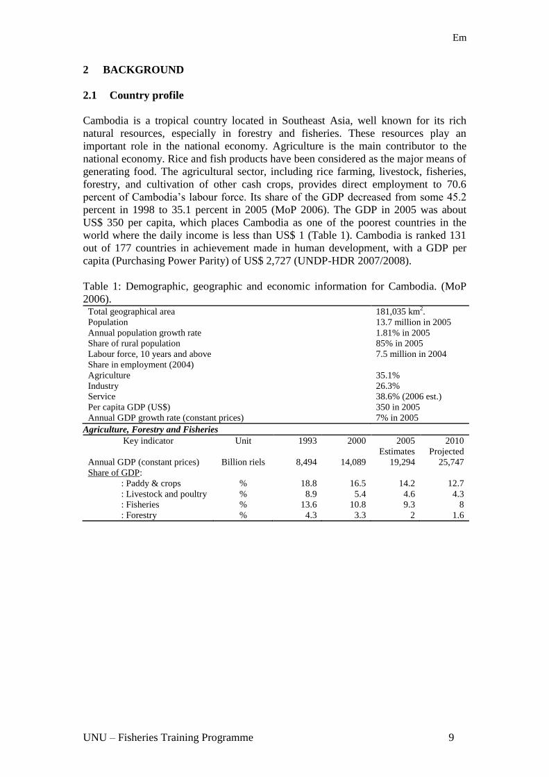
Em
UNU ndash Fisheries Training Programme 9
2 BACKGROUND
21 Country profile
Cambodia is a tropical country located in Southeast Asia well known for its rich
natural resources especially in forestry and fisheries These resources play an
important role in the national economy Agriculture is the main contributor to the
national economy Rice and fish products have been considered as the major means of
generating food The agricultural sector including rice farming livestock fisheries
forestry and cultivation of other cash crops provides direct employment to 706
percent of Cambodia‟s labour force Its share of the GDP decreased from some 452
percent in 1998 to 351 percent in 2005 (MoP 2006) The GDP in 2005 was about
US$ 350 per capita which places Cambodia as one of the poorest countries in the
world where the daily income is less than US$ 1 (Table 1) Cambodia is ranked 131
out of 177 countries in achievement made in human development with a GDP per
capita (Purchasing Power Parity) of US$ 2727 (UNDP-HDR 20072008)
Table 1 Demographic geographic and economic information for Cambodia (MoP
2006) Total geographical area 181035 km
2
Population 137 million in 2005
Annual population growth rate 181 in 2005
Share of rural population 85 in 2005
Labour force 10 years and above 75 million in 2004
Share in employment (2004)
Agriculture 351
Industry 263
Service 386 (2006 est)
Per capita GDP (US$) 350 in 2005
Annual GDP growth rate (constant prices) 7 in 2005
Agriculture Forestry and Fisheries
Key indicator Unit 1993 2000 2005
Estimates
2010
Projected
Annual GDP (constant prices) Billion riels 8494 14089 19294 25747
Share of GDP
Paddy amp crops
188
165
142
127
Livestock and poultry 89 54 46 43
Fisheries 136 108 93 8
Forestry 43 33 2 16
Em
UNU ndash Fisheries Training Programme 10
Figure 1 Map of Cambodia
22 Overview of the Cambodian marine fisheries sector
The marine fish stocks are a heavily exploited resource due to the high density of the
coastal population around the Gulf of Thailand Cambodia has a marine coastline of
435 km which covers two cities and two provinces The Exclusive Economic Zone
(EEZ) covers approximately 55600 km2 and is relatively shallow with an average
depth of about 50 m The marine fishing grounds are located on the eastern bank of
the Gulf of Thailand There are 525 species of marine finfish 20 species of marine
crabs 42 species of marine gastropods 24 species of marine bivalves and 11 species
of marine mammals (Tana 1997 Try 2003) Marine fisheries development has been
slow compared to the inland fisheries which are yielding approximately 400000
tonnes of fish annually The landed catch of marine fisheries was estimated at around
60000 tonnes in 2006 (FiA 2007)
Figure 2 Map of the coastal areas of Cambodia
Em
UNU ndash Fisheries Training Programme 11
221 Marine catches
The Department of Fisheries statistics (2004) cited by the Community Fishery
Development Office (CFDO 2005) reports that the annual marine catches were
estimated at about 36000 tonnes in 1994 ndash 2000 This number excludes the catches of
subsistence and illegal foreign fishing The Fisheries Administration has estimated the
increase in fish production from 36000 tonnes in 2000 to 60500 tonnes in 2006
(Table 2) which includes catch in mangrove areas due to the fact that the harvest of
mangroves is covered by the present fisheries law
In fact the actual catch of marine fisheries is higher than the official statistics suggest
This is because the catches from subsistence fishing including family-scale fisheries
are largely unrecorded Furthermore catches from illegal fishing activities are not
recorded Csavas et al (1994) state that information on the landing of marine fish in
Cambodia can be inferred from records of fish landings from the Thai portion of the
Gulf of Thailand This is partly due to the Thai vessels fishing in Cambodian waters
and some Cambodian fishing boats selling or transferring their catch to Thai mother-
vessels at sea or landing in Thai ports According to the DoF internal reports catches
from licensed Thai vessels in Cambodian water are estimated to be from 26500
tonnes to 37500 tonnes (Gillett 2004) Robert (Gillett R 2004) also concluded that if
this is indeed the case this amount would approach the total marine catch recorded for
all Cambodian fishing vessels operating offshore Substantial Thai catches in
Cambodian waters complicate any management strategy for Cambodian fish resources
because of difficulties associated with ensuring that rents from improved Cambodian
management actually benefit Cambodian fishermen and not only the less regulated
Thai fishing fleet
The marine fishery involves coastal fishers in inshore areas and foreign fishers
operating legally and illegally in offshore areas (NACA 2004) Cambodia currently
does not have the capacity to exploit offshore areas Since 1992 marine fisheries
statistics have included estimates of catches by foreign fishers licensed to operate in
the EEZ of Cambodia (DoF 2001d)
Table 2 Total fishery production inland and marine fishery from 2000-2006 (FiA
2007)
Year Total
(tonnes)
Inland (ton) Marine
(tonnes) Total Commercial
fisheries
Familysubsist
ence fisheries
Rice field
fisheries
2000 281600 245600 85600 110000 50000 36000
2001 427000 385000 135000 140000 110000 42000
2002 406150 360300 110300 140000 110000 45850
2003 363500 308750 94750 120000 94000 54750
2004 305800 250000 68100 106400 75500 55800
2005 384000 324000 94500 137700 91800 60000
2006 482500 422000 139000 181000 102000 60500
222 Catch by species and finfish production
Finfish is the main group of annual total catches by year (Table 3) Try (2003)
indicated that 33 species of finfish are commonly exploited Only five species are
very abundant in the landings Megalaspis cordyla (torpedo scad) Scomberomorus
commersoni (narrowbarred Spanish mackerel) Rastrelliger brachysoma (short
Em
UNU ndash Fisheries Training Programme 12
mackerel) Rastrelliger kanagurta (Indian mackerel) and Atule mate (yellowtail scad)
The volume of finfish caught in 2006 decreased slightly compared to 2005 but the
total catches have increased in 2006 as Anadromous fish (3678 tonnes) were not
record in 2005
The catches of trash fish each year rank the second after finfish (Table 3) In 1960 the
trawl gear was introduced to fishers in Cambodia that allows for catch of demersal
fish and juveniles During the past three decades trash fish was discarded due to no
demand and no value in the market But after 1993 a factory was built in Sihanoukvill
for processing trash fish for fish feed Therefore fishers catch and collect the trash
fish resulting in that the volume of trash fish has recently increased
As the market price of economic fishes has gradually been increasing trash fish have
become food for local people and particularly the poor coastal dwellers who have a
low income According to Try (2006) it was estimated that the trash fish caught by
trawl in 1980 is about 30-40 of the total catch but the percentage of trash fish was
recently increased probably to 60-65 of marine fish catches by trawl It seems that
to be encouraging the fishers use a more efficient gear to fish in inshore waters than
offshore Perhaps they are also using illegal fishing gears such as trawlers mosquito
net push and small mesh sizes of nets catching all fish species and sizes The marine
fish catches in 2006 have declined for all groups except shrimp from 2005 (Table 3)
Table 3 Statistics of marine fisheries caught by groups in Cambodian coastal waters
(in tonnes) (Try et al 2006 and FiA 2007)
Yea
r
Fin
fish
Tra
sh f
ish
Sh
rim
p
pra
wn
s
Ray
s
Sq
uid
cutt
lefi
sh
Lo
bst
ers
Cra
bs
Gas
tro
po
ds
Sea
slu
g
An
adro
mo
us
fish
To
tal
mar
ine
fish
ery
2000 15526 9833 2905 245 2627 59 3593 801 11 410 36010
2001 16873 10847 3872 209 2355 40 3462 3681 0 661 42000
2002 18910 11752 3827 553 2681 122 3545 3007 3 1410 45810
2003 26596 14859 4055 727 3577 169 4028 648 2 61 54722
2004 25639 16570 3824 620 2984 124 3458 2457 0 124 55800
2005 26141 18265 4124 996 3723 1233 4301 1215 2 0 60000
2006 25641 17194 4778 476 3551 115 4180 897 0 3678 60500
Almost 90 of the marine fisheries production in Cambodia is from two coastal
provinces Sihanoukvill and Koh Kong (Table 4) The total catches of finfish are
mackerel fish amount 4650 tonnes (FiA 2007) The trash fish is second in rank
among the group species caught of which Koh Kong and Sihanoukvill rank at the top
Table 4 Statistics of marine product of four main coastal areas 2006 (FiA 2007)
Cit
y
pro
vin
ce
Fin
fish
Tra
sh f
ish
Sh
rim
p
pra
wn
s
Ray
s
Sq
uid
cutt
lefi
sh
Lo
bst
ers
Cra
bs
Gas
tro
po
ds
An
adro
mo
us
fish
To
tal
mar
ine
fish
erie
s
Kampot 2103 1674 386 32 130 5 635 415 2000 7380
Kep 300 - 35 5 10 - 45 17 18 430
Koh Kong 13519 10500 1622 89 1100 - 2000 280 160 29270
Sihanoukvill 9709 5020 2735 350 2311 110 1500 185 1500 23420
Total 25631 17194 4778 476 3551 115 4180 897 3678 60500
Em
UNU ndash Fisheries Training Programme 13
223 Costal fishers and employment
Most coastal fishers are poor and generally use small-scale fishing gear that is only
adequate for use inshore and in mangroves There are limited numbers of coastal
fishers that have sufficient capital to invest in the necessary vessels and gear for
offshore fishing The capacity of fishers fishing offshore in the EEZ is not large
compared to the potential exploitation
Officially the statistics of fisheries employment have shown only the number of
people involved in fisheries harvesting processing and culturing There are no
statistics on other numbers of people employed in fisheries related activities The
number of fishers and the number of fish processor is reflected in Table 5 below
Table 5 Statistics of fishers and processors 1999-2006 (DoF‟s Statistics 2000-2006) Year Harvesting labour force in marine sector
Processing labour
force Familyrice field
Mobileartisanal
Fisheries Total fishers
No of
families
No of
fishers
No of
families
No of
fishers
No of
families
No of
fishers
No of
families
No of
processors
1999 0 0 3910 11721 3910 11721 373 1527
2000 0 0 6557 14647 6557 14647 379 1631
2001 6445 8067 4137 15350 10582 23417 370 1499
2002 24818 45940 9648 26130 34466 72070 1472 2379
2003 16047 28638 13159 40014 29206 68652 990 1815
2004 16475 31657 10865 33274 27340 64931 1407 4234
2005 - - - - - - - -
2006 18949 37990 12006 36582 30955 74572 1226 29412
224 Number of vessels
Non-motorised and motorised vessels are used in Cambodia‟s marine fisheries Most
non-motorised vessels are used by the small-scale fishers who carry out subsistence
fishing The Fisheries Department has statistically categorised the non-motorised
vessels based on their dead weight The three categories are less than 5 tonnes more
than 5 tonnes and Duk-boats but the Duk-boat is not directly used for fishing (ie it
is used for transporting the fisheries products)
The motorised vessels are divided into four categories based on engine power less
than 10 hp 10 to 30 hp 30 to 50 hp and more than 50 hp This classification does not
include data on the number of vessels involved in small-scale and large-scale
fisheries
The number of non-motorised vessel in 2000 was only 255 and increased to 841 boats
in 2002 operating within Cambodia‟s coastal zone then it dropped dramatically to
272 boats in 2004 and increased again to 821 boats in 2005 and 1059 boats in 2006 as
illustrated in Figure 3
Noticeably the number of motorised fishing vessels seems to increase linearly from
5037 boats in 2000 to 7027 boats in 2005 and drop to 6236 boats in 2006 Most of
the motorised fishing vessels with large fishing gears are required to have licenses to
operate Two systems exist of motorised fishing vessels licenses one is a license
issued by the provincial fisheries office for all motorised vessels equipped with engine
Em
UNU ndash Fisheries Training Programme 14
power under 33 horse power (hp) and another is a license issued by the Fisheries
Administration for all motorised vessels equipped with an engine power above 33
horse power (hp)
Referring to regulations on offshore and inshore vessels it can be assumed that all the
motorised vessels which have small engine power (below 50 hp) and non-motorised
vessels operate inshore Motorised vessels equipped with engine power greater than
50 hp should operate offshore
Fishing vessels equipped with engine power higher than 50 hp may use a labour force
from 5 to 15 people depending on the fishing gear used For boats with an engine
power higher than 100 hp the labour force may be 15 to 30
Figure 3 Number of marine fishing vessel from 2000-2006 (FiA 2007)
225 Annual contribution of marine fisheries to the economy
According to a government report the marine capture fishery has increased from
36000 tonnes in 2000 to 60500 tonnes in 2006 (Table 2) Thus the average marine
capture fishery was around of 50700 tonnes per year from 2000 to 2006 Try et al
(2006) mentioned that the average market price of marine fish is US$ 1 per kg The
marine capture fishery can be estimated to value US$ 507 million a year at the
market site If the tourism industry in Cambodia shows a steady increase of 20
yearly (MoT 2007) the demand for food consumption for tourists will increase This
leads to an increase in the domestic market price of marine fish in Cambodia and the
marine capture fisheries in 2006 can be estimated to value in total revenue around
US$ 635 million According to Try et al (2006) the capture marine fishery values
account of US$ 15 million to US$ 30 million excluding the illegal export which is
un-reported This estimation was at the average market price of trashfish at 500
Cambodian Riels per kg The share of fisheries in the GDP or government revenue
was 108 in 2000 and the estimate for 2005 is 930 (Table 1)
226 Fisheries landing ports
Landing locations are not separated from fishing locations and harbour facilities are
limited Much of the catch is transferred to Thai vessels at sea for landing in Thailand
(FAO 2005) Landing sites of four main coastal areas are used for statistics a total of
about 131 locations landings exist in Sihanoukvill 69 Koh Kong 55 Kampot 4 and
Em
UNU ndash Fisheries Training Programme 15
Kep City 3 Most landing ports are small and rural services and facilities are poor It
may be concluded that fishery landing ports of four main coastal provinces are not of
interest to the private sector to invest in rather these are subsidised by the
government
23 Mackerel fisheries
Mackerel consists of commercial pelagic groups which include short mackerel Indian
mackerel Indo-Pacific mackerel Spanish mackerel and island mackerel They are the
most important pelagic species in the Gulf of Thailand harvested by commercial and
traditional gears The local name ldquoPlathu Kamongrdquo is used loosely to refer to all
these fish species
231 Mackerel production
The highest recorded annual landing of mackerel (Rastrelliger) was 139220 tonnes
and contributing 14 to all the marine fish landed in 1968 in the whole Gulf of
Thailand Second to this 122156 tonnes or 11 of the marine fisheries landings were
recorded in 1969 (Sea Around Us 2005) These species supported the purse seine and
gillnet fisheries since the early 1960s and have remained important until now In fact
mackerel is the most dominant commercial food fish in the Gulf of Thailand
The catch of mackerel declined from about 40000 tonnes in the 1950s to around 20000
tonnes in the 1980s An unusually sharp increase in catch occurred though in 1965-1971
when the catch reached 140000 tonnes The pressure from the industry in Thailand has
resulted in overexploitation Ahmed et al (2007) state that ldquofor a number of decades
fisheries development in the Gulf of Thailand has concentrated on increasing fishing
effort to maintain or increase the production volumerdquo Most important pelagic fish in
the Gulf of Thailand are fully exploited especially Indo-Pacific mackerel anchovies
round scad and sardines and demersal resource stocks are over-fished (FAO 1995)
Figure 4 Volume of mackerel caught in the Gulf of Thailand from 1950-2004 (Sea
Around Us 2005)
232 Mackerel fisheries exploitation and its catch effort in Cambodia
Mackerel is not only sold on the domestic market but is also exported to Thailand
every year both fresh and processed Mackerel in Cambodia is caught by artisanal
fishermen as well as the industrial fishery The artisanal fishery operates from small
Em
UNU ndash Fisheries Training Programme 16
boats with outboard engines of less than 33 hp Most of these fishing boats use
gillnets to catch in inshore areas The industrial mackerel fishery is operates offshore
using purse seines or driftnets with boat engines up to 50 hp The commercial fishing
boat can stay at sea fishing 2 to 5 days This type of boat has facilities to keep fish for
long time
Since 1990 the catch of mackerel by Cambodia had increased from about 1000
tonnes to 4650 tonnes in 2006 (Table 6) From 2002 to the present the catch has been
stable at around 4500 tonnes but the effort has increased with a corresponding
reduction in CPUE
The gillnet boats fish for mackerel approximately 25 days a month 8 months a year
The purse seine operates only during the dry season period of 5 months (20 days per
month) The purse seine boats have crews of about of 15 to 30 people The gillnet
boats can on the other hand operate with a labour force of only 2 to 3 people
Table 6 Volume caught fishing effort and CPUE of mackerel from 1990-2006 (FiA
2007)
Year
Catches
volume
(tonnes)
Fishing effort CPUE
(Kgperson
day)
Boat used gillnet Boat used purse seine Total
boat
Total
labour Boat Labour
(person) Boat
Labour
(person)
1990 1395 - - - - - - -
1991 1212 - - - - - - -
1992 1101 3 9 13 260 16 269 40
1993 1424 9 27 14 280 23 307 43
1994 1513 31 93 15 300 46 393 31
1995 1683 10 30 16 320 26 350 44
1996 1452 14 42 6 320 30 362 36
1997 1278 114 342 15 300 129 642 13
1998 1447 122 366 15 300 137 666 14
1999 1738 172 516 8 160 180 676 15
2000 1559 155 465 10 200 165 665 14
2001 1731 56 168 10 200 66 368 32
2002 4300 50 150 10 200 60 350 86
2003 4421 73 219 13 260 86 479 63
2004 4764 117 351 10 200 127 551 53
2005 4906 250 750 4 80 254 830 31
2006 4650 181 543 6 120 187 663 39
233 Mackerel fish processing products
The mackerel in Cambodia is traditionally processes by salted or steaming For
steamed fish ldquoshort body mackerelrdquo is the local name called as Trey Chom Houy but
for salting ldquoSpanish mackerelrdquo is used the local name is Trey Borb Most production
is for the domestic market Data is limited on export
234 Marketing and price of mackerels
Locally the price of mackerel and its products can be different between markets
throughout the land However the difference between the markets of the four
Cambodian coastal areas is small The Sihanoukville market site is the main
Em
UNU ndash Fisheries Training Programme 17
distribution centre of marine fisheries products into the local market thus the market
price of Mackerel fishes and its products in Sihanoukvill can be assumed as the local
market standard price of Mackerel fishes and its products According to monthly
reports of the Marine Fishery Division the price of mackerel at the landing site and
domestic market is actually increasing especially in the wet season when catch is
small and but demand is high
In 2006 the price of short mackerel at the landing site from January to September
fluctuated from US$ 450 to US$ 625 per tonne1 (Figure 5) Based on data estimated
by the Fishery Administration the landing volume of mackerel species in 2006 was
about 4650 tonnes and can be estimated at around US$ 252 million or 4 of the
marine fishery revenue in 2006 Spanish mackerel is selling at a high price at the
landing and market site but the landing volume is small compared to short mackerel
The landing price of Spanish mackerel within a 9 month period in the year 2006
fluctuated increasingly from US$ 1375 to US$ 3500 per tonne Figure 5 illustrates
the price of short mackerel and Spanish mackerel correlated at two sites domestic
market and local landing site
In general the price of marine fish at landing as well as market site has increased over
the years due to an increase in the fishing operational cost Moreover increased
population leads to high market demand for human consumption whereas the natural
resources are gradually decreasing Thuok et al (2001) stated that marketing channels for
marine products are not so well developed for food security and economy reasons it is
believed that emphasis should be placed by the administration in support of the private sector
on the development and enhancement of marketing of marine fishery products
Figure 5 Price of mackerels at landing and market site for 9 months in 2006 (FiA
2007)
1 The price of mackerel at landing site was conducted and reported to the Fishery Administration by Marine
Fishery Division from January to September in 2006
Em
UNU ndash Fisheries Training Programme 18
24 Marine fisheries resources management in Cambodia
241 Law and regulation
The Cambodian marine fishery is managed under the Fisheries Law of 2006 which is
an improved and updated version of the law from 1987 The main objective of the law
and regulation is to manage and conserve the marine fishery resources in a sustainable
manner Additional objectives are to generate governmental revenue improve the
livelihood of local communities and achieve ecologically sound management by an
improved statistical system gear restrictions area limitations and time closures
Management objectives other than those in the Fishery Law 2006 exist and are
attained by the Ministry of Agriculture Forestry and Fishery (proclaim issue) ie
closed season from 15 January to 31 March for mackerel species
For management purposes the marine fisheries are divided into two groups
Coastal fisheries small family-scale fishing operating in fishing zone 1 which
extends from the coast to a depth of 20 m this fishing zone was almost managed by
community fisheries The coastal community fisheries were established after the
government recognised the poor management of the fisheries sector which resulted in
a movement for reform in 2000 Nowadays 40 community fisheries have been
established along the coast to encourage coastal dwellers to participate in the
management of their resources Fishers use boats without engines or with engines of
less than 50 hp Licenses are not required for boats with no engine or with engines
below 33 hp but for boats with more than 33 hp engines a license fee of 27000 Riels
(US$ 7) per horsepower per year is required Fishing activities are not allowed to
include other fishing gears such as trawls or light fishing
Commercial fisheries refer to large-scale fishing from 20 m depths to the limits of the
EEZ Boats used have engines with more than 50 hp which must be licensed for a fee
of 27000 Riels (US$ 7) per horsepower per year Prohibited fishing gears and
methods include pair trawling light fishing and other illegal fishing gears All marine
fisheries are open year round apart from mackerel for which fishing is banned from
15 January to 31 March (DoF 2001d) Most of the small boats (engine lt 50 hp)
marine fishing fleets use alternative multi-fishing practices following the seasonal
appearance of marine resources including purse-seines gill nets push nets and
trawling Foreign poachers use prohibited gears such as large bottom trawls long drift
nets pair trawlers light fishing and explosives (DoF 2001d)
242 Management and administration
Despite a few limitations on the fisheries in the Gulf of Thailand fisheries there fall
under the framework of unregulated open access In addition there are no limits
placed on the amount of gears that can be used the amount of time that can be spent
fishing or on the quantity of fish that may be captured
Generally coastal fishers can operate all year round by using many different types of
fishing gears However the use of fishing gears is dependent on a number of critical
factors including (1) the capital invested (2) experience and traditions of the fishing
communities in different locations along the coast (3) seasonal abundance of different
Em
UNU ndash Fisheries Training Programme 19
species (4) seasonal weather conditions and (5) ecological conditions associated with
the fishing grounds (eg inshore offshore mangrove coral reef etc)
Fishing in offshore areas is still a challenge and there is a lack of strong law
enforcement measures against illegal fishing from neighbouring countries It is a
problem represented in the low annual production of marine fisheries The present
management of data collection is not sufficient to develop plans for scientific
management of marine fish stocks The lack of knowledge of fish biology ecology
and their dynamics results in a poor understanding of the recent changes in marine
fish stocks (MAFF-DoF 2004)
On the other hand the fisheries competency is still inadequate This is true in terms of
inspection specialists and the lack of adequate physical means to enforce legislation
such as protection against illegal fishing (ie the Fisheries Administration is less able
to set up or install the right technology a high speed boat radio communication and
other facilities for coast guard operations) Furthermore in the 1990s the political
environment was unstable which affected the business environment and led to less
investment capital
However the government and Fisheries Administration have overcome many
obstacles to develop and manage marine fisheries resources as well as the fisheries
sector in the past years Especially a recent achievement is the Fishery Law
completely promulgated public using in 2006 (FiA 2007) The new law was updated
from the previous Fishery Law of 1987 which was based on legislation from 1956
1958 and 1960 (revised) The updated law was also drafted with participation from
stakeholders IOs NGOs and relevant partners through research study and sustainable
development projects on the fisheries sector framework In terms of gains marine
production through fishing effort as well as improve capacity of fishing and biomass
management in EEZ
3 THE PRINCIPLES OF FISHERIES MANAGEMENT
This chapter has been adapted from the lecture notes in the UNU-FTP specialist
course on Fisheries Policy and Planning by Prof Ragnar Arnanon
The need for fisheries management stems fundamentally from the fact that fish
resources are common property It is well known both from theory and experience
that common property resources will be overexploited and possibly irreversibly
depleted unless subjected to appropriate fisheries management Essentially the
fisheries management regime is a set of social prescriptions and procedures that
control the fishing activity Similarly fisheries management requires either collective
action at the industry level or external usually government intervention
The principles of fisheries management or fisheries management regimes consist of i)
the fisheries management system (FMS) ii) monitoring control and surveillance
(MCS) and iii) fisheries judicial system (FJS) These three components of the
fisheries management regime are strongly interdependent All three components of the
fisheries management regime are crucial to its success They are links in the same
chain If one of them fails the fisheries management regime as a whole fails
Em
UNU ndash Fisheries Training Programme 20
31 The fisheries management system (FMS)
The fisheries management system specifies the regulatory framework for the fishing
activity It consists of all the rules that the fishing activity must obey such as gear and
area restrictions fishing licences catch quotas etc In many countries most fisheries
rules are based on explicit legislation In others they are primarily based on social
customs and conventions
The fisheries management system is basically a set of rules about how the fishery
should be conducted These rules may be formal ndash for instance in the form of
published laws and regulations ndash or they may be informal ndash a part of the social culture
governing fishing behaviour In most fisheries both types of fisheries management
rules the formal and the informal apply The purpose of the fisheries management
system is to contribute to the generation of net economic benefits flowing from the
fishery
The fisheries management represents the application of specific fisheries management
instruments or tools Typical fisheries management tools are for instance fishing gear
restrictions limitations on the number of allowable fishing days during the year area
closures and so on Thus the fisheries management tools are like variables or more
precisely control variables and the fisheries management measures the values that can
be chosen for these control variables
Now fisheries management systems consist of particular combinations of one or more
of these tools Thus obviously the number of possible fisheries management systems
increases very fast with the number of available fisheries management systems Most
of them may however be grouped into two broad classes i) Direct fisheries
management and ii) indirect fisheries management as illustrated in Figure 6
Figure 6 Fisheries management systems a classification (adapted from lecture notes
UNU-FTP 2007 introduced by professor Arnason)
Direct fisheries management attempts to control the components of the fishing
activity directly by commands or more often restrictions that must be adhered to
Indirect economic fisheries management by contrast attempts to induce the fishing
firms to behave differently by modifying the operating conditions of the fishery
without imposing direct constraints The difference between direct biological and
economic fisheries management lies in what they seek to control Direct biological
fisheries management attempts to alter the biological yield of the fishery Thus under
biological fisheries management for instance the sustainable yield curve is normally
shifted Direct economic fisheries management attempts to alter the behaviour of the
Em
UNU ndash Fisheries Training Programme 21
fishing firm days vessel size etc Thus direct economic management generally
affects the cost structure of the fishery directly
Indirect fisheries management alters the operating conditions of the fishing industry
There are of course many ways to do this Most however belong to two main
categories (a) taxes (and subsidies) which basically alter the prices facing the fishing
industry and (b) property rights which alter the nature of the external effects imposed
by the fishing firm on one another
Most fisheries management tools are fall quite naturally into one of the fisheries
management categories in Figure 6 The main exception is the total harvesting
restriction or total allowable catch (TAC) Of all the fisheries management systems
considered above only (i) certain property right arrangements and (ii) tax on catch
seem to be theoretically capable of delivering the full potential economic benefits of
fisheries Direct fisheries management irrespective of whether it is based on
biological or economic restrictions seems particularly inept for this purpose
Em
UNU ndash Fisheries Training Programme 22
32 Monitoring control and surveillance (MCS)
The primary task of the monitoring control and surveillance system is to observe the
fishing industry‟s activities and to enforce its adherence to the rules of the fisheries
management system Its secondary but nevertheless very important task is to collect
data about the fishery that can be used to improve both the fisheries management and
fisheries judicial system as well as the monitoring control and surveillance system
itself Broadly speaking the phrase refers to two activities i) the monitoring of the
fishery and the activities of the fishing (harvesting) industry and ii) the enforcement
of fisheries management rules
MCS is as already discussed a crucial component of any fisheries management
regime Logically it is the management authority that must conduct and co-ordinate
the MCS activity although it may engage contractors it is the central fisheries
manager ie the government that operates the MCS activity
The monitoring part of MCS involves collection of the relevant biological data about
the fish stocks and the surrounding ecosystem as well as the relevant technical
economic and behavioural data about the fishing industry and its activities The
monitoring activity is conducted for essentially two purposes i) to gather information
for improving the fisheries management ie data generation monitoring and ii) to
gather information for the purpose of enforcing existing fisheries management rules
ie enforcement monitoring It is important to realise that in order to transform
fisheries data into sensible decisions on fisheries management measures and
modifications of the fisheries management system a good deal of biological and
economic research has to take place Hence is should be clear that research both
biological and economic is an integral part of the monitoring part of the MCS
activity
The enforcement part of MCS consists of acting upon alleged violations of fisheries
management rules It generally takes place where and when the violating activity
occurs The action taken may be of several degrees of severity i) induce the violator
end the illegal activity ii) impose a penalty ie an administrative penalty typically a
fine or a temporary revoking of fishing licence iii) indict the alleged violator and iv)
apprehend and indict the alleged violator In this case the alleged violator is
apprehended (a penalty in itself) and also formally charged for the offence
It should be clear that if the fishing firms are profit maximisers enforcement action
will in general not suffice to generate sufficient adherence to the fisheries
management rules unless the level of monitoring and enforcement is extremely
highly relative to the fishing activity Since the former implies that a decentralised
fishery can never be efficient and the latter is obviously far too expensive compared to
the value of the fishery we may conclude that any reasonable MCS system must rely
on (ii)-(iv) to a significant extent For later reference it is useful to note that the
enforcement part of MCS especially degrees (iii) and (iv) above is linked to the
operations of the fisheries judicial system and in fact depends on it if it is to be
effective
The cost of MCS in fisheries is by no means negligible The available indications
(Arnason et al 2002) suggest that this cost usually ranges between 2 and 10 of
Em
UNU ndash Fisheries Training Programme 23
the total landed value of national the fisheries According to Arnason et al (2002) the
most important MCS cost items appear to be i) enforcement at sea and on land ii)
data collection and research and iii) policy formulation and system administration
Enforcement costs especially those at sea are generally very high and as a whole
usually account for well over half of the total MCS costs Data collection and research
costs typically account for over a third of the total MCS costs with the most costly
item being biological research The rest of MCS costs are accounted for by policy
formulation and general administration costs
33 Fisheries judicial system (FJS)
The fisheries judicial system is part of the general judicial system It should be noted
however that in most societies the formal judicial system is to process alleged
violations of fisheries management rules and issue sanctions to those deemed to have
violated the rules The fisheries judicial system thus complements the monitoring
control and surveillance activities in enforcing the fisheries management rules
The purpose of the fisheries judicial system (FJS) is to i) process alleged violations of
fisheries rules and ii) apply sanctions as appropriate It follows that the FJS must
contain well defined procedures as to how to process alleged violations What are the
courts how may cases be referred to the courts what are the appeal procedures time
limits and so on Without the support of the fisheries judicial system the MCS
activity would not work Alleged violators would simply go to court and get off with
penalties insufficient to deter them from their illegal activities Hence the MCS
activity would be of little use In particular it would not succeed in enforcing the
fisheries rules
It is often found that the fisheries judicial system is the weakest link in the fisheries
management regime The public information and awareness of the judicial system is
not well distributed and the people then are not well-informed Fundamentally the
judiciary system is fairly independent of the executive and legislative branches of
government As a result the fisheries management regime is much less amenable to
reform and change than the other two components The trials and judgements are
passed according to law custom and convention The judicial system in executing
laws and judgements generally has little understanding of the intricacies of the FMR
This suggests the need to include carefully designed laws concerning the treatment of
fisheries violations the burden of proof penalties etc in the fisheries legislation
defining the fisheries management regime
The main objective of the FJS is to endorse the enforcement part of the MCS activity
In particular the FJS determines crucial components of the probability that a violator
of fisheries legislation will suffer penalties The adherence to fisheries management
rules requires sufficiently high administrative costs in processing these allegations
Generally any expected cost of violations can be generated by the appropriate
combination of enforcement and penalties To find this appropriate combination it is
necessary to obtain an empirical estimation from the increased enforcement activity
and improved FJS and its implications to the expected costs of violations
Em
UNU ndash Fisheries Training Programme 24
4 MODELLING
The bio-economic model applied in this chapter has been adapted from the lecture
notes in the UNU-FTP specialist course on Fisheries Policy and Planning by Prof
Ragnar Arnanon
The model applied in this report is used to explain the mackerel fishery in Cambodia
and investigate improvements in its utilisation it is a simple bio-economic model of
the fishery resources The model chosen is based on the work of Gordon (1954) and
Schaefer (1957) (Anderson G L 1981) who developed a basic bio-economic model
for fisheries management The main elements of this model are i) a biomass growth
function which represents the biology of the model ii) a harvest function which
constitutes the link between the biological and economic part of the model and iii) a
fisheries profit function which represents the economic part Particularly for
prediction of the maximum sustainable yield (MSY) of the mackerel fishery we apply
the ldquosurplus production modelsrdquo a simple model introduced by Graham (1935)
(Anderson G L 1981) but they are often referred to as ldquoSchaefer modelsrdquo This
approach was selected for the following reasons i) the Cambodian mackerel fishery
data is very limited and thus does not support an advanced bio-economic model ii)
the model developed here can later be extended and refined when more and better
data becomes available More precisely the model is as follow
x = G(x) ndash y (Biomass growth function) (1)
where x represents biomass x is biomass growth and y is harvest The function G(x) is
natural biomass growth
y = Y(ex) (Harvesting function) (2)
The volume of harvest is taken to depend positively on fishing effort as well as the
size of the biomass to which the fishing is applied
π = p∙Y(ex) ndash C(e) (Profit function) (3)
Where p represents the price of fish landing and C(e) is the cost function of fishing
effort The profit function depends on the fish price the sustainable fish yield and the
fishing operation costs The fishing costs depend on the use of economic inputs
which is the fishing effort can represent the profit function equation
The above model comprises three elementary functions the natural growth function
G(x) the harvesting function Y(ex) and the cost function C(e) It adopts the widely
used specific form for these functions
41 The biomass growth function
Populations of organisms cannot grow infinitely the growth of organisms is
constrained by environmental conditions and food availability It has been shown that
populations of organisms strive to stabilise at the highest possible population size for
a given set of conditions (Schaefer 1954) (Anderson G L 1981) Marginal growth of
a population increases when the size of the population decreases and marginal growth
Em
UNU ndash Fisheries Training Programme 25
decreases when the size of the population increases this may be called density
dependent growth Biological growth of such populations may be expressed as
follows
G(x) = rx ndash sx2 (4)
Where x is population size r is the growth rate of the population and s is the mortality
rate which is negative This is the parabolic equation also referred to as Verhults‟
equation or the logistic growth equation (Schaefer 1954) (Anderson G L 1981)
When the population reaches the environmental carrying capacity (K) growth and
mortality of the population is equal and rate of change of population size with respect
to time (dxdt) becomes zero The mortality rate s can now be expressed in terms of r
and K as
(5)
From equation (5) substitute s in equation (4) we get the most commonly used
expression of the logistic growth equation and equation (4) can be rewriten as
(6)
Fox (1970) (Arnason R 2007) outlined an alternative surplus yield model assuming
the Gompertz growth function resulting in an exponential relationship between
fishing effort and population size and an asymmetrical harvest curve (Fox 1970)
(Arnason R 2007) The generalised form of the Gompertz curve can be represented
as (Winsor 1932) (Arnason R and Bjorndal T 1991)
F(x) = micro∙x(lnK ndash lnx) (7)
In this formulation the carrying capacity of the biomass is K as in the logistic
formulation However unlike the logistic the Fox-Gompertz growth function is not
symmetric and the intrinsic growth rate is infinite compared to r for the
logistic
The major difference between the logistic model and the Fox model is that at lower
population sizes the Fox model predicts a higher growth rate than the logistic model
At higher population sizes the logistic model predicts a higher growth rate than the
prediction by the Fox model In the logistic model maximum growth occurs at half of
the maximum population level In the Fox model maximum growth occurs at a
population level of less than the half of the maximum population around 37 of the
maximum population On the other hand the population growth curve of the Fox
model is skewed to the left while the population growth curve of logistic model is
symmetrical
Em
UNU ndash Fisheries Training Programme 26
Figure 7 Illustrates the logistic biomass growth model G(x)
Figure 8 Illustrates the Fox biomass growth model G(x)
For biomass growth we consider the logistic and the Fox
G(x) = α∙x - β∙x2
(8)
F(x) = α∙x - β∙ln(x)∙x (9)
42 The harvesting function
Assuming that each unit of effort harvest equals the amount from the targeted stock
and an equilibrium situation where catch equals natural growth the equilibrium stock
size (x) may be expressed in terms of carrying capacity (K) catchability coefficient
(q) and fishing effort (e) For the harvesting model in accordance to the generalised
Schaefer (1954) (Anderson G L 1981) version
Y(ex) = q∙e∙xb (10)
Where the coefficient b indicates the degree of schooling behaviour by the fish which
b Є[01]
43 The cost function
Consequently the costs of fishing effort will be a linear function of the amount of
effort ndash index of economic input in the form of labour investment fuel maintenance
and supplies fixed costs and overhead that is devoted to the fishery on an annual
basis The annual cost of fishing C(e) is proportional to effort (e) For this report it
was assumed that the fishing boats are homogeneous The cost function is expressed
as
Em
UNU ndash Fisheries Training Programme 27
C(e) = c∙e + fk (11)
Where c represents marginal costs and fk represents fixed costs
44 The complete model
The complete model based under those function specifications becomes
Biomass growth function
- = α∙x - β∙x2 ndash y (Logistic) (12)
- = α∙x - β∙ln(x)∙x ndash y (Fox 1970) (13)
Harvesting function
- y = q∙e∙xb (14)
Profit function
- π = p∙y ndash c∙e + fk (15)
The last two equations can be combined to yield a simpler version of the model
- π = p∙y ndash(cq)∙y∙x-b
+ fk (16)
The ratio (cq) is viewed as a single parameter known as the normalised marginal cost
It is shown that the marginal cost and catchability c and q are not displayed in an
independent role in this model What counts in the model is the ratio of the two
constant parameters
45 Sustainable yield
The annual rate of renewal of fish stock depends on three major factors biological
environment physical environment and magnitude of the remaining population
Biological and physical environment may be considered to be constant in the long run
(Schaefer 1954) (Anderson G L 1981) Population size is reduced by natural and
fishing mortality Harvesting increases the total mortality As the fish population
strives to balance the total mortality with growth the population reaches a new
equilibrium at a point where the growth rate equals total mortality which occurs at a
lower population size than the environmental carrying capacity level K When the fish
stock reaches equilibrium with a given effort level all biological growth of the
population is harvested and there is no need for change in the population size
y(ex) = G(x) (17)
(18)
and when
Em
UNU ndash Fisheries Training Programme 28
(19)
by substituting x in the equation (18) with equation (19) we get the long term catch
equation
(20)
This implies that although harvest is a function of effort and stock size for the short
term in the long run stock size becomes only a function of effort (given that
environmental conditions are constant) and the sustainable yield too becomes a
function of effort only
Equation (8) takes the form of a parabolic equation which allows us to use linear
regression in order to estimate the parameters of the function of sustainable harvest
(y) Dividing both sides of equation (8) by effort (e) we get the linear equation of
catch per unit effort (CPUE)
(21)
Assuming that biological growth of the subjected population follows the model
suggested by Gowpertz and also assuming the fleet is homogenous and all vessels
have the same fishing power
(22)
by substituting x in equation (6) with (22) the equation became as below
(23)
Dividing both sides of equation (23) by fishing effort (e) yields
(24)
A long-linear expression is found by
(25)
46 Maximum sustainable yield (MSY)
The objective of the application of the ldquosurplus production modelsrdquo is to determine
the optimum level of effort that is the effort that produces the maximum yield that can
be sustained without affecting the long-term productivity of the stock the so-called
maximum sustainable yield (MSY) Because holistic models are much simpler than
analytical models the data requirements are also less demanding There is for
example no need to determine cohorts and therefore no need for age determination
Em
UNU ndash Fisheries Training Programme 29
This is one of the main reasons for the relative popularity of surplus production
models in tropical fish stock assessment Surplus production models can be applied
when data are available on the yield (by species) and of the effort expended over a
certain number of years The fishing effort must have undergone substantial changes
over the period covered The basic models were expressed as follows
461 Surplus production models
The maximum sustainable yield (MSY) can be estimated from the following input
data
- f(i) = effort in year i where i = 1 2 3 hellip n
- Y(i) = yield in year i where i = 1 2 3 hellip n
- Yf = yield (catch in weight) per unit of effort in year t
Yf may be derived form the yield Y(i) of year i for the entire fishery and the
corresponding effort f(i) by
(i) Yf = Y(i) f(i) where i = 1 2 3 hellip n (26)
The simplest way of expressing yield per unit of effort Yf as a function of the effort
f is the linear model suggested by Schaefer (1954) (Anderson G L 1981)
(ii) Y(i) f(i) = a + b f(i) if f(i) le -ab (27)
The intercept ldquoardquo is the Yf value obtained just after the first boat fishes on the stock
for the first time The intercept therefore must be positive The slope ldquobrdquo must be
negative if the catch per unit of effort Yf decreases for increasing effort f Thus -ab
is positive and Yf is zero for ldquofrdquo = -ab (Sparre P and Venema C S 1998) The
equation (27) is a statistically estimable version of equation of equation (21) Schaefer
model
An alternative model was introduced by Fox (1970) (Arnason R 2007) It gives a
curved line when Yf is plotted directly on effort ldquofrdquo but a straight line when the
logarithms of Yf are plotted on effort
(iii) Ln(Y(i) f(i)) = c + d f(i) where ldquocrdquo is ldquoardquo and ldquodrdquo is ldquobrdquo (28)
Equation (28) is called the ldquoFox modelrdquo which can also be written
(iv) Y(i) f(i) = exp(c + d f(i)) (29)
Equation (29) is a statistically estimable version of equation (25) Fox model
Both models conform to the assumption that Yf declines as effort increases but they
differ in the sense that the Schaefer model implies one effort level for which Yf
equals zero namely when f = -ab whereas in the Fox model Yf is greater than zero
for all values of ldquofrdquo
Em
UNU ndash Fisheries Training Programme 30
However to obtain an estimate of the maximum sustainable yield (MSY) and to
determine at which level of effort MSY may be rewritten equations (27) and (29)
expressing the yield as a function of effort by multiplying both sides of the equation
by f(i)
Schaefer
(v) Y(t) = a f(i) + b f(i)2 if f(i) lt -ab (30)
Or Y(i) = 0 if f(i) = -ab
(vi) Y(i) = f(i) exp(c + d f(i)) (31)
From equation (30) the Schaefer model is a parabola which has its maximum value
of Y(i) the MSY level at an effort level
(vii) (32)
and the corresponding yield
(viii) (33)
From equation (31) the Fox model is an asymmetric curve with a maximum
sustainable yield level with a fairly steep slope on the left side and a much more
gradual decline on the right of the maximum The YMSY and fMSY for the Fox model
can be calculated by formulas which are derived from equation (31) by differentiating
Y with respect to ldquofrdquo and solve dYdf = 0 for ldquofrdquo
(ix) (34)
(x) (35)
The estimation procedures for the parameters (Schaefer a amp b Fox c amp d) will be
explained on the basis of the data given in Table 7 Since we are dealing with a
straight line in the case of the Schaefer model and a curve which has been linearised
by taking the logarithm in case of the Fox model the determination of a b and c d
requires two linear regressions of f(i) on Y(i)f(i) and f(i) on ln(Y(i)f(i)) respectively The
results of the two regressions are presented in Table 7 including a maximum
sustainable yield and its correspondent optimum level of effort Thus are determined
the relationships between catch per unit of effort and effort for both models
462 Biomass dynamic models
The formulation of the Schaefer surplus production model in its continuous and
discrete form the logistic model to include catch we obtain
(xi) Bt+1 = Bt + rB ndash B2 ndash Ct (36)
Where r is the intrinsic rate of increase K the carrying capacity Bt the abundance
(biomass) and Ct is the catch at time t It is common practice to assume that catch is
proportional to fishing effort and stock size (Hilborn and Walters 1992 Haddon
2001) In the Schaefer model the biomass level that sustains the maximum
Em
UNU ndash Fisheries Training Programme 31
sustainable yield denoted by Bmsy is at one half of K Maximum sustainable yield is
defined as
(xii) (37)
And the effort that sustains the maximum sustainable yield is
(xiii) (38)
where q is the catchability coefficient also called a nuisance or scaling parameter
One major assumption in the use of the surplus production model is that the
catchability coefficient remains constant over time (Haddon 2001)
463 Specifying priors
The quality of data and lack of prior results forces me to consider alternative methods
of measuring growth rate (r) To overcome this limitation r was estimated using the
equation proposed by Sullivan (1991) (Pauly D 1983) for non-gadoid species In this
formulation r is a function of the von Bertalanffy growth coefficient (k) asymptotic
(Winfin) weight fish so growth rate function can be expressed r = 0947 + 1189k ndash
0095 ln(Winfin) which asymptotic (Winfin) equation is Winfin (Linfin) where
(Pauly‟s formula)
Where and are the coefficient of the length-weight relationship for Rastrelliger
species Linfin is asymptotic length Lmax (cm) is maximum length of mackerel fish
mackerel asymptotic weight (Winfin) was calculated with available parameter estimates
= 3213 Lmax = 35 cm and k = 06-16 (data is available at the website
Fishbaseorg) In this report k is assumed 1 for mackerel fisheries in Cambodian
coastal waters as well as the whole of the Gulf of Thailand
5 ESTIMATION OF MODEL
51 Data sources
The data for this report was collected from different sources The data required was
classified into two categories biological and fisheries data The Fisheries
Administration (FiA) previously called the Department of Fisheries (DoF) is the
main institution responsibly for the fisheries sector of Cambodia Therefore most of
the data used in this report is derived from the Fisheries Administration‟s data sources
and they were considered to be the prime sources for this study
Most of the data of the FiA are only available from 1990 to 2006 ie total landed of
marine fisheries production statistics of fishing boats gears (fishing effort) However
the data on catches by species or group is very poor for the past three decades Since
2000 the data collection in this category was made more systematic
The Fisheries Administration of Cambodia provides economic input data such as total
cost of fishing effort (cost of boat ndash engine fuel consumption and labour costs)
landing price of the mackerel fishery in base year 2006 fixed costs and overheads
Em
UNU ndash Fisheries Training Programme 32
Therefore this data is based on quick interviewing or communications between
fishery officers and the fishing ground costal guards and also from fishing
experimentalists
Whereas the biological data such as the fish stock status virgin stock biomass (Xmax)
maximum sustainable yield (MSY) fish abundance density distribution and
mackerel schooling parameter (b) are not available for mackerel in Cambodia or the
Gulf of Thailand In terms of projects for regional research study for mackerel species
in the Gulf of Thailand it seems that previous research has not yet been taken into
account Even though some projects were carried out in parts of Thailand waters this
seems to be representative of the Gulf it‟s limited biological data and specifying
analysis of mackerel species
Most are only focused on multi-species or demersal species ie Theory and
management of tropical multi-species stocks (Pauly D 1983) Development of
fisheries in the Gulf of Thailand Large Marine Ecosystem Analysis of an unplanned
experiment Overfishing in the Gulf of Thailand Policy challenges and bioeconomic
analysis (Ahmed et al 2007) Status of demersal fishery resources in the Gulf of
Thailand Potential yield of marine fishery resources in Southeast Asia etc
However the articles named above are considered as the basis of assumable
knowledge in this report such as schooling parameters biomass stock of mackerel
catchability coefficient in order to predict or estimate MSY virgin biomass stock of
mackerel for Cambodia as well as the general status of this species in the Gulf of
Thailand
Moreover for estimating the growth rate (r) of mackerel the report subscribed to data
which was relevant for maximum length (Lmax) growth coefficient (k) and length-
weight relationship ) of Rastrelliger species in the Gulf of Thailand which was
available at FAO or the Fishbaseorg website
Some data had to be derived through calculation of the available ones so as to meet
the needs of this research study Data that had never been collected nor documented
but available from fishery officers fishing ground guardians and fishermen was
communicated both by means telephone and e-mail
The bio-economic model of fisheries is specified above containing six unknown
parameters there are α β c q b and fk but c and q can be performed as a normalised
marginal cost (cq) formatting In addition to calculating profits and rents of fisheries
exploitation information on landed volume (y) fishing effort (e) and biomass (x) is
required Suppose that optimal equilibrium harvest and biomass will be determined
by the optimality conditions so only the six unknown parameters need to be known in
order to calculate rents It is reflected if the position of profits is zero the position of
rents in this model (linear in y) will be simply the parameter fk and pieces of
information to calculate rents would be take in account or calculated There are many
ways to estimate the unknowns in the fisheries model defined by equations (12) (13)
and (16) The following details based on a number of available data on fisheries
which are included
- Biological data which are available could be guessed
- Fisheries data for a specific year are available and could be guessed
Em
UNU ndash Fisheries Training Programme 33
Based on available data it is straight forward to calculate the unknowns of equations
(12) (13) and (16) as listed below
Table showing the formulas used to determine the unknown using the data available Formula to calculate the parameters of models
Unknowns Formula
Logistic function
Α
Β
Biomass in base year x(t)
Fox function
Α
Β
Biomass in base year x(t)
Normalise marginal cost
Fixed cost fk
The schooling parameter b b
Landing in base year t y(t) y(t)
Price of landing in base year t p(t) p(t)
Formula to calculate the MSY and fMSY by the surplus production model
Schaefer
MSY
fMSY
Fox
MSY
fMSY
Intercept Schaefer (a) Fox (c)
Slope Schaefer (b) Fox (d)
Formula to calculate the carrying capacity (K) and catchability coefficient (q) by the biomass
dynamic model
Carrying capacity (K)
Catchability coefficient (q)
Growth rate (r) r = 0947+1189kndash0095ln(Winfin)
Asymptotic weight (Winfin) Winfin (Linfin)
Asymptotic length (Linfin) (Paulyrsquos formula)
Growth coefficient k
Length-weight relationship
Maximum length (cm) Lmax
The data suggested are as follows
Em
UNU ndash Fisheries Training Programme 34
Table showing biological and fisheries data necessary for estimating model‟s
unknown values 1- Biological data
Maximum sustainable yield MSY
Virgin stock biomass Xmax
The schooling parameter b
Maximum length Lmax
Length-weight relationship
2- Fisheries data in a base year
Biomass growth in year t (t)
Landing in base year t y(t)
Price of landing in year t p(t)
Fishing effort t e(t)
Profit in base year t π(t)
Fixed cost ratio in base year t (fkTC(t) ε(t)
These are pieces of information However it is worth noting that there are many other
ways to obtain the estimates of the model‟s unknowns based on different sets of data
52 Parameter estimation
521 Maximum sustainable yield (MSY)
Information on the biomass and sustainable yield of fisheries is among the most
crucial required for the management of fisheries resources In Cambodia the actual
mackerel fish biomass is not known However based on landed data time series and
fishing effort of mackerel from 1992 ndash 2006 we can estimate the maximum
sustainable yield and optimum level of effort by using surplus production models
Graham (1935) (Pauly D 1983) Cambodia has been a small actor in the mackerel
fisheries in the Gulf of Thailand in recent decades Only during recent years has it
been increasing its catches and improving its management of the resource It is
therefore necessary to check for model stability to verify if the relationship between
effort and catch has remained stable over the period of the data I apply the CUSUM
test for structural stability since no obvious structural break point is available to test
explicitly The CUSUM test results for the Schaefer and Fox models for the whole
period 1992 to 2006 are presented in Figures 9 and 10
-10
-8
-6
-4
-2
0
2
4
6
8
10
2 4 6 8 10 12 14
Observation
CUSUM plot with 95 confidence band
Figure 9 CUSUM plot of Schaefer model Figure 10 CUSUM plot of Fox model
-10
-5
0
5
10
15
2 4 6 8 10 12 14
Observation
CUSUM plot with 95 confidence band
Em
UNU ndash Fisheries Training Programme 35
The CUSUM test results clearly indicate that a structural change occurred during the
period According to the test the most likely breakpoint is 2001 In order to estimate a
model with a separate YMSY and fMSY for the two periods now identified before and
after the break we introduce a dummy variable for the period 2002-2006 and an
interaction between the dummy variable and the effort (f) The results for the different
slope and intercepts are reported in Table 8
The estimation was carried out in the statistical package GRETL The full output is
available in Appendices 2 and 3 The hypothesis that one model can sufficiently
explain the relationship between CPUE and effort during the whole period was tested
and clearly rejected for both the Schaefer and the Fox models at 1 level of
significance in favour of the alternative hypothesis that a structural break occurred in
2001
The results from estimations during the period 2002-2006 are Schaefer model
(intercept 007739 slope -0000255) and Fox model (intercept -2356298 slope
0006642) These figures are used to determine the optimum level of effort and
maximum sustainable yield according to the equation shown in Table 7
Table 7 The calculation procedure for estimating the MSY and fMSY by the Schaefer
model and by the Fox model using catch and effort data from 1992-2006 of the EEZ
of Cambodia
Year
(i)
Yield
(yi)
(1000 tonnes)
Effort (fi)
(boat)
(x)
Schaefer Fox
Yifi
(y)
Yifi
(y)
1992 1101 16 0068 -2690
1993 1424 23 0063 -2761
1994 1513 46 0033 -3422
1995 1683 26 0064 -2756
1996 1452 30 0049 -3012
1997 1278 129 0010 -4615
1998 1447 137 0011 -4552
1999 1738 180 0010 -4642
2000 1559 165 0009 -4662
2001 1731 66 0026 -3645
2002 4300 60 0072 -2636
2003 4421 86 0052 -2963
2004 4764 127 0037 -3284
2005 4906 254 0019 -3947
2006 4650 187 0025 -3694
Mean value 1021751 00365 -35521
Standard deviation (sx amp sy) 727333 00231 07702
1- Results of calculates intercept and slope
Whole period (1992-2006)
Intercept (a or c) 0059014636 -2762864933
Slope (b or d) -0000228367 -0007727171
Period 1992-2001
Intercept (a or c) 0063230899 -0605339532
Slope (b or d) -0000353678 -0013085091
Period 2002-2006
Intercept (a or c) 0077391095 -2356298149
Slope (b or d) -000025484 -000664217
2- Calculation MSY and fMSY based on surplus production models
Maximum sustainable yield (MSY)
Em
UNU ndash Fisheries Training Programme 36
Optimum level of fishing effort (fMSY)
Whole period (1992-2006)
YMSY 3813 3005
fMSY 129 129
Period 1992-2001
YMSY 2826 2077
fMSY 89 76
Period 2002-2006
YMSY 5876 5249
fMSY 152 151
The results for the period 2002-2006 of MSY estimate 5876 (Schaefer) 5249 (Fox)
and fMSY equal to 152 (Schaefer) and 151 (Fox) Since the dependent variable is not
the same for the two models it is not possible to test statistically the superiority of one
model over the other (Sparre P and Venema C S 1998) However careful
examination of the data and the suggested models lead to the conclusion that the
Schaefer model is more reasonable for the current situation Its MSY equals 5876
tonnes and effort 152 boats This figure was applied to estimate carrying capacity (K)
or virgin stock biomass (Xmax) and other parameters in the report
522 Virgin stock biomass (Xmax)
The information about virgin stock biomass of mackerel in the Gulf of Thailand as
well as in parts of Cambodia is not known To determine carrying capacity (K) or
virgin biomass stock (Xmax) and catchability coefficient (q) the report study uses the
biomass dynamic models of the Schaefer surplus production models Based on the
results for MSY and corresponding effort reported in Table 8 the value of MSY is
equal to 5873 tonnes and fMSY is equal to 153 boats Based on these estimates the
parameters K can be estimated by the follow equations
Growth parameters of the Sullivan (1991) (Pauly D 1983) equation
where = 3213
where Lmax = 35 cm (Pauly‟s formula)
Table 8 Estimates of r and K at different levels of assumptions of growth coefficient (k) of Rastrelliger brachysoma in the Gulf of Thailand
Categories
of data
YMSY Lmax Linfin Winfin
5876 35 00061 3213 368 6576
k k k K k k
06 08 100 12 14 16
Parameters
r 104398 128178 151958 175738 199518 223298
K 22514 18337 15467 13374 11780 10526
Em
UNU ndash Fisheries Training Programme 37
Assuming that the MSY is 5876 fMSY is 152 and growth coefficient (k) is 1 the result
of estimated basis parameters for r and K is 151958 and 15467 respectively
Therefore the value of carrying capacity (K) or virgin biomass stock (Xmax) estimated
(Table 9) is 15467 tonnes
523 The schooling parameter (b)
Mackerel is the prey it swims fast is known to gather in medium schools and travel
great distances The mackerel fish can be found in estuarine habitats with slightly
reduced salinities and in areas where surface temperature ranges between 20 and
30C Their migratory and schooling nature forming schools of equally sized
individuals The species which aggregate together have a small schooling parameter lt
1 On the basis of this argument the schooling parameter of mackerel fish could be
between 05 to 075 Therefore for the purpose of this study the value of mackerel
schooling parameter was assumed to be 065 This needs to be subjected to sensitivity
analysis to evaluate its effect on the economic benefit of the fisheries
524 Alpha and beta parameter (α)
This parameter was calculated by using the formula below and we considered that the
value of virgin biomass stock and the MSY are known so the alpha and beta was
calculated as follows
Xmax = 15467 (1000 tonnes)
MSY = 5876 (1000 tonnes)
α = 15196
Xmax = 15467 (1000 tonnes)
MSY = 5876 (1000 tonnes)
β = 00983
525 Landings in base year t y(t)
According to the annual fishery report 2006 of the Fisheries Administration it was
estimated that the total landings of marine fisheries in the year 2006 were
approximately 60500 tonnes Particularly the volume landed of mackerel in year
2006 was 4650 tonnes This was the figure adapted for this study
526 Price of landings in base year t p(t)
The price of marine fish in every year is based on the price at Sihanoukville market
site which is the main distribution in the local and export market According to the
monthly report of the Marine Fishery Division the landing price of mackerel in base
year 2006 in the period January to September fluctuated from US$ 450 to US$ 625
per tonne For the purposes of this study this figure is calculated as the average price
of the 9 months at US$ 542 per tonne
Em
UNU ndash Fisheries Training Programme 38
527 Fixed cost ratio in base year eps(t)
For the purposes of this report this figure was calculated depending on the fixed cost
and fishing total cost First the fixed cost was calculated at the rate 3 of total
landing revenue of mackerel The total fishing cost can be see in Appendix 1 of the
cost calculation procedure
Fixed cost (fk) = 3 of landing revenue in base year t
= 3 x US$ 2520300 = US$ 75609
Calculation of the fixed cost ratio as follow
eps (t) or ε(t) = fixed cost total fishing cost
= 756091438203 = 0053 or 53
So eps (t) or ε(t) is 53
528 Fishing effort in base year
Based on the annual fishery report 2006 of the Fisheries Administration the total of
marine motorised fishing boats is 6326 boats The number of fishing boats registered
for fishing mackerel was a total of 187 boats which included 181 fishing boats using
gillnets and six boats using purse seines For this report we standardised them so that
all the boats would be homogenous Therefore we assumed the six boats using purse
seines to be boats using gillnets The figure was assumed with the original gillnet
boat so to come up with the figure 187 gillnet boats This was the value adopted in
this study as the fishing effort
529 Profit in base year (π)
The profit of the base year is the result of subtracting the total fishing cost from the
total landing revenue The total landing revenue and total fishing cost were calculated
as follow
Profit (π) = Revenue (R) ndash Total cost (TC)
- Revenue
Revenue (R) = Landing in base year x Price landing in base year
Revenue (R) = 4650 tonnes x US$ 542 = US$ 2520300
- Total cost
Table 9 shows the total cost as a summary of different costs namely fuel labour food
maintenance license depreciation fixed cost and overhead cost These items were
calculated as follow
Em
UNU ndash Fisheries Training Programme 39
Table 9 Cost of fishery economic inputs
Items Cost (US$)
Fuel and lubricating oil 289850
Labour 636548
Food 130900
Maintenance 98175
Licenses 2805
Depreciation value 88488
Fixed cost 75609
Overhead cost 115828
Total cost (TC) 1438203
- Profit (π) = 2520300 ndash 1438203
π = US$ 1082097
53 Assumption and estimation
Table 10 The assumed mackerel fishery biological and fisheries parameters necessary
for calculating the unknown estimates 1- Biological data Symbol Assumed value
Maximum sustainable yield
(tonnes)
MSY 5876
Virgin stock biomass (tonnes) Xmax 15467
The schooling parameter b 065
2- Fisheries data in base year
Biomass growth in base year
(tonnes)
(t) 4200
Landing in base year (tonnes) y(t) 4650
Price of landing in base
(US$tonne)
p(t) 542
Fishing effort (boat) e(t) 187
Profit in base year (US$) π(t) 1082097
Fixed cost ratio in base year eps(t) or ε(t) 0053
3- Estimated value (calculated)
Logistic function
Alpha α 15196
Beta β 00983
Biomass in base year (tonnes) x(t) 4200
Normalised marginal cost
0745
Fox function
Alpha α 2828
Beta β 1033
Biomass in base year (tonnes) x(t) 9700
Normalised marginal cost
1286
Fixed cost (US$) fk 76000
Price of landing in base year (US$) p(t) 0542
Em
UNU ndash Fisheries Training Programme 40
54 Empirical results
The results of the two models derived from the Arnason modelling approach
programme using Microsoft Office Excel Macro are given in Table 11 The table
shows the estimated results of biomass harvest effort profits and rents at current and
optimal level These results are very useful to outline the effects of different marine
fisheries policies in order to manage the resource It also shows the trend as the results
of operation of mackerel fishery in Cambodian waters in the past years Based on the
Schaefer model the level of current mackerel biomass growth is 4200 tonnes in terms
of optimal biomass level was estimated probably at 8800 tonnes while according to
the Fox results the current biomass growth level is 9700 tonnes stock available and
optimal biomass level is slightly higher (9000 tonnes)
Harvest effort and profits were estimated at optimal level According to Schaefer the
optimal level of harvesting is 5800 tonnes with effort correspondence of about 143
boats and profit around US$ 2 million The Fox model gave an estimated level of
harvest that was lower (5000 tonnes) and a higher effort level (213 boats)
Both models indicate optimal biomass and profits as higher than the current fishing
status of the mackerel fishery However the effort level indicated by the Schaefer is
lower than the current effort level The reason for this is of course that a bigger stock
is less expensive to harvest since catch per unit effort is much higher than at the
current stock size It would therefore be optimal to reduce effort in the short run to
allow the stock to reach an optimal size This would mean that the government should
limit effort eg by implementing a scheme for compensating fishermen for stopping
fishing One such suggestion is depreciation allowances
Economic rent or opportunity cost was also estimated from these two models which
is the cost involved in not engaging in one‟s most profitable alternative activity For
natural resources ie if a high value and low cost fishery will be heavily exploited
and possibly overexploited Conversely a low value and high cost fishery will be
lightly exploited or even unexploited However fishermen will enter or leave a given
fishery after comparing their expected net revenues with income opportunities
elsewhere These common sense predictions are a useful feature of the Gordon model
The results for estimating the rent level are given in Table 11 for the Schaefer and Fox
models The results indicate that the fishermen are unlikely to leave fishing and look
for income opportunities elsewhere As long as positive profits are maintained it is
likely that more and more fishers will enter the fishery unless other more profitable
opportunities are available to them This will ultimately lead to overexploitation
Similarly Christy and Scott (1965) (Flaaten O 1988) state that ldquoBionomic
equilibrium of the unregulated open-access fishery is thus characterised by the
complete dissipation of economic rent Assuming that thing could be otherwise this
dissipated rent constitutes a loss of wealth to society at largerdquo (Clark 2006)
Therefore fishery management must be taken seriously by local communities and
central administrations of Government and enforced by both levels of government
Em
UNU ndash Fisheries Training Programme 41
Table 11 Main results from estimations of the mackerel fisheries
Categories Units Current Optimal Difference
Logistic Fox Logistic Fox Logistic Fox
Biomass 1000mt 42 97 88 90 46 -07
Harvest 1000mt 47 47 58 50 11 04
Effort boat 187 187 143 213 00 00
Profits mUS$ 1082 1082 2004 1099 0920 0017
Rents mUS$ 1158 1158 2080 1176 0922 0017
55 Model simulation and results
The estimates in Table 11 were calculated on the basis of the rent definitions by
Arnason (Arnason R 2007) The calculations were based on the Arnason modelling
approach programme using Microsoft Office Excel Macro the same approach used in
an on-going World Bank Programme in determining the world fisheries rent
It‟s simplicity and robustness in generating output based on limited or scanty data
made it the modelling approach of choice in this study The programme is convenient
to use and to apply to data The outputs are reports on profits rents fishing capacity
and resources biomass on any base year in logistic and Fox distributions Thus the
results in Table 11 are derived from the Arnason modelling approach programme
which was run by Microsoft Office Excel Marco
Iso-profitable curves the curves in Figures 11 and 12 illustrate the summary
description of the mackerel fishery The figure was drawn in the space of biomass and
landings and applies at each point of time and therefore in equilibrium The
parabolic graph illustrates the biomass growth function The biomass function covers
biomass from zero to the carrying capacity of about 15467 tonnes and a maximum
sustainable yield at a level of 5876 tonnes The iso-profit curves are in harvest units
(multiples of MSY) For the purposes of this fishery the harvest units are in thousand
tonnes The equation for an iso-profit curve is
Where gam = 00 when Iso-profits = 0
gam = 025 when Iso-profits = 025MSY
gam = 050 when Iso-profits = 050MSY
In order to convert this into monetary units the harvest units should be multiplied by
the landing price as follows
Profit (π) = p∙y where p is the landing price and y is landing volume
Em
UNU ndash Fisheries Training Programme 42
Figure 11 The fishery in biomass-yield (biomass growth harvest) space for the
logistic distribution
Figure 12 The fishery in biomass-yield (biomass growth harvest) space for the Fox
distribution
For any biomass level if catches lie within this curve then a biological equilibrium
prevails The other curves in this diagram are variable iso-profit curves (eg location
of biomass and harvests which presents constant variable profits measured in
mackerel volume units The highest sustainable profits are obtained where an iso-
profit curve is a tangent to the biomass growth function As the two diagrams suggest
this occurs at a biomass of some 8800 tonnes for logistic and Fox at a level of 9000
tonnes to quarantine harvest at about 5800 tonnes (logistic) and 5000 tonnes
Therefore at this point the profits and rent from the mackerel fishery from the two
models is US$ 11 million to US$ 21 million per year
Current
harvesting status
Current
harvesting status
Sustainable
harvests curve
Sustainable
harvests curve
Em
UNU ndash Fisheries Training Programme 43
6 OPTIMUM SUSTAINABLE YIELD AND FISHERIES ECONOMICS
The concept of optimum sustainable yield (OSY) or more simply optimum yield
(OY) has become increasingly common both in theory and as the basis of actual
management schemes The OSY is generally defined as MSY modified by relevant
economic social environmental and other factors The term of MSY often underpins
the practical definition of OSY Furthermore although the term OSY may give the
impression of being some long-run goal to be attained and maintained on a continuing
basis in fact the optimum yield may have to be less than sustainable in some years
and more in others if full use is to be made of a stock (Cunningham et al 1985)
Therefore the greater the environmental fluctuations the greater the difference should
be between biological optimum sustainable yield and MSY
61 Maximum sustainable yield of mackerel fishery and current catches
The concept of maximum sustainable yield (MSY) defined by Punt and Smith (2001)
(FAO 2001) as the largest annual catch or yield that may be taken from a stock
continuously without affecting the catch in future years has had a fluctuating history
of favour and scorn in fisheries management (King 2007) This concept adapted from
the original MSY concept in the 1930s and mathematical models that related yield to
fishing mortality began to appear in the 1950s Therefore Schaefer (1954 1957)
(Anderson G L 1981) constructed the first model that is most associated with MSY
which is the surplus production model
Figure 13 illustrates MSY derived from the two models and actual volume catches of
mackerel It can be seen that the two models give slightly different results According
to Schaefer the MSY level is 5876 tonnes at an effort level fMSY of 152 boats while
according to the Fox model the MSY level is a little bit lower (5249 tonnes) and at an
effort level fMSY of 151 boats According to both models the effort level surpassed
fMSY in 2005 (254 boats) and the yield was below MSY
The maximum sustainable yield occurs when the fish population growth rate reaches a
maximum It is the maximum that can be caught on a sustainable level without
reducing the long-term stock and it is obtained by exerting that level of effort at
which total sustainable revenue is maximised (Van den Bergh et al 2006) An
equilibrium point to the right of the MSY is inefficient in terms of the bio-economic
model Based on results from the Schaefer and Fox models it is possible for
Cambodian fishers to increase catches of mackerel to a maximum level between about
5249 and 5876 tonnes per year However fishing effort should be reduced from 187
boats (current) to a level of effort correspondent to around 150 boats
Em
UNU ndash Fisheries Training Programme 44
Figure 13 Maximum sustainable yield and actual catches
62 Maximum economic yield
This section presents a discussion of economic output based on the results derived
from the Arnason modelling approach It uses MSY and virgin biomass stock
estimated using alternative modelling of the surplus production and biomass dynamic
models as input Therefore effort corresponding to an optimum level may be
different to the optimum level of effort that was estimated using the surplus
production model However the two results are a useful basis to compare effort
between MSY and OSY or MEY The optimal biomass harvest profits and rents are
not available from the surplus production and biomass dynamic models The summary
of main results from the modelling approach programmed is given in Table 11
Economic variables are often included in the biological Schaefer model to model the
relationship between sustainable revenue fishing costs and fishing effort (King 1995)
The relationship between revenue fishing costs and fishing effort is used to show how
a fishery with no limits on the number of participating fishers (an open-access fishery)
will become overexploited in the economic as well as the biological sense (King
2007)
The fishing cost line cuts the yield (revenue) curve at the break even (open access)
point where revenue balances fishing cost Maximum economic yield is reached
where the distance between the revenue curve and the cost line is the greatest The
effort that maximises economic yields fMEY is generally different from MSY effort
The level is determined by the development of unit effort cost as stock size increases
The relationship between revenue fishing costs and fishing effort of mackerel fished
in Cambodia is illustrated in Figures 14 and 15 According to the Schaefer curve
(Figure 14) the maximum economic yield (MEY) of mackerel at a total profit equal
to US$ 2 million that the total revenue is probably US$ 315 million with an optimum
biomass level of 8800 tonnes to guarantee a harvest of 5800 tonnes (Table 11) The
corresponding effective effort level is about 143 standard boats Building up the stock
would increase catch per unit effort and reduce the harvesting cost The optimum
would be to employ only 143 vessels where each vessel catches more and at a lower
cost per unit catch The optimal harvest and effort levels are lower than the level of
MSY 5876
MSY 5249
fMSY
Em
UNU ndash Fisheries Training Programme 45
MSY (5876 tonnes) and effort (152 boats) from the Surplus production model
According to the theory of economic yield MSY is always higher than OSY and its
corresponding effort Focusing on economic yield rather than maximising catch
guarantees that the fisheries contribute a maximum amount of rents into Cambodian
society to aid development
Figure 14 Schaefer curve of relationship between revenue costs and effort
The results from the Fox model (Figure 15) indicate that the fishing cost line cuts the
revenue curve at a break even point where that revenue just balances fishing costs at
around US$ 3 million with corresponding fishing effort (fOA) at a level of around 420
boats This is the ldquoopen-accessrdquo solution with no revenues In an open-access fishery
effort is expected to move to equilibrium where the economic forces affecting
fishermen and the biological productivity of the resources are in balance (Van Den
Bergh et al 2006) However the Fox curve illustrates the maximum economic yield
(US$ 1099 million) at the optimum effort level at a 213 boats corresponding with a
yield (catch) of around 5000 tonnes (Table 11) It is very important that the fisheries
resources in Cambodia are well managed because improved management has the
potential to create new jobs and improve the economic situation for the population of
coastal areas
The optimum effort given by this solution is much higher than Schaefer‟s optimum
effort and is even higher than the current fishing effort (187 boats) This seems quite
odd It seems that the earlier conclusion is true that the Fox model does not describe
the Cambodian mackerel fishery adequately No emphasis will therefore be put on the
results from the Fox model
f0187
MEY
fMEY
0143
Em
UNU ndash Fisheries Training Programme 46
Figure 15 Fox curve of relationship between revenue cost and effort
63 Sensitivity analysis of optimal fisheries policy
The model used to calculate the optimal mackerel policy discussed above is subject to
considerable uncertainty Among other things the parameter estimates used in the
model may well be erroneous To check the robustness of the calculated optimal
policy to parameter misspecification a sensitivity analysis of the optimal policy to
parameter values was conducted More precisely we calculated the optimal profit for
other values of the parameters The results of this exercise are reported in Table 12
and Figures 16 and 17
The sensitivity results on optimal profits (economic rents) of the mackerel fishery
based on changed assumptions of the base year (2006) indicate that the net profits of
mackerel are in the range between US$ 1277 million and US$ 2923 million when the
MSY is assumed to change between -20 and 30 (logistic) According to the Fox
model the profit of mackerel increased from US$ 1166 million to US$ 1241 million
when changing MSY -20 to 30 Similarly the parameter of landing price
increased from -30 to 30 (logistic) profit gain from US$ 166 million to US$
2356 million and Fox model profit gain from US$ 1082 million to US$ 1171
million with the price of landed decreasing from 30 to -30 It was observed that
the optimal profits have slightly changed or no sensitivity on changes made on base
year profit fishing effort and virgin stock status (Table 12)
The sensitivity analysis further indicates that even if the biological parameter
estimations and information on price and costs are incorrect or erroneous the
mackerel fishery has the potential to generate economic rents ranging between US$
1166 million and US$ 2923 million from both models
f0187
Economic
break-
even point
MEY
fMEY fOA
Em
UNU ndash Fisheries Training Programme 47
Table 12 Sensitivity analysis of optimal mackerel fisheries policy
Change
Logistic -30 -20 -10 0 10 20 30
MSY (1000 tonnes) NA 1277 1678 2004 2315 2621 2923
Xmax (1000 tonnes) 2004 2004 2004 2004 2004 2004 2004
Schooling parameter 1842 1899 1953 2004 2053 21 2144
Biomass growth 2268 2184 2097 2004 19 1772 NA
Harvest ( 1000 tonnes) 2591 2394 22 2004 1797 1555 NA
Price (m US$1000 tonnes) 166 1773 1888 2004 2121 2238 2356
Effort (boat) 2004 2004 2004 2004 2004 2004 2004
Initial Profit (m US$) 1755 1837 192 2004 2089 2174 226
Fox
MSY (1000 tonnes) 1166 1082 1099 1138 1187 1241
Virgin stock (1000 tonnes) 1099 1099 1099 1099 1099 1099 1099
Schooling parameter 1135 112 1108 1099 1093 1088 1085
Biomass growth (1000
tonnes) 0914 0967 1028 1099 1187 1307 NA
Harvest (1000 tonnes) 1521 1302 117 1099 1084 114 NA
Price (m US$1000 tonnes) 1171 1137 1115 1099 109 1084 1082
Effort (boat) 1099 1099 1099 1099 1099 1099 1099
Initial Profit (m US$) 0758 0866 098 1099 1224 1355 149
Figure 16 Sensitivity analysis Schaefer chart of mackerel fisheries in Cambodia
Figure 17 Sensitivity analysis Fox chart of mackerel fisheries in Cambodia
Em
UNU ndash Fisheries Training Programme 48
7 DISCUSSION
This study has aimed to provide an overview of the mackerel fisheries in Cambodian
waters The major obstacle has been the lack of good data on catches and effort by
foreign vessels in the Cambodian EEZ and the Gulf off Thailand as a whole
However the biological data of mackerel such as maximum length of fish length-
weight relationship and growth coefficient for the species as whole in the Gulf are
available With better data it would have been possible to address the issues of fair
sharing of resource rents and optimal management of the mackerel stocks of the Gulf
of Thailand as a whole But as mentioned this is beyond the scope of this particular
paper due to data problems The estimates obtained here are however believed to be
fairly realistic in terms of describing the current situation and the possibilities for
improvements in Cambodian management of the mackerel stock if the issues of
foreign catches is not addressed The method employed in this paper can be regarded
as a modification of the extrapolation method with biological and environmental
information of mackerel fisheries aspects
The bio-economic models developed here show that the mackerel fishery is generally
quite profitable It further shows that proper effort management can substantially
increase profits As the estimated results in Table 11 and sensitivity analysis Table 12
clearly show that stock size should be allowed to increase and that optimum stock size
would allow for annual caches of approximately 6000 tonnes per year with economic
rents (profits) of about US$ 2 million under efficient management and good
enforcement
However the results indicate that in order to reach the optimum sustainable yield and
maximise economic yield mackerel fishers needed to reduce fishing effort from 187
boats to about 150 boats These are mostly inshore boats since very few boats have
the capacity to operate offshore To optimise resource utilisation and maximise
economic rents from fisheries in the Gulf of Thailand it would be necessary to
address the issues of management in cooperation between all the nations surrounding
the Gulf The potential rent increases for Cambodia from such cooperation are very
large To stimulate the interest for and development of such cooperation some action
must be taken On one hand to further intensify research of the resources biological
studies and upgrading of catch and effort statistics need to be made on a national basis
and to establish the comparability of these data in the region On the other hand there
is an urgent need for information on the capacity of resources fishing grounds to
model the effects of the improved management measures in the coastal zone (EEZ) as
well as the Gulf
The trans-boundary fish stocks of the Gulf of Thailand are not a unique case Consider
for example the case of the Norwegian spring-spawning herring fishery (Bjorndal et
al 2004) where the cooperation between three nations in managing its fish stock is
very similar to the mackerel stock in the Gulf of Thailand between Thailand Vietnam
Malaysia and Cambodia The dynamic bio-economic model used for the tri-nations in
managing their herring stocks showed that the benefits of international cooperation far
exceed the returns of a competitive open access fishery Therefore this model does
well in forecasting the outcome of competitive open access fisheries showing an
increased and sustained fishing effort by all fleets while harvest levels decline
(Bjorndal et al 2004)
Em
UNU ndash Fisheries Training Programme 49
8 CONCLUSION
This paper estimated the Schaefer and Fox economic models for the mackerel
fisheries in Cambodia The results from the Schaefer and Fox models indicate that the
mackerel fish stocks are both biologically and economically overexploited and there
are opportunities to increase the rents from the mackerel stocks in the EEZ by
reducing effort and allowing the stocks to increase in size The reason for the
overexploitation may lie in the nature of the fishing boats that are most common in
the Cambodian fleet ie small inshore vessels Their small size and limited operation
capacity confines them to inshore areas leading to over-fishing of these areas
According to the results of this study the mackerel fishery could increase its total
allowable catch (TAC) to the maximum level of OSY and maximise the economic
rents by curtailing both the excessive fishing effort and exploitation in the inshore
areas and expand the fishing capacity in the offshore areas Therefore this study
suggests that the marine fisheries sectorFisheries Administration set up a
development scheme to extend these policies to mackerel fishing
Prior to outlining the policy this study should be aware of the national concerns An
optimal resource utilisation based solely on achieving economic efficiency
inadequately addresses the broader social issues In this regard a policy aimed at
maximum sustainable yield should be modified according to the precautionary
principle rather than basing it on the maximum economic yield This has advantages
since it offers to alleviate employment and distributional concerns in the coastal
dwellers In terms of payments the winners and the losers in this fishery may perhaps
be financed by increasing the license fees or limiting access for foreign fishing
vessels
Cooperation with neighbouring countries is very important in order to achieve
efficient management of marine fisheries resources of migratory species in the Gulf of
Thailand Such cooperation should include all the country members in the Gulf area
The mackerel fishery is complex in nature due to the multi-nation exploitation and the
local migratory behaviour of the species moving between several coastal EEZs
especially the overlapping fishing zones in the Gulf Thereby for sustainable
management of the fisheries resources there is a need for regional cooperation with
all the relevant member countries
Although this study is limited to the mackerel fishery in Cambodia the bionomic
model presents the basis for future policy analysis for a regional fisheries
management approach in the Gulf of Thailand
Em
UNU ndash Fisheries Training Programme 50
ACKNOWLEDGMENTS
I would like to express my gratitude to my supervisor Dr Dadi Mar Kristofersson of
the University of Iceland for his excellent technical guidance criticism and comments
during the time of developing and writing this report
I am grateful to Dr Tumi Tomasson Mr Thor Asgeirsson Ms Sigridur Ingvarsdottir
and Mr Gudni Magnus Eiriksson for their hospitality support and guidance during
the six months of study in Iceland I am thankful to the Board of the UNU-FTP and
United Nations University for offering me the opportunity to participate in this course
and funding my studies I would also like to extend my gratitude to the General
Director of the Marine Research Institute and staff for their very good support for
hosting this learning environment
I am thankful to Prof Ragnar Arnason for his support and allowing me to use his
approach programme in this report
Finally I would like to thank the General Director of the Fisheries Administration of
Cambodia for allowing me to participate on this training course
Em
UNU ndash Fisheries Training Programme 51
LIST OF REFERENCES
Ahmed M Boonchuwongse P Drchboon W and Squires D 2007 Overfishing in
the Gulf of Thailand Policy challenges and bioeconomic analysis Environment and
Department Economic 12 145-172 Cambridge University Press [Electronic version]
lthttpjournalscambrideorg article_s1355770X06003433gt
APIP 2001b Marine fisheries review Agriculture Productivity Improvement Project
World Bank
Anderson G L 1981 Economic Analysis for Fisheries Management Plans Ann
Arbor Science Michigan USA
Arnason R 2007 The Principles and Practice of Fisheries Management UNU-
Fisheries Training Programme‟s lecture note
Arnason R Hannesson R and Schrank W E 2002 Cost of Fisheries Management
The Cases of Iceland Norway and Newfoundland Marine Policy 24 233-43
Arnason R and Bjorndal T 1991 Essays on the Economics of Migratory Fish
Stocks Germany Springer-Verlag Berlin Heidelberg
Bjorndal T Dordon V D Kaitala V and Lindroos M 2004 International
Management Strategies for a Straddling Fish Stock A Bio-Economic Simulation
Model of the Norwegian Spring-Spawning Herring Fishery International amp Resource
Economics 29 435-457 2004 Kluwer Academic Publishers Printed in Netherlands
[Electronic version]
lt httpideasrepecorgakapenreecv29y2004i4p435-457htmlgt
CFDO-IMM 2005 Cambodia Post-Harvest Fisheries Overview An output from the
DFID-funded Post-Harvest Fisheries Live livelihood Project Department of
Fisheries Ministry of Agriculture Forestry and Fisheries Phnom Penh Cambodia
Clark C W 2006 The worldwide Crisis in Fisheries Economic Models and Human
Behavior Cambridge University Press Cambridge UK 12-13
Christy FT and Scott AD 1965 The Common Wealth in Ocean Fisheries (Johns
Hopkins University Press Baltimore
Csavas I Doulman D Peter T Prado J and Debas L 1994 Cambodia ndash
Rehabilitation and Development Needs of the Fisheries Sector Fisheries Circular N
873 FAO Rome
Cunningham S Dunn M R and Whitmarsh D 1985 Fisheries Economics an
Introduction Mansell Publishing Limited London England 106
DoF 2001d Marine Fisheries Review Technical Paper no 3 Agriculture Productivity
Improvement Project (APIP) ndash Fisheries Component Department of Fisheries Phnom
Penh 41
Em
UNU ndash Fisheries Training Programme 52
FAO 2005 Review of the State of World Marine Fishery Resources FAO Fisheries
Technical Paper 457 Food and Agriculture Organization of the United Nations
Rome [Electronic version]
lt ftpftpfaoorgdocrepfao007y5852ey5852e00pdfgt
FAO 2001 Report of a Bio-Economic Modelling Workshop and a Policy Dialogue
Meeting on the Thai demersal fisheries in the Gulf of Thailand Food and Agriculture
Organization of the United Nations Rome [Electronic version]
lt httpwwwfaoorgdocrepFIELD006Y1160EY1160E00HTMgt
FAO 1999 Fishery Country Profile ndash the Kingdom of Cambodia FAO Rome
FiA 2007 Annual Report 2006 Status of Cambodia Fisheries Sector Fisheries
Administration Ministry of Agriculture Forestry and Fisheries Phnom Penh
Fishbaseorg Rastrelliger brachysoma in Cambodia (Short mackerel)
lthttpwwwfishbaseorgCountryCountrySpeciesSummarycfmc_code=116ampid=10
9gt
Fishbaseorg Length-Weigh Relationship for Rastrelliger brachysoma (Inner Gulf of
Thailand)
lthttpwwwfishbaseorgPopDynFishLWSummarycfmID=109ampid2=420ampgenusn
ame=Rastrelligerampspeciesname=brachysomaampfc=416ampgm_a=0011979339063ampgm_
b=31294281605gt
Flaaten O 1988 The economics of multispecies harvesting theory and application to
the Barents sea fisheries Germany Springer-Verlag Berlin Heidelberg
Fox 1970 WW Fox An exponential surplus-yield model for optimizing exploited
fish populations Trans Am Fish Soc 99 (1970) pp 80ndash88
Gillett R 2004 The Marine Fisheries of Cambodia Food and Agriculture
Organization of the United Nations Rome 2004 [Electronic version]
lt httpwwwfaoorgdocrep007j1617ej1617e00htmgt
Graham M 1935 Modern theory of exploiting a fishery and application to North
Sea trawling J Edu Conseil Int Explor Mer 10 pp 264ndash274
Gordon HS 1954 The economic theory of a common property resource the fishery
J Pol Econ 82 pp 124ndash142
Haddon M 2001 Modelling and Quantitative Methods in Fisheries Chapman amp
HallCRC (39)
Hilborn R and Walters C J 1992 Quantitative Fisheries Stock Assessment
Chapman amp Hall New York
Em
UNU ndash Fisheries Training Programme 53
King M 1995 Fisheries Biology Assessment and Management Fishing News
Books 206
King M 2007 Fisheries Biology Assessment and Management Blckwell Publishing
239-277
MAFF-DoF 2004 Fisheries Development Action Plan 2005-2008 Ministry of
Agriculture Forestry and Fisheries ndash Department of Fisheries Version 3
MoP 2006 National Strategic Development Plan 2006-2010 Royal Government of
Cambodia Ministry of Planning
MoT 2007 Tourism Statistics Report 2006 Ministry of Tourism of Cambodia Phnom
Penh
NACA 2004 STREAM Support to Regional Aquatic Resources Management
System Requirement Report for bdquoLevel 2‟ ndash National Management Institutions
Fisheries Department in Cambodia
Pauly D 1983 Some Simple Methods for the Assessment of Tropical Fish Stocks
FAO Corporate document repository Italy Rome 1984 [Electronic version]
lt httpwwwfaoorgDOCREP003X6845EX6845E00HTMgt
Schaefer MB 1954 Some aspects of the dynamics of populations important to the
management of commercial marine fisheries IATTC Bull 1 (1954) pp 25ndash56
Schaefer MB 1957 A study of the dynamics of the fishery for yellowfin tuna in the
eastern tropical Pacific Ocean IATTC Bull 2 (1957) pp 245ndash285
Sea Around Us 2005 A Five-Year Retrospective 1999 to 2004 Sea Around Us
project Fisheries Centre of The University of British Columbia [Electronic version]
lthttpwwwseaaroundusorgRetrospectFhtmdate=420May202005amptitle=Sea
20Around20Us20A20Five-Year20Retrospective20199920to202004gt
Sparre P and Venema C S 1998 Introduction to Tropical Fish Stock Assessment
FAO Fisheries Technical Paper 3061 Rev 2 Rome Italy 279-281 [Electronic
version]
lt ftpftpfaoorgdocrepfaow5449ew5449e00pdfgt
Sullivan KJ 1991 The estimation of parameters of the multispecies production
model ICES Mar Sci Symp 193 (1991) pp 185ndash193
Tana T S 1997 Status of marine biodiversity of Cambodia - Phuket Marine
Biological Center Special Publication 17(1) 175-180
Thuok N Nam S and Sereyvath T S 2001 Cambodiarsquos Fish Processing and
Marketing and Distribution of Fish and Fishery Products focusing on Market
Opportunities and Export Potentials Department of Fisheries Phnom Penh
Em
UNU ndash Fisheries Training Programme 54
Try I and Jensense K R 2006 National Report on Stock and Fish Habitat in Key
Cambodia Coastal Zones FiAUNEPGEF Phnom Penh Cambodia
Try I 2003 Fish stock and habitats of regional global and stransboundary
significance in the South China Sea (Cambodia) Reversing environmental
degradation trends in the South China Sea and Gulf of Thailand UNEP and Global
Environment Facility
UNDP 2008 Human Development Report 20072008 Published for the United
Nation Development Programme 231 [Electronic version]
httphdrundporgenmediahdr_20072008_en_completepdf
Van Den Bergh JCJM Hoekstra J Imeso R Nunes PALD and Blaeij AT
2006 Bioeconomic Modelling and Valuation of Exploited Marine Ecosystems
Netherlands Springer 31-32
Winsor C P 1932 ldquoThe Gompertz Curve as a Growth CurverdquoProc Nat Acad
Sci18 1ndash8
Em
UNU ndash Fisheries Training Programme 55
Appendix 1 Cost calculation of marine fishing operating in Cambodia 2006
Unit US$
Categories Boat Cost per boat Total
1- Investment cost 3380 632060
Boat 187 2500 467500
Engine 187 370 69190
Gear box 187 280 52360
Nets 187 125 23375
Shaft 187 75 14025
Propeller 187 30 5610
2- Depreciation value (14 per year of investment capital) 88488
3- Operation cost 6194 1158278
Fuel 187 1350 252450
Lubricating oil 187 200 37400
Food 187 700 130900
Labour cost 187 3404 636548
Boat repairing 187 350 65450
Engine repairing 187 125 23375
Nets repair 187 50 9350
License 187 15 2805
Overhead (10 of operation cost) 115828
Fixed cost (3 of total landing revenue) 75609
Total cost (TC) 1438203
Appendix 2 Use GRETL checking the parameter stability (intercept and slope)
Model 1 OLS estimates using the 15 observations 1992-2006
Dependent variable Schaefer model
VARIABLE COEFFICIENT STDERROR T STAT P-VALUE
const 00613596 000704380 8711 lt000001
e -0000243077 568248E-05 -4278 000090
Mean of dependent variable = 00365333
Standard deviation of dep var = 00231142
Sum of squared residuals = 000310676
Standard error of residuals = 0015459
Unadjusted R-squared = 0584643
Adjusted R-squared = 0552692
Degrees of freedom = 13
Durbin-Watson statistic = 139926
First-order autocorrelation coeff = 0276578
Log-likelihood = 423326
Akaike information criterion (AIC) = -806652
Schwarz Bayesian criterion (BIC) = -792491
Hannan-Quinn criterion (HQC) = -806803
Em
UNU ndash Fisheries Training Programme 56
CUSUM test for parameter stability ndash
Null hypothesis no change in parameters
Test statistic Harvey-Collier t(12) = 273394
with p-value = P(t(12) gt 273394) = 00181338
-10
-8
-6
-4
-2
0
2
4
6
8
10
2 4 6 8 10 12 14
Observation
CUSUM plot with 95 confidence band
Chow test for structural break at observation 2001 -
Null hypothesis no structural break
Test statistic F(2 11) = 442883
with p-value = P(F(2 11) gt 442883) = 00388201
Augmented regression for Chow test
OLS estimates using the 15 observations 1992-2006
Dependent variable sche
VARIABLE COEFFICIENT STDERROR T STAT P-VALUE
const 00653294 000686756 9513 lt000001
e -0000360326 653109E-05 -5517 000018
splitdum -000342892 00127541 -0269 079302
sd_e 0000180322 977605E-05 1845 009218
Mean of dependent variable = 00365333
Standard deviation of dep var = 00231142
Sum of squared residuals = 000172097
Standard error of residuals = 00125081
Unadjusted R-squared = 0769916
Adjusted R-squared = 0707166
F-statistic (3 11) = 122695 (p-value = 0000783)
Durbin-Watson statistic = 26802
First-order autocorrelation coeff = -0366056
Log-likelihood = 467628
Akaike information criterion (AIC) = -855256
Schwarz Bayesian criterion (BIC) = -826934
Hannan-Quinn criterion (HQC) = -855558
Em
UNU ndash Fisheries Training Programme 57
Chow test for structural break at observation 2001
F(2 11) = 4428825 with p-value 0038820
Model 2 OLS estimates using the 15 observations 1992-2006
Dependent variable Schaefer
VARIABLE COEFFICIENT STDERROR T STAT P-VALUE
const 00632309 000531711 11892 lt000001
e -0000353678 521717E-05 -6779 000003
d 00141602 00114717 1234 024279
ed 988389E-05 824769E-05 1198 025595
Mean of dependent variable = 00365333
Standard deviation of dep var = 00231142
Sum of squared residuals = 000110648
Standard error of residuals = 00100294
Unadjusted R-squared = 085207
Adjusted R-squared = 0811725
F-statistic (3 11) = 211198 (p-value = 719e-005)
Durbin-Watson statistic = 265039
First-order autocorrelation coeff = -0392424
Log-likelihood = 500756
Akaike information criterion (AIC) = -921512
Schwarz Bayesian criterion (BIC) = -89319
Hannan-Quinn criterion (HQC) = -921814
Excluding the constant p-value was highest for variable 5 (ed)
Restriction set
1 b[d] = 0
2 b[ed] = 0
Test statistic F(2 11) = 994285 with p-value = 000341974
Restricted estimates
VARIABLE COEFFICIENT STDERROR T STAT P-VALUE
const 00613596 000704380 8711 lt000001
e -0000243077 568248E-05 -4278 000090
d 0000000 0000000 undefined
ed 0000000 0000000 undefined
Standard error of residuals = 0015459
Em
UNU ndash Fisheries Training Programme 58
Model 3 OLS estimates using the 15 observations 1992-2006
Dependent variable Fox
VARIABLE COEFFICIENT STDERROR T STAT P-VALUE
const -276286 0249072 -11093 lt000001
e -000772717 000200935 -3846 000202
Mean of dependent variable = -355207
Standard deviation of dep var = 0770141
Sum of squared residuals = 388459
Standard error of residuals = 0546639
Unadjusted R-squared = 0532183
Adjusted R-squared = 0496197
Degrees of freedom = 13
Durbin-Watson statistic = 0648362
First-order autocorrelation coeff = 0683309
Log-likelihood = -111513
Akaike information criterion (AIC) = 263027
Schwarz Bayesian criterion (BIC) = 277188
Hannan-Quinn criterion (HQC) = 262876
CUSUM test for parameter stability -
Null hypothesis no change in parameters
Test statistic Harvey-Collier t(12) = 318135
with p-value = P(t(12) gt 318135) = 000790142
-10
-5
0
5
10
15
2 4 6 8 10 12 14
Observation
CUSUM plot with 95 confidence band
Chow test for structural break at observation 2001 -
Null hypothesis no structural break
Test statistic F(2 11) = 183004
with p-value = P(F(2 11) gt 183004) = 0000316801
Em
UNU ndash Fisheries Training Programme 59
Augmented regression for Chow test
OLS estimates using the 15 observations 1992-2006
Dependent variable fox
VARIABLE COEFFICIENT STDERROR T STAT P-VALUE
const -257874 0156848 -16441 lt000001
e -00131694 000149163 -8829 lt000001
splitdum -0158563 0291290 -0544 059706
sd_e 000836782 000223275 3748 000322
Mean of dependent variable = -355207
Standard deviation of dep var = 0770141
Sum of squared residuals = 0897686
Standard error of residuals = 0285671
Unadjusted R-squared = 0891893
Adjusted R-squared = 0862409
F-statistic (3 11) = 302502 (p-value = 131e-005)
Durbin-Watson statistic = 246393
First-order autocorrelation coeff = -0240326
Log-likelihood = -0164188
Akaike information criterion (AIC) = 832838
Schwarz Bayesian criterion (BIC) = 111606
Hannan-Quinn criterion (HQC) = 829821
Chow test for structural break at observation 2001
F(2 11) = 18300353 with p-value 0000317
Model 4 OLS estimates using the 15 observations 1992-2006
Dependent variable Fox
VARIABLE COEFFICIENT STDERROR T STAT P-VALUE
const -260534 0104820 -24855 lt000001
e -00130851 000102850 -12722 lt000001
ed 000644292 000162593 3963 000222
d 0249041 0226150 1101 029431
Mean of dependent variable = -355207
Standard deviation of dep var = 0770141
Sum of squared residuals = 0430015
Standard error of residuals = 0197718
Unadjusted R-squared = 0948214
Adjusted R-squared = 093409
F-statistic (3 11) = 671372 (p-value lt 000001)
Durbin-Watson statistic = 229763
First-order autocorrelation coeff = -0181381
Log-likelihood = 535581
Akaike information criterion (AIC) = -271163
Schwarz Bayesian criterion (BIC) = 0120575
Hannan-Quinn criterion (HQC) = -274179
Em
UNU ndash Fisheries Training Programme 60
Excluding the constant p-value was highest for variable 3 (d)
Restriction set
1 b[ed] = 0
2 b[d] = 0
Test statistic F(2 11) = 441849 with p-value = 553047e-006
Restricted estimates
VARIABLE COEFFICIENT STDERROR T STAT P-VALUE
const -276286 0249072 -11093 lt000001
e -000772717 000200935 -3846 000202
ed 0000000 0000000 undefined
d 0000000 0000000 undefined
Standard error of residuals = 0546639
Appendix 3 Summary output of model 1- SUMMARY OUTPUT OF SCHAEFER MODEL
Regression Statistics
Multiple R 092307626
R Square 0852069782
Adjusted R Square 0811725177
Standard Error 0010029405
Observations 15
ANOVA
Regression 3 00063733 000212442 21119795 719144E-05
Residual 11 00011065 000010059
Total 14 00074797
Coefficien
ts Standard
Error t Stat P-value Lower 95
Upper 95
Lower 950
Upper 950
Intercept 00632309 000531711 11892 00000001 0051528 0074934 00515280 00749338
d 00141602 001147168 12344 0242789 -001109 0039409 -0011089 00394092
e -0000354 000005217 -67791 000003 -000047 -000024 -0000469 -0000239
ed 00000988 000008248 11984 025595 -0000083 0000280 -00000827 00002804
SUMMARY OUTPUT
Regression Statistics
Multiple R 07326175
R Square 05367283
Adjusted R
Square 04981224
Standard Error 00157419
Observations 14
Em
UNU ndash Fisheries Training Programme 61
ANOVA 000344518 13902728 0002881089
df SS MS F Significance
F
Regression 1 000344518 000344518 13902728 000288109
Residual 12 000297367 000024781
Total 13 000641886
Coefficient
s
Standard
Error t Stat P-value Lower 95
Upper
95
Lower
950
Upper
950
Intercept 00590146 000785405 75139 00000
07 004190214 0076127 00419021 00761271
16 -0000228 000006125 -37286 00029 -000036181 -000010 -00003618 -00000949
2- SUMMARY OUTPUT OF FOX MODEL
Regression Statistics
Multiple R 072951
R Square 053218
Adjusted R
Square 049620
Standard Error 054664
Observations 15
ANOVA
df SS MS F
Significanc
e F
Regression 1 441906 441906 1478864 000202
Residual 13 388459 029881
Total 14 830365
Coefficien
ts
Standard
Error t Stat P-value Lower 95
Upper
95
Lower
950
Upper
950
Intercept -2762865 024907237 -1109262
0000000
05 -3300953 -2224777 -3300953 -2224777
e -0007727 000200935 -3845599 0002024 -00120681 -0003386 -0012068 -
00033862
SUMMARY OUTPUT
Regression Statistics
Multiple R 0973763
R Square 0948214
Adjusted R Square 0934090
Standard Error 0197718
Observations 15
ANOVA
df SS MS F
Significanc
e F
Regression 3 7873634 2624545 6713717
7 0000000
Residual 11 0430015 0039092
Total 14 8303649
Coefficien
ts
Standard
Error t Stat P-value Lower 95
Upper
95
Lower
950
Upper
950
Intercept -2605340 0104820
-
24855249 0000000 -2836048 -2374631 -2836048 -2374631
Em
UNU ndash Fisheries Training Programme 62
d 0249041 0226150 1101220 0294314 -0248713 0746795 -0248713 0746795
e -0013085 0001029
-
12722470 0000000 -0015349 -0010821 -0015349 -0010821
ed 0006443 0001626 3962599 0002224 0002864 0010022 0002864 0010022
Appendix 4 Summary result from Excel Spreadsheet
Iso-profits
Landings Price Natural biomass growth Iso-profits ( of MSY)
Biom
ass Logistic Fox Logistic Fox 0 25 50 0 25 50
00
NU
M
NU
M 00
NU
M
NU
M
NU
M
NU
M
NU
M
NU
M
NU
M
04 05 05 06 15 -01 -10 -20 00 -05 -09
08 05 05 11 24 -02 -26 -49 -01 -09 -17
12 05 05 16 31 -06 -65 -124 -01 -14 -27
15 05 05 21 37 -41 -465 -889 -02 -20 -39
19 05 05 26 42 13 153 293 -03 -29 -56
23 05 05 30 45 07 78 150 -04 -43 -82
27 05 05 34 49 05 57 110 -06 -66 -127
31 05 05 38 51 04 47 90 -10 -116 -221
35 05 05 41 54 04 41 79 -25 -292 -558
39 05 05 44 55 03 37 72 96 1099 2102
43 05 05 47 57 03 35 66 19 218 417
46 05 05 49 58 03 33 62 11 129 247
50 05 05 52 58 03 31 59 08 95 182
54 05 05 53 59 03 30 57 07 77 148
58 05 05 55 59 03 29 55 06 66 127
62 05 05 56 59 02 28 53 05 59 112
66 05 05 57 58 02 27 52 05 53 102
70 05 05 58 57 02 26 50 04 49 94
73 05 05 59 56 02 26 49 04 46 88
77 05 05 59 55 02 25 48 04 43 83
81 05 05 59 54 02 25 48 04 41 79
85 05 05 58 53 02 24 47 03 39 75
89 05 05 57 51 02 24 46 03 38 72
93 05 05 56 49 02 24 45 03 36 70
97 05 05 55 47 02 23 45 03 35 67
101 05 05 53 45 02 23 44 03 34 65
104 05 05 52 42 02 23 44 03 33 64
108 05 05 49 40 02 23 43 03 32 62
112 05 05 47 37 02 23 43 03 32 61
116 05 05 44 34 02 22 43 03 31 59
120 05 05 41 32 02 22 42 03 31 58
124 05 05 38 29 02 22 42 03 30 57
128 05 05 34 25 02 22 42 03 29 56
131 05 05 30 22 02 22 41 03 29 55
135 05 05 26 19 02 22 41 02 29 55
139 05 05 21 15 02 21 41 02 28 54
143 05 05 16 12 02 21 41 02 28 53
147 05 05 11 08 02 21 40 02 27 53
151 05 05 06 04 02 21 40 02 27 52
155 05 05 00 00 02 21 40 02 27 51
Em
UNU ndash Fisheries Training Programme 63
Appendix 5 Schaefer model estimates the sustainable fishery
Results (The sustainable fishery)
Biomass Biomass growth Harvest Revenues Costs Profits Rents
0 00 00 NUM DIV0 NUM NUM
030934 05 05 02 08 -06 -05
061868 09 09 05 10 -05 -04
092802 13 13 07 11 -04 -03
123736 17 17 09 12 -03 -02
15467 21 21 11 13 -01 00
185604 25 25 13 13 00 01
216538 28 28 15 14 02 03
247472 32 32 17 14 03 04
278406 35 35 19 14 05 06
30934 38 38 20 14 06 07
340274 40 40 22 14 08 08
371208 43 43 23 14 09 10
402142 45 45 25 14 10 11
433076 47 47 26 14 11 12
46401 49 49 27 14 12 13
494944 51 51 28 14 13 14
525878 53 53 29 14 14 15
556812 54 54 29 14 15 16
587746 55 55 30 14 16 17
61868 56 56 31 14 17 18
649614 57 57 31 13 18 18
680548 58 58 31 13 18 19
711482 58 58 32 13 19 20
742416 59 59 32 13 19 20
77335 59 59 32 12 20 20
804284 59 59 32 12 20 21
835218 58 58 32 12 20 21
866152 58 58 31 11 20 21
897086 57 57 31 11 20 21
92802 56 56 31 11 20 21
958954 55 55 30 10 20 21
989888 54 54 29 10 20 20
1020822 53 53 29 09 19 20
1051756 51 51 28 09 19 19
108269 49 49 27 09 18 19
1113624 47 47 26 08 18 18
1144558 45 45 25 08 17 18
1175492 43 43 23 07 16 17
1206426 40 40 22 07 15 16
123736 38 38 20 06 14 15
1268294 35 35 19 06 13 14
1299228 32 32 17 05 12 13
1330162 28 28 15 05 11 11
1361096 25 25 13 04 09 10
139203 21 21 11 04 08 09
1422964 17 17 09 03 06 07
1453898 13 13 07 02 05 05
Em
UNU ndash Fisheries Training Programme 64
1484832 09 09 05 02 03 04
1515766 05 05 02 01 01 02
15467 00 00 00 01 -01 00
Appendix 6 Fox model estimates the sustainable fishery
Results(The sustainable fishery)
Biomass Biomass growth Harvest Revenues Costs Profits Rents
0 NUM NUM NUM NUM NUM NUM
030934 12 12 07 35 -28 -28
061868 21 21 11 37 -26 -25
092802 27 27 15 37 -23 -22
123736 32 32 17 37 -19 -19
15467 37 37 20 36 -16 -16
185604 41 41 22 36 -14 -13
216538 44 44 24 35 -11 -10
247472 47 47 25 34 -09 -08
278406 49 49 27 33 -07 -06
30934 51 51 28 33 -05 -04
340274 53 53 29 32 -03 -02
371208 55 55 30 31 -01 00
402142 56 56 30 30 00 01
433076 57 57 31 29 02 03
46401 58 58 31 28 03 04
494944 58 58 32 27 04 05
525878 59 59 32 26 05 06
556812 59 59 32 26 06 07
587746 59 59 32 25 07 08
61868 59 59 32 24 08 09
649614 58 58 32 23 09 09
680548 58 58 31 22 09 10
711482 57 57 31 21 10 10
742416 56 56 30 20 10 11
77335 55 55 30 20 10 11
804284 54 54 29 19 11 11
835218 53 53 29 18 11 12
866152 52 52 28 17 11 12
897086 50 50 27 16 11 12
92802 49 49 27 16 11 12
958954 47 47 26 15 11 12
989888 46 46 25 14 11 12
1020822 44 44 24 13 11 11
1051756 42 42 23 12 10 11
108269 40 40 22 12 10 11
1113624 38 38 20 11 10 10
1144558 36 36 19 10 09 10
1175492 33 33 18 09 09 09
1206426 31 31 17 09 08 09
123736 29 29 15 08 08 08
1268294 26 26 14 07 07 08
1299228 23 23 13 06 06 07
1330162 21 21 11 06 06 06
1361096 18 18 10 05 05 06
Em
UNU ndash Fisheries Training Programme 65
139203 15 15 08 04 04 05
1422964 12 12 07 04 03 04
1453898 09 09 05 03 02 03
1484832 06 06 03 02 01 02
1515766 03 03 02 01 00 01
15467 00 00 00 01 -01 00
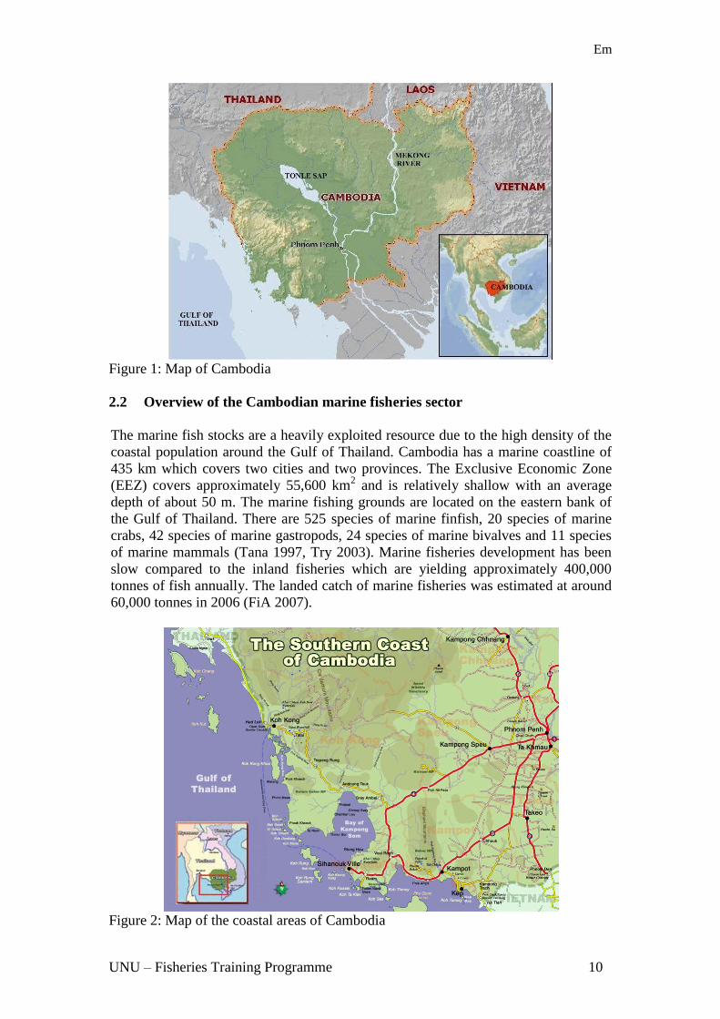
Em
UNU ndash Fisheries Training Programme 10
Figure 1 Map of Cambodia
22 Overview of the Cambodian marine fisheries sector
The marine fish stocks are a heavily exploited resource due to the high density of the
coastal population around the Gulf of Thailand Cambodia has a marine coastline of
435 km which covers two cities and two provinces The Exclusive Economic Zone
(EEZ) covers approximately 55600 km2 and is relatively shallow with an average
depth of about 50 m The marine fishing grounds are located on the eastern bank of
the Gulf of Thailand There are 525 species of marine finfish 20 species of marine
crabs 42 species of marine gastropods 24 species of marine bivalves and 11 species
of marine mammals (Tana 1997 Try 2003) Marine fisheries development has been
slow compared to the inland fisheries which are yielding approximately 400000
tonnes of fish annually The landed catch of marine fisheries was estimated at around
60000 tonnes in 2006 (FiA 2007)
Figure 2 Map of the coastal areas of Cambodia
Em
UNU ndash Fisheries Training Programme 11
221 Marine catches
The Department of Fisheries statistics (2004) cited by the Community Fishery
Development Office (CFDO 2005) reports that the annual marine catches were
estimated at about 36000 tonnes in 1994 ndash 2000 This number excludes the catches of
subsistence and illegal foreign fishing The Fisheries Administration has estimated the
increase in fish production from 36000 tonnes in 2000 to 60500 tonnes in 2006
(Table 2) which includes catch in mangrove areas due to the fact that the harvest of
mangroves is covered by the present fisheries law
In fact the actual catch of marine fisheries is higher than the official statistics suggest
This is because the catches from subsistence fishing including family-scale fisheries
are largely unrecorded Furthermore catches from illegal fishing activities are not
recorded Csavas et al (1994) state that information on the landing of marine fish in
Cambodia can be inferred from records of fish landings from the Thai portion of the
Gulf of Thailand This is partly due to the Thai vessels fishing in Cambodian waters
and some Cambodian fishing boats selling or transferring their catch to Thai mother-
vessels at sea or landing in Thai ports According to the DoF internal reports catches
from licensed Thai vessels in Cambodian water are estimated to be from 26500
tonnes to 37500 tonnes (Gillett 2004) Robert (Gillett R 2004) also concluded that if
this is indeed the case this amount would approach the total marine catch recorded for
all Cambodian fishing vessels operating offshore Substantial Thai catches in
Cambodian waters complicate any management strategy for Cambodian fish resources
because of difficulties associated with ensuring that rents from improved Cambodian
management actually benefit Cambodian fishermen and not only the less regulated
Thai fishing fleet
The marine fishery involves coastal fishers in inshore areas and foreign fishers
operating legally and illegally in offshore areas (NACA 2004) Cambodia currently
does not have the capacity to exploit offshore areas Since 1992 marine fisheries
statistics have included estimates of catches by foreign fishers licensed to operate in
the EEZ of Cambodia (DoF 2001d)
Table 2 Total fishery production inland and marine fishery from 2000-2006 (FiA
2007)
Year Total
(tonnes)
Inland (ton) Marine
(tonnes) Total Commercial
fisheries
Familysubsist
ence fisheries
Rice field
fisheries
2000 281600 245600 85600 110000 50000 36000
2001 427000 385000 135000 140000 110000 42000
2002 406150 360300 110300 140000 110000 45850
2003 363500 308750 94750 120000 94000 54750
2004 305800 250000 68100 106400 75500 55800
2005 384000 324000 94500 137700 91800 60000
2006 482500 422000 139000 181000 102000 60500
222 Catch by species and finfish production
Finfish is the main group of annual total catches by year (Table 3) Try (2003)
indicated that 33 species of finfish are commonly exploited Only five species are
very abundant in the landings Megalaspis cordyla (torpedo scad) Scomberomorus
commersoni (narrowbarred Spanish mackerel) Rastrelliger brachysoma (short
Em
UNU ndash Fisheries Training Programme 12
mackerel) Rastrelliger kanagurta (Indian mackerel) and Atule mate (yellowtail scad)
The volume of finfish caught in 2006 decreased slightly compared to 2005 but the
total catches have increased in 2006 as Anadromous fish (3678 tonnes) were not
record in 2005
The catches of trash fish each year rank the second after finfish (Table 3) In 1960 the
trawl gear was introduced to fishers in Cambodia that allows for catch of demersal
fish and juveniles During the past three decades trash fish was discarded due to no
demand and no value in the market But after 1993 a factory was built in Sihanoukvill
for processing trash fish for fish feed Therefore fishers catch and collect the trash
fish resulting in that the volume of trash fish has recently increased
As the market price of economic fishes has gradually been increasing trash fish have
become food for local people and particularly the poor coastal dwellers who have a
low income According to Try (2006) it was estimated that the trash fish caught by
trawl in 1980 is about 30-40 of the total catch but the percentage of trash fish was
recently increased probably to 60-65 of marine fish catches by trawl It seems that
to be encouraging the fishers use a more efficient gear to fish in inshore waters than
offshore Perhaps they are also using illegal fishing gears such as trawlers mosquito
net push and small mesh sizes of nets catching all fish species and sizes The marine
fish catches in 2006 have declined for all groups except shrimp from 2005 (Table 3)
Table 3 Statistics of marine fisheries caught by groups in Cambodian coastal waters
(in tonnes) (Try et al 2006 and FiA 2007)
Yea
r
Fin
fish
Tra
sh f
ish
Sh
rim
p
pra
wn
s
Ray
s
Sq
uid
cutt
lefi
sh
Lo
bst
ers
Cra
bs
Gas
tro
po
ds
Sea
slu
g
An
adro
mo
us
fish
To
tal
mar
ine
fish
ery
2000 15526 9833 2905 245 2627 59 3593 801 11 410 36010
2001 16873 10847 3872 209 2355 40 3462 3681 0 661 42000
2002 18910 11752 3827 553 2681 122 3545 3007 3 1410 45810
2003 26596 14859 4055 727 3577 169 4028 648 2 61 54722
2004 25639 16570 3824 620 2984 124 3458 2457 0 124 55800
2005 26141 18265 4124 996 3723 1233 4301 1215 2 0 60000
2006 25641 17194 4778 476 3551 115 4180 897 0 3678 60500
Almost 90 of the marine fisheries production in Cambodia is from two coastal
provinces Sihanoukvill and Koh Kong (Table 4) The total catches of finfish are
mackerel fish amount 4650 tonnes (FiA 2007) The trash fish is second in rank
among the group species caught of which Koh Kong and Sihanoukvill rank at the top
Table 4 Statistics of marine product of four main coastal areas 2006 (FiA 2007)
Cit
y
pro
vin
ce
Fin
fish
Tra
sh f
ish
Sh
rim
p
pra
wn
s
Ray
s
Sq
uid
cutt
lefi
sh
Lo
bst
ers
Cra
bs
Gas
tro
po
ds
An
adro
mo
us
fish
To
tal
mar
ine
fish
erie
s
Kampot 2103 1674 386 32 130 5 635 415 2000 7380
Kep 300 - 35 5 10 - 45 17 18 430
Koh Kong 13519 10500 1622 89 1100 - 2000 280 160 29270
Sihanoukvill 9709 5020 2735 350 2311 110 1500 185 1500 23420
Total 25631 17194 4778 476 3551 115 4180 897 3678 60500
Em
UNU ndash Fisheries Training Programme 13
223 Costal fishers and employment
Most coastal fishers are poor and generally use small-scale fishing gear that is only
adequate for use inshore and in mangroves There are limited numbers of coastal
fishers that have sufficient capital to invest in the necessary vessels and gear for
offshore fishing The capacity of fishers fishing offshore in the EEZ is not large
compared to the potential exploitation
Officially the statistics of fisheries employment have shown only the number of
people involved in fisheries harvesting processing and culturing There are no
statistics on other numbers of people employed in fisheries related activities The
number of fishers and the number of fish processor is reflected in Table 5 below
Table 5 Statistics of fishers and processors 1999-2006 (DoF‟s Statistics 2000-2006) Year Harvesting labour force in marine sector
Processing labour
force Familyrice field
Mobileartisanal
Fisheries Total fishers
No of
families
No of
fishers
No of
families
No of
fishers
No of
families
No of
fishers
No of
families
No of
processors
1999 0 0 3910 11721 3910 11721 373 1527
2000 0 0 6557 14647 6557 14647 379 1631
2001 6445 8067 4137 15350 10582 23417 370 1499
2002 24818 45940 9648 26130 34466 72070 1472 2379
2003 16047 28638 13159 40014 29206 68652 990 1815
2004 16475 31657 10865 33274 27340 64931 1407 4234
2005 - - - - - - - -
2006 18949 37990 12006 36582 30955 74572 1226 29412
224 Number of vessels
Non-motorised and motorised vessels are used in Cambodia‟s marine fisheries Most
non-motorised vessels are used by the small-scale fishers who carry out subsistence
fishing The Fisheries Department has statistically categorised the non-motorised
vessels based on their dead weight The three categories are less than 5 tonnes more
than 5 tonnes and Duk-boats but the Duk-boat is not directly used for fishing (ie it
is used for transporting the fisheries products)
The motorised vessels are divided into four categories based on engine power less
than 10 hp 10 to 30 hp 30 to 50 hp and more than 50 hp This classification does not
include data on the number of vessels involved in small-scale and large-scale
fisheries
The number of non-motorised vessel in 2000 was only 255 and increased to 841 boats
in 2002 operating within Cambodia‟s coastal zone then it dropped dramatically to
272 boats in 2004 and increased again to 821 boats in 2005 and 1059 boats in 2006 as
illustrated in Figure 3
Noticeably the number of motorised fishing vessels seems to increase linearly from
5037 boats in 2000 to 7027 boats in 2005 and drop to 6236 boats in 2006 Most of
the motorised fishing vessels with large fishing gears are required to have licenses to
operate Two systems exist of motorised fishing vessels licenses one is a license
issued by the provincial fisheries office for all motorised vessels equipped with engine
Em
UNU ndash Fisheries Training Programme 14
power under 33 horse power (hp) and another is a license issued by the Fisheries
Administration for all motorised vessels equipped with an engine power above 33
horse power (hp)
Referring to regulations on offshore and inshore vessels it can be assumed that all the
motorised vessels which have small engine power (below 50 hp) and non-motorised
vessels operate inshore Motorised vessels equipped with engine power greater than
50 hp should operate offshore
Fishing vessels equipped with engine power higher than 50 hp may use a labour force
from 5 to 15 people depending on the fishing gear used For boats with an engine
power higher than 100 hp the labour force may be 15 to 30
Figure 3 Number of marine fishing vessel from 2000-2006 (FiA 2007)
225 Annual contribution of marine fisheries to the economy
According to a government report the marine capture fishery has increased from
36000 tonnes in 2000 to 60500 tonnes in 2006 (Table 2) Thus the average marine
capture fishery was around of 50700 tonnes per year from 2000 to 2006 Try et al
(2006) mentioned that the average market price of marine fish is US$ 1 per kg The
marine capture fishery can be estimated to value US$ 507 million a year at the
market site If the tourism industry in Cambodia shows a steady increase of 20
yearly (MoT 2007) the demand for food consumption for tourists will increase This
leads to an increase in the domestic market price of marine fish in Cambodia and the
marine capture fisheries in 2006 can be estimated to value in total revenue around
US$ 635 million According to Try et al (2006) the capture marine fishery values
account of US$ 15 million to US$ 30 million excluding the illegal export which is
un-reported This estimation was at the average market price of trashfish at 500
Cambodian Riels per kg The share of fisheries in the GDP or government revenue
was 108 in 2000 and the estimate for 2005 is 930 (Table 1)
226 Fisheries landing ports
Landing locations are not separated from fishing locations and harbour facilities are
limited Much of the catch is transferred to Thai vessels at sea for landing in Thailand
(FAO 2005) Landing sites of four main coastal areas are used for statistics a total of
about 131 locations landings exist in Sihanoukvill 69 Koh Kong 55 Kampot 4 and
Em
UNU ndash Fisheries Training Programme 15
Kep City 3 Most landing ports are small and rural services and facilities are poor It
may be concluded that fishery landing ports of four main coastal provinces are not of
interest to the private sector to invest in rather these are subsidised by the
government
23 Mackerel fisheries
Mackerel consists of commercial pelagic groups which include short mackerel Indian
mackerel Indo-Pacific mackerel Spanish mackerel and island mackerel They are the
most important pelagic species in the Gulf of Thailand harvested by commercial and
traditional gears The local name ldquoPlathu Kamongrdquo is used loosely to refer to all
these fish species
231 Mackerel production
The highest recorded annual landing of mackerel (Rastrelliger) was 139220 tonnes
and contributing 14 to all the marine fish landed in 1968 in the whole Gulf of
Thailand Second to this 122156 tonnes or 11 of the marine fisheries landings were
recorded in 1969 (Sea Around Us 2005) These species supported the purse seine and
gillnet fisheries since the early 1960s and have remained important until now In fact
mackerel is the most dominant commercial food fish in the Gulf of Thailand
The catch of mackerel declined from about 40000 tonnes in the 1950s to around 20000
tonnes in the 1980s An unusually sharp increase in catch occurred though in 1965-1971
when the catch reached 140000 tonnes The pressure from the industry in Thailand has
resulted in overexploitation Ahmed et al (2007) state that ldquofor a number of decades
fisheries development in the Gulf of Thailand has concentrated on increasing fishing
effort to maintain or increase the production volumerdquo Most important pelagic fish in
the Gulf of Thailand are fully exploited especially Indo-Pacific mackerel anchovies
round scad and sardines and demersal resource stocks are over-fished (FAO 1995)
Figure 4 Volume of mackerel caught in the Gulf of Thailand from 1950-2004 (Sea
Around Us 2005)
232 Mackerel fisheries exploitation and its catch effort in Cambodia
Mackerel is not only sold on the domestic market but is also exported to Thailand
every year both fresh and processed Mackerel in Cambodia is caught by artisanal
fishermen as well as the industrial fishery The artisanal fishery operates from small
Em
UNU ndash Fisheries Training Programme 16
boats with outboard engines of less than 33 hp Most of these fishing boats use
gillnets to catch in inshore areas The industrial mackerel fishery is operates offshore
using purse seines or driftnets with boat engines up to 50 hp The commercial fishing
boat can stay at sea fishing 2 to 5 days This type of boat has facilities to keep fish for
long time
Since 1990 the catch of mackerel by Cambodia had increased from about 1000
tonnes to 4650 tonnes in 2006 (Table 6) From 2002 to the present the catch has been
stable at around 4500 tonnes but the effort has increased with a corresponding
reduction in CPUE
The gillnet boats fish for mackerel approximately 25 days a month 8 months a year
The purse seine operates only during the dry season period of 5 months (20 days per
month) The purse seine boats have crews of about of 15 to 30 people The gillnet
boats can on the other hand operate with a labour force of only 2 to 3 people
Table 6 Volume caught fishing effort and CPUE of mackerel from 1990-2006 (FiA
2007)
Year
Catches
volume
(tonnes)
Fishing effort CPUE
(Kgperson
day)
Boat used gillnet Boat used purse seine Total
boat
Total
labour Boat Labour
(person) Boat
Labour
(person)
1990 1395 - - - - - - -
1991 1212 - - - - - - -
1992 1101 3 9 13 260 16 269 40
1993 1424 9 27 14 280 23 307 43
1994 1513 31 93 15 300 46 393 31
1995 1683 10 30 16 320 26 350 44
1996 1452 14 42 6 320 30 362 36
1997 1278 114 342 15 300 129 642 13
1998 1447 122 366 15 300 137 666 14
1999 1738 172 516 8 160 180 676 15
2000 1559 155 465 10 200 165 665 14
2001 1731 56 168 10 200 66 368 32
2002 4300 50 150 10 200 60 350 86
2003 4421 73 219 13 260 86 479 63
2004 4764 117 351 10 200 127 551 53
2005 4906 250 750 4 80 254 830 31
2006 4650 181 543 6 120 187 663 39
233 Mackerel fish processing products
The mackerel in Cambodia is traditionally processes by salted or steaming For
steamed fish ldquoshort body mackerelrdquo is the local name called as Trey Chom Houy but
for salting ldquoSpanish mackerelrdquo is used the local name is Trey Borb Most production
is for the domestic market Data is limited on export
234 Marketing and price of mackerels
Locally the price of mackerel and its products can be different between markets
throughout the land However the difference between the markets of the four
Cambodian coastal areas is small The Sihanoukville market site is the main
Em
UNU ndash Fisheries Training Programme 17
distribution centre of marine fisheries products into the local market thus the market
price of Mackerel fishes and its products in Sihanoukvill can be assumed as the local
market standard price of Mackerel fishes and its products According to monthly
reports of the Marine Fishery Division the price of mackerel at the landing site and
domestic market is actually increasing especially in the wet season when catch is
small and but demand is high
In 2006 the price of short mackerel at the landing site from January to September
fluctuated from US$ 450 to US$ 625 per tonne1 (Figure 5) Based on data estimated
by the Fishery Administration the landing volume of mackerel species in 2006 was
about 4650 tonnes and can be estimated at around US$ 252 million or 4 of the
marine fishery revenue in 2006 Spanish mackerel is selling at a high price at the
landing and market site but the landing volume is small compared to short mackerel
The landing price of Spanish mackerel within a 9 month period in the year 2006
fluctuated increasingly from US$ 1375 to US$ 3500 per tonne Figure 5 illustrates
the price of short mackerel and Spanish mackerel correlated at two sites domestic
market and local landing site
In general the price of marine fish at landing as well as market site has increased over
the years due to an increase in the fishing operational cost Moreover increased
population leads to high market demand for human consumption whereas the natural
resources are gradually decreasing Thuok et al (2001) stated that marketing channels for
marine products are not so well developed for food security and economy reasons it is
believed that emphasis should be placed by the administration in support of the private sector
on the development and enhancement of marketing of marine fishery products
Figure 5 Price of mackerels at landing and market site for 9 months in 2006 (FiA
2007)
1 The price of mackerel at landing site was conducted and reported to the Fishery Administration by Marine
Fishery Division from January to September in 2006
Em
UNU ndash Fisheries Training Programme 18
24 Marine fisheries resources management in Cambodia
241 Law and regulation
The Cambodian marine fishery is managed under the Fisheries Law of 2006 which is
an improved and updated version of the law from 1987 The main objective of the law
and regulation is to manage and conserve the marine fishery resources in a sustainable
manner Additional objectives are to generate governmental revenue improve the
livelihood of local communities and achieve ecologically sound management by an
improved statistical system gear restrictions area limitations and time closures
Management objectives other than those in the Fishery Law 2006 exist and are
attained by the Ministry of Agriculture Forestry and Fishery (proclaim issue) ie
closed season from 15 January to 31 March for mackerel species
For management purposes the marine fisheries are divided into two groups
Coastal fisheries small family-scale fishing operating in fishing zone 1 which
extends from the coast to a depth of 20 m this fishing zone was almost managed by
community fisheries The coastal community fisheries were established after the
government recognised the poor management of the fisheries sector which resulted in
a movement for reform in 2000 Nowadays 40 community fisheries have been
established along the coast to encourage coastal dwellers to participate in the
management of their resources Fishers use boats without engines or with engines of
less than 50 hp Licenses are not required for boats with no engine or with engines
below 33 hp but for boats with more than 33 hp engines a license fee of 27000 Riels
(US$ 7) per horsepower per year is required Fishing activities are not allowed to
include other fishing gears such as trawls or light fishing
Commercial fisheries refer to large-scale fishing from 20 m depths to the limits of the
EEZ Boats used have engines with more than 50 hp which must be licensed for a fee
of 27000 Riels (US$ 7) per horsepower per year Prohibited fishing gears and
methods include pair trawling light fishing and other illegal fishing gears All marine
fisheries are open year round apart from mackerel for which fishing is banned from
15 January to 31 March (DoF 2001d) Most of the small boats (engine lt 50 hp)
marine fishing fleets use alternative multi-fishing practices following the seasonal
appearance of marine resources including purse-seines gill nets push nets and
trawling Foreign poachers use prohibited gears such as large bottom trawls long drift
nets pair trawlers light fishing and explosives (DoF 2001d)
242 Management and administration
Despite a few limitations on the fisheries in the Gulf of Thailand fisheries there fall
under the framework of unregulated open access In addition there are no limits
placed on the amount of gears that can be used the amount of time that can be spent
fishing or on the quantity of fish that may be captured
Generally coastal fishers can operate all year round by using many different types of
fishing gears However the use of fishing gears is dependent on a number of critical
factors including (1) the capital invested (2) experience and traditions of the fishing
communities in different locations along the coast (3) seasonal abundance of different
Em
UNU ndash Fisheries Training Programme 19
species (4) seasonal weather conditions and (5) ecological conditions associated with
the fishing grounds (eg inshore offshore mangrove coral reef etc)
Fishing in offshore areas is still a challenge and there is a lack of strong law
enforcement measures against illegal fishing from neighbouring countries It is a
problem represented in the low annual production of marine fisheries The present
management of data collection is not sufficient to develop plans for scientific
management of marine fish stocks The lack of knowledge of fish biology ecology
and their dynamics results in a poor understanding of the recent changes in marine
fish stocks (MAFF-DoF 2004)
On the other hand the fisheries competency is still inadequate This is true in terms of
inspection specialists and the lack of adequate physical means to enforce legislation
such as protection against illegal fishing (ie the Fisheries Administration is less able
to set up or install the right technology a high speed boat radio communication and
other facilities for coast guard operations) Furthermore in the 1990s the political
environment was unstable which affected the business environment and led to less
investment capital
However the government and Fisheries Administration have overcome many
obstacles to develop and manage marine fisheries resources as well as the fisheries
sector in the past years Especially a recent achievement is the Fishery Law
completely promulgated public using in 2006 (FiA 2007) The new law was updated
from the previous Fishery Law of 1987 which was based on legislation from 1956
1958 and 1960 (revised) The updated law was also drafted with participation from
stakeholders IOs NGOs and relevant partners through research study and sustainable
development projects on the fisheries sector framework In terms of gains marine
production through fishing effort as well as improve capacity of fishing and biomass
management in EEZ
3 THE PRINCIPLES OF FISHERIES MANAGEMENT
This chapter has been adapted from the lecture notes in the UNU-FTP specialist
course on Fisheries Policy and Planning by Prof Ragnar Arnanon
The need for fisheries management stems fundamentally from the fact that fish
resources are common property It is well known both from theory and experience
that common property resources will be overexploited and possibly irreversibly
depleted unless subjected to appropriate fisheries management Essentially the
fisheries management regime is a set of social prescriptions and procedures that
control the fishing activity Similarly fisheries management requires either collective
action at the industry level or external usually government intervention
The principles of fisheries management or fisheries management regimes consist of i)
the fisheries management system (FMS) ii) monitoring control and surveillance
(MCS) and iii) fisheries judicial system (FJS) These three components of the
fisheries management regime are strongly interdependent All three components of the
fisheries management regime are crucial to its success They are links in the same
chain If one of them fails the fisheries management regime as a whole fails
Em
UNU ndash Fisheries Training Programme 20
31 The fisheries management system (FMS)
The fisheries management system specifies the regulatory framework for the fishing
activity It consists of all the rules that the fishing activity must obey such as gear and
area restrictions fishing licences catch quotas etc In many countries most fisheries
rules are based on explicit legislation In others they are primarily based on social
customs and conventions
The fisheries management system is basically a set of rules about how the fishery
should be conducted These rules may be formal ndash for instance in the form of
published laws and regulations ndash or they may be informal ndash a part of the social culture
governing fishing behaviour In most fisheries both types of fisheries management
rules the formal and the informal apply The purpose of the fisheries management
system is to contribute to the generation of net economic benefits flowing from the
fishery
The fisheries management represents the application of specific fisheries management
instruments or tools Typical fisheries management tools are for instance fishing gear
restrictions limitations on the number of allowable fishing days during the year area
closures and so on Thus the fisheries management tools are like variables or more
precisely control variables and the fisheries management measures the values that can
be chosen for these control variables
Now fisheries management systems consist of particular combinations of one or more
of these tools Thus obviously the number of possible fisheries management systems
increases very fast with the number of available fisheries management systems Most
of them may however be grouped into two broad classes i) Direct fisheries
management and ii) indirect fisheries management as illustrated in Figure 6
Figure 6 Fisheries management systems a classification (adapted from lecture notes
UNU-FTP 2007 introduced by professor Arnason)
Direct fisheries management attempts to control the components of the fishing
activity directly by commands or more often restrictions that must be adhered to
Indirect economic fisheries management by contrast attempts to induce the fishing
firms to behave differently by modifying the operating conditions of the fishery
without imposing direct constraints The difference between direct biological and
economic fisheries management lies in what they seek to control Direct biological
fisheries management attempts to alter the biological yield of the fishery Thus under
biological fisheries management for instance the sustainable yield curve is normally
shifted Direct economic fisheries management attempts to alter the behaviour of the
Em
UNU ndash Fisheries Training Programme 21
fishing firm days vessel size etc Thus direct economic management generally
affects the cost structure of the fishery directly
Indirect fisheries management alters the operating conditions of the fishing industry
There are of course many ways to do this Most however belong to two main
categories (a) taxes (and subsidies) which basically alter the prices facing the fishing
industry and (b) property rights which alter the nature of the external effects imposed
by the fishing firm on one another
Most fisheries management tools are fall quite naturally into one of the fisheries
management categories in Figure 6 The main exception is the total harvesting
restriction or total allowable catch (TAC) Of all the fisheries management systems
considered above only (i) certain property right arrangements and (ii) tax on catch
seem to be theoretically capable of delivering the full potential economic benefits of
fisheries Direct fisheries management irrespective of whether it is based on
biological or economic restrictions seems particularly inept for this purpose
Em
UNU ndash Fisheries Training Programme 22
32 Monitoring control and surveillance (MCS)
The primary task of the monitoring control and surveillance system is to observe the
fishing industry‟s activities and to enforce its adherence to the rules of the fisheries
management system Its secondary but nevertheless very important task is to collect
data about the fishery that can be used to improve both the fisheries management and
fisheries judicial system as well as the monitoring control and surveillance system
itself Broadly speaking the phrase refers to two activities i) the monitoring of the
fishery and the activities of the fishing (harvesting) industry and ii) the enforcement
of fisheries management rules
MCS is as already discussed a crucial component of any fisheries management
regime Logically it is the management authority that must conduct and co-ordinate
the MCS activity although it may engage contractors it is the central fisheries
manager ie the government that operates the MCS activity
The monitoring part of MCS involves collection of the relevant biological data about
the fish stocks and the surrounding ecosystem as well as the relevant technical
economic and behavioural data about the fishing industry and its activities The
monitoring activity is conducted for essentially two purposes i) to gather information
for improving the fisheries management ie data generation monitoring and ii) to
gather information for the purpose of enforcing existing fisheries management rules
ie enforcement monitoring It is important to realise that in order to transform
fisheries data into sensible decisions on fisheries management measures and
modifications of the fisheries management system a good deal of biological and
economic research has to take place Hence is should be clear that research both
biological and economic is an integral part of the monitoring part of the MCS
activity
The enforcement part of MCS consists of acting upon alleged violations of fisheries
management rules It generally takes place where and when the violating activity
occurs The action taken may be of several degrees of severity i) induce the violator
end the illegal activity ii) impose a penalty ie an administrative penalty typically a
fine or a temporary revoking of fishing licence iii) indict the alleged violator and iv)
apprehend and indict the alleged violator In this case the alleged violator is
apprehended (a penalty in itself) and also formally charged for the offence
It should be clear that if the fishing firms are profit maximisers enforcement action
will in general not suffice to generate sufficient adherence to the fisheries
management rules unless the level of monitoring and enforcement is extremely
highly relative to the fishing activity Since the former implies that a decentralised
fishery can never be efficient and the latter is obviously far too expensive compared to
the value of the fishery we may conclude that any reasonable MCS system must rely
on (ii)-(iv) to a significant extent For later reference it is useful to note that the
enforcement part of MCS especially degrees (iii) and (iv) above is linked to the
operations of the fisheries judicial system and in fact depends on it if it is to be
effective
The cost of MCS in fisheries is by no means negligible The available indications
(Arnason et al 2002) suggest that this cost usually ranges between 2 and 10 of
Em
UNU ndash Fisheries Training Programme 23
the total landed value of national the fisheries According to Arnason et al (2002) the
most important MCS cost items appear to be i) enforcement at sea and on land ii)
data collection and research and iii) policy formulation and system administration
Enforcement costs especially those at sea are generally very high and as a whole
usually account for well over half of the total MCS costs Data collection and research
costs typically account for over a third of the total MCS costs with the most costly
item being biological research The rest of MCS costs are accounted for by policy
formulation and general administration costs
33 Fisheries judicial system (FJS)
The fisheries judicial system is part of the general judicial system It should be noted
however that in most societies the formal judicial system is to process alleged
violations of fisheries management rules and issue sanctions to those deemed to have
violated the rules The fisheries judicial system thus complements the monitoring
control and surveillance activities in enforcing the fisheries management rules
The purpose of the fisheries judicial system (FJS) is to i) process alleged violations of
fisheries rules and ii) apply sanctions as appropriate It follows that the FJS must
contain well defined procedures as to how to process alleged violations What are the
courts how may cases be referred to the courts what are the appeal procedures time
limits and so on Without the support of the fisheries judicial system the MCS
activity would not work Alleged violators would simply go to court and get off with
penalties insufficient to deter them from their illegal activities Hence the MCS
activity would be of little use In particular it would not succeed in enforcing the
fisheries rules
It is often found that the fisheries judicial system is the weakest link in the fisheries
management regime The public information and awareness of the judicial system is
not well distributed and the people then are not well-informed Fundamentally the
judiciary system is fairly independent of the executive and legislative branches of
government As a result the fisheries management regime is much less amenable to
reform and change than the other two components The trials and judgements are
passed according to law custom and convention The judicial system in executing
laws and judgements generally has little understanding of the intricacies of the FMR
This suggests the need to include carefully designed laws concerning the treatment of
fisheries violations the burden of proof penalties etc in the fisheries legislation
defining the fisheries management regime
The main objective of the FJS is to endorse the enforcement part of the MCS activity
In particular the FJS determines crucial components of the probability that a violator
of fisheries legislation will suffer penalties The adherence to fisheries management
rules requires sufficiently high administrative costs in processing these allegations
Generally any expected cost of violations can be generated by the appropriate
combination of enforcement and penalties To find this appropriate combination it is
necessary to obtain an empirical estimation from the increased enforcement activity
and improved FJS and its implications to the expected costs of violations
Em
UNU ndash Fisheries Training Programme 24
4 MODELLING
The bio-economic model applied in this chapter has been adapted from the lecture
notes in the UNU-FTP specialist course on Fisheries Policy and Planning by Prof
Ragnar Arnanon
The model applied in this report is used to explain the mackerel fishery in Cambodia
and investigate improvements in its utilisation it is a simple bio-economic model of
the fishery resources The model chosen is based on the work of Gordon (1954) and
Schaefer (1957) (Anderson G L 1981) who developed a basic bio-economic model
for fisheries management The main elements of this model are i) a biomass growth
function which represents the biology of the model ii) a harvest function which
constitutes the link between the biological and economic part of the model and iii) a
fisheries profit function which represents the economic part Particularly for
prediction of the maximum sustainable yield (MSY) of the mackerel fishery we apply
the ldquosurplus production modelsrdquo a simple model introduced by Graham (1935)
(Anderson G L 1981) but they are often referred to as ldquoSchaefer modelsrdquo This
approach was selected for the following reasons i) the Cambodian mackerel fishery
data is very limited and thus does not support an advanced bio-economic model ii)
the model developed here can later be extended and refined when more and better
data becomes available More precisely the model is as follow
x = G(x) ndash y (Biomass growth function) (1)
where x represents biomass x is biomass growth and y is harvest The function G(x) is
natural biomass growth
y = Y(ex) (Harvesting function) (2)
The volume of harvest is taken to depend positively on fishing effort as well as the
size of the biomass to which the fishing is applied
π = p∙Y(ex) ndash C(e) (Profit function) (3)
Where p represents the price of fish landing and C(e) is the cost function of fishing
effort The profit function depends on the fish price the sustainable fish yield and the
fishing operation costs The fishing costs depend on the use of economic inputs
which is the fishing effort can represent the profit function equation
The above model comprises three elementary functions the natural growth function
G(x) the harvesting function Y(ex) and the cost function C(e) It adopts the widely
used specific form for these functions
41 The biomass growth function
Populations of organisms cannot grow infinitely the growth of organisms is
constrained by environmental conditions and food availability It has been shown that
populations of organisms strive to stabilise at the highest possible population size for
a given set of conditions (Schaefer 1954) (Anderson G L 1981) Marginal growth of
a population increases when the size of the population decreases and marginal growth
Em
UNU ndash Fisheries Training Programme 25
decreases when the size of the population increases this may be called density
dependent growth Biological growth of such populations may be expressed as
follows
G(x) = rx ndash sx2 (4)
Where x is population size r is the growth rate of the population and s is the mortality
rate which is negative This is the parabolic equation also referred to as Verhults‟
equation or the logistic growth equation (Schaefer 1954) (Anderson G L 1981)
When the population reaches the environmental carrying capacity (K) growth and
mortality of the population is equal and rate of change of population size with respect
to time (dxdt) becomes zero The mortality rate s can now be expressed in terms of r
and K as
(5)
From equation (5) substitute s in equation (4) we get the most commonly used
expression of the logistic growth equation and equation (4) can be rewriten as
(6)
Fox (1970) (Arnason R 2007) outlined an alternative surplus yield model assuming
the Gompertz growth function resulting in an exponential relationship between
fishing effort and population size and an asymmetrical harvest curve (Fox 1970)
(Arnason R 2007) The generalised form of the Gompertz curve can be represented
as (Winsor 1932) (Arnason R and Bjorndal T 1991)
F(x) = micro∙x(lnK ndash lnx) (7)
In this formulation the carrying capacity of the biomass is K as in the logistic
formulation However unlike the logistic the Fox-Gompertz growth function is not
symmetric and the intrinsic growth rate is infinite compared to r for the
logistic
The major difference between the logistic model and the Fox model is that at lower
population sizes the Fox model predicts a higher growth rate than the logistic model
At higher population sizes the logistic model predicts a higher growth rate than the
prediction by the Fox model In the logistic model maximum growth occurs at half of
the maximum population level In the Fox model maximum growth occurs at a
population level of less than the half of the maximum population around 37 of the
maximum population On the other hand the population growth curve of the Fox
model is skewed to the left while the population growth curve of logistic model is
symmetrical
Em
UNU ndash Fisheries Training Programme 26
Figure 7 Illustrates the logistic biomass growth model G(x)
Figure 8 Illustrates the Fox biomass growth model G(x)
For biomass growth we consider the logistic and the Fox
G(x) = α∙x - β∙x2
(8)
F(x) = α∙x - β∙ln(x)∙x (9)
42 The harvesting function
Assuming that each unit of effort harvest equals the amount from the targeted stock
and an equilibrium situation where catch equals natural growth the equilibrium stock
size (x) may be expressed in terms of carrying capacity (K) catchability coefficient
(q) and fishing effort (e) For the harvesting model in accordance to the generalised
Schaefer (1954) (Anderson G L 1981) version
Y(ex) = q∙e∙xb (10)
Where the coefficient b indicates the degree of schooling behaviour by the fish which
b Є[01]
43 The cost function
Consequently the costs of fishing effort will be a linear function of the amount of
effort ndash index of economic input in the form of labour investment fuel maintenance
and supplies fixed costs and overhead that is devoted to the fishery on an annual
basis The annual cost of fishing C(e) is proportional to effort (e) For this report it
was assumed that the fishing boats are homogeneous The cost function is expressed
as
Em
UNU ndash Fisheries Training Programme 27
C(e) = c∙e + fk (11)
Where c represents marginal costs and fk represents fixed costs
44 The complete model
The complete model based under those function specifications becomes
Biomass growth function
- = α∙x - β∙x2 ndash y (Logistic) (12)
- = α∙x - β∙ln(x)∙x ndash y (Fox 1970) (13)
Harvesting function
- y = q∙e∙xb (14)
Profit function
- π = p∙y ndash c∙e + fk (15)
The last two equations can be combined to yield a simpler version of the model
- π = p∙y ndash(cq)∙y∙x-b
+ fk (16)
The ratio (cq) is viewed as a single parameter known as the normalised marginal cost
It is shown that the marginal cost and catchability c and q are not displayed in an
independent role in this model What counts in the model is the ratio of the two
constant parameters
45 Sustainable yield
The annual rate of renewal of fish stock depends on three major factors biological
environment physical environment and magnitude of the remaining population
Biological and physical environment may be considered to be constant in the long run
(Schaefer 1954) (Anderson G L 1981) Population size is reduced by natural and
fishing mortality Harvesting increases the total mortality As the fish population
strives to balance the total mortality with growth the population reaches a new
equilibrium at a point where the growth rate equals total mortality which occurs at a
lower population size than the environmental carrying capacity level K When the fish
stock reaches equilibrium with a given effort level all biological growth of the
population is harvested and there is no need for change in the population size
y(ex) = G(x) (17)
(18)
and when
Em
UNU ndash Fisheries Training Programme 28
(19)
by substituting x in the equation (18) with equation (19) we get the long term catch
equation
(20)
This implies that although harvest is a function of effort and stock size for the short
term in the long run stock size becomes only a function of effort (given that
environmental conditions are constant) and the sustainable yield too becomes a
function of effort only
Equation (8) takes the form of a parabolic equation which allows us to use linear
regression in order to estimate the parameters of the function of sustainable harvest
(y) Dividing both sides of equation (8) by effort (e) we get the linear equation of
catch per unit effort (CPUE)
(21)
Assuming that biological growth of the subjected population follows the model
suggested by Gowpertz and also assuming the fleet is homogenous and all vessels
have the same fishing power
(22)
by substituting x in equation (6) with (22) the equation became as below
(23)
Dividing both sides of equation (23) by fishing effort (e) yields
(24)
A long-linear expression is found by
(25)
46 Maximum sustainable yield (MSY)
The objective of the application of the ldquosurplus production modelsrdquo is to determine
the optimum level of effort that is the effort that produces the maximum yield that can
be sustained without affecting the long-term productivity of the stock the so-called
maximum sustainable yield (MSY) Because holistic models are much simpler than
analytical models the data requirements are also less demanding There is for
example no need to determine cohorts and therefore no need for age determination
Em
UNU ndash Fisheries Training Programme 29
This is one of the main reasons for the relative popularity of surplus production
models in tropical fish stock assessment Surplus production models can be applied
when data are available on the yield (by species) and of the effort expended over a
certain number of years The fishing effort must have undergone substantial changes
over the period covered The basic models were expressed as follows
461 Surplus production models
The maximum sustainable yield (MSY) can be estimated from the following input
data
- f(i) = effort in year i where i = 1 2 3 hellip n
- Y(i) = yield in year i where i = 1 2 3 hellip n
- Yf = yield (catch in weight) per unit of effort in year t
Yf may be derived form the yield Y(i) of year i for the entire fishery and the
corresponding effort f(i) by
(i) Yf = Y(i) f(i) where i = 1 2 3 hellip n (26)
The simplest way of expressing yield per unit of effort Yf as a function of the effort
f is the linear model suggested by Schaefer (1954) (Anderson G L 1981)
(ii) Y(i) f(i) = a + b f(i) if f(i) le -ab (27)
The intercept ldquoardquo is the Yf value obtained just after the first boat fishes on the stock
for the first time The intercept therefore must be positive The slope ldquobrdquo must be
negative if the catch per unit of effort Yf decreases for increasing effort f Thus -ab
is positive and Yf is zero for ldquofrdquo = -ab (Sparre P and Venema C S 1998) The
equation (27) is a statistically estimable version of equation of equation (21) Schaefer
model
An alternative model was introduced by Fox (1970) (Arnason R 2007) It gives a
curved line when Yf is plotted directly on effort ldquofrdquo but a straight line when the
logarithms of Yf are plotted on effort
(iii) Ln(Y(i) f(i)) = c + d f(i) where ldquocrdquo is ldquoardquo and ldquodrdquo is ldquobrdquo (28)
Equation (28) is called the ldquoFox modelrdquo which can also be written
(iv) Y(i) f(i) = exp(c + d f(i)) (29)
Equation (29) is a statistically estimable version of equation (25) Fox model
Both models conform to the assumption that Yf declines as effort increases but they
differ in the sense that the Schaefer model implies one effort level for which Yf
equals zero namely when f = -ab whereas in the Fox model Yf is greater than zero
for all values of ldquofrdquo
Em
UNU ndash Fisheries Training Programme 30
However to obtain an estimate of the maximum sustainable yield (MSY) and to
determine at which level of effort MSY may be rewritten equations (27) and (29)
expressing the yield as a function of effort by multiplying both sides of the equation
by f(i)
Schaefer
(v) Y(t) = a f(i) + b f(i)2 if f(i) lt -ab (30)
Or Y(i) = 0 if f(i) = -ab
(vi) Y(i) = f(i) exp(c + d f(i)) (31)
From equation (30) the Schaefer model is a parabola which has its maximum value
of Y(i) the MSY level at an effort level
(vii) (32)
and the corresponding yield
(viii) (33)
From equation (31) the Fox model is an asymmetric curve with a maximum
sustainable yield level with a fairly steep slope on the left side and a much more
gradual decline on the right of the maximum The YMSY and fMSY for the Fox model
can be calculated by formulas which are derived from equation (31) by differentiating
Y with respect to ldquofrdquo and solve dYdf = 0 for ldquofrdquo
(ix) (34)
(x) (35)
The estimation procedures for the parameters (Schaefer a amp b Fox c amp d) will be
explained on the basis of the data given in Table 7 Since we are dealing with a
straight line in the case of the Schaefer model and a curve which has been linearised
by taking the logarithm in case of the Fox model the determination of a b and c d
requires two linear regressions of f(i) on Y(i)f(i) and f(i) on ln(Y(i)f(i)) respectively The
results of the two regressions are presented in Table 7 including a maximum
sustainable yield and its correspondent optimum level of effort Thus are determined
the relationships between catch per unit of effort and effort for both models
462 Biomass dynamic models
The formulation of the Schaefer surplus production model in its continuous and
discrete form the logistic model to include catch we obtain
(xi) Bt+1 = Bt + rB ndash B2 ndash Ct (36)
Where r is the intrinsic rate of increase K the carrying capacity Bt the abundance
(biomass) and Ct is the catch at time t It is common practice to assume that catch is
proportional to fishing effort and stock size (Hilborn and Walters 1992 Haddon
2001) In the Schaefer model the biomass level that sustains the maximum
Em
UNU ndash Fisheries Training Programme 31
sustainable yield denoted by Bmsy is at one half of K Maximum sustainable yield is
defined as
(xii) (37)
And the effort that sustains the maximum sustainable yield is
(xiii) (38)
where q is the catchability coefficient also called a nuisance or scaling parameter
One major assumption in the use of the surplus production model is that the
catchability coefficient remains constant over time (Haddon 2001)
463 Specifying priors
The quality of data and lack of prior results forces me to consider alternative methods
of measuring growth rate (r) To overcome this limitation r was estimated using the
equation proposed by Sullivan (1991) (Pauly D 1983) for non-gadoid species In this
formulation r is a function of the von Bertalanffy growth coefficient (k) asymptotic
(Winfin) weight fish so growth rate function can be expressed r = 0947 + 1189k ndash
0095 ln(Winfin) which asymptotic (Winfin) equation is Winfin (Linfin) where
(Pauly‟s formula)
Where and are the coefficient of the length-weight relationship for Rastrelliger
species Linfin is asymptotic length Lmax (cm) is maximum length of mackerel fish
mackerel asymptotic weight (Winfin) was calculated with available parameter estimates
= 3213 Lmax = 35 cm and k = 06-16 (data is available at the website
Fishbaseorg) In this report k is assumed 1 for mackerel fisheries in Cambodian
coastal waters as well as the whole of the Gulf of Thailand
5 ESTIMATION OF MODEL
51 Data sources
The data for this report was collected from different sources The data required was
classified into two categories biological and fisheries data The Fisheries
Administration (FiA) previously called the Department of Fisheries (DoF) is the
main institution responsibly for the fisheries sector of Cambodia Therefore most of
the data used in this report is derived from the Fisheries Administration‟s data sources
and they were considered to be the prime sources for this study
Most of the data of the FiA are only available from 1990 to 2006 ie total landed of
marine fisheries production statistics of fishing boats gears (fishing effort) However
the data on catches by species or group is very poor for the past three decades Since
2000 the data collection in this category was made more systematic
The Fisheries Administration of Cambodia provides economic input data such as total
cost of fishing effort (cost of boat ndash engine fuel consumption and labour costs)
landing price of the mackerel fishery in base year 2006 fixed costs and overheads
Em
UNU ndash Fisheries Training Programme 32
Therefore this data is based on quick interviewing or communications between
fishery officers and the fishing ground costal guards and also from fishing
experimentalists
Whereas the biological data such as the fish stock status virgin stock biomass (Xmax)
maximum sustainable yield (MSY) fish abundance density distribution and
mackerel schooling parameter (b) are not available for mackerel in Cambodia or the
Gulf of Thailand In terms of projects for regional research study for mackerel species
in the Gulf of Thailand it seems that previous research has not yet been taken into
account Even though some projects were carried out in parts of Thailand waters this
seems to be representative of the Gulf it‟s limited biological data and specifying
analysis of mackerel species
Most are only focused on multi-species or demersal species ie Theory and
management of tropical multi-species stocks (Pauly D 1983) Development of
fisheries in the Gulf of Thailand Large Marine Ecosystem Analysis of an unplanned
experiment Overfishing in the Gulf of Thailand Policy challenges and bioeconomic
analysis (Ahmed et al 2007) Status of demersal fishery resources in the Gulf of
Thailand Potential yield of marine fishery resources in Southeast Asia etc
However the articles named above are considered as the basis of assumable
knowledge in this report such as schooling parameters biomass stock of mackerel
catchability coefficient in order to predict or estimate MSY virgin biomass stock of
mackerel for Cambodia as well as the general status of this species in the Gulf of
Thailand
Moreover for estimating the growth rate (r) of mackerel the report subscribed to data
which was relevant for maximum length (Lmax) growth coefficient (k) and length-
weight relationship ) of Rastrelliger species in the Gulf of Thailand which was
available at FAO or the Fishbaseorg website
Some data had to be derived through calculation of the available ones so as to meet
the needs of this research study Data that had never been collected nor documented
but available from fishery officers fishing ground guardians and fishermen was
communicated both by means telephone and e-mail
The bio-economic model of fisheries is specified above containing six unknown
parameters there are α β c q b and fk but c and q can be performed as a normalised
marginal cost (cq) formatting In addition to calculating profits and rents of fisheries
exploitation information on landed volume (y) fishing effort (e) and biomass (x) is
required Suppose that optimal equilibrium harvest and biomass will be determined
by the optimality conditions so only the six unknown parameters need to be known in
order to calculate rents It is reflected if the position of profits is zero the position of
rents in this model (linear in y) will be simply the parameter fk and pieces of
information to calculate rents would be take in account or calculated There are many
ways to estimate the unknowns in the fisheries model defined by equations (12) (13)
and (16) The following details based on a number of available data on fisheries
which are included
- Biological data which are available could be guessed
- Fisheries data for a specific year are available and could be guessed
Em
UNU ndash Fisheries Training Programme 33
Based on available data it is straight forward to calculate the unknowns of equations
(12) (13) and (16) as listed below
Table showing the formulas used to determine the unknown using the data available Formula to calculate the parameters of models
Unknowns Formula
Logistic function
Α
Β
Biomass in base year x(t)
Fox function
Α
Β
Biomass in base year x(t)
Normalise marginal cost
Fixed cost fk
The schooling parameter b b
Landing in base year t y(t) y(t)
Price of landing in base year t p(t) p(t)
Formula to calculate the MSY and fMSY by the surplus production model
Schaefer
MSY
fMSY
Fox
MSY
fMSY
Intercept Schaefer (a) Fox (c)
Slope Schaefer (b) Fox (d)
Formula to calculate the carrying capacity (K) and catchability coefficient (q) by the biomass
dynamic model
Carrying capacity (K)
Catchability coefficient (q)
Growth rate (r) r = 0947+1189kndash0095ln(Winfin)
Asymptotic weight (Winfin) Winfin (Linfin)
Asymptotic length (Linfin) (Paulyrsquos formula)
Growth coefficient k
Length-weight relationship
Maximum length (cm) Lmax
The data suggested are as follows
Em
UNU ndash Fisheries Training Programme 34
Table showing biological and fisheries data necessary for estimating model‟s
unknown values 1- Biological data
Maximum sustainable yield MSY
Virgin stock biomass Xmax
The schooling parameter b
Maximum length Lmax
Length-weight relationship
2- Fisheries data in a base year
Biomass growth in year t (t)
Landing in base year t y(t)
Price of landing in year t p(t)
Fishing effort t e(t)
Profit in base year t π(t)
Fixed cost ratio in base year t (fkTC(t) ε(t)
These are pieces of information However it is worth noting that there are many other
ways to obtain the estimates of the model‟s unknowns based on different sets of data
52 Parameter estimation
521 Maximum sustainable yield (MSY)
Information on the biomass and sustainable yield of fisheries is among the most
crucial required for the management of fisheries resources In Cambodia the actual
mackerel fish biomass is not known However based on landed data time series and
fishing effort of mackerel from 1992 ndash 2006 we can estimate the maximum
sustainable yield and optimum level of effort by using surplus production models
Graham (1935) (Pauly D 1983) Cambodia has been a small actor in the mackerel
fisheries in the Gulf of Thailand in recent decades Only during recent years has it
been increasing its catches and improving its management of the resource It is
therefore necessary to check for model stability to verify if the relationship between
effort and catch has remained stable over the period of the data I apply the CUSUM
test for structural stability since no obvious structural break point is available to test
explicitly The CUSUM test results for the Schaefer and Fox models for the whole
period 1992 to 2006 are presented in Figures 9 and 10
-10
-8
-6
-4
-2
0
2
4
6
8
10
2 4 6 8 10 12 14
Observation
CUSUM plot with 95 confidence band
Figure 9 CUSUM plot of Schaefer model Figure 10 CUSUM plot of Fox model
-10
-5
0
5
10
15
2 4 6 8 10 12 14
Observation
CUSUM plot with 95 confidence band
Em
UNU ndash Fisheries Training Programme 35
The CUSUM test results clearly indicate that a structural change occurred during the
period According to the test the most likely breakpoint is 2001 In order to estimate a
model with a separate YMSY and fMSY for the two periods now identified before and
after the break we introduce a dummy variable for the period 2002-2006 and an
interaction between the dummy variable and the effort (f) The results for the different
slope and intercepts are reported in Table 8
The estimation was carried out in the statistical package GRETL The full output is
available in Appendices 2 and 3 The hypothesis that one model can sufficiently
explain the relationship between CPUE and effort during the whole period was tested
and clearly rejected for both the Schaefer and the Fox models at 1 level of
significance in favour of the alternative hypothesis that a structural break occurred in
2001
The results from estimations during the period 2002-2006 are Schaefer model
(intercept 007739 slope -0000255) and Fox model (intercept -2356298 slope
0006642) These figures are used to determine the optimum level of effort and
maximum sustainable yield according to the equation shown in Table 7
Table 7 The calculation procedure for estimating the MSY and fMSY by the Schaefer
model and by the Fox model using catch and effort data from 1992-2006 of the EEZ
of Cambodia
Year
(i)
Yield
(yi)
(1000 tonnes)
Effort (fi)
(boat)
(x)
Schaefer Fox
Yifi
(y)
Yifi
(y)
1992 1101 16 0068 -2690
1993 1424 23 0063 -2761
1994 1513 46 0033 -3422
1995 1683 26 0064 -2756
1996 1452 30 0049 -3012
1997 1278 129 0010 -4615
1998 1447 137 0011 -4552
1999 1738 180 0010 -4642
2000 1559 165 0009 -4662
2001 1731 66 0026 -3645
2002 4300 60 0072 -2636
2003 4421 86 0052 -2963
2004 4764 127 0037 -3284
2005 4906 254 0019 -3947
2006 4650 187 0025 -3694
Mean value 1021751 00365 -35521
Standard deviation (sx amp sy) 727333 00231 07702
1- Results of calculates intercept and slope
Whole period (1992-2006)
Intercept (a or c) 0059014636 -2762864933
Slope (b or d) -0000228367 -0007727171
Period 1992-2001
Intercept (a or c) 0063230899 -0605339532
Slope (b or d) -0000353678 -0013085091
Period 2002-2006
Intercept (a or c) 0077391095 -2356298149
Slope (b or d) -000025484 -000664217
2- Calculation MSY and fMSY based on surplus production models
Maximum sustainable yield (MSY)
Em
UNU ndash Fisheries Training Programme 36
Optimum level of fishing effort (fMSY)
Whole period (1992-2006)
YMSY 3813 3005
fMSY 129 129
Period 1992-2001
YMSY 2826 2077
fMSY 89 76
Period 2002-2006
YMSY 5876 5249
fMSY 152 151
The results for the period 2002-2006 of MSY estimate 5876 (Schaefer) 5249 (Fox)
and fMSY equal to 152 (Schaefer) and 151 (Fox) Since the dependent variable is not
the same for the two models it is not possible to test statistically the superiority of one
model over the other (Sparre P and Venema C S 1998) However careful
examination of the data and the suggested models lead to the conclusion that the
Schaefer model is more reasonable for the current situation Its MSY equals 5876
tonnes and effort 152 boats This figure was applied to estimate carrying capacity (K)
or virgin stock biomass (Xmax) and other parameters in the report
522 Virgin stock biomass (Xmax)
The information about virgin stock biomass of mackerel in the Gulf of Thailand as
well as in parts of Cambodia is not known To determine carrying capacity (K) or
virgin biomass stock (Xmax) and catchability coefficient (q) the report study uses the
biomass dynamic models of the Schaefer surplus production models Based on the
results for MSY and corresponding effort reported in Table 8 the value of MSY is
equal to 5873 tonnes and fMSY is equal to 153 boats Based on these estimates the
parameters K can be estimated by the follow equations
Growth parameters of the Sullivan (1991) (Pauly D 1983) equation
where = 3213
where Lmax = 35 cm (Pauly‟s formula)
Table 8 Estimates of r and K at different levels of assumptions of growth coefficient (k) of Rastrelliger brachysoma in the Gulf of Thailand
Categories
of data
YMSY Lmax Linfin Winfin
5876 35 00061 3213 368 6576
k k k K k k
06 08 100 12 14 16
Parameters
r 104398 128178 151958 175738 199518 223298
K 22514 18337 15467 13374 11780 10526
Em
UNU ndash Fisheries Training Programme 37
Assuming that the MSY is 5876 fMSY is 152 and growth coefficient (k) is 1 the result
of estimated basis parameters for r and K is 151958 and 15467 respectively
Therefore the value of carrying capacity (K) or virgin biomass stock (Xmax) estimated
(Table 9) is 15467 tonnes
523 The schooling parameter (b)
Mackerel is the prey it swims fast is known to gather in medium schools and travel
great distances The mackerel fish can be found in estuarine habitats with slightly
reduced salinities and in areas where surface temperature ranges between 20 and
30C Their migratory and schooling nature forming schools of equally sized
individuals The species which aggregate together have a small schooling parameter lt
1 On the basis of this argument the schooling parameter of mackerel fish could be
between 05 to 075 Therefore for the purpose of this study the value of mackerel
schooling parameter was assumed to be 065 This needs to be subjected to sensitivity
analysis to evaluate its effect on the economic benefit of the fisheries
524 Alpha and beta parameter (α)
This parameter was calculated by using the formula below and we considered that the
value of virgin biomass stock and the MSY are known so the alpha and beta was
calculated as follows
Xmax = 15467 (1000 tonnes)
MSY = 5876 (1000 tonnes)
α = 15196
Xmax = 15467 (1000 tonnes)
MSY = 5876 (1000 tonnes)
β = 00983
525 Landings in base year t y(t)
According to the annual fishery report 2006 of the Fisheries Administration it was
estimated that the total landings of marine fisheries in the year 2006 were
approximately 60500 tonnes Particularly the volume landed of mackerel in year
2006 was 4650 tonnes This was the figure adapted for this study
526 Price of landings in base year t p(t)
The price of marine fish in every year is based on the price at Sihanoukville market
site which is the main distribution in the local and export market According to the
monthly report of the Marine Fishery Division the landing price of mackerel in base
year 2006 in the period January to September fluctuated from US$ 450 to US$ 625
per tonne For the purposes of this study this figure is calculated as the average price
of the 9 months at US$ 542 per tonne
Em
UNU ndash Fisheries Training Programme 38
527 Fixed cost ratio in base year eps(t)
For the purposes of this report this figure was calculated depending on the fixed cost
and fishing total cost First the fixed cost was calculated at the rate 3 of total
landing revenue of mackerel The total fishing cost can be see in Appendix 1 of the
cost calculation procedure
Fixed cost (fk) = 3 of landing revenue in base year t
= 3 x US$ 2520300 = US$ 75609
Calculation of the fixed cost ratio as follow
eps (t) or ε(t) = fixed cost total fishing cost
= 756091438203 = 0053 or 53
So eps (t) or ε(t) is 53
528 Fishing effort in base year
Based on the annual fishery report 2006 of the Fisheries Administration the total of
marine motorised fishing boats is 6326 boats The number of fishing boats registered
for fishing mackerel was a total of 187 boats which included 181 fishing boats using
gillnets and six boats using purse seines For this report we standardised them so that
all the boats would be homogenous Therefore we assumed the six boats using purse
seines to be boats using gillnets The figure was assumed with the original gillnet
boat so to come up with the figure 187 gillnet boats This was the value adopted in
this study as the fishing effort
529 Profit in base year (π)
The profit of the base year is the result of subtracting the total fishing cost from the
total landing revenue The total landing revenue and total fishing cost were calculated
as follow
Profit (π) = Revenue (R) ndash Total cost (TC)
- Revenue
Revenue (R) = Landing in base year x Price landing in base year
Revenue (R) = 4650 tonnes x US$ 542 = US$ 2520300
- Total cost
Table 9 shows the total cost as a summary of different costs namely fuel labour food
maintenance license depreciation fixed cost and overhead cost These items were
calculated as follow
Em
UNU ndash Fisheries Training Programme 39
Table 9 Cost of fishery economic inputs
Items Cost (US$)
Fuel and lubricating oil 289850
Labour 636548
Food 130900
Maintenance 98175
Licenses 2805
Depreciation value 88488
Fixed cost 75609
Overhead cost 115828
Total cost (TC) 1438203
- Profit (π) = 2520300 ndash 1438203
π = US$ 1082097
53 Assumption and estimation
Table 10 The assumed mackerel fishery biological and fisheries parameters necessary
for calculating the unknown estimates 1- Biological data Symbol Assumed value
Maximum sustainable yield
(tonnes)
MSY 5876
Virgin stock biomass (tonnes) Xmax 15467
The schooling parameter b 065
2- Fisheries data in base year
Biomass growth in base year
(tonnes)
(t) 4200
Landing in base year (tonnes) y(t) 4650
Price of landing in base
(US$tonne)
p(t) 542
Fishing effort (boat) e(t) 187
Profit in base year (US$) π(t) 1082097
Fixed cost ratio in base year eps(t) or ε(t) 0053
3- Estimated value (calculated)
Logistic function
Alpha α 15196
Beta β 00983
Biomass in base year (tonnes) x(t) 4200
Normalised marginal cost
0745
Fox function
Alpha α 2828
Beta β 1033
Biomass in base year (tonnes) x(t) 9700
Normalised marginal cost
1286
Fixed cost (US$) fk 76000
Price of landing in base year (US$) p(t) 0542
Em
UNU ndash Fisheries Training Programme 40
54 Empirical results
The results of the two models derived from the Arnason modelling approach
programme using Microsoft Office Excel Macro are given in Table 11 The table
shows the estimated results of biomass harvest effort profits and rents at current and
optimal level These results are very useful to outline the effects of different marine
fisheries policies in order to manage the resource It also shows the trend as the results
of operation of mackerel fishery in Cambodian waters in the past years Based on the
Schaefer model the level of current mackerel biomass growth is 4200 tonnes in terms
of optimal biomass level was estimated probably at 8800 tonnes while according to
the Fox results the current biomass growth level is 9700 tonnes stock available and
optimal biomass level is slightly higher (9000 tonnes)
Harvest effort and profits were estimated at optimal level According to Schaefer the
optimal level of harvesting is 5800 tonnes with effort correspondence of about 143
boats and profit around US$ 2 million The Fox model gave an estimated level of
harvest that was lower (5000 tonnes) and a higher effort level (213 boats)
Both models indicate optimal biomass and profits as higher than the current fishing
status of the mackerel fishery However the effort level indicated by the Schaefer is
lower than the current effort level The reason for this is of course that a bigger stock
is less expensive to harvest since catch per unit effort is much higher than at the
current stock size It would therefore be optimal to reduce effort in the short run to
allow the stock to reach an optimal size This would mean that the government should
limit effort eg by implementing a scheme for compensating fishermen for stopping
fishing One such suggestion is depreciation allowances
Economic rent or opportunity cost was also estimated from these two models which
is the cost involved in not engaging in one‟s most profitable alternative activity For
natural resources ie if a high value and low cost fishery will be heavily exploited
and possibly overexploited Conversely a low value and high cost fishery will be
lightly exploited or even unexploited However fishermen will enter or leave a given
fishery after comparing their expected net revenues with income opportunities
elsewhere These common sense predictions are a useful feature of the Gordon model
The results for estimating the rent level are given in Table 11 for the Schaefer and Fox
models The results indicate that the fishermen are unlikely to leave fishing and look
for income opportunities elsewhere As long as positive profits are maintained it is
likely that more and more fishers will enter the fishery unless other more profitable
opportunities are available to them This will ultimately lead to overexploitation
Similarly Christy and Scott (1965) (Flaaten O 1988) state that ldquoBionomic
equilibrium of the unregulated open-access fishery is thus characterised by the
complete dissipation of economic rent Assuming that thing could be otherwise this
dissipated rent constitutes a loss of wealth to society at largerdquo (Clark 2006)
Therefore fishery management must be taken seriously by local communities and
central administrations of Government and enforced by both levels of government
Em
UNU ndash Fisheries Training Programme 41
Table 11 Main results from estimations of the mackerel fisheries
Categories Units Current Optimal Difference
Logistic Fox Logistic Fox Logistic Fox
Biomass 1000mt 42 97 88 90 46 -07
Harvest 1000mt 47 47 58 50 11 04
Effort boat 187 187 143 213 00 00
Profits mUS$ 1082 1082 2004 1099 0920 0017
Rents mUS$ 1158 1158 2080 1176 0922 0017
55 Model simulation and results
The estimates in Table 11 were calculated on the basis of the rent definitions by
Arnason (Arnason R 2007) The calculations were based on the Arnason modelling
approach programme using Microsoft Office Excel Macro the same approach used in
an on-going World Bank Programme in determining the world fisheries rent
It‟s simplicity and robustness in generating output based on limited or scanty data
made it the modelling approach of choice in this study The programme is convenient
to use and to apply to data The outputs are reports on profits rents fishing capacity
and resources biomass on any base year in logistic and Fox distributions Thus the
results in Table 11 are derived from the Arnason modelling approach programme
which was run by Microsoft Office Excel Marco
Iso-profitable curves the curves in Figures 11 and 12 illustrate the summary
description of the mackerel fishery The figure was drawn in the space of biomass and
landings and applies at each point of time and therefore in equilibrium The
parabolic graph illustrates the biomass growth function The biomass function covers
biomass from zero to the carrying capacity of about 15467 tonnes and a maximum
sustainable yield at a level of 5876 tonnes The iso-profit curves are in harvest units
(multiples of MSY) For the purposes of this fishery the harvest units are in thousand
tonnes The equation for an iso-profit curve is
Where gam = 00 when Iso-profits = 0
gam = 025 when Iso-profits = 025MSY
gam = 050 when Iso-profits = 050MSY
In order to convert this into monetary units the harvest units should be multiplied by
the landing price as follows
Profit (π) = p∙y where p is the landing price and y is landing volume
Em
UNU ndash Fisheries Training Programme 42
Figure 11 The fishery in biomass-yield (biomass growth harvest) space for the
logistic distribution
Figure 12 The fishery in biomass-yield (biomass growth harvest) space for the Fox
distribution
For any biomass level if catches lie within this curve then a biological equilibrium
prevails The other curves in this diagram are variable iso-profit curves (eg location
of biomass and harvests which presents constant variable profits measured in
mackerel volume units The highest sustainable profits are obtained where an iso-
profit curve is a tangent to the biomass growth function As the two diagrams suggest
this occurs at a biomass of some 8800 tonnes for logistic and Fox at a level of 9000
tonnes to quarantine harvest at about 5800 tonnes (logistic) and 5000 tonnes
Therefore at this point the profits and rent from the mackerel fishery from the two
models is US$ 11 million to US$ 21 million per year
Current
harvesting status
Current
harvesting status
Sustainable
harvests curve
Sustainable
harvests curve
Em
UNU ndash Fisheries Training Programme 43
6 OPTIMUM SUSTAINABLE YIELD AND FISHERIES ECONOMICS
The concept of optimum sustainable yield (OSY) or more simply optimum yield
(OY) has become increasingly common both in theory and as the basis of actual
management schemes The OSY is generally defined as MSY modified by relevant
economic social environmental and other factors The term of MSY often underpins
the practical definition of OSY Furthermore although the term OSY may give the
impression of being some long-run goal to be attained and maintained on a continuing
basis in fact the optimum yield may have to be less than sustainable in some years
and more in others if full use is to be made of a stock (Cunningham et al 1985)
Therefore the greater the environmental fluctuations the greater the difference should
be between biological optimum sustainable yield and MSY
61 Maximum sustainable yield of mackerel fishery and current catches
The concept of maximum sustainable yield (MSY) defined by Punt and Smith (2001)
(FAO 2001) as the largest annual catch or yield that may be taken from a stock
continuously without affecting the catch in future years has had a fluctuating history
of favour and scorn in fisheries management (King 2007) This concept adapted from
the original MSY concept in the 1930s and mathematical models that related yield to
fishing mortality began to appear in the 1950s Therefore Schaefer (1954 1957)
(Anderson G L 1981) constructed the first model that is most associated with MSY
which is the surplus production model
Figure 13 illustrates MSY derived from the two models and actual volume catches of
mackerel It can be seen that the two models give slightly different results According
to Schaefer the MSY level is 5876 tonnes at an effort level fMSY of 152 boats while
according to the Fox model the MSY level is a little bit lower (5249 tonnes) and at an
effort level fMSY of 151 boats According to both models the effort level surpassed
fMSY in 2005 (254 boats) and the yield was below MSY
The maximum sustainable yield occurs when the fish population growth rate reaches a
maximum It is the maximum that can be caught on a sustainable level without
reducing the long-term stock and it is obtained by exerting that level of effort at
which total sustainable revenue is maximised (Van den Bergh et al 2006) An
equilibrium point to the right of the MSY is inefficient in terms of the bio-economic
model Based on results from the Schaefer and Fox models it is possible for
Cambodian fishers to increase catches of mackerel to a maximum level between about
5249 and 5876 tonnes per year However fishing effort should be reduced from 187
boats (current) to a level of effort correspondent to around 150 boats
Em
UNU ndash Fisheries Training Programme 44
Figure 13 Maximum sustainable yield and actual catches
62 Maximum economic yield
This section presents a discussion of economic output based on the results derived
from the Arnason modelling approach It uses MSY and virgin biomass stock
estimated using alternative modelling of the surplus production and biomass dynamic
models as input Therefore effort corresponding to an optimum level may be
different to the optimum level of effort that was estimated using the surplus
production model However the two results are a useful basis to compare effort
between MSY and OSY or MEY The optimal biomass harvest profits and rents are
not available from the surplus production and biomass dynamic models The summary
of main results from the modelling approach programmed is given in Table 11
Economic variables are often included in the biological Schaefer model to model the
relationship between sustainable revenue fishing costs and fishing effort (King 1995)
The relationship between revenue fishing costs and fishing effort is used to show how
a fishery with no limits on the number of participating fishers (an open-access fishery)
will become overexploited in the economic as well as the biological sense (King
2007)
The fishing cost line cuts the yield (revenue) curve at the break even (open access)
point where revenue balances fishing cost Maximum economic yield is reached
where the distance between the revenue curve and the cost line is the greatest The
effort that maximises economic yields fMEY is generally different from MSY effort
The level is determined by the development of unit effort cost as stock size increases
The relationship between revenue fishing costs and fishing effort of mackerel fished
in Cambodia is illustrated in Figures 14 and 15 According to the Schaefer curve
(Figure 14) the maximum economic yield (MEY) of mackerel at a total profit equal
to US$ 2 million that the total revenue is probably US$ 315 million with an optimum
biomass level of 8800 tonnes to guarantee a harvest of 5800 tonnes (Table 11) The
corresponding effective effort level is about 143 standard boats Building up the stock
would increase catch per unit effort and reduce the harvesting cost The optimum
would be to employ only 143 vessels where each vessel catches more and at a lower
cost per unit catch The optimal harvest and effort levels are lower than the level of
MSY 5876
MSY 5249
fMSY
Em
UNU ndash Fisheries Training Programme 45
MSY (5876 tonnes) and effort (152 boats) from the Surplus production model
According to the theory of economic yield MSY is always higher than OSY and its
corresponding effort Focusing on economic yield rather than maximising catch
guarantees that the fisheries contribute a maximum amount of rents into Cambodian
society to aid development
Figure 14 Schaefer curve of relationship between revenue costs and effort
The results from the Fox model (Figure 15) indicate that the fishing cost line cuts the
revenue curve at a break even point where that revenue just balances fishing costs at
around US$ 3 million with corresponding fishing effort (fOA) at a level of around 420
boats This is the ldquoopen-accessrdquo solution with no revenues In an open-access fishery
effort is expected to move to equilibrium where the economic forces affecting
fishermen and the biological productivity of the resources are in balance (Van Den
Bergh et al 2006) However the Fox curve illustrates the maximum economic yield
(US$ 1099 million) at the optimum effort level at a 213 boats corresponding with a
yield (catch) of around 5000 tonnes (Table 11) It is very important that the fisheries
resources in Cambodia are well managed because improved management has the
potential to create new jobs and improve the economic situation for the population of
coastal areas
The optimum effort given by this solution is much higher than Schaefer‟s optimum
effort and is even higher than the current fishing effort (187 boats) This seems quite
odd It seems that the earlier conclusion is true that the Fox model does not describe
the Cambodian mackerel fishery adequately No emphasis will therefore be put on the
results from the Fox model
f0187
MEY
fMEY
0143
Em
UNU ndash Fisheries Training Programme 46
Figure 15 Fox curve of relationship between revenue cost and effort
63 Sensitivity analysis of optimal fisheries policy
The model used to calculate the optimal mackerel policy discussed above is subject to
considerable uncertainty Among other things the parameter estimates used in the
model may well be erroneous To check the robustness of the calculated optimal
policy to parameter misspecification a sensitivity analysis of the optimal policy to
parameter values was conducted More precisely we calculated the optimal profit for
other values of the parameters The results of this exercise are reported in Table 12
and Figures 16 and 17
The sensitivity results on optimal profits (economic rents) of the mackerel fishery
based on changed assumptions of the base year (2006) indicate that the net profits of
mackerel are in the range between US$ 1277 million and US$ 2923 million when the
MSY is assumed to change between -20 and 30 (logistic) According to the Fox
model the profit of mackerel increased from US$ 1166 million to US$ 1241 million
when changing MSY -20 to 30 Similarly the parameter of landing price
increased from -30 to 30 (logistic) profit gain from US$ 166 million to US$
2356 million and Fox model profit gain from US$ 1082 million to US$ 1171
million with the price of landed decreasing from 30 to -30 It was observed that
the optimal profits have slightly changed or no sensitivity on changes made on base
year profit fishing effort and virgin stock status (Table 12)
The sensitivity analysis further indicates that even if the biological parameter
estimations and information on price and costs are incorrect or erroneous the
mackerel fishery has the potential to generate economic rents ranging between US$
1166 million and US$ 2923 million from both models
f0187
Economic
break-
even point
MEY
fMEY fOA
Em
UNU ndash Fisheries Training Programme 47
Table 12 Sensitivity analysis of optimal mackerel fisheries policy
Change
Logistic -30 -20 -10 0 10 20 30
MSY (1000 tonnes) NA 1277 1678 2004 2315 2621 2923
Xmax (1000 tonnes) 2004 2004 2004 2004 2004 2004 2004
Schooling parameter 1842 1899 1953 2004 2053 21 2144
Biomass growth 2268 2184 2097 2004 19 1772 NA
Harvest ( 1000 tonnes) 2591 2394 22 2004 1797 1555 NA
Price (m US$1000 tonnes) 166 1773 1888 2004 2121 2238 2356
Effort (boat) 2004 2004 2004 2004 2004 2004 2004
Initial Profit (m US$) 1755 1837 192 2004 2089 2174 226
Fox
MSY (1000 tonnes) 1166 1082 1099 1138 1187 1241
Virgin stock (1000 tonnes) 1099 1099 1099 1099 1099 1099 1099
Schooling parameter 1135 112 1108 1099 1093 1088 1085
Biomass growth (1000
tonnes) 0914 0967 1028 1099 1187 1307 NA
Harvest (1000 tonnes) 1521 1302 117 1099 1084 114 NA
Price (m US$1000 tonnes) 1171 1137 1115 1099 109 1084 1082
Effort (boat) 1099 1099 1099 1099 1099 1099 1099
Initial Profit (m US$) 0758 0866 098 1099 1224 1355 149
Figure 16 Sensitivity analysis Schaefer chart of mackerel fisheries in Cambodia
Figure 17 Sensitivity analysis Fox chart of mackerel fisheries in Cambodia
Em
UNU ndash Fisheries Training Programme 48
7 DISCUSSION
This study has aimed to provide an overview of the mackerel fisheries in Cambodian
waters The major obstacle has been the lack of good data on catches and effort by
foreign vessels in the Cambodian EEZ and the Gulf off Thailand as a whole
However the biological data of mackerel such as maximum length of fish length-
weight relationship and growth coefficient for the species as whole in the Gulf are
available With better data it would have been possible to address the issues of fair
sharing of resource rents and optimal management of the mackerel stocks of the Gulf
of Thailand as a whole But as mentioned this is beyond the scope of this particular
paper due to data problems The estimates obtained here are however believed to be
fairly realistic in terms of describing the current situation and the possibilities for
improvements in Cambodian management of the mackerel stock if the issues of
foreign catches is not addressed The method employed in this paper can be regarded
as a modification of the extrapolation method with biological and environmental
information of mackerel fisheries aspects
The bio-economic models developed here show that the mackerel fishery is generally
quite profitable It further shows that proper effort management can substantially
increase profits As the estimated results in Table 11 and sensitivity analysis Table 12
clearly show that stock size should be allowed to increase and that optimum stock size
would allow for annual caches of approximately 6000 tonnes per year with economic
rents (profits) of about US$ 2 million under efficient management and good
enforcement
However the results indicate that in order to reach the optimum sustainable yield and
maximise economic yield mackerel fishers needed to reduce fishing effort from 187
boats to about 150 boats These are mostly inshore boats since very few boats have
the capacity to operate offshore To optimise resource utilisation and maximise
economic rents from fisheries in the Gulf of Thailand it would be necessary to
address the issues of management in cooperation between all the nations surrounding
the Gulf The potential rent increases for Cambodia from such cooperation are very
large To stimulate the interest for and development of such cooperation some action
must be taken On one hand to further intensify research of the resources biological
studies and upgrading of catch and effort statistics need to be made on a national basis
and to establish the comparability of these data in the region On the other hand there
is an urgent need for information on the capacity of resources fishing grounds to
model the effects of the improved management measures in the coastal zone (EEZ) as
well as the Gulf
The trans-boundary fish stocks of the Gulf of Thailand are not a unique case Consider
for example the case of the Norwegian spring-spawning herring fishery (Bjorndal et
al 2004) where the cooperation between three nations in managing its fish stock is
very similar to the mackerel stock in the Gulf of Thailand between Thailand Vietnam
Malaysia and Cambodia The dynamic bio-economic model used for the tri-nations in
managing their herring stocks showed that the benefits of international cooperation far
exceed the returns of a competitive open access fishery Therefore this model does
well in forecasting the outcome of competitive open access fisheries showing an
increased and sustained fishing effort by all fleets while harvest levels decline
(Bjorndal et al 2004)
Em
UNU ndash Fisheries Training Programme 49
8 CONCLUSION
This paper estimated the Schaefer and Fox economic models for the mackerel
fisheries in Cambodia The results from the Schaefer and Fox models indicate that the
mackerel fish stocks are both biologically and economically overexploited and there
are opportunities to increase the rents from the mackerel stocks in the EEZ by
reducing effort and allowing the stocks to increase in size The reason for the
overexploitation may lie in the nature of the fishing boats that are most common in
the Cambodian fleet ie small inshore vessels Their small size and limited operation
capacity confines them to inshore areas leading to over-fishing of these areas
According to the results of this study the mackerel fishery could increase its total
allowable catch (TAC) to the maximum level of OSY and maximise the economic
rents by curtailing both the excessive fishing effort and exploitation in the inshore
areas and expand the fishing capacity in the offshore areas Therefore this study
suggests that the marine fisheries sectorFisheries Administration set up a
development scheme to extend these policies to mackerel fishing
Prior to outlining the policy this study should be aware of the national concerns An
optimal resource utilisation based solely on achieving economic efficiency
inadequately addresses the broader social issues In this regard a policy aimed at
maximum sustainable yield should be modified according to the precautionary
principle rather than basing it on the maximum economic yield This has advantages
since it offers to alleviate employment and distributional concerns in the coastal
dwellers In terms of payments the winners and the losers in this fishery may perhaps
be financed by increasing the license fees or limiting access for foreign fishing
vessels
Cooperation with neighbouring countries is very important in order to achieve
efficient management of marine fisheries resources of migratory species in the Gulf of
Thailand Such cooperation should include all the country members in the Gulf area
The mackerel fishery is complex in nature due to the multi-nation exploitation and the
local migratory behaviour of the species moving between several coastal EEZs
especially the overlapping fishing zones in the Gulf Thereby for sustainable
management of the fisheries resources there is a need for regional cooperation with
all the relevant member countries
Although this study is limited to the mackerel fishery in Cambodia the bionomic
model presents the basis for future policy analysis for a regional fisheries
management approach in the Gulf of Thailand
Em
UNU ndash Fisheries Training Programme 50
ACKNOWLEDGMENTS
I would like to express my gratitude to my supervisor Dr Dadi Mar Kristofersson of
the University of Iceland for his excellent technical guidance criticism and comments
during the time of developing and writing this report
I am grateful to Dr Tumi Tomasson Mr Thor Asgeirsson Ms Sigridur Ingvarsdottir
and Mr Gudni Magnus Eiriksson for their hospitality support and guidance during
the six months of study in Iceland I am thankful to the Board of the UNU-FTP and
United Nations University for offering me the opportunity to participate in this course
and funding my studies I would also like to extend my gratitude to the General
Director of the Marine Research Institute and staff for their very good support for
hosting this learning environment
I am thankful to Prof Ragnar Arnason for his support and allowing me to use his
approach programme in this report
Finally I would like to thank the General Director of the Fisheries Administration of
Cambodia for allowing me to participate on this training course
Em
UNU ndash Fisheries Training Programme 51
LIST OF REFERENCES
Ahmed M Boonchuwongse P Drchboon W and Squires D 2007 Overfishing in
the Gulf of Thailand Policy challenges and bioeconomic analysis Environment and
Department Economic 12 145-172 Cambridge University Press [Electronic version]
lthttpjournalscambrideorg article_s1355770X06003433gt
APIP 2001b Marine fisheries review Agriculture Productivity Improvement Project
World Bank
Anderson G L 1981 Economic Analysis for Fisheries Management Plans Ann
Arbor Science Michigan USA
Arnason R 2007 The Principles and Practice of Fisheries Management UNU-
Fisheries Training Programme‟s lecture note
Arnason R Hannesson R and Schrank W E 2002 Cost of Fisheries Management
The Cases of Iceland Norway and Newfoundland Marine Policy 24 233-43
Arnason R and Bjorndal T 1991 Essays on the Economics of Migratory Fish
Stocks Germany Springer-Verlag Berlin Heidelberg
Bjorndal T Dordon V D Kaitala V and Lindroos M 2004 International
Management Strategies for a Straddling Fish Stock A Bio-Economic Simulation
Model of the Norwegian Spring-Spawning Herring Fishery International amp Resource
Economics 29 435-457 2004 Kluwer Academic Publishers Printed in Netherlands
[Electronic version]
lt httpideasrepecorgakapenreecv29y2004i4p435-457htmlgt
CFDO-IMM 2005 Cambodia Post-Harvest Fisheries Overview An output from the
DFID-funded Post-Harvest Fisheries Live livelihood Project Department of
Fisheries Ministry of Agriculture Forestry and Fisheries Phnom Penh Cambodia
Clark C W 2006 The worldwide Crisis in Fisheries Economic Models and Human
Behavior Cambridge University Press Cambridge UK 12-13
Christy FT and Scott AD 1965 The Common Wealth in Ocean Fisheries (Johns
Hopkins University Press Baltimore
Csavas I Doulman D Peter T Prado J and Debas L 1994 Cambodia ndash
Rehabilitation and Development Needs of the Fisheries Sector Fisheries Circular N
873 FAO Rome
Cunningham S Dunn M R and Whitmarsh D 1985 Fisheries Economics an
Introduction Mansell Publishing Limited London England 106
DoF 2001d Marine Fisheries Review Technical Paper no 3 Agriculture Productivity
Improvement Project (APIP) ndash Fisheries Component Department of Fisheries Phnom
Penh 41
Em
UNU ndash Fisheries Training Programme 52
FAO 2005 Review of the State of World Marine Fishery Resources FAO Fisheries
Technical Paper 457 Food and Agriculture Organization of the United Nations
Rome [Electronic version]
lt ftpftpfaoorgdocrepfao007y5852ey5852e00pdfgt
FAO 2001 Report of a Bio-Economic Modelling Workshop and a Policy Dialogue
Meeting on the Thai demersal fisheries in the Gulf of Thailand Food and Agriculture
Organization of the United Nations Rome [Electronic version]
lt httpwwwfaoorgdocrepFIELD006Y1160EY1160E00HTMgt
FAO 1999 Fishery Country Profile ndash the Kingdom of Cambodia FAO Rome
FiA 2007 Annual Report 2006 Status of Cambodia Fisheries Sector Fisheries
Administration Ministry of Agriculture Forestry and Fisheries Phnom Penh
Fishbaseorg Rastrelliger brachysoma in Cambodia (Short mackerel)
lthttpwwwfishbaseorgCountryCountrySpeciesSummarycfmc_code=116ampid=10
9gt
Fishbaseorg Length-Weigh Relationship for Rastrelliger brachysoma (Inner Gulf of
Thailand)
lthttpwwwfishbaseorgPopDynFishLWSummarycfmID=109ampid2=420ampgenusn
ame=Rastrelligerampspeciesname=brachysomaampfc=416ampgm_a=0011979339063ampgm_
b=31294281605gt
Flaaten O 1988 The economics of multispecies harvesting theory and application to
the Barents sea fisheries Germany Springer-Verlag Berlin Heidelberg
Fox 1970 WW Fox An exponential surplus-yield model for optimizing exploited
fish populations Trans Am Fish Soc 99 (1970) pp 80ndash88
Gillett R 2004 The Marine Fisheries of Cambodia Food and Agriculture
Organization of the United Nations Rome 2004 [Electronic version]
lt httpwwwfaoorgdocrep007j1617ej1617e00htmgt
Graham M 1935 Modern theory of exploiting a fishery and application to North
Sea trawling J Edu Conseil Int Explor Mer 10 pp 264ndash274
Gordon HS 1954 The economic theory of a common property resource the fishery
J Pol Econ 82 pp 124ndash142
Haddon M 2001 Modelling and Quantitative Methods in Fisheries Chapman amp
HallCRC (39)
Hilborn R and Walters C J 1992 Quantitative Fisheries Stock Assessment
Chapman amp Hall New York
Em
UNU ndash Fisheries Training Programme 53
King M 1995 Fisheries Biology Assessment and Management Fishing News
Books 206
King M 2007 Fisheries Biology Assessment and Management Blckwell Publishing
239-277
MAFF-DoF 2004 Fisheries Development Action Plan 2005-2008 Ministry of
Agriculture Forestry and Fisheries ndash Department of Fisheries Version 3
MoP 2006 National Strategic Development Plan 2006-2010 Royal Government of
Cambodia Ministry of Planning
MoT 2007 Tourism Statistics Report 2006 Ministry of Tourism of Cambodia Phnom
Penh
NACA 2004 STREAM Support to Regional Aquatic Resources Management
System Requirement Report for bdquoLevel 2‟ ndash National Management Institutions
Fisheries Department in Cambodia
Pauly D 1983 Some Simple Methods for the Assessment of Tropical Fish Stocks
FAO Corporate document repository Italy Rome 1984 [Electronic version]
lt httpwwwfaoorgDOCREP003X6845EX6845E00HTMgt
Schaefer MB 1954 Some aspects of the dynamics of populations important to the
management of commercial marine fisheries IATTC Bull 1 (1954) pp 25ndash56
Schaefer MB 1957 A study of the dynamics of the fishery for yellowfin tuna in the
eastern tropical Pacific Ocean IATTC Bull 2 (1957) pp 245ndash285
Sea Around Us 2005 A Five-Year Retrospective 1999 to 2004 Sea Around Us
project Fisheries Centre of The University of British Columbia [Electronic version]
lthttpwwwseaaroundusorgRetrospectFhtmdate=420May202005amptitle=Sea
20Around20Us20A20Five-Year20Retrospective20199920to202004gt
Sparre P and Venema C S 1998 Introduction to Tropical Fish Stock Assessment
FAO Fisheries Technical Paper 3061 Rev 2 Rome Italy 279-281 [Electronic
version]
lt ftpftpfaoorgdocrepfaow5449ew5449e00pdfgt
Sullivan KJ 1991 The estimation of parameters of the multispecies production
model ICES Mar Sci Symp 193 (1991) pp 185ndash193
Tana T S 1997 Status of marine biodiversity of Cambodia - Phuket Marine
Biological Center Special Publication 17(1) 175-180
Thuok N Nam S and Sereyvath T S 2001 Cambodiarsquos Fish Processing and
Marketing and Distribution of Fish and Fishery Products focusing on Market
Opportunities and Export Potentials Department of Fisheries Phnom Penh
Em
UNU ndash Fisheries Training Programme 54
Try I and Jensense K R 2006 National Report on Stock and Fish Habitat in Key
Cambodia Coastal Zones FiAUNEPGEF Phnom Penh Cambodia
Try I 2003 Fish stock and habitats of regional global and stransboundary
significance in the South China Sea (Cambodia) Reversing environmental
degradation trends in the South China Sea and Gulf of Thailand UNEP and Global
Environment Facility
UNDP 2008 Human Development Report 20072008 Published for the United
Nation Development Programme 231 [Electronic version]
httphdrundporgenmediahdr_20072008_en_completepdf
Van Den Bergh JCJM Hoekstra J Imeso R Nunes PALD and Blaeij AT
2006 Bioeconomic Modelling and Valuation of Exploited Marine Ecosystems
Netherlands Springer 31-32
Winsor C P 1932 ldquoThe Gompertz Curve as a Growth CurverdquoProc Nat Acad
Sci18 1ndash8
Em
UNU ndash Fisheries Training Programme 55
Appendix 1 Cost calculation of marine fishing operating in Cambodia 2006
Unit US$
Categories Boat Cost per boat Total
1- Investment cost 3380 632060
Boat 187 2500 467500
Engine 187 370 69190
Gear box 187 280 52360
Nets 187 125 23375
Shaft 187 75 14025
Propeller 187 30 5610
2- Depreciation value (14 per year of investment capital) 88488
3- Operation cost 6194 1158278
Fuel 187 1350 252450
Lubricating oil 187 200 37400
Food 187 700 130900
Labour cost 187 3404 636548
Boat repairing 187 350 65450
Engine repairing 187 125 23375
Nets repair 187 50 9350
License 187 15 2805
Overhead (10 of operation cost) 115828
Fixed cost (3 of total landing revenue) 75609
Total cost (TC) 1438203
Appendix 2 Use GRETL checking the parameter stability (intercept and slope)
Model 1 OLS estimates using the 15 observations 1992-2006
Dependent variable Schaefer model
VARIABLE COEFFICIENT STDERROR T STAT P-VALUE
const 00613596 000704380 8711 lt000001
e -0000243077 568248E-05 -4278 000090
Mean of dependent variable = 00365333
Standard deviation of dep var = 00231142
Sum of squared residuals = 000310676
Standard error of residuals = 0015459
Unadjusted R-squared = 0584643
Adjusted R-squared = 0552692
Degrees of freedom = 13
Durbin-Watson statistic = 139926
First-order autocorrelation coeff = 0276578
Log-likelihood = 423326
Akaike information criterion (AIC) = -806652
Schwarz Bayesian criterion (BIC) = -792491
Hannan-Quinn criterion (HQC) = -806803
Em
UNU ndash Fisheries Training Programme 56
CUSUM test for parameter stability ndash
Null hypothesis no change in parameters
Test statistic Harvey-Collier t(12) = 273394
with p-value = P(t(12) gt 273394) = 00181338
-10
-8
-6
-4
-2
0
2
4
6
8
10
2 4 6 8 10 12 14
Observation
CUSUM plot with 95 confidence band
Chow test for structural break at observation 2001 -
Null hypothesis no structural break
Test statistic F(2 11) = 442883
with p-value = P(F(2 11) gt 442883) = 00388201
Augmented regression for Chow test
OLS estimates using the 15 observations 1992-2006
Dependent variable sche
VARIABLE COEFFICIENT STDERROR T STAT P-VALUE
const 00653294 000686756 9513 lt000001
e -0000360326 653109E-05 -5517 000018
splitdum -000342892 00127541 -0269 079302
sd_e 0000180322 977605E-05 1845 009218
Mean of dependent variable = 00365333
Standard deviation of dep var = 00231142
Sum of squared residuals = 000172097
Standard error of residuals = 00125081
Unadjusted R-squared = 0769916
Adjusted R-squared = 0707166
F-statistic (3 11) = 122695 (p-value = 0000783)
Durbin-Watson statistic = 26802
First-order autocorrelation coeff = -0366056
Log-likelihood = 467628
Akaike information criterion (AIC) = -855256
Schwarz Bayesian criterion (BIC) = -826934
Hannan-Quinn criterion (HQC) = -855558
Em
UNU ndash Fisheries Training Programme 57
Chow test for structural break at observation 2001
F(2 11) = 4428825 with p-value 0038820
Model 2 OLS estimates using the 15 observations 1992-2006
Dependent variable Schaefer
VARIABLE COEFFICIENT STDERROR T STAT P-VALUE
const 00632309 000531711 11892 lt000001
e -0000353678 521717E-05 -6779 000003
d 00141602 00114717 1234 024279
ed 988389E-05 824769E-05 1198 025595
Mean of dependent variable = 00365333
Standard deviation of dep var = 00231142
Sum of squared residuals = 000110648
Standard error of residuals = 00100294
Unadjusted R-squared = 085207
Adjusted R-squared = 0811725
F-statistic (3 11) = 211198 (p-value = 719e-005)
Durbin-Watson statistic = 265039
First-order autocorrelation coeff = -0392424
Log-likelihood = 500756
Akaike information criterion (AIC) = -921512
Schwarz Bayesian criterion (BIC) = -89319
Hannan-Quinn criterion (HQC) = -921814
Excluding the constant p-value was highest for variable 5 (ed)
Restriction set
1 b[d] = 0
2 b[ed] = 0
Test statistic F(2 11) = 994285 with p-value = 000341974
Restricted estimates
VARIABLE COEFFICIENT STDERROR T STAT P-VALUE
const 00613596 000704380 8711 lt000001
e -0000243077 568248E-05 -4278 000090
d 0000000 0000000 undefined
ed 0000000 0000000 undefined
Standard error of residuals = 0015459
Em
UNU ndash Fisheries Training Programme 58
Model 3 OLS estimates using the 15 observations 1992-2006
Dependent variable Fox
VARIABLE COEFFICIENT STDERROR T STAT P-VALUE
const -276286 0249072 -11093 lt000001
e -000772717 000200935 -3846 000202
Mean of dependent variable = -355207
Standard deviation of dep var = 0770141
Sum of squared residuals = 388459
Standard error of residuals = 0546639
Unadjusted R-squared = 0532183
Adjusted R-squared = 0496197
Degrees of freedom = 13
Durbin-Watson statistic = 0648362
First-order autocorrelation coeff = 0683309
Log-likelihood = -111513
Akaike information criterion (AIC) = 263027
Schwarz Bayesian criterion (BIC) = 277188
Hannan-Quinn criterion (HQC) = 262876
CUSUM test for parameter stability -
Null hypothesis no change in parameters
Test statistic Harvey-Collier t(12) = 318135
with p-value = P(t(12) gt 318135) = 000790142
-10
-5
0
5
10
15
2 4 6 8 10 12 14
Observation
CUSUM plot with 95 confidence band
Chow test for structural break at observation 2001 -
Null hypothesis no structural break
Test statistic F(2 11) = 183004
with p-value = P(F(2 11) gt 183004) = 0000316801
Em
UNU ndash Fisheries Training Programme 59
Augmented regression for Chow test
OLS estimates using the 15 observations 1992-2006
Dependent variable fox
VARIABLE COEFFICIENT STDERROR T STAT P-VALUE
const -257874 0156848 -16441 lt000001
e -00131694 000149163 -8829 lt000001
splitdum -0158563 0291290 -0544 059706
sd_e 000836782 000223275 3748 000322
Mean of dependent variable = -355207
Standard deviation of dep var = 0770141
Sum of squared residuals = 0897686
Standard error of residuals = 0285671
Unadjusted R-squared = 0891893
Adjusted R-squared = 0862409
F-statistic (3 11) = 302502 (p-value = 131e-005)
Durbin-Watson statistic = 246393
First-order autocorrelation coeff = -0240326
Log-likelihood = -0164188
Akaike information criterion (AIC) = 832838
Schwarz Bayesian criterion (BIC) = 111606
Hannan-Quinn criterion (HQC) = 829821
Chow test for structural break at observation 2001
F(2 11) = 18300353 with p-value 0000317
Model 4 OLS estimates using the 15 observations 1992-2006
Dependent variable Fox
VARIABLE COEFFICIENT STDERROR T STAT P-VALUE
const -260534 0104820 -24855 lt000001
e -00130851 000102850 -12722 lt000001
ed 000644292 000162593 3963 000222
d 0249041 0226150 1101 029431
Mean of dependent variable = -355207
Standard deviation of dep var = 0770141
Sum of squared residuals = 0430015
Standard error of residuals = 0197718
Unadjusted R-squared = 0948214
Adjusted R-squared = 093409
F-statistic (3 11) = 671372 (p-value lt 000001)
Durbin-Watson statistic = 229763
First-order autocorrelation coeff = -0181381
Log-likelihood = 535581
Akaike information criterion (AIC) = -271163
Schwarz Bayesian criterion (BIC) = 0120575
Hannan-Quinn criterion (HQC) = -274179
Em
UNU ndash Fisheries Training Programme 60
Excluding the constant p-value was highest for variable 3 (d)
Restriction set
1 b[ed] = 0
2 b[d] = 0
Test statistic F(2 11) = 441849 with p-value = 553047e-006
Restricted estimates
VARIABLE COEFFICIENT STDERROR T STAT P-VALUE
const -276286 0249072 -11093 lt000001
e -000772717 000200935 -3846 000202
ed 0000000 0000000 undefined
d 0000000 0000000 undefined
Standard error of residuals = 0546639
Appendix 3 Summary output of model 1- SUMMARY OUTPUT OF SCHAEFER MODEL
Regression Statistics
Multiple R 092307626
R Square 0852069782
Adjusted R Square 0811725177
Standard Error 0010029405
Observations 15
ANOVA
Regression 3 00063733 000212442 21119795 719144E-05
Residual 11 00011065 000010059
Total 14 00074797
Coefficien
ts Standard
Error t Stat P-value Lower 95
Upper 95
Lower 950
Upper 950
Intercept 00632309 000531711 11892 00000001 0051528 0074934 00515280 00749338
d 00141602 001147168 12344 0242789 -001109 0039409 -0011089 00394092
e -0000354 000005217 -67791 000003 -000047 -000024 -0000469 -0000239
ed 00000988 000008248 11984 025595 -0000083 0000280 -00000827 00002804
SUMMARY OUTPUT
Regression Statistics
Multiple R 07326175
R Square 05367283
Adjusted R
Square 04981224
Standard Error 00157419
Observations 14
Em
UNU ndash Fisheries Training Programme 61
ANOVA 000344518 13902728 0002881089
df SS MS F Significance
F
Regression 1 000344518 000344518 13902728 000288109
Residual 12 000297367 000024781
Total 13 000641886
Coefficient
s
Standard
Error t Stat P-value Lower 95
Upper
95
Lower
950
Upper
950
Intercept 00590146 000785405 75139 00000
07 004190214 0076127 00419021 00761271
16 -0000228 000006125 -37286 00029 -000036181 -000010 -00003618 -00000949
2- SUMMARY OUTPUT OF FOX MODEL
Regression Statistics
Multiple R 072951
R Square 053218
Adjusted R
Square 049620
Standard Error 054664
Observations 15
ANOVA
df SS MS F
Significanc
e F
Regression 1 441906 441906 1478864 000202
Residual 13 388459 029881
Total 14 830365
Coefficien
ts
Standard
Error t Stat P-value Lower 95
Upper
95
Lower
950
Upper
950
Intercept -2762865 024907237 -1109262
0000000
05 -3300953 -2224777 -3300953 -2224777
e -0007727 000200935 -3845599 0002024 -00120681 -0003386 -0012068 -
00033862
SUMMARY OUTPUT
Regression Statistics
Multiple R 0973763
R Square 0948214
Adjusted R Square 0934090
Standard Error 0197718
Observations 15
ANOVA
df SS MS F
Significanc
e F
Regression 3 7873634 2624545 6713717
7 0000000
Residual 11 0430015 0039092
Total 14 8303649
Coefficien
ts
Standard
Error t Stat P-value Lower 95
Upper
95
Lower
950
Upper
950
Intercept -2605340 0104820
-
24855249 0000000 -2836048 -2374631 -2836048 -2374631
Em
UNU ndash Fisheries Training Programme 62
d 0249041 0226150 1101220 0294314 -0248713 0746795 -0248713 0746795
e -0013085 0001029
-
12722470 0000000 -0015349 -0010821 -0015349 -0010821
ed 0006443 0001626 3962599 0002224 0002864 0010022 0002864 0010022
Appendix 4 Summary result from Excel Spreadsheet
Iso-profits
Landings Price Natural biomass growth Iso-profits ( of MSY)
Biom
ass Logistic Fox Logistic Fox 0 25 50 0 25 50
00
NU
M
NU
M 00
NU
M
NU
M
NU
M
NU
M
NU
M
NU
M
NU
M
04 05 05 06 15 -01 -10 -20 00 -05 -09
08 05 05 11 24 -02 -26 -49 -01 -09 -17
12 05 05 16 31 -06 -65 -124 -01 -14 -27
15 05 05 21 37 -41 -465 -889 -02 -20 -39
19 05 05 26 42 13 153 293 -03 -29 -56
23 05 05 30 45 07 78 150 -04 -43 -82
27 05 05 34 49 05 57 110 -06 -66 -127
31 05 05 38 51 04 47 90 -10 -116 -221
35 05 05 41 54 04 41 79 -25 -292 -558
39 05 05 44 55 03 37 72 96 1099 2102
43 05 05 47 57 03 35 66 19 218 417
46 05 05 49 58 03 33 62 11 129 247
50 05 05 52 58 03 31 59 08 95 182
54 05 05 53 59 03 30 57 07 77 148
58 05 05 55 59 03 29 55 06 66 127
62 05 05 56 59 02 28 53 05 59 112
66 05 05 57 58 02 27 52 05 53 102
70 05 05 58 57 02 26 50 04 49 94
73 05 05 59 56 02 26 49 04 46 88
77 05 05 59 55 02 25 48 04 43 83
81 05 05 59 54 02 25 48 04 41 79
85 05 05 58 53 02 24 47 03 39 75
89 05 05 57 51 02 24 46 03 38 72
93 05 05 56 49 02 24 45 03 36 70
97 05 05 55 47 02 23 45 03 35 67
101 05 05 53 45 02 23 44 03 34 65
104 05 05 52 42 02 23 44 03 33 64
108 05 05 49 40 02 23 43 03 32 62
112 05 05 47 37 02 23 43 03 32 61
116 05 05 44 34 02 22 43 03 31 59
120 05 05 41 32 02 22 42 03 31 58
124 05 05 38 29 02 22 42 03 30 57
128 05 05 34 25 02 22 42 03 29 56
131 05 05 30 22 02 22 41 03 29 55
135 05 05 26 19 02 22 41 02 29 55
139 05 05 21 15 02 21 41 02 28 54
143 05 05 16 12 02 21 41 02 28 53
147 05 05 11 08 02 21 40 02 27 53
151 05 05 06 04 02 21 40 02 27 52
155 05 05 00 00 02 21 40 02 27 51
Em
UNU ndash Fisheries Training Programme 63
Appendix 5 Schaefer model estimates the sustainable fishery
Results (The sustainable fishery)
Biomass Biomass growth Harvest Revenues Costs Profits Rents
0 00 00 NUM DIV0 NUM NUM
030934 05 05 02 08 -06 -05
061868 09 09 05 10 -05 -04
092802 13 13 07 11 -04 -03
123736 17 17 09 12 -03 -02
15467 21 21 11 13 -01 00
185604 25 25 13 13 00 01
216538 28 28 15 14 02 03
247472 32 32 17 14 03 04
278406 35 35 19 14 05 06
30934 38 38 20 14 06 07
340274 40 40 22 14 08 08
371208 43 43 23 14 09 10
402142 45 45 25 14 10 11
433076 47 47 26 14 11 12
46401 49 49 27 14 12 13
494944 51 51 28 14 13 14
525878 53 53 29 14 14 15
556812 54 54 29 14 15 16
587746 55 55 30 14 16 17
61868 56 56 31 14 17 18
649614 57 57 31 13 18 18
680548 58 58 31 13 18 19
711482 58 58 32 13 19 20
742416 59 59 32 13 19 20
77335 59 59 32 12 20 20
804284 59 59 32 12 20 21
835218 58 58 32 12 20 21
866152 58 58 31 11 20 21
897086 57 57 31 11 20 21
92802 56 56 31 11 20 21
958954 55 55 30 10 20 21
989888 54 54 29 10 20 20
1020822 53 53 29 09 19 20
1051756 51 51 28 09 19 19
108269 49 49 27 09 18 19
1113624 47 47 26 08 18 18
1144558 45 45 25 08 17 18
1175492 43 43 23 07 16 17
1206426 40 40 22 07 15 16
123736 38 38 20 06 14 15
1268294 35 35 19 06 13 14
1299228 32 32 17 05 12 13
1330162 28 28 15 05 11 11
1361096 25 25 13 04 09 10
139203 21 21 11 04 08 09
1422964 17 17 09 03 06 07
1453898 13 13 07 02 05 05
Em
UNU ndash Fisheries Training Programme 64
1484832 09 09 05 02 03 04
1515766 05 05 02 01 01 02
15467 00 00 00 01 -01 00
Appendix 6 Fox model estimates the sustainable fishery
Results(The sustainable fishery)
Biomass Biomass growth Harvest Revenues Costs Profits Rents
0 NUM NUM NUM NUM NUM NUM
030934 12 12 07 35 -28 -28
061868 21 21 11 37 -26 -25
092802 27 27 15 37 -23 -22
123736 32 32 17 37 -19 -19
15467 37 37 20 36 -16 -16
185604 41 41 22 36 -14 -13
216538 44 44 24 35 -11 -10
247472 47 47 25 34 -09 -08
278406 49 49 27 33 -07 -06
30934 51 51 28 33 -05 -04
340274 53 53 29 32 -03 -02
371208 55 55 30 31 -01 00
402142 56 56 30 30 00 01
433076 57 57 31 29 02 03
46401 58 58 31 28 03 04
494944 58 58 32 27 04 05
525878 59 59 32 26 05 06
556812 59 59 32 26 06 07
587746 59 59 32 25 07 08
61868 59 59 32 24 08 09
649614 58 58 32 23 09 09
680548 58 58 31 22 09 10
711482 57 57 31 21 10 10
742416 56 56 30 20 10 11
77335 55 55 30 20 10 11
804284 54 54 29 19 11 11
835218 53 53 29 18 11 12
866152 52 52 28 17 11 12
897086 50 50 27 16 11 12
92802 49 49 27 16 11 12
958954 47 47 26 15 11 12
989888 46 46 25 14 11 12
1020822 44 44 24 13 11 11
1051756 42 42 23 12 10 11
108269 40 40 22 12 10 11
1113624 38 38 20 11 10 10
1144558 36 36 19 10 09 10
1175492 33 33 18 09 09 09
1206426 31 31 17 09 08 09
123736 29 29 15 08 08 08
1268294 26 26 14 07 07 08
1299228 23 23 13 06 06 07
1330162 21 21 11 06 06 06
1361096 18 18 10 05 05 06
Em
UNU ndash Fisheries Training Programme 65
139203 15 15 08 04 04 05
1422964 12 12 07 04 03 04
1453898 09 09 05 03 02 03
1484832 06 06 03 02 01 02
1515766 03 03 02 01 00 01
15467 00 00 00 01 -01 00
Em
UNU ndash Fisheries Training Programme 12
mackerel) Rastrelliger kanagurta (Indian mackerel) and Atule mate (yellowtail scad)
The volume of finfish caught in 2006 decreased slightly compared to 2005 but the
total catches have increased in 2006 as Anadromous fish (3678 tonnes) were not
record in 2005
The catches of trash fish each year rank the second after finfish (Table 3) In 1960 the
trawl gear was introduced to fishers in Cambodia that allows for catch of demersal
fish and juveniles During the past three decades trash fish was discarded due to no
demand and no value in the market But after 1993 a factory was built in Sihanoukvill
for processing trash fish for fish feed Therefore fishers catch and collect the trash
fish resulting in that the volume of trash fish has recently increased
As the market price of economic fishes has gradually been increasing trash fish have
become food for local people and particularly the poor coastal dwellers who have a
low income According to Try (2006) it was estimated that the trash fish caught by
trawl in 1980 is about 30-40 of the total catch but the percentage of trash fish was
recently increased probably to 60-65 of marine fish catches by trawl It seems that
to be encouraging the fishers use a more efficient gear to fish in inshore waters than
offshore Perhaps they are also using illegal fishing gears such as trawlers mosquito
net push and small mesh sizes of nets catching all fish species and sizes The marine
fish catches in 2006 have declined for all groups except shrimp from 2005 (Table 3)
Table 3 Statistics of marine fisheries caught by groups in Cambodian coastal waters
(in tonnes) (Try et al 2006 and FiA 2007)
Yea
r
Fin
fish
Tra
sh f
ish
Sh
rim
p
pra
wn
s
Ray
s
Sq
uid
cutt
lefi
sh
Lo
bst
ers
Cra
bs
Gas
tro
po
ds
Sea
slu
g
An
adro
mo
us
fish
To
tal
mar
ine
fish
ery
2000 15526 9833 2905 245 2627 59 3593 801 11 410 36010
2001 16873 10847 3872 209 2355 40 3462 3681 0 661 42000
2002 18910 11752 3827 553 2681 122 3545 3007 3 1410 45810
2003 26596 14859 4055 727 3577 169 4028 648 2 61 54722
2004 25639 16570 3824 620 2984 124 3458 2457 0 124 55800
2005 26141 18265 4124 996 3723 1233 4301 1215 2 0 60000
2006 25641 17194 4778 476 3551 115 4180 897 0 3678 60500
Almost 90 of the marine fisheries production in Cambodia is from two coastal
provinces Sihanoukvill and Koh Kong (Table 4) The total catches of finfish are
mackerel fish amount 4650 tonnes (FiA 2007) The trash fish is second in rank
among the group species caught of which Koh Kong and Sihanoukvill rank at the top
Table 4 Statistics of marine product of four main coastal areas 2006 (FiA 2007)
Cit
y
pro
vin
ce
Fin
fish
Tra
sh f
ish
Sh
rim
p
pra
wn
s
Ray
s
Sq
uid
cutt
lefi
sh
Lo
bst
ers
Cra
bs
Gas
tro
po
ds
An
adro
mo
us
fish
To
tal
mar
ine
fish
erie
s
Kampot 2103 1674 386 32 130 5 635 415 2000 7380
Kep 300 - 35 5 10 - 45 17 18 430
Koh Kong 13519 10500 1622 89 1100 - 2000 280 160 29270
Sihanoukvill 9709 5020 2735 350 2311 110 1500 185 1500 23420
Total 25631 17194 4778 476 3551 115 4180 897 3678 60500
Em
UNU ndash Fisheries Training Programme 13
223 Costal fishers and employment
Most coastal fishers are poor and generally use small-scale fishing gear that is only
adequate for use inshore and in mangroves There are limited numbers of coastal
fishers that have sufficient capital to invest in the necessary vessels and gear for
offshore fishing The capacity of fishers fishing offshore in the EEZ is not large
compared to the potential exploitation
Officially the statistics of fisheries employment have shown only the number of
people involved in fisheries harvesting processing and culturing There are no
statistics on other numbers of people employed in fisheries related activities The
number of fishers and the number of fish processor is reflected in Table 5 below
Table 5 Statistics of fishers and processors 1999-2006 (DoF‟s Statistics 2000-2006) Year Harvesting labour force in marine sector
Processing labour
force Familyrice field
Mobileartisanal
Fisheries Total fishers
No of
families
No of
fishers
No of
families
No of
fishers
No of
families
No of
fishers
No of
families
No of
processors
1999 0 0 3910 11721 3910 11721 373 1527
2000 0 0 6557 14647 6557 14647 379 1631
2001 6445 8067 4137 15350 10582 23417 370 1499
2002 24818 45940 9648 26130 34466 72070 1472 2379
2003 16047 28638 13159 40014 29206 68652 990 1815
2004 16475 31657 10865 33274 27340 64931 1407 4234
2005 - - - - - - - -
2006 18949 37990 12006 36582 30955 74572 1226 29412
224 Number of vessels
Non-motorised and motorised vessels are used in Cambodia‟s marine fisheries Most
non-motorised vessels are used by the small-scale fishers who carry out subsistence
fishing The Fisheries Department has statistically categorised the non-motorised
vessels based on their dead weight The three categories are less than 5 tonnes more
than 5 tonnes and Duk-boats but the Duk-boat is not directly used for fishing (ie it
is used for transporting the fisheries products)
The motorised vessels are divided into four categories based on engine power less
than 10 hp 10 to 30 hp 30 to 50 hp and more than 50 hp This classification does not
include data on the number of vessels involved in small-scale and large-scale
fisheries
The number of non-motorised vessel in 2000 was only 255 and increased to 841 boats
in 2002 operating within Cambodia‟s coastal zone then it dropped dramatically to
272 boats in 2004 and increased again to 821 boats in 2005 and 1059 boats in 2006 as
illustrated in Figure 3
Noticeably the number of motorised fishing vessels seems to increase linearly from
5037 boats in 2000 to 7027 boats in 2005 and drop to 6236 boats in 2006 Most of
the motorised fishing vessels with large fishing gears are required to have licenses to
operate Two systems exist of motorised fishing vessels licenses one is a license
issued by the provincial fisheries office for all motorised vessels equipped with engine
Em
UNU ndash Fisheries Training Programme 14
power under 33 horse power (hp) and another is a license issued by the Fisheries
Administration for all motorised vessels equipped with an engine power above 33
horse power (hp)
Referring to regulations on offshore and inshore vessels it can be assumed that all the
motorised vessels which have small engine power (below 50 hp) and non-motorised
vessels operate inshore Motorised vessels equipped with engine power greater than
50 hp should operate offshore
Fishing vessels equipped with engine power higher than 50 hp may use a labour force
from 5 to 15 people depending on the fishing gear used For boats with an engine
power higher than 100 hp the labour force may be 15 to 30
Figure 3 Number of marine fishing vessel from 2000-2006 (FiA 2007)
225 Annual contribution of marine fisheries to the economy
According to a government report the marine capture fishery has increased from
36000 tonnes in 2000 to 60500 tonnes in 2006 (Table 2) Thus the average marine
capture fishery was around of 50700 tonnes per year from 2000 to 2006 Try et al
(2006) mentioned that the average market price of marine fish is US$ 1 per kg The
marine capture fishery can be estimated to value US$ 507 million a year at the
market site If the tourism industry in Cambodia shows a steady increase of 20
yearly (MoT 2007) the demand for food consumption for tourists will increase This
leads to an increase in the domestic market price of marine fish in Cambodia and the
marine capture fisheries in 2006 can be estimated to value in total revenue around
US$ 635 million According to Try et al (2006) the capture marine fishery values
account of US$ 15 million to US$ 30 million excluding the illegal export which is
un-reported This estimation was at the average market price of trashfish at 500
Cambodian Riels per kg The share of fisheries in the GDP or government revenue
was 108 in 2000 and the estimate for 2005 is 930 (Table 1)
226 Fisheries landing ports
Landing locations are not separated from fishing locations and harbour facilities are
limited Much of the catch is transferred to Thai vessels at sea for landing in Thailand
(FAO 2005) Landing sites of four main coastal areas are used for statistics a total of
about 131 locations landings exist in Sihanoukvill 69 Koh Kong 55 Kampot 4 and
Em
UNU ndash Fisheries Training Programme 15
Kep City 3 Most landing ports are small and rural services and facilities are poor It
may be concluded that fishery landing ports of four main coastal provinces are not of
interest to the private sector to invest in rather these are subsidised by the
government
23 Mackerel fisheries
Mackerel consists of commercial pelagic groups which include short mackerel Indian
mackerel Indo-Pacific mackerel Spanish mackerel and island mackerel They are the
most important pelagic species in the Gulf of Thailand harvested by commercial and
traditional gears The local name ldquoPlathu Kamongrdquo is used loosely to refer to all
these fish species
231 Mackerel production
The highest recorded annual landing of mackerel (Rastrelliger) was 139220 tonnes
and contributing 14 to all the marine fish landed in 1968 in the whole Gulf of
Thailand Second to this 122156 tonnes or 11 of the marine fisheries landings were
recorded in 1969 (Sea Around Us 2005) These species supported the purse seine and
gillnet fisheries since the early 1960s and have remained important until now In fact
mackerel is the most dominant commercial food fish in the Gulf of Thailand
The catch of mackerel declined from about 40000 tonnes in the 1950s to around 20000
tonnes in the 1980s An unusually sharp increase in catch occurred though in 1965-1971
when the catch reached 140000 tonnes The pressure from the industry in Thailand has
resulted in overexploitation Ahmed et al (2007) state that ldquofor a number of decades
fisheries development in the Gulf of Thailand has concentrated on increasing fishing
effort to maintain or increase the production volumerdquo Most important pelagic fish in
the Gulf of Thailand are fully exploited especially Indo-Pacific mackerel anchovies
round scad and sardines and demersal resource stocks are over-fished (FAO 1995)
Figure 4 Volume of mackerel caught in the Gulf of Thailand from 1950-2004 (Sea
Around Us 2005)
232 Mackerel fisheries exploitation and its catch effort in Cambodia
Mackerel is not only sold on the domestic market but is also exported to Thailand
every year both fresh and processed Mackerel in Cambodia is caught by artisanal
fishermen as well as the industrial fishery The artisanal fishery operates from small
Em
UNU ndash Fisheries Training Programme 16
boats with outboard engines of less than 33 hp Most of these fishing boats use
gillnets to catch in inshore areas The industrial mackerel fishery is operates offshore
using purse seines or driftnets with boat engines up to 50 hp The commercial fishing
boat can stay at sea fishing 2 to 5 days This type of boat has facilities to keep fish for
long time
Since 1990 the catch of mackerel by Cambodia had increased from about 1000
tonnes to 4650 tonnes in 2006 (Table 6) From 2002 to the present the catch has been
stable at around 4500 tonnes but the effort has increased with a corresponding
reduction in CPUE
The gillnet boats fish for mackerel approximately 25 days a month 8 months a year
The purse seine operates only during the dry season period of 5 months (20 days per
month) The purse seine boats have crews of about of 15 to 30 people The gillnet
boats can on the other hand operate with a labour force of only 2 to 3 people
Table 6 Volume caught fishing effort and CPUE of mackerel from 1990-2006 (FiA
2007)
Year
Catches
volume
(tonnes)
Fishing effort CPUE
(Kgperson
day)
Boat used gillnet Boat used purse seine Total
boat
Total
labour Boat Labour
(person) Boat
Labour
(person)
1990 1395 - - - - - - -
1991 1212 - - - - - - -
1992 1101 3 9 13 260 16 269 40
1993 1424 9 27 14 280 23 307 43
1994 1513 31 93 15 300 46 393 31
1995 1683 10 30 16 320 26 350 44
1996 1452 14 42 6 320 30 362 36
1997 1278 114 342 15 300 129 642 13
1998 1447 122 366 15 300 137 666 14
1999 1738 172 516 8 160 180 676 15
2000 1559 155 465 10 200 165 665 14
2001 1731 56 168 10 200 66 368 32
2002 4300 50 150 10 200 60 350 86
2003 4421 73 219 13 260 86 479 63
2004 4764 117 351 10 200 127 551 53
2005 4906 250 750 4 80 254 830 31
2006 4650 181 543 6 120 187 663 39
233 Mackerel fish processing products
The mackerel in Cambodia is traditionally processes by salted or steaming For
steamed fish ldquoshort body mackerelrdquo is the local name called as Trey Chom Houy but
for salting ldquoSpanish mackerelrdquo is used the local name is Trey Borb Most production
is for the domestic market Data is limited on export
234 Marketing and price of mackerels
Locally the price of mackerel and its products can be different between markets
throughout the land However the difference between the markets of the four
Cambodian coastal areas is small The Sihanoukville market site is the main
Em
UNU ndash Fisheries Training Programme 17
distribution centre of marine fisheries products into the local market thus the market
price of Mackerel fishes and its products in Sihanoukvill can be assumed as the local
market standard price of Mackerel fishes and its products According to monthly
reports of the Marine Fishery Division the price of mackerel at the landing site and
domestic market is actually increasing especially in the wet season when catch is
small and but demand is high
In 2006 the price of short mackerel at the landing site from January to September
fluctuated from US$ 450 to US$ 625 per tonne1 (Figure 5) Based on data estimated
by the Fishery Administration the landing volume of mackerel species in 2006 was
about 4650 tonnes and can be estimated at around US$ 252 million or 4 of the
marine fishery revenue in 2006 Spanish mackerel is selling at a high price at the
landing and market site but the landing volume is small compared to short mackerel
The landing price of Spanish mackerel within a 9 month period in the year 2006
fluctuated increasingly from US$ 1375 to US$ 3500 per tonne Figure 5 illustrates
the price of short mackerel and Spanish mackerel correlated at two sites domestic
market and local landing site
In general the price of marine fish at landing as well as market site has increased over
the years due to an increase in the fishing operational cost Moreover increased
population leads to high market demand for human consumption whereas the natural
resources are gradually decreasing Thuok et al (2001) stated that marketing channels for
marine products are not so well developed for food security and economy reasons it is
believed that emphasis should be placed by the administration in support of the private sector
on the development and enhancement of marketing of marine fishery products
Figure 5 Price of mackerels at landing and market site for 9 months in 2006 (FiA
2007)
1 The price of mackerel at landing site was conducted and reported to the Fishery Administration by Marine
Fishery Division from January to September in 2006
Em
UNU ndash Fisheries Training Programme 18
24 Marine fisheries resources management in Cambodia
241 Law and regulation
The Cambodian marine fishery is managed under the Fisheries Law of 2006 which is
an improved and updated version of the law from 1987 The main objective of the law
and regulation is to manage and conserve the marine fishery resources in a sustainable
manner Additional objectives are to generate governmental revenue improve the
livelihood of local communities and achieve ecologically sound management by an
improved statistical system gear restrictions area limitations and time closures
Management objectives other than those in the Fishery Law 2006 exist and are
attained by the Ministry of Agriculture Forestry and Fishery (proclaim issue) ie
closed season from 15 January to 31 March for mackerel species
For management purposes the marine fisheries are divided into two groups
Coastal fisheries small family-scale fishing operating in fishing zone 1 which
extends from the coast to a depth of 20 m this fishing zone was almost managed by
community fisheries The coastal community fisheries were established after the
government recognised the poor management of the fisheries sector which resulted in
a movement for reform in 2000 Nowadays 40 community fisheries have been
established along the coast to encourage coastal dwellers to participate in the
management of their resources Fishers use boats without engines or with engines of
less than 50 hp Licenses are not required for boats with no engine or with engines
below 33 hp but for boats with more than 33 hp engines a license fee of 27000 Riels
(US$ 7) per horsepower per year is required Fishing activities are not allowed to
include other fishing gears such as trawls or light fishing
Commercial fisheries refer to large-scale fishing from 20 m depths to the limits of the
EEZ Boats used have engines with more than 50 hp which must be licensed for a fee
of 27000 Riels (US$ 7) per horsepower per year Prohibited fishing gears and
methods include pair trawling light fishing and other illegal fishing gears All marine
fisheries are open year round apart from mackerel for which fishing is banned from
15 January to 31 March (DoF 2001d) Most of the small boats (engine lt 50 hp)
marine fishing fleets use alternative multi-fishing practices following the seasonal
appearance of marine resources including purse-seines gill nets push nets and
trawling Foreign poachers use prohibited gears such as large bottom trawls long drift
nets pair trawlers light fishing and explosives (DoF 2001d)
242 Management and administration
Despite a few limitations on the fisheries in the Gulf of Thailand fisheries there fall
under the framework of unregulated open access In addition there are no limits
placed on the amount of gears that can be used the amount of time that can be spent
fishing or on the quantity of fish that may be captured
Generally coastal fishers can operate all year round by using many different types of
fishing gears However the use of fishing gears is dependent on a number of critical
factors including (1) the capital invested (2) experience and traditions of the fishing
communities in different locations along the coast (3) seasonal abundance of different
Em
UNU ndash Fisheries Training Programme 19
species (4) seasonal weather conditions and (5) ecological conditions associated with
the fishing grounds (eg inshore offshore mangrove coral reef etc)
Fishing in offshore areas is still a challenge and there is a lack of strong law
enforcement measures against illegal fishing from neighbouring countries It is a
problem represented in the low annual production of marine fisheries The present
management of data collection is not sufficient to develop plans for scientific
management of marine fish stocks The lack of knowledge of fish biology ecology
and their dynamics results in a poor understanding of the recent changes in marine
fish stocks (MAFF-DoF 2004)
On the other hand the fisheries competency is still inadequate This is true in terms of
inspection specialists and the lack of adequate physical means to enforce legislation
such as protection against illegal fishing (ie the Fisheries Administration is less able
to set up or install the right technology a high speed boat radio communication and
other facilities for coast guard operations) Furthermore in the 1990s the political
environment was unstable which affected the business environment and led to less
investment capital
However the government and Fisheries Administration have overcome many
obstacles to develop and manage marine fisheries resources as well as the fisheries
sector in the past years Especially a recent achievement is the Fishery Law
completely promulgated public using in 2006 (FiA 2007) The new law was updated
from the previous Fishery Law of 1987 which was based on legislation from 1956
1958 and 1960 (revised) The updated law was also drafted with participation from
stakeholders IOs NGOs and relevant partners through research study and sustainable
development projects on the fisheries sector framework In terms of gains marine
production through fishing effort as well as improve capacity of fishing and biomass
management in EEZ
3 THE PRINCIPLES OF FISHERIES MANAGEMENT
This chapter has been adapted from the lecture notes in the UNU-FTP specialist
course on Fisheries Policy and Planning by Prof Ragnar Arnanon
The need for fisheries management stems fundamentally from the fact that fish
resources are common property It is well known both from theory and experience
that common property resources will be overexploited and possibly irreversibly
depleted unless subjected to appropriate fisheries management Essentially the
fisheries management regime is a set of social prescriptions and procedures that
control the fishing activity Similarly fisheries management requires either collective
action at the industry level or external usually government intervention
The principles of fisheries management or fisheries management regimes consist of i)
the fisheries management system (FMS) ii) monitoring control and surveillance
(MCS) and iii) fisheries judicial system (FJS) These three components of the
fisheries management regime are strongly interdependent All three components of the
fisheries management regime are crucial to its success They are links in the same
chain If one of them fails the fisheries management regime as a whole fails
Em
UNU ndash Fisheries Training Programme 20
31 The fisheries management system (FMS)
The fisheries management system specifies the regulatory framework for the fishing
activity It consists of all the rules that the fishing activity must obey such as gear and
area restrictions fishing licences catch quotas etc In many countries most fisheries
rules are based on explicit legislation In others they are primarily based on social
customs and conventions
The fisheries management system is basically a set of rules about how the fishery
should be conducted These rules may be formal ndash for instance in the form of
published laws and regulations ndash or they may be informal ndash a part of the social culture
governing fishing behaviour In most fisheries both types of fisheries management
rules the formal and the informal apply The purpose of the fisheries management
system is to contribute to the generation of net economic benefits flowing from the
fishery
The fisheries management represents the application of specific fisheries management
instruments or tools Typical fisheries management tools are for instance fishing gear
restrictions limitations on the number of allowable fishing days during the year area
closures and so on Thus the fisheries management tools are like variables or more
precisely control variables and the fisheries management measures the values that can
be chosen for these control variables
Now fisheries management systems consist of particular combinations of one or more
of these tools Thus obviously the number of possible fisheries management systems
increases very fast with the number of available fisheries management systems Most
of them may however be grouped into two broad classes i) Direct fisheries
management and ii) indirect fisheries management as illustrated in Figure 6
Figure 6 Fisheries management systems a classification (adapted from lecture notes
UNU-FTP 2007 introduced by professor Arnason)
Direct fisheries management attempts to control the components of the fishing
activity directly by commands or more often restrictions that must be adhered to
Indirect economic fisheries management by contrast attempts to induce the fishing
firms to behave differently by modifying the operating conditions of the fishery
without imposing direct constraints The difference between direct biological and
economic fisheries management lies in what they seek to control Direct biological
fisheries management attempts to alter the biological yield of the fishery Thus under
biological fisheries management for instance the sustainable yield curve is normally
shifted Direct economic fisheries management attempts to alter the behaviour of the
Em
UNU ndash Fisheries Training Programme 21
fishing firm days vessel size etc Thus direct economic management generally
affects the cost structure of the fishery directly
Indirect fisheries management alters the operating conditions of the fishing industry
There are of course many ways to do this Most however belong to two main
categories (a) taxes (and subsidies) which basically alter the prices facing the fishing
industry and (b) property rights which alter the nature of the external effects imposed
by the fishing firm on one another
Most fisheries management tools are fall quite naturally into one of the fisheries
management categories in Figure 6 The main exception is the total harvesting
restriction or total allowable catch (TAC) Of all the fisheries management systems
considered above only (i) certain property right arrangements and (ii) tax on catch
seem to be theoretically capable of delivering the full potential economic benefits of
fisheries Direct fisheries management irrespective of whether it is based on
biological or economic restrictions seems particularly inept for this purpose
Em
UNU ndash Fisheries Training Programme 22
32 Monitoring control and surveillance (MCS)
The primary task of the monitoring control and surveillance system is to observe the
fishing industry‟s activities and to enforce its adherence to the rules of the fisheries
management system Its secondary but nevertheless very important task is to collect
data about the fishery that can be used to improve both the fisheries management and
fisheries judicial system as well as the monitoring control and surveillance system
itself Broadly speaking the phrase refers to two activities i) the monitoring of the
fishery and the activities of the fishing (harvesting) industry and ii) the enforcement
of fisheries management rules
MCS is as already discussed a crucial component of any fisheries management
regime Logically it is the management authority that must conduct and co-ordinate
the MCS activity although it may engage contractors it is the central fisheries
manager ie the government that operates the MCS activity
The monitoring part of MCS involves collection of the relevant biological data about
the fish stocks and the surrounding ecosystem as well as the relevant technical
economic and behavioural data about the fishing industry and its activities The
monitoring activity is conducted for essentially two purposes i) to gather information
for improving the fisheries management ie data generation monitoring and ii) to
gather information for the purpose of enforcing existing fisheries management rules
ie enforcement monitoring It is important to realise that in order to transform
fisheries data into sensible decisions on fisheries management measures and
modifications of the fisheries management system a good deal of biological and
economic research has to take place Hence is should be clear that research both
biological and economic is an integral part of the monitoring part of the MCS
activity
The enforcement part of MCS consists of acting upon alleged violations of fisheries
management rules It generally takes place where and when the violating activity
occurs The action taken may be of several degrees of severity i) induce the violator
end the illegal activity ii) impose a penalty ie an administrative penalty typically a
fine or a temporary revoking of fishing licence iii) indict the alleged violator and iv)
apprehend and indict the alleged violator In this case the alleged violator is
apprehended (a penalty in itself) and also formally charged for the offence
It should be clear that if the fishing firms are profit maximisers enforcement action
will in general not suffice to generate sufficient adherence to the fisheries
management rules unless the level of monitoring and enforcement is extremely
highly relative to the fishing activity Since the former implies that a decentralised
fishery can never be efficient and the latter is obviously far too expensive compared to
the value of the fishery we may conclude that any reasonable MCS system must rely
on (ii)-(iv) to a significant extent For later reference it is useful to note that the
enforcement part of MCS especially degrees (iii) and (iv) above is linked to the
operations of the fisheries judicial system and in fact depends on it if it is to be
effective
The cost of MCS in fisheries is by no means negligible The available indications
(Arnason et al 2002) suggest that this cost usually ranges between 2 and 10 of
Em
UNU ndash Fisheries Training Programme 23
the total landed value of national the fisheries According to Arnason et al (2002) the
most important MCS cost items appear to be i) enforcement at sea and on land ii)
data collection and research and iii) policy formulation and system administration
Enforcement costs especially those at sea are generally very high and as a whole
usually account for well over half of the total MCS costs Data collection and research
costs typically account for over a third of the total MCS costs with the most costly
item being biological research The rest of MCS costs are accounted for by policy
formulation and general administration costs
33 Fisheries judicial system (FJS)
The fisheries judicial system is part of the general judicial system It should be noted
however that in most societies the formal judicial system is to process alleged
violations of fisheries management rules and issue sanctions to those deemed to have
violated the rules The fisheries judicial system thus complements the monitoring
control and surveillance activities in enforcing the fisheries management rules
The purpose of the fisheries judicial system (FJS) is to i) process alleged violations of
fisheries rules and ii) apply sanctions as appropriate It follows that the FJS must
contain well defined procedures as to how to process alleged violations What are the
courts how may cases be referred to the courts what are the appeal procedures time
limits and so on Without the support of the fisheries judicial system the MCS
activity would not work Alleged violators would simply go to court and get off with
penalties insufficient to deter them from their illegal activities Hence the MCS
activity would be of little use In particular it would not succeed in enforcing the
fisheries rules
It is often found that the fisheries judicial system is the weakest link in the fisheries
management regime The public information and awareness of the judicial system is
not well distributed and the people then are not well-informed Fundamentally the
judiciary system is fairly independent of the executive and legislative branches of
government As a result the fisheries management regime is much less amenable to
reform and change than the other two components The trials and judgements are
passed according to law custom and convention The judicial system in executing
laws and judgements generally has little understanding of the intricacies of the FMR
This suggests the need to include carefully designed laws concerning the treatment of
fisheries violations the burden of proof penalties etc in the fisheries legislation
defining the fisheries management regime
The main objective of the FJS is to endorse the enforcement part of the MCS activity
In particular the FJS determines crucial components of the probability that a violator
of fisheries legislation will suffer penalties The adherence to fisheries management
rules requires sufficiently high administrative costs in processing these allegations
Generally any expected cost of violations can be generated by the appropriate
combination of enforcement and penalties To find this appropriate combination it is
necessary to obtain an empirical estimation from the increased enforcement activity
and improved FJS and its implications to the expected costs of violations
Em
UNU ndash Fisheries Training Programme 24
4 MODELLING
The bio-economic model applied in this chapter has been adapted from the lecture
notes in the UNU-FTP specialist course on Fisheries Policy and Planning by Prof
Ragnar Arnanon
The model applied in this report is used to explain the mackerel fishery in Cambodia
and investigate improvements in its utilisation it is a simple bio-economic model of
the fishery resources The model chosen is based on the work of Gordon (1954) and
Schaefer (1957) (Anderson G L 1981) who developed a basic bio-economic model
for fisheries management The main elements of this model are i) a biomass growth
function which represents the biology of the model ii) a harvest function which
constitutes the link between the biological and economic part of the model and iii) a
fisheries profit function which represents the economic part Particularly for
prediction of the maximum sustainable yield (MSY) of the mackerel fishery we apply
the ldquosurplus production modelsrdquo a simple model introduced by Graham (1935)
(Anderson G L 1981) but they are often referred to as ldquoSchaefer modelsrdquo This
approach was selected for the following reasons i) the Cambodian mackerel fishery
data is very limited and thus does not support an advanced bio-economic model ii)
the model developed here can later be extended and refined when more and better
data becomes available More precisely the model is as follow
x = G(x) ndash y (Biomass growth function) (1)
where x represents biomass x is biomass growth and y is harvest The function G(x) is
natural biomass growth
y = Y(ex) (Harvesting function) (2)
The volume of harvest is taken to depend positively on fishing effort as well as the
size of the biomass to which the fishing is applied
π = p∙Y(ex) ndash C(e) (Profit function) (3)
Where p represents the price of fish landing and C(e) is the cost function of fishing
effort The profit function depends on the fish price the sustainable fish yield and the
fishing operation costs The fishing costs depend on the use of economic inputs
which is the fishing effort can represent the profit function equation
The above model comprises three elementary functions the natural growth function
G(x) the harvesting function Y(ex) and the cost function C(e) It adopts the widely
used specific form for these functions
41 The biomass growth function
Populations of organisms cannot grow infinitely the growth of organisms is
constrained by environmental conditions and food availability It has been shown that
populations of organisms strive to stabilise at the highest possible population size for
a given set of conditions (Schaefer 1954) (Anderson G L 1981) Marginal growth of
a population increases when the size of the population decreases and marginal growth
Em
UNU ndash Fisheries Training Programme 25
decreases when the size of the population increases this may be called density
dependent growth Biological growth of such populations may be expressed as
follows
G(x) = rx ndash sx2 (4)
Where x is population size r is the growth rate of the population and s is the mortality
rate which is negative This is the parabolic equation also referred to as Verhults‟
equation or the logistic growth equation (Schaefer 1954) (Anderson G L 1981)
When the population reaches the environmental carrying capacity (K) growth and
mortality of the population is equal and rate of change of population size with respect
to time (dxdt) becomes zero The mortality rate s can now be expressed in terms of r
and K as
(5)
From equation (5) substitute s in equation (4) we get the most commonly used
expression of the logistic growth equation and equation (4) can be rewriten as
(6)
Fox (1970) (Arnason R 2007) outlined an alternative surplus yield model assuming
the Gompertz growth function resulting in an exponential relationship between
fishing effort and population size and an asymmetrical harvest curve (Fox 1970)
(Arnason R 2007) The generalised form of the Gompertz curve can be represented
as (Winsor 1932) (Arnason R and Bjorndal T 1991)
F(x) = micro∙x(lnK ndash lnx) (7)
In this formulation the carrying capacity of the biomass is K as in the logistic
formulation However unlike the logistic the Fox-Gompertz growth function is not
symmetric and the intrinsic growth rate is infinite compared to r for the
logistic
The major difference between the logistic model and the Fox model is that at lower
population sizes the Fox model predicts a higher growth rate than the logistic model
At higher population sizes the logistic model predicts a higher growth rate than the
prediction by the Fox model In the logistic model maximum growth occurs at half of
the maximum population level In the Fox model maximum growth occurs at a
population level of less than the half of the maximum population around 37 of the
maximum population On the other hand the population growth curve of the Fox
model is skewed to the left while the population growth curve of logistic model is
symmetrical
Em
UNU ndash Fisheries Training Programme 26
Figure 7 Illustrates the logistic biomass growth model G(x)
Figure 8 Illustrates the Fox biomass growth model G(x)
For biomass growth we consider the logistic and the Fox
G(x) = α∙x - β∙x2
(8)
F(x) = α∙x - β∙ln(x)∙x (9)
42 The harvesting function
Assuming that each unit of effort harvest equals the amount from the targeted stock
and an equilibrium situation where catch equals natural growth the equilibrium stock
size (x) may be expressed in terms of carrying capacity (K) catchability coefficient
(q) and fishing effort (e) For the harvesting model in accordance to the generalised
Schaefer (1954) (Anderson G L 1981) version
Y(ex) = q∙e∙xb (10)
Where the coefficient b indicates the degree of schooling behaviour by the fish which
b Є[01]
43 The cost function
Consequently the costs of fishing effort will be a linear function of the amount of
effort ndash index of economic input in the form of labour investment fuel maintenance
and supplies fixed costs and overhead that is devoted to the fishery on an annual
basis The annual cost of fishing C(e) is proportional to effort (e) For this report it
was assumed that the fishing boats are homogeneous The cost function is expressed
as
Em
UNU ndash Fisheries Training Programme 27
C(e) = c∙e + fk (11)
Where c represents marginal costs and fk represents fixed costs
44 The complete model
The complete model based under those function specifications becomes
Biomass growth function
- = α∙x - β∙x2 ndash y (Logistic) (12)
- = α∙x - β∙ln(x)∙x ndash y (Fox 1970) (13)
Harvesting function
- y = q∙e∙xb (14)
Profit function
- π = p∙y ndash c∙e + fk (15)
The last two equations can be combined to yield a simpler version of the model
- π = p∙y ndash(cq)∙y∙x-b
+ fk (16)
The ratio (cq) is viewed as a single parameter known as the normalised marginal cost
It is shown that the marginal cost and catchability c and q are not displayed in an
independent role in this model What counts in the model is the ratio of the two
constant parameters
45 Sustainable yield
The annual rate of renewal of fish stock depends on three major factors biological
environment physical environment and magnitude of the remaining population
Biological and physical environment may be considered to be constant in the long run
(Schaefer 1954) (Anderson G L 1981) Population size is reduced by natural and
fishing mortality Harvesting increases the total mortality As the fish population
strives to balance the total mortality with growth the population reaches a new
equilibrium at a point where the growth rate equals total mortality which occurs at a
lower population size than the environmental carrying capacity level K When the fish
stock reaches equilibrium with a given effort level all biological growth of the
population is harvested and there is no need for change in the population size
y(ex) = G(x) (17)
(18)
and when
Em
UNU ndash Fisheries Training Programme 28
(19)
by substituting x in the equation (18) with equation (19) we get the long term catch
equation
(20)
This implies that although harvest is a function of effort and stock size for the short
term in the long run stock size becomes only a function of effort (given that
environmental conditions are constant) and the sustainable yield too becomes a
function of effort only
Equation (8) takes the form of a parabolic equation which allows us to use linear
regression in order to estimate the parameters of the function of sustainable harvest
(y) Dividing both sides of equation (8) by effort (e) we get the linear equation of
catch per unit effort (CPUE)
(21)
Assuming that biological growth of the subjected population follows the model
suggested by Gowpertz and also assuming the fleet is homogenous and all vessels
have the same fishing power
(22)
by substituting x in equation (6) with (22) the equation became as below
(23)
Dividing both sides of equation (23) by fishing effort (e) yields
(24)
A long-linear expression is found by
(25)
46 Maximum sustainable yield (MSY)
The objective of the application of the ldquosurplus production modelsrdquo is to determine
the optimum level of effort that is the effort that produces the maximum yield that can
be sustained without affecting the long-term productivity of the stock the so-called
maximum sustainable yield (MSY) Because holistic models are much simpler than
analytical models the data requirements are also less demanding There is for
example no need to determine cohorts and therefore no need for age determination
Em
UNU ndash Fisheries Training Programme 29
This is one of the main reasons for the relative popularity of surplus production
models in tropical fish stock assessment Surplus production models can be applied
when data are available on the yield (by species) and of the effort expended over a
certain number of years The fishing effort must have undergone substantial changes
over the period covered The basic models were expressed as follows
461 Surplus production models
The maximum sustainable yield (MSY) can be estimated from the following input
data
- f(i) = effort in year i where i = 1 2 3 hellip n
- Y(i) = yield in year i where i = 1 2 3 hellip n
- Yf = yield (catch in weight) per unit of effort in year t
Yf may be derived form the yield Y(i) of year i for the entire fishery and the
corresponding effort f(i) by
(i) Yf = Y(i) f(i) where i = 1 2 3 hellip n (26)
The simplest way of expressing yield per unit of effort Yf as a function of the effort
f is the linear model suggested by Schaefer (1954) (Anderson G L 1981)
(ii) Y(i) f(i) = a + b f(i) if f(i) le -ab (27)
The intercept ldquoardquo is the Yf value obtained just after the first boat fishes on the stock
for the first time The intercept therefore must be positive The slope ldquobrdquo must be
negative if the catch per unit of effort Yf decreases for increasing effort f Thus -ab
is positive and Yf is zero for ldquofrdquo = -ab (Sparre P and Venema C S 1998) The
equation (27) is a statistically estimable version of equation of equation (21) Schaefer
model
An alternative model was introduced by Fox (1970) (Arnason R 2007) It gives a
curved line when Yf is plotted directly on effort ldquofrdquo but a straight line when the
logarithms of Yf are plotted on effort
(iii) Ln(Y(i) f(i)) = c + d f(i) where ldquocrdquo is ldquoardquo and ldquodrdquo is ldquobrdquo (28)
Equation (28) is called the ldquoFox modelrdquo which can also be written
(iv) Y(i) f(i) = exp(c + d f(i)) (29)
Equation (29) is a statistically estimable version of equation (25) Fox model
Both models conform to the assumption that Yf declines as effort increases but they
differ in the sense that the Schaefer model implies one effort level for which Yf
equals zero namely when f = -ab whereas in the Fox model Yf is greater than zero
for all values of ldquofrdquo
Em
UNU ndash Fisheries Training Programme 30
However to obtain an estimate of the maximum sustainable yield (MSY) and to
determine at which level of effort MSY may be rewritten equations (27) and (29)
expressing the yield as a function of effort by multiplying both sides of the equation
by f(i)
Schaefer
(v) Y(t) = a f(i) + b f(i)2 if f(i) lt -ab (30)
Or Y(i) = 0 if f(i) = -ab
(vi) Y(i) = f(i) exp(c + d f(i)) (31)
From equation (30) the Schaefer model is a parabola which has its maximum value
of Y(i) the MSY level at an effort level
(vii) (32)
and the corresponding yield
(viii) (33)
From equation (31) the Fox model is an asymmetric curve with a maximum
sustainable yield level with a fairly steep slope on the left side and a much more
gradual decline on the right of the maximum The YMSY and fMSY for the Fox model
can be calculated by formulas which are derived from equation (31) by differentiating
Y with respect to ldquofrdquo and solve dYdf = 0 for ldquofrdquo
(ix) (34)
(x) (35)
The estimation procedures for the parameters (Schaefer a amp b Fox c amp d) will be
explained on the basis of the data given in Table 7 Since we are dealing with a
straight line in the case of the Schaefer model and a curve which has been linearised
by taking the logarithm in case of the Fox model the determination of a b and c d
requires two linear regressions of f(i) on Y(i)f(i) and f(i) on ln(Y(i)f(i)) respectively The
results of the two regressions are presented in Table 7 including a maximum
sustainable yield and its correspondent optimum level of effort Thus are determined
the relationships between catch per unit of effort and effort for both models
462 Biomass dynamic models
The formulation of the Schaefer surplus production model in its continuous and
discrete form the logistic model to include catch we obtain
(xi) Bt+1 = Bt + rB ndash B2 ndash Ct (36)
Where r is the intrinsic rate of increase K the carrying capacity Bt the abundance
(biomass) and Ct is the catch at time t It is common practice to assume that catch is
proportional to fishing effort and stock size (Hilborn and Walters 1992 Haddon
2001) In the Schaefer model the biomass level that sustains the maximum
Em
UNU ndash Fisheries Training Programme 31
sustainable yield denoted by Bmsy is at one half of K Maximum sustainable yield is
defined as
(xii) (37)
And the effort that sustains the maximum sustainable yield is
(xiii) (38)
where q is the catchability coefficient also called a nuisance or scaling parameter
One major assumption in the use of the surplus production model is that the
catchability coefficient remains constant over time (Haddon 2001)
463 Specifying priors
The quality of data and lack of prior results forces me to consider alternative methods
of measuring growth rate (r) To overcome this limitation r was estimated using the
equation proposed by Sullivan (1991) (Pauly D 1983) for non-gadoid species In this
formulation r is a function of the von Bertalanffy growth coefficient (k) asymptotic
(Winfin) weight fish so growth rate function can be expressed r = 0947 + 1189k ndash
0095 ln(Winfin) which asymptotic (Winfin) equation is Winfin (Linfin) where
(Pauly‟s formula)
Where and are the coefficient of the length-weight relationship for Rastrelliger
species Linfin is asymptotic length Lmax (cm) is maximum length of mackerel fish
mackerel asymptotic weight (Winfin) was calculated with available parameter estimates
= 3213 Lmax = 35 cm and k = 06-16 (data is available at the website
Fishbaseorg) In this report k is assumed 1 for mackerel fisheries in Cambodian
coastal waters as well as the whole of the Gulf of Thailand
5 ESTIMATION OF MODEL
51 Data sources
The data for this report was collected from different sources The data required was
classified into two categories biological and fisheries data The Fisheries
Administration (FiA) previously called the Department of Fisheries (DoF) is the
main institution responsibly for the fisheries sector of Cambodia Therefore most of
the data used in this report is derived from the Fisheries Administration‟s data sources
and they were considered to be the prime sources for this study
Most of the data of the FiA are only available from 1990 to 2006 ie total landed of
marine fisheries production statistics of fishing boats gears (fishing effort) However
the data on catches by species or group is very poor for the past three decades Since
2000 the data collection in this category was made more systematic
The Fisheries Administration of Cambodia provides economic input data such as total
cost of fishing effort (cost of boat ndash engine fuel consumption and labour costs)
landing price of the mackerel fishery in base year 2006 fixed costs and overheads
Em
UNU ndash Fisheries Training Programme 32
Therefore this data is based on quick interviewing or communications between
fishery officers and the fishing ground costal guards and also from fishing
experimentalists
Whereas the biological data such as the fish stock status virgin stock biomass (Xmax)
maximum sustainable yield (MSY) fish abundance density distribution and
mackerel schooling parameter (b) are not available for mackerel in Cambodia or the
Gulf of Thailand In terms of projects for regional research study for mackerel species
in the Gulf of Thailand it seems that previous research has not yet been taken into
account Even though some projects were carried out in parts of Thailand waters this
seems to be representative of the Gulf it‟s limited biological data and specifying
analysis of mackerel species
Most are only focused on multi-species or demersal species ie Theory and
management of tropical multi-species stocks (Pauly D 1983) Development of
fisheries in the Gulf of Thailand Large Marine Ecosystem Analysis of an unplanned
experiment Overfishing in the Gulf of Thailand Policy challenges and bioeconomic
analysis (Ahmed et al 2007) Status of demersal fishery resources in the Gulf of
Thailand Potential yield of marine fishery resources in Southeast Asia etc
However the articles named above are considered as the basis of assumable
knowledge in this report such as schooling parameters biomass stock of mackerel
catchability coefficient in order to predict or estimate MSY virgin biomass stock of
mackerel for Cambodia as well as the general status of this species in the Gulf of
Thailand
Moreover for estimating the growth rate (r) of mackerel the report subscribed to data
which was relevant for maximum length (Lmax) growth coefficient (k) and length-
weight relationship ) of Rastrelliger species in the Gulf of Thailand which was
available at FAO or the Fishbaseorg website
Some data had to be derived through calculation of the available ones so as to meet
the needs of this research study Data that had never been collected nor documented
but available from fishery officers fishing ground guardians and fishermen was
communicated both by means telephone and e-mail
The bio-economic model of fisheries is specified above containing six unknown
parameters there are α β c q b and fk but c and q can be performed as a normalised
marginal cost (cq) formatting In addition to calculating profits and rents of fisheries
exploitation information on landed volume (y) fishing effort (e) and biomass (x) is
required Suppose that optimal equilibrium harvest and biomass will be determined
by the optimality conditions so only the six unknown parameters need to be known in
order to calculate rents It is reflected if the position of profits is zero the position of
rents in this model (linear in y) will be simply the parameter fk and pieces of
information to calculate rents would be take in account or calculated There are many
ways to estimate the unknowns in the fisheries model defined by equations (12) (13)
and (16) The following details based on a number of available data on fisheries
which are included
- Biological data which are available could be guessed
- Fisheries data for a specific year are available and could be guessed
Em
UNU ndash Fisheries Training Programme 33
Based on available data it is straight forward to calculate the unknowns of equations
(12) (13) and (16) as listed below
Table showing the formulas used to determine the unknown using the data available Formula to calculate the parameters of models
Unknowns Formula
Logistic function
Α
Β
Biomass in base year x(t)
Fox function
Α
Β
Biomass in base year x(t)
Normalise marginal cost
Fixed cost fk
The schooling parameter b b
Landing in base year t y(t) y(t)
Price of landing in base year t p(t) p(t)
Formula to calculate the MSY and fMSY by the surplus production model
Schaefer
MSY
fMSY
Fox
MSY
fMSY
Intercept Schaefer (a) Fox (c)
Slope Schaefer (b) Fox (d)
Formula to calculate the carrying capacity (K) and catchability coefficient (q) by the biomass
dynamic model
Carrying capacity (K)
Catchability coefficient (q)
Growth rate (r) r = 0947+1189kndash0095ln(Winfin)
Asymptotic weight (Winfin) Winfin (Linfin)
Asymptotic length (Linfin) (Paulyrsquos formula)
Growth coefficient k
Length-weight relationship
Maximum length (cm) Lmax
The data suggested are as follows
Em
UNU ndash Fisheries Training Programme 34
Table showing biological and fisheries data necessary for estimating model‟s
unknown values 1- Biological data
Maximum sustainable yield MSY
Virgin stock biomass Xmax
The schooling parameter b
Maximum length Lmax
Length-weight relationship
2- Fisheries data in a base year
Biomass growth in year t (t)
Landing in base year t y(t)
Price of landing in year t p(t)
Fishing effort t e(t)
Profit in base year t π(t)
Fixed cost ratio in base year t (fkTC(t) ε(t)
These are pieces of information However it is worth noting that there are many other
ways to obtain the estimates of the model‟s unknowns based on different sets of data
52 Parameter estimation
521 Maximum sustainable yield (MSY)
Information on the biomass and sustainable yield of fisheries is among the most
crucial required for the management of fisheries resources In Cambodia the actual
mackerel fish biomass is not known However based on landed data time series and
fishing effort of mackerel from 1992 ndash 2006 we can estimate the maximum
sustainable yield and optimum level of effort by using surplus production models
Graham (1935) (Pauly D 1983) Cambodia has been a small actor in the mackerel
fisheries in the Gulf of Thailand in recent decades Only during recent years has it
been increasing its catches and improving its management of the resource It is
therefore necessary to check for model stability to verify if the relationship between
effort and catch has remained stable over the period of the data I apply the CUSUM
test for structural stability since no obvious structural break point is available to test
explicitly The CUSUM test results for the Schaefer and Fox models for the whole
period 1992 to 2006 are presented in Figures 9 and 10
-10
-8
-6
-4
-2
0
2
4
6
8
10
2 4 6 8 10 12 14
Observation
CUSUM plot with 95 confidence band
Figure 9 CUSUM plot of Schaefer model Figure 10 CUSUM plot of Fox model
-10
-5
0
5
10
15
2 4 6 8 10 12 14
Observation
CUSUM plot with 95 confidence band
Em
UNU ndash Fisheries Training Programme 35
The CUSUM test results clearly indicate that a structural change occurred during the
period According to the test the most likely breakpoint is 2001 In order to estimate a
model with a separate YMSY and fMSY for the two periods now identified before and
after the break we introduce a dummy variable for the period 2002-2006 and an
interaction between the dummy variable and the effort (f) The results for the different
slope and intercepts are reported in Table 8
The estimation was carried out in the statistical package GRETL The full output is
available in Appendices 2 and 3 The hypothesis that one model can sufficiently
explain the relationship between CPUE and effort during the whole period was tested
and clearly rejected for both the Schaefer and the Fox models at 1 level of
significance in favour of the alternative hypothesis that a structural break occurred in
2001
The results from estimations during the period 2002-2006 are Schaefer model
(intercept 007739 slope -0000255) and Fox model (intercept -2356298 slope
0006642) These figures are used to determine the optimum level of effort and
maximum sustainable yield according to the equation shown in Table 7
Table 7 The calculation procedure for estimating the MSY and fMSY by the Schaefer
model and by the Fox model using catch and effort data from 1992-2006 of the EEZ
of Cambodia
Year
(i)
Yield
(yi)
(1000 tonnes)
Effort (fi)
(boat)
(x)
Schaefer Fox
Yifi
(y)
Yifi
(y)
1992 1101 16 0068 -2690
1993 1424 23 0063 -2761
1994 1513 46 0033 -3422
1995 1683 26 0064 -2756
1996 1452 30 0049 -3012
1997 1278 129 0010 -4615
1998 1447 137 0011 -4552
1999 1738 180 0010 -4642
2000 1559 165 0009 -4662
2001 1731 66 0026 -3645
2002 4300 60 0072 -2636
2003 4421 86 0052 -2963
2004 4764 127 0037 -3284
2005 4906 254 0019 -3947
2006 4650 187 0025 -3694
Mean value 1021751 00365 -35521
Standard deviation (sx amp sy) 727333 00231 07702
1- Results of calculates intercept and slope
Whole period (1992-2006)
Intercept (a or c) 0059014636 -2762864933
Slope (b or d) -0000228367 -0007727171
Period 1992-2001
Intercept (a or c) 0063230899 -0605339532
Slope (b or d) -0000353678 -0013085091
Period 2002-2006
Intercept (a or c) 0077391095 -2356298149
Slope (b or d) -000025484 -000664217
2- Calculation MSY and fMSY based on surplus production models
Maximum sustainable yield (MSY)
Em
UNU ndash Fisheries Training Programme 36
Optimum level of fishing effort (fMSY)
Whole period (1992-2006)
YMSY 3813 3005
fMSY 129 129
Period 1992-2001
YMSY 2826 2077
fMSY 89 76
Period 2002-2006
YMSY 5876 5249
fMSY 152 151
The results for the period 2002-2006 of MSY estimate 5876 (Schaefer) 5249 (Fox)
and fMSY equal to 152 (Schaefer) and 151 (Fox) Since the dependent variable is not
the same for the two models it is not possible to test statistically the superiority of one
model over the other (Sparre P and Venema C S 1998) However careful
examination of the data and the suggested models lead to the conclusion that the
Schaefer model is more reasonable for the current situation Its MSY equals 5876
tonnes and effort 152 boats This figure was applied to estimate carrying capacity (K)
or virgin stock biomass (Xmax) and other parameters in the report
522 Virgin stock biomass (Xmax)
The information about virgin stock biomass of mackerel in the Gulf of Thailand as
well as in parts of Cambodia is not known To determine carrying capacity (K) or
virgin biomass stock (Xmax) and catchability coefficient (q) the report study uses the
biomass dynamic models of the Schaefer surplus production models Based on the
results for MSY and corresponding effort reported in Table 8 the value of MSY is
equal to 5873 tonnes and fMSY is equal to 153 boats Based on these estimates the
parameters K can be estimated by the follow equations
Growth parameters of the Sullivan (1991) (Pauly D 1983) equation
where = 3213
where Lmax = 35 cm (Pauly‟s formula)
Table 8 Estimates of r and K at different levels of assumptions of growth coefficient (k) of Rastrelliger brachysoma in the Gulf of Thailand
Categories
of data
YMSY Lmax Linfin Winfin
5876 35 00061 3213 368 6576
k k k K k k
06 08 100 12 14 16
Parameters
r 104398 128178 151958 175738 199518 223298
K 22514 18337 15467 13374 11780 10526
Em
UNU ndash Fisheries Training Programme 37
Assuming that the MSY is 5876 fMSY is 152 and growth coefficient (k) is 1 the result
of estimated basis parameters for r and K is 151958 and 15467 respectively
Therefore the value of carrying capacity (K) or virgin biomass stock (Xmax) estimated
(Table 9) is 15467 tonnes
523 The schooling parameter (b)
Mackerel is the prey it swims fast is known to gather in medium schools and travel
great distances The mackerel fish can be found in estuarine habitats with slightly
reduced salinities and in areas where surface temperature ranges between 20 and
30C Their migratory and schooling nature forming schools of equally sized
individuals The species which aggregate together have a small schooling parameter lt
1 On the basis of this argument the schooling parameter of mackerel fish could be
between 05 to 075 Therefore for the purpose of this study the value of mackerel
schooling parameter was assumed to be 065 This needs to be subjected to sensitivity
analysis to evaluate its effect on the economic benefit of the fisheries
524 Alpha and beta parameter (α)
This parameter was calculated by using the formula below and we considered that the
value of virgin biomass stock and the MSY are known so the alpha and beta was
calculated as follows
Xmax = 15467 (1000 tonnes)
MSY = 5876 (1000 tonnes)
α = 15196
Xmax = 15467 (1000 tonnes)
MSY = 5876 (1000 tonnes)
β = 00983
525 Landings in base year t y(t)
According to the annual fishery report 2006 of the Fisheries Administration it was
estimated that the total landings of marine fisheries in the year 2006 were
approximately 60500 tonnes Particularly the volume landed of mackerel in year
2006 was 4650 tonnes This was the figure adapted for this study
526 Price of landings in base year t p(t)
The price of marine fish in every year is based on the price at Sihanoukville market
site which is the main distribution in the local and export market According to the
monthly report of the Marine Fishery Division the landing price of mackerel in base
year 2006 in the period January to September fluctuated from US$ 450 to US$ 625
per tonne For the purposes of this study this figure is calculated as the average price
of the 9 months at US$ 542 per tonne
Em
UNU ndash Fisheries Training Programme 38
527 Fixed cost ratio in base year eps(t)
For the purposes of this report this figure was calculated depending on the fixed cost
and fishing total cost First the fixed cost was calculated at the rate 3 of total
landing revenue of mackerel The total fishing cost can be see in Appendix 1 of the
cost calculation procedure
Fixed cost (fk) = 3 of landing revenue in base year t
= 3 x US$ 2520300 = US$ 75609
Calculation of the fixed cost ratio as follow
eps (t) or ε(t) = fixed cost total fishing cost
= 756091438203 = 0053 or 53
So eps (t) or ε(t) is 53
528 Fishing effort in base year
Based on the annual fishery report 2006 of the Fisheries Administration the total of
marine motorised fishing boats is 6326 boats The number of fishing boats registered
for fishing mackerel was a total of 187 boats which included 181 fishing boats using
gillnets and six boats using purse seines For this report we standardised them so that
all the boats would be homogenous Therefore we assumed the six boats using purse
seines to be boats using gillnets The figure was assumed with the original gillnet
boat so to come up with the figure 187 gillnet boats This was the value adopted in
this study as the fishing effort
529 Profit in base year (π)
The profit of the base year is the result of subtracting the total fishing cost from the
total landing revenue The total landing revenue and total fishing cost were calculated
as follow
Profit (π) = Revenue (R) ndash Total cost (TC)
- Revenue
Revenue (R) = Landing in base year x Price landing in base year
Revenue (R) = 4650 tonnes x US$ 542 = US$ 2520300
- Total cost
Table 9 shows the total cost as a summary of different costs namely fuel labour food
maintenance license depreciation fixed cost and overhead cost These items were
calculated as follow
Em
UNU ndash Fisheries Training Programme 39
Table 9 Cost of fishery economic inputs
Items Cost (US$)
Fuel and lubricating oil 289850
Labour 636548
Food 130900
Maintenance 98175
Licenses 2805
Depreciation value 88488
Fixed cost 75609
Overhead cost 115828
Total cost (TC) 1438203
- Profit (π) = 2520300 ndash 1438203
π = US$ 1082097
53 Assumption and estimation
Table 10 The assumed mackerel fishery biological and fisheries parameters necessary
for calculating the unknown estimates 1- Biological data Symbol Assumed value
Maximum sustainable yield
(tonnes)
MSY 5876
Virgin stock biomass (tonnes) Xmax 15467
The schooling parameter b 065
2- Fisheries data in base year
Biomass growth in base year
(tonnes)
(t) 4200
Landing in base year (tonnes) y(t) 4650
Price of landing in base
(US$tonne)
p(t) 542
Fishing effort (boat) e(t) 187
Profit in base year (US$) π(t) 1082097
Fixed cost ratio in base year eps(t) or ε(t) 0053
3- Estimated value (calculated)
Logistic function
Alpha α 15196
Beta β 00983
Biomass in base year (tonnes) x(t) 4200
Normalised marginal cost
0745
Fox function
Alpha α 2828
Beta β 1033
Biomass in base year (tonnes) x(t) 9700
Normalised marginal cost
1286
Fixed cost (US$) fk 76000
Price of landing in base year (US$) p(t) 0542
Em
UNU ndash Fisheries Training Programme 40
54 Empirical results
The results of the two models derived from the Arnason modelling approach
programme using Microsoft Office Excel Macro are given in Table 11 The table
shows the estimated results of biomass harvest effort profits and rents at current and
optimal level These results are very useful to outline the effects of different marine
fisheries policies in order to manage the resource It also shows the trend as the results
of operation of mackerel fishery in Cambodian waters in the past years Based on the
Schaefer model the level of current mackerel biomass growth is 4200 tonnes in terms
of optimal biomass level was estimated probably at 8800 tonnes while according to
the Fox results the current biomass growth level is 9700 tonnes stock available and
optimal biomass level is slightly higher (9000 tonnes)
Harvest effort and profits were estimated at optimal level According to Schaefer the
optimal level of harvesting is 5800 tonnes with effort correspondence of about 143
boats and profit around US$ 2 million The Fox model gave an estimated level of
harvest that was lower (5000 tonnes) and a higher effort level (213 boats)
Both models indicate optimal biomass and profits as higher than the current fishing
status of the mackerel fishery However the effort level indicated by the Schaefer is
lower than the current effort level The reason for this is of course that a bigger stock
is less expensive to harvest since catch per unit effort is much higher than at the
current stock size It would therefore be optimal to reduce effort in the short run to
allow the stock to reach an optimal size This would mean that the government should
limit effort eg by implementing a scheme for compensating fishermen for stopping
fishing One such suggestion is depreciation allowances
Economic rent or opportunity cost was also estimated from these two models which
is the cost involved in not engaging in one‟s most profitable alternative activity For
natural resources ie if a high value and low cost fishery will be heavily exploited
and possibly overexploited Conversely a low value and high cost fishery will be
lightly exploited or even unexploited However fishermen will enter or leave a given
fishery after comparing their expected net revenues with income opportunities
elsewhere These common sense predictions are a useful feature of the Gordon model
The results for estimating the rent level are given in Table 11 for the Schaefer and Fox
models The results indicate that the fishermen are unlikely to leave fishing and look
for income opportunities elsewhere As long as positive profits are maintained it is
likely that more and more fishers will enter the fishery unless other more profitable
opportunities are available to them This will ultimately lead to overexploitation
Similarly Christy and Scott (1965) (Flaaten O 1988) state that ldquoBionomic
equilibrium of the unregulated open-access fishery is thus characterised by the
complete dissipation of economic rent Assuming that thing could be otherwise this
dissipated rent constitutes a loss of wealth to society at largerdquo (Clark 2006)
Therefore fishery management must be taken seriously by local communities and
central administrations of Government and enforced by both levels of government
Em
UNU ndash Fisheries Training Programme 41
Table 11 Main results from estimations of the mackerel fisheries
Categories Units Current Optimal Difference
Logistic Fox Logistic Fox Logistic Fox
Biomass 1000mt 42 97 88 90 46 -07
Harvest 1000mt 47 47 58 50 11 04
Effort boat 187 187 143 213 00 00
Profits mUS$ 1082 1082 2004 1099 0920 0017
Rents mUS$ 1158 1158 2080 1176 0922 0017
55 Model simulation and results
The estimates in Table 11 were calculated on the basis of the rent definitions by
Arnason (Arnason R 2007) The calculations were based on the Arnason modelling
approach programme using Microsoft Office Excel Macro the same approach used in
an on-going World Bank Programme in determining the world fisheries rent
It‟s simplicity and robustness in generating output based on limited or scanty data
made it the modelling approach of choice in this study The programme is convenient
to use and to apply to data The outputs are reports on profits rents fishing capacity
and resources biomass on any base year in logistic and Fox distributions Thus the
results in Table 11 are derived from the Arnason modelling approach programme
which was run by Microsoft Office Excel Marco
Iso-profitable curves the curves in Figures 11 and 12 illustrate the summary
description of the mackerel fishery The figure was drawn in the space of biomass and
landings and applies at each point of time and therefore in equilibrium The
parabolic graph illustrates the biomass growth function The biomass function covers
biomass from zero to the carrying capacity of about 15467 tonnes and a maximum
sustainable yield at a level of 5876 tonnes The iso-profit curves are in harvest units
(multiples of MSY) For the purposes of this fishery the harvest units are in thousand
tonnes The equation for an iso-profit curve is
Where gam = 00 when Iso-profits = 0
gam = 025 when Iso-profits = 025MSY
gam = 050 when Iso-profits = 050MSY
In order to convert this into monetary units the harvest units should be multiplied by
the landing price as follows
Profit (π) = p∙y where p is the landing price and y is landing volume
Em
UNU ndash Fisheries Training Programme 42
Figure 11 The fishery in biomass-yield (biomass growth harvest) space for the
logistic distribution
Figure 12 The fishery in biomass-yield (biomass growth harvest) space for the Fox
distribution
For any biomass level if catches lie within this curve then a biological equilibrium
prevails The other curves in this diagram are variable iso-profit curves (eg location
of biomass and harvests which presents constant variable profits measured in
mackerel volume units The highest sustainable profits are obtained where an iso-
profit curve is a tangent to the biomass growth function As the two diagrams suggest
this occurs at a biomass of some 8800 tonnes for logistic and Fox at a level of 9000
tonnes to quarantine harvest at about 5800 tonnes (logistic) and 5000 tonnes
Therefore at this point the profits and rent from the mackerel fishery from the two
models is US$ 11 million to US$ 21 million per year
Current
harvesting status
Current
harvesting status
Sustainable
harvests curve
Sustainable
harvests curve
Em
UNU ndash Fisheries Training Programme 43
6 OPTIMUM SUSTAINABLE YIELD AND FISHERIES ECONOMICS
The concept of optimum sustainable yield (OSY) or more simply optimum yield
(OY) has become increasingly common both in theory and as the basis of actual
management schemes The OSY is generally defined as MSY modified by relevant
economic social environmental and other factors The term of MSY often underpins
the practical definition of OSY Furthermore although the term OSY may give the
impression of being some long-run goal to be attained and maintained on a continuing
basis in fact the optimum yield may have to be less than sustainable in some years
and more in others if full use is to be made of a stock (Cunningham et al 1985)
Therefore the greater the environmental fluctuations the greater the difference should
be between biological optimum sustainable yield and MSY
61 Maximum sustainable yield of mackerel fishery and current catches
The concept of maximum sustainable yield (MSY) defined by Punt and Smith (2001)
(FAO 2001) as the largest annual catch or yield that may be taken from a stock
continuously without affecting the catch in future years has had a fluctuating history
of favour and scorn in fisheries management (King 2007) This concept adapted from
the original MSY concept in the 1930s and mathematical models that related yield to
fishing mortality began to appear in the 1950s Therefore Schaefer (1954 1957)
(Anderson G L 1981) constructed the first model that is most associated with MSY
which is the surplus production model
Figure 13 illustrates MSY derived from the two models and actual volume catches of
mackerel It can be seen that the two models give slightly different results According
to Schaefer the MSY level is 5876 tonnes at an effort level fMSY of 152 boats while
according to the Fox model the MSY level is a little bit lower (5249 tonnes) and at an
effort level fMSY of 151 boats According to both models the effort level surpassed
fMSY in 2005 (254 boats) and the yield was below MSY
The maximum sustainable yield occurs when the fish population growth rate reaches a
maximum It is the maximum that can be caught on a sustainable level without
reducing the long-term stock and it is obtained by exerting that level of effort at
which total sustainable revenue is maximised (Van den Bergh et al 2006) An
equilibrium point to the right of the MSY is inefficient in terms of the bio-economic
model Based on results from the Schaefer and Fox models it is possible for
Cambodian fishers to increase catches of mackerel to a maximum level between about
5249 and 5876 tonnes per year However fishing effort should be reduced from 187
boats (current) to a level of effort correspondent to around 150 boats
Em
UNU ndash Fisheries Training Programme 44
Figure 13 Maximum sustainable yield and actual catches
62 Maximum economic yield
This section presents a discussion of economic output based on the results derived
from the Arnason modelling approach It uses MSY and virgin biomass stock
estimated using alternative modelling of the surplus production and biomass dynamic
models as input Therefore effort corresponding to an optimum level may be
different to the optimum level of effort that was estimated using the surplus
production model However the two results are a useful basis to compare effort
between MSY and OSY or MEY The optimal biomass harvest profits and rents are
not available from the surplus production and biomass dynamic models The summary
of main results from the modelling approach programmed is given in Table 11
Economic variables are often included in the biological Schaefer model to model the
relationship between sustainable revenue fishing costs and fishing effort (King 1995)
The relationship between revenue fishing costs and fishing effort is used to show how
a fishery with no limits on the number of participating fishers (an open-access fishery)
will become overexploited in the economic as well as the biological sense (King
2007)
The fishing cost line cuts the yield (revenue) curve at the break even (open access)
point where revenue balances fishing cost Maximum economic yield is reached
where the distance between the revenue curve and the cost line is the greatest The
effort that maximises economic yields fMEY is generally different from MSY effort
The level is determined by the development of unit effort cost as stock size increases
The relationship between revenue fishing costs and fishing effort of mackerel fished
in Cambodia is illustrated in Figures 14 and 15 According to the Schaefer curve
(Figure 14) the maximum economic yield (MEY) of mackerel at a total profit equal
to US$ 2 million that the total revenue is probably US$ 315 million with an optimum
biomass level of 8800 tonnes to guarantee a harvest of 5800 tonnes (Table 11) The
corresponding effective effort level is about 143 standard boats Building up the stock
would increase catch per unit effort and reduce the harvesting cost The optimum
would be to employ only 143 vessels where each vessel catches more and at a lower
cost per unit catch The optimal harvest and effort levels are lower than the level of
MSY 5876
MSY 5249
fMSY
Em
UNU ndash Fisheries Training Programme 45
MSY (5876 tonnes) and effort (152 boats) from the Surplus production model
According to the theory of economic yield MSY is always higher than OSY and its
corresponding effort Focusing on economic yield rather than maximising catch
guarantees that the fisheries contribute a maximum amount of rents into Cambodian
society to aid development
Figure 14 Schaefer curve of relationship between revenue costs and effort
The results from the Fox model (Figure 15) indicate that the fishing cost line cuts the
revenue curve at a break even point where that revenue just balances fishing costs at
around US$ 3 million with corresponding fishing effort (fOA) at a level of around 420
boats This is the ldquoopen-accessrdquo solution with no revenues In an open-access fishery
effort is expected to move to equilibrium where the economic forces affecting
fishermen and the biological productivity of the resources are in balance (Van Den
Bergh et al 2006) However the Fox curve illustrates the maximum economic yield
(US$ 1099 million) at the optimum effort level at a 213 boats corresponding with a
yield (catch) of around 5000 tonnes (Table 11) It is very important that the fisheries
resources in Cambodia are well managed because improved management has the
potential to create new jobs and improve the economic situation for the population of
coastal areas
The optimum effort given by this solution is much higher than Schaefer‟s optimum
effort and is even higher than the current fishing effort (187 boats) This seems quite
odd It seems that the earlier conclusion is true that the Fox model does not describe
the Cambodian mackerel fishery adequately No emphasis will therefore be put on the
results from the Fox model
f0187
MEY
fMEY
0143
Em
UNU ndash Fisheries Training Programme 46
Figure 15 Fox curve of relationship between revenue cost and effort
63 Sensitivity analysis of optimal fisheries policy
The model used to calculate the optimal mackerel policy discussed above is subject to
considerable uncertainty Among other things the parameter estimates used in the
model may well be erroneous To check the robustness of the calculated optimal
policy to parameter misspecification a sensitivity analysis of the optimal policy to
parameter values was conducted More precisely we calculated the optimal profit for
other values of the parameters The results of this exercise are reported in Table 12
and Figures 16 and 17
The sensitivity results on optimal profits (economic rents) of the mackerel fishery
based on changed assumptions of the base year (2006) indicate that the net profits of
mackerel are in the range between US$ 1277 million and US$ 2923 million when the
MSY is assumed to change between -20 and 30 (logistic) According to the Fox
model the profit of mackerel increased from US$ 1166 million to US$ 1241 million
when changing MSY -20 to 30 Similarly the parameter of landing price
increased from -30 to 30 (logistic) profit gain from US$ 166 million to US$
2356 million and Fox model profit gain from US$ 1082 million to US$ 1171
million with the price of landed decreasing from 30 to -30 It was observed that
the optimal profits have slightly changed or no sensitivity on changes made on base
year profit fishing effort and virgin stock status (Table 12)
The sensitivity analysis further indicates that even if the biological parameter
estimations and information on price and costs are incorrect or erroneous the
mackerel fishery has the potential to generate economic rents ranging between US$
1166 million and US$ 2923 million from both models
f0187
Economic
break-
even point
MEY
fMEY fOA
Em
UNU ndash Fisheries Training Programme 47
Table 12 Sensitivity analysis of optimal mackerel fisheries policy
Change
Logistic -30 -20 -10 0 10 20 30
MSY (1000 tonnes) NA 1277 1678 2004 2315 2621 2923
Xmax (1000 tonnes) 2004 2004 2004 2004 2004 2004 2004
Schooling parameter 1842 1899 1953 2004 2053 21 2144
Biomass growth 2268 2184 2097 2004 19 1772 NA
Harvest ( 1000 tonnes) 2591 2394 22 2004 1797 1555 NA
Price (m US$1000 tonnes) 166 1773 1888 2004 2121 2238 2356
Effort (boat) 2004 2004 2004 2004 2004 2004 2004
Initial Profit (m US$) 1755 1837 192 2004 2089 2174 226
Fox
MSY (1000 tonnes) 1166 1082 1099 1138 1187 1241
Virgin stock (1000 tonnes) 1099 1099 1099 1099 1099 1099 1099
Schooling parameter 1135 112 1108 1099 1093 1088 1085
Biomass growth (1000
tonnes) 0914 0967 1028 1099 1187 1307 NA
Harvest (1000 tonnes) 1521 1302 117 1099 1084 114 NA
Price (m US$1000 tonnes) 1171 1137 1115 1099 109 1084 1082
Effort (boat) 1099 1099 1099 1099 1099 1099 1099
Initial Profit (m US$) 0758 0866 098 1099 1224 1355 149
Figure 16 Sensitivity analysis Schaefer chart of mackerel fisheries in Cambodia
Figure 17 Sensitivity analysis Fox chart of mackerel fisheries in Cambodia
Em
UNU ndash Fisheries Training Programme 48
7 DISCUSSION
This study has aimed to provide an overview of the mackerel fisheries in Cambodian
waters The major obstacle has been the lack of good data on catches and effort by
foreign vessels in the Cambodian EEZ and the Gulf off Thailand as a whole
However the biological data of mackerel such as maximum length of fish length-
weight relationship and growth coefficient for the species as whole in the Gulf are
available With better data it would have been possible to address the issues of fair
sharing of resource rents and optimal management of the mackerel stocks of the Gulf
of Thailand as a whole But as mentioned this is beyond the scope of this particular
paper due to data problems The estimates obtained here are however believed to be
fairly realistic in terms of describing the current situation and the possibilities for
improvements in Cambodian management of the mackerel stock if the issues of
foreign catches is not addressed The method employed in this paper can be regarded
as a modification of the extrapolation method with biological and environmental
information of mackerel fisheries aspects
The bio-economic models developed here show that the mackerel fishery is generally
quite profitable It further shows that proper effort management can substantially
increase profits As the estimated results in Table 11 and sensitivity analysis Table 12
clearly show that stock size should be allowed to increase and that optimum stock size
would allow for annual caches of approximately 6000 tonnes per year with economic
rents (profits) of about US$ 2 million under efficient management and good
enforcement
However the results indicate that in order to reach the optimum sustainable yield and
maximise economic yield mackerel fishers needed to reduce fishing effort from 187
boats to about 150 boats These are mostly inshore boats since very few boats have
the capacity to operate offshore To optimise resource utilisation and maximise
economic rents from fisheries in the Gulf of Thailand it would be necessary to
address the issues of management in cooperation between all the nations surrounding
the Gulf The potential rent increases for Cambodia from such cooperation are very
large To stimulate the interest for and development of such cooperation some action
must be taken On one hand to further intensify research of the resources biological
studies and upgrading of catch and effort statistics need to be made on a national basis
and to establish the comparability of these data in the region On the other hand there
is an urgent need for information on the capacity of resources fishing grounds to
model the effects of the improved management measures in the coastal zone (EEZ) as
well as the Gulf
The trans-boundary fish stocks of the Gulf of Thailand are not a unique case Consider
for example the case of the Norwegian spring-spawning herring fishery (Bjorndal et
al 2004) where the cooperation between three nations in managing its fish stock is
very similar to the mackerel stock in the Gulf of Thailand between Thailand Vietnam
Malaysia and Cambodia The dynamic bio-economic model used for the tri-nations in
managing their herring stocks showed that the benefits of international cooperation far
exceed the returns of a competitive open access fishery Therefore this model does
well in forecasting the outcome of competitive open access fisheries showing an
increased and sustained fishing effort by all fleets while harvest levels decline
(Bjorndal et al 2004)
Em
UNU ndash Fisheries Training Programme 49
8 CONCLUSION
This paper estimated the Schaefer and Fox economic models for the mackerel
fisheries in Cambodia The results from the Schaefer and Fox models indicate that the
mackerel fish stocks are both biologically and economically overexploited and there
are opportunities to increase the rents from the mackerel stocks in the EEZ by
reducing effort and allowing the stocks to increase in size The reason for the
overexploitation may lie in the nature of the fishing boats that are most common in
the Cambodian fleet ie small inshore vessels Their small size and limited operation
capacity confines them to inshore areas leading to over-fishing of these areas
According to the results of this study the mackerel fishery could increase its total
allowable catch (TAC) to the maximum level of OSY and maximise the economic
rents by curtailing both the excessive fishing effort and exploitation in the inshore
areas and expand the fishing capacity in the offshore areas Therefore this study
suggests that the marine fisheries sectorFisheries Administration set up a
development scheme to extend these policies to mackerel fishing
Prior to outlining the policy this study should be aware of the national concerns An
optimal resource utilisation based solely on achieving economic efficiency
inadequately addresses the broader social issues In this regard a policy aimed at
maximum sustainable yield should be modified according to the precautionary
principle rather than basing it on the maximum economic yield This has advantages
since it offers to alleviate employment and distributional concerns in the coastal
dwellers In terms of payments the winners and the losers in this fishery may perhaps
be financed by increasing the license fees or limiting access for foreign fishing
vessels
Cooperation with neighbouring countries is very important in order to achieve
efficient management of marine fisheries resources of migratory species in the Gulf of
Thailand Such cooperation should include all the country members in the Gulf area
The mackerel fishery is complex in nature due to the multi-nation exploitation and the
local migratory behaviour of the species moving between several coastal EEZs
especially the overlapping fishing zones in the Gulf Thereby for sustainable
management of the fisheries resources there is a need for regional cooperation with
all the relevant member countries
Although this study is limited to the mackerel fishery in Cambodia the bionomic
model presents the basis for future policy analysis for a regional fisheries
management approach in the Gulf of Thailand
Em
UNU ndash Fisheries Training Programme 50
ACKNOWLEDGMENTS
I would like to express my gratitude to my supervisor Dr Dadi Mar Kristofersson of
the University of Iceland for his excellent technical guidance criticism and comments
during the time of developing and writing this report
I am grateful to Dr Tumi Tomasson Mr Thor Asgeirsson Ms Sigridur Ingvarsdottir
and Mr Gudni Magnus Eiriksson for their hospitality support and guidance during
the six months of study in Iceland I am thankful to the Board of the UNU-FTP and
United Nations University for offering me the opportunity to participate in this course
and funding my studies I would also like to extend my gratitude to the General
Director of the Marine Research Institute and staff for their very good support for
hosting this learning environment
I am thankful to Prof Ragnar Arnason for his support and allowing me to use his
approach programme in this report
Finally I would like to thank the General Director of the Fisheries Administration of
Cambodia for allowing me to participate on this training course
Em
UNU ndash Fisheries Training Programme 51
LIST OF REFERENCES
Ahmed M Boonchuwongse P Drchboon W and Squires D 2007 Overfishing in
the Gulf of Thailand Policy challenges and bioeconomic analysis Environment and
Department Economic 12 145-172 Cambridge University Press [Electronic version]
lthttpjournalscambrideorg article_s1355770X06003433gt
APIP 2001b Marine fisheries review Agriculture Productivity Improvement Project
World Bank
Anderson G L 1981 Economic Analysis for Fisheries Management Plans Ann
Arbor Science Michigan USA
Arnason R 2007 The Principles and Practice of Fisheries Management UNU-
Fisheries Training Programme‟s lecture note
Arnason R Hannesson R and Schrank W E 2002 Cost of Fisheries Management
The Cases of Iceland Norway and Newfoundland Marine Policy 24 233-43
Arnason R and Bjorndal T 1991 Essays on the Economics of Migratory Fish
Stocks Germany Springer-Verlag Berlin Heidelberg
Bjorndal T Dordon V D Kaitala V and Lindroos M 2004 International
Management Strategies for a Straddling Fish Stock A Bio-Economic Simulation
Model of the Norwegian Spring-Spawning Herring Fishery International amp Resource
Economics 29 435-457 2004 Kluwer Academic Publishers Printed in Netherlands
[Electronic version]
lt httpideasrepecorgakapenreecv29y2004i4p435-457htmlgt
CFDO-IMM 2005 Cambodia Post-Harvest Fisheries Overview An output from the
DFID-funded Post-Harvest Fisheries Live livelihood Project Department of
Fisheries Ministry of Agriculture Forestry and Fisheries Phnom Penh Cambodia
Clark C W 2006 The worldwide Crisis in Fisheries Economic Models and Human
Behavior Cambridge University Press Cambridge UK 12-13
Christy FT and Scott AD 1965 The Common Wealth in Ocean Fisheries (Johns
Hopkins University Press Baltimore
Csavas I Doulman D Peter T Prado J and Debas L 1994 Cambodia ndash
Rehabilitation and Development Needs of the Fisheries Sector Fisheries Circular N
873 FAO Rome
Cunningham S Dunn M R and Whitmarsh D 1985 Fisheries Economics an
Introduction Mansell Publishing Limited London England 106
DoF 2001d Marine Fisheries Review Technical Paper no 3 Agriculture Productivity
Improvement Project (APIP) ndash Fisheries Component Department of Fisheries Phnom
Penh 41
Em
UNU ndash Fisheries Training Programme 52
FAO 2005 Review of the State of World Marine Fishery Resources FAO Fisheries
Technical Paper 457 Food and Agriculture Organization of the United Nations
Rome [Electronic version]
lt ftpftpfaoorgdocrepfao007y5852ey5852e00pdfgt
FAO 2001 Report of a Bio-Economic Modelling Workshop and a Policy Dialogue
Meeting on the Thai demersal fisheries in the Gulf of Thailand Food and Agriculture
Organization of the United Nations Rome [Electronic version]
lt httpwwwfaoorgdocrepFIELD006Y1160EY1160E00HTMgt
FAO 1999 Fishery Country Profile ndash the Kingdom of Cambodia FAO Rome
FiA 2007 Annual Report 2006 Status of Cambodia Fisheries Sector Fisheries
Administration Ministry of Agriculture Forestry and Fisheries Phnom Penh
Fishbaseorg Rastrelliger brachysoma in Cambodia (Short mackerel)
lthttpwwwfishbaseorgCountryCountrySpeciesSummarycfmc_code=116ampid=10
9gt
Fishbaseorg Length-Weigh Relationship for Rastrelliger brachysoma (Inner Gulf of
Thailand)
lthttpwwwfishbaseorgPopDynFishLWSummarycfmID=109ampid2=420ampgenusn
ame=Rastrelligerampspeciesname=brachysomaampfc=416ampgm_a=0011979339063ampgm_
b=31294281605gt
Flaaten O 1988 The economics of multispecies harvesting theory and application to
the Barents sea fisheries Germany Springer-Verlag Berlin Heidelberg
Fox 1970 WW Fox An exponential surplus-yield model for optimizing exploited
fish populations Trans Am Fish Soc 99 (1970) pp 80ndash88
Gillett R 2004 The Marine Fisheries of Cambodia Food and Agriculture
Organization of the United Nations Rome 2004 [Electronic version]
lt httpwwwfaoorgdocrep007j1617ej1617e00htmgt
Graham M 1935 Modern theory of exploiting a fishery and application to North
Sea trawling J Edu Conseil Int Explor Mer 10 pp 264ndash274
Gordon HS 1954 The economic theory of a common property resource the fishery
J Pol Econ 82 pp 124ndash142
Haddon M 2001 Modelling and Quantitative Methods in Fisheries Chapman amp
HallCRC (39)
Hilborn R and Walters C J 1992 Quantitative Fisheries Stock Assessment
Chapman amp Hall New York
Em
UNU ndash Fisheries Training Programme 53
King M 1995 Fisheries Biology Assessment and Management Fishing News
Books 206
King M 2007 Fisheries Biology Assessment and Management Blckwell Publishing
239-277
MAFF-DoF 2004 Fisheries Development Action Plan 2005-2008 Ministry of
Agriculture Forestry and Fisheries ndash Department of Fisheries Version 3
MoP 2006 National Strategic Development Plan 2006-2010 Royal Government of
Cambodia Ministry of Planning
MoT 2007 Tourism Statistics Report 2006 Ministry of Tourism of Cambodia Phnom
Penh
NACA 2004 STREAM Support to Regional Aquatic Resources Management
System Requirement Report for bdquoLevel 2‟ ndash National Management Institutions
Fisheries Department in Cambodia
Pauly D 1983 Some Simple Methods for the Assessment of Tropical Fish Stocks
FAO Corporate document repository Italy Rome 1984 [Electronic version]
lt httpwwwfaoorgDOCREP003X6845EX6845E00HTMgt
Schaefer MB 1954 Some aspects of the dynamics of populations important to the
management of commercial marine fisheries IATTC Bull 1 (1954) pp 25ndash56
Schaefer MB 1957 A study of the dynamics of the fishery for yellowfin tuna in the
eastern tropical Pacific Ocean IATTC Bull 2 (1957) pp 245ndash285
Sea Around Us 2005 A Five-Year Retrospective 1999 to 2004 Sea Around Us
project Fisheries Centre of The University of British Columbia [Electronic version]
lthttpwwwseaaroundusorgRetrospectFhtmdate=420May202005amptitle=Sea
20Around20Us20A20Five-Year20Retrospective20199920to202004gt
Sparre P and Venema C S 1998 Introduction to Tropical Fish Stock Assessment
FAO Fisheries Technical Paper 3061 Rev 2 Rome Italy 279-281 [Electronic
version]
lt ftpftpfaoorgdocrepfaow5449ew5449e00pdfgt
Sullivan KJ 1991 The estimation of parameters of the multispecies production
model ICES Mar Sci Symp 193 (1991) pp 185ndash193
Tana T S 1997 Status of marine biodiversity of Cambodia - Phuket Marine
Biological Center Special Publication 17(1) 175-180
Thuok N Nam S and Sereyvath T S 2001 Cambodiarsquos Fish Processing and
Marketing and Distribution of Fish and Fishery Products focusing on Market
Opportunities and Export Potentials Department of Fisheries Phnom Penh
Em
UNU ndash Fisheries Training Programme 54
Try I and Jensense K R 2006 National Report on Stock and Fish Habitat in Key
Cambodia Coastal Zones FiAUNEPGEF Phnom Penh Cambodia
Try I 2003 Fish stock and habitats of regional global and stransboundary
significance in the South China Sea (Cambodia) Reversing environmental
degradation trends in the South China Sea and Gulf of Thailand UNEP and Global
Environment Facility
UNDP 2008 Human Development Report 20072008 Published for the United
Nation Development Programme 231 [Electronic version]
httphdrundporgenmediahdr_20072008_en_completepdf
Van Den Bergh JCJM Hoekstra J Imeso R Nunes PALD and Blaeij AT
2006 Bioeconomic Modelling and Valuation of Exploited Marine Ecosystems
Netherlands Springer 31-32
Winsor C P 1932 ldquoThe Gompertz Curve as a Growth CurverdquoProc Nat Acad
Sci18 1ndash8
Em
UNU ndash Fisheries Training Programme 55
Appendix 1 Cost calculation of marine fishing operating in Cambodia 2006
Unit US$
Categories Boat Cost per boat Total
1- Investment cost 3380 632060
Boat 187 2500 467500
Engine 187 370 69190
Gear box 187 280 52360
Nets 187 125 23375
Shaft 187 75 14025
Propeller 187 30 5610
2- Depreciation value (14 per year of investment capital) 88488
3- Operation cost 6194 1158278
Fuel 187 1350 252450
Lubricating oil 187 200 37400
Food 187 700 130900
Labour cost 187 3404 636548
Boat repairing 187 350 65450
Engine repairing 187 125 23375
Nets repair 187 50 9350
License 187 15 2805
Overhead (10 of operation cost) 115828
Fixed cost (3 of total landing revenue) 75609
Total cost (TC) 1438203
Appendix 2 Use GRETL checking the parameter stability (intercept and slope)
Model 1 OLS estimates using the 15 observations 1992-2006
Dependent variable Schaefer model
VARIABLE COEFFICIENT STDERROR T STAT P-VALUE
const 00613596 000704380 8711 lt000001
e -0000243077 568248E-05 -4278 000090
Mean of dependent variable = 00365333
Standard deviation of dep var = 00231142
Sum of squared residuals = 000310676
Standard error of residuals = 0015459
Unadjusted R-squared = 0584643
Adjusted R-squared = 0552692
Degrees of freedom = 13
Durbin-Watson statistic = 139926
First-order autocorrelation coeff = 0276578
Log-likelihood = 423326
Akaike information criterion (AIC) = -806652
Schwarz Bayesian criterion (BIC) = -792491
Hannan-Quinn criterion (HQC) = -806803
Em
UNU ndash Fisheries Training Programme 56
CUSUM test for parameter stability ndash
Null hypothesis no change in parameters
Test statistic Harvey-Collier t(12) = 273394
with p-value = P(t(12) gt 273394) = 00181338
-10
-8
-6
-4
-2
0
2
4
6
8
10
2 4 6 8 10 12 14
Observation
CUSUM plot with 95 confidence band
Chow test for structural break at observation 2001 -
Null hypothesis no structural break
Test statistic F(2 11) = 442883
with p-value = P(F(2 11) gt 442883) = 00388201
Augmented regression for Chow test
OLS estimates using the 15 observations 1992-2006
Dependent variable sche
VARIABLE COEFFICIENT STDERROR T STAT P-VALUE
const 00653294 000686756 9513 lt000001
e -0000360326 653109E-05 -5517 000018
splitdum -000342892 00127541 -0269 079302
sd_e 0000180322 977605E-05 1845 009218
Mean of dependent variable = 00365333
Standard deviation of dep var = 00231142
Sum of squared residuals = 000172097
Standard error of residuals = 00125081
Unadjusted R-squared = 0769916
Adjusted R-squared = 0707166
F-statistic (3 11) = 122695 (p-value = 0000783)
Durbin-Watson statistic = 26802
First-order autocorrelation coeff = -0366056
Log-likelihood = 467628
Akaike information criterion (AIC) = -855256
Schwarz Bayesian criterion (BIC) = -826934
Hannan-Quinn criterion (HQC) = -855558
Em
UNU ndash Fisheries Training Programme 57
Chow test for structural break at observation 2001
F(2 11) = 4428825 with p-value 0038820
Model 2 OLS estimates using the 15 observations 1992-2006
Dependent variable Schaefer
VARIABLE COEFFICIENT STDERROR T STAT P-VALUE
const 00632309 000531711 11892 lt000001
e -0000353678 521717E-05 -6779 000003
d 00141602 00114717 1234 024279
ed 988389E-05 824769E-05 1198 025595
Mean of dependent variable = 00365333
Standard deviation of dep var = 00231142
Sum of squared residuals = 000110648
Standard error of residuals = 00100294
Unadjusted R-squared = 085207
Adjusted R-squared = 0811725
F-statistic (3 11) = 211198 (p-value = 719e-005)
Durbin-Watson statistic = 265039
First-order autocorrelation coeff = -0392424
Log-likelihood = 500756
Akaike information criterion (AIC) = -921512
Schwarz Bayesian criterion (BIC) = -89319
Hannan-Quinn criterion (HQC) = -921814
Excluding the constant p-value was highest for variable 5 (ed)
Restriction set
1 b[d] = 0
2 b[ed] = 0
Test statistic F(2 11) = 994285 with p-value = 000341974
Restricted estimates
VARIABLE COEFFICIENT STDERROR T STAT P-VALUE
const 00613596 000704380 8711 lt000001
e -0000243077 568248E-05 -4278 000090
d 0000000 0000000 undefined
ed 0000000 0000000 undefined
Standard error of residuals = 0015459
Em
UNU ndash Fisheries Training Programme 58
Model 3 OLS estimates using the 15 observations 1992-2006
Dependent variable Fox
VARIABLE COEFFICIENT STDERROR T STAT P-VALUE
const -276286 0249072 -11093 lt000001
e -000772717 000200935 -3846 000202
Mean of dependent variable = -355207
Standard deviation of dep var = 0770141
Sum of squared residuals = 388459
Standard error of residuals = 0546639
Unadjusted R-squared = 0532183
Adjusted R-squared = 0496197
Degrees of freedom = 13
Durbin-Watson statistic = 0648362
First-order autocorrelation coeff = 0683309
Log-likelihood = -111513
Akaike information criterion (AIC) = 263027
Schwarz Bayesian criterion (BIC) = 277188
Hannan-Quinn criterion (HQC) = 262876
CUSUM test for parameter stability -
Null hypothesis no change in parameters
Test statistic Harvey-Collier t(12) = 318135
with p-value = P(t(12) gt 318135) = 000790142
-10
-5
0
5
10
15
2 4 6 8 10 12 14
Observation
CUSUM plot with 95 confidence band
Chow test for structural break at observation 2001 -
Null hypothesis no structural break
Test statistic F(2 11) = 183004
with p-value = P(F(2 11) gt 183004) = 0000316801
Em
UNU ndash Fisheries Training Programme 59
Augmented regression for Chow test
OLS estimates using the 15 observations 1992-2006
Dependent variable fox
VARIABLE COEFFICIENT STDERROR T STAT P-VALUE
const -257874 0156848 -16441 lt000001
e -00131694 000149163 -8829 lt000001
splitdum -0158563 0291290 -0544 059706
sd_e 000836782 000223275 3748 000322
Mean of dependent variable = -355207
Standard deviation of dep var = 0770141
Sum of squared residuals = 0897686
Standard error of residuals = 0285671
Unadjusted R-squared = 0891893
Adjusted R-squared = 0862409
F-statistic (3 11) = 302502 (p-value = 131e-005)
Durbin-Watson statistic = 246393
First-order autocorrelation coeff = -0240326
Log-likelihood = -0164188
Akaike information criterion (AIC) = 832838
Schwarz Bayesian criterion (BIC) = 111606
Hannan-Quinn criterion (HQC) = 829821
Chow test for structural break at observation 2001
F(2 11) = 18300353 with p-value 0000317
Model 4 OLS estimates using the 15 observations 1992-2006
Dependent variable Fox
VARIABLE COEFFICIENT STDERROR T STAT P-VALUE
const -260534 0104820 -24855 lt000001
e -00130851 000102850 -12722 lt000001
ed 000644292 000162593 3963 000222
d 0249041 0226150 1101 029431
Mean of dependent variable = -355207
Standard deviation of dep var = 0770141
Sum of squared residuals = 0430015
Standard error of residuals = 0197718
Unadjusted R-squared = 0948214
Adjusted R-squared = 093409
F-statistic (3 11) = 671372 (p-value lt 000001)
Durbin-Watson statistic = 229763
First-order autocorrelation coeff = -0181381
Log-likelihood = 535581
Akaike information criterion (AIC) = -271163
Schwarz Bayesian criterion (BIC) = 0120575
Hannan-Quinn criterion (HQC) = -274179
Em
UNU ndash Fisheries Training Programme 60
Excluding the constant p-value was highest for variable 3 (d)
Restriction set
1 b[ed] = 0
2 b[d] = 0
Test statistic F(2 11) = 441849 with p-value = 553047e-006
Restricted estimates
VARIABLE COEFFICIENT STDERROR T STAT P-VALUE
const -276286 0249072 -11093 lt000001
e -000772717 000200935 -3846 000202
ed 0000000 0000000 undefined
d 0000000 0000000 undefined
Standard error of residuals = 0546639
Appendix 3 Summary output of model 1- SUMMARY OUTPUT OF SCHAEFER MODEL
Regression Statistics
Multiple R 092307626
R Square 0852069782
Adjusted R Square 0811725177
Standard Error 0010029405
Observations 15
ANOVA
Regression 3 00063733 000212442 21119795 719144E-05
Residual 11 00011065 000010059
Total 14 00074797
Coefficien
ts Standard
Error t Stat P-value Lower 95
Upper 95
Lower 950
Upper 950
Intercept 00632309 000531711 11892 00000001 0051528 0074934 00515280 00749338
d 00141602 001147168 12344 0242789 -001109 0039409 -0011089 00394092
e -0000354 000005217 -67791 000003 -000047 -000024 -0000469 -0000239
ed 00000988 000008248 11984 025595 -0000083 0000280 -00000827 00002804
SUMMARY OUTPUT
Regression Statistics
Multiple R 07326175
R Square 05367283
Adjusted R
Square 04981224
Standard Error 00157419
Observations 14
Em
UNU ndash Fisheries Training Programme 61
ANOVA 000344518 13902728 0002881089
df SS MS F Significance
F
Regression 1 000344518 000344518 13902728 000288109
Residual 12 000297367 000024781
Total 13 000641886
Coefficient
s
Standard
Error t Stat P-value Lower 95
Upper
95
Lower
950
Upper
950
Intercept 00590146 000785405 75139 00000
07 004190214 0076127 00419021 00761271
16 -0000228 000006125 -37286 00029 -000036181 -000010 -00003618 -00000949
2- SUMMARY OUTPUT OF FOX MODEL
Regression Statistics
Multiple R 072951
R Square 053218
Adjusted R
Square 049620
Standard Error 054664
Observations 15
ANOVA
df SS MS F
Significanc
e F
Regression 1 441906 441906 1478864 000202
Residual 13 388459 029881
Total 14 830365
Coefficien
ts
Standard
Error t Stat P-value Lower 95
Upper
95
Lower
950
Upper
950
Intercept -2762865 024907237 -1109262
0000000
05 -3300953 -2224777 -3300953 -2224777
e -0007727 000200935 -3845599 0002024 -00120681 -0003386 -0012068 -
00033862
SUMMARY OUTPUT
Regression Statistics
Multiple R 0973763
R Square 0948214
Adjusted R Square 0934090
Standard Error 0197718
Observations 15
ANOVA
df SS MS F
Significanc
e F
Regression 3 7873634 2624545 6713717
7 0000000
Residual 11 0430015 0039092
Total 14 8303649
Coefficien
ts
Standard
Error t Stat P-value Lower 95
Upper
95
Lower
950
Upper
950
Intercept -2605340 0104820
-
24855249 0000000 -2836048 -2374631 -2836048 -2374631
Em
UNU ndash Fisheries Training Programme 62
d 0249041 0226150 1101220 0294314 -0248713 0746795 -0248713 0746795
e -0013085 0001029
-
12722470 0000000 -0015349 -0010821 -0015349 -0010821
ed 0006443 0001626 3962599 0002224 0002864 0010022 0002864 0010022
Appendix 4 Summary result from Excel Spreadsheet
Iso-profits
Landings Price Natural biomass growth Iso-profits ( of MSY)
Biom
ass Logistic Fox Logistic Fox 0 25 50 0 25 50
00
NU
M
NU
M 00
NU
M
NU
M
NU
M
NU
M
NU
M
NU
M
NU
M
04 05 05 06 15 -01 -10 -20 00 -05 -09
08 05 05 11 24 -02 -26 -49 -01 -09 -17
12 05 05 16 31 -06 -65 -124 -01 -14 -27
15 05 05 21 37 -41 -465 -889 -02 -20 -39
19 05 05 26 42 13 153 293 -03 -29 -56
23 05 05 30 45 07 78 150 -04 -43 -82
27 05 05 34 49 05 57 110 -06 -66 -127
31 05 05 38 51 04 47 90 -10 -116 -221
35 05 05 41 54 04 41 79 -25 -292 -558
39 05 05 44 55 03 37 72 96 1099 2102
43 05 05 47 57 03 35 66 19 218 417
46 05 05 49 58 03 33 62 11 129 247
50 05 05 52 58 03 31 59 08 95 182
54 05 05 53 59 03 30 57 07 77 148
58 05 05 55 59 03 29 55 06 66 127
62 05 05 56 59 02 28 53 05 59 112
66 05 05 57 58 02 27 52 05 53 102
70 05 05 58 57 02 26 50 04 49 94
73 05 05 59 56 02 26 49 04 46 88
77 05 05 59 55 02 25 48 04 43 83
81 05 05 59 54 02 25 48 04 41 79
85 05 05 58 53 02 24 47 03 39 75
89 05 05 57 51 02 24 46 03 38 72
93 05 05 56 49 02 24 45 03 36 70
97 05 05 55 47 02 23 45 03 35 67
101 05 05 53 45 02 23 44 03 34 65
104 05 05 52 42 02 23 44 03 33 64
108 05 05 49 40 02 23 43 03 32 62
112 05 05 47 37 02 23 43 03 32 61
116 05 05 44 34 02 22 43 03 31 59
120 05 05 41 32 02 22 42 03 31 58
124 05 05 38 29 02 22 42 03 30 57
128 05 05 34 25 02 22 42 03 29 56
131 05 05 30 22 02 22 41 03 29 55
135 05 05 26 19 02 22 41 02 29 55
139 05 05 21 15 02 21 41 02 28 54
143 05 05 16 12 02 21 41 02 28 53
147 05 05 11 08 02 21 40 02 27 53
151 05 05 06 04 02 21 40 02 27 52
155 05 05 00 00 02 21 40 02 27 51
Em
UNU ndash Fisheries Training Programme 63
Appendix 5 Schaefer model estimates the sustainable fishery
Results (The sustainable fishery)
Biomass Biomass growth Harvest Revenues Costs Profits Rents
0 00 00 NUM DIV0 NUM NUM
030934 05 05 02 08 -06 -05
061868 09 09 05 10 -05 -04
092802 13 13 07 11 -04 -03
123736 17 17 09 12 -03 -02
15467 21 21 11 13 -01 00
185604 25 25 13 13 00 01
216538 28 28 15 14 02 03
247472 32 32 17 14 03 04
278406 35 35 19 14 05 06
30934 38 38 20 14 06 07
340274 40 40 22 14 08 08
371208 43 43 23 14 09 10
402142 45 45 25 14 10 11
433076 47 47 26 14 11 12
46401 49 49 27 14 12 13
494944 51 51 28 14 13 14
525878 53 53 29 14 14 15
556812 54 54 29 14 15 16
587746 55 55 30 14 16 17
61868 56 56 31 14 17 18
649614 57 57 31 13 18 18
680548 58 58 31 13 18 19
711482 58 58 32 13 19 20
742416 59 59 32 13 19 20
77335 59 59 32 12 20 20
804284 59 59 32 12 20 21
835218 58 58 32 12 20 21
866152 58 58 31 11 20 21
897086 57 57 31 11 20 21
92802 56 56 31 11 20 21
958954 55 55 30 10 20 21
989888 54 54 29 10 20 20
1020822 53 53 29 09 19 20
1051756 51 51 28 09 19 19
108269 49 49 27 09 18 19
1113624 47 47 26 08 18 18
1144558 45 45 25 08 17 18
1175492 43 43 23 07 16 17
1206426 40 40 22 07 15 16
123736 38 38 20 06 14 15
1268294 35 35 19 06 13 14
1299228 32 32 17 05 12 13
1330162 28 28 15 05 11 11
1361096 25 25 13 04 09 10
139203 21 21 11 04 08 09
1422964 17 17 09 03 06 07
1453898 13 13 07 02 05 05
Em
UNU ndash Fisheries Training Programme 64
1484832 09 09 05 02 03 04
1515766 05 05 02 01 01 02
15467 00 00 00 01 -01 00
Appendix 6 Fox model estimates the sustainable fishery
Results(The sustainable fishery)
Biomass Biomass growth Harvest Revenues Costs Profits Rents
0 NUM NUM NUM NUM NUM NUM
030934 12 12 07 35 -28 -28
061868 21 21 11 37 -26 -25
092802 27 27 15 37 -23 -22
123736 32 32 17 37 -19 -19
15467 37 37 20 36 -16 -16
185604 41 41 22 36 -14 -13
216538 44 44 24 35 -11 -10
247472 47 47 25 34 -09 -08
278406 49 49 27 33 -07 -06
30934 51 51 28 33 -05 -04
340274 53 53 29 32 -03 -02
371208 55 55 30 31 -01 00
402142 56 56 30 30 00 01
433076 57 57 31 29 02 03
46401 58 58 31 28 03 04
494944 58 58 32 27 04 05
525878 59 59 32 26 05 06
556812 59 59 32 26 06 07
587746 59 59 32 25 07 08
61868 59 59 32 24 08 09
649614 58 58 32 23 09 09
680548 58 58 31 22 09 10
711482 57 57 31 21 10 10
742416 56 56 30 20 10 11
77335 55 55 30 20 10 11
804284 54 54 29 19 11 11
835218 53 53 29 18 11 12
866152 52 52 28 17 11 12
897086 50 50 27 16 11 12
92802 49 49 27 16 11 12
958954 47 47 26 15 11 12
989888 46 46 25 14 11 12
1020822 44 44 24 13 11 11
1051756 42 42 23 12 10 11
108269 40 40 22 12 10 11
1113624 38 38 20 11 10 10
1144558 36 36 19 10 09 10
1175492 33 33 18 09 09 09
1206426 31 31 17 09 08 09
123736 29 29 15 08 08 08
1268294 26 26 14 07 07 08
1299228 23 23 13 06 06 07
1330162 21 21 11 06 06 06
1361096 18 18 10 05 05 06
Em
UNU ndash Fisheries Training Programme 65
139203 15 15 08 04 04 05
1422964 12 12 07 04 03 04
1453898 09 09 05 03 02 03
1484832 06 06 03 02 01 02
1515766 03 03 02 01 00 01
15467 00 00 00 01 -01 00
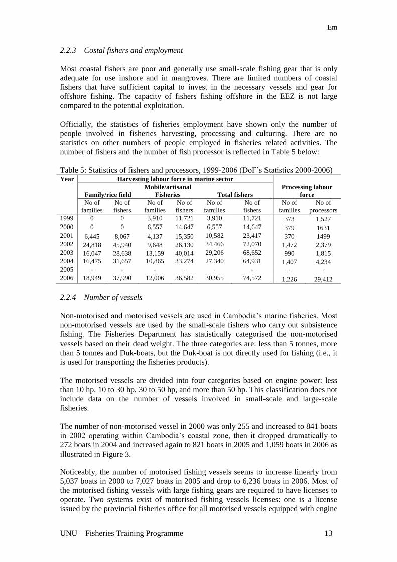
Em
UNU ndash Fisheries Training Programme 13
223 Costal fishers and employment
Most coastal fishers are poor and generally use small-scale fishing gear that is only
adequate for use inshore and in mangroves There are limited numbers of coastal
fishers that have sufficient capital to invest in the necessary vessels and gear for
offshore fishing The capacity of fishers fishing offshore in the EEZ is not large
compared to the potential exploitation
Officially the statistics of fisheries employment have shown only the number of
people involved in fisheries harvesting processing and culturing There are no
statistics on other numbers of people employed in fisheries related activities The
number of fishers and the number of fish processor is reflected in Table 5 below
Table 5 Statistics of fishers and processors 1999-2006 (DoF‟s Statistics 2000-2006) Year Harvesting labour force in marine sector
Processing labour
force Familyrice field
Mobileartisanal
Fisheries Total fishers
No of
families
No of
fishers
No of
families
No of
fishers
No of
families
No of
fishers
No of
families
No of
processors
1999 0 0 3910 11721 3910 11721 373 1527
2000 0 0 6557 14647 6557 14647 379 1631
2001 6445 8067 4137 15350 10582 23417 370 1499
2002 24818 45940 9648 26130 34466 72070 1472 2379
2003 16047 28638 13159 40014 29206 68652 990 1815
2004 16475 31657 10865 33274 27340 64931 1407 4234
2005 - - - - - - - -
2006 18949 37990 12006 36582 30955 74572 1226 29412
224 Number of vessels
Non-motorised and motorised vessels are used in Cambodia‟s marine fisheries Most
non-motorised vessels are used by the small-scale fishers who carry out subsistence
fishing The Fisheries Department has statistically categorised the non-motorised
vessels based on their dead weight The three categories are less than 5 tonnes more
than 5 tonnes and Duk-boats but the Duk-boat is not directly used for fishing (ie it
is used for transporting the fisheries products)
The motorised vessels are divided into four categories based on engine power less
than 10 hp 10 to 30 hp 30 to 50 hp and more than 50 hp This classification does not
include data on the number of vessels involved in small-scale and large-scale
fisheries
The number of non-motorised vessel in 2000 was only 255 and increased to 841 boats
in 2002 operating within Cambodia‟s coastal zone then it dropped dramatically to
272 boats in 2004 and increased again to 821 boats in 2005 and 1059 boats in 2006 as
illustrated in Figure 3
Noticeably the number of motorised fishing vessels seems to increase linearly from
5037 boats in 2000 to 7027 boats in 2005 and drop to 6236 boats in 2006 Most of
the motorised fishing vessels with large fishing gears are required to have licenses to
operate Two systems exist of motorised fishing vessels licenses one is a license
issued by the provincial fisheries office for all motorised vessels equipped with engine
Em
UNU ndash Fisheries Training Programme 14
power under 33 horse power (hp) and another is a license issued by the Fisheries
Administration for all motorised vessels equipped with an engine power above 33
horse power (hp)
Referring to regulations on offshore and inshore vessels it can be assumed that all the
motorised vessels which have small engine power (below 50 hp) and non-motorised
vessels operate inshore Motorised vessels equipped with engine power greater than
50 hp should operate offshore
Fishing vessels equipped with engine power higher than 50 hp may use a labour force
from 5 to 15 people depending on the fishing gear used For boats with an engine
power higher than 100 hp the labour force may be 15 to 30
Figure 3 Number of marine fishing vessel from 2000-2006 (FiA 2007)
225 Annual contribution of marine fisheries to the economy
According to a government report the marine capture fishery has increased from
36000 tonnes in 2000 to 60500 tonnes in 2006 (Table 2) Thus the average marine
capture fishery was around of 50700 tonnes per year from 2000 to 2006 Try et al
(2006) mentioned that the average market price of marine fish is US$ 1 per kg The
marine capture fishery can be estimated to value US$ 507 million a year at the
market site If the tourism industry in Cambodia shows a steady increase of 20
yearly (MoT 2007) the demand for food consumption for tourists will increase This
leads to an increase in the domestic market price of marine fish in Cambodia and the
marine capture fisheries in 2006 can be estimated to value in total revenue around
US$ 635 million According to Try et al (2006) the capture marine fishery values
account of US$ 15 million to US$ 30 million excluding the illegal export which is
un-reported This estimation was at the average market price of trashfish at 500
Cambodian Riels per kg The share of fisheries in the GDP or government revenue
was 108 in 2000 and the estimate for 2005 is 930 (Table 1)
226 Fisheries landing ports
Landing locations are not separated from fishing locations and harbour facilities are
limited Much of the catch is transferred to Thai vessels at sea for landing in Thailand
(FAO 2005) Landing sites of four main coastal areas are used for statistics a total of
about 131 locations landings exist in Sihanoukvill 69 Koh Kong 55 Kampot 4 and
Em
UNU ndash Fisheries Training Programme 15
Kep City 3 Most landing ports are small and rural services and facilities are poor It
may be concluded that fishery landing ports of four main coastal provinces are not of
interest to the private sector to invest in rather these are subsidised by the
government
23 Mackerel fisheries
Mackerel consists of commercial pelagic groups which include short mackerel Indian
mackerel Indo-Pacific mackerel Spanish mackerel and island mackerel They are the
most important pelagic species in the Gulf of Thailand harvested by commercial and
traditional gears The local name ldquoPlathu Kamongrdquo is used loosely to refer to all
these fish species
231 Mackerel production
The highest recorded annual landing of mackerel (Rastrelliger) was 139220 tonnes
and contributing 14 to all the marine fish landed in 1968 in the whole Gulf of
Thailand Second to this 122156 tonnes or 11 of the marine fisheries landings were
recorded in 1969 (Sea Around Us 2005) These species supported the purse seine and
gillnet fisheries since the early 1960s and have remained important until now In fact
mackerel is the most dominant commercial food fish in the Gulf of Thailand
The catch of mackerel declined from about 40000 tonnes in the 1950s to around 20000
tonnes in the 1980s An unusually sharp increase in catch occurred though in 1965-1971
when the catch reached 140000 tonnes The pressure from the industry in Thailand has
resulted in overexploitation Ahmed et al (2007) state that ldquofor a number of decades
fisheries development in the Gulf of Thailand has concentrated on increasing fishing
effort to maintain or increase the production volumerdquo Most important pelagic fish in
the Gulf of Thailand are fully exploited especially Indo-Pacific mackerel anchovies
round scad and sardines and demersal resource stocks are over-fished (FAO 1995)
Figure 4 Volume of mackerel caught in the Gulf of Thailand from 1950-2004 (Sea
Around Us 2005)
232 Mackerel fisheries exploitation and its catch effort in Cambodia
Mackerel is not only sold on the domestic market but is also exported to Thailand
every year both fresh and processed Mackerel in Cambodia is caught by artisanal
fishermen as well as the industrial fishery The artisanal fishery operates from small
Em
UNU ndash Fisheries Training Programme 16
boats with outboard engines of less than 33 hp Most of these fishing boats use
gillnets to catch in inshore areas The industrial mackerel fishery is operates offshore
using purse seines or driftnets with boat engines up to 50 hp The commercial fishing
boat can stay at sea fishing 2 to 5 days This type of boat has facilities to keep fish for
long time
Since 1990 the catch of mackerel by Cambodia had increased from about 1000
tonnes to 4650 tonnes in 2006 (Table 6) From 2002 to the present the catch has been
stable at around 4500 tonnes but the effort has increased with a corresponding
reduction in CPUE
The gillnet boats fish for mackerel approximately 25 days a month 8 months a year
The purse seine operates only during the dry season period of 5 months (20 days per
month) The purse seine boats have crews of about of 15 to 30 people The gillnet
boats can on the other hand operate with a labour force of only 2 to 3 people
Table 6 Volume caught fishing effort and CPUE of mackerel from 1990-2006 (FiA
2007)
Year
Catches
volume
(tonnes)
Fishing effort CPUE
(Kgperson
day)
Boat used gillnet Boat used purse seine Total
boat
Total
labour Boat Labour
(person) Boat
Labour
(person)
1990 1395 - - - - - - -
1991 1212 - - - - - - -
1992 1101 3 9 13 260 16 269 40
1993 1424 9 27 14 280 23 307 43
1994 1513 31 93 15 300 46 393 31
1995 1683 10 30 16 320 26 350 44
1996 1452 14 42 6 320 30 362 36
1997 1278 114 342 15 300 129 642 13
1998 1447 122 366 15 300 137 666 14
1999 1738 172 516 8 160 180 676 15
2000 1559 155 465 10 200 165 665 14
2001 1731 56 168 10 200 66 368 32
2002 4300 50 150 10 200 60 350 86
2003 4421 73 219 13 260 86 479 63
2004 4764 117 351 10 200 127 551 53
2005 4906 250 750 4 80 254 830 31
2006 4650 181 543 6 120 187 663 39
233 Mackerel fish processing products
The mackerel in Cambodia is traditionally processes by salted or steaming For
steamed fish ldquoshort body mackerelrdquo is the local name called as Trey Chom Houy but
for salting ldquoSpanish mackerelrdquo is used the local name is Trey Borb Most production
is for the domestic market Data is limited on export
234 Marketing and price of mackerels
Locally the price of mackerel and its products can be different between markets
throughout the land However the difference between the markets of the four
Cambodian coastal areas is small The Sihanoukville market site is the main
Em
UNU ndash Fisheries Training Programme 17
distribution centre of marine fisheries products into the local market thus the market
price of Mackerel fishes and its products in Sihanoukvill can be assumed as the local
market standard price of Mackerel fishes and its products According to monthly
reports of the Marine Fishery Division the price of mackerel at the landing site and
domestic market is actually increasing especially in the wet season when catch is
small and but demand is high
In 2006 the price of short mackerel at the landing site from January to September
fluctuated from US$ 450 to US$ 625 per tonne1 (Figure 5) Based on data estimated
by the Fishery Administration the landing volume of mackerel species in 2006 was
about 4650 tonnes and can be estimated at around US$ 252 million or 4 of the
marine fishery revenue in 2006 Spanish mackerel is selling at a high price at the
landing and market site but the landing volume is small compared to short mackerel
The landing price of Spanish mackerel within a 9 month period in the year 2006
fluctuated increasingly from US$ 1375 to US$ 3500 per tonne Figure 5 illustrates
the price of short mackerel and Spanish mackerel correlated at two sites domestic
market and local landing site
In general the price of marine fish at landing as well as market site has increased over
the years due to an increase in the fishing operational cost Moreover increased
population leads to high market demand for human consumption whereas the natural
resources are gradually decreasing Thuok et al (2001) stated that marketing channels for
marine products are not so well developed for food security and economy reasons it is
believed that emphasis should be placed by the administration in support of the private sector
on the development and enhancement of marketing of marine fishery products
Figure 5 Price of mackerels at landing and market site for 9 months in 2006 (FiA
2007)
1 The price of mackerel at landing site was conducted and reported to the Fishery Administration by Marine
Fishery Division from January to September in 2006
Em
UNU ndash Fisheries Training Programme 18
24 Marine fisheries resources management in Cambodia
241 Law and regulation
The Cambodian marine fishery is managed under the Fisheries Law of 2006 which is
an improved and updated version of the law from 1987 The main objective of the law
and regulation is to manage and conserve the marine fishery resources in a sustainable
manner Additional objectives are to generate governmental revenue improve the
livelihood of local communities and achieve ecologically sound management by an
improved statistical system gear restrictions area limitations and time closures
Management objectives other than those in the Fishery Law 2006 exist and are
attained by the Ministry of Agriculture Forestry and Fishery (proclaim issue) ie
closed season from 15 January to 31 March for mackerel species
For management purposes the marine fisheries are divided into two groups
Coastal fisheries small family-scale fishing operating in fishing zone 1 which
extends from the coast to a depth of 20 m this fishing zone was almost managed by
community fisheries The coastal community fisheries were established after the
government recognised the poor management of the fisheries sector which resulted in
a movement for reform in 2000 Nowadays 40 community fisheries have been
established along the coast to encourage coastal dwellers to participate in the
management of their resources Fishers use boats without engines or with engines of
less than 50 hp Licenses are not required for boats with no engine or with engines
below 33 hp but for boats with more than 33 hp engines a license fee of 27000 Riels
(US$ 7) per horsepower per year is required Fishing activities are not allowed to
include other fishing gears such as trawls or light fishing
Commercial fisheries refer to large-scale fishing from 20 m depths to the limits of the
EEZ Boats used have engines with more than 50 hp which must be licensed for a fee
of 27000 Riels (US$ 7) per horsepower per year Prohibited fishing gears and
methods include pair trawling light fishing and other illegal fishing gears All marine
fisheries are open year round apart from mackerel for which fishing is banned from
15 January to 31 March (DoF 2001d) Most of the small boats (engine lt 50 hp)
marine fishing fleets use alternative multi-fishing practices following the seasonal
appearance of marine resources including purse-seines gill nets push nets and
trawling Foreign poachers use prohibited gears such as large bottom trawls long drift
nets pair trawlers light fishing and explosives (DoF 2001d)
242 Management and administration
Despite a few limitations on the fisheries in the Gulf of Thailand fisheries there fall
under the framework of unregulated open access In addition there are no limits
placed on the amount of gears that can be used the amount of time that can be spent
fishing or on the quantity of fish that may be captured
Generally coastal fishers can operate all year round by using many different types of
fishing gears However the use of fishing gears is dependent on a number of critical
factors including (1) the capital invested (2) experience and traditions of the fishing
communities in different locations along the coast (3) seasonal abundance of different
Em
UNU ndash Fisheries Training Programme 19
species (4) seasonal weather conditions and (5) ecological conditions associated with
the fishing grounds (eg inshore offshore mangrove coral reef etc)
Fishing in offshore areas is still a challenge and there is a lack of strong law
enforcement measures against illegal fishing from neighbouring countries It is a
problem represented in the low annual production of marine fisheries The present
management of data collection is not sufficient to develop plans for scientific
management of marine fish stocks The lack of knowledge of fish biology ecology
and their dynamics results in a poor understanding of the recent changes in marine
fish stocks (MAFF-DoF 2004)
On the other hand the fisheries competency is still inadequate This is true in terms of
inspection specialists and the lack of adequate physical means to enforce legislation
such as protection against illegal fishing (ie the Fisheries Administration is less able
to set up or install the right technology a high speed boat radio communication and
other facilities for coast guard operations) Furthermore in the 1990s the political
environment was unstable which affected the business environment and led to less
investment capital
However the government and Fisheries Administration have overcome many
obstacles to develop and manage marine fisheries resources as well as the fisheries
sector in the past years Especially a recent achievement is the Fishery Law
completely promulgated public using in 2006 (FiA 2007) The new law was updated
from the previous Fishery Law of 1987 which was based on legislation from 1956
1958 and 1960 (revised) The updated law was also drafted with participation from
stakeholders IOs NGOs and relevant partners through research study and sustainable
development projects on the fisheries sector framework In terms of gains marine
production through fishing effort as well as improve capacity of fishing and biomass
management in EEZ
3 THE PRINCIPLES OF FISHERIES MANAGEMENT
This chapter has been adapted from the lecture notes in the UNU-FTP specialist
course on Fisheries Policy and Planning by Prof Ragnar Arnanon
The need for fisheries management stems fundamentally from the fact that fish
resources are common property It is well known both from theory and experience
that common property resources will be overexploited and possibly irreversibly
depleted unless subjected to appropriate fisheries management Essentially the
fisheries management regime is a set of social prescriptions and procedures that
control the fishing activity Similarly fisheries management requires either collective
action at the industry level or external usually government intervention
The principles of fisheries management or fisheries management regimes consist of i)
the fisheries management system (FMS) ii) monitoring control and surveillance
(MCS) and iii) fisheries judicial system (FJS) These three components of the
fisheries management regime are strongly interdependent All three components of the
fisheries management regime are crucial to its success They are links in the same
chain If one of them fails the fisheries management regime as a whole fails
Em
UNU ndash Fisheries Training Programme 20
31 The fisheries management system (FMS)
The fisheries management system specifies the regulatory framework for the fishing
activity It consists of all the rules that the fishing activity must obey such as gear and
area restrictions fishing licences catch quotas etc In many countries most fisheries
rules are based on explicit legislation In others they are primarily based on social
customs and conventions
The fisheries management system is basically a set of rules about how the fishery
should be conducted These rules may be formal ndash for instance in the form of
published laws and regulations ndash or they may be informal ndash a part of the social culture
governing fishing behaviour In most fisheries both types of fisheries management
rules the formal and the informal apply The purpose of the fisheries management
system is to contribute to the generation of net economic benefits flowing from the
fishery
The fisheries management represents the application of specific fisheries management
instruments or tools Typical fisheries management tools are for instance fishing gear
restrictions limitations on the number of allowable fishing days during the year area
closures and so on Thus the fisheries management tools are like variables or more
precisely control variables and the fisheries management measures the values that can
be chosen for these control variables
Now fisheries management systems consist of particular combinations of one or more
of these tools Thus obviously the number of possible fisheries management systems
increases very fast with the number of available fisheries management systems Most
of them may however be grouped into two broad classes i) Direct fisheries
management and ii) indirect fisheries management as illustrated in Figure 6
Figure 6 Fisheries management systems a classification (adapted from lecture notes
UNU-FTP 2007 introduced by professor Arnason)
Direct fisheries management attempts to control the components of the fishing
activity directly by commands or more often restrictions that must be adhered to
Indirect economic fisheries management by contrast attempts to induce the fishing
firms to behave differently by modifying the operating conditions of the fishery
without imposing direct constraints The difference between direct biological and
economic fisheries management lies in what they seek to control Direct biological
fisheries management attempts to alter the biological yield of the fishery Thus under
biological fisheries management for instance the sustainable yield curve is normally
shifted Direct economic fisheries management attempts to alter the behaviour of the
Em
UNU ndash Fisheries Training Programme 21
fishing firm days vessel size etc Thus direct economic management generally
affects the cost structure of the fishery directly
Indirect fisheries management alters the operating conditions of the fishing industry
There are of course many ways to do this Most however belong to two main
categories (a) taxes (and subsidies) which basically alter the prices facing the fishing
industry and (b) property rights which alter the nature of the external effects imposed
by the fishing firm on one another
Most fisheries management tools are fall quite naturally into one of the fisheries
management categories in Figure 6 The main exception is the total harvesting
restriction or total allowable catch (TAC) Of all the fisheries management systems
considered above only (i) certain property right arrangements and (ii) tax on catch
seem to be theoretically capable of delivering the full potential economic benefits of
fisheries Direct fisheries management irrespective of whether it is based on
biological or economic restrictions seems particularly inept for this purpose
Em
UNU ndash Fisheries Training Programme 22
32 Monitoring control and surveillance (MCS)
The primary task of the monitoring control and surveillance system is to observe the
fishing industry‟s activities and to enforce its adherence to the rules of the fisheries
management system Its secondary but nevertheless very important task is to collect
data about the fishery that can be used to improve both the fisheries management and
fisheries judicial system as well as the monitoring control and surveillance system
itself Broadly speaking the phrase refers to two activities i) the monitoring of the
fishery and the activities of the fishing (harvesting) industry and ii) the enforcement
of fisheries management rules
MCS is as already discussed a crucial component of any fisheries management
regime Logically it is the management authority that must conduct and co-ordinate
the MCS activity although it may engage contractors it is the central fisheries
manager ie the government that operates the MCS activity
The monitoring part of MCS involves collection of the relevant biological data about
the fish stocks and the surrounding ecosystem as well as the relevant technical
economic and behavioural data about the fishing industry and its activities The
monitoring activity is conducted for essentially two purposes i) to gather information
for improving the fisheries management ie data generation monitoring and ii) to
gather information for the purpose of enforcing existing fisheries management rules
ie enforcement monitoring It is important to realise that in order to transform
fisheries data into sensible decisions on fisheries management measures and
modifications of the fisheries management system a good deal of biological and
economic research has to take place Hence is should be clear that research both
biological and economic is an integral part of the monitoring part of the MCS
activity
The enforcement part of MCS consists of acting upon alleged violations of fisheries
management rules It generally takes place where and when the violating activity
occurs The action taken may be of several degrees of severity i) induce the violator
end the illegal activity ii) impose a penalty ie an administrative penalty typically a
fine or a temporary revoking of fishing licence iii) indict the alleged violator and iv)
apprehend and indict the alleged violator In this case the alleged violator is
apprehended (a penalty in itself) and also formally charged for the offence
It should be clear that if the fishing firms are profit maximisers enforcement action
will in general not suffice to generate sufficient adherence to the fisheries
management rules unless the level of monitoring and enforcement is extremely
highly relative to the fishing activity Since the former implies that a decentralised
fishery can never be efficient and the latter is obviously far too expensive compared to
the value of the fishery we may conclude that any reasonable MCS system must rely
on (ii)-(iv) to a significant extent For later reference it is useful to note that the
enforcement part of MCS especially degrees (iii) and (iv) above is linked to the
operations of the fisheries judicial system and in fact depends on it if it is to be
effective
The cost of MCS in fisheries is by no means negligible The available indications
(Arnason et al 2002) suggest that this cost usually ranges between 2 and 10 of
Em
UNU ndash Fisheries Training Programme 23
the total landed value of national the fisheries According to Arnason et al (2002) the
most important MCS cost items appear to be i) enforcement at sea and on land ii)
data collection and research and iii) policy formulation and system administration
Enforcement costs especially those at sea are generally very high and as a whole
usually account for well over half of the total MCS costs Data collection and research
costs typically account for over a third of the total MCS costs with the most costly
item being biological research The rest of MCS costs are accounted for by policy
formulation and general administration costs
33 Fisheries judicial system (FJS)
The fisheries judicial system is part of the general judicial system It should be noted
however that in most societies the formal judicial system is to process alleged
violations of fisheries management rules and issue sanctions to those deemed to have
violated the rules The fisheries judicial system thus complements the monitoring
control and surveillance activities in enforcing the fisheries management rules
The purpose of the fisheries judicial system (FJS) is to i) process alleged violations of
fisheries rules and ii) apply sanctions as appropriate It follows that the FJS must
contain well defined procedures as to how to process alleged violations What are the
courts how may cases be referred to the courts what are the appeal procedures time
limits and so on Without the support of the fisheries judicial system the MCS
activity would not work Alleged violators would simply go to court and get off with
penalties insufficient to deter them from their illegal activities Hence the MCS
activity would be of little use In particular it would not succeed in enforcing the
fisheries rules
It is often found that the fisheries judicial system is the weakest link in the fisheries
management regime The public information and awareness of the judicial system is
not well distributed and the people then are not well-informed Fundamentally the
judiciary system is fairly independent of the executive and legislative branches of
government As a result the fisheries management regime is much less amenable to
reform and change than the other two components The trials and judgements are
passed according to law custom and convention The judicial system in executing
laws and judgements generally has little understanding of the intricacies of the FMR
This suggests the need to include carefully designed laws concerning the treatment of
fisheries violations the burden of proof penalties etc in the fisheries legislation
defining the fisheries management regime
The main objective of the FJS is to endorse the enforcement part of the MCS activity
In particular the FJS determines crucial components of the probability that a violator
of fisheries legislation will suffer penalties The adherence to fisheries management
rules requires sufficiently high administrative costs in processing these allegations
Generally any expected cost of violations can be generated by the appropriate
combination of enforcement and penalties To find this appropriate combination it is
necessary to obtain an empirical estimation from the increased enforcement activity
and improved FJS and its implications to the expected costs of violations
Em
UNU ndash Fisheries Training Programme 24
4 MODELLING
The bio-economic model applied in this chapter has been adapted from the lecture
notes in the UNU-FTP specialist course on Fisheries Policy and Planning by Prof
Ragnar Arnanon
The model applied in this report is used to explain the mackerel fishery in Cambodia
and investigate improvements in its utilisation it is a simple bio-economic model of
the fishery resources The model chosen is based on the work of Gordon (1954) and
Schaefer (1957) (Anderson G L 1981) who developed a basic bio-economic model
for fisheries management The main elements of this model are i) a biomass growth
function which represents the biology of the model ii) a harvest function which
constitutes the link between the biological and economic part of the model and iii) a
fisheries profit function which represents the economic part Particularly for
prediction of the maximum sustainable yield (MSY) of the mackerel fishery we apply
the ldquosurplus production modelsrdquo a simple model introduced by Graham (1935)
(Anderson G L 1981) but they are often referred to as ldquoSchaefer modelsrdquo This
approach was selected for the following reasons i) the Cambodian mackerel fishery
data is very limited and thus does not support an advanced bio-economic model ii)
the model developed here can later be extended and refined when more and better
data becomes available More precisely the model is as follow
x = G(x) ndash y (Biomass growth function) (1)
where x represents biomass x is biomass growth and y is harvest The function G(x) is
natural biomass growth
y = Y(ex) (Harvesting function) (2)
The volume of harvest is taken to depend positively on fishing effort as well as the
size of the biomass to which the fishing is applied
π = p∙Y(ex) ndash C(e) (Profit function) (3)
Where p represents the price of fish landing and C(e) is the cost function of fishing
effort The profit function depends on the fish price the sustainable fish yield and the
fishing operation costs The fishing costs depend on the use of economic inputs
which is the fishing effort can represent the profit function equation
The above model comprises three elementary functions the natural growth function
G(x) the harvesting function Y(ex) and the cost function C(e) It adopts the widely
used specific form for these functions
41 The biomass growth function
Populations of organisms cannot grow infinitely the growth of organisms is
constrained by environmental conditions and food availability It has been shown that
populations of organisms strive to stabilise at the highest possible population size for
a given set of conditions (Schaefer 1954) (Anderson G L 1981) Marginal growth of
a population increases when the size of the population decreases and marginal growth
Em
UNU ndash Fisheries Training Programme 25
decreases when the size of the population increases this may be called density
dependent growth Biological growth of such populations may be expressed as
follows
G(x) = rx ndash sx2 (4)
Where x is population size r is the growth rate of the population and s is the mortality
rate which is negative This is the parabolic equation also referred to as Verhults‟
equation or the logistic growth equation (Schaefer 1954) (Anderson G L 1981)
When the population reaches the environmental carrying capacity (K) growth and
mortality of the population is equal and rate of change of population size with respect
to time (dxdt) becomes zero The mortality rate s can now be expressed in terms of r
and K as
(5)
From equation (5) substitute s in equation (4) we get the most commonly used
expression of the logistic growth equation and equation (4) can be rewriten as
(6)
Fox (1970) (Arnason R 2007) outlined an alternative surplus yield model assuming
the Gompertz growth function resulting in an exponential relationship between
fishing effort and population size and an asymmetrical harvest curve (Fox 1970)
(Arnason R 2007) The generalised form of the Gompertz curve can be represented
as (Winsor 1932) (Arnason R and Bjorndal T 1991)
F(x) = micro∙x(lnK ndash lnx) (7)
In this formulation the carrying capacity of the biomass is K as in the logistic
formulation However unlike the logistic the Fox-Gompertz growth function is not
symmetric and the intrinsic growth rate is infinite compared to r for the
logistic
The major difference between the logistic model and the Fox model is that at lower
population sizes the Fox model predicts a higher growth rate than the logistic model
At higher population sizes the logistic model predicts a higher growth rate than the
prediction by the Fox model In the logistic model maximum growth occurs at half of
the maximum population level In the Fox model maximum growth occurs at a
population level of less than the half of the maximum population around 37 of the
maximum population On the other hand the population growth curve of the Fox
model is skewed to the left while the population growth curve of logistic model is
symmetrical
Em
UNU ndash Fisheries Training Programme 26
Figure 7 Illustrates the logistic biomass growth model G(x)
Figure 8 Illustrates the Fox biomass growth model G(x)
For biomass growth we consider the logistic and the Fox
G(x) = α∙x - β∙x2
(8)
F(x) = α∙x - β∙ln(x)∙x (9)
42 The harvesting function
Assuming that each unit of effort harvest equals the amount from the targeted stock
and an equilibrium situation where catch equals natural growth the equilibrium stock
size (x) may be expressed in terms of carrying capacity (K) catchability coefficient
(q) and fishing effort (e) For the harvesting model in accordance to the generalised
Schaefer (1954) (Anderson G L 1981) version
Y(ex) = q∙e∙xb (10)
Where the coefficient b indicates the degree of schooling behaviour by the fish which
b Є[01]
43 The cost function
Consequently the costs of fishing effort will be a linear function of the amount of
effort ndash index of economic input in the form of labour investment fuel maintenance
and supplies fixed costs and overhead that is devoted to the fishery on an annual
basis The annual cost of fishing C(e) is proportional to effort (e) For this report it
was assumed that the fishing boats are homogeneous The cost function is expressed
as
Em
UNU ndash Fisheries Training Programme 27
C(e) = c∙e + fk (11)
Where c represents marginal costs and fk represents fixed costs
44 The complete model
The complete model based under those function specifications becomes
Biomass growth function
- = α∙x - β∙x2 ndash y (Logistic) (12)
- = α∙x - β∙ln(x)∙x ndash y (Fox 1970) (13)
Harvesting function
- y = q∙e∙xb (14)
Profit function
- π = p∙y ndash c∙e + fk (15)
The last two equations can be combined to yield a simpler version of the model
- π = p∙y ndash(cq)∙y∙x-b
+ fk (16)
The ratio (cq) is viewed as a single parameter known as the normalised marginal cost
It is shown that the marginal cost and catchability c and q are not displayed in an
independent role in this model What counts in the model is the ratio of the two
constant parameters
45 Sustainable yield
The annual rate of renewal of fish stock depends on three major factors biological
environment physical environment and magnitude of the remaining population
Biological and physical environment may be considered to be constant in the long run
(Schaefer 1954) (Anderson G L 1981) Population size is reduced by natural and
fishing mortality Harvesting increases the total mortality As the fish population
strives to balance the total mortality with growth the population reaches a new
equilibrium at a point where the growth rate equals total mortality which occurs at a
lower population size than the environmental carrying capacity level K When the fish
stock reaches equilibrium with a given effort level all biological growth of the
population is harvested and there is no need for change in the population size
y(ex) = G(x) (17)
(18)
and when
Em
UNU ndash Fisheries Training Programme 28
(19)
by substituting x in the equation (18) with equation (19) we get the long term catch
equation
(20)
This implies that although harvest is a function of effort and stock size for the short
term in the long run stock size becomes only a function of effort (given that
environmental conditions are constant) and the sustainable yield too becomes a
function of effort only
Equation (8) takes the form of a parabolic equation which allows us to use linear
regression in order to estimate the parameters of the function of sustainable harvest
(y) Dividing both sides of equation (8) by effort (e) we get the linear equation of
catch per unit effort (CPUE)
(21)
Assuming that biological growth of the subjected population follows the model
suggested by Gowpertz and also assuming the fleet is homogenous and all vessels
have the same fishing power
(22)
by substituting x in equation (6) with (22) the equation became as below
(23)
Dividing both sides of equation (23) by fishing effort (e) yields
(24)
A long-linear expression is found by
(25)
46 Maximum sustainable yield (MSY)
The objective of the application of the ldquosurplus production modelsrdquo is to determine
the optimum level of effort that is the effort that produces the maximum yield that can
be sustained without affecting the long-term productivity of the stock the so-called
maximum sustainable yield (MSY) Because holistic models are much simpler than
analytical models the data requirements are also less demanding There is for
example no need to determine cohorts and therefore no need for age determination
Em
UNU ndash Fisheries Training Programme 29
This is one of the main reasons for the relative popularity of surplus production
models in tropical fish stock assessment Surplus production models can be applied
when data are available on the yield (by species) and of the effort expended over a
certain number of years The fishing effort must have undergone substantial changes
over the period covered The basic models were expressed as follows
461 Surplus production models
The maximum sustainable yield (MSY) can be estimated from the following input
data
- f(i) = effort in year i where i = 1 2 3 hellip n
- Y(i) = yield in year i where i = 1 2 3 hellip n
- Yf = yield (catch in weight) per unit of effort in year t
Yf may be derived form the yield Y(i) of year i for the entire fishery and the
corresponding effort f(i) by
(i) Yf = Y(i) f(i) where i = 1 2 3 hellip n (26)
The simplest way of expressing yield per unit of effort Yf as a function of the effort
f is the linear model suggested by Schaefer (1954) (Anderson G L 1981)
(ii) Y(i) f(i) = a + b f(i) if f(i) le -ab (27)
The intercept ldquoardquo is the Yf value obtained just after the first boat fishes on the stock
for the first time The intercept therefore must be positive The slope ldquobrdquo must be
negative if the catch per unit of effort Yf decreases for increasing effort f Thus -ab
is positive and Yf is zero for ldquofrdquo = -ab (Sparre P and Venema C S 1998) The
equation (27) is a statistically estimable version of equation of equation (21) Schaefer
model
An alternative model was introduced by Fox (1970) (Arnason R 2007) It gives a
curved line when Yf is plotted directly on effort ldquofrdquo but a straight line when the
logarithms of Yf are plotted on effort
(iii) Ln(Y(i) f(i)) = c + d f(i) where ldquocrdquo is ldquoardquo and ldquodrdquo is ldquobrdquo (28)
Equation (28) is called the ldquoFox modelrdquo which can also be written
(iv) Y(i) f(i) = exp(c + d f(i)) (29)
Equation (29) is a statistically estimable version of equation (25) Fox model
Both models conform to the assumption that Yf declines as effort increases but they
differ in the sense that the Schaefer model implies one effort level for which Yf
equals zero namely when f = -ab whereas in the Fox model Yf is greater than zero
for all values of ldquofrdquo
Em
UNU ndash Fisheries Training Programme 30
However to obtain an estimate of the maximum sustainable yield (MSY) and to
determine at which level of effort MSY may be rewritten equations (27) and (29)
expressing the yield as a function of effort by multiplying both sides of the equation
by f(i)
Schaefer
(v) Y(t) = a f(i) + b f(i)2 if f(i) lt -ab (30)
Or Y(i) = 0 if f(i) = -ab
(vi) Y(i) = f(i) exp(c + d f(i)) (31)
From equation (30) the Schaefer model is a parabola which has its maximum value
of Y(i) the MSY level at an effort level
(vii) (32)
and the corresponding yield
(viii) (33)
From equation (31) the Fox model is an asymmetric curve with a maximum
sustainable yield level with a fairly steep slope on the left side and a much more
gradual decline on the right of the maximum The YMSY and fMSY for the Fox model
can be calculated by formulas which are derived from equation (31) by differentiating
Y with respect to ldquofrdquo and solve dYdf = 0 for ldquofrdquo
(ix) (34)
(x) (35)
The estimation procedures for the parameters (Schaefer a amp b Fox c amp d) will be
explained on the basis of the data given in Table 7 Since we are dealing with a
straight line in the case of the Schaefer model and a curve which has been linearised
by taking the logarithm in case of the Fox model the determination of a b and c d
requires two linear regressions of f(i) on Y(i)f(i) and f(i) on ln(Y(i)f(i)) respectively The
results of the two regressions are presented in Table 7 including a maximum
sustainable yield and its correspondent optimum level of effort Thus are determined
the relationships between catch per unit of effort and effort for both models
462 Biomass dynamic models
The formulation of the Schaefer surplus production model in its continuous and
discrete form the logistic model to include catch we obtain
(xi) Bt+1 = Bt + rB ndash B2 ndash Ct (36)
Where r is the intrinsic rate of increase K the carrying capacity Bt the abundance
(biomass) and Ct is the catch at time t It is common practice to assume that catch is
proportional to fishing effort and stock size (Hilborn and Walters 1992 Haddon
2001) In the Schaefer model the biomass level that sustains the maximum
Em
UNU ndash Fisheries Training Programme 31
sustainable yield denoted by Bmsy is at one half of K Maximum sustainable yield is
defined as
(xii) (37)
And the effort that sustains the maximum sustainable yield is
(xiii) (38)
where q is the catchability coefficient also called a nuisance or scaling parameter
One major assumption in the use of the surplus production model is that the
catchability coefficient remains constant over time (Haddon 2001)
463 Specifying priors
The quality of data and lack of prior results forces me to consider alternative methods
of measuring growth rate (r) To overcome this limitation r was estimated using the
equation proposed by Sullivan (1991) (Pauly D 1983) for non-gadoid species In this
formulation r is a function of the von Bertalanffy growth coefficient (k) asymptotic
(Winfin) weight fish so growth rate function can be expressed r = 0947 + 1189k ndash
0095 ln(Winfin) which asymptotic (Winfin) equation is Winfin (Linfin) where
(Pauly‟s formula)
Where and are the coefficient of the length-weight relationship for Rastrelliger
species Linfin is asymptotic length Lmax (cm) is maximum length of mackerel fish
mackerel asymptotic weight (Winfin) was calculated with available parameter estimates
= 3213 Lmax = 35 cm and k = 06-16 (data is available at the website
Fishbaseorg) In this report k is assumed 1 for mackerel fisheries in Cambodian
coastal waters as well as the whole of the Gulf of Thailand
5 ESTIMATION OF MODEL
51 Data sources
The data for this report was collected from different sources The data required was
classified into two categories biological and fisheries data The Fisheries
Administration (FiA) previously called the Department of Fisheries (DoF) is the
main institution responsibly for the fisheries sector of Cambodia Therefore most of
the data used in this report is derived from the Fisheries Administration‟s data sources
and they were considered to be the prime sources for this study
Most of the data of the FiA are only available from 1990 to 2006 ie total landed of
marine fisheries production statistics of fishing boats gears (fishing effort) However
the data on catches by species or group is very poor for the past three decades Since
2000 the data collection in this category was made more systematic
The Fisheries Administration of Cambodia provides economic input data such as total
cost of fishing effort (cost of boat ndash engine fuel consumption and labour costs)
landing price of the mackerel fishery in base year 2006 fixed costs and overheads
Em
UNU ndash Fisheries Training Programme 32
Therefore this data is based on quick interviewing or communications between
fishery officers and the fishing ground costal guards and also from fishing
experimentalists
Whereas the biological data such as the fish stock status virgin stock biomass (Xmax)
maximum sustainable yield (MSY) fish abundance density distribution and
mackerel schooling parameter (b) are not available for mackerel in Cambodia or the
Gulf of Thailand In terms of projects for regional research study for mackerel species
in the Gulf of Thailand it seems that previous research has not yet been taken into
account Even though some projects were carried out in parts of Thailand waters this
seems to be representative of the Gulf it‟s limited biological data and specifying
analysis of mackerel species
Most are only focused on multi-species or demersal species ie Theory and
management of tropical multi-species stocks (Pauly D 1983) Development of
fisheries in the Gulf of Thailand Large Marine Ecosystem Analysis of an unplanned
experiment Overfishing in the Gulf of Thailand Policy challenges and bioeconomic
analysis (Ahmed et al 2007) Status of demersal fishery resources in the Gulf of
Thailand Potential yield of marine fishery resources in Southeast Asia etc
However the articles named above are considered as the basis of assumable
knowledge in this report such as schooling parameters biomass stock of mackerel
catchability coefficient in order to predict or estimate MSY virgin biomass stock of
mackerel for Cambodia as well as the general status of this species in the Gulf of
Thailand
Moreover for estimating the growth rate (r) of mackerel the report subscribed to data
which was relevant for maximum length (Lmax) growth coefficient (k) and length-
weight relationship ) of Rastrelliger species in the Gulf of Thailand which was
available at FAO or the Fishbaseorg website
Some data had to be derived through calculation of the available ones so as to meet
the needs of this research study Data that had never been collected nor documented
but available from fishery officers fishing ground guardians and fishermen was
communicated both by means telephone and e-mail
The bio-economic model of fisheries is specified above containing six unknown
parameters there are α β c q b and fk but c and q can be performed as a normalised
marginal cost (cq) formatting In addition to calculating profits and rents of fisheries
exploitation information on landed volume (y) fishing effort (e) and biomass (x) is
required Suppose that optimal equilibrium harvest and biomass will be determined
by the optimality conditions so only the six unknown parameters need to be known in
order to calculate rents It is reflected if the position of profits is zero the position of
rents in this model (linear in y) will be simply the parameter fk and pieces of
information to calculate rents would be take in account or calculated There are many
ways to estimate the unknowns in the fisheries model defined by equations (12) (13)
and (16) The following details based on a number of available data on fisheries
which are included
- Biological data which are available could be guessed
- Fisheries data for a specific year are available and could be guessed
Em
UNU ndash Fisheries Training Programme 33
Based on available data it is straight forward to calculate the unknowns of equations
(12) (13) and (16) as listed below
Table showing the formulas used to determine the unknown using the data available Formula to calculate the parameters of models
Unknowns Formula
Logistic function
Α
Β
Biomass in base year x(t)
Fox function
Α
Β
Biomass in base year x(t)
Normalise marginal cost
Fixed cost fk
The schooling parameter b b
Landing in base year t y(t) y(t)
Price of landing in base year t p(t) p(t)
Formula to calculate the MSY and fMSY by the surplus production model
Schaefer
MSY
fMSY
Fox
MSY
fMSY
Intercept Schaefer (a) Fox (c)
Slope Schaefer (b) Fox (d)
Formula to calculate the carrying capacity (K) and catchability coefficient (q) by the biomass
dynamic model
Carrying capacity (K)
Catchability coefficient (q)
Growth rate (r) r = 0947+1189kndash0095ln(Winfin)
Asymptotic weight (Winfin) Winfin (Linfin)
Asymptotic length (Linfin) (Paulyrsquos formula)
Growth coefficient k
Length-weight relationship
Maximum length (cm) Lmax
The data suggested are as follows
Em
UNU ndash Fisheries Training Programme 34
Table showing biological and fisheries data necessary for estimating model‟s
unknown values 1- Biological data
Maximum sustainable yield MSY
Virgin stock biomass Xmax
The schooling parameter b
Maximum length Lmax
Length-weight relationship
2- Fisheries data in a base year
Biomass growth in year t (t)
Landing in base year t y(t)
Price of landing in year t p(t)
Fishing effort t e(t)
Profit in base year t π(t)
Fixed cost ratio in base year t (fkTC(t) ε(t)
These are pieces of information However it is worth noting that there are many other
ways to obtain the estimates of the model‟s unknowns based on different sets of data
52 Parameter estimation
521 Maximum sustainable yield (MSY)
Information on the biomass and sustainable yield of fisheries is among the most
crucial required for the management of fisheries resources In Cambodia the actual
mackerel fish biomass is not known However based on landed data time series and
fishing effort of mackerel from 1992 ndash 2006 we can estimate the maximum
sustainable yield and optimum level of effort by using surplus production models
Graham (1935) (Pauly D 1983) Cambodia has been a small actor in the mackerel
fisheries in the Gulf of Thailand in recent decades Only during recent years has it
been increasing its catches and improving its management of the resource It is
therefore necessary to check for model stability to verify if the relationship between
effort and catch has remained stable over the period of the data I apply the CUSUM
test for structural stability since no obvious structural break point is available to test
explicitly The CUSUM test results for the Schaefer and Fox models for the whole
period 1992 to 2006 are presented in Figures 9 and 10
-10
-8
-6
-4
-2
0
2
4
6
8
10
2 4 6 8 10 12 14
Observation
CUSUM plot with 95 confidence band
Figure 9 CUSUM plot of Schaefer model Figure 10 CUSUM plot of Fox model
-10
-5
0
5
10
15
2 4 6 8 10 12 14
Observation
CUSUM plot with 95 confidence band
Em
UNU ndash Fisheries Training Programme 35
The CUSUM test results clearly indicate that a structural change occurred during the
period According to the test the most likely breakpoint is 2001 In order to estimate a
model with a separate YMSY and fMSY for the two periods now identified before and
after the break we introduce a dummy variable for the period 2002-2006 and an
interaction between the dummy variable and the effort (f) The results for the different
slope and intercepts are reported in Table 8
The estimation was carried out in the statistical package GRETL The full output is
available in Appendices 2 and 3 The hypothesis that one model can sufficiently
explain the relationship between CPUE and effort during the whole period was tested
and clearly rejected for both the Schaefer and the Fox models at 1 level of
significance in favour of the alternative hypothesis that a structural break occurred in
2001
The results from estimations during the period 2002-2006 are Schaefer model
(intercept 007739 slope -0000255) and Fox model (intercept -2356298 slope
0006642) These figures are used to determine the optimum level of effort and
maximum sustainable yield according to the equation shown in Table 7
Table 7 The calculation procedure for estimating the MSY and fMSY by the Schaefer
model and by the Fox model using catch and effort data from 1992-2006 of the EEZ
of Cambodia
Year
(i)
Yield
(yi)
(1000 tonnes)
Effort (fi)
(boat)
(x)
Schaefer Fox
Yifi
(y)
Yifi
(y)
1992 1101 16 0068 -2690
1993 1424 23 0063 -2761
1994 1513 46 0033 -3422
1995 1683 26 0064 -2756
1996 1452 30 0049 -3012
1997 1278 129 0010 -4615
1998 1447 137 0011 -4552
1999 1738 180 0010 -4642
2000 1559 165 0009 -4662
2001 1731 66 0026 -3645
2002 4300 60 0072 -2636
2003 4421 86 0052 -2963
2004 4764 127 0037 -3284
2005 4906 254 0019 -3947
2006 4650 187 0025 -3694
Mean value 1021751 00365 -35521
Standard deviation (sx amp sy) 727333 00231 07702
1- Results of calculates intercept and slope
Whole period (1992-2006)
Intercept (a or c) 0059014636 -2762864933
Slope (b or d) -0000228367 -0007727171
Period 1992-2001
Intercept (a or c) 0063230899 -0605339532
Slope (b or d) -0000353678 -0013085091
Period 2002-2006
Intercept (a or c) 0077391095 -2356298149
Slope (b or d) -000025484 -000664217
2- Calculation MSY and fMSY based on surplus production models
Maximum sustainable yield (MSY)
Em
UNU ndash Fisheries Training Programme 36
Optimum level of fishing effort (fMSY)
Whole period (1992-2006)
YMSY 3813 3005
fMSY 129 129
Period 1992-2001
YMSY 2826 2077
fMSY 89 76
Period 2002-2006
YMSY 5876 5249
fMSY 152 151
The results for the period 2002-2006 of MSY estimate 5876 (Schaefer) 5249 (Fox)
and fMSY equal to 152 (Schaefer) and 151 (Fox) Since the dependent variable is not
the same for the two models it is not possible to test statistically the superiority of one
model over the other (Sparre P and Venema C S 1998) However careful
examination of the data and the suggested models lead to the conclusion that the
Schaefer model is more reasonable for the current situation Its MSY equals 5876
tonnes and effort 152 boats This figure was applied to estimate carrying capacity (K)
or virgin stock biomass (Xmax) and other parameters in the report
522 Virgin stock biomass (Xmax)
The information about virgin stock biomass of mackerel in the Gulf of Thailand as
well as in parts of Cambodia is not known To determine carrying capacity (K) or
virgin biomass stock (Xmax) and catchability coefficient (q) the report study uses the
biomass dynamic models of the Schaefer surplus production models Based on the
results for MSY and corresponding effort reported in Table 8 the value of MSY is
equal to 5873 tonnes and fMSY is equal to 153 boats Based on these estimates the
parameters K can be estimated by the follow equations
Growth parameters of the Sullivan (1991) (Pauly D 1983) equation
where = 3213
where Lmax = 35 cm (Pauly‟s formula)
Table 8 Estimates of r and K at different levels of assumptions of growth coefficient (k) of Rastrelliger brachysoma in the Gulf of Thailand
Categories
of data
YMSY Lmax Linfin Winfin
5876 35 00061 3213 368 6576
k k k K k k
06 08 100 12 14 16
Parameters
r 104398 128178 151958 175738 199518 223298
K 22514 18337 15467 13374 11780 10526
Em
UNU ndash Fisheries Training Programme 37
Assuming that the MSY is 5876 fMSY is 152 and growth coefficient (k) is 1 the result
of estimated basis parameters for r and K is 151958 and 15467 respectively
Therefore the value of carrying capacity (K) or virgin biomass stock (Xmax) estimated
(Table 9) is 15467 tonnes
523 The schooling parameter (b)
Mackerel is the prey it swims fast is known to gather in medium schools and travel
great distances The mackerel fish can be found in estuarine habitats with slightly
reduced salinities and in areas where surface temperature ranges between 20 and
30C Their migratory and schooling nature forming schools of equally sized
individuals The species which aggregate together have a small schooling parameter lt
1 On the basis of this argument the schooling parameter of mackerel fish could be
between 05 to 075 Therefore for the purpose of this study the value of mackerel
schooling parameter was assumed to be 065 This needs to be subjected to sensitivity
analysis to evaluate its effect on the economic benefit of the fisheries
524 Alpha and beta parameter (α)
This parameter was calculated by using the formula below and we considered that the
value of virgin biomass stock and the MSY are known so the alpha and beta was
calculated as follows
Xmax = 15467 (1000 tonnes)
MSY = 5876 (1000 tonnes)
α = 15196
Xmax = 15467 (1000 tonnes)
MSY = 5876 (1000 tonnes)
β = 00983
525 Landings in base year t y(t)
According to the annual fishery report 2006 of the Fisheries Administration it was
estimated that the total landings of marine fisheries in the year 2006 were
approximately 60500 tonnes Particularly the volume landed of mackerel in year
2006 was 4650 tonnes This was the figure adapted for this study
526 Price of landings in base year t p(t)
The price of marine fish in every year is based on the price at Sihanoukville market
site which is the main distribution in the local and export market According to the
monthly report of the Marine Fishery Division the landing price of mackerel in base
year 2006 in the period January to September fluctuated from US$ 450 to US$ 625
per tonne For the purposes of this study this figure is calculated as the average price
of the 9 months at US$ 542 per tonne
Em
UNU ndash Fisheries Training Programme 38
527 Fixed cost ratio in base year eps(t)
For the purposes of this report this figure was calculated depending on the fixed cost
and fishing total cost First the fixed cost was calculated at the rate 3 of total
landing revenue of mackerel The total fishing cost can be see in Appendix 1 of the
cost calculation procedure
Fixed cost (fk) = 3 of landing revenue in base year t
= 3 x US$ 2520300 = US$ 75609
Calculation of the fixed cost ratio as follow
eps (t) or ε(t) = fixed cost total fishing cost
= 756091438203 = 0053 or 53
So eps (t) or ε(t) is 53
528 Fishing effort in base year
Based on the annual fishery report 2006 of the Fisheries Administration the total of
marine motorised fishing boats is 6326 boats The number of fishing boats registered
for fishing mackerel was a total of 187 boats which included 181 fishing boats using
gillnets and six boats using purse seines For this report we standardised them so that
all the boats would be homogenous Therefore we assumed the six boats using purse
seines to be boats using gillnets The figure was assumed with the original gillnet
boat so to come up with the figure 187 gillnet boats This was the value adopted in
this study as the fishing effort
529 Profit in base year (π)
The profit of the base year is the result of subtracting the total fishing cost from the
total landing revenue The total landing revenue and total fishing cost were calculated
as follow
Profit (π) = Revenue (R) ndash Total cost (TC)
- Revenue
Revenue (R) = Landing in base year x Price landing in base year
Revenue (R) = 4650 tonnes x US$ 542 = US$ 2520300
- Total cost
Table 9 shows the total cost as a summary of different costs namely fuel labour food
maintenance license depreciation fixed cost and overhead cost These items were
calculated as follow
Em
UNU ndash Fisheries Training Programme 39
Table 9 Cost of fishery economic inputs
Items Cost (US$)
Fuel and lubricating oil 289850
Labour 636548
Food 130900
Maintenance 98175
Licenses 2805
Depreciation value 88488
Fixed cost 75609
Overhead cost 115828
Total cost (TC) 1438203
- Profit (π) = 2520300 ndash 1438203
π = US$ 1082097
53 Assumption and estimation
Table 10 The assumed mackerel fishery biological and fisheries parameters necessary
for calculating the unknown estimates 1- Biological data Symbol Assumed value
Maximum sustainable yield
(tonnes)
MSY 5876
Virgin stock biomass (tonnes) Xmax 15467
The schooling parameter b 065
2- Fisheries data in base year
Biomass growth in base year
(tonnes)
(t) 4200
Landing in base year (tonnes) y(t) 4650
Price of landing in base
(US$tonne)
p(t) 542
Fishing effort (boat) e(t) 187
Profit in base year (US$) π(t) 1082097
Fixed cost ratio in base year eps(t) or ε(t) 0053
3- Estimated value (calculated)
Logistic function
Alpha α 15196
Beta β 00983
Biomass in base year (tonnes) x(t) 4200
Normalised marginal cost
0745
Fox function
Alpha α 2828
Beta β 1033
Biomass in base year (tonnes) x(t) 9700
Normalised marginal cost
1286
Fixed cost (US$) fk 76000
Price of landing in base year (US$) p(t) 0542
Em
UNU ndash Fisheries Training Programme 40
54 Empirical results
The results of the two models derived from the Arnason modelling approach
programme using Microsoft Office Excel Macro are given in Table 11 The table
shows the estimated results of biomass harvest effort profits and rents at current and
optimal level These results are very useful to outline the effects of different marine
fisheries policies in order to manage the resource It also shows the trend as the results
of operation of mackerel fishery in Cambodian waters in the past years Based on the
Schaefer model the level of current mackerel biomass growth is 4200 tonnes in terms
of optimal biomass level was estimated probably at 8800 tonnes while according to
the Fox results the current biomass growth level is 9700 tonnes stock available and
optimal biomass level is slightly higher (9000 tonnes)
Harvest effort and profits were estimated at optimal level According to Schaefer the
optimal level of harvesting is 5800 tonnes with effort correspondence of about 143
boats and profit around US$ 2 million The Fox model gave an estimated level of
harvest that was lower (5000 tonnes) and a higher effort level (213 boats)
Both models indicate optimal biomass and profits as higher than the current fishing
status of the mackerel fishery However the effort level indicated by the Schaefer is
lower than the current effort level The reason for this is of course that a bigger stock
is less expensive to harvest since catch per unit effort is much higher than at the
current stock size It would therefore be optimal to reduce effort in the short run to
allow the stock to reach an optimal size This would mean that the government should
limit effort eg by implementing a scheme for compensating fishermen for stopping
fishing One such suggestion is depreciation allowances
Economic rent or opportunity cost was also estimated from these two models which
is the cost involved in not engaging in one‟s most profitable alternative activity For
natural resources ie if a high value and low cost fishery will be heavily exploited
and possibly overexploited Conversely a low value and high cost fishery will be
lightly exploited or even unexploited However fishermen will enter or leave a given
fishery after comparing their expected net revenues with income opportunities
elsewhere These common sense predictions are a useful feature of the Gordon model
The results for estimating the rent level are given in Table 11 for the Schaefer and Fox
models The results indicate that the fishermen are unlikely to leave fishing and look
for income opportunities elsewhere As long as positive profits are maintained it is
likely that more and more fishers will enter the fishery unless other more profitable
opportunities are available to them This will ultimately lead to overexploitation
Similarly Christy and Scott (1965) (Flaaten O 1988) state that ldquoBionomic
equilibrium of the unregulated open-access fishery is thus characterised by the
complete dissipation of economic rent Assuming that thing could be otherwise this
dissipated rent constitutes a loss of wealth to society at largerdquo (Clark 2006)
Therefore fishery management must be taken seriously by local communities and
central administrations of Government and enforced by both levels of government
Em
UNU ndash Fisheries Training Programme 41
Table 11 Main results from estimations of the mackerel fisheries
Categories Units Current Optimal Difference
Logistic Fox Logistic Fox Logistic Fox
Biomass 1000mt 42 97 88 90 46 -07
Harvest 1000mt 47 47 58 50 11 04
Effort boat 187 187 143 213 00 00
Profits mUS$ 1082 1082 2004 1099 0920 0017
Rents mUS$ 1158 1158 2080 1176 0922 0017
55 Model simulation and results
The estimates in Table 11 were calculated on the basis of the rent definitions by
Arnason (Arnason R 2007) The calculations were based on the Arnason modelling
approach programme using Microsoft Office Excel Macro the same approach used in
an on-going World Bank Programme in determining the world fisheries rent
It‟s simplicity and robustness in generating output based on limited or scanty data
made it the modelling approach of choice in this study The programme is convenient
to use and to apply to data The outputs are reports on profits rents fishing capacity
and resources biomass on any base year in logistic and Fox distributions Thus the
results in Table 11 are derived from the Arnason modelling approach programme
which was run by Microsoft Office Excel Marco
Iso-profitable curves the curves in Figures 11 and 12 illustrate the summary
description of the mackerel fishery The figure was drawn in the space of biomass and
landings and applies at each point of time and therefore in equilibrium The
parabolic graph illustrates the biomass growth function The biomass function covers
biomass from zero to the carrying capacity of about 15467 tonnes and a maximum
sustainable yield at a level of 5876 tonnes The iso-profit curves are in harvest units
(multiples of MSY) For the purposes of this fishery the harvest units are in thousand
tonnes The equation for an iso-profit curve is
Where gam = 00 when Iso-profits = 0
gam = 025 when Iso-profits = 025MSY
gam = 050 when Iso-profits = 050MSY
In order to convert this into monetary units the harvest units should be multiplied by
the landing price as follows
Profit (π) = p∙y where p is the landing price and y is landing volume
Em
UNU ndash Fisheries Training Programme 42
Figure 11 The fishery in biomass-yield (biomass growth harvest) space for the
logistic distribution
Figure 12 The fishery in biomass-yield (biomass growth harvest) space for the Fox
distribution
For any biomass level if catches lie within this curve then a biological equilibrium
prevails The other curves in this diagram are variable iso-profit curves (eg location
of biomass and harvests which presents constant variable profits measured in
mackerel volume units The highest sustainable profits are obtained where an iso-
profit curve is a tangent to the biomass growth function As the two diagrams suggest
this occurs at a biomass of some 8800 tonnes for logistic and Fox at a level of 9000
tonnes to quarantine harvest at about 5800 tonnes (logistic) and 5000 tonnes
Therefore at this point the profits and rent from the mackerel fishery from the two
models is US$ 11 million to US$ 21 million per year
Current
harvesting status
Current
harvesting status
Sustainable
harvests curve
Sustainable
harvests curve
Em
UNU ndash Fisheries Training Programme 43
6 OPTIMUM SUSTAINABLE YIELD AND FISHERIES ECONOMICS
The concept of optimum sustainable yield (OSY) or more simply optimum yield
(OY) has become increasingly common both in theory and as the basis of actual
management schemes The OSY is generally defined as MSY modified by relevant
economic social environmental and other factors The term of MSY often underpins
the practical definition of OSY Furthermore although the term OSY may give the
impression of being some long-run goal to be attained and maintained on a continuing
basis in fact the optimum yield may have to be less than sustainable in some years
and more in others if full use is to be made of a stock (Cunningham et al 1985)
Therefore the greater the environmental fluctuations the greater the difference should
be between biological optimum sustainable yield and MSY
61 Maximum sustainable yield of mackerel fishery and current catches
The concept of maximum sustainable yield (MSY) defined by Punt and Smith (2001)
(FAO 2001) as the largest annual catch or yield that may be taken from a stock
continuously without affecting the catch in future years has had a fluctuating history
of favour and scorn in fisheries management (King 2007) This concept adapted from
the original MSY concept in the 1930s and mathematical models that related yield to
fishing mortality began to appear in the 1950s Therefore Schaefer (1954 1957)
(Anderson G L 1981) constructed the first model that is most associated with MSY
which is the surplus production model
Figure 13 illustrates MSY derived from the two models and actual volume catches of
mackerel It can be seen that the two models give slightly different results According
to Schaefer the MSY level is 5876 tonnes at an effort level fMSY of 152 boats while
according to the Fox model the MSY level is a little bit lower (5249 tonnes) and at an
effort level fMSY of 151 boats According to both models the effort level surpassed
fMSY in 2005 (254 boats) and the yield was below MSY
The maximum sustainable yield occurs when the fish population growth rate reaches a
maximum It is the maximum that can be caught on a sustainable level without
reducing the long-term stock and it is obtained by exerting that level of effort at
which total sustainable revenue is maximised (Van den Bergh et al 2006) An
equilibrium point to the right of the MSY is inefficient in terms of the bio-economic
model Based on results from the Schaefer and Fox models it is possible for
Cambodian fishers to increase catches of mackerel to a maximum level between about
5249 and 5876 tonnes per year However fishing effort should be reduced from 187
boats (current) to a level of effort correspondent to around 150 boats
Em
UNU ndash Fisheries Training Programme 44
Figure 13 Maximum sustainable yield and actual catches
62 Maximum economic yield
This section presents a discussion of economic output based on the results derived
from the Arnason modelling approach It uses MSY and virgin biomass stock
estimated using alternative modelling of the surplus production and biomass dynamic
models as input Therefore effort corresponding to an optimum level may be
different to the optimum level of effort that was estimated using the surplus
production model However the two results are a useful basis to compare effort
between MSY and OSY or MEY The optimal biomass harvest profits and rents are
not available from the surplus production and biomass dynamic models The summary
of main results from the modelling approach programmed is given in Table 11
Economic variables are often included in the biological Schaefer model to model the
relationship between sustainable revenue fishing costs and fishing effort (King 1995)
The relationship between revenue fishing costs and fishing effort is used to show how
a fishery with no limits on the number of participating fishers (an open-access fishery)
will become overexploited in the economic as well as the biological sense (King
2007)
The fishing cost line cuts the yield (revenue) curve at the break even (open access)
point where revenue balances fishing cost Maximum economic yield is reached
where the distance between the revenue curve and the cost line is the greatest The
effort that maximises economic yields fMEY is generally different from MSY effort
The level is determined by the development of unit effort cost as stock size increases
The relationship between revenue fishing costs and fishing effort of mackerel fished
in Cambodia is illustrated in Figures 14 and 15 According to the Schaefer curve
(Figure 14) the maximum economic yield (MEY) of mackerel at a total profit equal
to US$ 2 million that the total revenue is probably US$ 315 million with an optimum
biomass level of 8800 tonnes to guarantee a harvest of 5800 tonnes (Table 11) The
corresponding effective effort level is about 143 standard boats Building up the stock
would increase catch per unit effort and reduce the harvesting cost The optimum
would be to employ only 143 vessels where each vessel catches more and at a lower
cost per unit catch The optimal harvest and effort levels are lower than the level of
MSY 5876
MSY 5249
fMSY
Em
UNU ndash Fisheries Training Programme 45
MSY (5876 tonnes) and effort (152 boats) from the Surplus production model
According to the theory of economic yield MSY is always higher than OSY and its
corresponding effort Focusing on economic yield rather than maximising catch
guarantees that the fisheries contribute a maximum amount of rents into Cambodian
society to aid development
Figure 14 Schaefer curve of relationship between revenue costs and effort
The results from the Fox model (Figure 15) indicate that the fishing cost line cuts the
revenue curve at a break even point where that revenue just balances fishing costs at
around US$ 3 million with corresponding fishing effort (fOA) at a level of around 420
boats This is the ldquoopen-accessrdquo solution with no revenues In an open-access fishery
effort is expected to move to equilibrium where the economic forces affecting
fishermen and the biological productivity of the resources are in balance (Van Den
Bergh et al 2006) However the Fox curve illustrates the maximum economic yield
(US$ 1099 million) at the optimum effort level at a 213 boats corresponding with a
yield (catch) of around 5000 tonnes (Table 11) It is very important that the fisheries
resources in Cambodia are well managed because improved management has the
potential to create new jobs and improve the economic situation for the population of
coastal areas
The optimum effort given by this solution is much higher than Schaefer‟s optimum
effort and is even higher than the current fishing effort (187 boats) This seems quite
odd It seems that the earlier conclusion is true that the Fox model does not describe
the Cambodian mackerel fishery adequately No emphasis will therefore be put on the
results from the Fox model
f0187
MEY
fMEY
0143
Em
UNU ndash Fisheries Training Programme 46
Figure 15 Fox curve of relationship between revenue cost and effort
63 Sensitivity analysis of optimal fisheries policy
The model used to calculate the optimal mackerel policy discussed above is subject to
considerable uncertainty Among other things the parameter estimates used in the
model may well be erroneous To check the robustness of the calculated optimal
policy to parameter misspecification a sensitivity analysis of the optimal policy to
parameter values was conducted More precisely we calculated the optimal profit for
other values of the parameters The results of this exercise are reported in Table 12
and Figures 16 and 17
The sensitivity results on optimal profits (economic rents) of the mackerel fishery
based on changed assumptions of the base year (2006) indicate that the net profits of
mackerel are in the range between US$ 1277 million and US$ 2923 million when the
MSY is assumed to change between -20 and 30 (logistic) According to the Fox
model the profit of mackerel increased from US$ 1166 million to US$ 1241 million
when changing MSY -20 to 30 Similarly the parameter of landing price
increased from -30 to 30 (logistic) profit gain from US$ 166 million to US$
2356 million and Fox model profit gain from US$ 1082 million to US$ 1171
million with the price of landed decreasing from 30 to -30 It was observed that
the optimal profits have slightly changed or no sensitivity on changes made on base
year profit fishing effort and virgin stock status (Table 12)
The sensitivity analysis further indicates that even if the biological parameter
estimations and information on price and costs are incorrect or erroneous the
mackerel fishery has the potential to generate economic rents ranging between US$
1166 million and US$ 2923 million from both models
f0187
Economic
break-
even point
MEY
fMEY fOA
Em
UNU ndash Fisheries Training Programme 47
Table 12 Sensitivity analysis of optimal mackerel fisheries policy
Change
Logistic -30 -20 -10 0 10 20 30
MSY (1000 tonnes) NA 1277 1678 2004 2315 2621 2923
Xmax (1000 tonnes) 2004 2004 2004 2004 2004 2004 2004
Schooling parameter 1842 1899 1953 2004 2053 21 2144
Biomass growth 2268 2184 2097 2004 19 1772 NA
Harvest ( 1000 tonnes) 2591 2394 22 2004 1797 1555 NA
Price (m US$1000 tonnes) 166 1773 1888 2004 2121 2238 2356
Effort (boat) 2004 2004 2004 2004 2004 2004 2004
Initial Profit (m US$) 1755 1837 192 2004 2089 2174 226
Fox
MSY (1000 tonnes) 1166 1082 1099 1138 1187 1241
Virgin stock (1000 tonnes) 1099 1099 1099 1099 1099 1099 1099
Schooling parameter 1135 112 1108 1099 1093 1088 1085
Biomass growth (1000
tonnes) 0914 0967 1028 1099 1187 1307 NA
Harvest (1000 tonnes) 1521 1302 117 1099 1084 114 NA
Price (m US$1000 tonnes) 1171 1137 1115 1099 109 1084 1082
Effort (boat) 1099 1099 1099 1099 1099 1099 1099
Initial Profit (m US$) 0758 0866 098 1099 1224 1355 149
Figure 16 Sensitivity analysis Schaefer chart of mackerel fisheries in Cambodia
Figure 17 Sensitivity analysis Fox chart of mackerel fisheries in Cambodia
Em
UNU ndash Fisheries Training Programme 48
7 DISCUSSION
This study has aimed to provide an overview of the mackerel fisheries in Cambodian
waters The major obstacle has been the lack of good data on catches and effort by
foreign vessels in the Cambodian EEZ and the Gulf off Thailand as a whole
However the biological data of mackerel such as maximum length of fish length-
weight relationship and growth coefficient for the species as whole in the Gulf are
available With better data it would have been possible to address the issues of fair
sharing of resource rents and optimal management of the mackerel stocks of the Gulf
of Thailand as a whole But as mentioned this is beyond the scope of this particular
paper due to data problems The estimates obtained here are however believed to be
fairly realistic in terms of describing the current situation and the possibilities for
improvements in Cambodian management of the mackerel stock if the issues of
foreign catches is not addressed The method employed in this paper can be regarded
as a modification of the extrapolation method with biological and environmental
information of mackerel fisheries aspects
The bio-economic models developed here show that the mackerel fishery is generally
quite profitable It further shows that proper effort management can substantially
increase profits As the estimated results in Table 11 and sensitivity analysis Table 12
clearly show that stock size should be allowed to increase and that optimum stock size
would allow for annual caches of approximately 6000 tonnes per year with economic
rents (profits) of about US$ 2 million under efficient management and good
enforcement
However the results indicate that in order to reach the optimum sustainable yield and
maximise economic yield mackerel fishers needed to reduce fishing effort from 187
boats to about 150 boats These are mostly inshore boats since very few boats have
the capacity to operate offshore To optimise resource utilisation and maximise
economic rents from fisheries in the Gulf of Thailand it would be necessary to
address the issues of management in cooperation between all the nations surrounding
the Gulf The potential rent increases for Cambodia from such cooperation are very
large To stimulate the interest for and development of such cooperation some action
must be taken On one hand to further intensify research of the resources biological
studies and upgrading of catch and effort statistics need to be made on a national basis
and to establish the comparability of these data in the region On the other hand there
is an urgent need for information on the capacity of resources fishing grounds to
model the effects of the improved management measures in the coastal zone (EEZ) as
well as the Gulf
The trans-boundary fish stocks of the Gulf of Thailand are not a unique case Consider
for example the case of the Norwegian spring-spawning herring fishery (Bjorndal et
al 2004) where the cooperation between three nations in managing its fish stock is
very similar to the mackerel stock in the Gulf of Thailand between Thailand Vietnam
Malaysia and Cambodia The dynamic bio-economic model used for the tri-nations in
managing their herring stocks showed that the benefits of international cooperation far
exceed the returns of a competitive open access fishery Therefore this model does
well in forecasting the outcome of competitive open access fisheries showing an
increased and sustained fishing effort by all fleets while harvest levels decline
(Bjorndal et al 2004)
Em
UNU ndash Fisheries Training Programme 49
8 CONCLUSION
This paper estimated the Schaefer and Fox economic models for the mackerel
fisheries in Cambodia The results from the Schaefer and Fox models indicate that the
mackerel fish stocks are both biologically and economically overexploited and there
are opportunities to increase the rents from the mackerel stocks in the EEZ by
reducing effort and allowing the stocks to increase in size The reason for the
overexploitation may lie in the nature of the fishing boats that are most common in
the Cambodian fleet ie small inshore vessels Their small size and limited operation
capacity confines them to inshore areas leading to over-fishing of these areas
According to the results of this study the mackerel fishery could increase its total
allowable catch (TAC) to the maximum level of OSY and maximise the economic
rents by curtailing both the excessive fishing effort and exploitation in the inshore
areas and expand the fishing capacity in the offshore areas Therefore this study
suggests that the marine fisheries sectorFisheries Administration set up a
development scheme to extend these policies to mackerel fishing
Prior to outlining the policy this study should be aware of the national concerns An
optimal resource utilisation based solely on achieving economic efficiency
inadequately addresses the broader social issues In this regard a policy aimed at
maximum sustainable yield should be modified according to the precautionary
principle rather than basing it on the maximum economic yield This has advantages
since it offers to alleviate employment and distributional concerns in the coastal
dwellers In terms of payments the winners and the losers in this fishery may perhaps
be financed by increasing the license fees or limiting access for foreign fishing
vessels
Cooperation with neighbouring countries is very important in order to achieve
efficient management of marine fisheries resources of migratory species in the Gulf of
Thailand Such cooperation should include all the country members in the Gulf area
The mackerel fishery is complex in nature due to the multi-nation exploitation and the
local migratory behaviour of the species moving between several coastal EEZs
especially the overlapping fishing zones in the Gulf Thereby for sustainable
management of the fisheries resources there is a need for regional cooperation with
all the relevant member countries
Although this study is limited to the mackerel fishery in Cambodia the bionomic
model presents the basis for future policy analysis for a regional fisheries
management approach in the Gulf of Thailand
Em
UNU ndash Fisheries Training Programme 50
ACKNOWLEDGMENTS
I would like to express my gratitude to my supervisor Dr Dadi Mar Kristofersson of
the University of Iceland for his excellent technical guidance criticism and comments
during the time of developing and writing this report
I am grateful to Dr Tumi Tomasson Mr Thor Asgeirsson Ms Sigridur Ingvarsdottir
and Mr Gudni Magnus Eiriksson for their hospitality support and guidance during
the six months of study in Iceland I am thankful to the Board of the UNU-FTP and
United Nations University for offering me the opportunity to participate in this course
and funding my studies I would also like to extend my gratitude to the General
Director of the Marine Research Institute and staff for their very good support for
hosting this learning environment
I am thankful to Prof Ragnar Arnason for his support and allowing me to use his
approach programme in this report
Finally I would like to thank the General Director of the Fisheries Administration of
Cambodia for allowing me to participate on this training course
Em
UNU ndash Fisheries Training Programme 51
LIST OF REFERENCES
Ahmed M Boonchuwongse P Drchboon W and Squires D 2007 Overfishing in
the Gulf of Thailand Policy challenges and bioeconomic analysis Environment and
Department Economic 12 145-172 Cambridge University Press [Electronic version]
lthttpjournalscambrideorg article_s1355770X06003433gt
APIP 2001b Marine fisheries review Agriculture Productivity Improvement Project
World Bank
Anderson G L 1981 Economic Analysis for Fisheries Management Plans Ann
Arbor Science Michigan USA
Arnason R 2007 The Principles and Practice of Fisheries Management UNU-
Fisheries Training Programme‟s lecture note
Arnason R Hannesson R and Schrank W E 2002 Cost of Fisheries Management
The Cases of Iceland Norway and Newfoundland Marine Policy 24 233-43
Arnason R and Bjorndal T 1991 Essays on the Economics of Migratory Fish
Stocks Germany Springer-Verlag Berlin Heidelberg
Bjorndal T Dordon V D Kaitala V and Lindroos M 2004 International
Management Strategies for a Straddling Fish Stock A Bio-Economic Simulation
Model of the Norwegian Spring-Spawning Herring Fishery International amp Resource
Economics 29 435-457 2004 Kluwer Academic Publishers Printed in Netherlands
[Electronic version]
lt httpideasrepecorgakapenreecv29y2004i4p435-457htmlgt
CFDO-IMM 2005 Cambodia Post-Harvest Fisheries Overview An output from the
DFID-funded Post-Harvest Fisheries Live livelihood Project Department of
Fisheries Ministry of Agriculture Forestry and Fisheries Phnom Penh Cambodia
Clark C W 2006 The worldwide Crisis in Fisheries Economic Models and Human
Behavior Cambridge University Press Cambridge UK 12-13
Christy FT and Scott AD 1965 The Common Wealth in Ocean Fisheries (Johns
Hopkins University Press Baltimore
Csavas I Doulman D Peter T Prado J and Debas L 1994 Cambodia ndash
Rehabilitation and Development Needs of the Fisheries Sector Fisheries Circular N
873 FAO Rome
Cunningham S Dunn M R and Whitmarsh D 1985 Fisheries Economics an
Introduction Mansell Publishing Limited London England 106
DoF 2001d Marine Fisheries Review Technical Paper no 3 Agriculture Productivity
Improvement Project (APIP) ndash Fisheries Component Department of Fisheries Phnom
Penh 41
Em
UNU ndash Fisheries Training Programme 52
FAO 2005 Review of the State of World Marine Fishery Resources FAO Fisheries
Technical Paper 457 Food and Agriculture Organization of the United Nations
Rome [Electronic version]
lt ftpftpfaoorgdocrepfao007y5852ey5852e00pdfgt
FAO 2001 Report of a Bio-Economic Modelling Workshop and a Policy Dialogue
Meeting on the Thai demersal fisheries in the Gulf of Thailand Food and Agriculture
Organization of the United Nations Rome [Electronic version]
lt httpwwwfaoorgdocrepFIELD006Y1160EY1160E00HTMgt
FAO 1999 Fishery Country Profile ndash the Kingdom of Cambodia FAO Rome
FiA 2007 Annual Report 2006 Status of Cambodia Fisheries Sector Fisheries
Administration Ministry of Agriculture Forestry and Fisheries Phnom Penh
Fishbaseorg Rastrelliger brachysoma in Cambodia (Short mackerel)
lthttpwwwfishbaseorgCountryCountrySpeciesSummarycfmc_code=116ampid=10
9gt
Fishbaseorg Length-Weigh Relationship for Rastrelliger brachysoma (Inner Gulf of
Thailand)
lthttpwwwfishbaseorgPopDynFishLWSummarycfmID=109ampid2=420ampgenusn
ame=Rastrelligerampspeciesname=brachysomaampfc=416ampgm_a=0011979339063ampgm_
b=31294281605gt
Flaaten O 1988 The economics of multispecies harvesting theory and application to
the Barents sea fisheries Germany Springer-Verlag Berlin Heidelberg
Fox 1970 WW Fox An exponential surplus-yield model for optimizing exploited
fish populations Trans Am Fish Soc 99 (1970) pp 80ndash88
Gillett R 2004 The Marine Fisheries of Cambodia Food and Agriculture
Organization of the United Nations Rome 2004 [Electronic version]
lt httpwwwfaoorgdocrep007j1617ej1617e00htmgt
Graham M 1935 Modern theory of exploiting a fishery and application to North
Sea trawling J Edu Conseil Int Explor Mer 10 pp 264ndash274
Gordon HS 1954 The economic theory of a common property resource the fishery
J Pol Econ 82 pp 124ndash142
Haddon M 2001 Modelling and Quantitative Methods in Fisheries Chapman amp
HallCRC (39)
Hilborn R and Walters C J 1992 Quantitative Fisheries Stock Assessment
Chapman amp Hall New York
Em
UNU ndash Fisheries Training Programme 53
King M 1995 Fisheries Biology Assessment and Management Fishing News
Books 206
King M 2007 Fisheries Biology Assessment and Management Blckwell Publishing
239-277
MAFF-DoF 2004 Fisheries Development Action Plan 2005-2008 Ministry of
Agriculture Forestry and Fisheries ndash Department of Fisheries Version 3
MoP 2006 National Strategic Development Plan 2006-2010 Royal Government of
Cambodia Ministry of Planning
MoT 2007 Tourism Statistics Report 2006 Ministry of Tourism of Cambodia Phnom
Penh
NACA 2004 STREAM Support to Regional Aquatic Resources Management
System Requirement Report for bdquoLevel 2‟ ndash National Management Institutions
Fisheries Department in Cambodia
Pauly D 1983 Some Simple Methods for the Assessment of Tropical Fish Stocks
FAO Corporate document repository Italy Rome 1984 [Electronic version]
lt httpwwwfaoorgDOCREP003X6845EX6845E00HTMgt
Schaefer MB 1954 Some aspects of the dynamics of populations important to the
management of commercial marine fisheries IATTC Bull 1 (1954) pp 25ndash56
Schaefer MB 1957 A study of the dynamics of the fishery for yellowfin tuna in the
eastern tropical Pacific Ocean IATTC Bull 2 (1957) pp 245ndash285
Sea Around Us 2005 A Five-Year Retrospective 1999 to 2004 Sea Around Us
project Fisheries Centre of The University of British Columbia [Electronic version]
lthttpwwwseaaroundusorgRetrospectFhtmdate=420May202005amptitle=Sea
20Around20Us20A20Five-Year20Retrospective20199920to202004gt
Sparre P and Venema C S 1998 Introduction to Tropical Fish Stock Assessment
FAO Fisheries Technical Paper 3061 Rev 2 Rome Italy 279-281 [Electronic
version]
lt ftpftpfaoorgdocrepfaow5449ew5449e00pdfgt
Sullivan KJ 1991 The estimation of parameters of the multispecies production
model ICES Mar Sci Symp 193 (1991) pp 185ndash193
Tana T S 1997 Status of marine biodiversity of Cambodia - Phuket Marine
Biological Center Special Publication 17(1) 175-180
Thuok N Nam S and Sereyvath T S 2001 Cambodiarsquos Fish Processing and
Marketing and Distribution of Fish and Fishery Products focusing on Market
Opportunities and Export Potentials Department of Fisheries Phnom Penh
Em
UNU ndash Fisheries Training Programme 54
Try I and Jensense K R 2006 National Report on Stock and Fish Habitat in Key
Cambodia Coastal Zones FiAUNEPGEF Phnom Penh Cambodia
Try I 2003 Fish stock and habitats of regional global and stransboundary
significance in the South China Sea (Cambodia) Reversing environmental
degradation trends in the South China Sea and Gulf of Thailand UNEP and Global
Environment Facility
UNDP 2008 Human Development Report 20072008 Published for the United
Nation Development Programme 231 [Electronic version]
httphdrundporgenmediahdr_20072008_en_completepdf
Van Den Bergh JCJM Hoekstra J Imeso R Nunes PALD and Blaeij AT
2006 Bioeconomic Modelling and Valuation of Exploited Marine Ecosystems
Netherlands Springer 31-32
Winsor C P 1932 ldquoThe Gompertz Curve as a Growth CurverdquoProc Nat Acad
Sci18 1ndash8
Em
UNU ndash Fisheries Training Programme 55
Appendix 1 Cost calculation of marine fishing operating in Cambodia 2006
Unit US$
Categories Boat Cost per boat Total
1- Investment cost 3380 632060
Boat 187 2500 467500
Engine 187 370 69190
Gear box 187 280 52360
Nets 187 125 23375
Shaft 187 75 14025
Propeller 187 30 5610
2- Depreciation value (14 per year of investment capital) 88488
3- Operation cost 6194 1158278
Fuel 187 1350 252450
Lubricating oil 187 200 37400
Food 187 700 130900
Labour cost 187 3404 636548
Boat repairing 187 350 65450
Engine repairing 187 125 23375
Nets repair 187 50 9350
License 187 15 2805
Overhead (10 of operation cost) 115828
Fixed cost (3 of total landing revenue) 75609
Total cost (TC) 1438203
Appendix 2 Use GRETL checking the parameter stability (intercept and slope)
Model 1 OLS estimates using the 15 observations 1992-2006
Dependent variable Schaefer model
VARIABLE COEFFICIENT STDERROR T STAT P-VALUE
const 00613596 000704380 8711 lt000001
e -0000243077 568248E-05 -4278 000090
Mean of dependent variable = 00365333
Standard deviation of dep var = 00231142
Sum of squared residuals = 000310676
Standard error of residuals = 0015459
Unadjusted R-squared = 0584643
Adjusted R-squared = 0552692
Degrees of freedom = 13
Durbin-Watson statistic = 139926
First-order autocorrelation coeff = 0276578
Log-likelihood = 423326
Akaike information criterion (AIC) = -806652
Schwarz Bayesian criterion (BIC) = -792491
Hannan-Quinn criterion (HQC) = -806803
Em
UNU ndash Fisheries Training Programme 56
CUSUM test for parameter stability ndash
Null hypothesis no change in parameters
Test statistic Harvey-Collier t(12) = 273394
with p-value = P(t(12) gt 273394) = 00181338
-10
-8
-6
-4
-2
0
2
4
6
8
10
2 4 6 8 10 12 14
Observation
CUSUM plot with 95 confidence band
Chow test for structural break at observation 2001 -
Null hypothesis no structural break
Test statistic F(2 11) = 442883
with p-value = P(F(2 11) gt 442883) = 00388201
Augmented regression for Chow test
OLS estimates using the 15 observations 1992-2006
Dependent variable sche
VARIABLE COEFFICIENT STDERROR T STAT P-VALUE
const 00653294 000686756 9513 lt000001
e -0000360326 653109E-05 -5517 000018
splitdum -000342892 00127541 -0269 079302
sd_e 0000180322 977605E-05 1845 009218
Mean of dependent variable = 00365333
Standard deviation of dep var = 00231142
Sum of squared residuals = 000172097
Standard error of residuals = 00125081
Unadjusted R-squared = 0769916
Adjusted R-squared = 0707166
F-statistic (3 11) = 122695 (p-value = 0000783)
Durbin-Watson statistic = 26802
First-order autocorrelation coeff = -0366056
Log-likelihood = 467628
Akaike information criterion (AIC) = -855256
Schwarz Bayesian criterion (BIC) = -826934
Hannan-Quinn criterion (HQC) = -855558
Em
UNU ndash Fisheries Training Programme 57
Chow test for structural break at observation 2001
F(2 11) = 4428825 with p-value 0038820
Model 2 OLS estimates using the 15 observations 1992-2006
Dependent variable Schaefer
VARIABLE COEFFICIENT STDERROR T STAT P-VALUE
const 00632309 000531711 11892 lt000001
e -0000353678 521717E-05 -6779 000003
d 00141602 00114717 1234 024279
ed 988389E-05 824769E-05 1198 025595
Mean of dependent variable = 00365333
Standard deviation of dep var = 00231142
Sum of squared residuals = 000110648
Standard error of residuals = 00100294
Unadjusted R-squared = 085207
Adjusted R-squared = 0811725
F-statistic (3 11) = 211198 (p-value = 719e-005)
Durbin-Watson statistic = 265039
First-order autocorrelation coeff = -0392424
Log-likelihood = 500756
Akaike information criterion (AIC) = -921512
Schwarz Bayesian criterion (BIC) = -89319
Hannan-Quinn criterion (HQC) = -921814
Excluding the constant p-value was highest for variable 5 (ed)
Restriction set
1 b[d] = 0
2 b[ed] = 0
Test statistic F(2 11) = 994285 with p-value = 000341974
Restricted estimates
VARIABLE COEFFICIENT STDERROR T STAT P-VALUE
const 00613596 000704380 8711 lt000001
e -0000243077 568248E-05 -4278 000090
d 0000000 0000000 undefined
ed 0000000 0000000 undefined
Standard error of residuals = 0015459
Em
UNU ndash Fisheries Training Programme 58
Model 3 OLS estimates using the 15 observations 1992-2006
Dependent variable Fox
VARIABLE COEFFICIENT STDERROR T STAT P-VALUE
const -276286 0249072 -11093 lt000001
e -000772717 000200935 -3846 000202
Mean of dependent variable = -355207
Standard deviation of dep var = 0770141
Sum of squared residuals = 388459
Standard error of residuals = 0546639
Unadjusted R-squared = 0532183
Adjusted R-squared = 0496197
Degrees of freedom = 13
Durbin-Watson statistic = 0648362
First-order autocorrelation coeff = 0683309
Log-likelihood = -111513
Akaike information criterion (AIC) = 263027
Schwarz Bayesian criterion (BIC) = 277188
Hannan-Quinn criterion (HQC) = 262876
CUSUM test for parameter stability -
Null hypothesis no change in parameters
Test statistic Harvey-Collier t(12) = 318135
with p-value = P(t(12) gt 318135) = 000790142
-10
-5
0
5
10
15
2 4 6 8 10 12 14
Observation
CUSUM plot with 95 confidence band
Chow test for structural break at observation 2001 -
Null hypothesis no structural break
Test statistic F(2 11) = 183004
with p-value = P(F(2 11) gt 183004) = 0000316801
Em
UNU ndash Fisheries Training Programme 59
Augmented regression for Chow test
OLS estimates using the 15 observations 1992-2006
Dependent variable fox
VARIABLE COEFFICIENT STDERROR T STAT P-VALUE
const -257874 0156848 -16441 lt000001
e -00131694 000149163 -8829 lt000001
splitdum -0158563 0291290 -0544 059706
sd_e 000836782 000223275 3748 000322
Mean of dependent variable = -355207
Standard deviation of dep var = 0770141
Sum of squared residuals = 0897686
Standard error of residuals = 0285671
Unadjusted R-squared = 0891893
Adjusted R-squared = 0862409
F-statistic (3 11) = 302502 (p-value = 131e-005)
Durbin-Watson statistic = 246393
First-order autocorrelation coeff = -0240326
Log-likelihood = -0164188
Akaike information criterion (AIC) = 832838
Schwarz Bayesian criterion (BIC) = 111606
Hannan-Quinn criterion (HQC) = 829821
Chow test for structural break at observation 2001
F(2 11) = 18300353 with p-value 0000317
Model 4 OLS estimates using the 15 observations 1992-2006
Dependent variable Fox
VARIABLE COEFFICIENT STDERROR T STAT P-VALUE
const -260534 0104820 -24855 lt000001
e -00130851 000102850 -12722 lt000001
ed 000644292 000162593 3963 000222
d 0249041 0226150 1101 029431
Mean of dependent variable = -355207
Standard deviation of dep var = 0770141
Sum of squared residuals = 0430015
Standard error of residuals = 0197718
Unadjusted R-squared = 0948214
Adjusted R-squared = 093409
F-statistic (3 11) = 671372 (p-value lt 000001)
Durbin-Watson statistic = 229763
First-order autocorrelation coeff = -0181381
Log-likelihood = 535581
Akaike information criterion (AIC) = -271163
Schwarz Bayesian criterion (BIC) = 0120575
Hannan-Quinn criterion (HQC) = -274179
Em
UNU ndash Fisheries Training Programme 60
Excluding the constant p-value was highest for variable 3 (d)
Restriction set
1 b[ed] = 0
2 b[d] = 0
Test statistic F(2 11) = 441849 with p-value = 553047e-006
Restricted estimates
VARIABLE COEFFICIENT STDERROR T STAT P-VALUE
const -276286 0249072 -11093 lt000001
e -000772717 000200935 -3846 000202
ed 0000000 0000000 undefined
d 0000000 0000000 undefined
Standard error of residuals = 0546639
Appendix 3 Summary output of model 1- SUMMARY OUTPUT OF SCHAEFER MODEL
Regression Statistics
Multiple R 092307626
R Square 0852069782
Adjusted R Square 0811725177
Standard Error 0010029405
Observations 15
ANOVA
Regression 3 00063733 000212442 21119795 719144E-05
Residual 11 00011065 000010059
Total 14 00074797
Coefficien
ts Standard
Error t Stat P-value Lower 95
Upper 95
Lower 950
Upper 950
Intercept 00632309 000531711 11892 00000001 0051528 0074934 00515280 00749338
d 00141602 001147168 12344 0242789 -001109 0039409 -0011089 00394092
e -0000354 000005217 -67791 000003 -000047 -000024 -0000469 -0000239
ed 00000988 000008248 11984 025595 -0000083 0000280 -00000827 00002804
SUMMARY OUTPUT
Regression Statistics
Multiple R 07326175
R Square 05367283
Adjusted R
Square 04981224
Standard Error 00157419
Observations 14
Em
UNU ndash Fisheries Training Programme 61
ANOVA 000344518 13902728 0002881089
df SS MS F Significance
F
Regression 1 000344518 000344518 13902728 000288109
Residual 12 000297367 000024781
Total 13 000641886
Coefficient
s
Standard
Error t Stat P-value Lower 95
Upper
95
Lower
950
Upper
950
Intercept 00590146 000785405 75139 00000
07 004190214 0076127 00419021 00761271
16 -0000228 000006125 -37286 00029 -000036181 -000010 -00003618 -00000949
2- SUMMARY OUTPUT OF FOX MODEL
Regression Statistics
Multiple R 072951
R Square 053218
Adjusted R
Square 049620
Standard Error 054664
Observations 15
ANOVA
df SS MS F
Significanc
e F
Regression 1 441906 441906 1478864 000202
Residual 13 388459 029881
Total 14 830365
Coefficien
ts
Standard
Error t Stat P-value Lower 95
Upper
95
Lower
950
Upper
950
Intercept -2762865 024907237 -1109262
0000000
05 -3300953 -2224777 -3300953 -2224777
e -0007727 000200935 -3845599 0002024 -00120681 -0003386 -0012068 -
00033862
SUMMARY OUTPUT
Regression Statistics
Multiple R 0973763
R Square 0948214
Adjusted R Square 0934090
Standard Error 0197718
Observations 15
ANOVA
df SS MS F
Significanc
e F
Regression 3 7873634 2624545 6713717
7 0000000
Residual 11 0430015 0039092
Total 14 8303649
Coefficien
ts
Standard
Error t Stat P-value Lower 95
Upper
95
Lower
950
Upper
950
Intercept -2605340 0104820
-
24855249 0000000 -2836048 -2374631 -2836048 -2374631
Em
UNU ndash Fisheries Training Programme 62
d 0249041 0226150 1101220 0294314 -0248713 0746795 -0248713 0746795
e -0013085 0001029
-
12722470 0000000 -0015349 -0010821 -0015349 -0010821
ed 0006443 0001626 3962599 0002224 0002864 0010022 0002864 0010022
Appendix 4 Summary result from Excel Spreadsheet
Iso-profits
Landings Price Natural biomass growth Iso-profits ( of MSY)
Biom
ass Logistic Fox Logistic Fox 0 25 50 0 25 50
00
NU
M
NU
M 00
NU
M
NU
M
NU
M
NU
M
NU
M
NU
M
NU
M
04 05 05 06 15 -01 -10 -20 00 -05 -09
08 05 05 11 24 -02 -26 -49 -01 -09 -17
12 05 05 16 31 -06 -65 -124 -01 -14 -27
15 05 05 21 37 -41 -465 -889 -02 -20 -39
19 05 05 26 42 13 153 293 -03 -29 -56
23 05 05 30 45 07 78 150 -04 -43 -82
27 05 05 34 49 05 57 110 -06 -66 -127
31 05 05 38 51 04 47 90 -10 -116 -221
35 05 05 41 54 04 41 79 -25 -292 -558
39 05 05 44 55 03 37 72 96 1099 2102
43 05 05 47 57 03 35 66 19 218 417
46 05 05 49 58 03 33 62 11 129 247
50 05 05 52 58 03 31 59 08 95 182
54 05 05 53 59 03 30 57 07 77 148
58 05 05 55 59 03 29 55 06 66 127
62 05 05 56 59 02 28 53 05 59 112
66 05 05 57 58 02 27 52 05 53 102
70 05 05 58 57 02 26 50 04 49 94
73 05 05 59 56 02 26 49 04 46 88
77 05 05 59 55 02 25 48 04 43 83
81 05 05 59 54 02 25 48 04 41 79
85 05 05 58 53 02 24 47 03 39 75
89 05 05 57 51 02 24 46 03 38 72
93 05 05 56 49 02 24 45 03 36 70
97 05 05 55 47 02 23 45 03 35 67
101 05 05 53 45 02 23 44 03 34 65
104 05 05 52 42 02 23 44 03 33 64
108 05 05 49 40 02 23 43 03 32 62
112 05 05 47 37 02 23 43 03 32 61
116 05 05 44 34 02 22 43 03 31 59
120 05 05 41 32 02 22 42 03 31 58
124 05 05 38 29 02 22 42 03 30 57
128 05 05 34 25 02 22 42 03 29 56
131 05 05 30 22 02 22 41 03 29 55
135 05 05 26 19 02 22 41 02 29 55
139 05 05 21 15 02 21 41 02 28 54
143 05 05 16 12 02 21 41 02 28 53
147 05 05 11 08 02 21 40 02 27 53
151 05 05 06 04 02 21 40 02 27 52
155 05 05 00 00 02 21 40 02 27 51
Em
UNU ndash Fisheries Training Programme 63
Appendix 5 Schaefer model estimates the sustainable fishery
Results (The sustainable fishery)
Biomass Biomass growth Harvest Revenues Costs Profits Rents
0 00 00 NUM DIV0 NUM NUM
030934 05 05 02 08 -06 -05
061868 09 09 05 10 -05 -04
092802 13 13 07 11 -04 -03
123736 17 17 09 12 -03 -02
15467 21 21 11 13 -01 00
185604 25 25 13 13 00 01
216538 28 28 15 14 02 03
247472 32 32 17 14 03 04
278406 35 35 19 14 05 06
30934 38 38 20 14 06 07
340274 40 40 22 14 08 08
371208 43 43 23 14 09 10
402142 45 45 25 14 10 11
433076 47 47 26 14 11 12
46401 49 49 27 14 12 13
494944 51 51 28 14 13 14
525878 53 53 29 14 14 15
556812 54 54 29 14 15 16
587746 55 55 30 14 16 17
61868 56 56 31 14 17 18
649614 57 57 31 13 18 18
680548 58 58 31 13 18 19
711482 58 58 32 13 19 20
742416 59 59 32 13 19 20
77335 59 59 32 12 20 20
804284 59 59 32 12 20 21
835218 58 58 32 12 20 21
866152 58 58 31 11 20 21
897086 57 57 31 11 20 21
92802 56 56 31 11 20 21
958954 55 55 30 10 20 21
989888 54 54 29 10 20 20
1020822 53 53 29 09 19 20
1051756 51 51 28 09 19 19
108269 49 49 27 09 18 19
1113624 47 47 26 08 18 18
1144558 45 45 25 08 17 18
1175492 43 43 23 07 16 17
1206426 40 40 22 07 15 16
123736 38 38 20 06 14 15
1268294 35 35 19 06 13 14
1299228 32 32 17 05 12 13
1330162 28 28 15 05 11 11
1361096 25 25 13 04 09 10
139203 21 21 11 04 08 09
1422964 17 17 09 03 06 07
1453898 13 13 07 02 05 05
Em
UNU ndash Fisheries Training Programme 64
1484832 09 09 05 02 03 04
1515766 05 05 02 01 01 02
15467 00 00 00 01 -01 00
Appendix 6 Fox model estimates the sustainable fishery
Results(The sustainable fishery)
Biomass Biomass growth Harvest Revenues Costs Profits Rents
0 NUM NUM NUM NUM NUM NUM
030934 12 12 07 35 -28 -28
061868 21 21 11 37 -26 -25
092802 27 27 15 37 -23 -22
123736 32 32 17 37 -19 -19
15467 37 37 20 36 -16 -16
185604 41 41 22 36 -14 -13
216538 44 44 24 35 -11 -10
247472 47 47 25 34 -09 -08
278406 49 49 27 33 -07 -06
30934 51 51 28 33 -05 -04
340274 53 53 29 32 -03 -02
371208 55 55 30 31 -01 00
402142 56 56 30 30 00 01
433076 57 57 31 29 02 03
46401 58 58 31 28 03 04
494944 58 58 32 27 04 05
525878 59 59 32 26 05 06
556812 59 59 32 26 06 07
587746 59 59 32 25 07 08
61868 59 59 32 24 08 09
649614 58 58 32 23 09 09
680548 58 58 31 22 09 10
711482 57 57 31 21 10 10
742416 56 56 30 20 10 11
77335 55 55 30 20 10 11
804284 54 54 29 19 11 11
835218 53 53 29 18 11 12
866152 52 52 28 17 11 12
897086 50 50 27 16 11 12
92802 49 49 27 16 11 12
958954 47 47 26 15 11 12
989888 46 46 25 14 11 12
1020822 44 44 24 13 11 11
1051756 42 42 23 12 10 11
108269 40 40 22 12 10 11
1113624 38 38 20 11 10 10
1144558 36 36 19 10 09 10
1175492 33 33 18 09 09 09
1206426 31 31 17 09 08 09
123736 29 29 15 08 08 08
1268294 26 26 14 07 07 08
1299228 23 23 13 06 06 07
1330162 21 21 11 06 06 06
1361096 18 18 10 05 05 06
Em
UNU ndash Fisheries Training Programme 65
139203 15 15 08 04 04 05
1422964 12 12 07 04 03 04
1453898 09 09 05 03 02 03
1484832 06 06 03 02 01 02
1515766 03 03 02 01 00 01
15467 00 00 00 01 -01 00
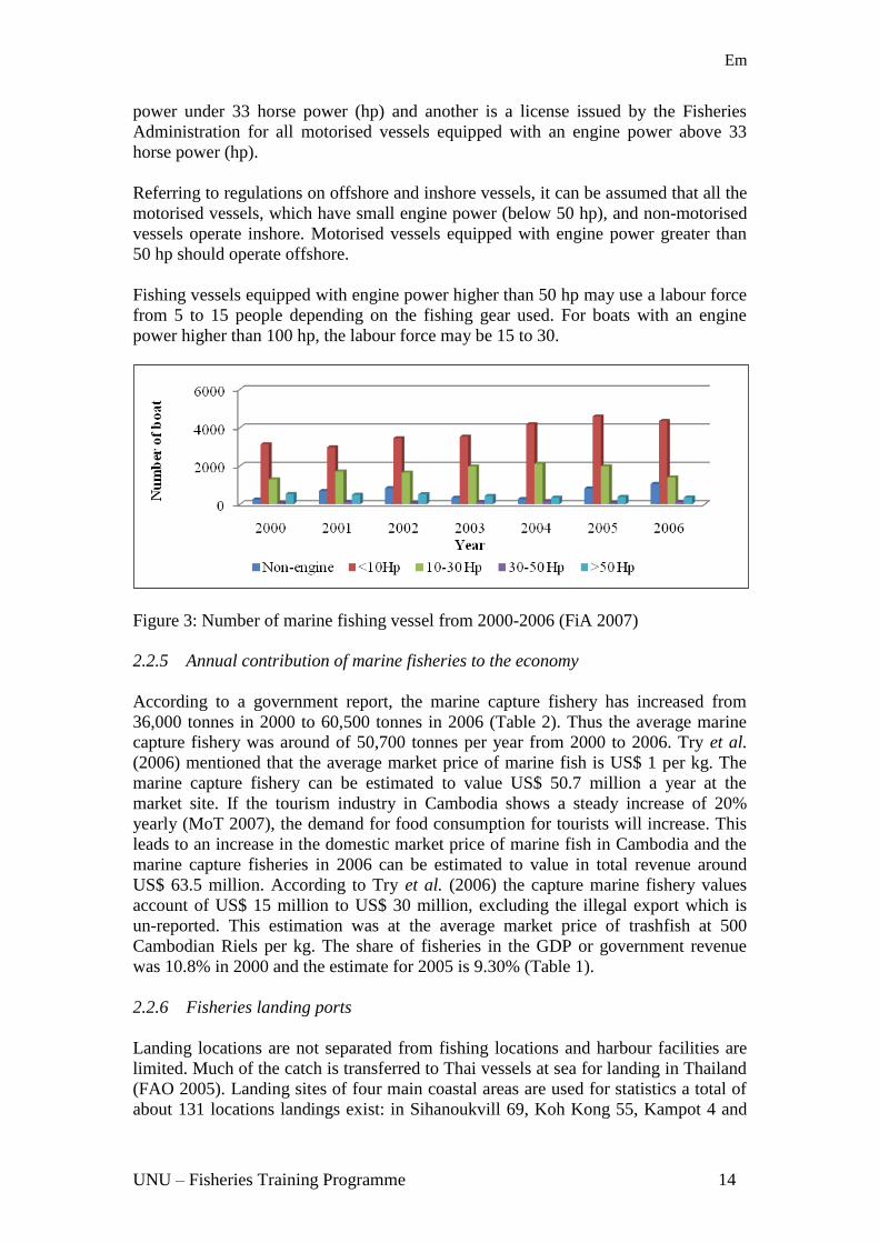
Em
UNU ndash Fisheries Training Programme 14
power under 33 horse power (hp) and another is a license issued by the Fisheries
Administration for all motorised vessels equipped with an engine power above 33
horse power (hp)
Referring to regulations on offshore and inshore vessels it can be assumed that all the
motorised vessels which have small engine power (below 50 hp) and non-motorised
vessels operate inshore Motorised vessels equipped with engine power greater than
50 hp should operate offshore
Fishing vessels equipped with engine power higher than 50 hp may use a labour force
from 5 to 15 people depending on the fishing gear used For boats with an engine
power higher than 100 hp the labour force may be 15 to 30
Figure 3 Number of marine fishing vessel from 2000-2006 (FiA 2007)
225 Annual contribution of marine fisheries to the economy
According to a government report the marine capture fishery has increased from
36000 tonnes in 2000 to 60500 tonnes in 2006 (Table 2) Thus the average marine
capture fishery was around of 50700 tonnes per year from 2000 to 2006 Try et al
(2006) mentioned that the average market price of marine fish is US$ 1 per kg The
marine capture fishery can be estimated to value US$ 507 million a year at the
market site If the tourism industry in Cambodia shows a steady increase of 20
yearly (MoT 2007) the demand for food consumption for tourists will increase This
leads to an increase in the domestic market price of marine fish in Cambodia and the
marine capture fisheries in 2006 can be estimated to value in total revenue around
US$ 635 million According to Try et al (2006) the capture marine fishery values
account of US$ 15 million to US$ 30 million excluding the illegal export which is
un-reported This estimation was at the average market price of trashfish at 500
Cambodian Riels per kg The share of fisheries in the GDP or government revenue
was 108 in 2000 and the estimate for 2005 is 930 (Table 1)
226 Fisheries landing ports
Landing locations are not separated from fishing locations and harbour facilities are
limited Much of the catch is transferred to Thai vessels at sea for landing in Thailand
(FAO 2005) Landing sites of four main coastal areas are used for statistics a total of
about 131 locations landings exist in Sihanoukvill 69 Koh Kong 55 Kampot 4 and
Em
UNU ndash Fisheries Training Programme 15
Kep City 3 Most landing ports are small and rural services and facilities are poor It
may be concluded that fishery landing ports of four main coastal provinces are not of
interest to the private sector to invest in rather these are subsidised by the
government
23 Mackerel fisheries
Mackerel consists of commercial pelagic groups which include short mackerel Indian
mackerel Indo-Pacific mackerel Spanish mackerel and island mackerel They are the
most important pelagic species in the Gulf of Thailand harvested by commercial and
traditional gears The local name ldquoPlathu Kamongrdquo is used loosely to refer to all
these fish species
231 Mackerel production
The highest recorded annual landing of mackerel (Rastrelliger) was 139220 tonnes
and contributing 14 to all the marine fish landed in 1968 in the whole Gulf of
Thailand Second to this 122156 tonnes or 11 of the marine fisheries landings were
recorded in 1969 (Sea Around Us 2005) These species supported the purse seine and
gillnet fisheries since the early 1960s and have remained important until now In fact
mackerel is the most dominant commercial food fish in the Gulf of Thailand
The catch of mackerel declined from about 40000 tonnes in the 1950s to around 20000
tonnes in the 1980s An unusually sharp increase in catch occurred though in 1965-1971
when the catch reached 140000 tonnes The pressure from the industry in Thailand has
resulted in overexploitation Ahmed et al (2007) state that ldquofor a number of decades
fisheries development in the Gulf of Thailand has concentrated on increasing fishing
effort to maintain or increase the production volumerdquo Most important pelagic fish in
the Gulf of Thailand are fully exploited especially Indo-Pacific mackerel anchovies
round scad and sardines and demersal resource stocks are over-fished (FAO 1995)
Figure 4 Volume of mackerel caught in the Gulf of Thailand from 1950-2004 (Sea
Around Us 2005)
232 Mackerel fisheries exploitation and its catch effort in Cambodia
Mackerel is not only sold on the domestic market but is also exported to Thailand
every year both fresh and processed Mackerel in Cambodia is caught by artisanal
fishermen as well as the industrial fishery The artisanal fishery operates from small
Em
UNU ndash Fisheries Training Programme 16
boats with outboard engines of less than 33 hp Most of these fishing boats use
gillnets to catch in inshore areas The industrial mackerel fishery is operates offshore
using purse seines or driftnets with boat engines up to 50 hp The commercial fishing
boat can stay at sea fishing 2 to 5 days This type of boat has facilities to keep fish for
long time
Since 1990 the catch of mackerel by Cambodia had increased from about 1000
tonnes to 4650 tonnes in 2006 (Table 6) From 2002 to the present the catch has been
stable at around 4500 tonnes but the effort has increased with a corresponding
reduction in CPUE
The gillnet boats fish for mackerel approximately 25 days a month 8 months a year
The purse seine operates only during the dry season period of 5 months (20 days per
month) The purse seine boats have crews of about of 15 to 30 people The gillnet
boats can on the other hand operate with a labour force of only 2 to 3 people
Table 6 Volume caught fishing effort and CPUE of mackerel from 1990-2006 (FiA
2007)
Year
Catches
volume
(tonnes)
Fishing effort CPUE
(Kgperson
day)
Boat used gillnet Boat used purse seine Total
boat
Total
labour Boat Labour
(person) Boat
Labour
(person)
1990 1395 - - - - - - -
1991 1212 - - - - - - -
1992 1101 3 9 13 260 16 269 40
1993 1424 9 27 14 280 23 307 43
1994 1513 31 93 15 300 46 393 31
1995 1683 10 30 16 320 26 350 44
1996 1452 14 42 6 320 30 362 36
1997 1278 114 342 15 300 129 642 13
1998 1447 122 366 15 300 137 666 14
1999 1738 172 516 8 160 180 676 15
2000 1559 155 465 10 200 165 665 14
2001 1731 56 168 10 200 66 368 32
2002 4300 50 150 10 200 60 350 86
2003 4421 73 219 13 260 86 479 63
2004 4764 117 351 10 200 127 551 53
2005 4906 250 750 4 80 254 830 31
2006 4650 181 543 6 120 187 663 39
233 Mackerel fish processing products
The mackerel in Cambodia is traditionally processes by salted or steaming For
steamed fish ldquoshort body mackerelrdquo is the local name called as Trey Chom Houy but
for salting ldquoSpanish mackerelrdquo is used the local name is Trey Borb Most production
is for the domestic market Data is limited on export
234 Marketing and price of mackerels
Locally the price of mackerel and its products can be different between markets
throughout the land However the difference between the markets of the four
Cambodian coastal areas is small The Sihanoukville market site is the main
Em
UNU ndash Fisheries Training Programme 17
distribution centre of marine fisheries products into the local market thus the market
price of Mackerel fishes and its products in Sihanoukvill can be assumed as the local
market standard price of Mackerel fishes and its products According to monthly
reports of the Marine Fishery Division the price of mackerel at the landing site and
domestic market is actually increasing especially in the wet season when catch is
small and but demand is high
In 2006 the price of short mackerel at the landing site from January to September
fluctuated from US$ 450 to US$ 625 per tonne1 (Figure 5) Based on data estimated
by the Fishery Administration the landing volume of mackerel species in 2006 was
about 4650 tonnes and can be estimated at around US$ 252 million or 4 of the
marine fishery revenue in 2006 Spanish mackerel is selling at a high price at the
landing and market site but the landing volume is small compared to short mackerel
The landing price of Spanish mackerel within a 9 month period in the year 2006
fluctuated increasingly from US$ 1375 to US$ 3500 per tonne Figure 5 illustrates
the price of short mackerel and Spanish mackerel correlated at two sites domestic
market and local landing site
In general the price of marine fish at landing as well as market site has increased over
the years due to an increase in the fishing operational cost Moreover increased
population leads to high market demand for human consumption whereas the natural
resources are gradually decreasing Thuok et al (2001) stated that marketing channels for
marine products are not so well developed for food security and economy reasons it is
believed that emphasis should be placed by the administration in support of the private sector
on the development and enhancement of marketing of marine fishery products
Figure 5 Price of mackerels at landing and market site for 9 months in 2006 (FiA
2007)
1 The price of mackerel at landing site was conducted and reported to the Fishery Administration by Marine
Fishery Division from January to September in 2006
Em
UNU ndash Fisheries Training Programme 18
24 Marine fisheries resources management in Cambodia
241 Law and regulation
The Cambodian marine fishery is managed under the Fisheries Law of 2006 which is
an improved and updated version of the law from 1987 The main objective of the law
and regulation is to manage and conserve the marine fishery resources in a sustainable
manner Additional objectives are to generate governmental revenue improve the
livelihood of local communities and achieve ecologically sound management by an
improved statistical system gear restrictions area limitations and time closures
Management objectives other than those in the Fishery Law 2006 exist and are
attained by the Ministry of Agriculture Forestry and Fishery (proclaim issue) ie
closed season from 15 January to 31 March for mackerel species
For management purposes the marine fisheries are divided into two groups
Coastal fisheries small family-scale fishing operating in fishing zone 1 which
extends from the coast to a depth of 20 m this fishing zone was almost managed by
community fisheries The coastal community fisheries were established after the
government recognised the poor management of the fisheries sector which resulted in
a movement for reform in 2000 Nowadays 40 community fisheries have been
established along the coast to encourage coastal dwellers to participate in the
management of their resources Fishers use boats without engines or with engines of
less than 50 hp Licenses are not required for boats with no engine or with engines
below 33 hp but for boats with more than 33 hp engines a license fee of 27000 Riels
(US$ 7) per horsepower per year is required Fishing activities are not allowed to
include other fishing gears such as trawls or light fishing
Commercial fisheries refer to large-scale fishing from 20 m depths to the limits of the
EEZ Boats used have engines with more than 50 hp which must be licensed for a fee
of 27000 Riels (US$ 7) per horsepower per year Prohibited fishing gears and
methods include pair trawling light fishing and other illegal fishing gears All marine
fisheries are open year round apart from mackerel for which fishing is banned from
15 January to 31 March (DoF 2001d) Most of the small boats (engine lt 50 hp)
marine fishing fleets use alternative multi-fishing practices following the seasonal
appearance of marine resources including purse-seines gill nets push nets and
trawling Foreign poachers use prohibited gears such as large bottom trawls long drift
nets pair trawlers light fishing and explosives (DoF 2001d)
242 Management and administration
Despite a few limitations on the fisheries in the Gulf of Thailand fisheries there fall
under the framework of unregulated open access In addition there are no limits
placed on the amount of gears that can be used the amount of time that can be spent
fishing or on the quantity of fish that may be captured
Generally coastal fishers can operate all year round by using many different types of
fishing gears However the use of fishing gears is dependent on a number of critical
factors including (1) the capital invested (2) experience and traditions of the fishing
communities in different locations along the coast (3) seasonal abundance of different
Em
UNU ndash Fisheries Training Programme 19
species (4) seasonal weather conditions and (5) ecological conditions associated with
the fishing grounds (eg inshore offshore mangrove coral reef etc)
Fishing in offshore areas is still a challenge and there is a lack of strong law
enforcement measures against illegal fishing from neighbouring countries It is a
problem represented in the low annual production of marine fisheries The present
management of data collection is not sufficient to develop plans for scientific
management of marine fish stocks The lack of knowledge of fish biology ecology
and their dynamics results in a poor understanding of the recent changes in marine
fish stocks (MAFF-DoF 2004)
On the other hand the fisheries competency is still inadequate This is true in terms of
inspection specialists and the lack of adequate physical means to enforce legislation
such as protection against illegal fishing (ie the Fisheries Administration is less able
to set up or install the right technology a high speed boat radio communication and
other facilities for coast guard operations) Furthermore in the 1990s the political
environment was unstable which affected the business environment and led to less
investment capital
However the government and Fisheries Administration have overcome many
obstacles to develop and manage marine fisheries resources as well as the fisheries
sector in the past years Especially a recent achievement is the Fishery Law
completely promulgated public using in 2006 (FiA 2007) The new law was updated
from the previous Fishery Law of 1987 which was based on legislation from 1956
1958 and 1960 (revised) The updated law was also drafted with participation from
stakeholders IOs NGOs and relevant partners through research study and sustainable
development projects on the fisheries sector framework In terms of gains marine
production through fishing effort as well as improve capacity of fishing and biomass
management in EEZ
3 THE PRINCIPLES OF FISHERIES MANAGEMENT
This chapter has been adapted from the lecture notes in the UNU-FTP specialist
course on Fisheries Policy and Planning by Prof Ragnar Arnanon
The need for fisheries management stems fundamentally from the fact that fish
resources are common property It is well known both from theory and experience
that common property resources will be overexploited and possibly irreversibly
depleted unless subjected to appropriate fisheries management Essentially the
fisheries management regime is a set of social prescriptions and procedures that
control the fishing activity Similarly fisheries management requires either collective
action at the industry level or external usually government intervention
The principles of fisheries management or fisheries management regimes consist of i)
the fisheries management system (FMS) ii) monitoring control and surveillance
(MCS) and iii) fisheries judicial system (FJS) These three components of the
fisheries management regime are strongly interdependent All three components of the
fisheries management regime are crucial to its success They are links in the same
chain If one of them fails the fisheries management regime as a whole fails
Em
UNU ndash Fisheries Training Programme 20
31 The fisheries management system (FMS)
The fisheries management system specifies the regulatory framework for the fishing
activity It consists of all the rules that the fishing activity must obey such as gear and
area restrictions fishing licences catch quotas etc In many countries most fisheries
rules are based on explicit legislation In others they are primarily based on social
customs and conventions
The fisheries management system is basically a set of rules about how the fishery
should be conducted These rules may be formal ndash for instance in the form of
published laws and regulations ndash or they may be informal ndash a part of the social culture
governing fishing behaviour In most fisheries both types of fisheries management
rules the formal and the informal apply The purpose of the fisheries management
system is to contribute to the generation of net economic benefits flowing from the
fishery
The fisheries management represents the application of specific fisheries management
instruments or tools Typical fisheries management tools are for instance fishing gear
restrictions limitations on the number of allowable fishing days during the year area
closures and so on Thus the fisheries management tools are like variables or more
precisely control variables and the fisheries management measures the values that can
be chosen for these control variables
Now fisheries management systems consist of particular combinations of one or more
of these tools Thus obviously the number of possible fisheries management systems
increases very fast with the number of available fisheries management systems Most
of them may however be grouped into two broad classes i) Direct fisheries
management and ii) indirect fisheries management as illustrated in Figure 6
Figure 6 Fisheries management systems a classification (adapted from lecture notes
UNU-FTP 2007 introduced by professor Arnason)
Direct fisheries management attempts to control the components of the fishing
activity directly by commands or more often restrictions that must be adhered to
Indirect economic fisheries management by contrast attempts to induce the fishing
firms to behave differently by modifying the operating conditions of the fishery
without imposing direct constraints The difference between direct biological and
economic fisheries management lies in what they seek to control Direct biological
fisheries management attempts to alter the biological yield of the fishery Thus under
biological fisheries management for instance the sustainable yield curve is normally
shifted Direct economic fisheries management attempts to alter the behaviour of the
Em
UNU ndash Fisheries Training Programme 21
fishing firm days vessel size etc Thus direct economic management generally
affects the cost structure of the fishery directly
Indirect fisheries management alters the operating conditions of the fishing industry
There are of course many ways to do this Most however belong to two main
categories (a) taxes (and subsidies) which basically alter the prices facing the fishing
industry and (b) property rights which alter the nature of the external effects imposed
by the fishing firm on one another
Most fisheries management tools are fall quite naturally into one of the fisheries
management categories in Figure 6 The main exception is the total harvesting
restriction or total allowable catch (TAC) Of all the fisheries management systems
considered above only (i) certain property right arrangements and (ii) tax on catch
seem to be theoretically capable of delivering the full potential economic benefits of
fisheries Direct fisheries management irrespective of whether it is based on
biological or economic restrictions seems particularly inept for this purpose
Em
UNU ndash Fisheries Training Programme 22
32 Monitoring control and surveillance (MCS)
The primary task of the monitoring control and surveillance system is to observe the
fishing industry‟s activities and to enforce its adherence to the rules of the fisheries
management system Its secondary but nevertheless very important task is to collect
data about the fishery that can be used to improve both the fisheries management and
fisheries judicial system as well as the monitoring control and surveillance system
itself Broadly speaking the phrase refers to two activities i) the monitoring of the
fishery and the activities of the fishing (harvesting) industry and ii) the enforcement
of fisheries management rules
MCS is as already discussed a crucial component of any fisheries management
regime Logically it is the management authority that must conduct and co-ordinate
the MCS activity although it may engage contractors it is the central fisheries
manager ie the government that operates the MCS activity
The monitoring part of MCS involves collection of the relevant biological data about
the fish stocks and the surrounding ecosystem as well as the relevant technical
economic and behavioural data about the fishing industry and its activities The
monitoring activity is conducted for essentially two purposes i) to gather information
for improving the fisheries management ie data generation monitoring and ii) to
gather information for the purpose of enforcing existing fisheries management rules
ie enforcement monitoring It is important to realise that in order to transform
fisheries data into sensible decisions on fisheries management measures and
modifications of the fisheries management system a good deal of biological and
economic research has to take place Hence is should be clear that research both
biological and economic is an integral part of the monitoring part of the MCS
activity
The enforcement part of MCS consists of acting upon alleged violations of fisheries
management rules It generally takes place where and when the violating activity
occurs The action taken may be of several degrees of severity i) induce the violator
end the illegal activity ii) impose a penalty ie an administrative penalty typically a
fine or a temporary revoking of fishing licence iii) indict the alleged violator and iv)
apprehend and indict the alleged violator In this case the alleged violator is
apprehended (a penalty in itself) and also formally charged for the offence
It should be clear that if the fishing firms are profit maximisers enforcement action
will in general not suffice to generate sufficient adherence to the fisheries
management rules unless the level of monitoring and enforcement is extremely
highly relative to the fishing activity Since the former implies that a decentralised
fishery can never be efficient and the latter is obviously far too expensive compared to
the value of the fishery we may conclude that any reasonable MCS system must rely
on (ii)-(iv) to a significant extent For later reference it is useful to note that the
enforcement part of MCS especially degrees (iii) and (iv) above is linked to the
operations of the fisheries judicial system and in fact depends on it if it is to be
effective
The cost of MCS in fisheries is by no means negligible The available indications
(Arnason et al 2002) suggest that this cost usually ranges between 2 and 10 of
Em
UNU ndash Fisheries Training Programme 23
the total landed value of national the fisheries According to Arnason et al (2002) the
most important MCS cost items appear to be i) enforcement at sea and on land ii)
data collection and research and iii) policy formulation and system administration
Enforcement costs especially those at sea are generally very high and as a whole
usually account for well over half of the total MCS costs Data collection and research
costs typically account for over a third of the total MCS costs with the most costly
item being biological research The rest of MCS costs are accounted for by policy
formulation and general administration costs
33 Fisheries judicial system (FJS)
The fisheries judicial system is part of the general judicial system It should be noted
however that in most societies the formal judicial system is to process alleged
violations of fisheries management rules and issue sanctions to those deemed to have
violated the rules The fisheries judicial system thus complements the monitoring
control and surveillance activities in enforcing the fisheries management rules
The purpose of the fisheries judicial system (FJS) is to i) process alleged violations of
fisheries rules and ii) apply sanctions as appropriate It follows that the FJS must
contain well defined procedures as to how to process alleged violations What are the
courts how may cases be referred to the courts what are the appeal procedures time
limits and so on Without the support of the fisheries judicial system the MCS
activity would not work Alleged violators would simply go to court and get off with
penalties insufficient to deter them from their illegal activities Hence the MCS
activity would be of little use In particular it would not succeed in enforcing the
fisheries rules
It is often found that the fisheries judicial system is the weakest link in the fisheries
management regime The public information and awareness of the judicial system is
not well distributed and the people then are not well-informed Fundamentally the
judiciary system is fairly independent of the executive and legislative branches of
government As a result the fisheries management regime is much less amenable to
reform and change than the other two components The trials and judgements are
passed according to law custom and convention The judicial system in executing
laws and judgements generally has little understanding of the intricacies of the FMR
This suggests the need to include carefully designed laws concerning the treatment of
fisheries violations the burden of proof penalties etc in the fisheries legislation
defining the fisheries management regime
The main objective of the FJS is to endorse the enforcement part of the MCS activity
In particular the FJS determines crucial components of the probability that a violator
of fisheries legislation will suffer penalties The adherence to fisheries management
rules requires sufficiently high administrative costs in processing these allegations
Generally any expected cost of violations can be generated by the appropriate
combination of enforcement and penalties To find this appropriate combination it is
necessary to obtain an empirical estimation from the increased enforcement activity
and improved FJS and its implications to the expected costs of violations
Em
UNU ndash Fisheries Training Programme 24
4 MODELLING
The bio-economic model applied in this chapter has been adapted from the lecture
notes in the UNU-FTP specialist course on Fisheries Policy and Planning by Prof
Ragnar Arnanon
The model applied in this report is used to explain the mackerel fishery in Cambodia
and investigate improvements in its utilisation it is a simple bio-economic model of
the fishery resources The model chosen is based on the work of Gordon (1954) and
Schaefer (1957) (Anderson G L 1981) who developed a basic bio-economic model
for fisheries management The main elements of this model are i) a biomass growth
function which represents the biology of the model ii) a harvest function which
constitutes the link between the biological and economic part of the model and iii) a
fisheries profit function which represents the economic part Particularly for
prediction of the maximum sustainable yield (MSY) of the mackerel fishery we apply
the ldquosurplus production modelsrdquo a simple model introduced by Graham (1935)
(Anderson G L 1981) but they are often referred to as ldquoSchaefer modelsrdquo This
approach was selected for the following reasons i) the Cambodian mackerel fishery
data is very limited and thus does not support an advanced bio-economic model ii)
the model developed here can later be extended and refined when more and better
data becomes available More precisely the model is as follow
x = G(x) ndash y (Biomass growth function) (1)
where x represents biomass x is biomass growth and y is harvest The function G(x) is
natural biomass growth
y = Y(ex) (Harvesting function) (2)
The volume of harvest is taken to depend positively on fishing effort as well as the
size of the biomass to which the fishing is applied
π = p∙Y(ex) ndash C(e) (Profit function) (3)
Where p represents the price of fish landing and C(e) is the cost function of fishing
effort The profit function depends on the fish price the sustainable fish yield and the
fishing operation costs The fishing costs depend on the use of economic inputs
which is the fishing effort can represent the profit function equation
The above model comprises three elementary functions the natural growth function
G(x) the harvesting function Y(ex) and the cost function C(e) It adopts the widely
used specific form for these functions
41 The biomass growth function
Populations of organisms cannot grow infinitely the growth of organisms is
constrained by environmental conditions and food availability It has been shown that
populations of organisms strive to stabilise at the highest possible population size for
a given set of conditions (Schaefer 1954) (Anderson G L 1981) Marginal growth of
a population increases when the size of the population decreases and marginal growth
Em
UNU ndash Fisheries Training Programme 25
decreases when the size of the population increases this may be called density
dependent growth Biological growth of such populations may be expressed as
follows
G(x) = rx ndash sx2 (4)
Where x is population size r is the growth rate of the population and s is the mortality
rate which is negative This is the parabolic equation also referred to as Verhults‟
equation or the logistic growth equation (Schaefer 1954) (Anderson G L 1981)
When the population reaches the environmental carrying capacity (K) growth and
mortality of the population is equal and rate of change of population size with respect
to time (dxdt) becomes zero The mortality rate s can now be expressed in terms of r
and K as
(5)
From equation (5) substitute s in equation (4) we get the most commonly used
expression of the logistic growth equation and equation (4) can be rewriten as
(6)
Fox (1970) (Arnason R 2007) outlined an alternative surplus yield model assuming
the Gompertz growth function resulting in an exponential relationship between
fishing effort and population size and an asymmetrical harvest curve (Fox 1970)
(Arnason R 2007) The generalised form of the Gompertz curve can be represented
as (Winsor 1932) (Arnason R and Bjorndal T 1991)
F(x) = micro∙x(lnK ndash lnx) (7)
In this formulation the carrying capacity of the biomass is K as in the logistic
formulation However unlike the logistic the Fox-Gompertz growth function is not
symmetric and the intrinsic growth rate is infinite compared to r for the
logistic
The major difference between the logistic model and the Fox model is that at lower
population sizes the Fox model predicts a higher growth rate than the logistic model
At higher population sizes the logistic model predicts a higher growth rate than the
prediction by the Fox model In the logistic model maximum growth occurs at half of
the maximum population level In the Fox model maximum growth occurs at a
population level of less than the half of the maximum population around 37 of the
maximum population On the other hand the population growth curve of the Fox
model is skewed to the left while the population growth curve of logistic model is
symmetrical
Em
UNU ndash Fisheries Training Programme 26
Figure 7 Illustrates the logistic biomass growth model G(x)
Figure 8 Illustrates the Fox biomass growth model G(x)
For biomass growth we consider the logistic and the Fox
G(x) = α∙x - β∙x2
(8)
F(x) = α∙x - β∙ln(x)∙x (9)
42 The harvesting function
Assuming that each unit of effort harvest equals the amount from the targeted stock
and an equilibrium situation where catch equals natural growth the equilibrium stock
size (x) may be expressed in terms of carrying capacity (K) catchability coefficient
(q) and fishing effort (e) For the harvesting model in accordance to the generalised
Schaefer (1954) (Anderson G L 1981) version
Y(ex) = q∙e∙xb (10)
Where the coefficient b indicates the degree of schooling behaviour by the fish which
b Є[01]
43 The cost function
Consequently the costs of fishing effort will be a linear function of the amount of
effort ndash index of economic input in the form of labour investment fuel maintenance
and supplies fixed costs and overhead that is devoted to the fishery on an annual
basis The annual cost of fishing C(e) is proportional to effort (e) For this report it
was assumed that the fishing boats are homogeneous The cost function is expressed
as
Em
UNU ndash Fisheries Training Programme 27
C(e) = c∙e + fk (11)
Where c represents marginal costs and fk represents fixed costs
44 The complete model
The complete model based under those function specifications becomes
Biomass growth function
- = α∙x - β∙x2 ndash y (Logistic) (12)
- = α∙x - β∙ln(x)∙x ndash y (Fox 1970) (13)
Harvesting function
- y = q∙e∙xb (14)
Profit function
- π = p∙y ndash c∙e + fk (15)
The last two equations can be combined to yield a simpler version of the model
- π = p∙y ndash(cq)∙y∙x-b
+ fk (16)
The ratio (cq) is viewed as a single parameter known as the normalised marginal cost
It is shown that the marginal cost and catchability c and q are not displayed in an
independent role in this model What counts in the model is the ratio of the two
constant parameters
45 Sustainable yield
The annual rate of renewal of fish stock depends on three major factors biological
environment physical environment and magnitude of the remaining population
Biological and physical environment may be considered to be constant in the long run
(Schaefer 1954) (Anderson G L 1981) Population size is reduced by natural and
fishing mortality Harvesting increases the total mortality As the fish population
strives to balance the total mortality with growth the population reaches a new
equilibrium at a point where the growth rate equals total mortality which occurs at a
lower population size than the environmental carrying capacity level K When the fish
stock reaches equilibrium with a given effort level all biological growth of the
population is harvested and there is no need for change in the population size
y(ex) = G(x) (17)
(18)
and when
Em
UNU ndash Fisheries Training Programme 28
(19)
by substituting x in the equation (18) with equation (19) we get the long term catch
equation
(20)
This implies that although harvest is a function of effort and stock size for the short
term in the long run stock size becomes only a function of effort (given that
environmental conditions are constant) and the sustainable yield too becomes a
function of effort only
Equation (8) takes the form of a parabolic equation which allows us to use linear
regression in order to estimate the parameters of the function of sustainable harvest
(y) Dividing both sides of equation (8) by effort (e) we get the linear equation of
catch per unit effort (CPUE)
(21)
Assuming that biological growth of the subjected population follows the model
suggested by Gowpertz and also assuming the fleet is homogenous and all vessels
have the same fishing power
(22)
by substituting x in equation (6) with (22) the equation became as below
(23)
Dividing both sides of equation (23) by fishing effort (e) yields
(24)
A long-linear expression is found by
(25)
46 Maximum sustainable yield (MSY)
The objective of the application of the ldquosurplus production modelsrdquo is to determine
the optimum level of effort that is the effort that produces the maximum yield that can
be sustained without affecting the long-term productivity of the stock the so-called
maximum sustainable yield (MSY) Because holistic models are much simpler than
analytical models the data requirements are also less demanding There is for
example no need to determine cohorts and therefore no need for age determination
Em
UNU ndash Fisheries Training Programme 29
This is one of the main reasons for the relative popularity of surplus production
models in tropical fish stock assessment Surplus production models can be applied
when data are available on the yield (by species) and of the effort expended over a
certain number of years The fishing effort must have undergone substantial changes
over the period covered The basic models were expressed as follows
461 Surplus production models
The maximum sustainable yield (MSY) can be estimated from the following input
data
- f(i) = effort in year i where i = 1 2 3 hellip n
- Y(i) = yield in year i where i = 1 2 3 hellip n
- Yf = yield (catch in weight) per unit of effort in year t
Yf may be derived form the yield Y(i) of year i for the entire fishery and the
corresponding effort f(i) by
(i) Yf = Y(i) f(i) where i = 1 2 3 hellip n (26)
The simplest way of expressing yield per unit of effort Yf as a function of the effort
f is the linear model suggested by Schaefer (1954) (Anderson G L 1981)
(ii) Y(i) f(i) = a + b f(i) if f(i) le -ab (27)
The intercept ldquoardquo is the Yf value obtained just after the first boat fishes on the stock
for the first time The intercept therefore must be positive The slope ldquobrdquo must be
negative if the catch per unit of effort Yf decreases for increasing effort f Thus -ab
is positive and Yf is zero for ldquofrdquo = -ab (Sparre P and Venema C S 1998) The
equation (27) is a statistically estimable version of equation of equation (21) Schaefer
model
An alternative model was introduced by Fox (1970) (Arnason R 2007) It gives a
curved line when Yf is plotted directly on effort ldquofrdquo but a straight line when the
logarithms of Yf are plotted on effort
(iii) Ln(Y(i) f(i)) = c + d f(i) where ldquocrdquo is ldquoardquo and ldquodrdquo is ldquobrdquo (28)
Equation (28) is called the ldquoFox modelrdquo which can also be written
(iv) Y(i) f(i) = exp(c + d f(i)) (29)
Equation (29) is a statistically estimable version of equation (25) Fox model
Both models conform to the assumption that Yf declines as effort increases but they
differ in the sense that the Schaefer model implies one effort level for which Yf
equals zero namely when f = -ab whereas in the Fox model Yf is greater than zero
for all values of ldquofrdquo
Em
UNU ndash Fisheries Training Programme 30
However to obtain an estimate of the maximum sustainable yield (MSY) and to
determine at which level of effort MSY may be rewritten equations (27) and (29)
expressing the yield as a function of effort by multiplying both sides of the equation
by f(i)
Schaefer
(v) Y(t) = a f(i) + b f(i)2 if f(i) lt -ab (30)
Or Y(i) = 0 if f(i) = -ab
(vi) Y(i) = f(i) exp(c + d f(i)) (31)
From equation (30) the Schaefer model is a parabola which has its maximum value
of Y(i) the MSY level at an effort level
(vii) (32)
and the corresponding yield
(viii) (33)
From equation (31) the Fox model is an asymmetric curve with a maximum
sustainable yield level with a fairly steep slope on the left side and a much more
gradual decline on the right of the maximum The YMSY and fMSY for the Fox model
can be calculated by formulas which are derived from equation (31) by differentiating
Y with respect to ldquofrdquo and solve dYdf = 0 for ldquofrdquo
(ix) (34)
(x) (35)
The estimation procedures for the parameters (Schaefer a amp b Fox c amp d) will be
explained on the basis of the data given in Table 7 Since we are dealing with a
straight line in the case of the Schaefer model and a curve which has been linearised
by taking the logarithm in case of the Fox model the determination of a b and c d
requires two linear regressions of f(i) on Y(i)f(i) and f(i) on ln(Y(i)f(i)) respectively The
results of the two regressions are presented in Table 7 including a maximum
sustainable yield and its correspondent optimum level of effort Thus are determined
the relationships between catch per unit of effort and effort for both models
462 Biomass dynamic models
The formulation of the Schaefer surplus production model in its continuous and
discrete form the logistic model to include catch we obtain
(xi) Bt+1 = Bt + rB ndash B2 ndash Ct (36)
Where r is the intrinsic rate of increase K the carrying capacity Bt the abundance
(biomass) and Ct is the catch at time t It is common practice to assume that catch is
proportional to fishing effort and stock size (Hilborn and Walters 1992 Haddon
2001) In the Schaefer model the biomass level that sustains the maximum
Em
UNU ndash Fisheries Training Programme 31
sustainable yield denoted by Bmsy is at one half of K Maximum sustainable yield is
defined as
(xii) (37)
And the effort that sustains the maximum sustainable yield is
(xiii) (38)
where q is the catchability coefficient also called a nuisance or scaling parameter
One major assumption in the use of the surplus production model is that the
catchability coefficient remains constant over time (Haddon 2001)
463 Specifying priors
The quality of data and lack of prior results forces me to consider alternative methods
of measuring growth rate (r) To overcome this limitation r was estimated using the
equation proposed by Sullivan (1991) (Pauly D 1983) for non-gadoid species In this
formulation r is a function of the von Bertalanffy growth coefficient (k) asymptotic
(Winfin) weight fish so growth rate function can be expressed r = 0947 + 1189k ndash
0095 ln(Winfin) which asymptotic (Winfin) equation is Winfin (Linfin) where
(Pauly‟s formula)
Where and are the coefficient of the length-weight relationship for Rastrelliger
species Linfin is asymptotic length Lmax (cm) is maximum length of mackerel fish
mackerel asymptotic weight (Winfin) was calculated with available parameter estimates
= 3213 Lmax = 35 cm and k = 06-16 (data is available at the website
Fishbaseorg) In this report k is assumed 1 for mackerel fisheries in Cambodian
coastal waters as well as the whole of the Gulf of Thailand
5 ESTIMATION OF MODEL
51 Data sources
The data for this report was collected from different sources The data required was
classified into two categories biological and fisheries data The Fisheries
Administration (FiA) previously called the Department of Fisheries (DoF) is the
main institution responsibly for the fisheries sector of Cambodia Therefore most of
the data used in this report is derived from the Fisheries Administration‟s data sources
and they were considered to be the prime sources for this study
Most of the data of the FiA are only available from 1990 to 2006 ie total landed of
marine fisheries production statistics of fishing boats gears (fishing effort) However
the data on catches by species or group is very poor for the past three decades Since
2000 the data collection in this category was made more systematic
The Fisheries Administration of Cambodia provides economic input data such as total
cost of fishing effort (cost of boat ndash engine fuel consumption and labour costs)
landing price of the mackerel fishery in base year 2006 fixed costs and overheads
Em
UNU ndash Fisheries Training Programme 32
Therefore this data is based on quick interviewing or communications between
fishery officers and the fishing ground costal guards and also from fishing
experimentalists
Whereas the biological data such as the fish stock status virgin stock biomass (Xmax)
maximum sustainable yield (MSY) fish abundance density distribution and
mackerel schooling parameter (b) are not available for mackerel in Cambodia or the
Gulf of Thailand In terms of projects for regional research study for mackerel species
in the Gulf of Thailand it seems that previous research has not yet been taken into
account Even though some projects were carried out in parts of Thailand waters this
seems to be representative of the Gulf it‟s limited biological data and specifying
analysis of mackerel species
Most are only focused on multi-species or demersal species ie Theory and
management of tropical multi-species stocks (Pauly D 1983) Development of
fisheries in the Gulf of Thailand Large Marine Ecosystem Analysis of an unplanned
experiment Overfishing in the Gulf of Thailand Policy challenges and bioeconomic
analysis (Ahmed et al 2007) Status of demersal fishery resources in the Gulf of
Thailand Potential yield of marine fishery resources in Southeast Asia etc
However the articles named above are considered as the basis of assumable
knowledge in this report such as schooling parameters biomass stock of mackerel
catchability coefficient in order to predict or estimate MSY virgin biomass stock of
mackerel for Cambodia as well as the general status of this species in the Gulf of
Thailand
Moreover for estimating the growth rate (r) of mackerel the report subscribed to data
which was relevant for maximum length (Lmax) growth coefficient (k) and length-
weight relationship ) of Rastrelliger species in the Gulf of Thailand which was
available at FAO or the Fishbaseorg website
Some data had to be derived through calculation of the available ones so as to meet
the needs of this research study Data that had never been collected nor documented
but available from fishery officers fishing ground guardians and fishermen was
communicated both by means telephone and e-mail
The bio-economic model of fisheries is specified above containing six unknown
parameters there are α β c q b and fk but c and q can be performed as a normalised
marginal cost (cq) formatting In addition to calculating profits and rents of fisheries
exploitation information on landed volume (y) fishing effort (e) and biomass (x) is
required Suppose that optimal equilibrium harvest and biomass will be determined
by the optimality conditions so only the six unknown parameters need to be known in
order to calculate rents It is reflected if the position of profits is zero the position of
rents in this model (linear in y) will be simply the parameter fk and pieces of
information to calculate rents would be take in account or calculated There are many
ways to estimate the unknowns in the fisheries model defined by equations (12) (13)
and (16) The following details based on a number of available data on fisheries
which are included
- Biological data which are available could be guessed
- Fisheries data for a specific year are available and could be guessed
Em
UNU ndash Fisheries Training Programme 33
Based on available data it is straight forward to calculate the unknowns of equations
(12) (13) and (16) as listed below
Table showing the formulas used to determine the unknown using the data available Formula to calculate the parameters of models
Unknowns Formula
Logistic function
Α
Β
Biomass in base year x(t)
Fox function
Α
Β
Biomass in base year x(t)
Normalise marginal cost
Fixed cost fk
The schooling parameter b b
Landing in base year t y(t) y(t)
Price of landing in base year t p(t) p(t)
Formula to calculate the MSY and fMSY by the surplus production model
Schaefer
MSY
fMSY
Fox
MSY
fMSY
Intercept Schaefer (a) Fox (c)
Slope Schaefer (b) Fox (d)
Formula to calculate the carrying capacity (K) and catchability coefficient (q) by the biomass
dynamic model
Carrying capacity (K)
Catchability coefficient (q)
Growth rate (r) r = 0947+1189kndash0095ln(Winfin)
Asymptotic weight (Winfin) Winfin (Linfin)
Asymptotic length (Linfin) (Paulyrsquos formula)
Growth coefficient k
Length-weight relationship
Maximum length (cm) Lmax
The data suggested are as follows
Em
UNU ndash Fisheries Training Programme 34
Table showing biological and fisheries data necessary for estimating model‟s
unknown values 1- Biological data
Maximum sustainable yield MSY
Virgin stock biomass Xmax
The schooling parameter b
Maximum length Lmax
Length-weight relationship
2- Fisheries data in a base year
Biomass growth in year t (t)
Landing in base year t y(t)
Price of landing in year t p(t)
Fishing effort t e(t)
Profit in base year t π(t)
Fixed cost ratio in base year t (fkTC(t) ε(t)
These are pieces of information However it is worth noting that there are many other
ways to obtain the estimates of the model‟s unknowns based on different sets of data
52 Parameter estimation
521 Maximum sustainable yield (MSY)
Information on the biomass and sustainable yield of fisheries is among the most
crucial required for the management of fisheries resources In Cambodia the actual
mackerel fish biomass is not known However based on landed data time series and
fishing effort of mackerel from 1992 ndash 2006 we can estimate the maximum
sustainable yield and optimum level of effort by using surplus production models
Graham (1935) (Pauly D 1983) Cambodia has been a small actor in the mackerel
fisheries in the Gulf of Thailand in recent decades Only during recent years has it
been increasing its catches and improving its management of the resource It is
therefore necessary to check for model stability to verify if the relationship between
effort and catch has remained stable over the period of the data I apply the CUSUM
test for structural stability since no obvious structural break point is available to test
explicitly The CUSUM test results for the Schaefer and Fox models for the whole
period 1992 to 2006 are presented in Figures 9 and 10
-10
-8
-6
-4
-2
0
2
4
6
8
10
2 4 6 8 10 12 14
Observation
CUSUM plot with 95 confidence band
Figure 9 CUSUM plot of Schaefer model Figure 10 CUSUM plot of Fox model
-10
-5
0
5
10
15
2 4 6 8 10 12 14
Observation
CUSUM plot with 95 confidence band
Em
UNU ndash Fisheries Training Programme 35
The CUSUM test results clearly indicate that a structural change occurred during the
period According to the test the most likely breakpoint is 2001 In order to estimate a
model with a separate YMSY and fMSY for the two periods now identified before and
after the break we introduce a dummy variable for the period 2002-2006 and an
interaction between the dummy variable and the effort (f) The results for the different
slope and intercepts are reported in Table 8
The estimation was carried out in the statistical package GRETL The full output is
available in Appendices 2 and 3 The hypothesis that one model can sufficiently
explain the relationship between CPUE and effort during the whole period was tested
and clearly rejected for both the Schaefer and the Fox models at 1 level of
significance in favour of the alternative hypothesis that a structural break occurred in
2001
The results from estimations during the period 2002-2006 are Schaefer model
(intercept 007739 slope -0000255) and Fox model (intercept -2356298 slope
0006642) These figures are used to determine the optimum level of effort and
maximum sustainable yield according to the equation shown in Table 7
Table 7 The calculation procedure for estimating the MSY and fMSY by the Schaefer
model and by the Fox model using catch and effort data from 1992-2006 of the EEZ
of Cambodia
Year
(i)
Yield
(yi)
(1000 tonnes)
Effort (fi)
(boat)
(x)
Schaefer Fox
Yifi
(y)
Yifi
(y)
1992 1101 16 0068 -2690
1993 1424 23 0063 -2761
1994 1513 46 0033 -3422
1995 1683 26 0064 -2756
1996 1452 30 0049 -3012
1997 1278 129 0010 -4615
1998 1447 137 0011 -4552
1999 1738 180 0010 -4642
2000 1559 165 0009 -4662
2001 1731 66 0026 -3645
2002 4300 60 0072 -2636
2003 4421 86 0052 -2963
2004 4764 127 0037 -3284
2005 4906 254 0019 -3947
2006 4650 187 0025 -3694
Mean value 1021751 00365 -35521
Standard deviation (sx amp sy) 727333 00231 07702
1- Results of calculates intercept and slope
Whole period (1992-2006)
Intercept (a or c) 0059014636 -2762864933
Slope (b or d) -0000228367 -0007727171
Period 1992-2001
Intercept (a or c) 0063230899 -0605339532
Slope (b or d) -0000353678 -0013085091
Period 2002-2006
Intercept (a or c) 0077391095 -2356298149
Slope (b or d) -000025484 -000664217
2- Calculation MSY and fMSY based on surplus production models
Maximum sustainable yield (MSY)
Em
UNU ndash Fisheries Training Programme 36
Optimum level of fishing effort (fMSY)
Whole period (1992-2006)
YMSY 3813 3005
fMSY 129 129
Period 1992-2001
YMSY 2826 2077
fMSY 89 76
Period 2002-2006
YMSY 5876 5249
fMSY 152 151
The results for the period 2002-2006 of MSY estimate 5876 (Schaefer) 5249 (Fox)
and fMSY equal to 152 (Schaefer) and 151 (Fox) Since the dependent variable is not
the same for the two models it is not possible to test statistically the superiority of one
model over the other (Sparre P and Venema C S 1998) However careful
examination of the data and the suggested models lead to the conclusion that the
Schaefer model is more reasonable for the current situation Its MSY equals 5876
tonnes and effort 152 boats This figure was applied to estimate carrying capacity (K)
or virgin stock biomass (Xmax) and other parameters in the report
522 Virgin stock biomass (Xmax)
The information about virgin stock biomass of mackerel in the Gulf of Thailand as
well as in parts of Cambodia is not known To determine carrying capacity (K) or
virgin biomass stock (Xmax) and catchability coefficient (q) the report study uses the
biomass dynamic models of the Schaefer surplus production models Based on the
results for MSY and corresponding effort reported in Table 8 the value of MSY is
equal to 5873 tonnes and fMSY is equal to 153 boats Based on these estimates the
parameters K can be estimated by the follow equations
Growth parameters of the Sullivan (1991) (Pauly D 1983) equation
where = 3213
where Lmax = 35 cm (Pauly‟s formula)
Table 8 Estimates of r and K at different levels of assumptions of growth coefficient (k) of Rastrelliger brachysoma in the Gulf of Thailand
Categories
of data
YMSY Lmax Linfin Winfin
5876 35 00061 3213 368 6576
k k k K k k
06 08 100 12 14 16
Parameters
r 104398 128178 151958 175738 199518 223298
K 22514 18337 15467 13374 11780 10526
Em
UNU ndash Fisheries Training Programme 37
Assuming that the MSY is 5876 fMSY is 152 and growth coefficient (k) is 1 the result
of estimated basis parameters for r and K is 151958 and 15467 respectively
Therefore the value of carrying capacity (K) or virgin biomass stock (Xmax) estimated
(Table 9) is 15467 tonnes
523 The schooling parameter (b)
Mackerel is the prey it swims fast is known to gather in medium schools and travel
great distances The mackerel fish can be found in estuarine habitats with slightly
reduced salinities and in areas where surface temperature ranges between 20 and
30C Their migratory and schooling nature forming schools of equally sized
individuals The species which aggregate together have a small schooling parameter lt
1 On the basis of this argument the schooling parameter of mackerel fish could be
between 05 to 075 Therefore for the purpose of this study the value of mackerel
schooling parameter was assumed to be 065 This needs to be subjected to sensitivity
analysis to evaluate its effect on the economic benefit of the fisheries
524 Alpha and beta parameter (α)
This parameter was calculated by using the formula below and we considered that the
value of virgin biomass stock and the MSY are known so the alpha and beta was
calculated as follows
Xmax = 15467 (1000 tonnes)
MSY = 5876 (1000 tonnes)
α = 15196
Xmax = 15467 (1000 tonnes)
MSY = 5876 (1000 tonnes)
β = 00983
525 Landings in base year t y(t)
According to the annual fishery report 2006 of the Fisheries Administration it was
estimated that the total landings of marine fisheries in the year 2006 were
approximately 60500 tonnes Particularly the volume landed of mackerel in year
2006 was 4650 tonnes This was the figure adapted for this study
526 Price of landings in base year t p(t)
The price of marine fish in every year is based on the price at Sihanoukville market
site which is the main distribution in the local and export market According to the
monthly report of the Marine Fishery Division the landing price of mackerel in base
year 2006 in the period January to September fluctuated from US$ 450 to US$ 625
per tonne For the purposes of this study this figure is calculated as the average price
of the 9 months at US$ 542 per tonne
Em
UNU ndash Fisheries Training Programme 38
527 Fixed cost ratio in base year eps(t)
For the purposes of this report this figure was calculated depending on the fixed cost
and fishing total cost First the fixed cost was calculated at the rate 3 of total
landing revenue of mackerel The total fishing cost can be see in Appendix 1 of the
cost calculation procedure
Fixed cost (fk) = 3 of landing revenue in base year t
= 3 x US$ 2520300 = US$ 75609
Calculation of the fixed cost ratio as follow
eps (t) or ε(t) = fixed cost total fishing cost
= 756091438203 = 0053 or 53
So eps (t) or ε(t) is 53
528 Fishing effort in base year
Based on the annual fishery report 2006 of the Fisheries Administration the total of
marine motorised fishing boats is 6326 boats The number of fishing boats registered
for fishing mackerel was a total of 187 boats which included 181 fishing boats using
gillnets and six boats using purse seines For this report we standardised them so that
all the boats would be homogenous Therefore we assumed the six boats using purse
seines to be boats using gillnets The figure was assumed with the original gillnet
boat so to come up with the figure 187 gillnet boats This was the value adopted in
this study as the fishing effort
529 Profit in base year (π)
The profit of the base year is the result of subtracting the total fishing cost from the
total landing revenue The total landing revenue and total fishing cost were calculated
as follow
Profit (π) = Revenue (R) ndash Total cost (TC)
- Revenue
Revenue (R) = Landing in base year x Price landing in base year
Revenue (R) = 4650 tonnes x US$ 542 = US$ 2520300
- Total cost
Table 9 shows the total cost as a summary of different costs namely fuel labour food
maintenance license depreciation fixed cost and overhead cost These items were
calculated as follow
Em
UNU ndash Fisheries Training Programme 39
Table 9 Cost of fishery economic inputs
Items Cost (US$)
Fuel and lubricating oil 289850
Labour 636548
Food 130900
Maintenance 98175
Licenses 2805
Depreciation value 88488
Fixed cost 75609
Overhead cost 115828
Total cost (TC) 1438203
- Profit (π) = 2520300 ndash 1438203
π = US$ 1082097
53 Assumption and estimation
Table 10 The assumed mackerel fishery biological and fisheries parameters necessary
for calculating the unknown estimates 1- Biological data Symbol Assumed value
Maximum sustainable yield
(tonnes)
MSY 5876
Virgin stock biomass (tonnes) Xmax 15467
The schooling parameter b 065
2- Fisheries data in base year
Biomass growth in base year
(tonnes)
(t) 4200
Landing in base year (tonnes) y(t) 4650
Price of landing in base
(US$tonne)
p(t) 542
Fishing effort (boat) e(t) 187
Profit in base year (US$) π(t) 1082097
Fixed cost ratio in base year eps(t) or ε(t) 0053
3- Estimated value (calculated)
Logistic function
Alpha α 15196
Beta β 00983
Biomass in base year (tonnes) x(t) 4200
Normalised marginal cost
0745
Fox function
Alpha α 2828
Beta β 1033
Biomass in base year (tonnes) x(t) 9700
Normalised marginal cost
1286
Fixed cost (US$) fk 76000
Price of landing in base year (US$) p(t) 0542
Em
UNU ndash Fisheries Training Programme 40
54 Empirical results
The results of the two models derived from the Arnason modelling approach
programme using Microsoft Office Excel Macro are given in Table 11 The table
shows the estimated results of biomass harvest effort profits and rents at current and
optimal level These results are very useful to outline the effects of different marine
fisheries policies in order to manage the resource It also shows the trend as the results
of operation of mackerel fishery in Cambodian waters in the past years Based on the
Schaefer model the level of current mackerel biomass growth is 4200 tonnes in terms
of optimal biomass level was estimated probably at 8800 tonnes while according to
the Fox results the current biomass growth level is 9700 tonnes stock available and
optimal biomass level is slightly higher (9000 tonnes)
Harvest effort and profits were estimated at optimal level According to Schaefer the
optimal level of harvesting is 5800 tonnes with effort correspondence of about 143
boats and profit around US$ 2 million The Fox model gave an estimated level of
harvest that was lower (5000 tonnes) and a higher effort level (213 boats)
Both models indicate optimal biomass and profits as higher than the current fishing
status of the mackerel fishery However the effort level indicated by the Schaefer is
lower than the current effort level The reason for this is of course that a bigger stock
is less expensive to harvest since catch per unit effort is much higher than at the
current stock size It would therefore be optimal to reduce effort in the short run to
allow the stock to reach an optimal size This would mean that the government should
limit effort eg by implementing a scheme for compensating fishermen for stopping
fishing One such suggestion is depreciation allowances
Economic rent or opportunity cost was also estimated from these two models which
is the cost involved in not engaging in one‟s most profitable alternative activity For
natural resources ie if a high value and low cost fishery will be heavily exploited
and possibly overexploited Conversely a low value and high cost fishery will be
lightly exploited or even unexploited However fishermen will enter or leave a given
fishery after comparing their expected net revenues with income opportunities
elsewhere These common sense predictions are a useful feature of the Gordon model
The results for estimating the rent level are given in Table 11 for the Schaefer and Fox
models The results indicate that the fishermen are unlikely to leave fishing and look
for income opportunities elsewhere As long as positive profits are maintained it is
likely that more and more fishers will enter the fishery unless other more profitable
opportunities are available to them This will ultimately lead to overexploitation
Similarly Christy and Scott (1965) (Flaaten O 1988) state that ldquoBionomic
equilibrium of the unregulated open-access fishery is thus characterised by the
complete dissipation of economic rent Assuming that thing could be otherwise this
dissipated rent constitutes a loss of wealth to society at largerdquo (Clark 2006)
Therefore fishery management must be taken seriously by local communities and
central administrations of Government and enforced by both levels of government
Em
UNU ndash Fisheries Training Programme 41
Table 11 Main results from estimations of the mackerel fisheries
Categories Units Current Optimal Difference
Logistic Fox Logistic Fox Logistic Fox
Biomass 1000mt 42 97 88 90 46 -07
Harvest 1000mt 47 47 58 50 11 04
Effort boat 187 187 143 213 00 00
Profits mUS$ 1082 1082 2004 1099 0920 0017
Rents mUS$ 1158 1158 2080 1176 0922 0017
55 Model simulation and results
The estimates in Table 11 were calculated on the basis of the rent definitions by
Arnason (Arnason R 2007) The calculations were based on the Arnason modelling
approach programme using Microsoft Office Excel Macro the same approach used in
an on-going World Bank Programme in determining the world fisheries rent
It‟s simplicity and robustness in generating output based on limited or scanty data
made it the modelling approach of choice in this study The programme is convenient
to use and to apply to data The outputs are reports on profits rents fishing capacity
and resources biomass on any base year in logistic and Fox distributions Thus the
results in Table 11 are derived from the Arnason modelling approach programme
which was run by Microsoft Office Excel Marco
Iso-profitable curves the curves in Figures 11 and 12 illustrate the summary
description of the mackerel fishery The figure was drawn in the space of biomass and
landings and applies at each point of time and therefore in equilibrium The
parabolic graph illustrates the biomass growth function The biomass function covers
biomass from zero to the carrying capacity of about 15467 tonnes and a maximum
sustainable yield at a level of 5876 tonnes The iso-profit curves are in harvest units
(multiples of MSY) For the purposes of this fishery the harvest units are in thousand
tonnes The equation for an iso-profit curve is
Where gam = 00 when Iso-profits = 0
gam = 025 when Iso-profits = 025MSY
gam = 050 when Iso-profits = 050MSY
In order to convert this into monetary units the harvest units should be multiplied by
the landing price as follows
Profit (π) = p∙y where p is the landing price and y is landing volume
Em
UNU ndash Fisheries Training Programme 42
Figure 11 The fishery in biomass-yield (biomass growth harvest) space for the
logistic distribution
Figure 12 The fishery in biomass-yield (biomass growth harvest) space for the Fox
distribution
For any biomass level if catches lie within this curve then a biological equilibrium
prevails The other curves in this diagram are variable iso-profit curves (eg location
of biomass and harvests which presents constant variable profits measured in
mackerel volume units The highest sustainable profits are obtained where an iso-
profit curve is a tangent to the biomass growth function As the two diagrams suggest
this occurs at a biomass of some 8800 tonnes for logistic and Fox at a level of 9000
tonnes to quarantine harvest at about 5800 tonnes (logistic) and 5000 tonnes
Therefore at this point the profits and rent from the mackerel fishery from the two
models is US$ 11 million to US$ 21 million per year
Current
harvesting status
Current
harvesting status
Sustainable
harvests curve
Sustainable
harvests curve
Em
UNU ndash Fisheries Training Programme 43
6 OPTIMUM SUSTAINABLE YIELD AND FISHERIES ECONOMICS
The concept of optimum sustainable yield (OSY) or more simply optimum yield
(OY) has become increasingly common both in theory and as the basis of actual
management schemes The OSY is generally defined as MSY modified by relevant
economic social environmental and other factors The term of MSY often underpins
the practical definition of OSY Furthermore although the term OSY may give the
impression of being some long-run goal to be attained and maintained on a continuing
basis in fact the optimum yield may have to be less than sustainable in some years
and more in others if full use is to be made of a stock (Cunningham et al 1985)
Therefore the greater the environmental fluctuations the greater the difference should
be between biological optimum sustainable yield and MSY
61 Maximum sustainable yield of mackerel fishery and current catches
The concept of maximum sustainable yield (MSY) defined by Punt and Smith (2001)
(FAO 2001) as the largest annual catch or yield that may be taken from a stock
continuously without affecting the catch in future years has had a fluctuating history
of favour and scorn in fisheries management (King 2007) This concept adapted from
the original MSY concept in the 1930s and mathematical models that related yield to
fishing mortality began to appear in the 1950s Therefore Schaefer (1954 1957)
(Anderson G L 1981) constructed the first model that is most associated with MSY
which is the surplus production model
Figure 13 illustrates MSY derived from the two models and actual volume catches of
mackerel It can be seen that the two models give slightly different results According
to Schaefer the MSY level is 5876 tonnes at an effort level fMSY of 152 boats while
according to the Fox model the MSY level is a little bit lower (5249 tonnes) and at an
effort level fMSY of 151 boats According to both models the effort level surpassed
fMSY in 2005 (254 boats) and the yield was below MSY
The maximum sustainable yield occurs when the fish population growth rate reaches a
maximum It is the maximum that can be caught on a sustainable level without
reducing the long-term stock and it is obtained by exerting that level of effort at
which total sustainable revenue is maximised (Van den Bergh et al 2006) An
equilibrium point to the right of the MSY is inefficient in terms of the bio-economic
model Based on results from the Schaefer and Fox models it is possible for
Cambodian fishers to increase catches of mackerel to a maximum level between about
5249 and 5876 tonnes per year However fishing effort should be reduced from 187
boats (current) to a level of effort correspondent to around 150 boats
Em
UNU ndash Fisheries Training Programme 44
Figure 13 Maximum sustainable yield and actual catches
62 Maximum economic yield
This section presents a discussion of economic output based on the results derived
from the Arnason modelling approach It uses MSY and virgin biomass stock
estimated using alternative modelling of the surplus production and biomass dynamic
models as input Therefore effort corresponding to an optimum level may be
different to the optimum level of effort that was estimated using the surplus
production model However the two results are a useful basis to compare effort
between MSY and OSY or MEY The optimal biomass harvest profits and rents are
not available from the surplus production and biomass dynamic models The summary
of main results from the modelling approach programmed is given in Table 11
Economic variables are often included in the biological Schaefer model to model the
relationship between sustainable revenue fishing costs and fishing effort (King 1995)
The relationship between revenue fishing costs and fishing effort is used to show how
a fishery with no limits on the number of participating fishers (an open-access fishery)
will become overexploited in the economic as well as the biological sense (King
2007)
The fishing cost line cuts the yield (revenue) curve at the break even (open access)
point where revenue balances fishing cost Maximum economic yield is reached
where the distance between the revenue curve and the cost line is the greatest The
effort that maximises economic yields fMEY is generally different from MSY effort
The level is determined by the development of unit effort cost as stock size increases
The relationship between revenue fishing costs and fishing effort of mackerel fished
in Cambodia is illustrated in Figures 14 and 15 According to the Schaefer curve
(Figure 14) the maximum economic yield (MEY) of mackerel at a total profit equal
to US$ 2 million that the total revenue is probably US$ 315 million with an optimum
biomass level of 8800 tonnes to guarantee a harvest of 5800 tonnes (Table 11) The
corresponding effective effort level is about 143 standard boats Building up the stock
would increase catch per unit effort and reduce the harvesting cost The optimum
would be to employ only 143 vessels where each vessel catches more and at a lower
cost per unit catch The optimal harvest and effort levels are lower than the level of
MSY 5876
MSY 5249
fMSY
Em
UNU ndash Fisheries Training Programme 45
MSY (5876 tonnes) and effort (152 boats) from the Surplus production model
According to the theory of economic yield MSY is always higher than OSY and its
corresponding effort Focusing on economic yield rather than maximising catch
guarantees that the fisheries contribute a maximum amount of rents into Cambodian
society to aid development
Figure 14 Schaefer curve of relationship between revenue costs and effort
The results from the Fox model (Figure 15) indicate that the fishing cost line cuts the
revenue curve at a break even point where that revenue just balances fishing costs at
around US$ 3 million with corresponding fishing effort (fOA) at a level of around 420
boats This is the ldquoopen-accessrdquo solution with no revenues In an open-access fishery
effort is expected to move to equilibrium where the economic forces affecting
fishermen and the biological productivity of the resources are in balance (Van Den
Bergh et al 2006) However the Fox curve illustrates the maximum economic yield
(US$ 1099 million) at the optimum effort level at a 213 boats corresponding with a
yield (catch) of around 5000 tonnes (Table 11) It is very important that the fisheries
resources in Cambodia are well managed because improved management has the
potential to create new jobs and improve the economic situation for the population of
coastal areas
The optimum effort given by this solution is much higher than Schaefer‟s optimum
effort and is even higher than the current fishing effort (187 boats) This seems quite
odd It seems that the earlier conclusion is true that the Fox model does not describe
the Cambodian mackerel fishery adequately No emphasis will therefore be put on the
results from the Fox model
f0187
MEY
fMEY
0143
Em
UNU ndash Fisheries Training Programme 46
Figure 15 Fox curve of relationship between revenue cost and effort
63 Sensitivity analysis of optimal fisheries policy
The model used to calculate the optimal mackerel policy discussed above is subject to
considerable uncertainty Among other things the parameter estimates used in the
model may well be erroneous To check the robustness of the calculated optimal
policy to parameter misspecification a sensitivity analysis of the optimal policy to
parameter values was conducted More precisely we calculated the optimal profit for
other values of the parameters The results of this exercise are reported in Table 12
and Figures 16 and 17
The sensitivity results on optimal profits (economic rents) of the mackerel fishery
based on changed assumptions of the base year (2006) indicate that the net profits of
mackerel are in the range between US$ 1277 million and US$ 2923 million when the
MSY is assumed to change between -20 and 30 (logistic) According to the Fox
model the profit of mackerel increased from US$ 1166 million to US$ 1241 million
when changing MSY -20 to 30 Similarly the parameter of landing price
increased from -30 to 30 (logistic) profit gain from US$ 166 million to US$
2356 million and Fox model profit gain from US$ 1082 million to US$ 1171
million with the price of landed decreasing from 30 to -30 It was observed that
the optimal profits have slightly changed or no sensitivity on changes made on base
year profit fishing effort and virgin stock status (Table 12)
The sensitivity analysis further indicates that even if the biological parameter
estimations and information on price and costs are incorrect or erroneous the
mackerel fishery has the potential to generate economic rents ranging between US$
1166 million and US$ 2923 million from both models
f0187
Economic
break-
even point
MEY
fMEY fOA
Em
UNU ndash Fisheries Training Programme 47
Table 12 Sensitivity analysis of optimal mackerel fisheries policy
Change
Logistic -30 -20 -10 0 10 20 30
MSY (1000 tonnes) NA 1277 1678 2004 2315 2621 2923
Xmax (1000 tonnes) 2004 2004 2004 2004 2004 2004 2004
Schooling parameter 1842 1899 1953 2004 2053 21 2144
Biomass growth 2268 2184 2097 2004 19 1772 NA
Harvest ( 1000 tonnes) 2591 2394 22 2004 1797 1555 NA
Price (m US$1000 tonnes) 166 1773 1888 2004 2121 2238 2356
Effort (boat) 2004 2004 2004 2004 2004 2004 2004
Initial Profit (m US$) 1755 1837 192 2004 2089 2174 226
Fox
MSY (1000 tonnes) 1166 1082 1099 1138 1187 1241
Virgin stock (1000 tonnes) 1099 1099 1099 1099 1099 1099 1099
Schooling parameter 1135 112 1108 1099 1093 1088 1085
Biomass growth (1000
tonnes) 0914 0967 1028 1099 1187 1307 NA
Harvest (1000 tonnes) 1521 1302 117 1099 1084 114 NA
Price (m US$1000 tonnes) 1171 1137 1115 1099 109 1084 1082
Effort (boat) 1099 1099 1099 1099 1099 1099 1099
Initial Profit (m US$) 0758 0866 098 1099 1224 1355 149
Figure 16 Sensitivity analysis Schaefer chart of mackerel fisheries in Cambodia
Figure 17 Sensitivity analysis Fox chart of mackerel fisheries in Cambodia
Em
UNU ndash Fisheries Training Programme 48
7 DISCUSSION
This study has aimed to provide an overview of the mackerel fisheries in Cambodian
waters The major obstacle has been the lack of good data on catches and effort by
foreign vessels in the Cambodian EEZ and the Gulf off Thailand as a whole
However the biological data of mackerel such as maximum length of fish length-
weight relationship and growth coefficient for the species as whole in the Gulf are
available With better data it would have been possible to address the issues of fair
sharing of resource rents and optimal management of the mackerel stocks of the Gulf
of Thailand as a whole But as mentioned this is beyond the scope of this particular
paper due to data problems The estimates obtained here are however believed to be
fairly realistic in terms of describing the current situation and the possibilities for
improvements in Cambodian management of the mackerel stock if the issues of
foreign catches is not addressed The method employed in this paper can be regarded
as a modification of the extrapolation method with biological and environmental
information of mackerel fisheries aspects
The bio-economic models developed here show that the mackerel fishery is generally
quite profitable It further shows that proper effort management can substantially
increase profits As the estimated results in Table 11 and sensitivity analysis Table 12
clearly show that stock size should be allowed to increase and that optimum stock size
would allow for annual caches of approximately 6000 tonnes per year with economic
rents (profits) of about US$ 2 million under efficient management and good
enforcement
However the results indicate that in order to reach the optimum sustainable yield and
maximise economic yield mackerel fishers needed to reduce fishing effort from 187
boats to about 150 boats These are mostly inshore boats since very few boats have
the capacity to operate offshore To optimise resource utilisation and maximise
economic rents from fisheries in the Gulf of Thailand it would be necessary to
address the issues of management in cooperation between all the nations surrounding
the Gulf The potential rent increases for Cambodia from such cooperation are very
large To stimulate the interest for and development of such cooperation some action
must be taken On one hand to further intensify research of the resources biological
studies and upgrading of catch and effort statistics need to be made on a national basis
and to establish the comparability of these data in the region On the other hand there
is an urgent need for information on the capacity of resources fishing grounds to
model the effects of the improved management measures in the coastal zone (EEZ) as
well as the Gulf
The trans-boundary fish stocks of the Gulf of Thailand are not a unique case Consider
for example the case of the Norwegian spring-spawning herring fishery (Bjorndal et
al 2004) where the cooperation between three nations in managing its fish stock is
very similar to the mackerel stock in the Gulf of Thailand between Thailand Vietnam
Malaysia and Cambodia The dynamic bio-economic model used for the tri-nations in
managing their herring stocks showed that the benefits of international cooperation far
exceed the returns of a competitive open access fishery Therefore this model does
well in forecasting the outcome of competitive open access fisheries showing an
increased and sustained fishing effort by all fleets while harvest levels decline
(Bjorndal et al 2004)
Em
UNU ndash Fisheries Training Programme 49
8 CONCLUSION
This paper estimated the Schaefer and Fox economic models for the mackerel
fisheries in Cambodia The results from the Schaefer and Fox models indicate that the
mackerel fish stocks are both biologically and economically overexploited and there
are opportunities to increase the rents from the mackerel stocks in the EEZ by
reducing effort and allowing the stocks to increase in size The reason for the
overexploitation may lie in the nature of the fishing boats that are most common in
the Cambodian fleet ie small inshore vessels Their small size and limited operation
capacity confines them to inshore areas leading to over-fishing of these areas
According to the results of this study the mackerel fishery could increase its total
allowable catch (TAC) to the maximum level of OSY and maximise the economic
rents by curtailing both the excessive fishing effort and exploitation in the inshore
areas and expand the fishing capacity in the offshore areas Therefore this study
suggests that the marine fisheries sectorFisheries Administration set up a
development scheme to extend these policies to mackerel fishing
Prior to outlining the policy this study should be aware of the national concerns An
optimal resource utilisation based solely on achieving economic efficiency
inadequately addresses the broader social issues In this regard a policy aimed at
maximum sustainable yield should be modified according to the precautionary
principle rather than basing it on the maximum economic yield This has advantages
since it offers to alleviate employment and distributional concerns in the coastal
dwellers In terms of payments the winners and the losers in this fishery may perhaps
be financed by increasing the license fees or limiting access for foreign fishing
vessels
Cooperation with neighbouring countries is very important in order to achieve
efficient management of marine fisheries resources of migratory species in the Gulf of
Thailand Such cooperation should include all the country members in the Gulf area
The mackerel fishery is complex in nature due to the multi-nation exploitation and the
local migratory behaviour of the species moving between several coastal EEZs
especially the overlapping fishing zones in the Gulf Thereby for sustainable
management of the fisheries resources there is a need for regional cooperation with
all the relevant member countries
Although this study is limited to the mackerel fishery in Cambodia the bionomic
model presents the basis for future policy analysis for a regional fisheries
management approach in the Gulf of Thailand
Em
UNU ndash Fisheries Training Programme 50
ACKNOWLEDGMENTS
I would like to express my gratitude to my supervisor Dr Dadi Mar Kristofersson of
the University of Iceland for his excellent technical guidance criticism and comments
during the time of developing and writing this report
I am grateful to Dr Tumi Tomasson Mr Thor Asgeirsson Ms Sigridur Ingvarsdottir
and Mr Gudni Magnus Eiriksson for their hospitality support and guidance during
the six months of study in Iceland I am thankful to the Board of the UNU-FTP and
United Nations University for offering me the opportunity to participate in this course
and funding my studies I would also like to extend my gratitude to the General
Director of the Marine Research Institute and staff for their very good support for
hosting this learning environment
I am thankful to Prof Ragnar Arnason for his support and allowing me to use his
approach programme in this report
Finally I would like to thank the General Director of the Fisheries Administration of
Cambodia for allowing me to participate on this training course
Em
UNU ndash Fisheries Training Programme 51
LIST OF REFERENCES
Ahmed M Boonchuwongse P Drchboon W and Squires D 2007 Overfishing in
the Gulf of Thailand Policy challenges and bioeconomic analysis Environment and
Department Economic 12 145-172 Cambridge University Press [Electronic version]
lthttpjournalscambrideorg article_s1355770X06003433gt
APIP 2001b Marine fisheries review Agriculture Productivity Improvement Project
World Bank
Anderson G L 1981 Economic Analysis for Fisheries Management Plans Ann
Arbor Science Michigan USA
Arnason R 2007 The Principles and Practice of Fisheries Management UNU-
Fisheries Training Programme‟s lecture note
Arnason R Hannesson R and Schrank W E 2002 Cost of Fisheries Management
The Cases of Iceland Norway and Newfoundland Marine Policy 24 233-43
Arnason R and Bjorndal T 1991 Essays on the Economics of Migratory Fish
Stocks Germany Springer-Verlag Berlin Heidelberg
Bjorndal T Dordon V D Kaitala V and Lindroos M 2004 International
Management Strategies for a Straddling Fish Stock A Bio-Economic Simulation
Model of the Norwegian Spring-Spawning Herring Fishery International amp Resource
Economics 29 435-457 2004 Kluwer Academic Publishers Printed in Netherlands
[Electronic version]
lt httpideasrepecorgakapenreecv29y2004i4p435-457htmlgt
CFDO-IMM 2005 Cambodia Post-Harvest Fisheries Overview An output from the
DFID-funded Post-Harvest Fisheries Live livelihood Project Department of
Fisheries Ministry of Agriculture Forestry and Fisheries Phnom Penh Cambodia
Clark C W 2006 The worldwide Crisis in Fisheries Economic Models and Human
Behavior Cambridge University Press Cambridge UK 12-13
Christy FT and Scott AD 1965 The Common Wealth in Ocean Fisheries (Johns
Hopkins University Press Baltimore
Csavas I Doulman D Peter T Prado J and Debas L 1994 Cambodia ndash
Rehabilitation and Development Needs of the Fisheries Sector Fisheries Circular N
873 FAO Rome
Cunningham S Dunn M R and Whitmarsh D 1985 Fisheries Economics an
Introduction Mansell Publishing Limited London England 106
DoF 2001d Marine Fisheries Review Technical Paper no 3 Agriculture Productivity
Improvement Project (APIP) ndash Fisheries Component Department of Fisheries Phnom
Penh 41
Em
UNU ndash Fisheries Training Programme 52
FAO 2005 Review of the State of World Marine Fishery Resources FAO Fisheries
Technical Paper 457 Food and Agriculture Organization of the United Nations
Rome [Electronic version]
lt ftpftpfaoorgdocrepfao007y5852ey5852e00pdfgt
FAO 2001 Report of a Bio-Economic Modelling Workshop and a Policy Dialogue
Meeting on the Thai demersal fisheries in the Gulf of Thailand Food and Agriculture
Organization of the United Nations Rome [Electronic version]
lt httpwwwfaoorgdocrepFIELD006Y1160EY1160E00HTMgt
FAO 1999 Fishery Country Profile ndash the Kingdom of Cambodia FAO Rome
FiA 2007 Annual Report 2006 Status of Cambodia Fisheries Sector Fisheries
Administration Ministry of Agriculture Forestry and Fisheries Phnom Penh
Fishbaseorg Rastrelliger brachysoma in Cambodia (Short mackerel)
lthttpwwwfishbaseorgCountryCountrySpeciesSummarycfmc_code=116ampid=10
9gt
Fishbaseorg Length-Weigh Relationship for Rastrelliger brachysoma (Inner Gulf of
Thailand)
lthttpwwwfishbaseorgPopDynFishLWSummarycfmID=109ampid2=420ampgenusn
ame=Rastrelligerampspeciesname=brachysomaampfc=416ampgm_a=0011979339063ampgm_
b=31294281605gt
Flaaten O 1988 The economics of multispecies harvesting theory and application to
the Barents sea fisheries Germany Springer-Verlag Berlin Heidelberg
Fox 1970 WW Fox An exponential surplus-yield model for optimizing exploited
fish populations Trans Am Fish Soc 99 (1970) pp 80ndash88
Gillett R 2004 The Marine Fisheries of Cambodia Food and Agriculture
Organization of the United Nations Rome 2004 [Electronic version]
lt httpwwwfaoorgdocrep007j1617ej1617e00htmgt
Graham M 1935 Modern theory of exploiting a fishery and application to North
Sea trawling J Edu Conseil Int Explor Mer 10 pp 264ndash274
Gordon HS 1954 The economic theory of a common property resource the fishery
J Pol Econ 82 pp 124ndash142
Haddon M 2001 Modelling and Quantitative Methods in Fisheries Chapman amp
HallCRC (39)
Hilborn R and Walters C J 1992 Quantitative Fisheries Stock Assessment
Chapman amp Hall New York
Em
UNU ndash Fisheries Training Programme 53
King M 1995 Fisheries Biology Assessment and Management Fishing News
Books 206
King M 2007 Fisheries Biology Assessment and Management Blckwell Publishing
239-277
MAFF-DoF 2004 Fisheries Development Action Plan 2005-2008 Ministry of
Agriculture Forestry and Fisheries ndash Department of Fisheries Version 3
MoP 2006 National Strategic Development Plan 2006-2010 Royal Government of
Cambodia Ministry of Planning
MoT 2007 Tourism Statistics Report 2006 Ministry of Tourism of Cambodia Phnom
Penh
NACA 2004 STREAM Support to Regional Aquatic Resources Management
System Requirement Report for bdquoLevel 2‟ ndash National Management Institutions
Fisheries Department in Cambodia
Pauly D 1983 Some Simple Methods for the Assessment of Tropical Fish Stocks
FAO Corporate document repository Italy Rome 1984 [Electronic version]
lt httpwwwfaoorgDOCREP003X6845EX6845E00HTMgt
Schaefer MB 1954 Some aspects of the dynamics of populations important to the
management of commercial marine fisheries IATTC Bull 1 (1954) pp 25ndash56
Schaefer MB 1957 A study of the dynamics of the fishery for yellowfin tuna in the
eastern tropical Pacific Ocean IATTC Bull 2 (1957) pp 245ndash285
Sea Around Us 2005 A Five-Year Retrospective 1999 to 2004 Sea Around Us
project Fisheries Centre of The University of British Columbia [Electronic version]
lthttpwwwseaaroundusorgRetrospectFhtmdate=420May202005amptitle=Sea
20Around20Us20A20Five-Year20Retrospective20199920to202004gt
Sparre P and Venema C S 1998 Introduction to Tropical Fish Stock Assessment
FAO Fisheries Technical Paper 3061 Rev 2 Rome Italy 279-281 [Electronic
version]
lt ftpftpfaoorgdocrepfaow5449ew5449e00pdfgt
Sullivan KJ 1991 The estimation of parameters of the multispecies production
model ICES Mar Sci Symp 193 (1991) pp 185ndash193
Tana T S 1997 Status of marine biodiversity of Cambodia - Phuket Marine
Biological Center Special Publication 17(1) 175-180
Thuok N Nam S and Sereyvath T S 2001 Cambodiarsquos Fish Processing and
Marketing and Distribution of Fish and Fishery Products focusing on Market
Opportunities and Export Potentials Department of Fisheries Phnom Penh
Em
UNU ndash Fisheries Training Programme 54
Try I and Jensense K R 2006 National Report on Stock and Fish Habitat in Key
Cambodia Coastal Zones FiAUNEPGEF Phnom Penh Cambodia
Try I 2003 Fish stock and habitats of regional global and stransboundary
significance in the South China Sea (Cambodia) Reversing environmental
degradation trends in the South China Sea and Gulf of Thailand UNEP and Global
Environment Facility
UNDP 2008 Human Development Report 20072008 Published for the United
Nation Development Programme 231 [Electronic version]
httphdrundporgenmediahdr_20072008_en_completepdf
Van Den Bergh JCJM Hoekstra J Imeso R Nunes PALD and Blaeij AT
2006 Bioeconomic Modelling and Valuation of Exploited Marine Ecosystems
Netherlands Springer 31-32
Winsor C P 1932 ldquoThe Gompertz Curve as a Growth CurverdquoProc Nat Acad
Sci18 1ndash8
Em
UNU ndash Fisheries Training Programme 55
Appendix 1 Cost calculation of marine fishing operating in Cambodia 2006
Unit US$
Categories Boat Cost per boat Total
1- Investment cost 3380 632060
Boat 187 2500 467500
Engine 187 370 69190
Gear box 187 280 52360
Nets 187 125 23375
Shaft 187 75 14025
Propeller 187 30 5610
2- Depreciation value (14 per year of investment capital) 88488
3- Operation cost 6194 1158278
Fuel 187 1350 252450
Lubricating oil 187 200 37400
Food 187 700 130900
Labour cost 187 3404 636548
Boat repairing 187 350 65450
Engine repairing 187 125 23375
Nets repair 187 50 9350
License 187 15 2805
Overhead (10 of operation cost) 115828
Fixed cost (3 of total landing revenue) 75609
Total cost (TC) 1438203
Appendix 2 Use GRETL checking the parameter stability (intercept and slope)
Model 1 OLS estimates using the 15 observations 1992-2006
Dependent variable Schaefer model
VARIABLE COEFFICIENT STDERROR T STAT P-VALUE
const 00613596 000704380 8711 lt000001
e -0000243077 568248E-05 -4278 000090
Mean of dependent variable = 00365333
Standard deviation of dep var = 00231142
Sum of squared residuals = 000310676
Standard error of residuals = 0015459
Unadjusted R-squared = 0584643
Adjusted R-squared = 0552692
Degrees of freedom = 13
Durbin-Watson statistic = 139926
First-order autocorrelation coeff = 0276578
Log-likelihood = 423326
Akaike information criterion (AIC) = -806652
Schwarz Bayesian criterion (BIC) = -792491
Hannan-Quinn criterion (HQC) = -806803
Em
UNU ndash Fisheries Training Programme 56
CUSUM test for parameter stability ndash
Null hypothesis no change in parameters
Test statistic Harvey-Collier t(12) = 273394
with p-value = P(t(12) gt 273394) = 00181338
-10
-8
-6
-4
-2
0
2
4
6
8
10
2 4 6 8 10 12 14
Observation
CUSUM plot with 95 confidence band
Chow test for structural break at observation 2001 -
Null hypothesis no structural break
Test statistic F(2 11) = 442883
with p-value = P(F(2 11) gt 442883) = 00388201
Augmented regression for Chow test
OLS estimates using the 15 observations 1992-2006
Dependent variable sche
VARIABLE COEFFICIENT STDERROR T STAT P-VALUE
const 00653294 000686756 9513 lt000001
e -0000360326 653109E-05 -5517 000018
splitdum -000342892 00127541 -0269 079302
sd_e 0000180322 977605E-05 1845 009218
Mean of dependent variable = 00365333
Standard deviation of dep var = 00231142
Sum of squared residuals = 000172097
Standard error of residuals = 00125081
Unadjusted R-squared = 0769916
Adjusted R-squared = 0707166
F-statistic (3 11) = 122695 (p-value = 0000783)
Durbin-Watson statistic = 26802
First-order autocorrelation coeff = -0366056
Log-likelihood = 467628
Akaike information criterion (AIC) = -855256
Schwarz Bayesian criterion (BIC) = -826934
Hannan-Quinn criterion (HQC) = -855558
Em
UNU ndash Fisheries Training Programme 57
Chow test for structural break at observation 2001
F(2 11) = 4428825 with p-value 0038820
Model 2 OLS estimates using the 15 observations 1992-2006
Dependent variable Schaefer
VARIABLE COEFFICIENT STDERROR T STAT P-VALUE
const 00632309 000531711 11892 lt000001
e -0000353678 521717E-05 -6779 000003
d 00141602 00114717 1234 024279
ed 988389E-05 824769E-05 1198 025595
Mean of dependent variable = 00365333
Standard deviation of dep var = 00231142
Sum of squared residuals = 000110648
Standard error of residuals = 00100294
Unadjusted R-squared = 085207
Adjusted R-squared = 0811725
F-statistic (3 11) = 211198 (p-value = 719e-005)
Durbin-Watson statistic = 265039
First-order autocorrelation coeff = -0392424
Log-likelihood = 500756
Akaike information criterion (AIC) = -921512
Schwarz Bayesian criterion (BIC) = -89319
Hannan-Quinn criterion (HQC) = -921814
Excluding the constant p-value was highest for variable 5 (ed)
Restriction set
1 b[d] = 0
2 b[ed] = 0
Test statistic F(2 11) = 994285 with p-value = 000341974
Restricted estimates
VARIABLE COEFFICIENT STDERROR T STAT P-VALUE
const 00613596 000704380 8711 lt000001
e -0000243077 568248E-05 -4278 000090
d 0000000 0000000 undefined
ed 0000000 0000000 undefined
Standard error of residuals = 0015459
Em
UNU ndash Fisheries Training Programme 58
Model 3 OLS estimates using the 15 observations 1992-2006
Dependent variable Fox
VARIABLE COEFFICIENT STDERROR T STAT P-VALUE
const -276286 0249072 -11093 lt000001
e -000772717 000200935 -3846 000202
Mean of dependent variable = -355207
Standard deviation of dep var = 0770141
Sum of squared residuals = 388459
Standard error of residuals = 0546639
Unadjusted R-squared = 0532183
Adjusted R-squared = 0496197
Degrees of freedom = 13
Durbin-Watson statistic = 0648362
First-order autocorrelation coeff = 0683309
Log-likelihood = -111513
Akaike information criterion (AIC) = 263027
Schwarz Bayesian criterion (BIC) = 277188
Hannan-Quinn criterion (HQC) = 262876
CUSUM test for parameter stability -
Null hypothesis no change in parameters
Test statistic Harvey-Collier t(12) = 318135
with p-value = P(t(12) gt 318135) = 000790142
-10
-5
0
5
10
15
2 4 6 8 10 12 14
Observation
CUSUM plot with 95 confidence band
Chow test for structural break at observation 2001 -
Null hypothesis no structural break
Test statistic F(2 11) = 183004
with p-value = P(F(2 11) gt 183004) = 0000316801
Em
UNU ndash Fisheries Training Programme 59
Augmented regression for Chow test
OLS estimates using the 15 observations 1992-2006
Dependent variable fox
VARIABLE COEFFICIENT STDERROR T STAT P-VALUE
const -257874 0156848 -16441 lt000001
e -00131694 000149163 -8829 lt000001
splitdum -0158563 0291290 -0544 059706
sd_e 000836782 000223275 3748 000322
Mean of dependent variable = -355207
Standard deviation of dep var = 0770141
Sum of squared residuals = 0897686
Standard error of residuals = 0285671
Unadjusted R-squared = 0891893
Adjusted R-squared = 0862409
F-statistic (3 11) = 302502 (p-value = 131e-005)
Durbin-Watson statistic = 246393
First-order autocorrelation coeff = -0240326
Log-likelihood = -0164188
Akaike information criterion (AIC) = 832838
Schwarz Bayesian criterion (BIC) = 111606
Hannan-Quinn criterion (HQC) = 829821
Chow test for structural break at observation 2001
F(2 11) = 18300353 with p-value 0000317
Model 4 OLS estimates using the 15 observations 1992-2006
Dependent variable Fox
VARIABLE COEFFICIENT STDERROR T STAT P-VALUE
const -260534 0104820 -24855 lt000001
e -00130851 000102850 -12722 lt000001
ed 000644292 000162593 3963 000222
d 0249041 0226150 1101 029431
Mean of dependent variable = -355207
Standard deviation of dep var = 0770141
Sum of squared residuals = 0430015
Standard error of residuals = 0197718
Unadjusted R-squared = 0948214
Adjusted R-squared = 093409
F-statistic (3 11) = 671372 (p-value lt 000001)
Durbin-Watson statistic = 229763
First-order autocorrelation coeff = -0181381
Log-likelihood = 535581
Akaike information criterion (AIC) = -271163
Schwarz Bayesian criterion (BIC) = 0120575
Hannan-Quinn criterion (HQC) = -274179
Em
UNU ndash Fisheries Training Programme 60
Excluding the constant p-value was highest for variable 3 (d)
Restriction set
1 b[ed] = 0
2 b[d] = 0
Test statistic F(2 11) = 441849 with p-value = 553047e-006
Restricted estimates
VARIABLE COEFFICIENT STDERROR T STAT P-VALUE
const -276286 0249072 -11093 lt000001
e -000772717 000200935 -3846 000202
ed 0000000 0000000 undefined
d 0000000 0000000 undefined
Standard error of residuals = 0546639
Appendix 3 Summary output of model 1- SUMMARY OUTPUT OF SCHAEFER MODEL
Regression Statistics
Multiple R 092307626
R Square 0852069782
Adjusted R Square 0811725177
Standard Error 0010029405
Observations 15
ANOVA
Regression 3 00063733 000212442 21119795 719144E-05
Residual 11 00011065 000010059
Total 14 00074797
Coefficien
ts Standard
Error t Stat P-value Lower 95
Upper 95
Lower 950
Upper 950
Intercept 00632309 000531711 11892 00000001 0051528 0074934 00515280 00749338
d 00141602 001147168 12344 0242789 -001109 0039409 -0011089 00394092
e -0000354 000005217 -67791 000003 -000047 -000024 -0000469 -0000239
ed 00000988 000008248 11984 025595 -0000083 0000280 -00000827 00002804
SUMMARY OUTPUT
Regression Statistics
Multiple R 07326175
R Square 05367283
Adjusted R
Square 04981224
Standard Error 00157419
Observations 14
Em
UNU ndash Fisheries Training Programme 61
ANOVA 000344518 13902728 0002881089
df SS MS F Significance
F
Regression 1 000344518 000344518 13902728 000288109
Residual 12 000297367 000024781
Total 13 000641886
Coefficient
s
Standard
Error t Stat P-value Lower 95
Upper
95
Lower
950
Upper
950
Intercept 00590146 000785405 75139 00000
07 004190214 0076127 00419021 00761271
16 -0000228 000006125 -37286 00029 -000036181 -000010 -00003618 -00000949
2- SUMMARY OUTPUT OF FOX MODEL
Regression Statistics
Multiple R 072951
R Square 053218
Adjusted R
Square 049620
Standard Error 054664
Observations 15
ANOVA
df SS MS F
Significanc
e F
Regression 1 441906 441906 1478864 000202
Residual 13 388459 029881
Total 14 830365
Coefficien
ts
Standard
Error t Stat P-value Lower 95
Upper
95
Lower
950
Upper
950
Intercept -2762865 024907237 -1109262
0000000
05 -3300953 -2224777 -3300953 -2224777
e -0007727 000200935 -3845599 0002024 -00120681 -0003386 -0012068 -
00033862
SUMMARY OUTPUT
Regression Statistics
Multiple R 0973763
R Square 0948214
Adjusted R Square 0934090
Standard Error 0197718
Observations 15
ANOVA
df SS MS F
Significanc
e F
Regression 3 7873634 2624545 6713717
7 0000000
Residual 11 0430015 0039092
Total 14 8303649
Coefficien
ts
Standard
Error t Stat P-value Lower 95
Upper
95
Lower
950
Upper
950
Intercept -2605340 0104820
-
24855249 0000000 -2836048 -2374631 -2836048 -2374631
Em
UNU ndash Fisheries Training Programme 62
d 0249041 0226150 1101220 0294314 -0248713 0746795 -0248713 0746795
e -0013085 0001029
-
12722470 0000000 -0015349 -0010821 -0015349 -0010821
ed 0006443 0001626 3962599 0002224 0002864 0010022 0002864 0010022
Appendix 4 Summary result from Excel Spreadsheet
Iso-profits
Landings Price Natural biomass growth Iso-profits ( of MSY)
Biom
ass Logistic Fox Logistic Fox 0 25 50 0 25 50
00
NU
M
NU
M 00
NU
M
NU
M
NU
M
NU
M
NU
M
NU
M
NU
M
04 05 05 06 15 -01 -10 -20 00 -05 -09
08 05 05 11 24 -02 -26 -49 -01 -09 -17
12 05 05 16 31 -06 -65 -124 -01 -14 -27
15 05 05 21 37 -41 -465 -889 -02 -20 -39
19 05 05 26 42 13 153 293 -03 -29 -56
23 05 05 30 45 07 78 150 -04 -43 -82
27 05 05 34 49 05 57 110 -06 -66 -127
31 05 05 38 51 04 47 90 -10 -116 -221
35 05 05 41 54 04 41 79 -25 -292 -558
39 05 05 44 55 03 37 72 96 1099 2102
43 05 05 47 57 03 35 66 19 218 417
46 05 05 49 58 03 33 62 11 129 247
50 05 05 52 58 03 31 59 08 95 182
54 05 05 53 59 03 30 57 07 77 148
58 05 05 55 59 03 29 55 06 66 127
62 05 05 56 59 02 28 53 05 59 112
66 05 05 57 58 02 27 52 05 53 102
70 05 05 58 57 02 26 50 04 49 94
73 05 05 59 56 02 26 49 04 46 88
77 05 05 59 55 02 25 48 04 43 83
81 05 05 59 54 02 25 48 04 41 79
85 05 05 58 53 02 24 47 03 39 75
89 05 05 57 51 02 24 46 03 38 72
93 05 05 56 49 02 24 45 03 36 70
97 05 05 55 47 02 23 45 03 35 67
101 05 05 53 45 02 23 44 03 34 65
104 05 05 52 42 02 23 44 03 33 64
108 05 05 49 40 02 23 43 03 32 62
112 05 05 47 37 02 23 43 03 32 61
116 05 05 44 34 02 22 43 03 31 59
120 05 05 41 32 02 22 42 03 31 58
124 05 05 38 29 02 22 42 03 30 57
128 05 05 34 25 02 22 42 03 29 56
131 05 05 30 22 02 22 41 03 29 55
135 05 05 26 19 02 22 41 02 29 55
139 05 05 21 15 02 21 41 02 28 54
143 05 05 16 12 02 21 41 02 28 53
147 05 05 11 08 02 21 40 02 27 53
151 05 05 06 04 02 21 40 02 27 52
155 05 05 00 00 02 21 40 02 27 51
Em
UNU ndash Fisheries Training Programme 63
Appendix 5 Schaefer model estimates the sustainable fishery
Results (The sustainable fishery)
Biomass Biomass growth Harvest Revenues Costs Profits Rents
0 00 00 NUM DIV0 NUM NUM
030934 05 05 02 08 -06 -05
061868 09 09 05 10 -05 -04
092802 13 13 07 11 -04 -03
123736 17 17 09 12 -03 -02
15467 21 21 11 13 -01 00
185604 25 25 13 13 00 01
216538 28 28 15 14 02 03
247472 32 32 17 14 03 04
278406 35 35 19 14 05 06
30934 38 38 20 14 06 07
340274 40 40 22 14 08 08
371208 43 43 23 14 09 10
402142 45 45 25 14 10 11
433076 47 47 26 14 11 12
46401 49 49 27 14 12 13
494944 51 51 28 14 13 14
525878 53 53 29 14 14 15
556812 54 54 29 14 15 16
587746 55 55 30 14 16 17
61868 56 56 31 14 17 18
649614 57 57 31 13 18 18
680548 58 58 31 13 18 19
711482 58 58 32 13 19 20
742416 59 59 32 13 19 20
77335 59 59 32 12 20 20
804284 59 59 32 12 20 21
835218 58 58 32 12 20 21
866152 58 58 31 11 20 21
897086 57 57 31 11 20 21
92802 56 56 31 11 20 21
958954 55 55 30 10 20 21
989888 54 54 29 10 20 20
1020822 53 53 29 09 19 20
1051756 51 51 28 09 19 19
108269 49 49 27 09 18 19
1113624 47 47 26 08 18 18
1144558 45 45 25 08 17 18
1175492 43 43 23 07 16 17
1206426 40 40 22 07 15 16
123736 38 38 20 06 14 15
1268294 35 35 19 06 13 14
1299228 32 32 17 05 12 13
1330162 28 28 15 05 11 11
1361096 25 25 13 04 09 10
139203 21 21 11 04 08 09
1422964 17 17 09 03 06 07
1453898 13 13 07 02 05 05
Em
UNU ndash Fisheries Training Programme 64
1484832 09 09 05 02 03 04
1515766 05 05 02 01 01 02
15467 00 00 00 01 -01 00
Appendix 6 Fox model estimates the sustainable fishery
Results(The sustainable fishery)
Biomass Biomass growth Harvest Revenues Costs Profits Rents
0 NUM NUM NUM NUM NUM NUM
030934 12 12 07 35 -28 -28
061868 21 21 11 37 -26 -25
092802 27 27 15 37 -23 -22
123736 32 32 17 37 -19 -19
15467 37 37 20 36 -16 -16
185604 41 41 22 36 -14 -13
216538 44 44 24 35 -11 -10
247472 47 47 25 34 -09 -08
278406 49 49 27 33 -07 -06
30934 51 51 28 33 -05 -04
340274 53 53 29 32 -03 -02
371208 55 55 30 31 -01 00
402142 56 56 30 30 00 01
433076 57 57 31 29 02 03
46401 58 58 31 28 03 04
494944 58 58 32 27 04 05
525878 59 59 32 26 05 06
556812 59 59 32 26 06 07
587746 59 59 32 25 07 08
61868 59 59 32 24 08 09
649614 58 58 32 23 09 09
680548 58 58 31 22 09 10
711482 57 57 31 21 10 10
742416 56 56 30 20 10 11
77335 55 55 30 20 10 11
804284 54 54 29 19 11 11
835218 53 53 29 18 11 12
866152 52 52 28 17 11 12
897086 50 50 27 16 11 12
92802 49 49 27 16 11 12
958954 47 47 26 15 11 12
989888 46 46 25 14 11 12
1020822 44 44 24 13 11 11
1051756 42 42 23 12 10 11
108269 40 40 22 12 10 11
1113624 38 38 20 11 10 10
1144558 36 36 19 10 09 10
1175492 33 33 18 09 09 09
1206426 31 31 17 09 08 09
123736 29 29 15 08 08 08
1268294 26 26 14 07 07 08
1299228 23 23 13 06 06 07
1330162 21 21 11 06 06 06
1361096 18 18 10 05 05 06
Em
UNU ndash Fisheries Training Programme 65
139203 15 15 08 04 04 05
1422964 12 12 07 04 03 04
1453898 09 09 05 03 02 03
1484832 06 06 03 02 01 02
1515766 03 03 02 01 00 01
15467 00 00 00 01 -01 00
Em
UNU ndash Fisheries Training Programme 15
Kep City 3 Most landing ports are small and rural services and facilities are poor It
may be concluded that fishery landing ports of four main coastal provinces are not of
interest to the private sector to invest in rather these are subsidised by the
government
23 Mackerel fisheries
Mackerel consists of commercial pelagic groups which include short mackerel Indian
mackerel Indo-Pacific mackerel Spanish mackerel and island mackerel They are the
most important pelagic species in the Gulf of Thailand harvested by commercial and
traditional gears The local name ldquoPlathu Kamongrdquo is used loosely to refer to all
these fish species
231 Mackerel production
The highest recorded annual landing of mackerel (Rastrelliger) was 139220 tonnes
and contributing 14 to all the marine fish landed in 1968 in the whole Gulf of
Thailand Second to this 122156 tonnes or 11 of the marine fisheries landings were
recorded in 1969 (Sea Around Us 2005) These species supported the purse seine and
gillnet fisheries since the early 1960s and have remained important until now In fact
mackerel is the most dominant commercial food fish in the Gulf of Thailand
The catch of mackerel declined from about 40000 tonnes in the 1950s to around 20000
tonnes in the 1980s An unusually sharp increase in catch occurred though in 1965-1971
when the catch reached 140000 tonnes The pressure from the industry in Thailand has
resulted in overexploitation Ahmed et al (2007) state that ldquofor a number of decades
fisheries development in the Gulf of Thailand has concentrated on increasing fishing
effort to maintain or increase the production volumerdquo Most important pelagic fish in
the Gulf of Thailand are fully exploited especially Indo-Pacific mackerel anchovies
round scad and sardines and demersal resource stocks are over-fished (FAO 1995)
Figure 4 Volume of mackerel caught in the Gulf of Thailand from 1950-2004 (Sea
Around Us 2005)
232 Mackerel fisheries exploitation and its catch effort in Cambodia
Mackerel is not only sold on the domestic market but is also exported to Thailand
every year both fresh and processed Mackerel in Cambodia is caught by artisanal
fishermen as well as the industrial fishery The artisanal fishery operates from small
Em
UNU ndash Fisheries Training Programme 16
boats with outboard engines of less than 33 hp Most of these fishing boats use
gillnets to catch in inshore areas The industrial mackerel fishery is operates offshore
using purse seines or driftnets with boat engines up to 50 hp The commercial fishing
boat can stay at sea fishing 2 to 5 days This type of boat has facilities to keep fish for
long time
Since 1990 the catch of mackerel by Cambodia had increased from about 1000
tonnes to 4650 tonnes in 2006 (Table 6) From 2002 to the present the catch has been
stable at around 4500 tonnes but the effort has increased with a corresponding
reduction in CPUE
The gillnet boats fish for mackerel approximately 25 days a month 8 months a year
The purse seine operates only during the dry season period of 5 months (20 days per
month) The purse seine boats have crews of about of 15 to 30 people The gillnet
boats can on the other hand operate with a labour force of only 2 to 3 people
Table 6 Volume caught fishing effort and CPUE of mackerel from 1990-2006 (FiA
2007)
Year
Catches
volume
(tonnes)
Fishing effort CPUE
(Kgperson
day)
Boat used gillnet Boat used purse seine Total
boat
Total
labour Boat Labour
(person) Boat
Labour
(person)
1990 1395 - - - - - - -
1991 1212 - - - - - - -
1992 1101 3 9 13 260 16 269 40
1993 1424 9 27 14 280 23 307 43
1994 1513 31 93 15 300 46 393 31
1995 1683 10 30 16 320 26 350 44
1996 1452 14 42 6 320 30 362 36
1997 1278 114 342 15 300 129 642 13
1998 1447 122 366 15 300 137 666 14
1999 1738 172 516 8 160 180 676 15
2000 1559 155 465 10 200 165 665 14
2001 1731 56 168 10 200 66 368 32
2002 4300 50 150 10 200 60 350 86
2003 4421 73 219 13 260 86 479 63
2004 4764 117 351 10 200 127 551 53
2005 4906 250 750 4 80 254 830 31
2006 4650 181 543 6 120 187 663 39
233 Mackerel fish processing products
The mackerel in Cambodia is traditionally processes by salted or steaming For
steamed fish ldquoshort body mackerelrdquo is the local name called as Trey Chom Houy but
for salting ldquoSpanish mackerelrdquo is used the local name is Trey Borb Most production
is for the domestic market Data is limited on export
234 Marketing and price of mackerels
Locally the price of mackerel and its products can be different between markets
throughout the land However the difference between the markets of the four
Cambodian coastal areas is small The Sihanoukville market site is the main
Em
UNU ndash Fisheries Training Programme 17
distribution centre of marine fisheries products into the local market thus the market
price of Mackerel fishes and its products in Sihanoukvill can be assumed as the local
market standard price of Mackerel fishes and its products According to monthly
reports of the Marine Fishery Division the price of mackerel at the landing site and
domestic market is actually increasing especially in the wet season when catch is
small and but demand is high
In 2006 the price of short mackerel at the landing site from January to September
fluctuated from US$ 450 to US$ 625 per tonne1 (Figure 5) Based on data estimated
by the Fishery Administration the landing volume of mackerel species in 2006 was
about 4650 tonnes and can be estimated at around US$ 252 million or 4 of the
marine fishery revenue in 2006 Spanish mackerel is selling at a high price at the
landing and market site but the landing volume is small compared to short mackerel
The landing price of Spanish mackerel within a 9 month period in the year 2006
fluctuated increasingly from US$ 1375 to US$ 3500 per tonne Figure 5 illustrates
the price of short mackerel and Spanish mackerel correlated at two sites domestic
market and local landing site
In general the price of marine fish at landing as well as market site has increased over
the years due to an increase in the fishing operational cost Moreover increased
population leads to high market demand for human consumption whereas the natural
resources are gradually decreasing Thuok et al (2001) stated that marketing channels for
marine products are not so well developed for food security and economy reasons it is
believed that emphasis should be placed by the administration in support of the private sector
on the development and enhancement of marketing of marine fishery products
Figure 5 Price of mackerels at landing and market site for 9 months in 2006 (FiA
2007)
1 The price of mackerel at landing site was conducted and reported to the Fishery Administration by Marine
Fishery Division from January to September in 2006
Em
UNU ndash Fisheries Training Programme 18
24 Marine fisheries resources management in Cambodia
241 Law and regulation
The Cambodian marine fishery is managed under the Fisheries Law of 2006 which is
an improved and updated version of the law from 1987 The main objective of the law
and regulation is to manage and conserve the marine fishery resources in a sustainable
manner Additional objectives are to generate governmental revenue improve the
livelihood of local communities and achieve ecologically sound management by an
improved statistical system gear restrictions area limitations and time closures
Management objectives other than those in the Fishery Law 2006 exist and are
attained by the Ministry of Agriculture Forestry and Fishery (proclaim issue) ie
closed season from 15 January to 31 March for mackerel species
For management purposes the marine fisheries are divided into two groups
Coastal fisheries small family-scale fishing operating in fishing zone 1 which
extends from the coast to a depth of 20 m this fishing zone was almost managed by
community fisheries The coastal community fisheries were established after the
government recognised the poor management of the fisheries sector which resulted in
a movement for reform in 2000 Nowadays 40 community fisheries have been
established along the coast to encourage coastal dwellers to participate in the
management of their resources Fishers use boats without engines or with engines of
less than 50 hp Licenses are not required for boats with no engine or with engines
below 33 hp but for boats with more than 33 hp engines a license fee of 27000 Riels
(US$ 7) per horsepower per year is required Fishing activities are not allowed to
include other fishing gears such as trawls or light fishing
Commercial fisheries refer to large-scale fishing from 20 m depths to the limits of the
EEZ Boats used have engines with more than 50 hp which must be licensed for a fee
of 27000 Riels (US$ 7) per horsepower per year Prohibited fishing gears and
methods include pair trawling light fishing and other illegal fishing gears All marine
fisheries are open year round apart from mackerel for which fishing is banned from
15 January to 31 March (DoF 2001d) Most of the small boats (engine lt 50 hp)
marine fishing fleets use alternative multi-fishing practices following the seasonal
appearance of marine resources including purse-seines gill nets push nets and
trawling Foreign poachers use prohibited gears such as large bottom trawls long drift
nets pair trawlers light fishing and explosives (DoF 2001d)
242 Management and administration
Despite a few limitations on the fisheries in the Gulf of Thailand fisheries there fall
under the framework of unregulated open access In addition there are no limits
placed on the amount of gears that can be used the amount of time that can be spent
fishing or on the quantity of fish that may be captured
Generally coastal fishers can operate all year round by using many different types of
fishing gears However the use of fishing gears is dependent on a number of critical
factors including (1) the capital invested (2) experience and traditions of the fishing
communities in different locations along the coast (3) seasonal abundance of different
Em
UNU ndash Fisheries Training Programme 19
species (4) seasonal weather conditions and (5) ecological conditions associated with
the fishing grounds (eg inshore offshore mangrove coral reef etc)
Fishing in offshore areas is still a challenge and there is a lack of strong law
enforcement measures against illegal fishing from neighbouring countries It is a
problem represented in the low annual production of marine fisheries The present
management of data collection is not sufficient to develop plans for scientific
management of marine fish stocks The lack of knowledge of fish biology ecology
and their dynamics results in a poor understanding of the recent changes in marine
fish stocks (MAFF-DoF 2004)
On the other hand the fisheries competency is still inadequate This is true in terms of
inspection specialists and the lack of adequate physical means to enforce legislation
such as protection against illegal fishing (ie the Fisheries Administration is less able
to set up or install the right technology a high speed boat radio communication and
other facilities for coast guard operations) Furthermore in the 1990s the political
environment was unstable which affected the business environment and led to less
investment capital
However the government and Fisheries Administration have overcome many
obstacles to develop and manage marine fisheries resources as well as the fisheries
sector in the past years Especially a recent achievement is the Fishery Law
completely promulgated public using in 2006 (FiA 2007) The new law was updated
from the previous Fishery Law of 1987 which was based on legislation from 1956
1958 and 1960 (revised) The updated law was also drafted with participation from
stakeholders IOs NGOs and relevant partners through research study and sustainable
development projects on the fisheries sector framework In terms of gains marine
production through fishing effort as well as improve capacity of fishing and biomass
management in EEZ
3 THE PRINCIPLES OF FISHERIES MANAGEMENT
This chapter has been adapted from the lecture notes in the UNU-FTP specialist
course on Fisheries Policy and Planning by Prof Ragnar Arnanon
The need for fisheries management stems fundamentally from the fact that fish
resources are common property It is well known both from theory and experience
that common property resources will be overexploited and possibly irreversibly
depleted unless subjected to appropriate fisheries management Essentially the
fisheries management regime is a set of social prescriptions and procedures that
control the fishing activity Similarly fisheries management requires either collective
action at the industry level or external usually government intervention
The principles of fisheries management or fisheries management regimes consist of i)
the fisheries management system (FMS) ii) monitoring control and surveillance
(MCS) and iii) fisheries judicial system (FJS) These three components of the
fisheries management regime are strongly interdependent All three components of the
fisheries management regime are crucial to its success They are links in the same
chain If one of them fails the fisheries management regime as a whole fails
Em
UNU ndash Fisheries Training Programme 20
31 The fisheries management system (FMS)
The fisheries management system specifies the regulatory framework for the fishing
activity It consists of all the rules that the fishing activity must obey such as gear and
area restrictions fishing licences catch quotas etc In many countries most fisheries
rules are based on explicit legislation In others they are primarily based on social
customs and conventions
The fisheries management system is basically a set of rules about how the fishery
should be conducted These rules may be formal ndash for instance in the form of
published laws and regulations ndash or they may be informal ndash a part of the social culture
governing fishing behaviour In most fisheries both types of fisheries management
rules the formal and the informal apply The purpose of the fisheries management
system is to contribute to the generation of net economic benefits flowing from the
fishery
The fisheries management represents the application of specific fisheries management
instruments or tools Typical fisheries management tools are for instance fishing gear
restrictions limitations on the number of allowable fishing days during the year area
closures and so on Thus the fisheries management tools are like variables or more
precisely control variables and the fisheries management measures the values that can
be chosen for these control variables
Now fisheries management systems consist of particular combinations of one or more
of these tools Thus obviously the number of possible fisheries management systems
increases very fast with the number of available fisheries management systems Most
of them may however be grouped into two broad classes i) Direct fisheries
management and ii) indirect fisheries management as illustrated in Figure 6
Figure 6 Fisheries management systems a classification (adapted from lecture notes
UNU-FTP 2007 introduced by professor Arnason)
Direct fisheries management attempts to control the components of the fishing
activity directly by commands or more often restrictions that must be adhered to
Indirect economic fisheries management by contrast attempts to induce the fishing
firms to behave differently by modifying the operating conditions of the fishery
without imposing direct constraints The difference between direct biological and
economic fisheries management lies in what they seek to control Direct biological
fisheries management attempts to alter the biological yield of the fishery Thus under
biological fisheries management for instance the sustainable yield curve is normally
shifted Direct economic fisheries management attempts to alter the behaviour of the
Em
UNU ndash Fisheries Training Programme 21
fishing firm days vessel size etc Thus direct economic management generally
affects the cost structure of the fishery directly
Indirect fisheries management alters the operating conditions of the fishing industry
There are of course many ways to do this Most however belong to two main
categories (a) taxes (and subsidies) which basically alter the prices facing the fishing
industry and (b) property rights which alter the nature of the external effects imposed
by the fishing firm on one another
Most fisheries management tools are fall quite naturally into one of the fisheries
management categories in Figure 6 The main exception is the total harvesting
restriction or total allowable catch (TAC) Of all the fisheries management systems
considered above only (i) certain property right arrangements and (ii) tax on catch
seem to be theoretically capable of delivering the full potential economic benefits of
fisheries Direct fisheries management irrespective of whether it is based on
biological or economic restrictions seems particularly inept for this purpose
Em
UNU ndash Fisheries Training Programme 22
32 Monitoring control and surveillance (MCS)
The primary task of the monitoring control and surveillance system is to observe the
fishing industry‟s activities and to enforce its adherence to the rules of the fisheries
management system Its secondary but nevertheless very important task is to collect
data about the fishery that can be used to improve both the fisheries management and
fisheries judicial system as well as the monitoring control and surveillance system
itself Broadly speaking the phrase refers to two activities i) the monitoring of the
fishery and the activities of the fishing (harvesting) industry and ii) the enforcement
of fisheries management rules
MCS is as already discussed a crucial component of any fisheries management
regime Logically it is the management authority that must conduct and co-ordinate
the MCS activity although it may engage contractors it is the central fisheries
manager ie the government that operates the MCS activity
The monitoring part of MCS involves collection of the relevant biological data about
the fish stocks and the surrounding ecosystem as well as the relevant technical
economic and behavioural data about the fishing industry and its activities The
monitoring activity is conducted for essentially two purposes i) to gather information
for improving the fisheries management ie data generation monitoring and ii) to
gather information for the purpose of enforcing existing fisheries management rules
ie enforcement monitoring It is important to realise that in order to transform
fisheries data into sensible decisions on fisheries management measures and
modifications of the fisheries management system a good deal of biological and
economic research has to take place Hence is should be clear that research both
biological and economic is an integral part of the monitoring part of the MCS
activity
The enforcement part of MCS consists of acting upon alleged violations of fisheries
management rules It generally takes place where and when the violating activity
occurs The action taken may be of several degrees of severity i) induce the violator
end the illegal activity ii) impose a penalty ie an administrative penalty typically a
fine or a temporary revoking of fishing licence iii) indict the alleged violator and iv)
apprehend and indict the alleged violator In this case the alleged violator is
apprehended (a penalty in itself) and also formally charged for the offence
It should be clear that if the fishing firms are profit maximisers enforcement action
will in general not suffice to generate sufficient adherence to the fisheries
management rules unless the level of monitoring and enforcement is extremely
highly relative to the fishing activity Since the former implies that a decentralised
fishery can never be efficient and the latter is obviously far too expensive compared to
the value of the fishery we may conclude that any reasonable MCS system must rely
on (ii)-(iv) to a significant extent For later reference it is useful to note that the
enforcement part of MCS especially degrees (iii) and (iv) above is linked to the
operations of the fisheries judicial system and in fact depends on it if it is to be
effective
The cost of MCS in fisheries is by no means negligible The available indications
(Arnason et al 2002) suggest that this cost usually ranges between 2 and 10 of
Em
UNU ndash Fisheries Training Programme 23
the total landed value of national the fisheries According to Arnason et al (2002) the
most important MCS cost items appear to be i) enforcement at sea and on land ii)
data collection and research and iii) policy formulation and system administration
Enforcement costs especially those at sea are generally very high and as a whole
usually account for well over half of the total MCS costs Data collection and research
costs typically account for over a third of the total MCS costs with the most costly
item being biological research The rest of MCS costs are accounted for by policy
formulation and general administration costs
33 Fisheries judicial system (FJS)
The fisheries judicial system is part of the general judicial system It should be noted
however that in most societies the formal judicial system is to process alleged
violations of fisheries management rules and issue sanctions to those deemed to have
violated the rules The fisheries judicial system thus complements the monitoring
control and surveillance activities in enforcing the fisheries management rules
The purpose of the fisheries judicial system (FJS) is to i) process alleged violations of
fisheries rules and ii) apply sanctions as appropriate It follows that the FJS must
contain well defined procedures as to how to process alleged violations What are the
courts how may cases be referred to the courts what are the appeal procedures time
limits and so on Without the support of the fisheries judicial system the MCS
activity would not work Alleged violators would simply go to court and get off with
penalties insufficient to deter them from their illegal activities Hence the MCS
activity would be of little use In particular it would not succeed in enforcing the
fisheries rules
It is often found that the fisheries judicial system is the weakest link in the fisheries
management regime The public information and awareness of the judicial system is
not well distributed and the people then are not well-informed Fundamentally the
judiciary system is fairly independent of the executive and legislative branches of
government As a result the fisheries management regime is much less amenable to
reform and change than the other two components The trials and judgements are
passed according to law custom and convention The judicial system in executing
laws and judgements generally has little understanding of the intricacies of the FMR
This suggests the need to include carefully designed laws concerning the treatment of
fisheries violations the burden of proof penalties etc in the fisheries legislation
defining the fisheries management regime
The main objective of the FJS is to endorse the enforcement part of the MCS activity
In particular the FJS determines crucial components of the probability that a violator
of fisheries legislation will suffer penalties The adherence to fisheries management
rules requires sufficiently high administrative costs in processing these allegations
Generally any expected cost of violations can be generated by the appropriate
combination of enforcement and penalties To find this appropriate combination it is
necessary to obtain an empirical estimation from the increased enforcement activity
and improved FJS and its implications to the expected costs of violations
Em
UNU ndash Fisheries Training Programme 24
4 MODELLING
The bio-economic model applied in this chapter has been adapted from the lecture
notes in the UNU-FTP specialist course on Fisheries Policy and Planning by Prof
Ragnar Arnanon
The model applied in this report is used to explain the mackerel fishery in Cambodia
and investigate improvements in its utilisation it is a simple bio-economic model of
the fishery resources The model chosen is based on the work of Gordon (1954) and
Schaefer (1957) (Anderson G L 1981) who developed a basic bio-economic model
for fisheries management The main elements of this model are i) a biomass growth
function which represents the biology of the model ii) a harvest function which
constitutes the link between the biological and economic part of the model and iii) a
fisheries profit function which represents the economic part Particularly for
prediction of the maximum sustainable yield (MSY) of the mackerel fishery we apply
the ldquosurplus production modelsrdquo a simple model introduced by Graham (1935)
(Anderson G L 1981) but they are often referred to as ldquoSchaefer modelsrdquo This
approach was selected for the following reasons i) the Cambodian mackerel fishery
data is very limited and thus does not support an advanced bio-economic model ii)
the model developed here can later be extended and refined when more and better
data becomes available More precisely the model is as follow
x = G(x) ndash y (Biomass growth function) (1)
where x represents biomass x is biomass growth and y is harvest The function G(x) is
natural biomass growth
y = Y(ex) (Harvesting function) (2)
The volume of harvest is taken to depend positively on fishing effort as well as the
size of the biomass to which the fishing is applied
π = p∙Y(ex) ndash C(e) (Profit function) (3)
Where p represents the price of fish landing and C(e) is the cost function of fishing
effort The profit function depends on the fish price the sustainable fish yield and the
fishing operation costs The fishing costs depend on the use of economic inputs
which is the fishing effort can represent the profit function equation
The above model comprises three elementary functions the natural growth function
G(x) the harvesting function Y(ex) and the cost function C(e) It adopts the widely
used specific form for these functions
41 The biomass growth function
Populations of organisms cannot grow infinitely the growth of organisms is
constrained by environmental conditions and food availability It has been shown that
populations of organisms strive to stabilise at the highest possible population size for
a given set of conditions (Schaefer 1954) (Anderson G L 1981) Marginal growth of
a population increases when the size of the population decreases and marginal growth
Em
UNU ndash Fisheries Training Programme 25
decreases when the size of the population increases this may be called density
dependent growth Biological growth of such populations may be expressed as
follows
G(x) = rx ndash sx2 (4)
Where x is population size r is the growth rate of the population and s is the mortality
rate which is negative This is the parabolic equation also referred to as Verhults‟
equation or the logistic growth equation (Schaefer 1954) (Anderson G L 1981)
When the population reaches the environmental carrying capacity (K) growth and
mortality of the population is equal and rate of change of population size with respect
to time (dxdt) becomes zero The mortality rate s can now be expressed in terms of r
and K as
(5)
From equation (5) substitute s in equation (4) we get the most commonly used
expression of the logistic growth equation and equation (4) can be rewriten as
(6)
Fox (1970) (Arnason R 2007) outlined an alternative surplus yield model assuming
the Gompertz growth function resulting in an exponential relationship between
fishing effort and population size and an asymmetrical harvest curve (Fox 1970)
(Arnason R 2007) The generalised form of the Gompertz curve can be represented
as (Winsor 1932) (Arnason R and Bjorndal T 1991)
F(x) = micro∙x(lnK ndash lnx) (7)
In this formulation the carrying capacity of the biomass is K as in the logistic
formulation However unlike the logistic the Fox-Gompertz growth function is not
symmetric and the intrinsic growth rate is infinite compared to r for the
logistic
The major difference between the logistic model and the Fox model is that at lower
population sizes the Fox model predicts a higher growth rate than the logistic model
At higher population sizes the logistic model predicts a higher growth rate than the
prediction by the Fox model In the logistic model maximum growth occurs at half of
the maximum population level In the Fox model maximum growth occurs at a
population level of less than the half of the maximum population around 37 of the
maximum population On the other hand the population growth curve of the Fox
model is skewed to the left while the population growth curve of logistic model is
symmetrical
Em
UNU ndash Fisheries Training Programme 26
Figure 7 Illustrates the logistic biomass growth model G(x)
Figure 8 Illustrates the Fox biomass growth model G(x)
For biomass growth we consider the logistic and the Fox
G(x) = α∙x - β∙x2
(8)
F(x) = α∙x - β∙ln(x)∙x (9)
42 The harvesting function
Assuming that each unit of effort harvest equals the amount from the targeted stock
and an equilibrium situation where catch equals natural growth the equilibrium stock
size (x) may be expressed in terms of carrying capacity (K) catchability coefficient
(q) and fishing effort (e) For the harvesting model in accordance to the generalised
Schaefer (1954) (Anderson G L 1981) version
Y(ex) = q∙e∙xb (10)
Where the coefficient b indicates the degree of schooling behaviour by the fish which
b Є[01]
43 The cost function
Consequently the costs of fishing effort will be a linear function of the amount of
effort ndash index of economic input in the form of labour investment fuel maintenance
and supplies fixed costs and overhead that is devoted to the fishery on an annual
basis The annual cost of fishing C(e) is proportional to effort (e) For this report it
was assumed that the fishing boats are homogeneous The cost function is expressed
as
Em
UNU ndash Fisheries Training Programme 27
C(e) = c∙e + fk (11)
Where c represents marginal costs and fk represents fixed costs
44 The complete model
The complete model based under those function specifications becomes
Biomass growth function
- = α∙x - β∙x2 ndash y (Logistic) (12)
- = α∙x - β∙ln(x)∙x ndash y (Fox 1970) (13)
Harvesting function
- y = q∙e∙xb (14)
Profit function
- π = p∙y ndash c∙e + fk (15)
The last two equations can be combined to yield a simpler version of the model
- π = p∙y ndash(cq)∙y∙x-b
+ fk (16)
The ratio (cq) is viewed as a single parameter known as the normalised marginal cost
It is shown that the marginal cost and catchability c and q are not displayed in an
independent role in this model What counts in the model is the ratio of the two
constant parameters
45 Sustainable yield
The annual rate of renewal of fish stock depends on three major factors biological
environment physical environment and magnitude of the remaining population
Biological and physical environment may be considered to be constant in the long run
(Schaefer 1954) (Anderson G L 1981) Population size is reduced by natural and
fishing mortality Harvesting increases the total mortality As the fish population
strives to balance the total mortality with growth the population reaches a new
equilibrium at a point where the growth rate equals total mortality which occurs at a
lower population size than the environmental carrying capacity level K When the fish
stock reaches equilibrium with a given effort level all biological growth of the
population is harvested and there is no need for change in the population size
y(ex) = G(x) (17)
(18)
and when
Em
UNU ndash Fisheries Training Programme 28
(19)
by substituting x in the equation (18) with equation (19) we get the long term catch
equation
(20)
This implies that although harvest is a function of effort and stock size for the short
term in the long run stock size becomes only a function of effort (given that
environmental conditions are constant) and the sustainable yield too becomes a
function of effort only
Equation (8) takes the form of a parabolic equation which allows us to use linear
regression in order to estimate the parameters of the function of sustainable harvest
(y) Dividing both sides of equation (8) by effort (e) we get the linear equation of
catch per unit effort (CPUE)
(21)
Assuming that biological growth of the subjected population follows the model
suggested by Gowpertz and also assuming the fleet is homogenous and all vessels
have the same fishing power
(22)
by substituting x in equation (6) with (22) the equation became as below
(23)
Dividing both sides of equation (23) by fishing effort (e) yields
(24)
A long-linear expression is found by
(25)
46 Maximum sustainable yield (MSY)
The objective of the application of the ldquosurplus production modelsrdquo is to determine
the optimum level of effort that is the effort that produces the maximum yield that can
be sustained without affecting the long-term productivity of the stock the so-called
maximum sustainable yield (MSY) Because holistic models are much simpler than
analytical models the data requirements are also less demanding There is for
example no need to determine cohorts and therefore no need for age determination
Em
UNU ndash Fisheries Training Programme 29
This is one of the main reasons for the relative popularity of surplus production
models in tropical fish stock assessment Surplus production models can be applied
when data are available on the yield (by species) and of the effort expended over a
certain number of years The fishing effort must have undergone substantial changes
over the period covered The basic models were expressed as follows
461 Surplus production models
The maximum sustainable yield (MSY) can be estimated from the following input
data
- f(i) = effort in year i where i = 1 2 3 hellip n
- Y(i) = yield in year i where i = 1 2 3 hellip n
- Yf = yield (catch in weight) per unit of effort in year t
Yf may be derived form the yield Y(i) of year i for the entire fishery and the
corresponding effort f(i) by
(i) Yf = Y(i) f(i) where i = 1 2 3 hellip n (26)
The simplest way of expressing yield per unit of effort Yf as a function of the effort
f is the linear model suggested by Schaefer (1954) (Anderson G L 1981)
(ii) Y(i) f(i) = a + b f(i) if f(i) le -ab (27)
The intercept ldquoardquo is the Yf value obtained just after the first boat fishes on the stock
for the first time The intercept therefore must be positive The slope ldquobrdquo must be
negative if the catch per unit of effort Yf decreases for increasing effort f Thus -ab
is positive and Yf is zero for ldquofrdquo = -ab (Sparre P and Venema C S 1998) The
equation (27) is a statistically estimable version of equation of equation (21) Schaefer
model
An alternative model was introduced by Fox (1970) (Arnason R 2007) It gives a
curved line when Yf is plotted directly on effort ldquofrdquo but a straight line when the
logarithms of Yf are plotted on effort
(iii) Ln(Y(i) f(i)) = c + d f(i) where ldquocrdquo is ldquoardquo and ldquodrdquo is ldquobrdquo (28)
Equation (28) is called the ldquoFox modelrdquo which can also be written
(iv) Y(i) f(i) = exp(c + d f(i)) (29)
Equation (29) is a statistically estimable version of equation (25) Fox model
Both models conform to the assumption that Yf declines as effort increases but they
differ in the sense that the Schaefer model implies one effort level for which Yf
equals zero namely when f = -ab whereas in the Fox model Yf is greater than zero
for all values of ldquofrdquo
Em
UNU ndash Fisheries Training Programme 30
However to obtain an estimate of the maximum sustainable yield (MSY) and to
determine at which level of effort MSY may be rewritten equations (27) and (29)
expressing the yield as a function of effort by multiplying both sides of the equation
by f(i)
Schaefer
(v) Y(t) = a f(i) + b f(i)2 if f(i) lt -ab (30)
Or Y(i) = 0 if f(i) = -ab
(vi) Y(i) = f(i) exp(c + d f(i)) (31)
From equation (30) the Schaefer model is a parabola which has its maximum value
of Y(i) the MSY level at an effort level
(vii) (32)
and the corresponding yield
(viii) (33)
From equation (31) the Fox model is an asymmetric curve with a maximum
sustainable yield level with a fairly steep slope on the left side and a much more
gradual decline on the right of the maximum The YMSY and fMSY for the Fox model
can be calculated by formulas which are derived from equation (31) by differentiating
Y with respect to ldquofrdquo and solve dYdf = 0 for ldquofrdquo
(ix) (34)
(x) (35)
The estimation procedures for the parameters (Schaefer a amp b Fox c amp d) will be
explained on the basis of the data given in Table 7 Since we are dealing with a
straight line in the case of the Schaefer model and a curve which has been linearised
by taking the logarithm in case of the Fox model the determination of a b and c d
requires two linear regressions of f(i) on Y(i)f(i) and f(i) on ln(Y(i)f(i)) respectively The
results of the two regressions are presented in Table 7 including a maximum
sustainable yield and its correspondent optimum level of effort Thus are determined
the relationships between catch per unit of effort and effort for both models
462 Biomass dynamic models
The formulation of the Schaefer surplus production model in its continuous and
discrete form the logistic model to include catch we obtain
(xi) Bt+1 = Bt + rB ndash B2 ndash Ct (36)
Where r is the intrinsic rate of increase K the carrying capacity Bt the abundance
(biomass) and Ct is the catch at time t It is common practice to assume that catch is
proportional to fishing effort and stock size (Hilborn and Walters 1992 Haddon
2001) In the Schaefer model the biomass level that sustains the maximum
Em
UNU ndash Fisheries Training Programme 31
sustainable yield denoted by Bmsy is at one half of K Maximum sustainable yield is
defined as
(xii) (37)
And the effort that sustains the maximum sustainable yield is
(xiii) (38)
where q is the catchability coefficient also called a nuisance or scaling parameter
One major assumption in the use of the surplus production model is that the
catchability coefficient remains constant over time (Haddon 2001)
463 Specifying priors
The quality of data and lack of prior results forces me to consider alternative methods
of measuring growth rate (r) To overcome this limitation r was estimated using the
equation proposed by Sullivan (1991) (Pauly D 1983) for non-gadoid species In this
formulation r is a function of the von Bertalanffy growth coefficient (k) asymptotic
(Winfin) weight fish so growth rate function can be expressed r = 0947 + 1189k ndash
0095 ln(Winfin) which asymptotic (Winfin) equation is Winfin (Linfin) where
(Pauly‟s formula)
Where and are the coefficient of the length-weight relationship for Rastrelliger
species Linfin is asymptotic length Lmax (cm) is maximum length of mackerel fish
mackerel asymptotic weight (Winfin) was calculated with available parameter estimates
= 3213 Lmax = 35 cm and k = 06-16 (data is available at the website
Fishbaseorg) In this report k is assumed 1 for mackerel fisheries in Cambodian
coastal waters as well as the whole of the Gulf of Thailand
5 ESTIMATION OF MODEL
51 Data sources
The data for this report was collected from different sources The data required was
classified into two categories biological and fisheries data The Fisheries
Administration (FiA) previously called the Department of Fisheries (DoF) is the
main institution responsibly for the fisheries sector of Cambodia Therefore most of
the data used in this report is derived from the Fisheries Administration‟s data sources
and they were considered to be the prime sources for this study
Most of the data of the FiA are only available from 1990 to 2006 ie total landed of
marine fisheries production statistics of fishing boats gears (fishing effort) However
the data on catches by species or group is very poor for the past three decades Since
2000 the data collection in this category was made more systematic
The Fisheries Administration of Cambodia provides economic input data such as total
cost of fishing effort (cost of boat ndash engine fuel consumption and labour costs)
landing price of the mackerel fishery in base year 2006 fixed costs and overheads
Em
UNU ndash Fisheries Training Programme 32
Therefore this data is based on quick interviewing or communications between
fishery officers and the fishing ground costal guards and also from fishing
experimentalists
Whereas the biological data such as the fish stock status virgin stock biomass (Xmax)
maximum sustainable yield (MSY) fish abundance density distribution and
mackerel schooling parameter (b) are not available for mackerel in Cambodia or the
Gulf of Thailand In terms of projects for regional research study for mackerel species
in the Gulf of Thailand it seems that previous research has not yet been taken into
account Even though some projects were carried out in parts of Thailand waters this
seems to be representative of the Gulf it‟s limited biological data and specifying
analysis of mackerel species
Most are only focused on multi-species or demersal species ie Theory and
management of tropical multi-species stocks (Pauly D 1983) Development of
fisheries in the Gulf of Thailand Large Marine Ecosystem Analysis of an unplanned
experiment Overfishing in the Gulf of Thailand Policy challenges and bioeconomic
analysis (Ahmed et al 2007) Status of demersal fishery resources in the Gulf of
Thailand Potential yield of marine fishery resources in Southeast Asia etc
However the articles named above are considered as the basis of assumable
knowledge in this report such as schooling parameters biomass stock of mackerel
catchability coefficient in order to predict or estimate MSY virgin biomass stock of
mackerel for Cambodia as well as the general status of this species in the Gulf of
Thailand
Moreover for estimating the growth rate (r) of mackerel the report subscribed to data
which was relevant for maximum length (Lmax) growth coefficient (k) and length-
weight relationship ) of Rastrelliger species in the Gulf of Thailand which was
available at FAO or the Fishbaseorg website
Some data had to be derived through calculation of the available ones so as to meet
the needs of this research study Data that had never been collected nor documented
but available from fishery officers fishing ground guardians and fishermen was
communicated both by means telephone and e-mail
The bio-economic model of fisheries is specified above containing six unknown
parameters there are α β c q b and fk but c and q can be performed as a normalised
marginal cost (cq) formatting In addition to calculating profits and rents of fisheries
exploitation information on landed volume (y) fishing effort (e) and biomass (x) is
required Suppose that optimal equilibrium harvest and biomass will be determined
by the optimality conditions so only the six unknown parameters need to be known in
order to calculate rents It is reflected if the position of profits is zero the position of
rents in this model (linear in y) will be simply the parameter fk and pieces of
information to calculate rents would be take in account or calculated There are many
ways to estimate the unknowns in the fisheries model defined by equations (12) (13)
and (16) The following details based on a number of available data on fisheries
which are included
- Biological data which are available could be guessed
- Fisheries data for a specific year are available and could be guessed
Em
UNU ndash Fisheries Training Programme 33
Based on available data it is straight forward to calculate the unknowns of equations
(12) (13) and (16) as listed below
Table showing the formulas used to determine the unknown using the data available Formula to calculate the parameters of models
Unknowns Formula
Logistic function
Α
Β
Biomass in base year x(t)
Fox function
Α
Β
Biomass in base year x(t)
Normalise marginal cost
Fixed cost fk
The schooling parameter b b
Landing in base year t y(t) y(t)
Price of landing in base year t p(t) p(t)
Formula to calculate the MSY and fMSY by the surplus production model
Schaefer
MSY
fMSY
Fox
MSY
fMSY
Intercept Schaefer (a) Fox (c)
Slope Schaefer (b) Fox (d)
Formula to calculate the carrying capacity (K) and catchability coefficient (q) by the biomass
dynamic model
Carrying capacity (K)
Catchability coefficient (q)
Growth rate (r) r = 0947+1189kndash0095ln(Winfin)
Asymptotic weight (Winfin) Winfin (Linfin)
Asymptotic length (Linfin) (Paulyrsquos formula)
Growth coefficient k
Length-weight relationship
Maximum length (cm) Lmax
The data suggested are as follows
Em
UNU ndash Fisheries Training Programme 34
Table showing biological and fisheries data necessary for estimating model‟s
unknown values 1- Biological data
Maximum sustainable yield MSY
Virgin stock biomass Xmax
The schooling parameter b
Maximum length Lmax
Length-weight relationship
2- Fisheries data in a base year
Biomass growth in year t (t)
Landing in base year t y(t)
Price of landing in year t p(t)
Fishing effort t e(t)
Profit in base year t π(t)
Fixed cost ratio in base year t (fkTC(t) ε(t)
These are pieces of information However it is worth noting that there are many other
ways to obtain the estimates of the model‟s unknowns based on different sets of data
52 Parameter estimation
521 Maximum sustainable yield (MSY)
Information on the biomass and sustainable yield of fisheries is among the most
crucial required for the management of fisheries resources In Cambodia the actual
mackerel fish biomass is not known However based on landed data time series and
fishing effort of mackerel from 1992 ndash 2006 we can estimate the maximum
sustainable yield and optimum level of effort by using surplus production models
Graham (1935) (Pauly D 1983) Cambodia has been a small actor in the mackerel
fisheries in the Gulf of Thailand in recent decades Only during recent years has it
been increasing its catches and improving its management of the resource It is
therefore necessary to check for model stability to verify if the relationship between
effort and catch has remained stable over the period of the data I apply the CUSUM
test for structural stability since no obvious structural break point is available to test
explicitly The CUSUM test results for the Schaefer and Fox models for the whole
period 1992 to 2006 are presented in Figures 9 and 10
-10
-8
-6
-4
-2
0
2
4
6
8
10
2 4 6 8 10 12 14
Observation
CUSUM plot with 95 confidence band
Figure 9 CUSUM plot of Schaefer model Figure 10 CUSUM plot of Fox model
-10
-5
0
5
10
15
2 4 6 8 10 12 14
Observation
CUSUM plot with 95 confidence band
Em
UNU ndash Fisheries Training Programme 35
The CUSUM test results clearly indicate that a structural change occurred during the
period According to the test the most likely breakpoint is 2001 In order to estimate a
model with a separate YMSY and fMSY for the two periods now identified before and
after the break we introduce a dummy variable for the period 2002-2006 and an
interaction between the dummy variable and the effort (f) The results for the different
slope and intercepts are reported in Table 8
The estimation was carried out in the statistical package GRETL The full output is
available in Appendices 2 and 3 The hypothesis that one model can sufficiently
explain the relationship between CPUE and effort during the whole period was tested
and clearly rejected for both the Schaefer and the Fox models at 1 level of
significance in favour of the alternative hypothesis that a structural break occurred in
2001
The results from estimations during the period 2002-2006 are Schaefer model
(intercept 007739 slope -0000255) and Fox model (intercept -2356298 slope
0006642) These figures are used to determine the optimum level of effort and
maximum sustainable yield according to the equation shown in Table 7
Table 7 The calculation procedure for estimating the MSY and fMSY by the Schaefer
model and by the Fox model using catch and effort data from 1992-2006 of the EEZ
of Cambodia
Year
(i)
Yield
(yi)
(1000 tonnes)
Effort (fi)
(boat)
(x)
Schaefer Fox
Yifi
(y)
Yifi
(y)
1992 1101 16 0068 -2690
1993 1424 23 0063 -2761
1994 1513 46 0033 -3422
1995 1683 26 0064 -2756
1996 1452 30 0049 -3012
1997 1278 129 0010 -4615
1998 1447 137 0011 -4552
1999 1738 180 0010 -4642
2000 1559 165 0009 -4662
2001 1731 66 0026 -3645
2002 4300 60 0072 -2636
2003 4421 86 0052 -2963
2004 4764 127 0037 -3284
2005 4906 254 0019 -3947
2006 4650 187 0025 -3694
Mean value 1021751 00365 -35521
Standard deviation (sx amp sy) 727333 00231 07702
1- Results of calculates intercept and slope
Whole period (1992-2006)
Intercept (a or c) 0059014636 -2762864933
Slope (b or d) -0000228367 -0007727171
Period 1992-2001
Intercept (a or c) 0063230899 -0605339532
Slope (b or d) -0000353678 -0013085091
Period 2002-2006
Intercept (a or c) 0077391095 -2356298149
Slope (b or d) -000025484 -000664217
2- Calculation MSY and fMSY based on surplus production models
Maximum sustainable yield (MSY)
Em
UNU ndash Fisheries Training Programme 36
Optimum level of fishing effort (fMSY)
Whole period (1992-2006)
YMSY 3813 3005
fMSY 129 129
Period 1992-2001
YMSY 2826 2077
fMSY 89 76
Period 2002-2006
YMSY 5876 5249
fMSY 152 151
The results for the period 2002-2006 of MSY estimate 5876 (Schaefer) 5249 (Fox)
and fMSY equal to 152 (Schaefer) and 151 (Fox) Since the dependent variable is not
the same for the two models it is not possible to test statistically the superiority of one
model over the other (Sparre P and Venema C S 1998) However careful
examination of the data and the suggested models lead to the conclusion that the
Schaefer model is more reasonable for the current situation Its MSY equals 5876
tonnes and effort 152 boats This figure was applied to estimate carrying capacity (K)
or virgin stock biomass (Xmax) and other parameters in the report
522 Virgin stock biomass (Xmax)
The information about virgin stock biomass of mackerel in the Gulf of Thailand as
well as in parts of Cambodia is not known To determine carrying capacity (K) or
virgin biomass stock (Xmax) and catchability coefficient (q) the report study uses the
biomass dynamic models of the Schaefer surplus production models Based on the
results for MSY and corresponding effort reported in Table 8 the value of MSY is
equal to 5873 tonnes and fMSY is equal to 153 boats Based on these estimates the
parameters K can be estimated by the follow equations
Growth parameters of the Sullivan (1991) (Pauly D 1983) equation
where = 3213
where Lmax = 35 cm (Pauly‟s formula)
Table 8 Estimates of r and K at different levels of assumptions of growth coefficient (k) of Rastrelliger brachysoma in the Gulf of Thailand
Categories
of data
YMSY Lmax Linfin Winfin
5876 35 00061 3213 368 6576
k k k K k k
06 08 100 12 14 16
Parameters
r 104398 128178 151958 175738 199518 223298
K 22514 18337 15467 13374 11780 10526
Em
UNU ndash Fisheries Training Programme 37
Assuming that the MSY is 5876 fMSY is 152 and growth coefficient (k) is 1 the result
of estimated basis parameters for r and K is 151958 and 15467 respectively
Therefore the value of carrying capacity (K) or virgin biomass stock (Xmax) estimated
(Table 9) is 15467 tonnes
523 The schooling parameter (b)
Mackerel is the prey it swims fast is known to gather in medium schools and travel
great distances The mackerel fish can be found in estuarine habitats with slightly
reduced salinities and in areas where surface temperature ranges between 20 and
30C Their migratory and schooling nature forming schools of equally sized
individuals The species which aggregate together have a small schooling parameter lt
1 On the basis of this argument the schooling parameter of mackerel fish could be
between 05 to 075 Therefore for the purpose of this study the value of mackerel
schooling parameter was assumed to be 065 This needs to be subjected to sensitivity
analysis to evaluate its effect on the economic benefit of the fisheries
524 Alpha and beta parameter (α)
This parameter was calculated by using the formula below and we considered that the
value of virgin biomass stock and the MSY are known so the alpha and beta was
calculated as follows
Xmax = 15467 (1000 tonnes)
MSY = 5876 (1000 tonnes)
α = 15196
Xmax = 15467 (1000 tonnes)
MSY = 5876 (1000 tonnes)
β = 00983
525 Landings in base year t y(t)
According to the annual fishery report 2006 of the Fisheries Administration it was
estimated that the total landings of marine fisheries in the year 2006 were
approximately 60500 tonnes Particularly the volume landed of mackerel in year
2006 was 4650 tonnes This was the figure adapted for this study
526 Price of landings in base year t p(t)
The price of marine fish in every year is based on the price at Sihanoukville market
site which is the main distribution in the local and export market According to the
monthly report of the Marine Fishery Division the landing price of mackerel in base
year 2006 in the period January to September fluctuated from US$ 450 to US$ 625
per tonne For the purposes of this study this figure is calculated as the average price
of the 9 months at US$ 542 per tonne
Em
UNU ndash Fisheries Training Programme 38
527 Fixed cost ratio in base year eps(t)
For the purposes of this report this figure was calculated depending on the fixed cost
and fishing total cost First the fixed cost was calculated at the rate 3 of total
landing revenue of mackerel The total fishing cost can be see in Appendix 1 of the
cost calculation procedure
Fixed cost (fk) = 3 of landing revenue in base year t
= 3 x US$ 2520300 = US$ 75609
Calculation of the fixed cost ratio as follow
eps (t) or ε(t) = fixed cost total fishing cost
= 756091438203 = 0053 or 53
So eps (t) or ε(t) is 53
528 Fishing effort in base year
Based on the annual fishery report 2006 of the Fisheries Administration the total of
marine motorised fishing boats is 6326 boats The number of fishing boats registered
for fishing mackerel was a total of 187 boats which included 181 fishing boats using
gillnets and six boats using purse seines For this report we standardised them so that
all the boats would be homogenous Therefore we assumed the six boats using purse
seines to be boats using gillnets The figure was assumed with the original gillnet
boat so to come up with the figure 187 gillnet boats This was the value adopted in
this study as the fishing effort
529 Profit in base year (π)
The profit of the base year is the result of subtracting the total fishing cost from the
total landing revenue The total landing revenue and total fishing cost were calculated
as follow
Profit (π) = Revenue (R) ndash Total cost (TC)
- Revenue
Revenue (R) = Landing in base year x Price landing in base year
Revenue (R) = 4650 tonnes x US$ 542 = US$ 2520300
- Total cost
Table 9 shows the total cost as a summary of different costs namely fuel labour food
maintenance license depreciation fixed cost and overhead cost These items were
calculated as follow
Em
UNU ndash Fisheries Training Programme 39
Table 9 Cost of fishery economic inputs
Items Cost (US$)
Fuel and lubricating oil 289850
Labour 636548
Food 130900
Maintenance 98175
Licenses 2805
Depreciation value 88488
Fixed cost 75609
Overhead cost 115828
Total cost (TC) 1438203
- Profit (π) = 2520300 ndash 1438203
π = US$ 1082097
53 Assumption and estimation
Table 10 The assumed mackerel fishery biological and fisheries parameters necessary
for calculating the unknown estimates 1- Biological data Symbol Assumed value
Maximum sustainable yield
(tonnes)
MSY 5876
Virgin stock biomass (tonnes) Xmax 15467
The schooling parameter b 065
2- Fisheries data in base year
Biomass growth in base year
(tonnes)
(t) 4200
Landing in base year (tonnes) y(t) 4650
Price of landing in base
(US$tonne)
p(t) 542
Fishing effort (boat) e(t) 187
Profit in base year (US$) π(t) 1082097
Fixed cost ratio in base year eps(t) or ε(t) 0053
3- Estimated value (calculated)
Logistic function
Alpha α 15196
Beta β 00983
Biomass in base year (tonnes) x(t) 4200
Normalised marginal cost
0745
Fox function
Alpha α 2828
Beta β 1033
Biomass in base year (tonnes) x(t) 9700
Normalised marginal cost
1286
Fixed cost (US$) fk 76000
Price of landing in base year (US$) p(t) 0542
Em
UNU ndash Fisheries Training Programme 40
54 Empirical results
The results of the two models derived from the Arnason modelling approach
programme using Microsoft Office Excel Macro are given in Table 11 The table
shows the estimated results of biomass harvest effort profits and rents at current and
optimal level These results are very useful to outline the effects of different marine
fisheries policies in order to manage the resource It also shows the trend as the results
of operation of mackerel fishery in Cambodian waters in the past years Based on the
Schaefer model the level of current mackerel biomass growth is 4200 tonnes in terms
of optimal biomass level was estimated probably at 8800 tonnes while according to
the Fox results the current biomass growth level is 9700 tonnes stock available and
optimal biomass level is slightly higher (9000 tonnes)
Harvest effort and profits were estimated at optimal level According to Schaefer the
optimal level of harvesting is 5800 tonnes with effort correspondence of about 143
boats and profit around US$ 2 million The Fox model gave an estimated level of
harvest that was lower (5000 tonnes) and a higher effort level (213 boats)
Both models indicate optimal biomass and profits as higher than the current fishing
status of the mackerel fishery However the effort level indicated by the Schaefer is
lower than the current effort level The reason for this is of course that a bigger stock
is less expensive to harvest since catch per unit effort is much higher than at the
current stock size It would therefore be optimal to reduce effort in the short run to
allow the stock to reach an optimal size This would mean that the government should
limit effort eg by implementing a scheme for compensating fishermen for stopping
fishing One such suggestion is depreciation allowances
Economic rent or opportunity cost was also estimated from these two models which
is the cost involved in not engaging in one‟s most profitable alternative activity For
natural resources ie if a high value and low cost fishery will be heavily exploited
and possibly overexploited Conversely a low value and high cost fishery will be
lightly exploited or even unexploited However fishermen will enter or leave a given
fishery after comparing their expected net revenues with income opportunities
elsewhere These common sense predictions are a useful feature of the Gordon model
The results for estimating the rent level are given in Table 11 for the Schaefer and Fox
models The results indicate that the fishermen are unlikely to leave fishing and look
for income opportunities elsewhere As long as positive profits are maintained it is
likely that more and more fishers will enter the fishery unless other more profitable
opportunities are available to them This will ultimately lead to overexploitation
Similarly Christy and Scott (1965) (Flaaten O 1988) state that ldquoBionomic
equilibrium of the unregulated open-access fishery is thus characterised by the
complete dissipation of economic rent Assuming that thing could be otherwise this
dissipated rent constitutes a loss of wealth to society at largerdquo (Clark 2006)
Therefore fishery management must be taken seriously by local communities and
central administrations of Government and enforced by both levels of government
Em
UNU ndash Fisheries Training Programme 41
Table 11 Main results from estimations of the mackerel fisheries
Categories Units Current Optimal Difference
Logistic Fox Logistic Fox Logistic Fox
Biomass 1000mt 42 97 88 90 46 -07
Harvest 1000mt 47 47 58 50 11 04
Effort boat 187 187 143 213 00 00
Profits mUS$ 1082 1082 2004 1099 0920 0017
Rents mUS$ 1158 1158 2080 1176 0922 0017
55 Model simulation and results
The estimates in Table 11 were calculated on the basis of the rent definitions by
Arnason (Arnason R 2007) The calculations were based on the Arnason modelling
approach programme using Microsoft Office Excel Macro the same approach used in
an on-going World Bank Programme in determining the world fisheries rent
It‟s simplicity and robustness in generating output based on limited or scanty data
made it the modelling approach of choice in this study The programme is convenient
to use and to apply to data The outputs are reports on profits rents fishing capacity
and resources biomass on any base year in logistic and Fox distributions Thus the
results in Table 11 are derived from the Arnason modelling approach programme
which was run by Microsoft Office Excel Marco
Iso-profitable curves the curves in Figures 11 and 12 illustrate the summary
description of the mackerel fishery The figure was drawn in the space of biomass and
landings and applies at each point of time and therefore in equilibrium The
parabolic graph illustrates the biomass growth function The biomass function covers
biomass from zero to the carrying capacity of about 15467 tonnes and a maximum
sustainable yield at a level of 5876 tonnes The iso-profit curves are in harvest units
(multiples of MSY) For the purposes of this fishery the harvest units are in thousand
tonnes The equation for an iso-profit curve is
Where gam = 00 when Iso-profits = 0
gam = 025 when Iso-profits = 025MSY
gam = 050 when Iso-profits = 050MSY
In order to convert this into monetary units the harvest units should be multiplied by
the landing price as follows
Profit (π) = p∙y where p is the landing price and y is landing volume
Em
UNU ndash Fisheries Training Programme 42
Figure 11 The fishery in biomass-yield (biomass growth harvest) space for the
logistic distribution
Figure 12 The fishery in biomass-yield (biomass growth harvest) space for the Fox
distribution
For any biomass level if catches lie within this curve then a biological equilibrium
prevails The other curves in this diagram are variable iso-profit curves (eg location
of biomass and harvests which presents constant variable profits measured in
mackerel volume units The highest sustainable profits are obtained where an iso-
profit curve is a tangent to the biomass growth function As the two diagrams suggest
this occurs at a biomass of some 8800 tonnes for logistic and Fox at a level of 9000
tonnes to quarantine harvest at about 5800 tonnes (logistic) and 5000 tonnes
Therefore at this point the profits and rent from the mackerel fishery from the two
models is US$ 11 million to US$ 21 million per year
Current
harvesting status
Current
harvesting status
Sustainable
harvests curve
Sustainable
harvests curve
Em
UNU ndash Fisheries Training Programme 43
6 OPTIMUM SUSTAINABLE YIELD AND FISHERIES ECONOMICS
The concept of optimum sustainable yield (OSY) or more simply optimum yield
(OY) has become increasingly common both in theory and as the basis of actual
management schemes The OSY is generally defined as MSY modified by relevant
economic social environmental and other factors The term of MSY often underpins
the practical definition of OSY Furthermore although the term OSY may give the
impression of being some long-run goal to be attained and maintained on a continuing
basis in fact the optimum yield may have to be less than sustainable in some years
and more in others if full use is to be made of a stock (Cunningham et al 1985)
Therefore the greater the environmental fluctuations the greater the difference should
be between biological optimum sustainable yield and MSY
61 Maximum sustainable yield of mackerel fishery and current catches
The concept of maximum sustainable yield (MSY) defined by Punt and Smith (2001)
(FAO 2001) as the largest annual catch or yield that may be taken from a stock
continuously without affecting the catch in future years has had a fluctuating history
of favour and scorn in fisheries management (King 2007) This concept adapted from
the original MSY concept in the 1930s and mathematical models that related yield to
fishing mortality began to appear in the 1950s Therefore Schaefer (1954 1957)
(Anderson G L 1981) constructed the first model that is most associated with MSY
which is the surplus production model
Figure 13 illustrates MSY derived from the two models and actual volume catches of
mackerel It can be seen that the two models give slightly different results According
to Schaefer the MSY level is 5876 tonnes at an effort level fMSY of 152 boats while
according to the Fox model the MSY level is a little bit lower (5249 tonnes) and at an
effort level fMSY of 151 boats According to both models the effort level surpassed
fMSY in 2005 (254 boats) and the yield was below MSY
The maximum sustainable yield occurs when the fish population growth rate reaches a
maximum It is the maximum that can be caught on a sustainable level without
reducing the long-term stock and it is obtained by exerting that level of effort at
which total sustainable revenue is maximised (Van den Bergh et al 2006) An
equilibrium point to the right of the MSY is inefficient in terms of the bio-economic
model Based on results from the Schaefer and Fox models it is possible for
Cambodian fishers to increase catches of mackerel to a maximum level between about
5249 and 5876 tonnes per year However fishing effort should be reduced from 187
boats (current) to a level of effort correspondent to around 150 boats
Em
UNU ndash Fisheries Training Programme 44
Figure 13 Maximum sustainable yield and actual catches
62 Maximum economic yield
This section presents a discussion of economic output based on the results derived
from the Arnason modelling approach It uses MSY and virgin biomass stock
estimated using alternative modelling of the surplus production and biomass dynamic
models as input Therefore effort corresponding to an optimum level may be
different to the optimum level of effort that was estimated using the surplus
production model However the two results are a useful basis to compare effort
between MSY and OSY or MEY The optimal biomass harvest profits and rents are
not available from the surplus production and biomass dynamic models The summary
of main results from the modelling approach programmed is given in Table 11
Economic variables are often included in the biological Schaefer model to model the
relationship between sustainable revenue fishing costs and fishing effort (King 1995)
The relationship between revenue fishing costs and fishing effort is used to show how
a fishery with no limits on the number of participating fishers (an open-access fishery)
will become overexploited in the economic as well as the biological sense (King
2007)
The fishing cost line cuts the yield (revenue) curve at the break even (open access)
point where revenue balances fishing cost Maximum economic yield is reached
where the distance between the revenue curve and the cost line is the greatest The
effort that maximises economic yields fMEY is generally different from MSY effort
The level is determined by the development of unit effort cost as stock size increases
The relationship between revenue fishing costs and fishing effort of mackerel fished
in Cambodia is illustrated in Figures 14 and 15 According to the Schaefer curve
(Figure 14) the maximum economic yield (MEY) of mackerel at a total profit equal
to US$ 2 million that the total revenue is probably US$ 315 million with an optimum
biomass level of 8800 tonnes to guarantee a harvest of 5800 tonnes (Table 11) The
corresponding effective effort level is about 143 standard boats Building up the stock
would increase catch per unit effort and reduce the harvesting cost The optimum
would be to employ only 143 vessels where each vessel catches more and at a lower
cost per unit catch The optimal harvest and effort levels are lower than the level of
MSY 5876
MSY 5249
fMSY
Em
UNU ndash Fisheries Training Programme 45
MSY (5876 tonnes) and effort (152 boats) from the Surplus production model
According to the theory of economic yield MSY is always higher than OSY and its
corresponding effort Focusing on economic yield rather than maximising catch
guarantees that the fisheries contribute a maximum amount of rents into Cambodian
society to aid development
Figure 14 Schaefer curve of relationship between revenue costs and effort
The results from the Fox model (Figure 15) indicate that the fishing cost line cuts the
revenue curve at a break even point where that revenue just balances fishing costs at
around US$ 3 million with corresponding fishing effort (fOA) at a level of around 420
boats This is the ldquoopen-accessrdquo solution with no revenues In an open-access fishery
effort is expected to move to equilibrium where the economic forces affecting
fishermen and the biological productivity of the resources are in balance (Van Den
Bergh et al 2006) However the Fox curve illustrates the maximum economic yield
(US$ 1099 million) at the optimum effort level at a 213 boats corresponding with a
yield (catch) of around 5000 tonnes (Table 11) It is very important that the fisheries
resources in Cambodia are well managed because improved management has the
potential to create new jobs and improve the economic situation for the population of
coastal areas
The optimum effort given by this solution is much higher than Schaefer‟s optimum
effort and is even higher than the current fishing effort (187 boats) This seems quite
odd It seems that the earlier conclusion is true that the Fox model does not describe
the Cambodian mackerel fishery adequately No emphasis will therefore be put on the
results from the Fox model
f0187
MEY
fMEY
0143
Em
UNU ndash Fisheries Training Programme 46
Figure 15 Fox curve of relationship between revenue cost and effort
63 Sensitivity analysis of optimal fisheries policy
The model used to calculate the optimal mackerel policy discussed above is subject to
considerable uncertainty Among other things the parameter estimates used in the
model may well be erroneous To check the robustness of the calculated optimal
policy to parameter misspecification a sensitivity analysis of the optimal policy to
parameter values was conducted More precisely we calculated the optimal profit for
other values of the parameters The results of this exercise are reported in Table 12
and Figures 16 and 17
The sensitivity results on optimal profits (economic rents) of the mackerel fishery
based on changed assumptions of the base year (2006) indicate that the net profits of
mackerel are in the range between US$ 1277 million and US$ 2923 million when the
MSY is assumed to change between -20 and 30 (logistic) According to the Fox
model the profit of mackerel increased from US$ 1166 million to US$ 1241 million
when changing MSY -20 to 30 Similarly the parameter of landing price
increased from -30 to 30 (logistic) profit gain from US$ 166 million to US$
2356 million and Fox model profit gain from US$ 1082 million to US$ 1171
million with the price of landed decreasing from 30 to -30 It was observed that
the optimal profits have slightly changed or no sensitivity on changes made on base
year profit fishing effort and virgin stock status (Table 12)
The sensitivity analysis further indicates that even if the biological parameter
estimations and information on price and costs are incorrect or erroneous the
mackerel fishery has the potential to generate economic rents ranging between US$
1166 million and US$ 2923 million from both models
f0187
Economic
break-
even point
MEY
fMEY fOA
Em
UNU ndash Fisheries Training Programme 47
Table 12 Sensitivity analysis of optimal mackerel fisheries policy
Change
Logistic -30 -20 -10 0 10 20 30
MSY (1000 tonnes) NA 1277 1678 2004 2315 2621 2923
Xmax (1000 tonnes) 2004 2004 2004 2004 2004 2004 2004
Schooling parameter 1842 1899 1953 2004 2053 21 2144
Biomass growth 2268 2184 2097 2004 19 1772 NA
Harvest ( 1000 tonnes) 2591 2394 22 2004 1797 1555 NA
Price (m US$1000 tonnes) 166 1773 1888 2004 2121 2238 2356
Effort (boat) 2004 2004 2004 2004 2004 2004 2004
Initial Profit (m US$) 1755 1837 192 2004 2089 2174 226
Fox
MSY (1000 tonnes) 1166 1082 1099 1138 1187 1241
Virgin stock (1000 tonnes) 1099 1099 1099 1099 1099 1099 1099
Schooling parameter 1135 112 1108 1099 1093 1088 1085
Biomass growth (1000
tonnes) 0914 0967 1028 1099 1187 1307 NA
Harvest (1000 tonnes) 1521 1302 117 1099 1084 114 NA
Price (m US$1000 tonnes) 1171 1137 1115 1099 109 1084 1082
Effort (boat) 1099 1099 1099 1099 1099 1099 1099
Initial Profit (m US$) 0758 0866 098 1099 1224 1355 149
Figure 16 Sensitivity analysis Schaefer chart of mackerel fisheries in Cambodia
Figure 17 Sensitivity analysis Fox chart of mackerel fisheries in Cambodia
Em
UNU ndash Fisheries Training Programme 48
7 DISCUSSION
This study has aimed to provide an overview of the mackerel fisheries in Cambodian
waters The major obstacle has been the lack of good data on catches and effort by
foreign vessels in the Cambodian EEZ and the Gulf off Thailand as a whole
However the biological data of mackerel such as maximum length of fish length-
weight relationship and growth coefficient for the species as whole in the Gulf are
available With better data it would have been possible to address the issues of fair
sharing of resource rents and optimal management of the mackerel stocks of the Gulf
of Thailand as a whole But as mentioned this is beyond the scope of this particular
paper due to data problems The estimates obtained here are however believed to be
fairly realistic in terms of describing the current situation and the possibilities for
improvements in Cambodian management of the mackerel stock if the issues of
foreign catches is not addressed The method employed in this paper can be regarded
as a modification of the extrapolation method with biological and environmental
information of mackerel fisheries aspects
The bio-economic models developed here show that the mackerel fishery is generally
quite profitable It further shows that proper effort management can substantially
increase profits As the estimated results in Table 11 and sensitivity analysis Table 12
clearly show that stock size should be allowed to increase and that optimum stock size
would allow for annual caches of approximately 6000 tonnes per year with economic
rents (profits) of about US$ 2 million under efficient management and good
enforcement
However the results indicate that in order to reach the optimum sustainable yield and
maximise economic yield mackerel fishers needed to reduce fishing effort from 187
boats to about 150 boats These are mostly inshore boats since very few boats have
the capacity to operate offshore To optimise resource utilisation and maximise
economic rents from fisheries in the Gulf of Thailand it would be necessary to
address the issues of management in cooperation between all the nations surrounding
the Gulf The potential rent increases for Cambodia from such cooperation are very
large To stimulate the interest for and development of such cooperation some action
must be taken On one hand to further intensify research of the resources biological
studies and upgrading of catch and effort statistics need to be made on a national basis
and to establish the comparability of these data in the region On the other hand there
is an urgent need for information on the capacity of resources fishing grounds to
model the effects of the improved management measures in the coastal zone (EEZ) as
well as the Gulf
The trans-boundary fish stocks of the Gulf of Thailand are not a unique case Consider
for example the case of the Norwegian spring-spawning herring fishery (Bjorndal et
al 2004) where the cooperation between three nations in managing its fish stock is
very similar to the mackerel stock in the Gulf of Thailand between Thailand Vietnam
Malaysia and Cambodia The dynamic bio-economic model used for the tri-nations in
managing their herring stocks showed that the benefits of international cooperation far
exceed the returns of a competitive open access fishery Therefore this model does
well in forecasting the outcome of competitive open access fisheries showing an
increased and sustained fishing effort by all fleets while harvest levels decline
(Bjorndal et al 2004)
Em
UNU ndash Fisheries Training Programme 49
8 CONCLUSION
This paper estimated the Schaefer and Fox economic models for the mackerel
fisheries in Cambodia The results from the Schaefer and Fox models indicate that the
mackerel fish stocks are both biologically and economically overexploited and there
are opportunities to increase the rents from the mackerel stocks in the EEZ by
reducing effort and allowing the stocks to increase in size The reason for the
overexploitation may lie in the nature of the fishing boats that are most common in
the Cambodian fleet ie small inshore vessels Their small size and limited operation
capacity confines them to inshore areas leading to over-fishing of these areas
According to the results of this study the mackerel fishery could increase its total
allowable catch (TAC) to the maximum level of OSY and maximise the economic
rents by curtailing both the excessive fishing effort and exploitation in the inshore
areas and expand the fishing capacity in the offshore areas Therefore this study
suggests that the marine fisheries sectorFisheries Administration set up a
development scheme to extend these policies to mackerel fishing
Prior to outlining the policy this study should be aware of the national concerns An
optimal resource utilisation based solely on achieving economic efficiency
inadequately addresses the broader social issues In this regard a policy aimed at
maximum sustainable yield should be modified according to the precautionary
principle rather than basing it on the maximum economic yield This has advantages
since it offers to alleviate employment and distributional concerns in the coastal
dwellers In terms of payments the winners and the losers in this fishery may perhaps
be financed by increasing the license fees or limiting access for foreign fishing
vessels
Cooperation with neighbouring countries is very important in order to achieve
efficient management of marine fisheries resources of migratory species in the Gulf of
Thailand Such cooperation should include all the country members in the Gulf area
The mackerel fishery is complex in nature due to the multi-nation exploitation and the
local migratory behaviour of the species moving between several coastal EEZs
especially the overlapping fishing zones in the Gulf Thereby for sustainable
management of the fisheries resources there is a need for regional cooperation with
all the relevant member countries
Although this study is limited to the mackerel fishery in Cambodia the bionomic
model presents the basis for future policy analysis for a regional fisheries
management approach in the Gulf of Thailand
Em
UNU ndash Fisheries Training Programme 50
ACKNOWLEDGMENTS
I would like to express my gratitude to my supervisor Dr Dadi Mar Kristofersson of
the University of Iceland for his excellent technical guidance criticism and comments
during the time of developing and writing this report
I am grateful to Dr Tumi Tomasson Mr Thor Asgeirsson Ms Sigridur Ingvarsdottir
and Mr Gudni Magnus Eiriksson for their hospitality support and guidance during
the six months of study in Iceland I am thankful to the Board of the UNU-FTP and
United Nations University for offering me the opportunity to participate in this course
and funding my studies I would also like to extend my gratitude to the General
Director of the Marine Research Institute and staff for their very good support for
hosting this learning environment
I am thankful to Prof Ragnar Arnason for his support and allowing me to use his
approach programme in this report
Finally I would like to thank the General Director of the Fisheries Administration of
Cambodia for allowing me to participate on this training course
Em
UNU ndash Fisheries Training Programme 51
LIST OF REFERENCES
Ahmed M Boonchuwongse P Drchboon W and Squires D 2007 Overfishing in
the Gulf of Thailand Policy challenges and bioeconomic analysis Environment and
Department Economic 12 145-172 Cambridge University Press [Electronic version]
lthttpjournalscambrideorg article_s1355770X06003433gt
APIP 2001b Marine fisheries review Agriculture Productivity Improvement Project
World Bank
Anderson G L 1981 Economic Analysis for Fisheries Management Plans Ann
Arbor Science Michigan USA
Arnason R 2007 The Principles and Practice of Fisheries Management UNU-
Fisheries Training Programme‟s lecture note
Arnason R Hannesson R and Schrank W E 2002 Cost of Fisheries Management
The Cases of Iceland Norway and Newfoundland Marine Policy 24 233-43
Arnason R and Bjorndal T 1991 Essays on the Economics of Migratory Fish
Stocks Germany Springer-Verlag Berlin Heidelberg
Bjorndal T Dordon V D Kaitala V and Lindroos M 2004 International
Management Strategies for a Straddling Fish Stock A Bio-Economic Simulation
Model of the Norwegian Spring-Spawning Herring Fishery International amp Resource
Economics 29 435-457 2004 Kluwer Academic Publishers Printed in Netherlands
[Electronic version]
lt httpideasrepecorgakapenreecv29y2004i4p435-457htmlgt
CFDO-IMM 2005 Cambodia Post-Harvest Fisheries Overview An output from the
DFID-funded Post-Harvest Fisheries Live livelihood Project Department of
Fisheries Ministry of Agriculture Forestry and Fisheries Phnom Penh Cambodia
Clark C W 2006 The worldwide Crisis in Fisheries Economic Models and Human
Behavior Cambridge University Press Cambridge UK 12-13
Christy FT and Scott AD 1965 The Common Wealth in Ocean Fisheries (Johns
Hopkins University Press Baltimore
Csavas I Doulman D Peter T Prado J and Debas L 1994 Cambodia ndash
Rehabilitation and Development Needs of the Fisheries Sector Fisheries Circular N
873 FAO Rome
Cunningham S Dunn M R and Whitmarsh D 1985 Fisheries Economics an
Introduction Mansell Publishing Limited London England 106
DoF 2001d Marine Fisheries Review Technical Paper no 3 Agriculture Productivity
Improvement Project (APIP) ndash Fisheries Component Department of Fisheries Phnom
Penh 41
Em
UNU ndash Fisheries Training Programme 52
FAO 2005 Review of the State of World Marine Fishery Resources FAO Fisheries
Technical Paper 457 Food and Agriculture Organization of the United Nations
Rome [Electronic version]
lt ftpftpfaoorgdocrepfao007y5852ey5852e00pdfgt
FAO 2001 Report of a Bio-Economic Modelling Workshop and a Policy Dialogue
Meeting on the Thai demersal fisheries in the Gulf of Thailand Food and Agriculture
Organization of the United Nations Rome [Electronic version]
lt httpwwwfaoorgdocrepFIELD006Y1160EY1160E00HTMgt
FAO 1999 Fishery Country Profile ndash the Kingdom of Cambodia FAO Rome
FiA 2007 Annual Report 2006 Status of Cambodia Fisheries Sector Fisheries
Administration Ministry of Agriculture Forestry and Fisheries Phnom Penh
Fishbaseorg Rastrelliger brachysoma in Cambodia (Short mackerel)
lthttpwwwfishbaseorgCountryCountrySpeciesSummarycfmc_code=116ampid=10
9gt
Fishbaseorg Length-Weigh Relationship for Rastrelliger brachysoma (Inner Gulf of
Thailand)
lthttpwwwfishbaseorgPopDynFishLWSummarycfmID=109ampid2=420ampgenusn
ame=Rastrelligerampspeciesname=brachysomaampfc=416ampgm_a=0011979339063ampgm_
b=31294281605gt
Flaaten O 1988 The economics of multispecies harvesting theory and application to
the Barents sea fisheries Germany Springer-Verlag Berlin Heidelberg
Fox 1970 WW Fox An exponential surplus-yield model for optimizing exploited
fish populations Trans Am Fish Soc 99 (1970) pp 80ndash88
Gillett R 2004 The Marine Fisheries of Cambodia Food and Agriculture
Organization of the United Nations Rome 2004 [Electronic version]
lt httpwwwfaoorgdocrep007j1617ej1617e00htmgt
Graham M 1935 Modern theory of exploiting a fishery and application to North
Sea trawling J Edu Conseil Int Explor Mer 10 pp 264ndash274
Gordon HS 1954 The economic theory of a common property resource the fishery
J Pol Econ 82 pp 124ndash142
Haddon M 2001 Modelling and Quantitative Methods in Fisheries Chapman amp
HallCRC (39)
Hilborn R and Walters C J 1992 Quantitative Fisheries Stock Assessment
Chapman amp Hall New York
Em
UNU ndash Fisheries Training Programme 53
King M 1995 Fisheries Biology Assessment and Management Fishing News
Books 206
King M 2007 Fisheries Biology Assessment and Management Blckwell Publishing
239-277
MAFF-DoF 2004 Fisheries Development Action Plan 2005-2008 Ministry of
Agriculture Forestry and Fisheries ndash Department of Fisheries Version 3
MoP 2006 National Strategic Development Plan 2006-2010 Royal Government of
Cambodia Ministry of Planning
MoT 2007 Tourism Statistics Report 2006 Ministry of Tourism of Cambodia Phnom
Penh
NACA 2004 STREAM Support to Regional Aquatic Resources Management
System Requirement Report for bdquoLevel 2‟ ndash National Management Institutions
Fisheries Department in Cambodia
Pauly D 1983 Some Simple Methods for the Assessment of Tropical Fish Stocks
FAO Corporate document repository Italy Rome 1984 [Electronic version]
lt httpwwwfaoorgDOCREP003X6845EX6845E00HTMgt
Schaefer MB 1954 Some aspects of the dynamics of populations important to the
management of commercial marine fisheries IATTC Bull 1 (1954) pp 25ndash56
Schaefer MB 1957 A study of the dynamics of the fishery for yellowfin tuna in the
eastern tropical Pacific Ocean IATTC Bull 2 (1957) pp 245ndash285
Sea Around Us 2005 A Five-Year Retrospective 1999 to 2004 Sea Around Us
project Fisheries Centre of The University of British Columbia [Electronic version]
lthttpwwwseaaroundusorgRetrospectFhtmdate=420May202005amptitle=Sea
20Around20Us20A20Five-Year20Retrospective20199920to202004gt
Sparre P and Venema C S 1998 Introduction to Tropical Fish Stock Assessment
FAO Fisheries Technical Paper 3061 Rev 2 Rome Italy 279-281 [Electronic
version]
lt ftpftpfaoorgdocrepfaow5449ew5449e00pdfgt
Sullivan KJ 1991 The estimation of parameters of the multispecies production
model ICES Mar Sci Symp 193 (1991) pp 185ndash193
Tana T S 1997 Status of marine biodiversity of Cambodia - Phuket Marine
Biological Center Special Publication 17(1) 175-180
Thuok N Nam S and Sereyvath T S 2001 Cambodiarsquos Fish Processing and
Marketing and Distribution of Fish and Fishery Products focusing on Market
Opportunities and Export Potentials Department of Fisheries Phnom Penh
Em
UNU ndash Fisheries Training Programme 54
Try I and Jensense K R 2006 National Report on Stock and Fish Habitat in Key
Cambodia Coastal Zones FiAUNEPGEF Phnom Penh Cambodia
Try I 2003 Fish stock and habitats of regional global and stransboundary
significance in the South China Sea (Cambodia) Reversing environmental
degradation trends in the South China Sea and Gulf of Thailand UNEP and Global
Environment Facility
UNDP 2008 Human Development Report 20072008 Published for the United
Nation Development Programme 231 [Electronic version]
httphdrundporgenmediahdr_20072008_en_completepdf
Van Den Bergh JCJM Hoekstra J Imeso R Nunes PALD and Blaeij AT
2006 Bioeconomic Modelling and Valuation of Exploited Marine Ecosystems
Netherlands Springer 31-32
Winsor C P 1932 ldquoThe Gompertz Curve as a Growth CurverdquoProc Nat Acad
Sci18 1ndash8
Em
UNU ndash Fisheries Training Programme 55
Appendix 1 Cost calculation of marine fishing operating in Cambodia 2006
Unit US$
Categories Boat Cost per boat Total
1- Investment cost 3380 632060
Boat 187 2500 467500
Engine 187 370 69190
Gear box 187 280 52360
Nets 187 125 23375
Shaft 187 75 14025
Propeller 187 30 5610
2- Depreciation value (14 per year of investment capital) 88488
3- Operation cost 6194 1158278
Fuel 187 1350 252450
Lubricating oil 187 200 37400
Food 187 700 130900
Labour cost 187 3404 636548
Boat repairing 187 350 65450
Engine repairing 187 125 23375
Nets repair 187 50 9350
License 187 15 2805
Overhead (10 of operation cost) 115828
Fixed cost (3 of total landing revenue) 75609
Total cost (TC) 1438203
Appendix 2 Use GRETL checking the parameter stability (intercept and slope)
Model 1 OLS estimates using the 15 observations 1992-2006
Dependent variable Schaefer model
VARIABLE COEFFICIENT STDERROR T STAT P-VALUE
const 00613596 000704380 8711 lt000001
e -0000243077 568248E-05 -4278 000090
Mean of dependent variable = 00365333
Standard deviation of dep var = 00231142
Sum of squared residuals = 000310676
Standard error of residuals = 0015459
Unadjusted R-squared = 0584643
Adjusted R-squared = 0552692
Degrees of freedom = 13
Durbin-Watson statistic = 139926
First-order autocorrelation coeff = 0276578
Log-likelihood = 423326
Akaike information criterion (AIC) = -806652
Schwarz Bayesian criterion (BIC) = -792491
Hannan-Quinn criterion (HQC) = -806803
Em
UNU ndash Fisheries Training Programme 56
CUSUM test for parameter stability ndash
Null hypothesis no change in parameters
Test statistic Harvey-Collier t(12) = 273394
with p-value = P(t(12) gt 273394) = 00181338
-10
-8
-6
-4
-2
0
2
4
6
8
10
2 4 6 8 10 12 14
Observation
CUSUM plot with 95 confidence band
Chow test for structural break at observation 2001 -
Null hypothesis no structural break
Test statistic F(2 11) = 442883
with p-value = P(F(2 11) gt 442883) = 00388201
Augmented regression for Chow test
OLS estimates using the 15 observations 1992-2006
Dependent variable sche
VARIABLE COEFFICIENT STDERROR T STAT P-VALUE
const 00653294 000686756 9513 lt000001
e -0000360326 653109E-05 -5517 000018
splitdum -000342892 00127541 -0269 079302
sd_e 0000180322 977605E-05 1845 009218
Mean of dependent variable = 00365333
Standard deviation of dep var = 00231142
Sum of squared residuals = 000172097
Standard error of residuals = 00125081
Unadjusted R-squared = 0769916
Adjusted R-squared = 0707166
F-statistic (3 11) = 122695 (p-value = 0000783)
Durbin-Watson statistic = 26802
First-order autocorrelation coeff = -0366056
Log-likelihood = 467628
Akaike information criterion (AIC) = -855256
Schwarz Bayesian criterion (BIC) = -826934
Hannan-Quinn criterion (HQC) = -855558
Em
UNU ndash Fisheries Training Programme 57
Chow test for structural break at observation 2001
F(2 11) = 4428825 with p-value 0038820
Model 2 OLS estimates using the 15 observations 1992-2006
Dependent variable Schaefer
VARIABLE COEFFICIENT STDERROR T STAT P-VALUE
const 00632309 000531711 11892 lt000001
e -0000353678 521717E-05 -6779 000003
d 00141602 00114717 1234 024279
ed 988389E-05 824769E-05 1198 025595
Mean of dependent variable = 00365333
Standard deviation of dep var = 00231142
Sum of squared residuals = 000110648
Standard error of residuals = 00100294
Unadjusted R-squared = 085207
Adjusted R-squared = 0811725
F-statistic (3 11) = 211198 (p-value = 719e-005)
Durbin-Watson statistic = 265039
First-order autocorrelation coeff = -0392424
Log-likelihood = 500756
Akaike information criterion (AIC) = -921512
Schwarz Bayesian criterion (BIC) = -89319
Hannan-Quinn criterion (HQC) = -921814
Excluding the constant p-value was highest for variable 5 (ed)
Restriction set
1 b[d] = 0
2 b[ed] = 0
Test statistic F(2 11) = 994285 with p-value = 000341974
Restricted estimates
VARIABLE COEFFICIENT STDERROR T STAT P-VALUE
const 00613596 000704380 8711 lt000001
e -0000243077 568248E-05 -4278 000090
d 0000000 0000000 undefined
ed 0000000 0000000 undefined
Standard error of residuals = 0015459
Em
UNU ndash Fisheries Training Programme 58
Model 3 OLS estimates using the 15 observations 1992-2006
Dependent variable Fox
VARIABLE COEFFICIENT STDERROR T STAT P-VALUE
const -276286 0249072 -11093 lt000001
e -000772717 000200935 -3846 000202
Mean of dependent variable = -355207
Standard deviation of dep var = 0770141
Sum of squared residuals = 388459
Standard error of residuals = 0546639
Unadjusted R-squared = 0532183
Adjusted R-squared = 0496197
Degrees of freedom = 13
Durbin-Watson statistic = 0648362
First-order autocorrelation coeff = 0683309
Log-likelihood = -111513
Akaike information criterion (AIC) = 263027
Schwarz Bayesian criterion (BIC) = 277188
Hannan-Quinn criterion (HQC) = 262876
CUSUM test for parameter stability -
Null hypothesis no change in parameters
Test statistic Harvey-Collier t(12) = 318135
with p-value = P(t(12) gt 318135) = 000790142
-10
-5
0
5
10
15
2 4 6 8 10 12 14
Observation
CUSUM plot with 95 confidence band
Chow test for structural break at observation 2001 -
Null hypothesis no structural break
Test statistic F(2 11) = 183004
with p-value = P(F(2 11) gt 183004) = 0000316801
Em
UNU ndash Fisheries Training Programme 59
Augmented regression for Chow test
OLS estimates using the 15 observations 1992-2006
Dependent variable fox
VARIABLE COEFFICIENT STDERROR T STAT P-VALUE
const -257874 0156848 -16441 lt000001
e -00131694 000149163 -8829 lt000001
splitdum -0158563 0291290 -0544 059706
sd_e 000836782 000223275 3748 000322
Mean of dependent variable = -355207
Standard deviation of dep var = 0770141
Sum of squared residuals = 0897686
Standard error of residuals = 0285671
Unadjusted R-squared = 0891893
Adjusted R-squared = 0862409
F-statistic (3 11) = 302502 (p-value = 131e-005)
Durbin-Watson statistic = 246393
First-order autocorrelation coeff = -0240326
Log-likelihood = -0164188
Akaike information criterion (AIC) = 832838
Schwarz Bayesian criterion (BIC) = 111606
Hannan-Quinn criterion (HQC) = 829821
Chow test for structural break at observation 2001
F(2 11) = 18300353 with p-value 0000317
Model 4 OLS estimates using the 15 observations 1992-2006
Dependent variable Fox
VARIABLE COEFFICIENT STDERROR T STAT P-VALUE
const -260534 0104820 -24855 lt000001
e -00130851 000102850 -12722 lt000001
ed 000644292 000162593 3963 000222
d 0249041 0226150 1101 029431
Mean of dependent variable = -355207
Standard deviation of dep var = 0770141
Sum of squared residuals = 0430015
Standard error of residuals = 0197718
Unadjusted R-squared = 0948214
Adjusted R-squared = 093409
F-statistic (3 11) = 671372 (p-value lt 000001)
Durbin-Watson statistic = 229763
First-order autocorrelation coeff = -0181381
Log-likelihood = 535581
Akaike information criterion (AIC) = -271163
Schwarz Bayesian criterion (BIC) = 0120575
Hannan-Quinn criterion (HQC) = -274179
Em
UNU ndash Fisheries Training Programme 60
Excluding the constant p-value was highest for variable 3 (d)
Restriction set
1 b[ed] = 0
2 b[d] = 0
Test statistic F(2 11) = 441849 with p-value = 553047e-006
Restricted estimates
VARIABLE COEFFICIENT STDERROR T STAT P-VALUE
const -276286 0249072 -11093 lt000001
e -000772717 000200935 -3846 000202
ed 0000000 0000000 undefined
d 0000000 0000000 undefined
Standard error of residuals = 0546639
Appendix 3 Summary output of model 1- SUMMARY OUTPUT OF SCHAEFER MODEL
Regression Statistics
Multiple R 092307626
R Square 0852069782
Adjusted R Square 0811725177
Standard Error 0010029405
Observations 15
ANOVA
Regression 3 00063733 000212442 21119795 719144E-05
Residual 11 00011065 000010059
Total 14 00074797
Coefficien
ts Standard
Error t Stat P-value Lower 95
Upper 95
Lower 950
Upper 950
Intercept 00632309 000531711 11892 00000001 0051528 0074934 00515280 00749338
d 00141602 001147168 12344 0242789 -001109 0039409 -0011089 00394092
e -0000354 000005217 -67791 000003 -000047 -000024 -0000469 -0000239
ed 00000988 000008248 11984 025595 -0000083 0000280 -00000827 00002804
SUMMARY OUTPUT
Regression Statistics
Multiple R 07326175
R Square 05367283
Adjusted R
Square 04981224
Standard Error 00157419
Observations 14
Em
UNU ndash Fisheries Training Programme 61
ANOVA 000344518 13902728 0002881089
df SS MS F Significance
F
Regression 1 000344518 000344518 13902728 000288109
Residual 12 000297367 000024781
Total 13 000641886
Coefficient
s
Standard
Error t Stat P-value Lower 95
Upper
95
Lower
950
Upper
950
Intercept 00590146 000785405 75139 00000
07 004190214 0076127 00419021 00761271
16 -0000228 000006125 -37286 00029 -000036181 -000010 -00003618 -00000949
2- SUMMARY OUTPUT OF FOX MODEL
Regression Statistics
Multiple R 072951
R Square 053218
Adjusted R
Square 049620
Standard Error 054664
Observations 15
ANOVA
df SS MS F
Significanc
e F
Regression 1 441906 441906 1478864 000202
Residual 13 388459 029881
Total 14 830365
Coefficien
ts
Standard
Error t Stat P-value Lower 95
Upper
95
Lower
950
Upper
950
Intercept -2762865 024907237 -1109262
0000000
05 -3300953 -2224777 -3300953 -2224777
e -0007727 000200935 -3845599 0002024 -00120681 -0003386 -0012068 -
00033862
SUMMARY OUTPUT
Regression Statistics
Multiple R 0973763
R Square 0948214
Adjusted R Square 0934090
Standard Error 0197718
Observations 15
ANOVA
df SS MS F
Significanc
e F
Regression 3 7873634 2624545 6713717
7 0000000
Residual 11 0430015 0039092
Total 14 8303649
Coefficien
ts
Standard
Error t Stat P-value Lower 95
Upper
95
Lower
950
Upper
950
Intercept -2605340 0104820
-
24855249 0000000 -2836048 -2374631 -2836048 -2374631
Em
UNU ndash Fisheries Training Programme 62
d 0249041 0226150 1101220 0294314 -0248713 0746795 -0248713 0746795
e -0013085 0001029
-
12722470 0000000 -0015349 -0010821 -0015349 -0010821
ed 0006443 0001626 3962599 0002224 0002864 0010022 0002864 0010022
Appendix 4 Summary result from Excel Spreadsheet
Iso-profits
Landings Price Natural biomass growth Iso-profits ( of MSY)
Biom
ass Logistic Fox Logistic Fox 0 25 50 0 25 50
00
NU
M
NU
M 00
NU
M
NU
M
NU
M
NU
M
NU
M
NU
M
NU
M
04 05 05 06 15 -01 -10 -20 00 -05 -09
08 05 05 11 24 -02 -26 -49 -01 -09 -17
12 05 05 16 31 -06 -65 -124 -01 -14 -27
15 05 05 21 37 -41 -465 -889 -02 -20 -39
19 05 05 26 42 13 153 293 -03 -29 -56
23 05 05 30 45 07 78 150 -04 -43 -82
27 05 05 34 49 05 57 110 -06 -66 -127
31 05 05 38 51 04 47 90 -10 -116 -221
35 05 05 41 54 04 41 79 -25 -292 -558
39 05 05 44 55 03 37 72 96 1099 2102
43 05 05 47 57 03 35 66 19 218 417
46 05 05 49 58 03 33 62 11 129 247
50 05 05 52 58 03 31 59 08 95 182
54 05 05 53 59 03 30 57 07 77 148
58 05 05 55 59 03 29 55 06 66 127
62 05 05 56 59 02 28 53 05 59 112
66 05 05 57 58 02 27 52 05 53 102
70 05 05 58 57 02 26 50 04 49 94
73 05 05 59 56 02 26 49 04 46 88
77 05 05 59 55 02 25 48 04 43 83
81 05 05 59 54 02 25 48 04 41 79
85 05 05 58 53 02 24 47 03 39 75
89 05 05 57 51 02 24 46 03 38 72
93 05 05 56 49 02 24 45 03 36 70
97 05 05 55 47 02 23 45 03 35 67
101 05 05 53 45 02 23 44 03 34 65
104 05 05 52 42 02 23 44 03 33 64
108 05 05 49 40 02 23 43 03 32 62
112 05 05 47 37 02 23 43 03 32 61
116 05 05 44 34 02 22 43 03 31 59
120 05 05 41 32 02 22 42 03 31 58
124 05 05 38 29 02 22 42 03 30 57
128 05 05 34 25 02 22 42 03 29 56
131 05 05 30 22 02 22 41 03 29 55
135 05 05 26 19 02 22 41 02 29 55
139 05 05 21 15 02 21 41 02 28 54
143 05 05 16 12 02 21 41 02 28 53
147 05 05 11 08 02 21 40 02 27 53
151 05 05 06 04 02 21 40 02 27 52
155 05 05 00 00 02 21 40 02 27 51
Em
UNU ndash Fisheries Training Programme 63
Appendix 5 Schaefer model estimates the sustainable fishery
Results (The sustainable fishery)
Biomass Biomass growth Harvest Revenues Costs Profits Rents
0 00 00 NUM DIV0 NUM NUM
030934 05 05 02 08 -06 -05
061868 09 09 05 10 -05 -04
092802 13 13 07 11 -04 -03
123736 17 17 09 12 -03 -02
15467 21 21 11 13 -01 00
185604 25 25 13 13 00 01
216538 28 28 15 14 02 03
247472 32 32 17 14 03 04
278406 35 35 19 14 05 06
30934 38 38 20 14 06 07
340274 40 40 22 14 08 08
371208 43 43 23 14 09 10
402142 45 45 25 14 10 11
433076 47 47 26 14 11 12
46401 49 49 27 14 12 13
494944 51 51 28 14 13 14
525878 53 53 29 14 14 15
556812 54 54 29 14 15 16
587746 55 55 30 14 16 17
61868 56 56 31 14 17 18
649614 57 57 31 13 18 18
680548 58 58 31 13 18 19
711482 58 58 32 13 19 20
742416 59 59 32 13 19 20
77335 59 59 32 12 20 20
804284 59 59 32 12 20 21
835218 58 58 32 12 20 21
866152 58 58 31 11 20 21
897086 57 57 31 11 20 21
92802 56 56 31 11 20 21
958954 55 55 30 10 20 21
989888 54 54 29 10 20 20
1020822 53 53 29 09 19 20
1051756 51 51 28 09 19 19
108269 49 49 27 09 18 19
1113624 47 47 26 08 18 18
1144558 45 45 25 08 17 18
1175492 43 43 23 07 16 17
1206426 40 40 22 07 15 16
123736 38 38 20 06 14 15
1268294 35 35 19 06 13 14
1299228 32 32 17 05 12 13
1330162 28 28 15 05 11 11
1361096 25 25 13 04 09 10
139203 21 21 11 04 08 09
1422964 17 17 09 03 06 07
1453898 13 13 07 02 05 05
Em
UNU ndash Fisheries Training Programme 64
1484832 09 09 05 02 03 04
1515766 05 05 02 01 01 02
15467 00 00 00 01 -01 00
Appendix 6 Fox model estimates the sustainable fishery
Results(The sustainable fishery)
Biomass Biomass growth Harvest Revenues Costs Profits Rents
0 NUM NUM NUM NUM NUM NUM
030934 12 12 07 35 -28 -28
061868 21 21 11 37 -26 -25
092802 27 27 15 37 -23 -22
123736 32 32 17 37 -19 -19
15467 37 37 20 36 -16 -16
185604 41 41 22 36 -14 -13
216538 44 44 24 35 -11 -10
247472 47 47 25 34 -09 -08
278406 49 49 27 33 -07 -06
30934 51 51 28 33 -05 -04
340274 53 53 29 32 -03 -02
371208 55 55 30 31 -01 00
402142 56 56 30 30 00 01
433076 57 57 31 29 02 03
46401 58 58 31 28 03 04
494944 58 58 32 27 04 05
525878 59 59 32 26 05 06
556812 59 59 32 26 06 07
587746 59 59 32 25 07 08
61868 59 59 32 24 08 09
649614 58 58 32 23 09 09
680548 58 58 31 22 09 10
711482 57 57 31 21 10 10
742416 56 56 30 20 10 11
77335 55 55 30 20 10 11
804284 54 54 29 19 11 11
835218 53 53 29 18 11 12
866152 52 52 28 17 11 12
897086 50 50 27 16 11 12
92802 49 49 27 16 11 12
958954 47 47 26 15 11 12
989888 46 46 25 14 11 12
1020822 44 44 24 13 11 11
1051756 42 42 23 12 10 11
108269 40 40 22 12 10 11
1113624 38 38 20 11 10 10
1144558 36 36 19 10 09 10
1175492 33 33 18 09 09 09
1206426 31 31 17 09 08 09
123736 29 29 15 08 08 08
1268294 26 26 14 07 07 08
1299228 23 23 13 06 06 07
1330162 21 21 11 06 06 06
1361096 18 18 10 05 05 06
Em
UNU ndash Fisheries Training Programme 65
139203 15 15 08 04 04 05
1422964 12 12 07 04 03 04
1453898 09 09 05 03 02 03
1484832 06 06 03 02 01 02
1515766 03 03 02 01 00 01
15467 00 00 00 01 -01 00
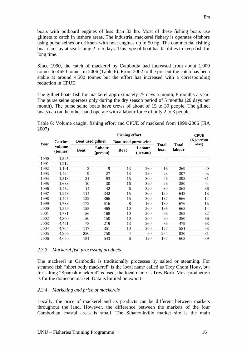
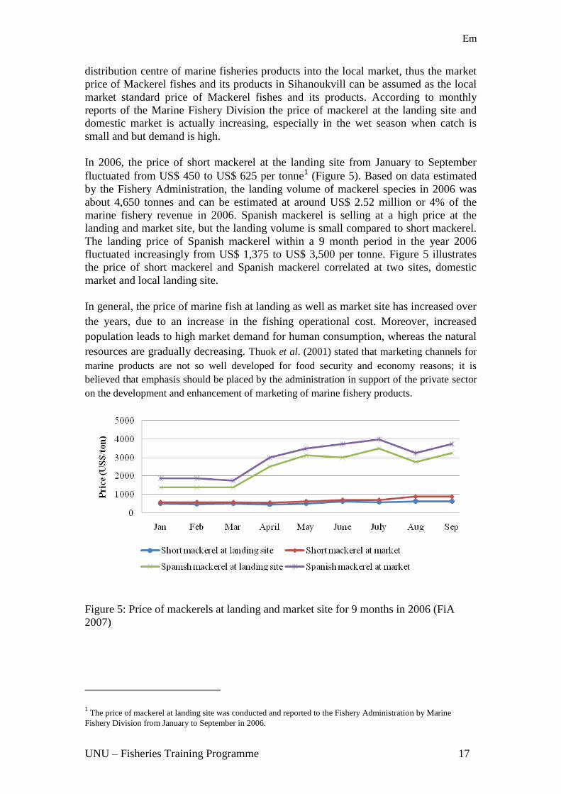
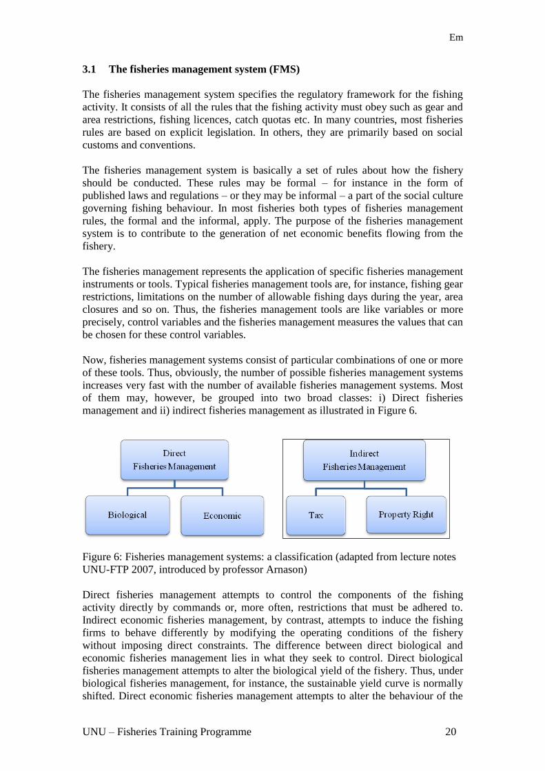
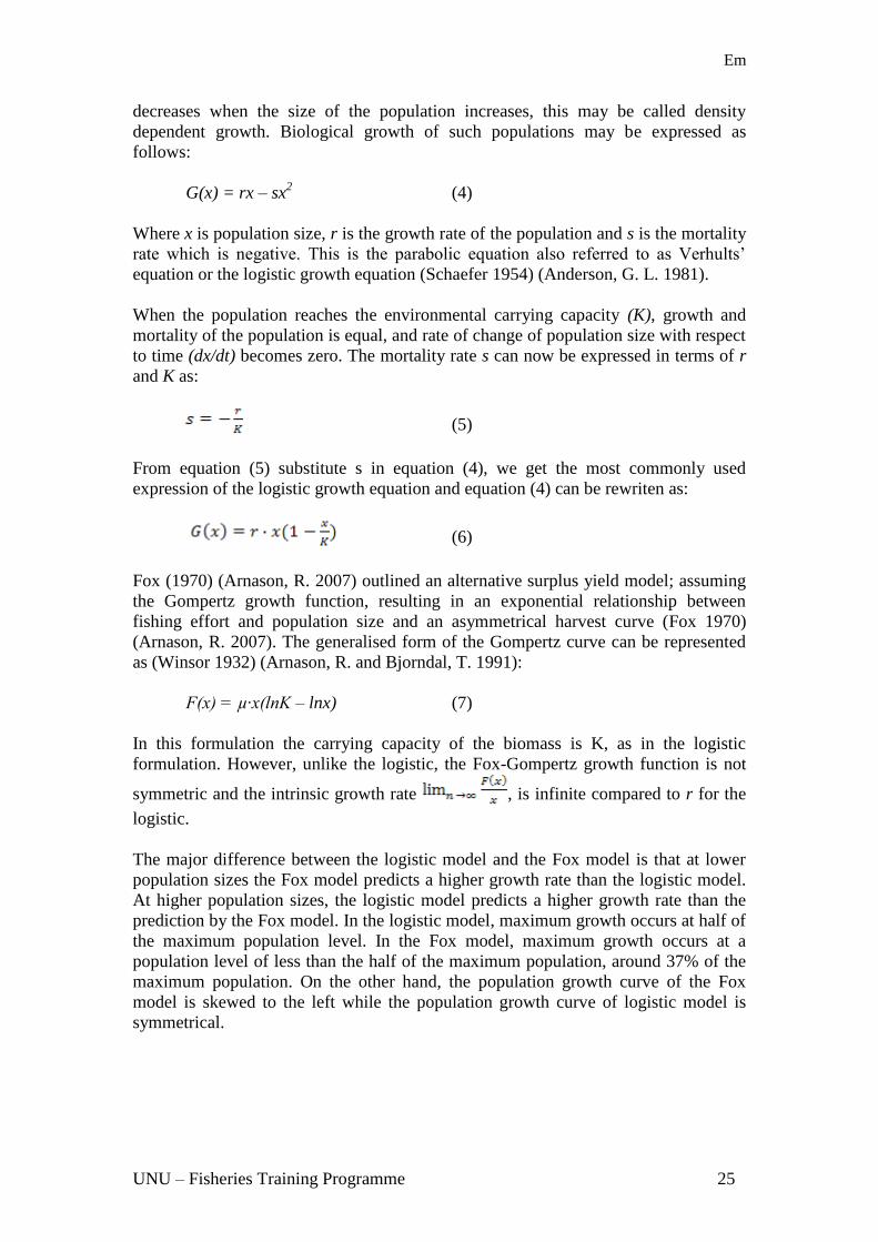
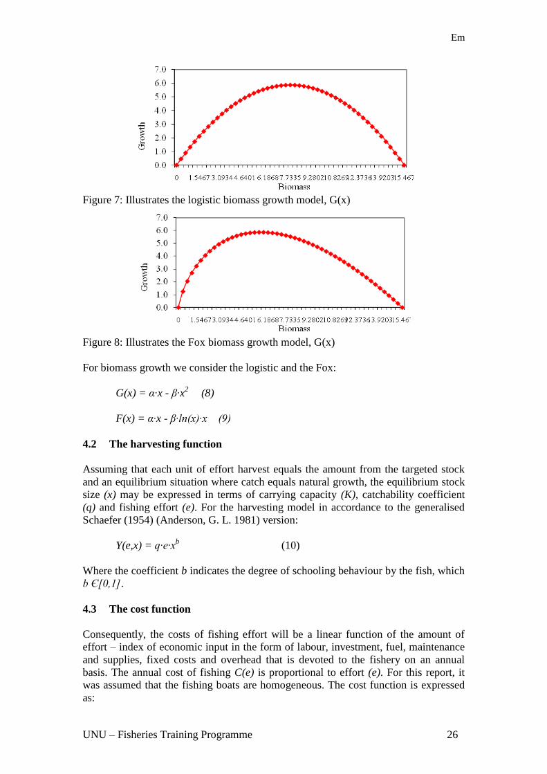

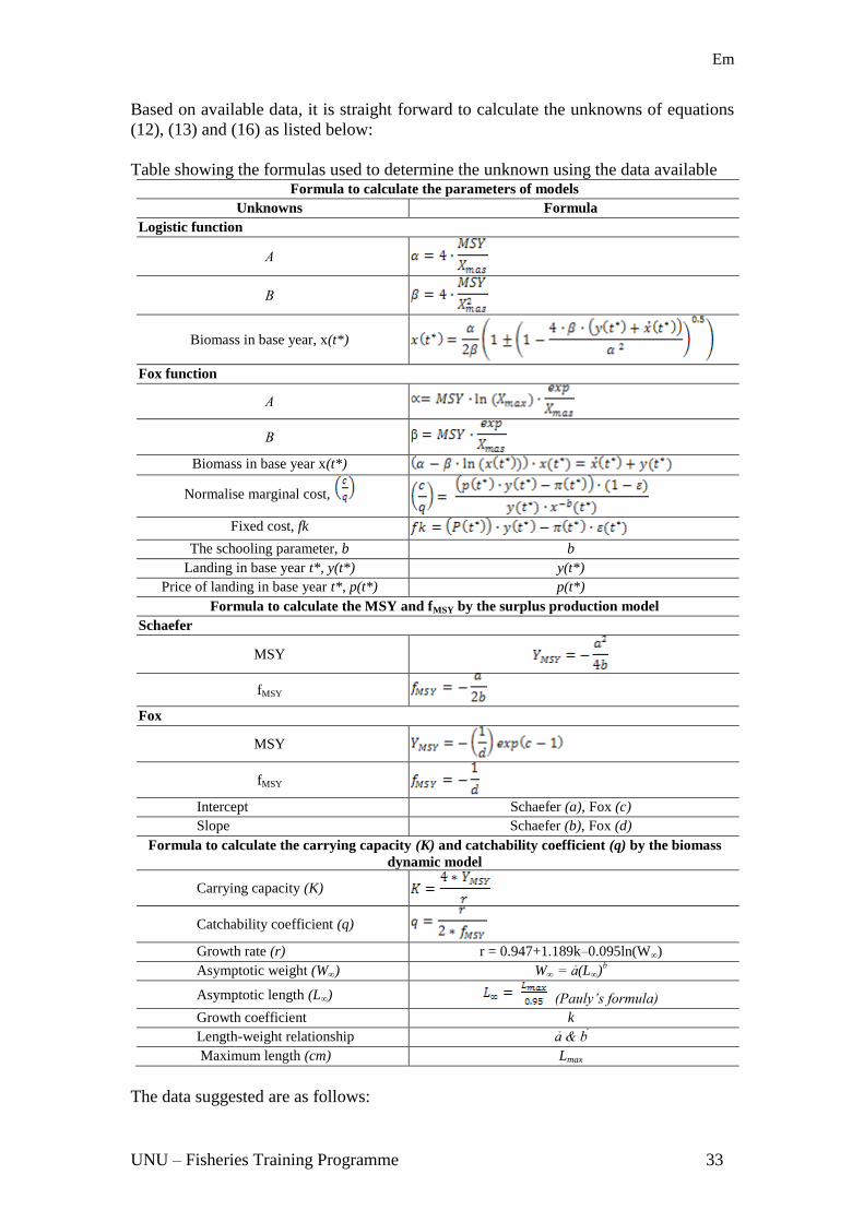
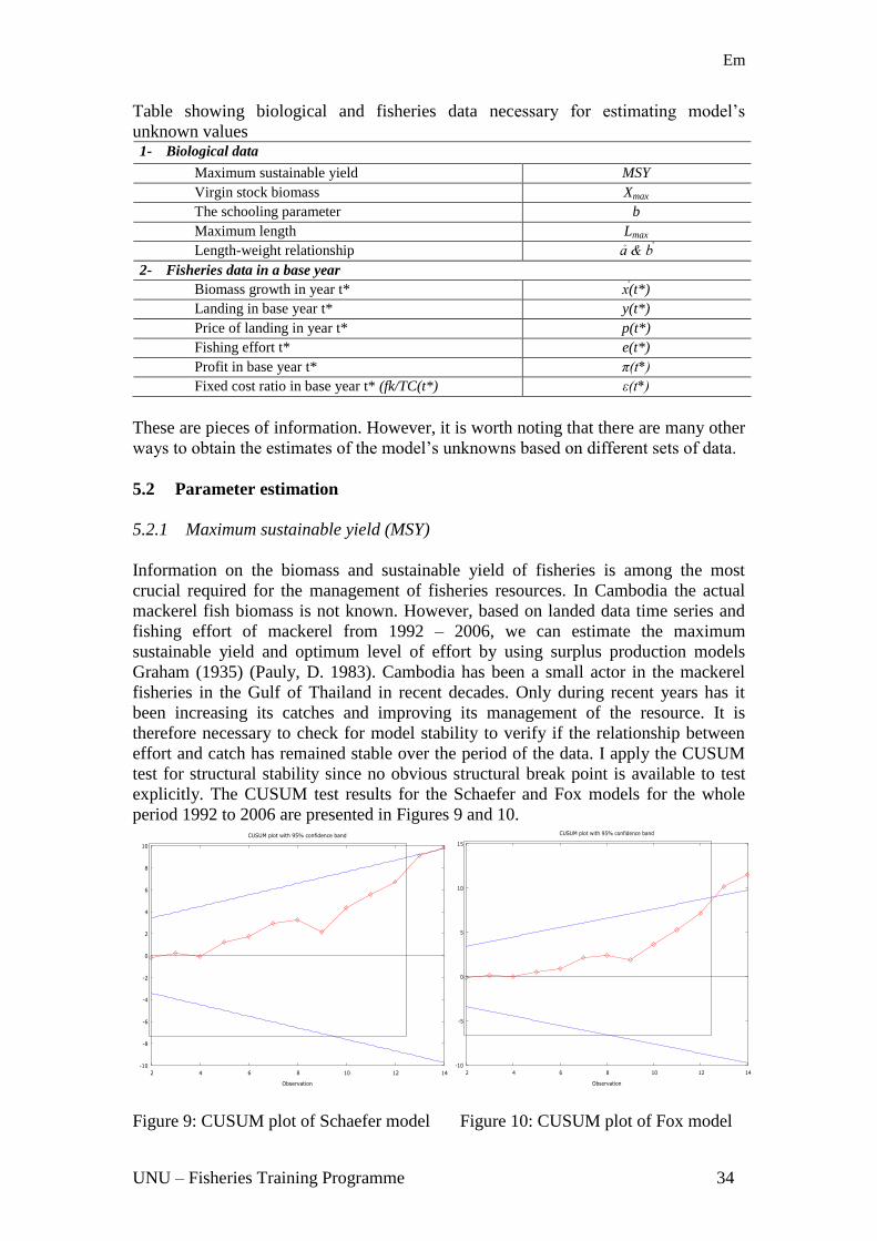
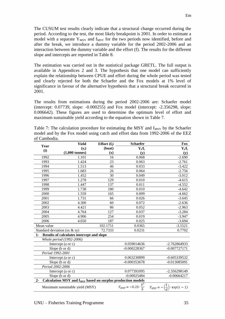
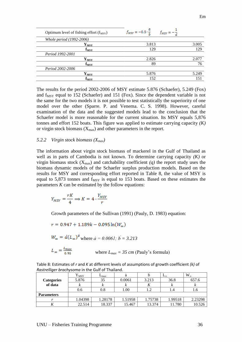
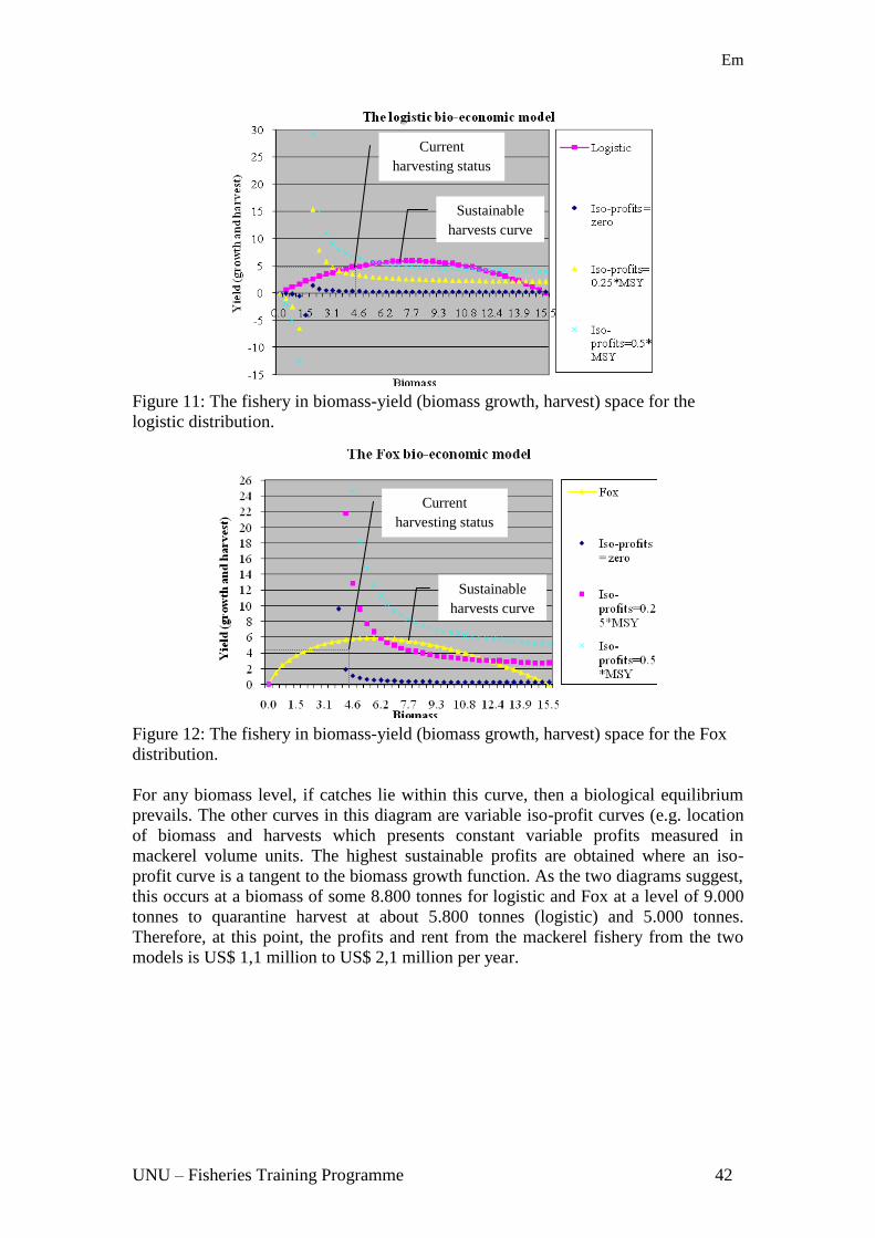
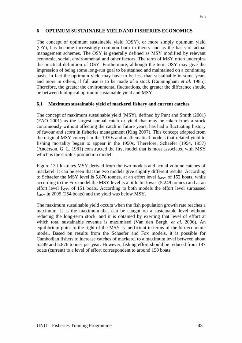
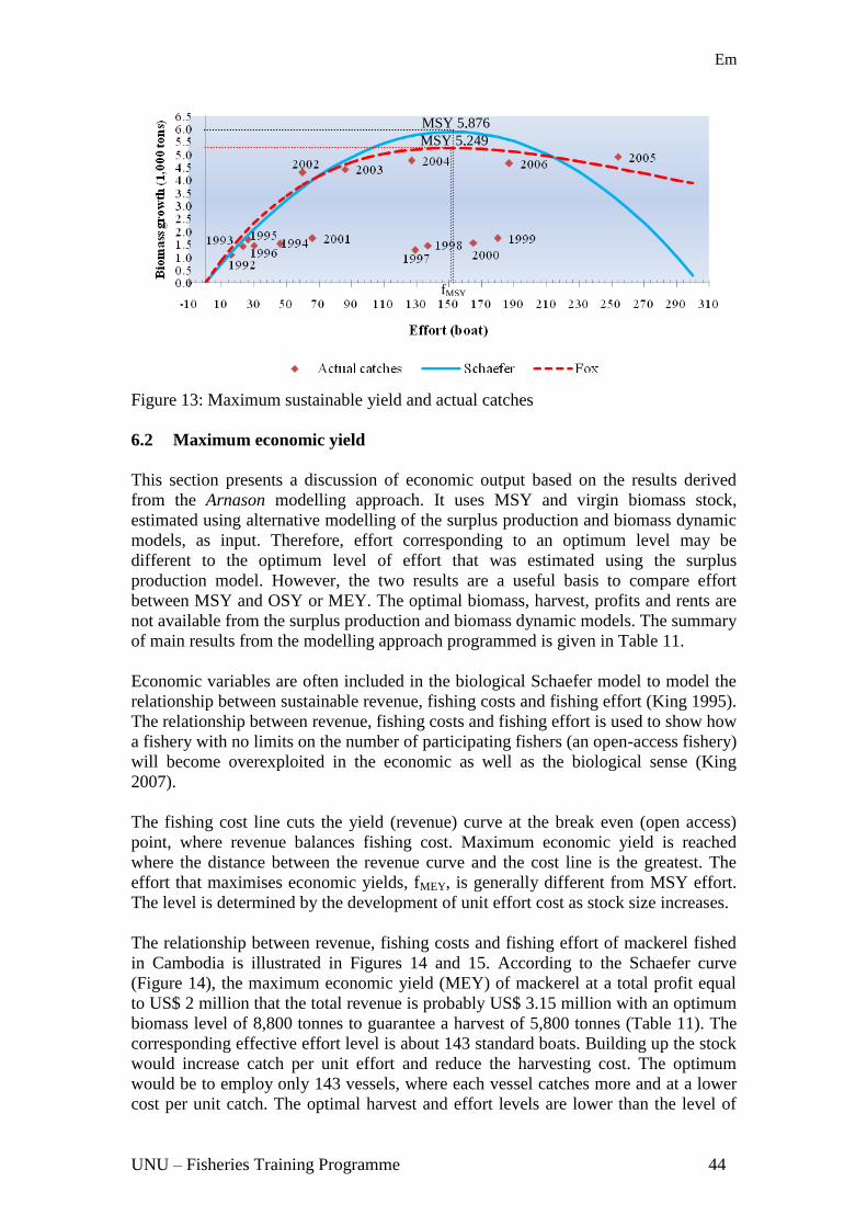
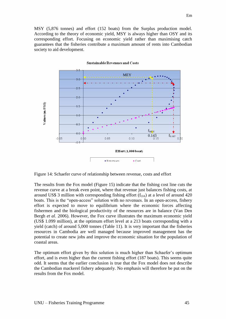
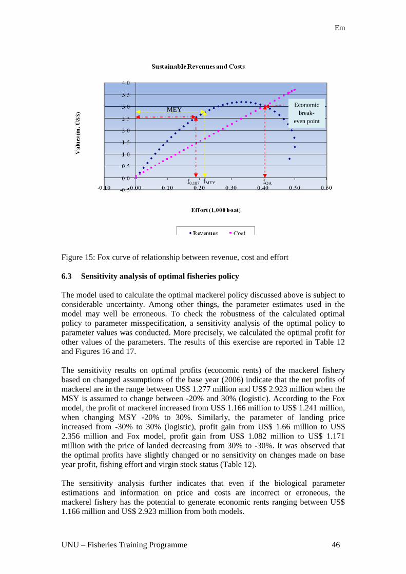
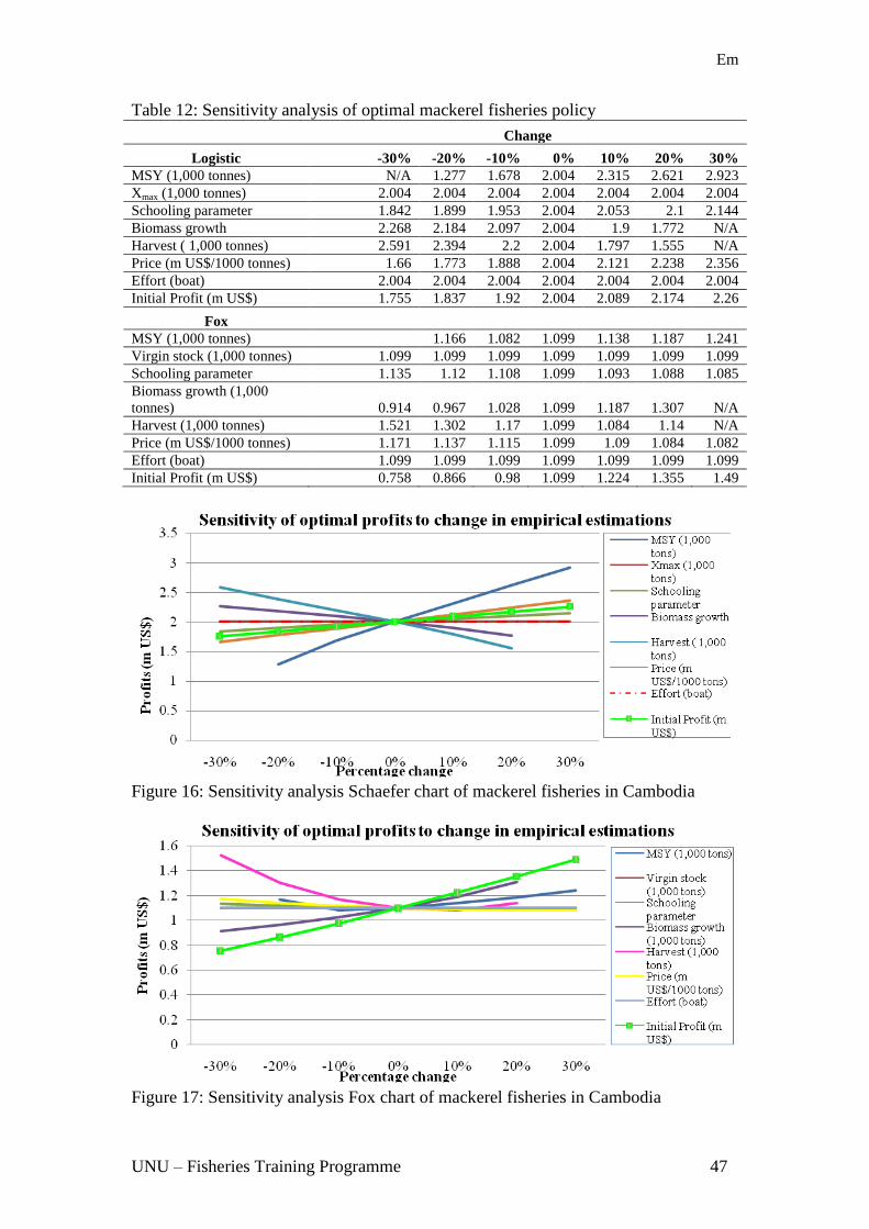
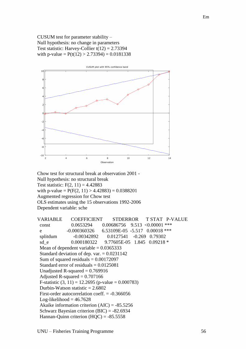
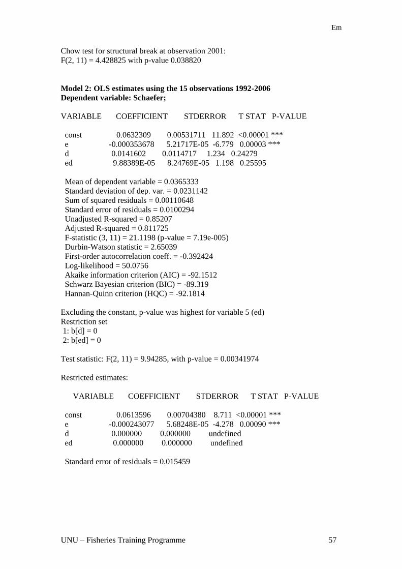
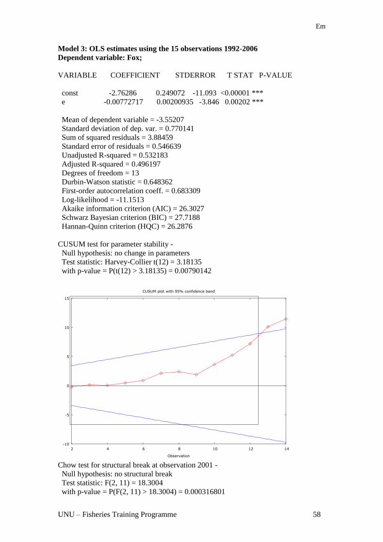
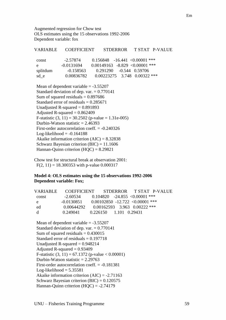
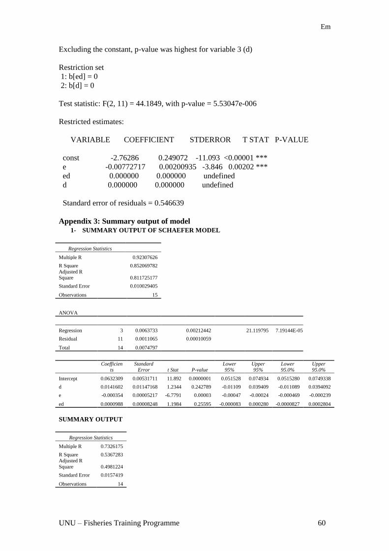
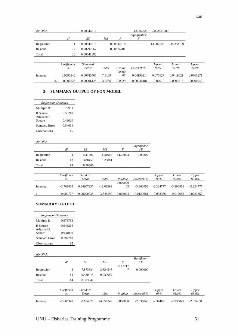
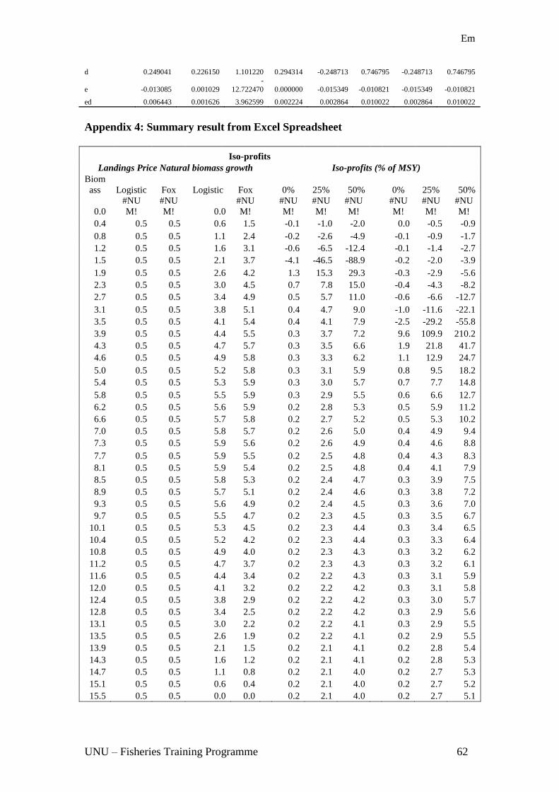
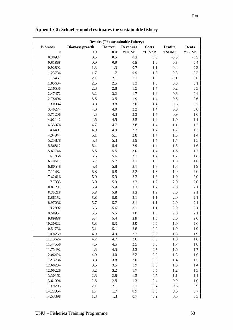
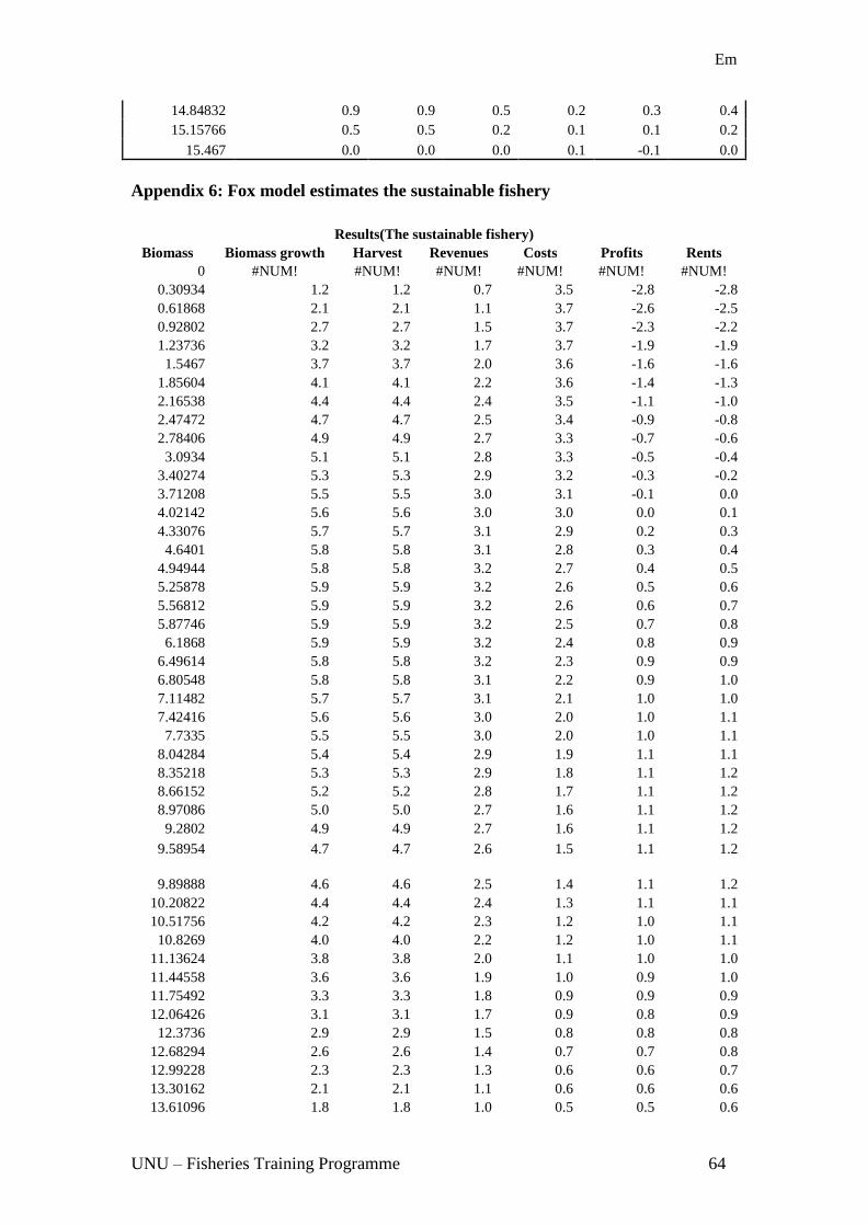
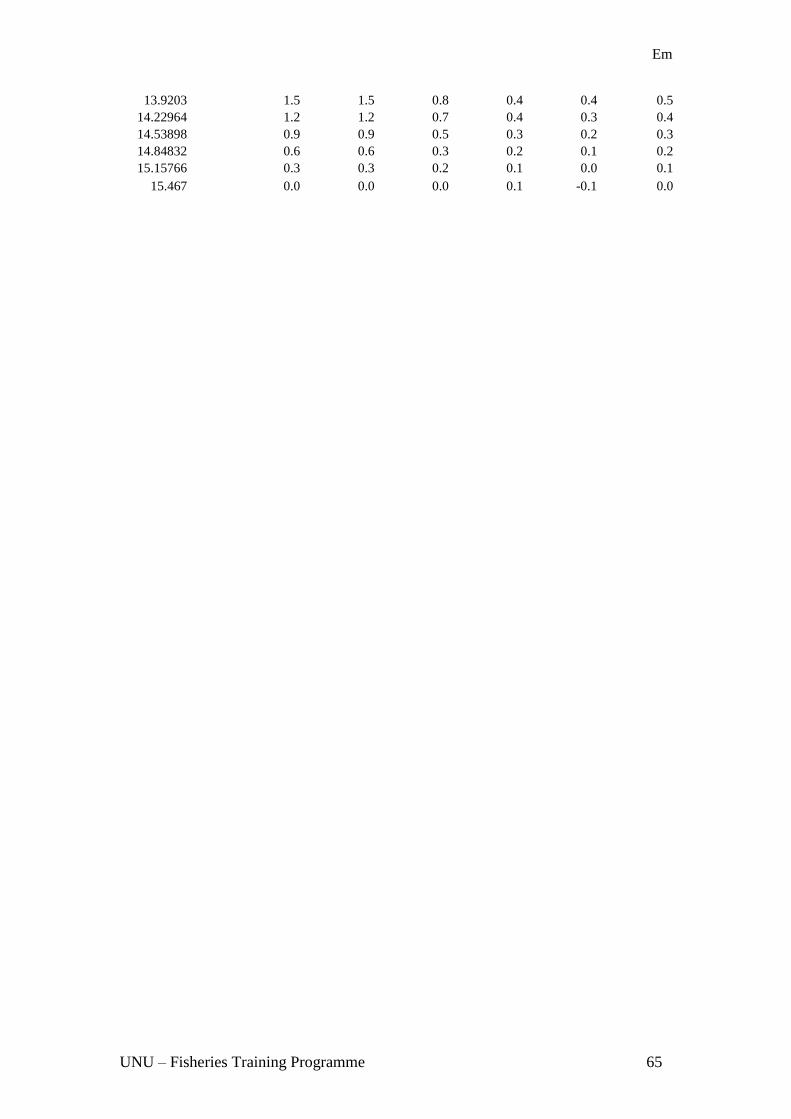


![NATIONAL MARINE FISHERIES SERVICE …...NATIONAL MARINE FISHERIES SERVICE INSTRUCTIONS 01-101-03 [9/30/2015] Fisheries Management Fisheries Management Actions, NMFSPD -01-101 OPERATIONAL](https://static.fdocuments.in/doc/165x107/5f0d46657e708231d4398972/national-marine-fisheries-service-national-marine-fisheries-service-instructions.jpg)


