Marginal Estimation of Parameter Driven Binomial Time ... · Marginal Estimation of Parameter...

Marginal Estimation of Parameter Driven Binomial

Time Series Models

W.T.M. DunsmuirSchool of Mathematics and Statistics, University of New South Wales, Sydney, Australia.

[email protected]

J.Y. HeSchool of Mathematics and Statistics, University of New South Wales, Sydney, Australia

[email protected]

Abstract: This paper develops asymptotic theory for estimation of parameters in regression modelsfor binomial response time series where serial dependence is present through a latent process. Useof generalized linear model (GLM) estimating equations leads to asymptotically biased estimates ofregression coefficients for binomial responses. An alternative is to use marginal likelihood, in whichthe variance of the latent process but not the serial dependence is accounted for. In practice this isequivalent to using generalized linear mixed model estimation procedures treating the observationsas independent with a random effect on the intercept term in the regression model. We prove thismethod leads to consistent and asymptotically normal estimates even if there is an autocorrelatedlatent process. Simulations suggest that the use of marginal likelihood can lead to GLM estimatesresult. This problem reduces rapidly with increasing number of binomial trials at each time point but,for binary data, the chance of it can remain over 45% even in very long time series. We provide acombination of theoretical and heuristic explanations for this phenomenon in terms of the propertiesof the regression component of the model and these can be used to guide application of the methodin practice.

Keywords and phrases: Binomial time series regression, Parameter driven models, Marginal likeli-hood.

1. Introduction

Discrete valued time series are increasingly of practical importance with applications in diverse fields such asanalysis of crime statistics, econometric modelling, high frequency financial data, animal behaviour, epidemi-ological assessments and disease outbreak monitoring, and modern biology including DNA sequence analysis– see Dunsmuir, Tran and Weatherburn (2008). In this paper we focus on time series of binomial counts.

Two broad classes of models for time series of counts, based on the categorization of Cox (1981), aregenerally discussed in the literature: observation driven models, in which the serial dependence relies on pre-vious observations and residuals; and parameter driven models, in which the serial dependence is introducedthrough an unobserved latent process. Estimation of parameter driven models is significantly challengingespecially when the latent process is correlated. Therefore methods that provides preliminary informationof the regression parameters without requiring a heavy computation load would be appealing. For example,the use of generalized linear model (GLM) estimation for obtaining estimates of the regression parameters isdiscussed in Davis, Dunsmuir and Wang (2000) and Davis and Wu (2009) for Poisson and negative binomialobservations respectively. GLM estimation is consistent and asymptotically normal for these two types ofresponse distribution even when there is a latent process inducing serial dependence. However as recentlypointed out by Wu and Cui (2014) and discussed in more detail below, use of GLM for binary or binomialdata leads to asymptotically biased estimates. Wu and Cui (2014) propose a semiparametric estimationmethod for binary response data in which the marginal probability of success modelled non-parametrically.This paper takes a different approach and suggest using estimation based on one-dimensional marginal distri-butions which accounts for the variance of the latent process but not the serial dependence. Such a procedureis easy to implement using standard software for fitting generalized linear mixed models (GLMM). We showthat this method leads to estimates of regression parameters and the variance of the latent process, whichare consistent and asymptotically normal even if the latent process includes serial dependence. Additionallythe method extends easily to other response distributions such as the Poisson and negative binomial and in

1

arX

iv:1

606.

0097

6v1

[m

ath.

ST]

3 J

un 2

016

/Marginal Estimation of Binomial Time Series Mixed Models 2

these cases will improve efficiency of regression parameters related to GLM estimates.Suppose Yt represents the number of successes in mt trials observed at time t. Assume that there are n

observations y1, . . . , yn from the process Yt and that xnt is an observed r-dimensional vector of regressors,which may depend on the sample size n to form a triangular array, and whose first component is unity foran intercept term. Then given xnt and a latent process αt, the Yt are independent with density

fYt(yt|xnt, αt; θ) = exp ytWt −mtb(Wt) + c(yt) (1)

in whichWt = xT

ntβ + αt, (2)

and b(Wt) = log(1 + exp(Wt)) and c(yt) = log(mt

yt

). Then

E(Yt|xnt, αt) = mtb(Wt), Var(Yt|xnt, αt) = mtb(Wt).

The process αt is not observed and because of this is referred to as a latent process. Often αt is assumedto be a stationary Gaussian linear process with zero mean and auto-covariances

Cov (αt, αt+h) = τR(h;ψ)

where τ is the marginal variance of αt and ψ are the parameters for the serial dependence in the model ofαt. The specification of stationary Gaussian linear process covers many practical applications and we willassume that for the remainder of the paper. However, Gaussianity it not required for the main asymptoticresults presented here, and in general, αt can be assumed a stationary strongly mixing process. We willdiscuss this extension further in Section 6.

We let θ = (β, τ, ψ) denote the collection of all parameters and let θ0 be the true parameter vector. Forthe above model the likelihood is defined in terms of an integral of dimension n as follows,

L(θ) :=

∫Rn

n∏t=1

exp ytWt −mtb(Wt) + c(yt) g(α; τ, ψ)dα (3)

where g(α; τ, ψ) is the joint density of α = (α1, . . . , αn) given the parameters τ and ψ.Maximization of the likelihood (3) is computationally expensive. Methods for estimating the high di-

mensional integrals in (3) using approximations, Monte Carlo method or both are reviewed in Davis andDunsmuir (2015). However simple to implement methods that provide asymptotically normal unbiased esti-mators of β and τ without the need to fit the full likelihood are useful for construction of statistics needed toinvestigate the strength and form of the serial dependence. They can also provide a initial parameter valuesfor the maximization of the full likelihood (3).

For practitioners, GLM estimation has strong appeal as it is easy to fit with standard software pack-ages. GLM estimators of the regression parameters β are obtained by treating the observations yt as beingindependent with Wt = xT

ntβ and using the GLM log-likelihood

l0(β) := logL0(β) =

n∑t=1

[yt(xT

ntβ)−mtb(xT

ntβ) + c(yt)] (4)

We let β denote value of β which maximises (4). This GLM estimate assumes that there is no additionalunexplained variation in the responses beyond that due to the regressors xnt.

However, as recently noted by Wu and Cui (2014), GLM does not provide consistent estimates of β whenWt contains a latent autocorrelated component. To be specific, for deterministic regressors xnt = h(t/n) forexample, n−1l0(β) has limit

Q(β) = m

∫ 1

0

(∫Rb(h(u)Tβ0 + α)g(α; τ0)dα(h(u)Tβ)− b(h(u)Tβ)

)du+

M∑m=1

κm

m∑j=0

∫ 1

0

π0(j)c(j)du


where m = E(mt), κm = P (mt = m) and π0(j) = P (Yt = j|xnt, θ0). We show below that β converges to β′,which maximizes Q(β). Equivalently β′ is the unique vector that solves

m

∫ 1

0

(∫Rb(h(u)Tβ0 + α)g(α; τ0)dα− b(h(u)Tβ′)

)h(u)du = 0 (5)

In the Poisson or negative binomial cases, mt ≡ 1, and E(Yt) = E(b(xTntβ0 +αt)) = b(xTntβ0 + τ

2 ), in whichτ/2 only modifies the regression intercept but does not influence the response to other regression terms. Suchan identity does not usually hold for binomial observations. When τ0 > 0, the relationship between β′ andβ0 in binomial logit regression models has been investigated by several researchers. For example, Neuhaus,

Kalbfleisch and Hauck (1991) proved that the logit of the marginal probability∫

(1 + e−(xT β0+α))−1g(α)dαcan be approximated with xTβ∗, where |β∗| ≤ |β0| for single covariate x and the equality is only attainedwhen τ = 0 or β0 = 0. Wang and Louis (2003) proved that only if g(·) is the “bridge” distribution, the

logit of∫

(1 + e−α−xT β0)−1g(α)dα equals to xTβ0 holds; Wu and Cui (2014) proposed their MGLM method

because GLM estimates for binomial observations generated under model (2) are inconsistent.To overcome the inconsistency observed in GLM estimation, in this paper we propose use of marginal

likelihood estimation, which maximises the likelihood constructed under the assumptions that the process αtconsists of independent identically distributed random variables. Under this assumption the full likelihood(3) is replaced by the “marginal” likelihood

L1(δ) =

n∏t=1

f(yt|xt, δ) =

n∏t=1

∫R

exp (ytWt −mtb(Wt) + c(yt)) g(αt; τ)dαt. (6)

and the corresponding “marginal” log-likelihood function is

l1(δ) =

n∑t=1

log f(yt|xt, δ) =

n∑t=1

log

∫R

exp (ytWt −mtb(Wt) + c(yt)) g(αt; τ)dαt. (7)

where δ = (β, τ) and g(·, τ) is the density for a mean zero variance τ normal random variable. Let δ bethe estimates obtained by maximising (7) over the compact parameter space Θ := β ∈ Rr : ‖β − β0‖ ≤d1

⋂τ ≥ 0 : |τ − τ0| ≤ d2, where d1 <∞, d2 <∞.

Marginal likelihood estimators of δ can be easily obtained with standard software packages for fittinggeneralized linear mixed models. Since these marginal likelihood estimates δ are consistent, they can be usedas the starting value of full likelihood based on (3). Additionally, the asymptotic distribution of δ, and thestandard deviation derived from the asymptotic covariance matrix can be used to assess the significance ofregression parameters β. Moreover, in another paper we have developed a two-step score-type test to firstdetect the existence of a latent process and if present whether there is serial dependence. The asymptoticresults of this paper are needed in order to derive the large sample chi-squared distribution of the secondstep, the score test for detecting serial dependence.

Large sample properties of the marginal likelihood estimates δ are provided in Section 2; The simulationsof Section 4 show that marginal likelihood estimates lead to a high probability of τ = 0 when the numberof trials, mt, is small. In particular P (τ = 0) can be almost 50% for binary data. Hence Section 3 focuseson obtaining asymptotic approximations to the upper bound for P (τ = 0), which is useful to quantify theproportion of times the marginal likelihood procedures ‘degenerates’ to the GLM procedure. Also in Section3 we derive a theoretical mixture distribution which provided better approximation in this situation. Section4 presents simulation evidence to demonstrate the accuracy of the asymptotic theory and the covariancematrix of the marginal likelihood estimate. Section 5 discusses the difference between marginal likelihoodestimation and MGLM estimation of Wu and Cui (2014). Section 6 concludes.

2. Asymptotic Theory for Marginal Likelihood Estimates

We present the large sample properties for the marginal likelihood estimates of β and τ obtained by maxi-mizing (7). We begin by presenting the required conditions on the latent process αt, the regressors xntand the sequence of binomial trials mt.


A process αt is strongly mixing if

ν(h) = supt

supA∈Ft

−∞,B∈F∞t+h

|P (AB)− P (A)P (B)| → 0

as h→∞, where Ft−∞ and F∞t+h are the σ-fields generated by αs, s ≤ t and αs, s ≥ t+ h respectively.In practice, the number of trials mt may vary with time. To allow for this we introduce:

Condition 1. The sequence of trials mt : 1 ≤ mt ≤M is a stationary strongly mixing process independent

to Xt; the mixing coefficients satisfy:∞∑h=0

ν(h) <∞. Let κj = P (mt = j), assume κM > 0,M∑j=1

κj = 1.

An alternative would be to take mt as deterministic and asymptotically stationary in which case the κjwould be limits of finite sample frequencies of occurrences mt = j. Both specifications obviously include thecase where mt = M for all t, of which M = 1 yields binary responses.

As in previous literature Davis, Dunsmuir and Wang (2000), Davis and Wu (2009) and Wu and Cui (2014)we allow for both deterministic and stochastic regressors:

Condition 2. The regression sequence is specified in one of two ways:

(a) Deterministic covariates defined with functions: xnt = h(t/n) for some specified piecewise continuousvector function h : [0, 1]→ Rr.

(b) Stochastic covariates which are a stationary vector process: xnt = xt for all n where xt is an observed

trajectory of a stationary process for which E(esTXt) <∞ for all s ∈ Rr.

Condition 3. Let r = dim(β). The regressor space X = xnt : t ≥ 1, assume rank(span(X)) = r.

The full rank of the space spanned by the regressors required for Condition 3 holds for many examples. Forinstance, for deterministic regressors generated by functions given in Condition 2a, such Xi, i = 1, . . . , r existif there are r different values of ui = (u1, . . . , ur) such that the corresponding function (h(u1), . . . , h(ur)) arelinearly independent. For stochastic regressors generated with a stationary process given in Condition 2b,linearly independent Xi, i = 1, . . . , r can be found almost surely if Cov(X) > 0.

Condition 4. The latent process αt, is strictly stationary, Gaussian and strongly mixing with the mixingcoefficients satisfying

∑∞h=0 ν(h)λ/(2+λ) <∞ for some λ > 0.

Conditions for a unique asymptotic limit of the marginal likelihood estimators are also required. Denotethe marginal probability of j successes in mt trials at time t as

πt(j) =

∫RejWt−mtb(Wt)+c(j)φ(zt)dzt, j = 1, . . . ,mt.

where Wt = xTntβ + τ1/2zt, and zt = αt/τ1/2 has unit variance. If αt is Gaussian, so is the process zt

and zt ∼ N(0, 1) with density function φ(·). Similarly let π0t (j) be the marginal probability evaluated with

the true values β0 and τ0 at time t. Define

Qn(δ) =1

nl1(δ) (8)

conditional on mt and xnt,

E(Qn(δ)) =1

n

n∑t=1

mt∑j=0

π0t (j) log πt(j), δ ∈ Θ. (9)

Under Conditions 1 and 2, E(Qn(δ))a.s.→ Q(δ). Let π(j, ·) = P (Y = j|·, δ), and π0(j, ·) is evaluated with

δ0, then under Condition 2a,

Q(δ) =

M∑m=1

κm

∫ 1

0

m∑j=0

π0(j, h(u)) log π(j, h(u))du (10)


and, under Condition 2b,

Q(δ) =

M∑m=1

κm

∫Rr

m∑j=0

π0(j, x) log π(j, x)dF (x) (11)

the proof is included in the proof of Theorem 1.

Condition 5. Q(δ) has a unique maximum at δ0 = (β0, τ0), the true value.

We now establish the consistency and asymptotic normality of the marginal likelihood estimator.

Theorem 1 (Consistency and asymptotic normality of marginal likelihood estimators). Assume τ0 > 0 and

Conditions 1 to 5, then δa.s.→ δ0 and

√n(δ − δ0)

d→ N(0,Ω−11,1Ω1,2Ω−1

1,1) as n→∞, in which

Ω1,1 = limn→∞

1

n

n∑t=1

E(lt(δ0)lTt (δ0)) > 0 (12)

Ω1,2 = limn→∞

1

n

n∑t=1

n∑s=1

Cov(lt(δ0), ls(δ0)) (13)

where

lt(δ0) =∂ log πt(yt)

∂δ|δ0 = f−1(yt|xnt, δ0)

∫(yt −mtb(x

T

ntβ0 + τ1/20 zt))

(xntzt

2√τ0

)f(yt|xnt, zt, δ0)φ(zt)dzt (14)

To use this theorem in practice requires at least that the identifiability condition holds and that thecovariance be estimated from a single series. We address these aspects in detail in Section 2.1 and 2.2.In addition, particularly for binary responses, marginal likelihood estimators produce a high probability ofτ = 0. We address this in detail in Section 3, where we propose an improved asymptotic distribution basedon a mixture.

2.1. Asymptotic identifiability

We now discuss circumstances under which Condition 5 holds. Now for any δ ∈ Θ, Q(δ) ≤ Q(δ0), since forany x,

∑mj=0 π

0(j, x) log π(j, x) ≤∑mj=0 π

0(j, x) log π0(j, x). Thus the model is identifiable if and only if forany δ ∈ Θ, Q(δ)−Q(δ0) < 0 if δ 6= δ0.

Lemma 1. Assume M ≥ 2 and Condition 3, then Condition 5 holds for marginal likelihood (7).

The proof is outlined in Appendix A.

For binary data, M = 1, then Q(δ) = Q(δ0) if π(1, x) = π0(1, x), ∀x ∈ X. Hence model (7) is notidentifiable if ∃δ 6= δ0 such that π(1) = π0(1) everywhere on X, that is, for each distinct value Xi ∈ X, such(β, τ) 6= (β0, τ0) can be found to establish

π(1, Xi) =

∫eX

Ti β+

√τz

1 + eXTi β+

√τzφ(z)dz =

∫eX

Ti β0+

√τ0z

1 + eXTi β0+

√τ0z

φ(z)dz = π0(1, Xi). (15)

If τ = τ0, then (15) implies XTi β = XT

i β0. Under Condition 3, r linearly independent Xi, X = (X1, . . . , Xr)can be found on X to establish XTβ = XTβ0. Then (β − β0) has a unique solution of 0r. Hence if τ = τ0,(15) holds if and only if β = β0, and Condition 5 holds.

If τ 6= τ0, for each Xi, a unique solution of ai, ai = XTi β 6= XT

i β0 can be found for (15). Assume theregressor space X is a set of discrete vectors such that X = Xi : 1 ≤ i ≤ L, where Xi 6= Xj if i 6= j. LetX = (X1, . . . , XL) be a r×L matrix. Then (15) holds for each Xi ∈ X if there exists such solution of β thatXTβ = A, A = (a1, . . . , aL). Since τ 6= τ0, β = β0 is not excluded from the possible solutions of β. If L = r,a unique solution of β exists, hence there exists such δ 6= δ0 that establishes (15) for all Xi ∈ X, therefore(7) is not identifiable. If L > r, note rank(X) = r, then XTβ = A is overdetermined. Thus a solution ofβ does not always exist and in these situations Condition 5 holds, however a general proof without furtherconditions on the regressors is difficult. Instead, we provide a rigourous proof to show Condition 5 holds forbinary data when the regressor space X is connected.


Lemma 2. Let M = 1. In addition to Condition 3, X is assumed to be a connected subspace of Rr, thenCondition 5 holds.

Proof: see the appendix A.

2.2. Estimation of the Covariance matrix

To use Theorem 1 the asymptotic covariance matrix Ω−11,1Ω1,2Ω−1

1,1 needs to be estimated using a singleobserved time series. Now Ω1,1 can be estimated by replacing δ0 with the marginal likelihood estimates

δ. However estimation of Ω1,2 is challenging, as Ω1,2 = n−1E[∑n

t=1

∑ns=1 lt(δ0)ls(δ0)

]has cross terms

E(lt(δ0)ls(δ0)

), s 6= t, which cannot be estimated without knowledge of ψ0. We use the modified subsampling

methods reviewed in Wu (2012) and Wu and Cui (2014) to estimate Ω1,2.Let Yi,kn = (yi, . . . , yi+kn−1) denote the subseries of length kn starting at the ith observation, where

i = 1, . . . ,mn and mn = n− kn + 1 is the total number of subseries. Define

qn,t =1√nlt(δ)

by replacing δ0 by δ in (14). Under similar conditions to those given above, we show that as kn → ∞ and

mn →∞, Γ−11,nΓ†nΓ−1

1,n is a consistent estimator of the asymptotic covariance matrix of δ, where

Γ1,n =

n∑t=1

qn,tqT

n,t; Γ†n =1

mn

mn∑i=1

(i+kn−1∑t=i

i+kn−1∑s=i

qkn,tqT

kn,s

)The performance of subsampling estimators relies on kn to a large extent. Following the guidance of Heagertyand Lumley (2000) on optimal selection of kn, we use kn = C[n1/3], C = 1, 2, 4, 8 in the simulations. Theone dimensional integrals in qn,t can be easily obtained using the R function integrate.

3. Degeneration of Marginal Likelihood Estimates

Even when the identifiability conditions are satisfied, in finite samples the marginal likelihood can be max-imised at τ = 0, in which case β degenerates to the ordinary GLM estimate β. Simulation evidence ofSection 4 suggests that the chance of this occurring, even for moderate to large sample sizes, is large (upto 50% for binary data but decreasing rapidly as the number of trials m increases). In this section we willderive two approximations for this probability. In both approximations we conclude that P (τ = 0) will behigh whenever the range of xT

ntβ is such that b(xTntβ) ≈ a0 + a1(xT

ntβ), where a0, a1 are constants. Whenthis linear approximation is accurate the covariance matrix for the marginal likelihood estimates is obtainedfrom the inverse of a near singular matrix and results in var(τ) being very large so that P (τ = 0) is close

to 50%. When there is a nontrivial probability of τ = 0, the distribution of β for finite samples is betterapproximated by a mixture of two multivariate distributions weighted by P (τ = 0) and P (τ > 0).

3.1. Estimating the probability of τ = 0

One approximation for the probability of τ = 0 can be obtained using the asymptotic normal distributionprovided in Theorem 1. Define κ2 = P (

√n(τ − τ0) ≤ −

√nτ0), then in the limit,

κ2 = Φ(−√nτ0/στ (δ0)); σ2

τ (δ0) = (Ω−11,1Ω1,2Ω−1

1,1)ττ (16)

where Φ(·) is the standard normal distribution.An alternative approximation to P (τ = 0) can be based on the score function evaluated at τ = 0. Consider

the scaled score function S1,n(β) = 2n−1∂l1(β, τ)/∂τ |β=β,τ=0, which, using integration by parts, is

S1,n(β) =1

n

n∑t=1

[(yt −mtb(x

T

ntβ))2 −mtb(xT

ntβ)]. (17)


Now, τ = 0 implies S1,n(β) ≤ 0 but not the converse, hence P (τ = 0) is bounded above by P (S1,n(β) ≤ 0).In order to derive a large sample approximation to this probability we show, in Section 3.2, that the

large sample distribution of√n(S1,n(β) − cS)/σS is standard normal, where cS = lim

n→∞E(S1,n(β′)) and

σ2S = lim

n→∞Var(√nS1,n(β)). Define κ1 = P (S1,n(β) ≤ 0), it can then be approximated with

κ1 = Φ(−√ncS/σS). (18)

The quantities cS and σS can be expressed analytically for some regression specifications. In simulations,the limits are computed using numerical integration. For the binary case in particular, the ratio cS/σS canbe quite small resulting in a large value for κ1. We compare how well P (τ = 0) is estimated by κ1 and κ2

via simulations in Section 4, and conclude that κ1 is slightly more accurate in the situation covered there.

3.2. Asymptotic Theory for GLM Estimates and Marginal Score

To develop the asymptotic distribution of S1,n(β), the asymptotic normality of√n(β − β′) is required.

Theorem 2 (Asymptotic normality of GLM estimators). Under Conditions 1 to 4, the estimates β max-

imising the likelihood (4) satisfies βp→ β′, and

√n(β − β′)→ N(0,Ω−1

1 Ω2Ω−11 ) as n→∞, in which

Ω1 = limn→∞

1

n

n∑t=1

mtb(xTntβ′)xntx

T

nt

Ω2 = limn→∞

1

n

n∑t=1

n∑s=1

mtms

(∫(b(xT

ntβ0 + αt)− b(xT

ntβ′))(b(xT

nsβ0 + αs)− b(xT

nsβ′))g(αt, αs; τ0, ψ0)dα

)xntx

T

ns

+ limn→∞

1

n

n∑t=1

mt

(∫b(xT

ntβ0 + αt)g(αt; τ0)dα

)xntx

T

nt

The proof of this theorem is given in Appendix B. It relies on concavity of the GLM log likelihood withrespect to β. Standard results of a functional limit theorem are used to establish the above result, in a similarway as that used in Davis, Dunsmuir and Wang (2000), Davis and Wu (2009) and Wu and Cui (2014).

In order to use Theorem 2 for practical purposes, first β′ needs to be determined and then Ω1, Ω2.Estimation of β′ would require knowledge of τ , and the estimation of Ω2 would require both τ and ψ, neitherof which can be estimated using the GLM procedure. Hence the theorem is of theoretical value only.

Based on Theorem 2 we can now derive the large sample distribution of the score function of the marginal

likelihood evaluated at δ = (β, 0). Because all derivatives of b(·) are uniformly bounded and βp→ β′, hence

√n(S1,n(β)− E(S1,n(β′))

)=√n (S1,n(β′)− E(S1,n(β′)))− JT

S

√n(β − β′) + op(1).

Since n−1/2∑nt=1(yt −mtb(x

Tntβ))xnt = 0 by definition of β, using Taylor expansion

√n(β − β′) = Ω−1

1

1√n

n∑t=1

et,β′xnt + op(1), et,β′ = yt −mtb(xT

ntβ′).

Then it follows that √n(S1,n(β))− E(S1,n(β′))

)− (U1,n − JT

SU2,n)p→ 0 (19)

where

JS = limn→∞

1

n

n∑t=1

[2m2

t (π0(xT

ntβ0)− b(xTntβ′))b(xTntβ′) +mtb(3)(xTntβ

′)]xnt (20)

U1,n :=√n (S1,n(β′)− E(S1,n(β′))) =

1√n

n∑t=1

e2t,β′ − Ee2

t,β′ ; U2,n :=1√n

n∑t=1

et,β′cnt (21)


note π0(xTntβ0) =

∫b(xT

ntβ0 + αt)g(αt, τ0)dα and cnt = Ω−11 xnt, which is a non-random vector.

Then the CLT for√n(S1,n(β)− E(S1,n(β′))

)follows the CLT for the joint vector of (U1,n, U2,n). Note

that both sequences of U1,t and U2,t are strongly mixing by Proposition 1 in Blais, MacGibbon andRoy (2000). Then the CLT for mixing process proposed in Davidson (1992) can be applied to show that(U1,n, U2,n) is asymptotically normally distributed with mean zero and covariance matrix(

VS Ω−11 KS

KT

SΩ−11 Ω−1

1 Ω2Ω−11

)where Ω1,Ω2 are given in Theorem 2, and

VS := limn→∞

(n−1)∑h=0

(1

n

n∑t=1

Cov(e2t,β′ , e

2t+h,β′)

)+

(n−1)∑h=1

(1

n

n∑t=h+1

Cov(e2t,β′ , e

2t−h,β′)

)KS := lim

n→∞

(n−1)∑h=0

(1

n

n∑t=1

E(et,β′e2t+h,β′)xnt

)+

(n−1)∑h=1

(1

n

n∑t=h+1

E(et,β′e2t−h,β′)xnt

)Theorem 3. Under the assumptions of Theorem 2, as n→∞,

√n(S1,n(β)− E(S1,n(β′))

)/σS

d→ N(0, 1).

3.3. An approximate mixture distribution for β

Theorem 4 (Mixture distribution under finite samples). Assume τ0 > 0, under Conditions 1 to 5, in finite

samples, distribution of√n(β − β0) can be approximated with the mixture

κF1(c, δ0) + (1− κ)F2(c, δ0), κ = P (τ = 0)

in which F1(c, δ0) is r-dimensional multivariate distribution obtained through√n(β − β′), which is a skew

normal distribution U2,n|U1,n +√nE(S1,n(β′)) − 2JT

SU2,n ≤ 0, based on the joint normality of (U1,n, U2,n)

given in Theorem 3; F2(c, δ0) is a r-dimensional skew normal distribution√n(β − β0)|τ > 0, based on the

joint normality of N(0,Ω−11,1Ω1,2Ω−1

1,1) in Theorem 1. Moreover, κ→ 0 as n→∞.

Remarks

1. The skew normal distribution is defined in Gupta, Gonzalez-Farıas and Domınguez-Molina (2004).2. If τ0 = 0, β′ = β0 and the value κ = 0.5 in the above mixture is similar to that in Moran (1971,

Theorem I); when τ0 = a/√n, a ≥ 0, above results are parallel to those in Moran (1971, Theorem IV)

and based on the same reasoning. However Moran’s results are for independence observations whereasour results require the serial dependence to be accounted for in the asymptotic results.

3. While the mixture provides a better theoretical description of the asymptotic distribution for marginallikelihood estimates when m is small, in practice, the mixture distribution cannot be estimated withoutknowing the true values of β0, τ0 and ψ0. In simulations, the covariance matrix for the joint distributionof β and τ is approximated with Σ(δ0) = n−1Ω−1

1,1Ω1,2Ω−11,1, and based on F2(c, δ0), we calculate

E(β − β0|τ > 0) = Σβτ (δ0)Σ−1ττ (δ0)E(τ − τ0|τ > 0) (22)

Var(β|τ > 0) = Σββ(δ0)− Σβτ (δ0)Σ−1ττ (δ0)Στβ(δ0) + Σβτ (δ0)Σ−2

ττ (δ0)Στβ(δ0)Var(τ − τ0|τ > 0) (23)

4. Simulation Results

In this section we summarize results of several simulation studies to illustrate the key theoretical resultsderived above as well as to indicate circumstances under which P (τ = 0) is large in which case the mixturedistribution of Theorem 4 would provide a more accurate description.


For all examples we consider the simple linear trend with latent process W0,t = β1 + β2(t/n) + αt, in

which αt is assumed to be: αt = φαt−1 + εt, εti.i.d∼ N(0, σ2

ε ) where σ2ε is chosen to maintain Var(αt) = 1. In

all cases the true values are β0 = (1, 2) and τ0 = 1 and φ varies in the interval (−1, 1). While simple, thisexample provides substantial insights into the behaviour of the marginal likelihood estimates as well as intoproblems that can arise. The simplicity of this example also allows us to obtain analytical calculations ofkey quantities and to provide some heuristic explanations of the non-standard distribution results which canarise, particularly for binary time series.

In all simulations reported later, the number of replications was 10, 000. The marginal likelihood estimateswere obtained using the R package lme4. The frequency with which τ = 0 is not package dependent otherthan the occasionaly case – this was checked using our own implementation based on adaptive Gaussianquadrature and by comparing the results with those from SAS PROC MIXED. The first simulation (Section

4.2) focuses on binary responses and illustrates that the distribution of marginal likelihood estimates δ forthis kind of data converge towards a mixture as proposed in Theorem 4, in which the P (τ = 0) can beapproximated using the result of Theorem 3 to good accuracy. The second experiment (Section 4.3) studies

the finite sample performance of δ for binomial cases and shows that P (τ = 0) vanishes as mt increases or as

n → ∞, thus the distribution of δ is multivariate normal as developed in Theorem 1. Finally (Section 4.4)

the method for estimation the covariance matrix for δ proposed in Section 2.2, is evaluated.In order to implement the simulations in Section 4.1 we first derive some theoretical expressions for key

quantities used to define the large sample distributions of Theorems 1, 2 and 3 as well as for the estimatesκ1 and κ2 for P (τ = 0).

4.1. Analytical Expressions for Asymptotic Quantities

Key quantities required for implementation and explanation of the simulation results to follow are:(1). The limit point β′ for the GLM estimate β.(2). cS and σS appearing in Theorem 3 and used to obtain the approximation κ1 for P (τ = 0).(3). The asymptotic variance of τ in Theorem 1 used to obtain the approximation κ2 for P (τ = 0).(4). Various quantities defining the mixture distribution in Theorem 4.

Throughout, the derivations are given for the case of deterministic regressors specified as xnt = h(t/n)for a suitably defined vector function h as in Condition 2a and in which the first component is unity inorder to include the intercept term. Also, in order to reduce notational clutter we will assume that mt ≡ m(the number of binomial trials at all time points is the same). The analytical expressions involve variousintegrals which are computed using numerical integration either with the R-package integrate or using gridevaluation for u with mesh 0.0001 over the interval [0, 1]. Calculation of Ω1,2 in Theorem 1 and KS , VS andΩ2 in Theorem 3 to obtain the variance σ2

S for the theoretical upper bound of P (τ = 0) require evaluationof two-dimensional integrals of the form

Cov(lt(δ0), lt+h(δ0)) =

mt∑yt=0

mt+h∑yt+h=0

π0(yt, yt+h)lt(δ0)lt+h(δ0).

For these, the integral expression for π0(yt, yt+h) is approximated using adaptive Gaussian quadratic (AGQ)with 9 nodes for each of the two dimensions.

4.1.1. Limit Point of GLM Estimation

By numerically solving the non-linear system (5) with Newton Raphson iteration the limiting value of theGLM estimates is β′ = (0.8206, 1.7574).


4.1.2. Quantities needed for κ1

The analytical expression for the limiting expectation of the scaled score with respect to τ evaluated at thelimiting point β′ is.

cS := limn→∞

E(S1,n(β′))

= limn→∞

1

n

n∑t=1

[m(m− 1)

∫ (b(xT

ntβ0 + αt)− b(xTntβ′))2

g(αt, τ0)dαt +m(b(xT

ntβ′)− π0(xT

ntβ0))(2b(xT

ntβ′)− 1)

]=m(m− 1)

∫ 1

0

∫ (b(h(u)Tβ0 + α)− b(h(u)Tβ′)

)2

g(α, τ0)dαdu

+m

∫ 1

0

(b(h(u)Tβ′)− π0(h(u)Tβ0))(2b(h(u)Tβ′)− 1)du

=m(m− 1)c1 +mc2. (24)

Note that c1 in (24) is strictly positive but make no contribution for binary responses (when m = 1) in whichcase c2 is the only term contributing to cS . We have observed that c2 is non-negative, in the simulations butwe do not have a general proof of that. In that case cS is also non-negative for all m. We have observed inthe simulations that c1 is substantially larger than c2 and as a result κ1 is small for non-binary responses(m > 1) but can be large for binary responses because c2 ≈ 0.

Recall that σ2S = lim

n→∞Var(S1,n(β)). For the case where the latent process is i.i.d. we have

σ2S =

∫ 1

0

mπ0(h(u)Tβ0)(1− π0(h(u)Tβ0))[1 + 2(m− 3)π0(h(u)Tβ0)(1− π0(h(u)Tβ0))

]+4m3π0(h(u)Tβ0)(1− π0(h(u)Tβ0))(π0(h(u)Tβ0)− b(h(u)Tβ′))2

+4m2π0(h(u)Tβ0)(1− π0(h(u)Tβ0))(1− 2π0(h(u)Tβ0))(π0(h(u)Tβ0)− b(h(u)Tβ′))du

−2JTS Ω−11 KS + JTS Ω−1

1 Ω2Ω−11 JS (25)

in which

KS =

∫ 1

0

[mπ0(h(u)Tβ0)(1− π0(h(u)Tβ0))(1− 2π0(h(u)Tβ0))

+ 2m2π0(h(u)Tβ0)(1− π0(h(u)Tβ0))(π0(h(u)Tβ0)− b(h(u)Tβ′))]h(u)du

JS =

∫ 1

0

[2m2(π0(h(u)Tβ0)− b(h(u)Tβ′))b(h(u)Tβ′) +mb(3)(h(u)Tβ′)

]h(u)du

similar expression of σ2S can be obtained for the dependent cases where ψ 6= 0. However, serial dependence

does not appear to make much difference in the chance of τ = 0 at least in the simulations of Section 4.3.For the simulation example of the binary response case (m = 1) the expressions (24), (25) can be evaluated

using numerical integration to give

c1 = 0.0168, c2 = 1.65× 10−5

cS σS cS/σSm = 1 1.65× 10−5 7.17× 10−3 0.0023m = 2 0.034 0.303 0.1110m = 3 0.101 0.525 0.1921

Since cS is observed to be strictly positive for marginal likelihood,√ncS →∞ as n→∞. By Theorem 3,

the probability of S1,n(β) ≤ 0 vanishes as n→∞. Because P (τ = 0) is bounded above by P (S1,n(β) ≤ 0), asn→∞, the marginal likelihood estimate will be such that τ = 0 with vanishing probability. However, noticefor binary data cS = c2 and cS/σS = 0.0023. Hence, even for the largest sample size (n = 5000) reportedbelow, κ1 is 44%. It would require a sample size of 106 to reduce this to 1%. Clearly this has substantial


implications for the use of marginal likelihood for binary data. For binomial responses the c1 term dominates,and hence even with small values of m > 1 the chance of τ = 0 reduces rapidly.

We conclude this subsection with a heuristic explanation of why c2 ≈ 0. If h(u)Tβ′ appearing in thedefinition of c2 is such that b(h(u)Tβ′) is well approximated linearly in h(u)Tβ′ then c2 could be approximatedby

c∗2 =

∫ 1

0

[b(h(u)Tβ′)− π0(h(u)Tβ0)](ao + a1h(u)Tβ′)du. (26)

But, because the first element of h(u) is equal to 1, ao + a1h(u)Tβ′ can be rewritten as h(u)Tβ∗ for somevector β∗. Then c∗2 can be written as

c∗2 =

∫ 1

0

[b(h(u)Tβ′)− π0(h(u)Tβ0)]h(u)Tduβ∗ = 0 (27)

by definition of β′ in (5). Note that b(x) is the probability of success from a logit response and hence if xranges over reasonably large values then b(x) may be near linear. In the example used for simulations h(u)β′

ranges over the interval (0.8206, 2.578) and b(x) for x in this interval is well approximated by a straight linein x.

4.1.3. Asymptotic Covariance matrix for marginal estimates

Although positive definite, Ω1,1 of the asymptotic covariance matrix in Theorem 1 can be near singular and

this results in an overall covariance matrix for√n(δ − δ0) which has very large elements; in particular, the

variance of δ in (16) is very large and, as a result κ2 given in (16) will also be close to 50%. The reasonfor this will be analyzed in this section by calculating various components of the asympototic covariance formarginal estimates. To keep the discussion manageable the deterministic regressors, assumed to be generatedby functions h(·) and to satisfy Condition 2a, will be used for the derivations. In this case, the summationson the left of (12) has limit given by the integral

Ω1,1 =

∫ 1

0

m∑y=0

f(y|h(u), δ0)l(y|h(u); δ0)lT(y|h(u); δ0)du (28)

in which

l(y|h(u); δ) = f−1(y|h(u), δ)

( ∫(y −mb(h(u)Tβ +

√τz))f(y|h(u), z, δ)φ(z)dz · h(u)∫ [

(y −mb(h(u)Tβ +√τz))2 −mb(h(u)Tβ +

√τz)]f(y|h(u), z, δ)φ(z)dz/2

)

where the first dimension corresponds to ∂l(y|h(u); δ)/∂β and the second dimension corresponds to ∂l(y|h(u); δ)/∂τ .For binary responses, using the facts that m ≡ 1 and y2 = y, the component in ∂l(y|h(u); δ)/∂τ has

(y −mb(h(u)Tβ +√τz))2 −mb(h(u)Tβ +

√τz) = (y − b(h(u)Tβ +

√τz))(1− 2b(h(u)Tβ +

√τz)). (29)

Let W = h(u)Tβ+√τz, note for binary cases, (y− b(W ))f(y|h(u), z, δ) = b(W ) if y = 1 and −b(W ) if y = 0.

Define conditional distribution ρ(z) = b(W )φ(z)/∫b(W )φ(z)dz, then if h(u)Tβ appearing in l(y|h(u); δ) is

such that the linearly approximation

∂l(y|h(u); δ)/∂τ∫b(W )φ(z)dz

=

∫(1− 2b(W ))ρ(z)dz ≈ a∗0 + a∗1(h(u)Tβ) = h(u)Tβ∗ (30)

is well established, then for each fixed u ∈ [0, 1] and δ, l(y|h(u); δ) is a nearly linear dependent vector.Consequently Ω1,1 becomes near singular with a large inverse. In this example h(u)Tβ0 takes all values inthe interval (1, 3) over which the left side of (30) is approximately a straight line and hence, in view of theabove discussion, and Ω1,1 has eigenvalues (0.129, 6.784× 10−3, 1.903× 10−6), with σ2

τ (δ0) = 698.For binomial data, the properties of m > 1 and y2 6= y and the left side of (29) is no longer a near linear

function of h(u). As a result Ω1,1 is not nearly singular and σ2τ (δ0) is of moderate size.


4.1.4. Quantities needed for mixture distribution

To assess the accuracy of the asymptotic mixture distribution, the theoretical mean vector and covriance forthe distributions F1(·, δ0) and F2(·, δ0) are required. For F1(·, δ0) these are approximately as for the normaldistribution in Theorem 2 for the GLM estimates. The mean is β′ = (0.82, 1.76) given in Section 4.1.1. Thecovariance matrix

Ω−11 Ω2Ω−1

1 =

(23.636 −39.8212−39.8212 98.13

)is calculated using δ0 = 1 and β′, in

Ω1 =

∫ 1

0

b(hT (u)β′)h(u)hT (u)du

and

Ω2 =

∫ 1

0

[π0(h(u)Tβ0)− 2π0(h(u)Tβ0)b(h(u)Tβ′) + b2(h(u)Tβ′)

]h(u)h(u)Tdu.

For F2(·, δ0), the mean is evaluated with conditinoal mean (22) and covariance matrix (23). In this exampleΣ(δ0) = n−1Ω−1

1,1, where Ω1,1 is provided above. For binary data, E(τ − τ0|τ > 0) and Var(τ − τ0|τ > 0) are

obtained empirically using Ω1,1 as follows:

Ω1,1 =1

n

n∑t=1

lt(δ∗)lTt (δ∗) + f(yt|xnt; δ∗)−1

∫(yt −mtb(W

∗t ))

(0 00 1

4τ∗

)f(yt|xnt, zt, δ∗)φ(z)dz

− f(yt|xnt; δ∗)−1

∫ [(yt −mtb(W

∗t ))2 −mtb(W

∗t )]( xnt

zt2√τ∗

)(xTnt,

zt

2√τ∗

)f(yt|xnt, zt, δ∗)φ(z)dz

where ‖δ∗ − δ‖ ≤ ‖δ − δ0‖ but under finite samples δ∗ 6= δ0. Note that although for binary data, lt(δ)can be almost linearly dependent as analyzed above, the last part in Ω1,1 is nontrivial and nonsingular for

δ∗ 6= δ0, which allows Ω1,1 to be nonsingular. As a result a large difference between theoretical and empiricalcovariance is observed for binary data, which will be shown in Example 2 of simulations.

4.2. Example 1: binary data, independent latent process

This example considers the simplest case of independent observations obtained when τ0 = 1 and φ0 = 0.For each replication, an independent binary sequence of Yt|αt, xnt ∼ B(1, pt), pt = 1/(1 + exp(−W0,t)),

is generated. Table 1 reports the empirical values κ1 (the empirical proportion of S1,n(β) ≤ 10−6) and κ2

(the empirical proportion of τ ≤ 10−6). Also shown are the empirical mean and standard deviation (in

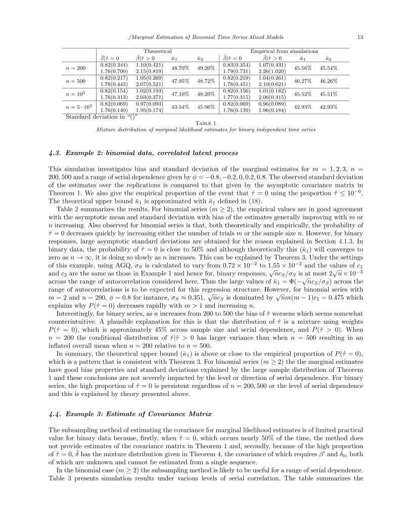
parentheses) of β conditional on τ = 0 and τ > 0 obtained from the simulations along with the theoreticalvalues of these obtained from (18), (16), and (22), (23) associated with Theorem 4.

Table 1 clearly demonstrates that for this data generating mechanism there is very high proportion ofreplicates for which τ = 0 and that this proportion does not decrease rapidly with sample size increasing.This is as predicted by theory and the theoretical values of κ1 and κ2 provide good approximations to κ1 andκ2. As explained above, this high proportion of zero estimates for τ , even for large sample sizes, is as expectedfor the regression structure used in this simulation. Note that κ1 ≤ κ2 and κ1 is closer to the probabilityof τ = 0. The estimations reverse the theoretical property that κ1 ≥ κ2. For binary data, P (τ = 0) andboth theoretical approximations, κ1 and κ2 decrease slowly and a very large sample is required to attainP (τ = 0) ≈ 0.

It is also clear from Table 1 that the empirical mean and standard deviation of β|τ = 0 and β|τ > 0show good agreement with the theoretical results predicted by Theorem 4. Overall, the theory we derive forP (τ = 0) and the use of a mixture distribution for β is quite accurate for all sample sizes, and with relativelylarge sample the mixture is a better representation. However, estimation of the corresponding distributionsin the mixture requires β0, τ0 and ψ0 and therefore cannot be implemented in practice.


Theoretical Empirical from simulations

β|τ = 0 β|τ > 0 κ1 κ2 β|τ = 0 β|τ > 0 κ1 κ2

n = 2000.82(0.344) 1.10(0.421)

48.70% 49.20%0.83(0.354) 1.07(0.431)

45.56% 45.54%1.76(0.700) 2.15(0.819) 1.79(0.731) 2.26(1.020)

n = 5000.82(0.217) 1.05(0.269)

47.95% 48.72%0.82(0.219) 1.04(0.261)

46.27% 46.26%1.76(0.443) 2.07(0.521) 1.78(0.451) 2.10(0.621)

n = 1030.82(0.154) 1.02(0.193)

47.10% 48.20%0.82(0.156) 1.01(0.182)

45.52% 45.51%1.76(0.313) 2.03(0.371) 1.77(0.315) 2.06(0.415)

n = 5 · 1030.82(0.069) 0.97(0.093)

43.54% 45.96%0.82(0.069) 0.96(0.089)

42.93% 42.93%1.76(0.140) 1.95(0.174) 1.76(0.139) 1.96(0.184)

Standard deviation in “()”Table 1

Mixture distribution of marginal likelihood estimates for binary independent time series

4.3. Example 2: binomial data, correlated latent process

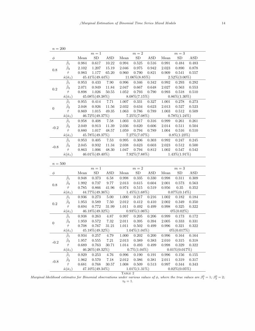
This simulation investigates bias and standard deviation of the marginal estimates for m = 1, 2, 3, n =200, 500 and a range of serial dependence given by φ = −0.8,−0.2, 0, 0.2, 0.8. The observed standard deviationof the estimates over the replications is compared to that given by the asymptotic covariance matrix inTheorem 1. We also give the empirical proportion of the event that τ = 0 using the proportion τ ≤ 10−6.The theoretical upper bound κ1 is approximated with κ1 defined in (18).

Table 2 summarizes the results. For binomial series (m ≥ 2), the empirical values are in good agreementwith the asymptotic mean and standard deviation with bias of the estimates generally improving with m orn increasing. Also observed for binomial series is that, both theoretically and empirically, the probability ofτ = 0 decreases quickly by increasing either the number of trials m or the sample size n. However, for binaryresponses, large asymptotic standard deviations are obtained for the reason explained in Section 4.1.3. Inbinary data, the probability of τ = 0 is close to 50% and although theoretically this (κ1) will converges tozero as n→∞, it is doing so slowly as n increases. This can be explained by Theorem 3. Under the settingsof this example, using AGQ, σS is calculated to vary from 0.72 × 10−2 to 1.55 × 10−2 and the values of c1and c2 are the same as those in Example 1 and hence for, binary responses,

√ncS/σS is at most 2

√n× 10−3

across the range of autocorrelation considered here. Thus the large values of κ1 = Φ(−√ncS/σS) across the

range of autocorrelations is to be expected for this regression structure. However, for binomial series withm = 2 and n = 200, φ = 0.8 for instance, σS ≈ 0.351,

√ncS is dominated by

√nm(m− 1)c1 = 0.475 which

explains why P (τ = 0) decreases rapidly with m > 1 and increasing n.Interestingly, for binary series, as n increases from 200 to 500 the bias of τ worsens which seems somewhat

counterintuitive. A plausible explanation for this is that the distribution of τ is a mixture using weightsP (τ = 0), which is approximately 45% across sample size and serial dependence, and P (τ > 0). Whenn = 200 the conditional distribution of τ |τ > 0 has larger variance than when n = 500 resulting in aninflated overall mean when n = 200 relative to n = 500.

In summary, the theoretical upper bound (κ1) is above or close to the empirical proportion of P (τ = 0),which is a pattern that is consistent with Theorem 3. For binomial series (m ≥ 2) the the marginal estimateshave good bias properties and standard deviations explained by the large sample distribution of Theorem1 and these conclusions are not severely impacted by the level or direction of serial dependence. For binaryseries, the high proportion of τ = 0 is persistent regardless of n = 200, 500 or the level of serial dependenceand this is explained by theory presented above.

4.4. Example 3: Estimate of Covariance Matrix

The subsampling method of estimating the covariance for marginal likelihood estimates is of limited practicalvalue for binary data because, firstly, when τ = 0, which occurs nearly 50% of the time, the method doesnot provide estimates of the covariance matrix in Theorem 1 and, secondly, because of the high proportionof τ = 0, δ has the mixture distribution given in Theorem 4, the covariance of which requires β′ and δ0, bothof which are unknown and cannot be estimated from a single sequence.

In the binomial case (m ≥ 2) the subsampling method is likely to be useful for a range of serial dependence.Table 3 presents simulation results under various levels of serial correlation. The table summarizes the


n = 200

m = 1 m = 2 m = 3φ Mean SD ASD Mean SD ASD Mean SD ASD

0.8

β1 0.984 0.617 10.22 0.994 0.525 0.516 0.991 0.484 0.483

β2 2.102 1.207 15.19 2.046 0.975 0.942 2.023 0.890 0.878τ 0.983 1.177 65.20 0.960 0.790 0.821 0.909 0.541 0.557

κ(κ1) 45.41%(49.44%) 11.06%(8.85%) 2.52%(3.00%)

0.2

β1 0.953 0.433 7.90 0.996 0.346 0.342 0.992 0.293 0.292

β2 2.071 0.949 11.84 2.047 0.667 0.648 2.027 0.563 0.553τ 0.898 1.026 50.55 1.052 0.793 0.790 0.993 0.518 0.510

κ(κ1) 45.08%(49.38%) 8.08%(7.15%) 0.86%(1.30%)

0

β1 0.955 0.414 7.71 1.007 0.331 0.327 1.001 0.278 0.273

β2 2.048 0.926 11.56 2.032 0.634 0.623 2.013 0.527 0.523τ 0.869 1.015 49.35 1.063 0.786 0.789 1.003 0.512 0.509

κ(κ1) 46.72%(49.37%) 7.25%(7.08%) 0.78%(1.24%)

-0.2

β1 0.958 0.408 7.58 1.003 0.317 0.316 0.999 0.261 0.261

β2 2.049 0.913 11.39 2.036 0.620 0.606 2.014 0.511 0.504τ 0.880 1.017 48.57 1.059 0.794 0.789 1.004 0.516 0.510

κ(κ1) 45.78%(49.37%) 7.27%(7.07%) 0.8%(1.23%)

-0.8

β1 0.953 0.405 7.53 0.995 0.306 0.303 0.992 0.247 0.245

β2 2.045 0.932 11.34 2.038 0.623 0.603 2.023 0.512 0.500τ 0.863 1.006 48.30 1.047 0.794 0.812 1.002 0.547 0.542

κ(κ1) 46.01%(49.40%) 7.92%(7.88%) 1.43%(1.91%)

n = 500

m = 1 m = 2 m = 3φ Mean SD ASD Mean SD ASD Mean SD ASD

0.8

β1 0.948 0.373 6.58 0.998 0.335 0.330 0.998 0.311 0.309

β2 1.992 0.737 9.77 2.013 0.615 0.604 2.001 0.573 0.563τ 0.785 0.866 41.96 0.974 0.515 0.519 0.956 0.35 0.352

κ(κ1) 44.77%(49.36%) 1.45%(1.68%) 0.07%(0.14%)

0.2

β1 0.936 0.273 5.00 1.000 0.217 0.216 1.002 0.182 0.184

β2 1.953 0.589 7.50 2.012 0.412 0.410 2.002 0.349 0.350τ 0.694 0.772 31.99 1.011 0.492 0.499 0.998 0.325 0.322

κ(κ1) 46.18%(49.32%) 0.93%(1.06%) 0%(0.02%)

0

β1 0.938 0.263 4.87 0.997 0.205 0.206 0.999 0.173 0.172

β2 1.959 0.572 7.32 2.011 0.395 0.394 2.005 0.333 0.331τ 0.708 0.767 31.21 1.011 0.502 0.499 0.996 0.321 0.322

κ(κ1) 45.18%(49.32%) 1.04%(1.04%) 0%(0.017%)

-0.2

β1 0.934 0.257 4.79 1.000 0.202 0.200 0.996 0.164 0.164

β2 1.957 0.555 7.21 2.013 0.389 0.383 2.010 0.315 0.318τ 0.689 0.763 30.71 1.014 0.493 0.499 0.998 0.329 0.322

κ(κ1) 46.26%(49.32%) 0.7%(1.04%) 0.01%(0.017%)

-0.8

β1 0.929 0.253 4.76 0.996 0.190 0.191 0.996 0.156 0.155

β2 1.962 0.570 7.18 2.012 0.386 0.381 2.011 0.319 0.317τ 0.681 0.768 30.57 1.008 0.509 0.513 0.997 0.344 0.343

κ(κ1) 47.10%(49.34%) 1.01%(1.31%) 0.02%(0.05%)Table 2

Marginal likelihood estimates for Binomial observations under various values of φ, where the true values are β01 = 1; β0

2 = 2;τ0 = 1.


m = 2, n = 200ASD SD kn = 5 kn = 11 kn = 23 kn = 46

φ = 0.8β1 0.515 0.525 0.392 0.406 0.387 0.325

β2 0.942 0.975 0.734 0.755 0.719 0.606τ 0.821 0.790 0.824 0.811 0.784 0.733

φ = 0.2β1 0.342 0.346 0.333 0.316 0.284 0.235

β2 0.648 0.667 0.637 0.605 0.545 0.447τ 0.790 0.793 0.829 0.814 0.786 0.729

φ = −0.2β1 0.316 0.322 0.313 0.296 0.265 0.221

β2 0.606 0.616 0.604 0.570 0.511 0.420τ 0.789 0.785 0.831 0.816 0.786 0.729

φ = −0.8β1 0.303 0.305 0.300 0.283 0.255 0.214

β2 0.603 0.619 0.592 0.562 0.508 0.419τ 0.812 0.796 0.842 0.834 0.808 0.750

m = 2, n = 500ASD SD kn = 7 kn = 14 kn = 28 kn = 56

φ = 0.8β1 0.330 0.330 0.261 0.275 0.271 0.242

β2 0.604 0.607 0.487 0.510 0.501 0.451τ 0.519 0.507 0.506 0.501 0.490 0.469

φ = 0.2β1 0.216 0.217 0.210 0.204 0.192 0.169

β2 0.410 0.418 0.400 0.388 0.364 0.321τ 0.499 0.493 0.503 0.497 0.486 0.465

φ = −0.2β1 0.199 0.199 0.197 0.190 0.179 0.159

β2 0.383 0.387 0.378 0.365 0.343 0.303τ 0.499 0.503 0.505 0.500 0.490 0.469

φ = −0.8β1 0.191 0.191 0.188 0.182 0.171 0.152

β2 0.381 0.387 0.372 0.361 0.340 0.302τ 0.513 0.513 0.514 0.511 0.502 0.481

Table 3Subsampling estimates for standard deviation of GLMM estimation, kn = C[n1/3], C = 1, 2, 4, 8.

estimates of standard deviation for δ using the subsampling method described in Section 2.2. The column“ASD” contains the asymptotic standard deviation calculated with the covariance matrix in Theorem 1and column “SD” contains empirical standard deviation. The table shows the subsampling estimates ofstandard deviations are of the same magnitude of theoretical standard deviations even for moderate samplesize n = 200 but are biased downwards and increasingly so as C increases. Values of C = 1, 2 provide theleast biased estimates for the standard errors for both sample sizes. Downwards bias is greater for largepositive values of φ as might be expected.

5. Alternative to Marginal Likelihood Estimation

We close with a discussion of the alternative approach for binary time series regression modelling proposedby Wu and Cui (2014). Their modified GLM (MGLM) method replaces exp(xT

ntβ)/(1 + exp(xTntβ)) in the

GLM log-likelihood 4 with a function π(xTntβ) representing the marginal mean to arrive at the objective

function

l2(β) =

n∑t=1

[yt log π(xT

ntβ) + (1− yt) log(1− π(xT

ntβ))] , π(xT

ntβ) =

∫ex

Tntβ+αt

1 + exTntβ+αt

g(αt)dα. (31)

The MGLM estimate β2 is found by iterating two steps starting with the GLM estimate of β: step 1, estimatethe curve of π(u) =

∫eu+α/(1 + eu+α)g(α)dα non-parametrically on u ∈ R; step 2, maximize l2 with respect

to β, based on the estimate of π(u) obtained in the first step. Steps 1 and 2 are repeated and the iterationstops when the maximum value of l2 is reached and the last update of β is then regarded as the MGLMestimator. Implementation details are provided in Wu and Cui (2014).

In defining their method Wu and Cui (2014) do not require that π(u) =∫eu+α/(1 + eu+α)g(α)dα for any

distribution g of the latent process. Hence it is not required that π(u) be non-negative and strictly increasing

in u. However, their main theorem concerning consistency and asympototic normality of β2 is stated in terms


of this latent process specification. For such specifications, application of their non-parameteric method forestimating π(u) requires additional constraints which are not currently implemented. For example, taking thefirst derivative with respect to u, gives π(u) =

∫eu+α/(1+eu+α)2g(α)dα ≤ π(u)(1−π(u)) so π(u) ∈ [0, 0.25]

by application of Jensen’s inequality. When applied to the Cambridge-Oxford Boat Race time series thenon-parameteric estimate of π(u) is not monotonic and produces marginal estimates, at values of u between

the gaps in the observed values of xTntβ2, which are zero and therefore not useful for prediction at new values

of the linear predictor.Although not implemented in the R-code of Wu and Cui (2014), this constraint as well as that of mono-

tonicity can be enforced in the nonparametric estimation of p(u) using an alternative local linearization tothat used in Wu and Cui (2014). For example, with constraints of monotonicity and π(u) ∈ [0, 0.25], different

estimates β1 = 0.2093, β2 = 0.1899 (compared to β1 = 0.237, β2 = 0.168 in Wu and Cui (2014)) are observedfor the model for the Cambridge-Oxford boat race series that they analyse. In this example, the marginallikelihood estimates give τ = 0 and hence β degenerates to GLM estimate which differs from that of Wuand Cui (2014). Somehow the marginal method (with or without monotonocity contraints) is avoiding thedegeneracy issue that arises with the marginal estimation method proposed in this paper. This needs to befurther understood.

While MGLM is computationally much more intensive than using standard GLMM methods for obtainingthe marginal estimates it appears to avoid degeneracy but for reasons that are not fully understood at thisstage. Additionally, it is not clear the extent to which MGLM with or without the proper constraints impliedby a latent process specification avoids the high proportion of degenerate estimates observed with GLMMfor binary data. Additionally the extent to which MGLM reproduces the correct curve for the marginalprobabilities π(u) when the true data generating mechanism is defined in terms of a latent process (parameterdriven specification) has not been investigated. The extent to which the MGLM estimate of π(u) differs fromthe curve defined by a latent process specification might form the basis for a non-parametric test of thedistribution of the latent process – when αt is not Gaussian, the true curve of π(u) is not the same with

that evaluated under GLMM fits, and we may end up into different results for the estimates of β2 and β.

6. Discussion

To overcome the inconsistency of GLM estimates of the regression parameters in parameter driven binomialmodels time series models we have proposed use of the marginal likelihood estimation, which can be easilyconducted using the generalized linear mixing model fitting packages. We have shown that the estimatesof regression parameters and latent process variation obtained from this method are consistent and asymp-totically normal even if the observations are serially dependent. The distribution of the marginal estimatesis required for a score test of serial dependence in the latent process something which we will report onelsewhere. The asymptotic results and proofs thereof have assumed that the latent process is Gaussian whichhas helped streamline the presentation. This is not required for all results except for Lemma 2 (asymptoticidentifiability for the binary case) which relies directly on the normal distribution. The proofs can be readilymodified provided we assume that the moment generating function mαt(u) of αt is finite for all u <

√(d2)

where τ < d2 defines the parameter space.The structure of the model considered here is such that the theoretical results apply to other response

distributions such as the Poisson and negative binomial with very little change in the proofs of theorems.GLM estimation in these cases is consistent and asymptotically normal regardless of serial dependence inthe latent process. The same will be true of the use of marginal estimation with the advantage that thelatent process variability is also estimated. While we have not yet shown this, we expect that for these otherresponse distributions the use of marginal estimation will lead to more efficient estimates of the regressionparameters.

For all response distributions and for moderate sample sizes the marginal estimation method can result ina non-zero probability of τ = 0. As we have observed in simulations, and explained via theoretical asymptoticarguments, this is particularly problematical for binary responses with very high probabilities being observed(and expected from theory) for ‘pile-up’ probability for τ . We have observed that for binomial data (m > 1)the ‘pile-up’ probability quickly decreases to zero and, as a result of this observation, we anticipate that thisprobability will not typically be large for Poisson and negative Binomial responses.


For binary data we have developed a useful upper bound approximation to this probability and subse-quently proposed an improved mixture distribution for β in finite samples. These theoretical derivations arewell supported by simulations presented. While this mixture distribution cannot be used based on a singletime series none-the-less it provided useful insights into the sampling properties of marginal estimation forbinary time series. Additionally the derivations suggest that regression models in which xTβ varies overan interval over which the inverse logit function is approximately linear will be particularly prone to the‘pile-up’ problem and this persists even when there is strong serial dependence. Practitioners should applythe marginal likelihood method with caution in such situations.

7. Acknowledgements

We thank Dr Wu and Dr Cui for providing us with the R-code for their application of the MGLM methodto the Boat Race Data reported in Wu and Cui (2014).

8. Appendix: A

Proof of Lemma 1. We consider the deterministic regressors only in this proof but the same arguments canbe extended to stochastic regressors. Now M is the largest value of m for which kM > 0, so Q(δ) = Q(δ0) ifand only if ∫ 1

0

M∑j=0

π0(j, h(u))(log π(j, h(u))− log π0(j, h(u))

)du = 0

Since the integrand is non-positive the integrand can be zero if and only if the integrand is zero almosteverywhere. Hence, for a contradiction, assume ∃δ 6= δ0 such that

M∑j=0

π0(j, h(u))(log π(j, h(u))− log π0(j, h(u))

)= 0, ∀u ∈ [0, 1].

and this can only happen if π0(j, h(u)) = π(j, h(u)) for all j = 0, . . . ,M . Since

π(j, h(u)) =

∫ (M

j

)b(h(u)Tβ +

√τz)j(1− b(h(u)Tβ +

√τz))M−jφ(z)dz

it is straightforward to show, by iterating from j = 0, . . . ,M , that π0(j, h(u)) = π(j, h(u)) for all j = 0, . . . ,Mis equivalent to ∫

b(h(u)Tβ +√τz)jφ(z)dz =

∫b(h(u)Tβ0 +

√τ0z)

jφ(z)dz, j = 1, . . . ,M, (32)

for any u ∈ [0, 1]We next show that the only way this can hold is if δ = δ0. Fix u and denote a = h(u)Tβ, a0 = h(u)Tβ0

and σ =√τ ,

dj(a, σ) = E[b(a+ σz)j

]− E

[b(a0 + σ0z)

j], j = 1, . . . ,M.

where expectation is with respect to the density φ(·). Hence (32) is equivalent to so that d1(a0, σ0) =d2(a0, σ0) = · · · = dM (a0, σ0) = 0. Assume η0 = (a0, σ0), if there exists η 6= η0 such that (32) holds, thenthere is ‖η∗ − η0‖ ≤ ‖η − η0‖ such that

d1(a, σ)d2(a, σ)

...dM (a, σ)

=

E[b(η∗)0b(η∗)

]E[b(η∗)0b(η∗)z

]2E[b(η∗)1b(η∗)

]2E[b(η∗)1b(η∗)z

]...

...

ME[b(η∗)M−1b(η∗)

]ME

[b(η∗)M−1b(η∗)z

]

(v1

v2

)= J(η∗)

(v1

v2

)(33)


where v1 = a− a0 and v2 = σ− σ0 cannot be zero at the same time when η 6= η0, which is equivalent to thematrix J(η∗) being of full rank. But J(η∗) is not of full rank if and only if the ratios of the second columnto the first column are the same for all j = 1, . . . ,M . However, we now show that this ratio increases as jincreases. Since b(·) and b(·) are non-negative functions we can define probability densities

gj(z) =b(a∗ + σ∗z)j−1b(a∗ + σ∗z)φ(z)∫b(a∗ + σ∗z)j−1b(a∗ + σ∗z)φ(z)dz

, j = 1, . . . ,M

so that

E[b(η∗)j b(η∗)z

]E[b(η∗)j b(η∗)

] =

∫zb(a∗ + σ∗z)g(z)dz∫b(a∗ + σ∗z)g(z)dz

=Egj (zb(a∗ + σ∗z))

Egj (b(a∗ + σ∗z))

where Egj () denotes expectation with respect to gj . But since b(a∗ + σ∗z) is an increasing function of z, z

and b(a∗ + σ∗z) are positively correlated. Therefore,

Egj (z) < Egj (zb(a∗ + σ∗z))/Egj (b(a∗ + σ∗z))

it follows that

E[b(η∗)j−1b(η∗)z

]E[b(η∗)j−1b(η∗)

] <E[b(η∗)j b(η∗)z

]E[b(η∗)j b(η∗)

] , j = 1, . . . ,M.

Then when (32) holds, (33) has a unique solution of (0, 0) for (v1, v2), which contradicts to the assumptionthat η 6= η0. Thus (32) holds if and only if η = η0, which implies a = a0 and σ = σ0. By Condition 3, we canconclude that a = a0 for all u implies β = β0. Therefore Condition 5 holds for M ≥ 2.

Proof of Lemma 2. This proof considers the Fourier transform method used in Wang and Louis (2003).Assume ∃δ 6= δ0 such that ∀x ∈ X,

π0(1) =

∫b(xTβ0 + σ0z)φ(z)dz =

∫b(xTβ + σz)φ(z)dz = π(1), σ =

√τ .

For connected X, the first derivative with respect to x of both sides are also the same, that is∫b(xTβ0 + σ0z)φ(z)dz · β0 =

∫b(xTβ + σz)φ(z)dz · β (34)

which implies there exists a constant c1 > 0 such that c1 = βk/β0,k for k = 1, . . . , r, with η = xTβ,c2 = σ/σ0 > 0, (34) can be rewritten as convolutions∫

g(u)h(η − u)du = c1

∫g(u)h(c1η − c2u)du; h(x) =

ex

(1 + ex)2, g(x) =

1

σ0

√2π

exp(− x2

2σ20

).

let G(s) be the Fourier transform of the normal density g(·), H(s) be the Fourier transform of the logisticdensity h(·), using the fact that the Fourier transform of the convolution is the product of Fourier transformof each function,

G(s)H(s) =

∫ (∫c1φ(u)h(c1η − c2u)du

)e−iηsdη

= c1

∫φ(u)

(∫h(c1η − c2u)e−iηsdη

)du

= c1

∫φ(u)

(∫h(c1η − c2u)e−i(c1η−c2u)(s/c1)d(c1η − c2u)

)|c1|−1e−iu(c2s/c1)du

=

∫φ(u)e−iu(c2s/c1)duH(s/c1) =

c1|c1|

G(c2s/c1)H(s/c1), c1 > 0.


it follows that G(s)H(s) = G(c2s/c1)H(s/c1), ∀s ∈ R. The Fourier transform for the mean zero normaldistribution is G(s) = exp(− 1

2σ20s

2), and the Fourier transform for the logistic distribution is H(s) =2πs/(eπs − e−πs), thus for any s 6= 0,

exp(−1

2σ2

0s2)

1

sinh(πs)= exp(−1

2σ2

0s2

(c2c1

)2

)1

c1 sinh(πs/c1)

for any fixed c1 6= 1, c2 can be expressed as a function of s and this function is not a constant over s, whichcontradicts to the definition of c2. Hence the equality holds if and only if c1 = 1 and c2 = 1.

9. Appendix: B

Proof of Theorem 1. This proof is presented in three steps: first, we show, for any δ ∈ Θ, that E(Qn(δ))defined in (9) converges to Q(δ) defined in (10) and (11) under Condition 2a and 2b respectively; second,

that Qn(δ)− E(Qn(δ))a.s→ 0 where Qn(δ) is defined in (8) from which, using compactness of the parameter

space, it follows that δa.s.→ δ0; third, that

√n(δ − δ0)

d→ N(0,Ω−11,1Ω1,2Ω−1

1,1).

Proof that E(Qn(δ))a.s.→ Q(δ): Use Jensen’s inequality multiple times we have

−mt∑j=0

π0t (j) lnπt(j) ≤

mt∑j=0

π0t (j)

mt∑j=0

(− lnπt(j))

= −mt∑j=0

lnπt(j)

≤−mt∑j=0

(j(xTt β)−mt(ln 2 + max(xTt β + τ/2, 0)) + c(j)

)≤

mt∑j=0

[mt(ln 2 + τ/2) +mt|xTt β| − c(j)

]< mt(1 +mt)

(ln 2 + τ/2 + |xTt β|

)(35)

then conditional on mt and xt,∑mt

j=0 π0t (j) lnπt(j) is bounded for all t and δ. Under Condition 2a, the

regressor xnt := h(t/n) is nonrandom as is the marginal density πnt. Then the strong law of large numbersfor mixing processes (McLeish, 1975) applied to mt gives

limn→∞

1

n

n∑t=1

mt∑j=0

π0nt(j) log πnt(j) = lim

n→∞

1

n

n∑t=1

E

mt∑j=0

π0nt(j) log πnt(j)

= Q(δ)

defined in (10). For Condition 2b the ergodic properties of the stationary processes mt and Xt can be usedto establish

limn→∞

1

n

n∑t=1

mt∑j=0

π0t (j) log πt(j) = lim

n→∞

M∑m=1

nmn

1

nm

∑t:mt=m

m∑j=0

π0t (j) log πt(j)

= Q(δ)

defined in (11).

Consistency : We write (8) as Qn(δ) = n−1∑∞t=1 qt(δ) where qt(δ) = log f(yt|xnt, δ). By Blais, MacGibbon

and Roy (2000, Proposition 1), qt(δ) is strongly mixing for any δ ∈ Θ. To apply the strong law of largenumbers for mixing process in McLeish (1975) we need to show that ∃λ ≥ 0 such that

∞∑t=1

‖qt(δ)− Eqt(δ)‖22+λ/t2 <∞

where ‖ · ‖p denotes the Lp norm. By Minkowski’s inequality and Holder’s inequality,

‖qt(δ)− Eqt(δ)‖2+λ ≤ 2 ‖qt(δ)‖2+λ


using similar derivations as used in (35), |qt(δ)| ≤ |−mt|xTntβ|+c(yt)−mt(ln 2+τ/2)| where mt is bounded. Itsuffices to establish

∑∞t=1 ‖qt(δ)‖22+λ/t

2 <∞ if∑∞t=1 |xT

ntβ|2/t2 <∞. Under Condition 2a, xTntβ is bounded

for any given β;∑∞t=1 1/t2 < 2, therefore the result follows. Under Condition 2b, we have E‖x‖2 <∞, given

any β, for all ε > 0,

P

(n∑t=1

|xT

t β|2/t2 ≥ K

)≤ (2/K)E|xTβ|2 ≤ ε, if K ≥ 2E|xTβ|2/ε.

Then n−1∑nt=1 [qt(δ)− Eqt(δ)]

a.s.→ 0 for any δ ∈ Θ. Together with the first part of the proof given above

we now have Qn(δ)a.s→ Q(δ). Since Θ is a compact set, and Qn(δ) is a continuous function of δ for all n, by

Gallant and White (1988, Theorem 3.3), δ := arg maxΘ

Qn(δ)a.s.→ δ0.

Asymptotic Normality : Using a Taylor expansion,

√n(δ − δ0) = −

(1

n

n∑t=1

lt(δ∗)

)−11√n

n∑t=1

lt(δ0), δ∗a.s.→ δ0

the asymptotic normality of√n(δ − δ0) can be obtained if

− 1

n

n∑t=1

lt(δ∗)

p→ Ω1,1 and1√n

n∑t=1

lt(δ0)d→ N(0,Ω1,2).

Conditional on mt and xnt, lt(δ) is strongly mixing. Then by Chebyshev’s inequality and Ibragimovand Yu (1971, Theorem 17.2.3), ∃ε > 0 such that

1

n

n∑t=1

lt(δ)−1

n

n∑t=1

E(lt(δ))p→ 0, ‖δ − δ0‖ ≤ ε

Since δ∗a.s.→ δ0, and the continuity of lt(·) with respect to δ, n−1

∑nt=1 lt(δ

∗) − n−1∑nt=1 lt(δ0)

a.s.→ 0,

and n−1∑nt=1 lt(δ0) − n−1

∑nt=1E(lt(δ0))

a.s.→ 0. Now E(lt(δ0)) = E(lt(δ0)lTt (δ0)), and hence it follows that

n−1∑t=1 lt(δ

∗)p→ Ω1,1.

Next we show that Ω1,1 is positive definite. Let s = (s1, s2) be an (r + 1) dimensional constant vector,

without lose of generality, sTs = 1. Define qt(δ0) = sT lt(δ0), note det(Ω1,1) ≥ 0 and det(Ω1,1) = 0 only ifE(q2t (δ0)|mt, xnt

)= 0 for all t. Then under Condition 3, Ω1,1 is positive definite. The limit, Ω1,1, under

Condition 2a is given in (28). For stationary regressors such limit can be easily obtained using ergodictheorem.

Next we show Ω1,2 exists. Note

Ω1,2 = limn→∞

Var

(1√n

n∑t=1

qt(δ0)

)=

n−1∑h=0

(1

n

n−h∑t=1

Cov(qt(δ0), qt+h(δ0))

)+

n−1∑h=1

(1

n

n∑t=h+1

Cov(qt(δ0), qt−h(δ0))

)

then Ω1,2 exists if

limn→∞

n−1∑h=0

(1

n

n−h∑t=1

|Cov(qt(δ0), qt+h(δ0))|

)<∞, lim

n→∞

n−1∑h=1

(1

n

n∑t=h+1

|Cov(qt(δ0), qt−h(δ0))|

)<∞.

Since the qt(δ0) is strong mixing, by Theorem 17.3.2 in Ibragimov and Yu (1971),

n−1∑h=0

(1

n

n−h∑t=1

|Cov(qt(δ0), qt+h(δ0))|

)≤ 2

n−1∑h=0

ν(h)λ/(2+λ)Wh <∞,


where

Wh = limn→∞

1

n

n−h∑t=1

[4 + 3(ctc

1+λt+h + c1+λ

t ct+h)], ct ≥ ‖qt(δ0)‖2+λ

Such ct exists, for example, take λ = 2, use Cauchy-Schwarz’s inequality,

E(|qt(δ0)|4|mt, xnt

)≤ E

∫f(yt|xnt, zt, δ0)φ(zt)

((yt −mtb(W0,t))(s

T

1xnt + s2zt))4

dz · f−1(yt|xnt, δ0)

= E

[mtb(W0,t)(1 + (3mt − 6)b(W0,t))(s

T

1xnt + s2zt)4|mt, xnt

]Then by the application of CLT for mixing process in Theorem 3.2, Davidson (1992) we will have

n−1/2∑nt=1 lt(δ0)

d→ N(0,Ω1,2).

Proof of Theorem 2. Following the proof of Davis, Dunsmuir and Wang (2000) and Wu and Cui (2014), letu =√n(β − β′) (note here we centre on β′ and not the true value β0 as was done in these references). Then

maximizing

ln(β) =

n∑t=1

[yt(xT

ntβ)−mtb(xT

ntβ) + c(yt)]

over β is equivalent to minimizing gn(u) over u where gn(u) := −ln(β′+u/√n)+ln(β′). Let u = arg min lim

n→∞gn(u).

Write gn(u) := Bn(u)−An(u) where

Bn(u) :=

n∑t=1

mt

(b(xTt β

′ + xTt u/√n)− b(xTt β′)− b(xTt β′)xTt u/

√n)

and

An(u) := uT1√n

n∑t=1

(yt −mtb(xTt β′))xt = uTUn.

Using similar procedures as in the proof of Theorem 1. in Wu and Cui (2014) it is straightforward to show

Bn(u)→ 1

2uTΩ1u

and

E(eis

TUn

)= exp

[−1

2sTΩ2s

].

for each u. Since gn(u) is a convex function of u and un minimizes gn(u), then an application of the functional

limit theory gives und→ u, where u = arg min lim

n→∞gn(u). In conclusion,

gn(u)d→ g(u) =

1

2uTΩ1u− uTN(0,Ω2)

on the space C(Rr), and und→ u, where u ∼ N(0,Ω−1

1 Ω2Ω−11 ).

Proof of Theorem 3. Since S1,n(β), a linear function of U1,n and U2,n, to show that√n(S1,n(β)− E(S1,n(β′))

)is normally distributed it is sufficient to show that the the joint distribution of (U1,n, U2,n) is multivariatenormal. As defined in (21),

U1,n := S1,n(β′)− E (S1,n(β′)) =1√n

n∑t=1

e2t,β′ − Ee2

t,β′ ; U2,n := Ω−11

1√n

n∑t=1

et,β′xnt =1√n

n∑t=1

et,β′cnt

where cnt = Ω−11 xnt, defines a sequence of non-random vectors.

Let Unt = (U1,nt, U2,nt) be the joint vector at time t, then each dimension of Unt is uniformly bounded,strongly mixing and E(Unt) = 0. We need to prove that a1U1,n+aT2 U2,n has normal distribution for arbitrary


constant vector a = (a1, a2) where aTa = 1 without loss of generality. By the SLLN for mixing process inMcLeish (1975), there exists a limiting matrix ΩU such that

Var(

n∑t=1

aTUnt) =

n−1∑h=0

(n−h∑t=1

aTCov(Unt, Un,t+h)a

)+

n−1∑h=1

(n∑

t=1+h

aTCov(Unt, Un,t−h)a

)→ aTΩUa.

Then conditions of the CLT of Davidson (1992) are satisfied, and we have∑nt=1 Unt

d→ N(0,ΩU ).

Proof of Theorem 4. This proof follows Moran (1971). δ0 is the true value of the parameters, δ′ = (β′, 0) is

the limit of parameters that maximize (7) for fixed τ = 0; δ is the maximum likelihood estimators of (7).

Consider first the distribution of δ if τ > 0. Since the unconditional joint distribution of β and τ ismultivariate normal with N(0,Ω−1

1,1Ω1,2Ω−11,1) – see proof of Theorem 1, hence F2(c, δ0), the distribution of

√n(β − β0)|τ > 0 is skew normal based on N(0,Ω−1

1,1Ω1,2Ω−11,1).

When τ = 0, use a Taylor expansion to the first derivatives around δ′, then

√n(β − β′) =

(− 1

n

n∑t=1

lt(δ′)

)−11√n

n∑t=1

∂lt(δ′)

∂β+ op(1),

conditional on n−1/2∑nt=1 ∂lt(δ

′)/∂τ < 0. As n→∞,

1√n

n∑t=1

∂lt(δ′)

∂δ=

( 1√n

∑nt=1 et,β′xnt

12√n

∑nt=1

[e2t,β′ −mtb(x

Tt β′)]) d→ N(

(0

E(S1,n(β′))/2

),

(Ω2 KS/2

KTS /2 VS/4

))

References

Blais, M., MacGibbon, B. and Roy, R. (2000). Limit theorems for regression models of time series ofcounts. Statistics & probability letters 46 161–168.

Cox, D. R. (1981). Statistical analysis of time series: some recent developments. Scandinavian Journal ofStatistics 8 93–115.

Davidson, J. (1992). A central limit theorem for globally nonstationary near-epoch dependent functions ofmixing processes. Econometric theory 5 313–329.

Davis, R. A., Dunsmuir, W. T. and Wang, Y. (2000). On autocorrelation in a Poisson regression model.Biometrika 87 491–505.

Davis, R. A. and Dunsmuir, W. T. M. (2015). State Space Models for Count Time Series. CRC MONO-GRAPHS.

Davis, R. A. and Wu, R. (2009). A negative binomial model for time series of counts. Biometrika 96735–749.

Dunsmuir, W. T. M., Tran, C. and Weatherburn, D. (2008). Assessing the Impact of MandatoryDNA Testing of Prison Inmates in NSW on Clearance, Charge and Conviction Rates for Selected CrimeCategories. NSW Bureau of Crime Statistics and Research.

Gallant, A. R. and White, H. (1988). A unified theory of estimation and inference for nonlinear dynamicmodels. Basil Blackwell New York.

Gupta, A. K., Gonzalez-Farıas, G. and Domınguez-Molina, J. A. (2004). A multivariate skew normaldistribution. Journal of Multivariate Analysis 89 181–190.

Heagerty, P. J. and Lumley, T. (2000). Window subsampling of estimating functions with applicationto regression models. Journal of the American Statistical Association 95 197–211.

Ibragimov, I. A. and Yu, V. L. (1971). Independent and stationary sequences of random variables. Wolters-Noordhoff.

McLeish, D. L. (1975). A maximal inequality and dependent strong laws. The Annals of probability 3829–839.


Moran, P. A. (1971). Maximum likelihood estimation in non-standard conditions. Mathematical Proceedingsof the Cambridge Philosophical Society 70 441–450.

Neuhaus, J. M., Kalbfleisch, J. D. and Hauck, W. W. (1991). A comparison of cluster-specificand population-averaged approaches for analyzing correlated binary data. International Statistical Re-view/Revue Internationale de Statistique 59 25–35.

Wang, Z. and Louis, T. A. (2003). Matching conditional and marginal shapes in binary random interceptmodels using a bridge distribution function. Biometrika 90 765–775.

Wu, R. (2012). On variance estimation in a negative binomial time series regression model. Journal ofMultivariate Analysis 112 145–155.

Wu, R. and Cui, Y. (2014). A PARAMETER-DRIVEN LOGIT REGRESSION MODEL FOR BINARYTIME SERIES. Journal of Time Series Analysis 35 462-477.

Marginal Estimation of Parameter Driven Binomial Time ... · Marginal Estimation of Parameter...

Documents

Transcript of Marginal Estimation of Parameter Driven Binomial Time ... · Marginal Estimation of Parameter...