Marginal cost curves for water footprint reduction in irrigated...

Hydrol. Earth Syst. Sci., 21, 3507–3524, 2017https://doi.org/10.5194/hess-21-3507-2017© Author(s) 2017. This work is distributed underthe Creative Commons Attribution 3.0 License.

Marginal cost curves for water footprint reduction in irrigatedagriculture: guiding a cost-effective reduction of crop waterconsumption to a permit or benchmark levelAbebe D. Chukalla1, Maarten S. Krol1, and Arjen Y. Hoekstra1,2

1Twente Water Centre, University of Twente, Enschede, the Netherlands2Institute of Water Policy, Lee Kuan Yew School of Public Policy, National University of Singapore, Singapore

Correspondence to: Abebe D. Chukalla ([email protected])

Received: 4 February 2017 – Discussion started: 17 February 2017Revised: 24 May 2017 – Accepted: 8 June 2017 – Published: 13 July 2017

Abstract. Reducing the water footprint (WF) of the pro-cess of growing irrigated crops is an indispensable elementin water management, particularly in water-scarce areas. Toachieve this, information on marginal cost curves (MCCs)that rank management packages according to their cost-effectiveness to reduce the WF need to support the deci-sion making. MCCs enable the estimation of the cost as-sociated with a certain WF reduction target, e.g. towards agiven WF permit (expressed in m3 ha−1 per season) or to acertain WF benchmark (expressed in m3 t−1 of crop). Thispaper aims to develop MCCs for WF reduction for a rangeof selected cases. AquaCrop, a soil-water-balance and crop-growth model, is used to estimate the effect of different man-agement packages on evapotranspiration and crop yield andthus the WF of crop production. A management packageis defined as a specific combination of management prac-tices: irrigation technique (furrow, sprinkler, drip or subsur-face drip); irrigation strategy (full or deficit irrigation); andmulching practice (no, organic or synthetic mulching). Theannual average cost for each management package is esti-mated as the annualized capital cost plus the annual costs ofmaintenance and operations (i.e. costs of water, energy andlabour). Different cases are considered, including three crops(maize, tomato and potato); four types of environment (hu-mid in UK, sub-humid in Italy, semi-arid in Spain and aridin Israel); three hydrologic years (wet, normal and dry years)and three soil types (loam, silty clay loam and sandy loam).For each crop, alternative WF reduction pathways were de-veloped, after which the most cost-effective pathway was se-lected to develop the MCC for WF reduction. When aiming

at WF reduction one can best improve the irrigation strat-egy first, next the mulching practice and finally the irriga-tion technique. Moving from a full to deficit irrigation strat-egy is found to be a no-regret measure: it reduces the WFby reducing water consumption at negligible yield reductionwhile reducing the cost for irrigation water and the associ-ated costs for energy and labour. Next, moving from no toorganic mulching has a high cost-effectiveness, reducing theWF significantly at low cost. Finally, changing from sprin-kler or furrow to drip or subsurface drip irrigation reducesthe WF, but at a significant cost.

1 Introduction

In many places, water use for irrigation is a major factor con-tributing to water scarcity (Rosegrant et al., 2002; Mekonnenand Hoekstra, 2016), which will be worsened by increasingdemands for food and biofuels (Ercin and Hoekstra, 2014). Inmany regions, climate change will aggravate water scarcityby affecting the spatial patterns of precipitation and evapora-tion (Vörösmarty et al., 2000; Fischer et al., 2007). Reduc-ing the water footprint (WF) of crop production, i.e. the con-sumption of rainwater (green WF) and irrigation water (blueWF) per unit of crop, is a means of increasing water pro-ductivity and reducing water scarcity (Hoekstra, 2017). Toensure that the blue WF in a catchment remains within themaximum sustainable level given the water renewal rate inthe catchment, Hoekstra (2014) proposes to establish a blueWF cap per catchment and issue no more blue WF permits to

Published by Copernicus Publications on behalf of the European Geosciences Union.

3508 A. D. Chukalla et al.: Marginal cost curves for water footprint reduction

individual users than fit within the cap. This would urge wa-ter users to reduce their blue WF to a level that is sustainablewithin the catchment. Additionally, in order to increase wa-ter use efficiency, Hoekstra (2014) proposes water footprintbenchmarks for specific processes and products as a refer-ence for what is a reasonable level of water consumption perunit of production. This would provide an incentive for wa-ter users to reduce their WF per unit of product down to acertain reasonable reference level. The reduction of the WFin irrigated agriculture to the benchmark level relates to im-proving the physical water use efficiency or increasing wa-ter productivity (Molden et al., 2010), thus relieving waterscarcity (Mekonnen and Hoekstra, 2014; Zhuo et al., 2016;Zwart et al., 2010). WF reduction in irrigated crop produc-tion can be achieved through a range of measures, includ-ing a change in mulching practice or in irrigation techniqueor strategy. Chukalla et al. (2015) studied the effectivenessof different combinations of irrigation technique, irrigationstrategy and mulching practice in terms of WF reduction. Noresearch thus far has been carried out regarding the costs ofWF reduction. A relevant question though is how much itcosts to reduce the WF of crop production to a certain tar-get such as a WF benchmark for the water consumption pertonne of crop or a WF permit for the water consumption perarea.

The current study makes a first effort in response to thisquestion by analysing the cost-effectiveness of various mea-sures in irrigated crop production in terms of cost per unit ofWF reduction and introducing marginal cost curves (MCC)for WF reduction. An MCC for WF reduction is a tool thatpresents how different measures can be applied subsequentlyin order to achieve an increasing amount of WF reduc-tion, whereby measures are ordered according to their cost-effectiveness (WF reduction achieved per cost unit). Everynew measure introduced brings an additional (i.e. marginal)cost and an incremental (marginal) reduction of the WF.There are model-driven and expert-based approaches to de-velop an MCC. The two approaches have been applied ex-tensively to assess the costs of carbon footprint reductionin various studies, focusing on various sectors and regions.Enkvist et al. (2007) show cost curves for reducing green-house gas emissions for different regions in the world. Lewisand Gomer (2008) develop an MCC for reducing greenhousegas emissions of all sectors in Australia, and MacLeod etal. (2010) develop an MCC for the agricultural sector in theUK. A detailed method to derive MCCs for the most econom-ically efficient reductions in greenhouse gas emissions in theagricultural sector is presented by Bockel et al. (2012). Theweaknesses and strengths intrinsic to different methods ofderiving MCCs of greenhouse gas reduction are reviewed indifferent papers (Kesicki, 2010; Kesicki and Strachan, 2011;Kesicki and Ekins, 2012).

The application of MCCs in the water sector is just start-ing. Addams et al. (2009) apply MCCs for closing the gap be-tween water supply and demand in irrigated agriculture, par-

ticularly focussing on the reduction of irrigation water with-drawal. Khan et al. (2009) discuss two possible pathways toincrease water productivity and energy use efficiency in foodproduction. This work, however, does not explicitly specifythe measures and their cost-effectiveness, which would in-form the unit cost of improving water and energy use ef-ficiency. Other studies, like Gonzalez-Alvarez et al. (2006)and Samarawickrema and Kulshreshtha (2009), focus on themarginal cost of water but do not develop MCCs. The firststudy mentioned studies how farmers would respond if themarginal cost of irrigation water is changed; the second studyassesses the marginal value of irrigation water in the produc-tion of alternative crops in order to allocate the water basedon the highest marginal value. In the area of WF reductionspecifically, MCCs have been developed only once, not inthe agricultural sector however, but in a case for some fac-tories in different industrial sectors using the expert-basedapproach (Tata-Group, 2013). The current paper pioneers bydeveloping and applying a model-driven MCC in the area ofWF reduction in irrigated agriculture. It thus fills a gap of theexisting literature on WF reduction, which generally lacksthe practical and economic component: what are the subse-quent steps and associated costs to achieve increasing levelsof water footprint reduction.

The objective of this study is to develop alternative WF re-duction pathways and the MCC for WF reduction in irrigatedcrop production. We do so for a number of crops and environ-ments. We apply the AquaCrop model, a soil-water-balanceand crop-growth model that can be used to estimate the WFof crop production under different management practices,linked with a cost model that calculates annual costs relatedto different management practices, to systematically assessboth WF and costs of 20 management packages. Four casestudy areas are considered: Rothamsted in the UK, Bolognain Italy, Badajoz in Spain, and Eilat in Israel. Based on theoutcomes we construct WF reduction pathways and marginalcost curves. Finally, we illustrate the application of the MCCfor WF reduction with a selected case with a certain WF re-duction target given a situation where the actual WF needs tobe reduced given a cut in the WF permit.

2 Method and data

2.1 Research set-up

We consider the production of three crops (maize, tomato andpotato) under four environments (humid, sub-humid, semi-arid and arid), three hydrologic years (wet, normal and dryyear) and three soil types (loam, silty clay loam and sandyloam). We distinguish 20 management packages, wherebyeach management package is defined as a specific combina-tion of management practices: irrigation technique (furrow,sprinkler, drip or subsurface drip); irrigation strategy (full or

Hydrol. Earth Syst. Sci., 21, 3507–3524, 2017 www.hydrol-earth-syst-sci.net/21/3507/2017/

A. D. Chukalla et al.: Marginal cost curves for water footprint reduction 3509

Management packages

Irrigation technique

Drip

Subsurface drip

Furrow

Sprinkler

Irrigation strategy

Deficit irrigation

Full irrigation

Mulching practice

Synthetic

Organic

No mulching

Water footprint

AquaCrop & global WF

accounting standard

Average annual cost

Cost per management package

(capital plus operation and

maintenance cost)

Marginal cost curves for WF reduction

WF reduction pathways

2

4

3

1

Figure 1. Flow chart for developing marginal cost curves for cropproduction.

deficit irrigation); and mulching practice (no, organic or syn-thetic mulching).

We develop the marginal cost curves (MCCs) for WF re-duction in irrigated crop production in four steps (Fig. 1).First, we calculate the WF of growing a crop under the dif-ferent environmental conditions and management packagesusing the AquaCrop model (Raes et al., 2013). Second, thetotal annual average costs for the management packages werecalculated. Third, we constructed plausible WF reductionpathways starting from different initial situations. A WF re-duction pathway shows a sequence of complementary mea-sures, stepwise moving from an initial management packageto management packages with lower WFs. Finally, MCCs forWF reduction were deduced based on reduction potential andcost-effectiveness of the individual steps. This approach doesnot aim to represent a cost–benefit analysis from an agro-economic perspective. Reduced costs through water savingsare included, but monetary benefits to the farmer through in-creased yield or product quality are not included. In this way,the approach fully focusses on costs to save water. Yield in-creases do have a direct impact on final results by reducingthe WF per unit of product.

2.2 Management packages

Each management package is a combination of a specificirrigation technique, irrigation strategy and mulching prac-tice. We consider four irrigation techniques, two irrigationstrategies and three mulching practices. From the 24 pos-sible combinations, we exclude four unlikely combinations,namely the combinations of furrow and sprinkler techniqueswith synthetic mulching (with either full or deficit irrigation),leaving 20 management packages considered in this study.

The four irrigation techniques differ considerably in thewetted area generated by irrigation (Ali, 2011). In the anal-ysis, default values from the AquaCrop model are taken for

the wetted area for each irrigation, as recommended by Raeset al. (2013). For furrow irrigation, an 80 % wetting percent-age is assumed to be representative for a narrow bed furrow,from the indicative range of 60 to 100 %. For the sprinkler,drip and subsurface drip irrigation techniques, wetted areasby irrigation of 100, 30 and 0 %, respectively, are used.

Two irrigation strategies are analysed: full and deficit irri-gation. Irrigation requires two principal decisions of schedul-ing: the volume of water to be irrigated and timing of irriga-tion. Full irrigation is an irrigation strategy in which the fullevaporative demand is met; this strategy aims at maximizingyield. Its irrigation schedule is simulated through automaticgeneration of the required irrigation to avoid any water stress.The irrigation schedule in the no water stress condition iscrop-dependent: the soil moisture is refilled to field capacitywhen 20, 36 and 30 % of readily available water (RAW) ofthe soil is depleted for maize, potato and tomato, respectively(FAO, 2012). This scheduling results in a high irrigation fre-quency, which is impractical in the case of furrow and sprin-kler irrigation. To circumvent such unrealistic simulation forthe case of furrow and sprinkler irrigation, the simulated ir-rigation depths are aggregated in such a way that a time gapof a week is maintained between two irrigation events.

Deficit irrigation (DI) is the application of water belowthe evapotranspiration requirements (Fereres and Soriano,2007) by limiting water applications particularly during lessdrought-sensitive growth stages (English, 1990). The deficitstrategy is established by reducing the irrigation supply be-low the full irrigation requirement. We extensively tested var-ious deficit irrigation strategies that fall under two broad cat-egories: (1) regulated deficit irrigation, where a non-uniformwater deficit level is applied during the different phenologicalstages; and (2) sustained deficit irrigation, where the waterdeficit is managed to be uniform during the whole crop cy-cle. In the analysis of simulations, the specific deficit strategythat is optimal according to the model experiments and foryield reduction not exceeding 2 % is used. AquaCrop simu-lates water stress responses triggered by soil moisture deple-tion using three thresholds for a restraint on canopy expan-sion, stomatal closure and senescence acceleration (Stedutoet al., 2009b).

Mulching is the process of covering the soil surface arounda plant to create good-natured conditions for its growth (La-mont et al., 1993; Lamont, 2005). Mulching has various pur-poses: reduce soil evaporation, control weed incidence andits associated water transpiration, reduce soil compaction,enhance nutrient management and incorporate additional nu-trients (McCraw and Motes, 1991; Shaxson and Barber,2003; Mulumba and Lal, 2008). The AquaCrop model sim-ulates the effect of mulching on evaporation and representseffects of soil organic matter through soil hydraulic proper-ties influencing the soil water balance. Soil evaporation undermulching practices is simulated by scaling the evaporationwith a factor that is described by two variables (Raes et al.,2013): the fraction of soil surface covered by mulch (from

www.hydrol-earth-syst-sci.net/21/3507/2017/ Hydrol. Earth Syst. Sci., 21, 3507–3524, 2017


0 to 100 %); and a parameter representing mulch material(fm). The correction factor (CF) for the effect of mulchingon evaporation is calculated as

CF= (1− fm×mc) (1)

with mc being the fraction of the soil covered by mulch. Weassume a mulching factor fm of 1.0 for synthetic mulching,0.5 for organic mulching and zero for no mulching as sug-gested by Raes et al. (2013). Further we take a mulch coverof 100 % for organic and 80 % for synthetic materials, againas suggested in the AquaCrop reference manual (Raes et al.,2013).

2.3 Calculation of water footprint per managementpackage

The water footprint (WF) of crop production is a volumetricmeasure of freshwater use for growing a crop, distinguish-ing between the green WF (consumption of rainwater), blueWF (consumption of irrigation water or consumption of soilmoisture from capillary rise) and grey WF (water pollution)(Hoekstra et al., 2011). The green and blue WF, which are thefocus in the current study, are together called the consump-tive WF. To allow for a comprehensive and systematic assess-ment of consumptive WF, this study employs the AquaCropmodel to estimate green and blue evapotranspiration (ET)and crop yield (Y ) to calculate blue and green WF of cropproduction.

We use the plug-in version of AquaCrop 4.1 (Steduto etal., 2009a; Raes et al., 2011) and determine the crop grow-ing period based on growing degree days. The AquaCropmodel simulates the soil water balance in the root zone witha daily time step over the crop growing period (Raes et al.,2012). The fluxes into and from the root zone are runoff, in-filtration, evapotranspiration, drainage and capillary rise. Thegreen and blue fractions in total ET are calculated based onthe green to blue water ratio in the soil moisture, which inturn is kept track of over time by accounting for how muchgreen and blue water enter the soil moisture, following theaccounting procedure as reported in Chukalla et al. (2015).

AquaCrop simulates actual ET and biomass growth basedon the type of crop grown (with specific crop parameters),the soil type, climate data such as precipitation and referenceET (ETo), and given water and field management practices.We estimate ETo based on FAO’s ETo calculator that uses thePenman–Monteith equation (Allen et al., 1998). The modelseparates daily ET into crop transpiration (productive) andsoil evaporation (non-productive).

Evaporation (E) is calculated by multiplying the referenceET (ETo) by factors that consider the fraction of the soil sur-face not covered by canopy, and water stress. When the soilsurface is soaked by rainfall or irrigation or when soil mois-ture is beyond a level called readily evaporable water (RAW),the evaporation rate is fully determined by the energy avail-able for soil evaporation (Ritchie, 1972). When soil moisture

drops below RAW, the so-called falling rate stage, the evap-oration is determined by the available energy and hydraulicproperties of the soil field. Experimental studies in differentenvironments have shown that the AquaCrop model reason-ably simulates evaporation, transpiration and thus ET (Af-shar and Neshat, 2013; Saad et al., 2014).

The crop growth engine of AquaCrop estimates thebiomass by multiplying water productivity and transpirationand computes yield by multiplying biomass by the harvestindex. Water productivity is assumed to respond to atmo-spheric evaporative demand and atmospheric CO2 concen-tration (Steduto et al., 2009a).

We express the WF of crop production in two ways. Thegreen and blue WFs per unit of land (m3 ha−1) are calculatedas the green and blue evapotranspiration over the growingperiod of a crop. The green and blue WFs per unit of produc-tion (m3 t−1) are calculated by dividing green or blue evapo-transpiration over the growing period of a crop (m3 ha−1) bythe crop yield (t ha−1). The crop yield in terms of dry mat-ter per hectare as obtained from the AquaCrop calculationsis translated into a fresh crop yield (the marketable yield)per hectare. The dry matter fractions of marketable yield fortomato, potato and maize are estimated to be 7, 25 and 100 %,respectively (Steduto et al., 2012). The variability of greenand blue WF is presented by calculating the standard devia-tion of the estimated WFs across different environments, hy-drologic years and soil types.

2.4 Estimation of annual cost per management package

The overall cost of a management package includes initialcapital or investment costs (IC), operation costs (OC), andmaintenance costs (MC). Investment costs include costs ofinstalling a new irrigation system and/or buying plastics forsynthetic mulching. Operation costs refer to costs for irri-gation water, energy and labour. Maintenance costs includelabour and material costs. Both OC and MC are expressed asannual cost (USD ha−1 yr−1).

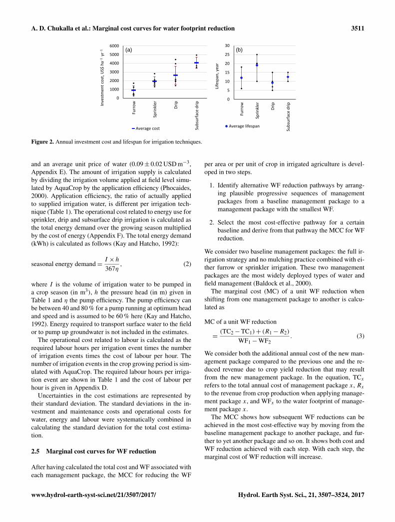
Figure 2 shows the average annual investment cost of ir-rigation techniques and their lifespan. The data are derivedfrom different sources as specified in Appendices A and B.Investment costs that were reported as one-time instalmentcosts were converted to equivalent annual costs based ona 5 % interest rate and the lifespan of the techniques. Theaverage annual maintenance cost per irrigation technique –including costs for labour and material – is assumed to beequivalent to 2 % of the annualized investment costs (Kayand Hatcho, 1992).

The average annual investment costs of 1112 USD ha−1

for synthetic mulching are based on the sources as speci-fied in Appendix C. We further assume average operationand maintenance costs of 140 USD ha−1 yr−1 for syntheticmulching and 200 USD ha−1 yr−1 for organic mulching.

The operational cost related to the use of irrigation wa-ter is calculated from the amount of irrigation water applied



0

1000

2000

3000

4000

5000

6000

Furr

ow

Spri

nkl

er

Dri

p

Sub

surf

ace

dri

p

Inve

stm

ent

cost

, US$

ha

yr

-1

Average cost

0

5

10

15

20

25

30

Furr

ow

Spri

nkl

er

Dri

p

Sub

surf

ace

dri

p

Life

span

, yea

r

Average lifespan

(a) (b)

-1

Figure 2. Annual investment cost and lifespan for irrigation techniques.

and an average unit price of water (0.09± 0.02 USD m−3,Appendix E). The amount of irrigation supply is calculatedby dividing the irrigation volume applied at field level simu-lated by AquaCrop by the application efficiency (Phocaides,2000). Application efficiency, the ratio of actually appliedto supplied irrigation water, is different per irrigation tech-nique (Table 1). The operational cost related to energy use forsprinkler, drip and subsurface drip irrigation is calculated asthe total energy demand over the growing season multipliedby the cost of energy (Appendix F). The total energy demand(kWh) is calculated as follows (Kay and Hatcho, 1992):

seasonal energy demand=I ×h

367η, (2)

where I is the volume of irrigation water to be pumped ina crop season (in m3), h the pressure head (in m) given inTable 1 and η the pump efficiency. The pump efficiency canbe between 40 and 80 % for a pump running at optimum headand speed and is assumed to be 60 % here (Kay and Hatcho,1992). Energy required to transport surface water to the fieldor to pump up groundwater is not included in the estimates.

The operational cost related to labour is calculated as therequired labour hours per irrigation event times the numberof irrigation events times the cost of labour per hour. Thenumber of irrigation events in the crop growing period is sim-ulated with AquaCrop. The required labour hours per irriga-tion event are shown in Table 1 and the cost of labour perhour is given in Appendix D.

Uncertainties in the cost estimations are represented bytheir standard deviation. The standard deviations in the in-vestment and maintenance costs and operational costs forwater, energy and labour were systematically combined incalculating the standard deviation for the total cost estima-tion.

2.5 Marginal cost curves for WF reduction

After having calculated the total cost and WF associated witheach management package, the MCC for reducing the WF

per area or per unit of crop in irrigated agriculture is devel-oped in two steps.

1. Identify alternative WF reduction pathways by arrang-ing plausible progressive sequences of managementpackages from a baseline management package to amanagement package with the smallest WF.

2. Select the most cost-effective pathway for a certainbaseline and derive from that pathway the MCC for WFreduction.

We consider two baseline management packages: the full ir-rigation strategy and no mulching practice combined with ei-ther furrow or sprinkler irrigation. These two managementpackages are the most widely deployed types of water andfield management (Baldock et al., 2000).

The marginal cost (MC) of a unit WF reduction whenshifting from one management package to another is calcu-lated as

MC of a unit WF reduction

=(TC2−TC1)+ (R1−R2)

WF1−WF2. (3)

We consider both the additional annual cost of the new man-agement package compared to the previous one and the re-duced revenue due to crop yield reduction that may resultfrom the new management package. In the equation, TCxrefers to the total annual cost of management package x, Rxto the revenue from crop production when applying manage-ment package x, and WFx to the water footprint of manage-ment package x.

The MCC shows how subsequent WF reductions can beachieved in the most cost-effective way by moving from thebaseline management package to another package, and fur-ther to yet another package and so on. It shows both cost andWF reduction achieved with each step. With each step, themarginal cost of WF reduction will increase.



Table 1. The application efficiency, labour intensity and pressure head required per irrigation technique.

Irrigation technique Application efficiency Labour intensity Pressure head(%) (h ha−1 per irrigation event) (m)

Source Brouwer et al. (1989), Kay and Hatcho (1992) Reich et al. (2009) andKay and Hatcho (1992), Phocaides (2000)

Phocaides (2000)

Furrow 60 2.0–4.0 0Sprinkler 75 1.5–3.0 25Drip 90 0.2–0.5 13.6Subsurface drip 90 0.2–0.6 13.6

2.6 Data

The WFs were calculated for four locations (UK, Italy,Spain and Israel), three hydrological years (wet, normaland dry years) and three soil types (loam, silty clay loam,and sandy loam). The input data on climate and soilwere collected from four sites: Rothamsted in the UK(52.26◦ N, 0.64◦ E; 69 m above mean sea level), Bologna inItaly (44.57◦ N, 11.53◦ E; 19 m a.m.s.l.), Badajoz in Spain(38.88◦ N, −6.83◦ E; 185 m a.m.s.l.) and Eilat in Israel(29.33◦ N, 34.57◦ E; 12 m a.m.s.l.). These sites are character-ized by humid, sub-humid, semi-arid, and arid environments,respectively. Daily observed climatic data (rainfall, minimumand maximum temperature) were extracted from the Euro-pean Climate Assessment and Dataset (ECAD) (Klein Tanket al., 2002). Wet, normal and dry years were selected from20 years of daily rainfall data (observed data from the period1993 to 2012). Daily ETo values for the wet, normal and dryyears were derived using FAO’s ETo calculator (Raes, 2012).Soil texture data, which are extracted with a resolution of1× 1 km2 from the European Soil Database (Hannam et al.,2009), are used to identify the soil type based on the soiltexture triangle calculator (Saxton et al., 1986). The physi-cal characteristics of the soils are taken from the default pa-rameters in AquaCrop. For crop parameters, by and large wetake the default values as represented in AquaCrop. However,the rooting depth for maize at the Bologna site is restrictedto a maximum of 0.7 m to account for the actual local con-dition of a shallow groundwater table (average 1.5 m). Themain components of the average annual cost per managementpackage have been collected from the literature. We use cropprices per crop and per country averaged over 5 years (2010–2015) from FAOSTAT (2017); the costs for water, labour andenergy are averaged over data for Spain, Italy and the UK, i.e.from three of the four countries studied here. An overview ofthe costs and their sources is presented in Appendices A to F.In presenting the WF estimates per management package, weshow averages over the different cases as well as the range ofoutcomes for the cases (different environments, hydrologicyears and soil types). To develop the MCCs, we use the av-erages.

3 Results

3.1 Water footprint and cost per management package

Figures 3 and 4 show the WF per area and WF per unit ofcrop, and the annual average costs corresponding to 20 man-agement packages.

For each combination of a certain mulching practice andirrigation strategy, the consumptive WF and the blue WFin particular decrease when we move from sprinkler to fur-row to drip and further to subsurface drip irrigation. Undera given irrigation strategy and mulching practice, the WFin m3 ha−1 in the case of subsurface drip irrigation is 6.2–13.3 % smaller than in the case of sprinkler irrigation. Theannual average cost always increases from furrow to sprin-kler and further to drip and subsurface drip irrigation. Undera given mulching practice and irrigation strategy, the cost inthe case of furrow irrigation is 58–63 % smaller than in thecase of subsurface drip irrigation. The cost of furrow irriga-tion is small particularly because of the relatively low invest-ment cost, which is higher for sprinkler and even higher fordrip and subsurface drip irrigation. The operational costs, bycontrast, are higher for sprinkler and furrow than for drip orsubsurface drip irrigation, because of the higher water con-sumption and thus cost for sprinkler and furrow. Sprinklerhas the highest operational cost because it requires a highpressure head to distribute the water (hence the higher en-ergy cost).

Under a given irrigation technique and mulching practice,DI always results in a slightly smaller WF in m3 ha−1 (inthe range of 1.6–5.7 %) and lower cost (in the range of 4–14 %) as compared to full irrigation (FI). The decrease incost is due to the decrease in water and pumping energy.The WF of crop production always decreases in a stepwiseway when going from no mulching to organic mulching andthen to synthetic mulching, while the costs increase along themove. This cost increase relates to the growing material andlabour costs when applying mulching (most with syntheticmulching), but the net cost increase is tempered by the factthat less water and pumping energy will be required.



0

1000

2000

3000

4000

5000

6000

7000

8000

Spri

nkl

er

Furr

ow

Dri

p

Sub

surf

ace

dri

p

Spri

nkl

er

Furr

ow

Dri

p

Sub

surf

ace

dri

p

Spri

nkl

er

Furr

ow

Dri

p

Sub

surf

ace

dri

p

Spri

nkl

er

Furr

ow

Dri

p

Sub

surf

ace

dri

p

Dri

p

Sub

surf

ace

dri

p

Dri

p

Sub

surf

ace

dri

p

0

1000

2000

3000

4000

5000

6000

7000

8000

WF in m3 ha-1

Cost, US$ ha-1

Green WF Blue WF Investment cost Water cost Energy cost Labour cost

No mulching

Full irrigation

No mulching

Deficit irrigation

Organic mulching

Full irrigation

Organic mulching

Deficit irrigation

Synthetic mulching

Full Deficit

Figure 3. Average WF per area (m3 ha−1) for maize production and average annual costs associated with 20 management packages. Thewhiskers around WF estimates indicate the range of outcomes for the different cases (different environments, hydrologic years and soiltypes). The whiskers around cost estimates indicate uncertainties in the costs. WF estimates are split up into blue and green components;costs are split up into investment, water, energy and labour costs.

0

1000

2000

3000

4000

5000

6000

7000

8000

Spri

nkl

er

Furr

ow

Dri

p

Sub

surf

ace

dri

p

Spri

nkl

er

Furr

ow

Dri

p

Sub

surf

ace

dri

p

Spri

nkl

er

Furr

ow

Dri

p

Sub

surf

ace

dri

p

Spri

nkl

er

Furr

ow

Dri

p

Sub

surf

ace

dri

p

Dri

p

Sub

surf

ace

dri

p

Dri

p

Sub

surf

ace

dri

p

0

100

200

300

400

500

600

700

800

WFm3 t-1

Green WF Blue WF Investment cost Water cost Energy cost Labour cost

CostU$ ha-1

No mulching

Full irrigation

No mulching

Deficit irrigation

Organic mulching

Full irrigation

Organic mulching

Deficit irrigation

Synthetic mulching

Full Deficit

Figure 4. Average WF per product unit (m3 t−1) for maize production and average annual costs associated with 20 management packages.The whiskers around the WF estimates indicate the range of outcomes for the different cases (different environments, hydrologic years andsoil types). The whiskers around cost estimates indicate uncertainties in the costs.

Figure 5 shows the scatter plot of the 20 managementpackages, the abscissa and ordinate of each point represent-ing the average annual cost and average WF, respectively, ofa particular management package. In this graph, the blue ar-row indicates the direction of decreasing WF and costs. Thepoints or management packages connected by the blue lineare jointly called the Pareto optimal front or non-dominatedPareto optimal solutions. Moving from one to another man-agement package on the line means that WF will decrease

while cost increases, or vice versa, which implies that alongthis line there will always be a trade-off between the twovariables. “Best solutions” may be identified using the MCCwhen policy goals are specified, for instance a certain WF re-duction target in m3 t−1 or m3 ha−1 is to be achieved, or thelargest WF reduction is to be achieved with a given limitedbudget. Each management package that is not on the line canbe improved in terms of reducing cost or reducing WF at no



cost for the other variable, or even WF reduction and costdecrease can be achieved simultaneously.

3.2 Water footprint reduction pathways

In developing a new irrigation scheme or renovating an ex-isting one in a water-scarce area, it would be rational to im-plement one of the management packages from the Paretooptimal set if the goal is to arrive at a cost-effective mini-mization of the WF of crop production. In an existing farm,where the management package is not in the Pareto optimalset, there can be alternative pathways towards reducing theWF. This involves a stepwise adoption of complementarymeasures that eventually leads to a management package inthe Pareto optimal set.

Figure 6 shows alternative WF reduction pathways fromthe two most common baseline management packages: fullirrigation and no mulching with either furrow or sprinkler ir-rigation. The figure shows four WF reduction pathways fromthe baseline with furrow irrigation and two pathways fromthe baseline with sprinkler irrigation. In all pathways, theWF of crop production is continually reduced by changingone thing at a time, i.e. either the irrigation technique, the ir-rigation strategy or the mulching practice. In some cases, astep may be accompanied by a cost reduction, but in the endmost steps imply a cost increase. Logically, all pathways endat a point at the Pareto optimal front.

3.3 Marginal cost curves for WF reduction

Not all alternative WF reduction pathways from a specificbaseline are equally cost-effective. In both cases it makesmuch sense to move from full to deficit irrigation first, be-cause that reduces the WF and cost at the same time. Next,it is best to move from no to organic mulching because thecost-effectiveness of this measure is very high, which can bemeasured in the graph (Fig. 6) as the steep slope (high WF re-duction per dollar). Finally, the most cost-effective measure,in both cases, is to move towards drip irrigation in combina-tion with synthetic mulching. One could also move to drip ir-rigation and stay with organic mulching, which is also Paretooptimal; the cost of this will be less, but the WF reductionwill be less as well. However, moving to drip irrigation incombination with synthetic mulching is more cost-effective(higher WF reduction per dollar) than moving to drip irriga-tion while staying with organic mulching.

For both baseline management packages, we have drawnthe MCCs in Figs. 7 and 8 for the case of maize. The curvesare shown both for reducing the WF per area (Figs. 7a and8a) and the WF per unit of product (Figs. 7b and 8b). Fromthese curves, we can read the most cost-effective measuresthat can subsequently be implemented. For each step we canread in the graph what the associated marginal cost is andwhat the associated WF reduction is. In both cases, the firststep goes at a negative cost, i.e. a benefit, while the next steps

go at increasing marginal cost. Each step is shown in the formof a bar, with the height and width representing the cost perunit WF reduction and the WF reduction, respectively. Thearea under a bar represents the total cost of implementing themeasure.

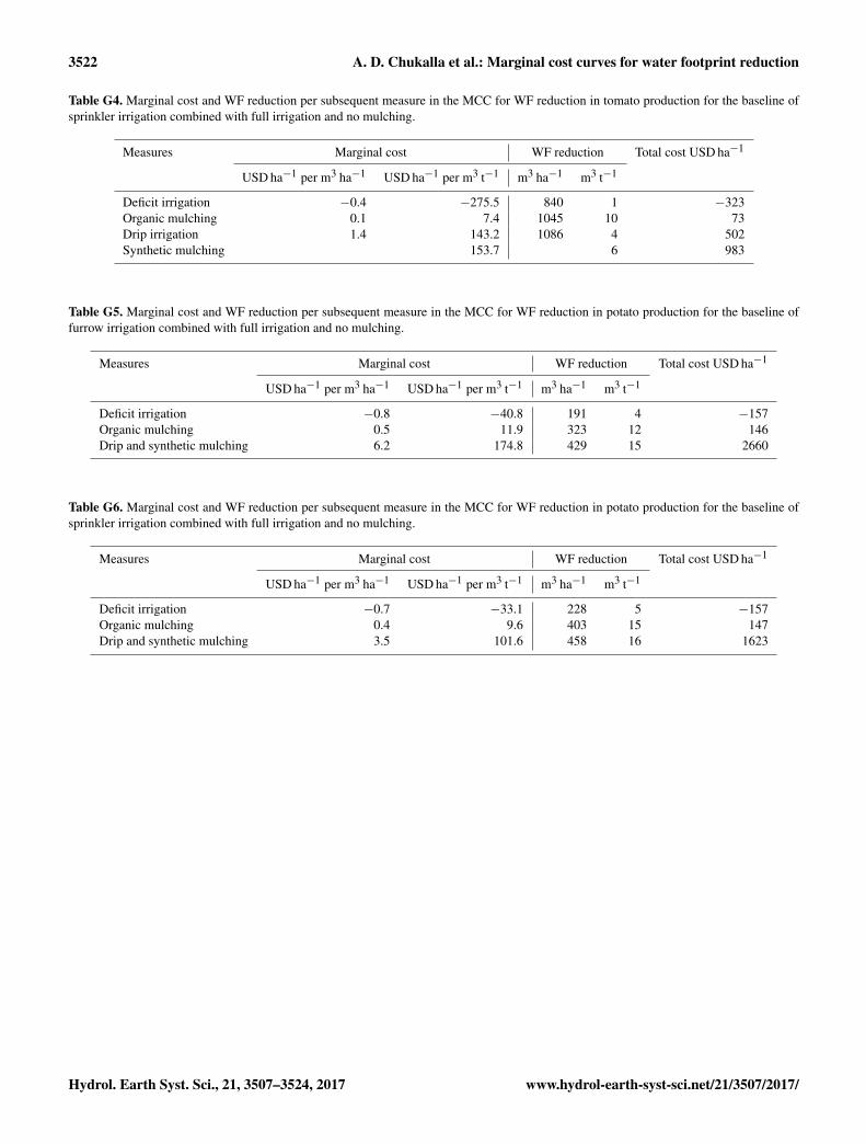
For tomato and potato we find similar results as for maize,as shown by the data presented in Appendix G.

3.4 Application of the marginal cost curve

In this section, we elaborate a practical application of anMCC for WF reduction, using a selected case with a certainWF reduction target given a situation where the actual WFneeds to be reduced given a cut in the WF permit. The futureintroduction of WF permits to water users or WF benchmarksfor products in water-scarce areas is likely if the sustain-able development goals (SGDs) are to be met, particularlySDG 6.4, which reads “by 2030, substantially increase water-use efficiency across all sectors and ensure sustainable with-drawals and supply of freshwater to address water scarcity,and substantially reduce the number of people suffering fromwater scarcity”. Here we will illustrate how an MCC for WFreduction can help in achieving a certain WF reduction goal.

An MCC for WF reduction – ranking measures accordingto their cost-effectiveness in reducing WF – can be used toestimate what measures can best be taken and what is the as-sociated total cost to achieve a certain WF reduction target.For farmers, it will not be attractive to go beyond the imple-mentation of those WF reduction measures that reduce costsas well, but from a catchment perspective further WF reduc-tion may be required. An MCC will show the societal costassociated with a certain WF reduction goal. Governments,food companies and investors can make use of this informa-tion to develop incentive schemes for farmers and/or invest-ment plans to implement the most cost-effective measures inorder to achieve a certain WF reduction in a catchment or ata given farm.

In a hypothetical example, the WF in the river basin ex-ceeds the maximum sustainable level. Agriculture in thebasin consists of irrigated maize production with a currentconsumptive WF on the farms of 6380 m3 ha−1. The farmsapply sprinkler and full irrigation and no mulching. In or-der to reduce water consumption in the basin to a sustainablelevel, the river basin authority proposes various measures in-cluding a regulation that prohibits land expansion for cropproduction and the introduction of a WF permit to the maizefarmers that allows them to use no more than 5200 m3 ha−1.This means they have to reduce the WF of maize produc-tion by 1180 m3 ha−1. Figure 9 shows how the MCC for WFreduction can help in this hypothetical example to identifywhat measures can best be taken to reduce the WF by therequired amount and what costs will be involved.

As shown in the figure, we best implement deficit irriga-tion first (providing a total benefit of 189 USD ha−1, whichis the net result of a USD 231 gain from saved water and



SP:FI:NM

FU:FI:NM

DR:FI:NM SD:FI:NM

SP:DI:NM

FU:DI:NM

DR:DI:NMSD:DI:NM

SP:FI:OM

FU:FI:OM

DR:FI:OMSD:FI:OM

SP:DI:OMFU:DI:OM

DR:DI:OM

SD:DI:OM

DR:FI:SMSD:FI:SM

DR:DI:SM SD:DI:SM

4000

4500

5000

5500

6000

6500

7000

1000 2000 3000 4000 5000 6000

WF,

m3

ha-1

yr-1

Cost, US$ ha-1 yr -1

FU - furrow FI - full irrigation NM - no mulching

SP - sprinkler DI - deficit irrigation OM - organic mulching

DR - frip SM - synthetic mulching

SD - subsurface drip

Figure 5. Pareto optimal front for WF and cost reduction in irrigated crop production. The dots represent the annual cost of maize productionand the WF per area for 20 management packages. The line connects the Pareto optimal management packages.

SP:FI:NM

FU:FI:NM

DR:FI:NMSD:FI:NM

SP:DI:NM

FU:DI:NM

DR:DI:NMSD:DI:NM

SP:FI:OMFU:FI:OM

DR:FI:OMSD:FI:OM

SP:DI:OM

FU:DI:OM

DR:DI:OM SD:DI:OM

DR:FI:SM SD:FI:SM

DR:DI:SMSD:DI:SM

4000

4500

5000

5500

6000

6500

7000

1000 2000 3000 4000 5000 6000

WF,

m3

ha-1

yr-1

Cost, U$ ha-1 yr -1

Fu - furrow FI - full irrigation NM - no mulching SP - sprinkler DI - deficit irrigation OM - organic mulching DR - drip SM - synthetic mulching SD - subsurface drip

Furrow Full irrigation No mulching

Sprinkler: full irrigation: no mulching

Figure 6. WF reduction pathways for maize from two baseline management packages: full irrigation and no mulching with either furrow orsprinkler irrigation.

a USD 42 loss from crop yield decline), followed by or-ganic mulching (with a total cost of 72 USD ha−1). Thethird and last step to finally achieve the required WF reduc-tion can be to implement drip irrigation combined with syn-thetic mulching on 25 % of the maize fields (at a total costof 366 USD ha−1). The other 75 % is then still with sprin-kler and organic mulching, but the combined result meetsthe target. Alternatively, because in this particular case thecost-effectiveness of moving to drip irrigation with organicmulching is close to the cost-effectiveness of moving to dripirrigation with synthetic mulching, one could move in thethird step in 100 % of the fields to drip irrigation with or-ganic mulching, which would result in a WF reduction of

1176 m3 ha−1. In order to meet the full target, a small per-centage of the total fields would need to implement syntheticmulching in addition.

4 Discussion

The current paper introduces the method for developingMCCs for WF reduction in irrigated agriculture, and showshow the MCCs can be applied to achieve a certain WF re-duction target, like reducing the WF to a certain WF permitlevel (in m3 ha−1) or WF benchmark level (in m3 t−1). Wateravailability per catchment is limited to runoff minus envi-



Co

st o

f W

F re

du

ctio

n, U

S$ h

a-1 p

er m

3t-1

Drip and synthetic mulching Organic

mulching

Deficit irrigation

Drip and synthetic mulching

Organic mulching

Deficit irrigation

Co

st o

f W

F re

du

ctio

n, U

S$ h

a-1 p

er m

3 h

a-1

WF reduction, m3 ha-1 WF reduction, m3 t-1

(a) (b)

Figure 7. Marginal cost curves for WF reduction for maize for the baseline of furrow irrigation combined with full irrigation and no mulching.(a) WF reduction per area. (b) WF reduction per unit of product.

Deficit irrigation

Co

st o

f W

F re

du

ctio

n, U

S$ h

a-1 p

er m

3 h

a-1

Co

st o

f W

F re

du

ctio

n, U

S$ h

a-1 p

er m

3t-1

WF reduction, m3 ha-1 WF reduction, m3 t-1

Organic mulching


Deficit irrigation

Organic mulching


(a) (b)

Figure 8. Marginal cost curve for WF reduction of maize for the baseline of sprinkler irrigation combined with full irrigation and nomulching. (a) WF reduction per area. (b) WF reduction per unit of product.

ronmental flow requirement (Hoekstra, 2014). When divid-ing the maximum amount of water available in a catchmentover the croplands that need irrigation, one finds a maximumvolume of water available per hectare of cropland. This couldbe translated in water allocation policy into a maximum WFpermit per hectare; this is just one way of promoting WFreduction in areas where that is needed. Another way is tocreate incentives to reduce the WF per unit of production toa certain benchmark level. Thus, the MCCs we develop canbe used for analysing a cost-effective WF reduction pathwaygiven either a target level for WF per hectare or a target levelfor WF per unit of crop.

By comparing the cost-effectiveness of measures in reduc-ing the WF of growing crops, we found that one can best im-prove first the irrigation strategy (moving from full to deficitirrigation), next the mulching practice (moving from no toorganic mulching) and finally the irrigation technique (fromfurrow or sprinkler irrigation to drip or subsurface drip ir-rigation). In our cost-effectiveness analysis, we did not in-clude the cost of bringing irrigation water from source tofield. The cost will be high when the source is a deep wa-ter well and/or far away, and low if irrigation water flows to a

field by gravitational force or by natural pressure, for exam-ple from an artesian aquifer or an elevated reservoir. Given acertain source and distance, the total cost to bring irrigationwater from source to field will depend on the volume of waterto be transported, which varies across the management pack-ages. We excluded this cost, because it does not affect thefinding from the study, as we will explain. The cost of sup-plying water will be highest for furrow irrigation (becausethis technique involves the largest irrigation water supply atfield level), followed by sprinkler and drip or subsurface dripirrigation. Furthermore, the water supply cost is higher forfull than for deficit irrigation. Finally, the water supply costis highest in the case of the no-mulching practice (whichrequires the highest irrigation water supply, because ET ishighest), followed by organic and synthetic mulching. Thewater supply cost for transporting the water to the field thusdecreases in the direction of decreasing WF, which impliesthat the order of changing management practices in order toreduce WFs in the most cost-effective way does not changeby including water supply costs in the equation. It implies,though, that we underestimated the cost savings associatedwith water supply to the field when reducing WFs.



Co

st o

f W

F re

du

ctio

n,

U$

ha-1

per

m3

ha-1

WF reduction, m3 ha-1

Deficit irrigation

Organic mulching

(Drip and synthetic mulching

1180 1180

WF reduction, m3 ha-1

Synthetic mulching

Drip

Organic mulching

Deficit irrigation

(a) (b)

Figure 9. Application of the MCC in an example where the WF of maize production needs to be reduced. The baseline is sprinkler, fullirrigation and no mulching with a WF of 6380 m3 ha−1. This needs to be reduced by 1180 m3 ha−1 in order to meet a given local WF permit.(a) In the third step, drip irrigation combined with synthetic mulching is implemented on 25 % of the area. (b) In the third step, drip irrigation(maintaining organic mulching) is implemented on 100 % of the area, while in a fourth step synthetic mulching is implemented on 0.5 % ofthe area.

The derivation of plausible WF reduction pathways re-quires insight into the agronomic plausibility of successiveimplementation measures in the field. Our findings suggestfirst moving from full to deficit irrigation, then from no to or-ganic mulching, and finally from furrow or sprinkler irriga-tion to drip or subsurface drip irrigation, which is a plausiblepathway of changing management practices. Strictly speak-ing, it would also be cost-effective to first move from sprin-kler to furrow and later on to drip irrigation, but in practicethat is obviously not plausible given the fact that investmentcosts need to be spread over the lifespan of a technique. It ismore plausible to change the irrigation technique only once.

One should be cautious in applying the reported specificvalues for costs and WF values in other areas than the onesstudied here. The results may even change for the areas stud-ied when prices change. In addition, we did not use field datafor validating the simulated results. This puts a disclaimeron the simulated results, but we believe that the methods fordeveloping MCCs for WF reduction pathways for irrigatedagriculture, and the hypothetical example of this study, pro-vide a useful reference for similar future studies. The MCCscan be of interest to farmers who are seeking to or are in-centivized to reduce the WF of their production. They canalso be of interest to companies in the food and beveragesector, since there is increasing interest in this sector to for-mulate water use efficiency targets for their supply chain andto stimulate farmers to reduce their WF. For investors, theMCCs help to explore the investment costs associated withcertain WF reduction targets. Finally, the MCCs can be ofinterest to water managers responsible for water allocationto farmers, providing them with information on the costs tofarmers if they reduce WF permits to farmers.

5 Conclusion

In this study, we have developed a method to obtain marginalcost curves for WF reduction in crop production. The methodis innovative by employing a model that combines soil wa-ter balance accounting and a crop growth model and assess-ing costs and WF reduction for all combinations of irrigationtechniques, irrigation strategies and mulching practices. Thisis a model-based approach to constructing MCCs, which hasthe advantage over an expert-based approach by consideringthe combined effects of different measures and thus account-ing for non-linearity in the system (i.e. the effect of two mea-sures combined does not necessarily equal the sum of the ef-fects of the separate measures). While this approach has beenused in the field of constructing MCCs for carbon footprintreduction (Kesicki, 2010), this has never been done beforefor the case of water footprint reduction.

Developing the MCC for WF reduction for three specificirrigated crops, we found that when aiming at WF reductionone can best improve the irrigation strategy first, next themulching practice and finally the irrigation technique. Mov-ing from a full to deficit irrigation strategy is found to be ano-regret measure: it reduces the WF by reducing water con-sumption at negligible yield reduction, while reducing thecost for irrigation water and the associated costs for energyand labour. Next, moving from no to organic mulching has ahigh cost-effectiveness, reducing the WF significantly at lowcost. Finally, changing from sprinkler or furrow to drip orsubsurface drip irrigation reduces the WF, but at a significantcost.



Data availability. The daily observed rainfall and temperature dataare freely available and can be downloaded from the EuropeanClimate Assessment and Dataset at http://www.ecad.eu/dailydata/.The soil data are freely available as well: they can be downloadedwith 1 km by 1 km resolution at http://esdac.jrc.ec.europa.eu/content/european-soil-database-v20-vector-and-attribute-data.Aquacrop, the water-driven dynamic crop model that isparameterized for herbaceous crops at diverse locationsin different environments, can be freely obtained fromhttp://www.fao.org/land-water/databases-and-software/aquacrop/software-download/en/?news_files=1.


http://www.ecad.eu/dailydata/

http://esdac.jrc.ec.europa.eu/content/european-soil-database-v20-vector-and-attribute-data


http://www.fao.org/land-water/databases-and-software/aquacrop/software-download/en/?news_files=1

http://www.fao.org/land-water/databases-and-software/aquacrop/software-download/en/?news_files=1


Appendix A

Table A1. Estimates of the investment cost of irrigation techniques (USD ha−1 yr−1).

No. Irrigation techniques Furrow Sprinkler Drip Subsurface drip

1 Cost 467–1312 1844–2399 1429–2594Remark The techniques are named surface pumped, sprinkler and

localized pumped. The database focuses on the developingregions of the world for the year 2000.

Source FAO (2016)

2 Cost 1700 2800 3950Remark Average prices in Europe in 1997. The irrigation technologies

are named improved surface, sprinkler and micro irrigation.Source Phocaides (2000)

3 Cost 1242 2080 4429Remark The type of sprinkler is hand moved.Source Custodio and Gurguí (1989)

4 Cost 291 1500 1918 3500Remark The one-time investment cost is annualized based on the average

lifespan of the techniques and an interest rate of 5 %.Source Williams and Izaurralde (2006)

5 Cost 3707–4942Source Reich et al. (2009)

6 Cost 1305 1976Source Zou et al. (2013)

7 Cost 271 1706 2147Remark For a case in China for the year 2000. The irrigation techniques

are named improved surface, sprinkler and micro irrigation.Source Mateo-Sagasta et al. (2013)

Appendix B

Table B1. Estimates of the lifespan of irrigation techniques from various sources.

Irrigation techniques Lifespan (years)

Source Oosthuizen Reich Williams and Zou Averageet al. (2005) et al. Izaurralde (2006) et al. lifespan

(2009) (2013)

Furrow 6 18 12Sprinkler 20 25 20 10 20 19Drip 7 10 5 15 9.25Subsurface drip 10 15 12.5



Appendix C

Table C1. Estimates for the cost of mulching (USD ha−1 yr−1).

Mulching Average annual Operation and Sourcesinvestment cost maintenance cost

Plastic mulching 1227 Lamont et al. (1993)875 to 1750 Shrefler and Brandenberger (2014)

585 140 Jensen and Malter (1995)Average cost for plastic mulching cost±SD 1112± 434 140Average cost for organic mulching 200± 100 Klonsky (2012)

Appendix D

Table D1. Labour cost per hour, in European agriculture for selected countries.

Country Labour cost Source

Italy (EUR h−1) 6.87 Agri-Info.Eu (2016)Spain (EUR h−1) 4UK (EUR h−1) 8.6Average (EUR h−1) 6.5Average±SD (USD h−1) 7.2± 2.3

Appendix E

Table E1. Cost of water.

Country Water price Source

UK (EUR m−3) 0.06 Lallana and Marcuello (2016)Spain (EUR m−3) 0.07 Gómez-Limón and Riesgo (2004)Italy (EUR m−3) 0.1 Garrido and Calatrava (2010)Average (EUR m−3) 0.08Average±SD (USD m−3) 0.09± 0.02



Appendix F

Table F1. Cost of energy, Eurostat (2016).

Year

Country 2012 2013 2014 Average

Italy 0.178 0.172 0.174 0.17Spain 0.12 0.12 0.117 0.12UK 0.119 0.12 0.134 0.12Average (EUR kWh−1) 0.14Average±SD (USD kWh−1) 0.15± 0.03

Appendix G: Summary of marginal cost and WFreduction per subsequent measure in the marginal costcurves for WF reduction in maize, tomato and potatoproduction

Table G1. Marginal cost and WF reduction per subsequent measure in the MCC for WF reduction in maize production for the baseline offurrow irrigation combined with full irrigation and no mulching.

Measures Marginal cost WF reduction Total cost USD ha−1

USD ha−1 per m3 ha−1 USD ha−1 per m3 t−1 m3 ha−1 m3 t−1

Deficit irrigation −1.7 −66.7 161 4 −269Organic mulching 0.2 2.4 583 50 120Drip and synthetic mulching 2.4 32.9 1037 74 2441

Table G2. Marginal cost and WF reduction per subsequent measure in the MCC for WF reduction in maize production for the baseline ofsprinkler irrigation combined with full irrigation and no mulching.




Table G3. Marginal cost and WF reduction per subsequent measure in the MCC for WF reduction in tomato production for the baseline offurrow irrigation combined with full irrigation and no mulching.






Table G4. Marginal cost and WF reduction per subsequent measure in the MCC for WF reduction in tomato production for the baseline ofsprinkler irrigation combined with full irrigation and no mulching.



Deficit irrigation −0.4 −275.5 840 1 −323Organic mulching 0.1 7.4 1045 10 73Drip irrigation 1.4 143.2 1086 4 502Synthetic mulching 153.7 6 983

Table G5. Marginal cost and WF reduction per subsequent measure in the MCC for WF reduction in potato production for the baseline offurrow irrigation combined with full irrigation and no mulching.




Table G6. Marginal cost and WF reduction per subsequent measure in the MCC for WF reduction in potato production for the baseline ofsprinkler irrigation combined with full irrigation and no mulching.






Competing interests. The authors declare that they have no conflictof interest.

Acknowledgements. This research was conducted as part ofFIGARO, a project funded by the European Commission as partof the Seventh Framework Programme. The authors thank all theconsortium partners in the project. The present work was developedwithin the framework of the Panta Rhei Research Initiative of theInternational Association of Hydrological Sciences (IAHS).

Edited by: Nunzio RomanoReviewed by: four anonymous referees

References

Addams, L., Boccaletti, G., Kerlin, M., and Stuchtey, M.: Chart-ing our water future: economic frameworks to inform decision-making, McKinsey & Company, New York, 2009.

Afshar, A. and Neshat, A.: Evaluation of Aqua Crop computermodel in the potato under irrigation management of continu-ity plan of Jiroft region, Kerman, Iran, International journal ofAdvanced Biological and Biomedical Research, 1, 1669–1678,2013.

Agri-Info.Eu: On-line database, Wages and Labour Costs in Euro-pean Agriculture, available at: http://www.agri-info.eu/english/tt_wages.php, last access: June 2016.

Ali, M. H.: Water Application Methods, in: Practices of Irrigation &On-farm Water Management, Springer, New York, USA, 35–63,2011.

Allen, R., Pereira, L., Raes, D., and Smith, M.: Crop evapotranspi-ration. FAO irrigation and drainage paper 56, FAO, Rome, Italy,10, 1998.

Baldock, D., Dwyer, J., Sumpsi, J., Varela-Ortega, C., Caraveli, H.,Einschütz, S., and Petersen, J.: The environmental impacts of ir-rigation in the European Union, Institute for European Environ-mental Policy, London, 2000.

Bockel, L., Sutter, P., Touchemoulin, O., and Jönsson, M.: Usingmarginal abatement cost curves to realize the economic appraisalof climate smart agriculture policy options, Methodology, Foodand Agriculture Organization (FAO), Rome, Italy, 3, 2012.

Brouwer, C., Prins, K., and Heibloem, M.: Irrigation water manage-ment: irrigation scheduling, Training manual, Food and Agricul-ture Organization (FAO), Rome, Italy, 4, 1989.

Chukalla, A. D., Krol, M. S., and Hoekstra, A. Y.: Green and bluewater footprint reduction in irrigated agriculture: effect of irriga-tion techniques, irrigation strategies and mulching, Hydrol. EarthSyst. Sci., 19, 4877–4891, https://doi.org/10.5194/hess-19-4877-2015, 2015.

Custodio, E. and Gurguí, A.: Groundwater economics, Elsevier,1989.

English, M.: Deficit irrigation. I: Analytical framework, J. Irrig.Drain. E.-ASCE, 116, 399–412, 1990.

Enkvist, P., Nauclér, T., and Rosander, J.: A cost curve for green-house gas reduction, McKinsey Quarterly, New York, USA, 1,34, 2007.

Ercin, A. E. and Hoekstra, A. Y.: Water footprint scenarios for 2050:A global analysis, Environ. Int., 64, 71–82, 2014.

Eurostat: Half-yearly electricity and gas prices, second half of year,2012–14 (EUR per kWh) YB15, available at: http://ec.europa.eu/eurostat/statistics-explained, last access: June 2016.

FAO: Annex I Crop parameters, AquaCrop reference manual, Foodand Agriculture Organization of the United Nations, Rome, Italy,2012.

FAO: AQUASTAT on-line database, Food and Agricultural Organi-zation, Rome, Italy, available at: http://www.fao.org, last access:November 2016.

FAOSTAT: On-line database, Food and Agricultrural Organisa-tion price statistics, 2015, available at: https://knoema.com/FAOPS2015July/fao-price-statistics-2015, last access: April2017.

Fereres, E. and Soriano, M. A.: Deficit irrigation for reducing agri-cultural water use, J. Exp. Bot., 58, 147–159, 2007.

Fischer, G., Tubiello, F. N., Van Velthuizen, H., and Wiberg, D. A.:Climate change impacts on irrigation water requirements: effectsof mitigation, 1990–2080, Technol. Forecast. Soc., 74, 1083–1107, 2007.

Garrido, A. and Calatrava, J.: Agricultural water pricing: EU andMexico, Consultant report for the OECD, Document, 2010.

Gómez-Limón, J. A. and Riesgo, L.: Irrigation water pricing: differ-ential impacts on irrigated farms, Agr. Econ., 31, 47–66, 2004.

Gonzalez-Alvarez, Y., Keeler, A. G., and Mullen, J. D.: Farm-levelirrigation and the marginal cost of water use: Evidence fromGeorgia, J. Environ. Manage., 80, 311–317, 2006.

Hannam, J. A., Hollis, J. M., Jones, R. J. A., Bellamy, P.H., Hayes, S. E., Holden, A., Liedekerke, M. H., and Mon-tanarella, L.: SPE-2: The soil profile analytical database forEurope, Beta Version 2.0, http://esdac.jrc.ec.europa.eu/content/european-soil-database-v20-vector-and-attribute-data (last ac-cess: 16 June 2014), 2009.

Hoekstra, A. Y.: Sustainable, efficient, and equitable water use: thethree pillars under wise freshwater allocation, Wiley Interdisci-plinary Reviews: Water, 1, 31–40, 2014.

Hoekstra, A. Y.: Water Footprint Assessment: Evolvement of a NewResearch Field, Water Resour. Manage., 31, 3061–3081, 2017.

Hoekstra, A. Y., Chapagain, A. K., Aldaya, M. M., and Mekon-nen, M. M.: The Water Footprint Assessment Manual: Settingthe Global Standard, Earthscan, London, UK, 2011.

Jensen, M. H. and Malter, A. J.: Protected agriculture: a global re-view, World Bank, Washington, DC, USA, 1995.

Kay, M. and Hatcho, N.: Small-scale Pumped Irrigation: Energy andCost: irrigation Water Management Training Manual, Food andAgriculture Organization (FAO), Rome, Italy, 1992.

Kesicki, F.: Marginal abatement cost curves for policy making–expert-based vs. model-derived curves, Energy Institute, Univer-sity College London, 2010.

Kesicki, F. and Ekins, P.: Marginal abatement costcurves: a call for caution, Clim. Policy, 12, 219–236,https://doi.org/10.1080/14693062.2011.582347, 2012.

Kesicki, F. and Strachan, N.: Marginal abatement cost (MAC)curves: confronting theory and practice, Environ. Sci. Policy, 14,1195–1204, https://doi.org/10.1016/j.envsci.2011.08.004, 2011.

Khan, S., Khan, M., Hanjra, M., and Mu, J.: Pathways to reducethe environmental footprints of water and energy inputs in foodproduction, Food Policy, 34, 141–149, 2009.

Klein Tank, A., Wijngaard, J., Können, G., Böhm, R., Demarée, G.,Gocheva, A., Mileta, M., Pashiardis, S., Hejkrlik, L., and Kern-


http://www.agri-info.eu/english/tt_wages.php

http://www.agri-info.eu/english/tt_wages.php

https://doi.org/10.5194/hess-19-4877-2015


http://ec.europa.eu/eurostat/statistics-explained

http://ec.europa.eu/eurostat/statistics-explained

http://www.fao.org

https://knoema.com/FAOPS2015July/fao-price-statistics-2015

https://knoema.com/FAOPS2015July/fao-price-statistics-2015



https://doi.org/10.1080/14693062.2011.582347

https://doi.org/10.1016/j.envsci.2011.08.004


Hansen, C.: Daily dataset of 20th-century surface air temperatureand precipitation series for the European Climate Assessment,Int. J. Climatol., 22, 1441–1453, 2002.

Klonsky, K.: Comparison of production costs and resource use fororganic and conventional production systems, Am. J. Agr. Econ.,94, 314–321, 2012.

Lallana, C. and Marcuello, C.: Indicator fact sheet (WQ2): Wa-ter use by sectors. European Environment Agency, Copenhagen,available at: http://www.eea.europa.eu, last acess: June 2016.

Lamont, W. J.: Plastics: Modifying the microclimate for the produc-tion of vegetable crops, HortTechnology, 15, 477–481, 2005.

Lamont, W. J., Hensley, D. L., Wiest, S., and Gaussoin, R. E.:Relay-intercropping muskmelons with Scotch pine Christmastrees using plastic mulch and drip irrigation, Hortscience, 28,177–178, 1993.

Lewis, A. and Gomer, S.: An Australian cost curve for greenhousegas reduction, Report, McKinsey and Company, Australia, 2008.

MacLeod, M., Moran, D., Eory, V., Rees, R., Barnes, A., Topp, C.F., Ball, B., Hoad, S., Wall, E., and McVittie, A.: Developinggreenhouse gas marginal abatement cost curves for agriculturalemissions from crops and soils in the UK, Agr. Syst., 103, 198–209, 2010.

Mateo-Sagasta, J., Ongley, E., Hao, W., and Mei, X.: Guidelines toControl Water Pollution from Agriculture in China: Decouplingwater pollution from agricultural production, Food and Agricul-tural Organization, Rome, Italy, 2013.

McCraw, D. and Motes, J. E.: Use of plastic mulch and row cov-ers in vegetable production, Cooperative Extension Service. Ok-lahoma State University, USA, OSU Extension Facts F-6034,1991.

Mekonnen, M. M. and Hoekstra, A. Y.: Water footprint benchmarksfor crop production: A first global assessment, Ecol. Indic., 46,214–223, 2014.

Mekonnen, M. M. and Hoekstra, A. Y.: Four billion people fac-ing severe water scarcity, Science Advances, 2, e1500323,https://doi.org/10.1126/sciadv.1500323, 2016.

Molden, D., Oweis, T., Steduto, P., Bindraban, P., Hanjra, M. A.,and Kijne, J.: Improving agricultural water productivity: betweenoptimism and caution, Agr. Water Manage., 97, 528–535, 2010.

Mulumba, L. N. and Lal, R.: Mulching effects on selected soil phys-ical properties, Soil Till. Res., 98, 106–111, 2008.

Oosthuizen, L. K., Botha, P. W., Grove, B., and Meiring, J. A.: Cost-estimating procedures for drip-, micro- and furrow-irrigation sys-tems, Water SA, 31, 403–406, 2005.

Phocaides, A.: Technical handbook on pressurized irrigation tech-niques, Food and Agric. Organ., Rome, 2000.

Raes, D.: The ETo Calculator. Reference Manual Version 3.2, Foodand Agriculture Organization of the United Nations, Rome, Italy,2012.

Raes, D., Steduto, P., C. Hsiao, T., and Fereres, E.: Reference Man-ual AquaCrop plug-in program, Food and Agriculture Organi-zation of the United Nations, Land and Water Division, Rome,Italy, 2011.

Raes, D., Steduto, P., Hsiao, T. C., and Fereres, E.: Chapter 3 –AquaCrop, Version 4.0, Food and Agriculture Organization ofthe United Nations, Land and Water Division, Rome, Italy, 2012.

Raes, D., Steduto, P., and Hsiao, C. T.: Reference manual, Chapter2, AquaCrop model, Version 4.0, Food and Agriculture Organi-zation of the United Nations, Rome, Italy, 2013.

Reich, D. A., Broner, I., Chavez, J., and Godin, R. E.: SubsurfaceDrip Irrigation, Colorado State University Extension, Denver,USA, 2009.

Ritchie, J.: Model for predicting evaporation from a row crop withincomplete cover, Water Resour. Res., 8, 1204–1213, 1972.

Rosegrant, M. W., Cai, X., and Cline, S. A.: World water and foodto 2025: dealing with scarcity, Intl. Food Policy Res. Inst., Wash-ington DC, USA, 2002.

Saad, A. M., Mohamed, M. G., and El-Sanat, G. A.: EvaluatingAquaCrop model to improve crop water productivity at NorthDelta soils, Egypt, Adv. Appl. Sci. Res., 5, 293–304, 2014.

Samarawickrema, A. and Kulshreshtha, S.: Marginal value of irri-gation water use in the South Saskatchewan River Basin, Canada,Great Plains Research, 19, 73–88, 2009.

Saxton, K., Rawls, W. J., Romberger, J., and Papendick, R.: Esti-mating generalized soil-water characteristics from texture, SoilSci. Soc. Am. J., 50, 1031–1036, 1986.

Shaxson, F. and Barber, R.: Optimizing soil moisture for plant pro-duction. The significance of soil porosity, Food and AgricultureOrganization of the United Nations, Rome, Italy, 2003.

Shrefler, J. and Brandenberger, L.: Use of plastic mulch and rowcovers in vegetable production, Oklahoma State University: Ok-lahoma Cooperative Extension Service, 2014.

Steduto, P., Hsiao, T. C., Raes, D., and Fereres, E.: AquaCrop-TheFAO Crop Model to Simulate Yield Response to Water: I. Con-cepts and Underlying Principles, Agron. J., 101, 426–437, 2009a.

Steduto, P., Raes, D., Hsiao, T., Fereres, E., Heng, L., Howell, T.,Evett, S., Rojas-Lara, B., Farahani, H., Izzi, G., Oweis, T., Wani,S., Hoogeveen, J., and Geerts, S.: Concepts and Applications ofAquaCrop: The FAO Crop Water Productivity Model, in: CropModeling and Decision Support, edited by: Cao, W., White, J.,and Wang, E., Springer, Berlin, Germany, 175–191, 2009b.

Steduto, P., Hsiao, T. C., Raes, D., and Fereres, E.: Crop yield re-sponse to water, Food and Agriculture Organization of the UnitedNations Italy, Rome, 2012.

Tata-Group: Tata Industrial Water Footprint Assessment: Resultsand Learning, http://waterfootprint.org/media/downloads/WFN_2013.Tata_Industrial_Water_Footprint_Assessment.pdf (last ac-cess: 10 June 2016), 2013.

Vörösmarty, C. J., Green, P., Salisbury, J., and Lammers, R. B.:Global water resources: vulnerability from climate change andpopulation growth, Science, 289, 284–288, 2000.

Williams, J. R. and Izaurralde, R. C.: The APEX model, Watershedmodels, 437–482, 2006.

Zhuo, L., Mekonnen, M. M., and Hoekstra, A. Y.: Benchmarklevels for the consumptive water footprint of crop productionfor different environmental conditions: a case study for win-ter wheat in China, Hydrol. Earth Syst. Sci., 20, 4547–4559,https://doi.org/10.5194/hess-20-4547-2016, 2016.

Zou, X., Li, Y. E., Cremades, R., Gao, Q., Wan, Y., and Qin, X.:Cost-effectiveness analysis of water-saving irrigation technolo-gies based on climate change response: A case study of China,Agr. Water Manage., 129, 9–20, 2013.

Zwart, S. J., Bastiaanssen, W. G., de Fraiture, C., and Molden, D.J.: A global benchmark map of water productivity for rainfed andirrigated wheat, Agr. Water Manage., 97, 1617–1627, 2010.


http://www.eea.europa.eu

https://doi.org/10.1126/sciadv.1500323

http://waterfootprint.org/media/downloads/WFN_2013.Tata_Industrial_Water_Footprint_Assessment.pdf

http://waterfootprint.org/media/downloads/WFN_2013.Tata_Industrial_Water_Footprint_Assessment.pdf


Marginal cost curves for water footprint reduction in irrigated...

Documents

Transcript of Marginal cost curves for water footprint reduction in irrigated...