
THE PLANT LOCATION DECISION IN MULTINATIONAL MANUFACTURING FIRMS

Marginal Analysis, Multi-Plant Firms, and Business Practice: An ExampleAuthor(s): Fred M. WestfieldSource: The Quarterly Journal of Economics, Vol. 69, No. 2 (May, 1955), pp. 253-268Published by: Oxford University PressStable URL: http://www.jstor.org/stable/1882150 .Accessed: 01/05/2011 17:23
Your use of the JSTOR archive indicates your acceptance of JSTOR's Terms and Conditions of Use, available at .http://www.jstor.org/page/info/about/policies/terms.jsp. JSTOR's Terms and Conditions of Use provides, in part, that unlessyou have obtained prior permission, you may not download an entire issue of a journal or multiple copies of articles, and youmay use content in the JSTOR archive only for your personal, non-commercial use.
Please contact the publisher regarding any further use of this work. Publisher contact information may be obtained at .http://www.jstor.org/action/showPublisher?publisherCode=oup. .
Each copy of any part of a JSTOR transmission must contain the same copyright notice that appears on the screen or printedpage of such transmission.
JSTOR is a not-for-profit service that helps scholars, researchers, and students discover, use, and build upon a wide range ofcontent in a trusted digital archive. We use information technology and tools to increase productivity and facilitate new formsof scholarship. For more information about JSTOR, please contact [email protected].
Oxford University Press is collaborating with JSTOR to digitize, preserve and extend access to The QuarterlyJournal of Economics.
http://www.jstor.org
MARGINAL ANALYSIS, MULTI-PLANT FIRMS, AND BUSINESS PRACTICE: AN EXAMPLE*
By FRED M. WESTFIELD
I. Introduction, 253. - II. Allocation of output among plants, neglecting transmission losses, 254. - III. Practical solution of this problem, 258. - IV. Allocation of output, making allowances for transmission losses, 261. - V. Practical solution, making allowances for transmission losses, 265. - VI. Con- clusion, 268.
I
Theoretical economists are often criticized for failing to demon- strate the practical value of their research. Economic literature is almost completely barren of expositions relating how even some of the most basic principles of economic logic find actual use in specific business situations. There exists in fact a widespread belief that the techniques and results of traditional economic theory have little or nothing to contribute to the practical solution of the businessman's concrete problems. It seems appropriate, therefore, to report an interesting example of how the general principles of marginal analysis, so fundamental in theoretical discussions of resource allocation, are actually profitably applied by men of affairs in the electric power generating industry faced with a complex allocation problem.
Typical of the modern electric power generating industry are large integrated companies that operate several geographically sepa- rated generating plants and service customers over a wide region frequently encompassing parts of several states. The plants of such a system are interconnected by a complex web of transmission lines so that electricity can be "transported" from any plant to every part of the network.
Over a twenty-four hour period the demand for electricity fluc- tuates sharply. Periods during which demand is less than 40 per cent of peak demand are not uncommon for even the largest systems. These demand patterns vary somewhat from day to day. In the short run the number and types of available plants are fixed, the price structure is given, and the electricity demanded must be deliv- ered to consumers regardless of whether out-of-pocket expenses are covered by revenues. From the economist's as well as from the
* I am indebted to Professor Paul A. Samuelson for first stimulating my interest in this inquiry and for subsequent help and encouragement.
253

254 QUARTERLY JOURNAL OF ECONOMICS
operator's point of view, the important short-run decision is how to allocate the demanded output among the alternative plant capacities so as to minimize costs. The stakes are high. Even a small per- centage saving in costs averaging, say, $20 per hour amounts to an annual saving of about $175,000.
Until recently losses of electricity during transmission (transport costs) were generally ignored in the solution of the problem, except in isolated cases where they were obviously great. During World War II, however, practical methods of determining the losses for routine operating purposes were developed by electrical engineers; and in 1951 the American Gas and Electric Company, a system operating over forty interconnected plants and serving customers in some 2300 communities of seven states, was pioneering in using these loss data to determine least cost production schedules for their plants. Taking explicit cognizance of these losses, equivalent to abandoning the economist's familiar "no-transport-costs" assumption, leads to esti- mated additional cost savings of close to $150,000 per year in the operation of this system.
Paradoxically, engineers, not economists, were called upon to analyze and solve this resource allocation problem. They worked out the correct solutions long known and understood by economists. Showing no familiarity with economic literature, they "discovered" marginal analysis after some stumbling and then proceeded to apply its principles. Their theoretical expositions lack the rigor and sophis- tication to which economists are accustomed; but their techniques and devices for making the discovered optimal solutions operational within the firms of the industry exhibit adroitness and expediency to which economists are unaccustomed.
We shall report, in turn, the solutions of the problem, first neglecting transmission losses, then introducing them explicitly. For each case there will be developed: (i) the economist's theoretical solu- tion which corresponds, except for detail, to the engineer's conclu- sions, and (ii) the industry's methods of utilizing the theoretical results.
II
How a multi-plant firm must allocate output among plants, in the absence of transport losses and transport costs, so as to minimize costs was carefully developed some years ago in an article by Professor Patinkin and a comment thereon by Professor Leontief.' They con-
1. D. Patinkin, "Multi-Plant Firms, Cartels, and Competition," this Journal, LXI (Feb. 1947), 173-205. W. Leontief, "Multiple-Plant Firms: Comment,"
MULTI-PLANT FIRMS AND BUSINESS PRACTICE 255
sidered a firm with n plants, each with a total cost curve of the general form
Ci= ci(xi) + Fi,
where Ci are the total costs of plant i, ci(xi) its variable costs as a func- tion of its output xi, and Fi its fixed costs. The total costs of the firm
n
(1) z Ci+ G = C, i =1
where G are fixed expenses not attributable to the operations of any one plant, must be a minimum for each level of total output demanded. This is one of those constrained minimum problems so familiar to economists.2 The constraint is simply
n
(2) z Xi-D, i =1
D being the total output demanded.
Making the customary continuity assumptions and employing the techniques of the calculus, one can deduce the desired theoretical' requirements for minimum costs. The first order conditions for a minimum tell us that if more than one of the firm's plants are in operation, each must be made to produce at a rate such that its marginal costs are equal to the marginal costs of every other plant in operation. And a plant is to stand idle only if its marginal costs when idle are higher than those of the plants in operation. These conditions must be satisfied for every level of the firm's total output.
It is useful for what follows to summarize these results by the expression
(3) Ci' X (i = IY22 ... ,n),
where C,' stands for the marginal costs of the ith plant, and X is a Langrangean multiplier whose value is determined by the amount of
this Journal, LXI (Aug. 1947), 650-51. How a monopolist should allocate his output among several separated markets in the absence of transport costs - a similar problem - was carefully worked out by T. 0. Yntema, "The Influence of Dumping on Monopoly Price," Journal of Political Economy (Dec. 1928), XXXVI, 686-98. Almost every modern economics text might be cited for the solution of problems that have much in common with that under discussion here.
2. Cf., for example, P. A. Samuelson, Foundations of Economic Analysis, pp. 57 ff.

256 QUARTERLY JOURNAL OF ECONOMICS
total output demanded. It is to be understood that the equality signs must be replaced with a "greater than" sign for idle plants.
In general, these conditions are not enough. The second order conditions require that (i) not more than one plant with "forward- falling" marginal costs should ever be in operation. Further, (ii) if one of the several plants in operation is producing on a falling part of its marginal cost curve, then, at these outputs, the rate of decrease of its marginal cost curve must be smaller in absolute value than the rate of increase of the horizontally summed marginal cost curves - a combined marginal cost curve - of all the other plants not standing idle.3
The mathematically minded reader will note that these results are readily obtained by discovering the conditions under which the Lagrangean expression
C - (xi -D)
subject to the constraint, takes on a relative minimum. By setting the first derivatives with respect to each xi equal to zero one obtains the set of equations (3). Boundary minima will introduce the inequalities.
The second order conditions require that the expression
ki 1l (4) H ciff 2 , > 0 (k = 2,3, . .. ., m < n),
i=1 i=1 i
where Ci" refers to the slope of the marginal cost curve for plant i evaluated at the optimum output, be satisfied for all k, regardless how we number the m (< n) plants in operation.4 Part (i) of the second order conditions stated in words above is deduced from the
3. The next two paragraphs may be omitted without loss of continuity by those not interested in the mathematical derivation of the results.
4. The principal minors of the determinant
A Ci"ij 1i 0ij for itrSj 1j 0
10j= column and row, respectively, of ones, as well as the determinant itself must be negative (cf. Samuelson, op. cit., pp.
m 362 ff.). Evaluating A by the Laplace Development: A = -2 Aii, where
i=1 each Ass is a nonvanishing cofactor of an element (i.e., of a diagonal element) in the determinant lCii''iii, and noting that
C11 C2, .. ,, A . .. { ,,
A..~~~~~~C _if **W ***E

MULTI-PLANT FIRMS AND BUSINESS PRACTICE 257
tact that this expression must hold for k 2; part (ii), from the fact that it must hold for k = m.5
There may be several allocations satisfying our conditions. To determine which one of these is "best," it is necessary to compare total variable costs at the various allocations and select the one with the lowest. The optimum allocations are, of course, independent of all fixed costs.
(I X
FIGURE I
The output of plant 1 (xi) is read off from left to right, that of plant 2 (x2) from right to left. Total output to be delivered is represented by D, equal in the absence of transport losses to the sum of xi and x2. The output allo cation among plants corresponding to point A, where the marginal costs of the two plants are equal (Cl' = C2' = X) is the least cost allocation. The combined variable costs for the two plants, represented by the sum of the areas under their respective marginal cost curves, is seen to be greater for every other allocation.
it is readily seen that the expression (4) is a statement of the conventional secondary conditions for a constrained minimum.
5. If, say, Ci" < O. then in (4) II Ci" < 0; but I A < 0 must then be i=1 i =1 i i
satisfied for k =m, which assures that it will'also be satisfied for all other (lower) k=m 11 1
k. This condition on the summation may be written 7, -a, < - - i, which
implies I - < | k|Hencem >C". But the left-hand side of this
2 Ci
inequality is the slope of the horizontal sum of the rising marginal cost curves of the plants in operation; the right-hand side, the absolute value of the slope of the falling marginal cost curve.

258 QUARTERLY JOURNAL OF ECONOMICS
If a firm has only two plants it is simple to show the theoretical conclusions on a familiar diagram (Figure I). Experimentation with different shaped marginal cost curves will convince the reader of the validity of all the conditions for minimum costs that we have stated.
III
So much for the theoretical economics. How is the problem solved in practice?
In the production of electric power, the output at each plant varies, in the short run, primarily with the energy (heat) input.6 These relationships between the amount of heat energy provided by the fuel and the corresponding maximum amount of electric energy produced by the equipment in a plant, the production functions, are obtained from engineering data. With the technological character- istics and the price of fuel for each plant known, (short-run) marginal cost functions are readily calculated.7 They may be written as
dxi/dvi
where wi is the price of fuel in plant i and dxi/dvi its marginal pro- ductivity. The units of vt are stated in millions of B.T.U. per hour; of wi in dollars per million B.T.U.; and of xi in megawatts. The B.T.U. content and therefore the effective price of fuel are obtained from routine analyses.
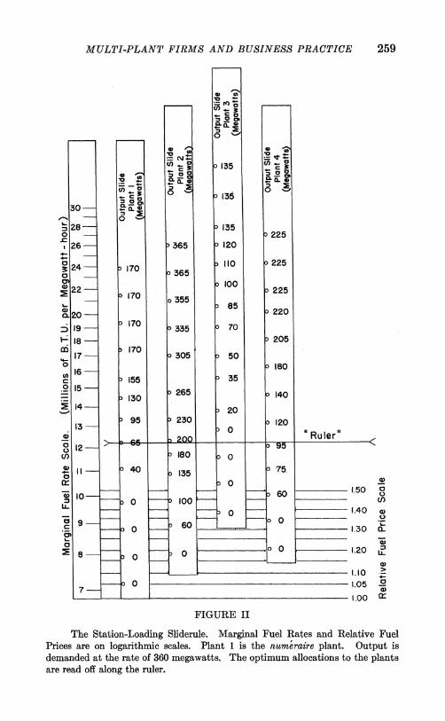
In order to facilitate the actual job of allocating the demanded electricity or "load" among plants in conformance with our theoreti- cal principles, a Station-Loading Sliderule was developed.8 This mechanical device permits a centrally located dispatcher, in constant communication with the plants, to calculate quickly the optimum allocations for each demand situation.
The essentials of the sliderule, shown schematically in Figure II, are two unmovable scales, the "marginal fuel rate scale" and the "relative fuel price scale," and as many movable "plant output slides" as there are plants in the system - one for each plant. Mar- ginal -fuel rates are the additional amounts of fuel required (in millions of B.T.U.) in a plant to produce extra units of output (in megawatt-
6. In this paper we shall ignore the complications that may arise if some of the system's electricity is generated in hydroelectric plants.
7. M. J. Steinberg and T. H. Smith, Economy Loading of Power Plants and Electric Systems (New York, 1943), pp. 141 ff.
8. Ibid., pp. 189 ff.
MULTI-PLANT FIRMS AND BUSINESS PRACTICE 259
0
I- ,. a. w 4 Cn 0 = 2~ 0
C 135
30 - a. -ll 0 S 28- 135 o 225 r-c i26- 365 0120
o ~~~~ ~~~~~110 225 3 24- 170 36
CP2 170100 25 10 o 355
a20 85 ~~~~~~~0220 10-820
170
C6 15503
4- 1730 265 140
0 ~ ~ 9 20120
0l >5 - 265 0__ __
(I) 180 013 14
14 0 7 0~ ~~~~~~~2 0~~~~~~~
*(i 10 (1
- D 40 135 0 75.~~~~~1.0 W9 0
U ~~~~~~~~~~~~~~~~1.30 Q
0 0~~~ 10U 1.20
7j; 0~~~~~~~~~~~~~
1.10 *
0 1.05 . 70
1.00 W-
FIGURE II
The Station-Loading Sliderule. Marginal Fuel Rates and Relative Fuel Prices are on logarithmic scales. Plant 1 is the nume'raire plant. Output is demanded at the rate of 360 megawatts. The optimum allocations to the plants are read off along the ruler.

260 QUARTERLY JOURNAL OF ECONOMICS
hours). They are reciprocals of marginal productivities. Relative fuel prices are the prices of fuel at each plant relative to the price of fuel at the plant with the lowest fuel price. We may call the latter plant(s) the numeraire plant(s).
The marginal fuel rate scale is calibrated with the logarithms of marginal fuel rates (log dv/dx), starting at the bottom with values somewhat below those actually to be encountered and increasing con- tinuously to some point at the top slightly greater than the largest value to be encountered in the system. Relative fuel prices are also on a logarithmic scale. This scale begins with log 1 - the index and runs alongside the marginal fuel rate scale. Each output slide is calibrated in such a way that when the bottom of the slide is lined up with the index on the fuel price scale, its markings show the maximum output rates in the plant that the slide represents corresponding to every marginal fuel rate.
In using the sliderule the dispatcher displaces each of the plant output slides (except that of the num6raire plant) from the index to the appropriate point on the relative fuel price scale. Thus, if the price of fuel at the numeraire plant is 25s? per million B.T.U. and at plant 2 the price is 30/, the bottom of the output slide of plant 2 is moved to 1.2 on the relative fuel price scale. To divide the output among plants so as to "equalize" marginal cost, he merely has to move a "ruler," crossing the output slides horizontally, to that posi- tion where the sums of the outputs marked on the slides along the ruler add up to the total demand - whatever it may be at the moment. These outputs of the individual plants satisfy the first order conditions for a minimum which we discussed above.9
Instead of equating marginal costs of the plants in operation, the dispatcher using this device actually equates
I W11 W2 (5a) log I + log - = log + log .... dx1/dV1 w1 dx2/dv2 w
But this is identically
(5b) logC1 = log 2 =. W1 W1
9. This sliderule is reminiscent of the one introduced by Edgeworth (Papers Relating to Political Economy, II, 52-58) to illustrate Mangoldt's contribution to the comparative cost doctrine in international trade theory. Cf. J. Viner, Studies in the Theory of International Trade, pp. 458-67.

MULTI-PLANT FIRMS AND BUSINESS PRACTICE 261
A moment's reflection will convince the reader that these equations have the same solutions as set (3).1 Also, as inspection of Figure II will show, the required inequalities will hold for all idle plants. Using logarithms of marginal costs is convenient when there is only one variable factor (input) because the marginal cost function is simply shifted without change in shape in response to price changes of the factor.
Fortunately, the complexities introduced by decreasing marginal costs can be ignored. The very nature of plant equipment insures that marginal fuel rates and hence marginal costs are increasing func- tions of output. Proper use of the sliderule will satisfy the first order necessary conditions and rising marginal cost curves at every plant make these conditions also sufficient for minimum cost allocation of output.
It should be noted that no essential complications arise, either in the theoretical solution or in its application, if marginal cost curves of the plants are discontinuous.2 In fact, in many systems some plants (the most modern and favorably located fuel-pricewise) are always used up to capacity.
IV The foregoing solution to the allocation problem is optimal only
if no variable costs or losses of electricity result from transporting the generated electricity from plants to consumers. Typically there are no variable transport costs as such once the system is built; but elec- trical energy is lost during the process of transmission. Such losses for a system, it was shown as recently as twelve years ago,3 can be expressed in terms of a quadratic form
n n
y =Y (XlYX2y . . . Y Xn) =; z Bijxixj , i=1 j=1
where y represents the loss in megawatts and the x's, as previously, are the outputs of the plants. Subsequently, methods were developed
1. Just as the equilibrium conditions in consumer theory are independent of monotonic stretchings of the "utility index," so the equilibrium conditions for a multi-plant firm are independent of such a "cost index."
2. Since, corresponding to each marginal fuel rate, the maximum output is marked on the plant's output slide, a discontinuity means that scheduled output for the plant in the neighborhood of the discontinuity will remain unchanged for several different values of the marginal fuel rate. Also, cf. Samuelson, op. cit., pp. 70 ff.
3. E. E. George, "Intrasystem Transmission Losses," Electrical Engineering (AIEE Transactions), Vol. 62 (March 1943), pp. 153-58.
262 QUARTERLY JOURNAL OF ECONOMICS
for deriving the loss formula coefficients, Bij, by means of network analyzers - miniature representations (electrical analogues) of the entire integrated generating and transmission system.4
A number of simplifying assumptions are made in the develop- ment of the formula and in the estimation of the coefficients. The most significant of these, from the economist's point of view, is that during the normal course of demand variations, the demands for elec- tricity at every point in the system are assumed to vary proportion- ately. This means that we may think of all the electricity actually sold to many consumers all along the system as if it were delivered to a single consumer located at a fixed delivery point. Should this assumption be unrealistic for a particular system, additional variables may be introduced into the formula, or a different set of coefficients may have to be used for each pattern of demand variations. But these complications will not concern us in this paper.'
The essence of the theoretical solution which makes allowances for transmission losses was worked out quite recently by electrical engineers. Again the problem is to minimize the firm's total costs, represented by equation (1), for each level of demanded output. But the simple "conservation-of-product constraint" (equation (2)) is no longer appropriate. There are losses which depend upon how much electricity each plant is producing. The new constraint becomes
n
(2') z xi = D + y(x1,x2 ... Xn). i=1
It simply says that the total electricity generated by all the plants together must add up to the total quantity demanded by consumers plus the quantity lost in transmission.
Proceeding as before, we can readily discover the necessary and sufficient conditions for minimum cost allocation.7 The first order
4. J. B. Ward, J. R. Eaton, H. W. Hale, "Total and Incremental Losses in Power Transmission Networks," AIEE Transactions, Vol. 69 (Part I, 1950), pp. 626-31.
5. Ibid., p. 629. 6. E. E. George, H. W. Page, and J. B. Ward, "Coordination of Fuel Cost
and Transmission Loss by Use of the Network Analyzer to Determine Plant Loading Schedules," AIEE Transactions, Vol. 68 (Part II, 1949), pp. 1152-60. L. K. Kirchmayer and G. W. Stagg, "Evaluation of Methods of Co-ordinating Incremental Fuel Costs and Incremental Transmission Losses," AIEE Trans- actions, Vol. 71 (Part III), 1952, pp. 513-20.
7. The Lagrangean expression to be minimized under constraint is C - ,(2;x - y - D).
MULTI-PLANT FIRMS AND BUSINESS PRACTICE 263
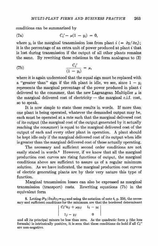
conditions can be summarized by
(7a) Ci'- i(1 - yj) = 0,
where ys is the marginal transmission loss from plant i (= 9y/axf); it is the percentage of an extra unit of power produced at plant i that is lost during transmission if the output of all other plants remains the same. By rewriting these relations in the form analogous to (3)
ci, (7b) (- = T where it is again understood that the equal sign must be replaced with a "greater than" sign if the ith plant is idle, we see, since 1 - represents the marginal percentage of the power produced in plant i delivered to the consumer, that the new Lagrangean Multiplier , is the marginal delivered cost of electricity - the marginal c.i.f. cost, so to speak.
It is now simple to state these results in words. If more than one plant is being operated, whatever the demanded output may be, each must be operated at a rate such that the marginal delivered cost of its output (the marginal cost of the output generated by it actually reaching the consumer) is equal to the marginal delivered cost of the output of each and every other plant in operation. A plant should be kept idle only if the marginal delivered cost of its output when idle is greater than the marginal delivered cost of those actually operating.
The necessary and sufficient second order conditions are not easily stated in words.8 However, if we know that all the marginal production cost curves are rising functions of output, the marginal conditions above are sufficient to assure us of a regular minimum solution. As we have indicated, the marginal production cost curves of electric generating plants are by their very nature this type of function.
Marginal transmission losses can also be expressed as marginal transmission (transport) costs. Rewriting equations (7b) in the equivalent form
8. Letting d9y/oxj(xj = yij and using the notation of note 4, p. 256, the neces- sary and sufficient conditions for the minimum are that the bordered determinant
Ci"Sij + Ayij 1i - Yi
lj - yj 0 and all its principal minors be less than zero. As the quadratic form y (the loss formula) is intrinsically positive, it is seen that these conditions do hold if all Ci" are non-negative.

264 QUARTERLY JOURNAL OF ECONOMICS
(7c) Ci, + gys = q, the marginal delivered cost, q, is seen to be the sum of the marginal production cost, Cj', and the marginal transmission loss, gyj -the marginal transmission loss "priced" at the marginal delivered cost.
Before proceeding with the explanation of how these results are brought to bear in actual practice in scheduling production of the generating plants, it may be helpful to show our theoretical solution graphically for a two-plant firm. For this purpose a diagram different from that used to illustrate the no-transmission-loss-case is conven- ient. In Figure III the electricity produced by plant 1 is plotted on the horizontal axis, that produced by plant 2 on the vertical. The family of curves labeled CaCbCC etc., are what I call Constant Outlay Curves. For a given rate of total expenditure by the firm, say Cb, the curve labeled Cb shows the maximum rate of output that
o K
0 K
Output of Plant I Xi FIGURE III
The points K, L, M, represent least-cost allocations of demanded output rates De, Df, Da, respectively. No allocations can be found for these demand situations which lie on lower Constant Outlay Curves. can be produced in plant 2 for each specified output rate of plant 1. The further such curves are away from the origin, the greater is the outlay (total expenditure) identified with them. Their slopes are - C1'/C2'- the ratio of marginal production costs in plant 1 to those in plant 2; and if we know that marginal production costs. in the plants are increasing functions of output, we can be sure that the Constant Outlay Curves are concave to the origin. The other set of curves, D eDf D&, etc., are what we may call Allocation Possibility Curves. If consumers demand electricity at the rate, say De, the
MULTI-PLANT FIRMS AND BUSINESS PRACTICE 265
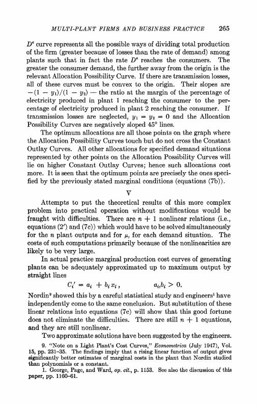
De curve represents all the possible ways of dividing total production of the firm (greater because of losses than the rate of demand) among plants such that in fact the rate De reaches the consumers. The greater the consumer demand, the further away from the origin is the relevant Allocation Possibility Curve. If there are transmission losses, all of these curves must be convex to the origin. Their slopes are - (1 - y1)/(l - Y2) - the ratio at the margin of the percentage of electricity produced in plant 1 reaching the consumer to the per- centage of electricity produced in plant 2 reaching the consumer. If transmission losses are neglected, Yi = Y2 = 0 and the Allocation Possibility Curves are negatively sloped 450 lines.
The optimum allocations are all those points on the graph where the Allocation Possibility Curves touch but do not cross the Constant Outlay Curves. All other allocations for specified demand situations represented by other points on the Allocation Possibility Curves will lie on higher Constant Outlay Curves; hence such allocations cost more. It is seen that the optimum points are precisely the ones speci- fied by the previously stated marginal conditions (equations (7b)).
V Attempts to put the theoretical results of this more complex
problem into practical operation without modifications would be fraught with difficulties. There are n + 1 nonlinear relations (i.e., equations (2') and (7c)) which would have to be solved simultaneously for the n plant outputs and for ,u, for each demand situation. The costs of such computations primarily because of the nonlinearities are likely to be very large.
In actual practice marginal production cost curves of generating plants can be adequately approximated up to maximum output by straight lines
Ci' as + bi xi ai,bi > O.
Nordin9 showed this by a careful statistical study and engineers' have independently come to the same conclusion. But substitution of these linear relations into equations (7c) will show that this good fortune does not eliminate the difficulties. There are still n + 1 equations, and they are still nonlinear.
Two approximate solutions have been suggested by the engineers. 9. "Note on a Light Plant's Cost Curves," Econometrica (July 1947), Vol.
15, pp. 231-35. The findings imply that a rising linear function of output gives significantly better estimates of marginal costs in the plant that Nordin studied than polynomials or a constant.
1. George, Page, and Ward, op. cit., p. 1153. See also the discussion of this paper, pp. 1160-61.

266 QUARTERLY JOURNAL OF ECONOMICS
Both have been verified by actual sample calculations to yield alloca- tions extremely close to the theoretical optimum. The first, a linear approximation,2 is obtained by replacing on the left of each equation (7c) the variable ,u with a constant y: (8a) CZ + Yyi = i
Making use of the linear estimates of the marginal cost curves and substituting for yi the partial derivatives of the loss formula this becomes
n
(8b) ai + bitx + y(2 2 Bijxj) = In j=1
The new constantly is a weighted average value of marginal delivered costs , and is used to "price" the transmission losses. Note that these are linear relations in the unknowns. Even if inequalities replace some equalities for certain values of demanded output, the allocations corresponding to each u, hence by equation (2') for each level of delivered output, may be obtained without difficulties by the use of modern high-speed electronic computing equipment.
The other approximation, now actually used in the American Gas and Electric Company System, is called the "Penalty Factor Method."3 Rather than "pricing" transmission losses at actual mar- ginal delivered costs (g), as in the exact solution, or at some average value of marginal delivered costs (-y), as in the linear approximation, this method charges for them at the marginal production costs of each plant in question (Ci'). The equations (7c) then become (9a) CZ + Ci'yi = CZ'(l + yi) = 4; or substituting for yi,
n
(9b) Cil(1 + 2 2 Bijxj) = j, j=1
The term 1 + yj is called the "penalty factor" for plant j.4 These penalty factors can be efficiently calculated for each plant under numerous operating conditions of the system.5
An advantage of this method is that it permits continued use of the Station-Loading Sliderule, which, as will be recalled, does not require linear approximations or, for that matter, continuity of the
2. Loc. cit. 3. L. K. Kirchmayer and G. H. McDaniel, "Transmission Losses and
Economic Loading of Power Systems," General Electric Review, Vol. 54 (Oct. 1951), pp. 39-46. Also, Kirchmayer and Stagg, op. cit.
4. The "penalty factor" consists of the first two terms of the expansion of 1/1 - y in the exact formulation, equations (7b).
5. The Wall Street Journal, August 12, 1953, p. 18, reported the purchase of a $110,000 electronic computer by the American Gas and Electric Company for calculating "penalty factors."
MULTI-PLANT FIRMS AND BUSINESS PRACTICE 267
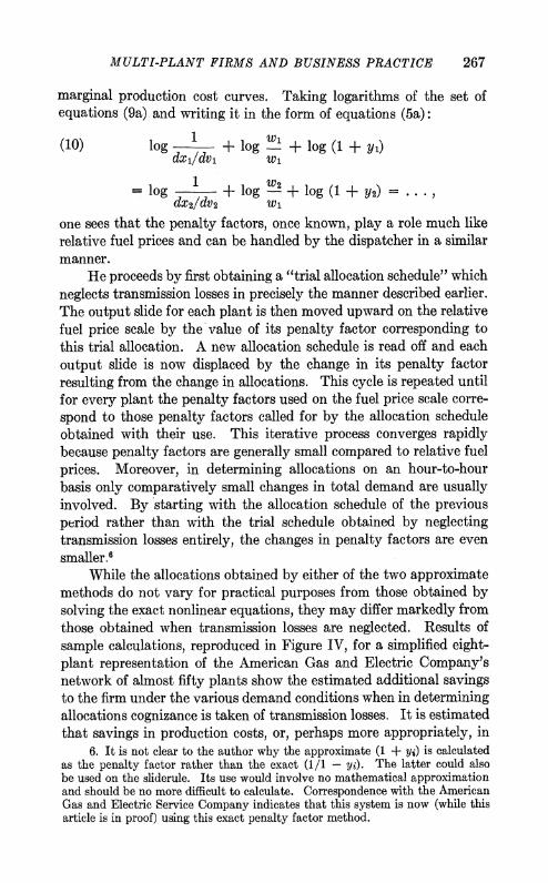
marginal production cost curves. Taking logarithms of the set of equations (9a) and writing it in the form of equations (5a):
(10) log + log Wi + log (1 + y) dxl/dv1 Wi
-log + log W2 + 109 (I + Y2) dx2/dv2 Wi
one sees that the penalty factors, once known, play a role much like relative fuel prices and can be handled by the dispatcher in a similar manner.
He proceeds by first obtaining a "trial allocation schedule" which neglects transmission losses in precisely the manner described earlier. The output slide for each plant is then moved upward on the relative fuel price scale by the value of its penalty factor corresponding to this trial allocation. A new allocation schedule is read off and each output slide is now displaced by the change in its penalty factor resulting from the change in allocations. This cycle is repeated until for every plant the penalty factors used on the fuel price scale corre- spond to those penalty factors called for by the allocation schedule obtained with their use. This iterative process converges rapidly because penalty factors are generally small compared to relative fuel prices. Moreover, in determining allocations on an hour-to-hour basis only comparatively small changes in total demand are usually involved. By starting with the allocation schedule of the previous period rather than with the trial schedule obtained by neglecting transmission losses entirely, the changes in penalty factors are even smaller.'
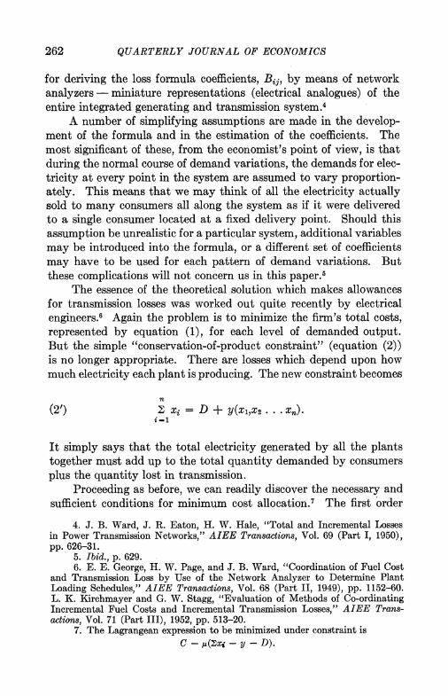
While the allocations obtained by either of the two approximate methods do not vary for practical purposes from those obtained by solving the exact nonlinear equations, they may differ markedly from those obtained when transmission losses are neglected. Results of sample calculations, reproduced in Figure IV, for a simplified eight- plant representation of the American Gas and Electric Company's network of almost fifty plants show the estimated additional savings to the firm under the various demand conditions when in determining allocations cognizance is taken of transmission losses. It is estimated that savings in production costs, or, perhaps more appropriately, in
6. It is not clear to the author why the approximate (1 + yi) is calculated as the penalty factor rather than the exact (1/1 - ye). The latter could also be used on the sliderule. Its use would involve no mathematical approximation and should be no more difficult to calculate. Correspondence with the American Gas and Electric Service Company indicates that this system is now (while this article is in proof) using this exact penalty factor method.
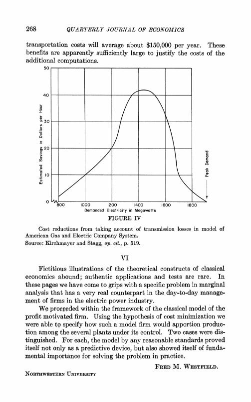
268 QUARTERLY JOURNAL OF ECONOMICS
transportation costs will average about $150,000 per year. These benefits are apparently sufficiently large to justify the costs of the additional computations.
50 -
40 - 10 0 6 8
I~~~~~V
0
C12 0 -
Fctiiu ilutain ftetertclcntutfclsia
20~~~~~~~~~~~~~~ C 0~~~~~~~~~~~~~~~~~~~~~~~~~~~~~~~~~~~)
E 1i0 at h v a n t e
0 V 80 1000 1200 1400 1600 1800
Demanded Electricity in Megawatts
FIGURE IV
Cost reductions from taking account of transmission losses in model of American Gas and Electric Company System. Source: Kirchmayer and Stagg, op. cit., p. 519.
VI
Fictitious illustrations of the theoretical constructs of classical economics abound; authentic applications and tests are rare. In these pages we have come to grips with a specific problem in marginal analysis that has a very real counterpart in the day-to-day manage- ment of firms in the electric power industry.
We proceeded within the framework of the classical model of the profit motivated firm. Using the hypothesis of cost minimization we were able to specify how such a model firm would apportion produc- tion among the several plants under its control. Two cases were dis- tinguished. For each, the model by any reasonable standards proved itself not only as a predictive device, but also showed itself of funda- mental importance for solving the problem in practice.
FRED M. WESTFIELD. NORTHWESTERN UNIVERSITY