Marginal Abatement Cost Curves: Combining Energy System

Modelling and Decomposition Analysis*

Fabian Kesickia

a Energy Institute

University College London

14 Upper Woburn Place

London WC1H 0HY, United Kingdom

E-mail: fabian.kesicki.09@ucl.ac.uk

Abstract

Various policies have been implemented in the last decade to tackle rising greenhouse gas

emissions. In this context it remains an open question of how to find a cost-efficient approach

to climate change mitigation. Marginal abatement cost (MAC) curves are a useful tool to

communicate findings on the technological structure and the economics of CO2 reduction to

decision makers. Existing ways of generating MAC curves fail to combine technological

detail in the graphical representation with the incorporation of system-wide interactions and a

framework for uncertainty analysis. This paper suggests a new approach to overcome the

present shortcomings by using a bottom-up energy system model in combination with index

decomposition analysis. For illustration purposes, this technique is applied to the transport

sector of the United Kingdom in scenarios with varied fossil fuel production cost assumptions

for the year 2030. The resulting MAC curves are found to be relatively robust to different fuel

costs. The findings indicate that CO2 reduction comes first from fuel decarbonisation, i.e.

electricity, hydrogen and diesel, and at higher CO2 prices from structural shifts. A minor

contribution to emission savings comes from demand reduction, while efficiency

improvements do not contribute to emission savings.

*The support of a German Academic Exchange Service (DAAD) scholarship is gratefully acknowledged.

UCL ENERGY INSTITUTE

- 2 -

1 Introduction

Legal commitments in the form of the Kyoto Protocol, the European Union 20-20-20 goals or

the United Kingdom (UK) Climate Change Act confront policy makers in many countries

around the world with the challenge of reducing carbon emissions in a cost-efficient way. For

this purpose, marginal abatement cost (MAC) curves have frequently been used to illustrate

the economics of climate change mitigation and have contributed to decision making in the

context of climate policy. In the UK, MAC curves have recently played an important role in

shaping the government’s climate change policy. Policy makers have relied on two types of

abatement cost curves: expert-based (Committee on Climate Change 2008) and model-

derived curves (Carmel 2008). The UK government used those abatement curves as a guide to

the potential and future costs of technical measures for its UK Low Carbon Transition Plan

(HM Government 2009).

The concept of abatement curves has been applied since the early 1990s to illustrate the costs

associated with carbon abatement and to serve as a decision making aid for environmental

policy. A MAC curve is defined as a graph that indicates the marginal cost of emission

abatement for varying amounts of emission reduction. In a policy context, the use of these

curves is not only restricted to incentive-based policies based on a CO2 tax or carbon emission

trading, but it can also give valuable insights concerning “command-and-control” regulations,

e.g. technical norms or standards, to overcome market imperfections in the field of energy

efficiency and conservation in buildings, industry and transport. Furthermore, it can indicate

necessary information for research and development spending, e.g. the implementation of

subsidies for emerging technologies.

However, there are some weaknesses associated with the concept of MAC curves. Abatement

costs are shown only for a specific point in time, generally for one particular year.

Nevertheless, the shape of the MAC curve depends on the cumulative emission reduction, that

means actions in earlier and later time periods have an influence. Thus, the MAC curve is

subject to intertemporal dynamics. Moreover, MAC curves usually include direct costs, i.e.

the cost reduction of ancillary benefits is not considered in the abatement cost. Finally, MAC

curves generally do not give any indication of the uncertainties involved in carbon dioxide

emission reduction.

- 3 -

MAC curves take on many forms: they may differ in regard to the regional scope, the time

horizon, the sectors included and the approach used for their generation. According to the

underlying methodology, MAC curves can be divided into expert-based and model-based

abatement cost curves (Fig. 1). For a detailed discussion of both approaches see Kesicki

(2010).

Expert-based approaches are built upon assumptions for the emission reduction potential and

the corresponding cost of single measures (including new technologies and efficiency

improvements). Subsequently, the measures are ranked from cheapest to most expensive to

represent the costs of achieving incremental levels of emissions reduction (see e.g. Jackson

1991; Naucler et al. 2009). The principal advantage of expert-based abatement cost curves is

that they are easy for policy makers to understand and that the marginal costs and the

abatement potential can be unambiguously assigned to one mitigation option. The key

disadvantages are that this approach does not take into account interdependencies within the

energy system, behavioural aspects, nor intertemporal interactions and is susceptible to

inconsistent baseline assumptions.

Fig. 1: Example for an expert-based (left) and model-derived MAC curve (right)

Another widespread approach is to derive the cost and potential for emission mitigation from

energy model runs. A common way is to distinguish models into economy-orientated top-

down models and engineering-orientated bottom-up models (Hourcade et al. 1995). In both

cases, abatement curves are generated by summarising in a curve the CO2 price resulting from

runs with different strict emission limits or the emissions resulting from different CO2 prices

(see e.g. Viguier et al. 2003). The cost definition considered in model-based approaches is

wider than in expert-based curves, i.e. it includes sectoral costs for bottom-up models and

macroeconomic costs for top-down models. Drawbacks of MAC curves generated by top-

0

50

100

150

0 10 20 30 40 50

Mar

gin

al A

bat

em

en

t C

ost

[$

/t C

O2]

Emission Abatement [Mt CO2]

- 4 -

down models include the lack of technological detail in the graphical representation, disregard

of market distortions and the reliance on historic data for the calculation of future abatement

costs. MAC curves generated by bottom-up models include only direct costs in the energy

system, do not present any technological detail in the abatement curve and marginal

abatement costs can be diluted by other constraints.

It should also be noted that cost and abatement potential definitions vary between different

approaches. While expert-based curves consider technology costs, bottom-up models use

sectoral costs, which include in addition to technology and fuel related costs also indirect

costs within the whole sector, such as costs of foregone demand. Top-down models

incorporate as well indirect costs impacts on other sectors. Concerning the abatement

potential, model-derived curves rely on the market potential. In contrast to the technical

abatement potential, used by expert-based curves, it considers market conditions including

market barriers, technological, behavioural and intersectoral interactions and policies in place

(see also Halsnaes et al. 2007).

So far, no MAC curve has been constructed that presents the technological detail based on

consistent assumptions, while being able to take into account technological, intertemporal,

economic and behavioural interactions and to provide a framework for a structured

consideration of uncertainty. The goal of this paper is to present a new approach to generate

MAC curves by combining energy system modelling, decomposition analysis and uncertainty

analysis in order to overcome the shortcomings of existing approaches.

The next section presents the general approach to generate MAC curves via the use of an

energy system model and decomposition analysis. Section 3 gives an application of the new

approach for the transport sector, where two scenarios with different assumptions on fossil

fuel production costs are analysed. Finally, the paper is concluded with section 4, which

argues that reductions in the carbon intensity of energy carriers and structural changes are the

important sources of emission reduction in the UK transport sector.

2 Methodology

In order to overcome the shortcomings in present approaches, the approach outlined in this

paper combines energy system modelling with decomposition and uncertainty analysis. An

energy system model is used to derive MAC curves via model runs with different price paths.

In the next step, the change in model results is decomposed to attribute the emission reduction

- 5 -

to demand reduction, efficiency improvements, structural changes and changes in the carbon

intensity of secondary energy carriers. Finally, uncertainty analysis, in this paper in the form

of sensitivity analysis, highlights the robustness of the abatement cost in respect to changes in

key assumptions and drivers, e.g. fuel prices.

The benefits of this approach are that it incorporates all the advantages of a model-based

approach, while bringing in the technological detail into MAC curves usually attained through

expert judgments. However, this approach does not address the existing problem of taking

into account the effect of ancillary benefits on the abatement costs. Thus, the calculation

considers only the direct cost of CO2 abatement and presents an upper limit of actual

abatement costs. In addition, the model is not able to capture all micro- and macro-economic

interactions, e.g. market distortions or economy wide feedbacks.

2.1 Energy System Modelling

For the calculation of MAC curves an energy-economic model-based approach provides a

solid theoretical basis, through a technologically explicit, partial equilibrium, consistent

optimisation framework. This approach encapsulates sectoral detail, energy supply chain

infrastructures, direct as well as indirect effects on markets and prices, and an explicit

treatment of mitigation options. Hence, such a systems approach serves as a base to calculate

abatement cost curves taking into account interactions between mitigation measures. The

MARKAL (MARKet ALlocation) energy model, developed within the International Energy

Agency’s ETSAP consortium, is used within this context.

MARKAL is a dynamic, technology-rich linear programming (LP) energy systems

optimisation model. In its elastic demand formulation, accounting for the response of energy

service demands to prices, its objective function maximises producer and consumer surplus

under conditions of perfect foresight. MARKAL portrays the entire energy system from

imports and domestic production of energy carriers through to fuel processing and supply,

explicit representation of infrastructures, conversion of fuels to secondary energy carriers,

end-use technologies and energy service demands of the entire economy. A wide-ranging

application of policy and physical constraints, implementation of taxes and subsidies, and

inclusion of base-year capital stocks and energy flows, enable the calibration of a model to a

particular energy system. Full details of the optimisation methodology is given in Loulou et

al. (2004).

- 6 -

In the MARKAL model for the UK (Anandarajah et al. 2008) resource supply curves

represent a key input parameter for the model. From these baseline costs, multipliers are used

to generate both higher cost supply steps as well as imported refined fuel costs. A second key

input is dynamically evolving technology costs. Future costs are based on expert assessment

of technology vintages or, for less mature electricity and hydrogen technologies, via

exogenous learning curves derived from an assessment of learning rates combined with global

forecasts of technology uptake. A third key input is an explicit depiction of infrastructures,

physical and policy constraints. A final key input for the UK MARKAL model are exogenous

demands for energy services, which are derived from standard UK forecasts for residential

buildings, transport, service and industry sectors. Generally, these sources entail a low energy

growth projection with saturation effects in key sectors. This is reflective of recent historical

trends on sustained modest economic growth and the continuing dematerialisation of the UK

economy.

In the transport sector of the UK MARKAL model, the energy service demands, measured in

billion vehicle kilometres, are included for various modes of transport: Air Travel, Car

Travel, Bus Travel, Heavy Goods Vehicles (HGV), Light Goods Vehicle (LGV), Rail

Transport and Two-wheeler. In addition, it has a number of fuel distribution networks to track

fuel use by mode of transport. To meet the different transport energy service demands, a

number of vehicle technologies are integrated in the model. Those include amongst others

petrol cars, hydrogen cars, ethanol LGVs, hybrid and electric cars. A number of key data

parameters that are required to characterise the transport vehicle technologies, such as

technical efficiency of a vehicle, capital cost, vehicle lifetime or annual kilometres usages, are

defined in the model.

A comprehensive description of the UK model, its applications and core insights can be found

in Strachan et al. (2008), and in the model documentation (Kannan et al. 2007).

2.2 Decomposition Analysis

Decomposition analysis (in this paper used as a synonym for index decomposition analysis)

helps to bring technological detail in the representation of the MAC curve. This technique is a

well established research methodology to decompose an aggregated indicator, usually either

energy use or CO2 emission, into its drivers (see Ang et al. 2000). After the two oil price

shocks in the 1970s, this technique has been used to determine the factors behind historical

industrial energy use and to analyse ways to reduce future energy consumption in the industry

- 7 -

sector (Hankinson et al. 1983). In the 1990s the focus of decomposition shifted from energy

use towards CO2 emission (see e.g. Torvanger 1991) based on the Kaya identity (Kaya 1989).

Over the course of the 1990s and the early 21st century there have been numerous studies for

different regions and energy sectors that have tried to find the underlying causes of CO2

emission development with the help of various decomposition techniques (see e.g. Diakoulaki

et al. 2006; Shrestha et al. 2009).

Decomposition of CO2 emissions can be described as a series expansion truncated at first

order, so that a residual of higher order remains. To avoid this problem, several methods have

been developed in the last few years to distribute the residual among the factors. So far,

decomposition analysis has always been applied through time to gain insights into the

development of emissions in recent or future decades. This has not been extended to a

decomposition along rising CO2 taxes to obtain a technologically detailed MAC curve.

In this study, the resulting CO2 emission in the transport sector are decomposed into four

different effects: activity effect, structure effect, fuel intensity effect and carbon intensity

effect:

(1)

The activity is the energy service demand in billion vehicle kilometres, fueli,j describes the

amount of fuel that is necessary to satisfy demand i with technology j. CO2,Transport,i,j represent

the amount of CO2 released by the use of technology j to satisfy demand i. Equation (1) can

be rewritten into:

(2)

In this equation the four factors correspond to the factors in equation (1), where a is the

activity variable, s stands for structure, f for fuel intensity and c for carbon intensity.

The emphasis is not on an absolute number but on what influences the change in CO2

emissions in the transport sector:

- 8 -

(3)

In the past there have been many approaches to distribute the residual terms to the other

variables in order to achieve a so-called perfect decomposition (Ang 2004). This is regarded

as easier to interpret as it does not include a residual term. In this study the Logarithmic Mean

Divisia Index (LMDI) is used. This index is based on the Divisia index (Divisia 1925) and the

logarithmic mean (Montgomery 1937; Vartia 1976) and was applied the first time in the

context of energy and emissions by Ang et al. (1998). The LMDI is used because it leaves no

residual and therefore gives a perfect decomposition. Furthermore, it does not differ

significantly from other perfect decomposition methods and its calculation is comparably

easy. Detailed calculation of the LMDI and its application to the different effects can be

found in the Appendix.

2.3 Uncertainty Analysis

Marginal abatement costs and abatement potentials are subject to important uncertainties.

Thus, results depend on key drivers and assumptions such as discount rate, fuel prices,

technology costs and demand development. The consideration of uncertainty in the form of

sensitivity analysis, stochastic analysis or probabilistic assessment can help to draw

conclusions about the robustness of a MAC curve.

In this paper, two scenarios with different assumptions on the production costs of fossil fuels

are presented. The high fossil fuel production cost scenario assumes domestic production

costs and import costs for fossil fuels (natural gas, oil, hard coal, coking coal) to be twice as

expensive as in the low cost scenario.

3 Results

The transport sector was chosen for this analysis because over the past three decades CO2

emissions grew the fastest in the transport sector in the UK, from 71 Mt CO2 in 1970 to

around 135 Mt CO2 in 2007. The transport sector is now responsible for a quarter of all CO2

emissions compared to ten percent in 1970 (AEA Energy & Environment 2008). In the light

of a predicted rising demand for transport services, the transport sector will be a pivotal

element in any strategy to reduce CO2 emissions.

- 9 -

To generate a MAC curve, scenarios with different model-wide CO2 prices are generated. The

CO2 price increases over time from 2000 to 2050 with the discount rate inherent to the model

of 5% p.a. The CO2 price is varied between £2000 0 per ton CO2 to £2000 219 per ton CO2 for

the year 2030 (long-term exchange rate £=1.4€), corresponding to £2000 580 per ton CO2 in

2050. A CO2 price of £100/t CO2 corresponds to an increase of about £47 for a barrel of crude

oil. In this way, 46 scenarios with different CO2 prices are calculated and later on

consolidated to a MAC curve. Two MAC curves were generated for 2030 with different

assumptions concerning the production costs of fossil fuels. All prices are given in £2000.

3.1 System-wide MAC Curve

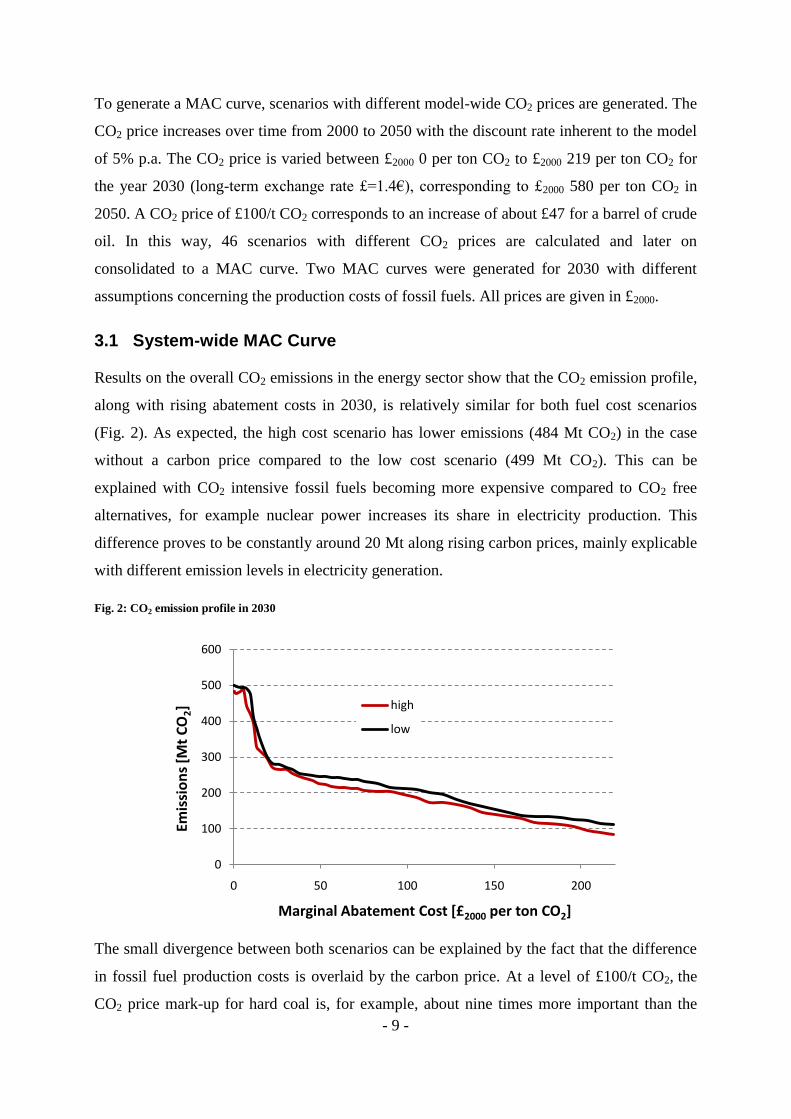
Results on the overall CO2 emissions in the energy sector show that the CO2 emission profile,

along with rising abatement costs in 2030, is relatively similar for both fuel cost scenarios

(Fig. 2). As expected, the high cost scenario has lower emissions (484 Mt CO2) in the case

without a carbon price compared to the low cost scenario (499 Mt CO2). This can be

explained with CO2 intensive fossil fuels becoming more expensive compared to CO2 free

alternatives, for example nuclear power increases its share in electricity production. This

difference proves to be constantly around 20 Mt along rising carbon prices, mainly explicable

with different emission levels in electricity generation.

The small divergence between both scenarios can be explained by the fact that the difference

in fossil fuel production costs is overlaid by the carbon price. At a level of £100/t CO2, the

CO2 price mark-up for hard coal is, for example, about nine times more important than the

Fig. 2: CO2 emission profile in 2030

0

100

200

300

400

500

600

0 50 100 150 200

Emis

sio

ns

[Mt

CO

2]

Marginal Abatement Cost [£2000 per ton CO2]

high

low

- 10 -

difference in production costs. To a lesser extent this holds true for other fossil fuels. Fig. 3

gives an overview of fuel prices for hard coal, heavy fuel oil and natural gas for different CO2

prices. One can see that the relative difference between the fossil fuel prices in the industry

sector decreases with increasing carbon prices. While natural gas is 70% more expensive in

the high cost scenario compared with the low cost scenario in the case of no CO2 price, this is

reduced to 18% in the case of £200/t CO2. For hard coal the difference in the £200 case is

only 4%. In addition, the fuel prices converge as natural gas is the most expensive fuel in the

base case, but is less carbon intensive than coal and oil so that its price increases more slowly

with an increasing CO2 price.

The small difference concerning the fuel prices in the demand sectors, despite a 100%

increase in fossil fuel production cost, can be explained by several factors. The production

costs are only a small part of the price faced by different end-use sectors, such as industry or

transport. In addition to the production costs, the price includes distribution costs, refining

costs (in the case of crude oil) and domestic energy taxes. Furthermore, in the high cost

scenario fewer fossil fuels are consumed so that cheaper domestic reserves and cheaper

imports will be used to a limited extent along the supply cost curve.

Fig. 3: Industry fuel prices for different CO2 prices (dark bars: low fossil fuel production costs / light bars: high fossil

fuel production costs)

The emission profile in Fig. 2 showed a rapid decrease of emissions up to £20/t CO2 of 43%

followed by a rather gradual decrease up to £200/t CO2, where about 20% of the initial

emission level is attained.

0

2

4

6

8

10

12

14

16

18

20

£0 £100 £200 £0 £100 £200 £0 £100 £200

Hard Coal Heavy Fuel Oil Natural Gas

Pri

ce [

£2

00

0/G

J]

- 11 -

A MAC curve for the whole energy sector showing the contribution of each sector gives

insights into the abatement structure (Fig. 4). The height of each bar represents the marginal

abatement cost, while the width represents the emission abatement and the colour indicates

the sector.

Fig. 4: Marginal Abatement Cost Curve for the UK Energy Sector in 2030 (low fossil fuel production costs)

One can see that the rapid decrease in emissions up to £20/t CO2 originates in the supply

sector. The electricity sector and the hydrogen sector reduce emissions rapidly by shifting

from a carbon intensive production towards coal-fired power plants with carbon capture and

storage (CCS) and with further increasing carbon prices to electricity production from nuclear

power plants. The end-use sectors start to contribute to an emission reduction at about £40/t

CO2. While there are some comparably inexpensive mitigation options in the residential

sector, the industry sector proves to be harder to decarbonise. The transport sector achieves

most of the emissions reduction in a range of £100-£150/t CO2 through structural shifts in the

vehicle pool and, to a much more limited extent, through reductions in demand for energy

services.

3.2 Transport Sector

Including the results of the decomposition analysis shows which technologies are responsible

for the emission reduction. In this analysis of the transport sector, emissions occurring in

- 12 -

supply sectors for the production of secondary energy carriers used in the transport sector

have been assigned to this sector. Fig. 5 shows that structural shifts and the decarbonisation of

fuels are responsible for the majority of emission reduction in the low cost scenario. Demand

reduction due to higher costs for energy service demands represent a constant but minor

contribution. The demand contribution is limited due to structural changes that keep the price

for energy service demand relatively constant. In addition, one can distinguish three major

trends in the MAC curve.

Firstly, the cheapest option to reduce transport emissions is the decarbonisation of electricity,

since electricity is used as an energy input for almost all trains and a significant proportion of

cars in the £0/t CO2 case. Major structural changes away from coal fired power plants to coal

CCS plants and with higher carbon prices to nuclear plants are responsible for this

development. This plays a major role up to £35/t CO2, where electricity is decarbonised by

about 87% in 2030. Once electricity is sufficiently decarbonised, battery vehicles are used to

a greater extent. This starts at £13/t CO2 for buses and from around £140/t CO2 for cars.

Secondly, hydrogen is decarbonised between £15/t CO2 to £50/t CO2 by about 80%. This is

the consequence of hydrogen production shifting first towards natural gas and from around

£30/ t CO2 to hydrogen production from coal CCS plants. Furthermore, a switch to hydrogen

from electrolysis becomes more important with the ongoing decarbonisation of electricity.

The decarbonisation of hydrogen results in an important emissions reduction because a

significant portion of buses and heavy goods vehicles rely on hydrogen as a fuel in 2030 in

the case without any CO2 price. Furthermore, significant emissions mitigation is achieved

through a shift from diesel to hydrogen heavy good vehicles in the range of £50-£115/t CO2.

A third trend concerns cars and light goods vehicles consuming diesel. Diesel is decarbonised

between £80 and £160/t CO2, mainly due to the higher share of Fischer-Tropsch biodiesel

generated from solid biomass, but also due to limited import of biodiesel. The decarbonisation

of this secondary energy carrier via the increase of the share of biodiesel reduces the CO2

emissions from transport modes relying on diesel, i.e. bus, car, LGV and HGV. Above £150/t

CO2, one can observe a switch to diesel hybrid cars and to a minor extent to diesel plug-in

cars that rely on low carbon fuels and help to further reduce emissions.

- 13 -

Fig. 5: Marginal Abatement Cost Curve for the UK Transport Sector in 2030 (low fossil fuel production costs)

Each bar represents the marginal mitigation measure, i.e. the measure responsible for the emission reduction between two

adjacent CO2 price scenarios. Because of the dynamic model character the bars cannot be added together to form a total.

Fig. 6: Marginal Abatement Cost Curve for the UK Transport Sector in 2030 (high fossil fuel production costs)

Each bar represents the marginal mitigation measure, i.e. the measure responsible for the emission reduction between two

adjacent CO2 price scenarios. Because of the dynamic model character the bars cannot be added together to form a total.

- 14 -

In a further step, the assumptions on the fossil fuel production costs were doubled to make a

statement on the robustness of the abatement curve concerning the level of fuel prices. Fig. 6

shows the resulting MAC curve for the high fuel price scenario. The MAC curve looks very

similar in both cases as the emissions profile suggested. The emissions in the high cost

scenario are slightly less than in the low cost scenario due to the lower carbon intensity of

electricity. Differences can be observed in the decarbonisation of electricity, where nuclear

power plants play a much more important role. This can be explained with relative cost

advantages for uranium compared to increased hard coal production costs. At a price of £20

per ton CO2, the emissions reduction amount to 26 Mt CO2 in the low cost scenario and to 36

Mt CO2 in the high fuel scenario, which results from a higher decarbonisation of electricity

and hydrogen.

A major difference is that in the high fuel price scenario from £135/t CO2 on a higher share of

ethanol is used as a fuel for cars. This is seen in a higher share of E85 cars, which are able to

use a share of up to 85% ethanol in the fuel mix. In conclusion, additionally to the three

decarbonisation paths described above for the low cost scenario, ethanol plays a more

important but still limited role in the high cost scenario.

Concerning the decomposed MAC curve it has to be taken into account that this is a static

representation of a dynamic energy system. This means that the bars in Fig. 5 and Fig. 6

represent the marginal measure responsible for emissions mitigation. It may be possible,

however, that an earlier marginal abatement measure drops out of the carbon reduction

portfolio at higher carbon prices. The decomposed MAC curve indicates relatively large

emission reduction amounts due to electricity decarbonisation through a shift to coal CCS

power plants and at higher carbon prices a minor contribution form a further decreasing

carbon intensity of electricity generated from nuclear power. The contribution from nuclear

power plants is lower because electricity is already decarbonised to a large extent and only the

difference in carbon intensity between coal CCS and nuclear power plants is accounted for.

This phenomenon is further illustrated in the composition of electricity generation over rising

carbon prices (Fig. 7).

- 15 -

Fig. 7: Composition of electricity generation in 2030 (low fossil fuel production costs)

Electricity generation is dominated by coal in the base case and shifts to coal CCS at around

£20/t CO2, which significantly reduces CO2 emissions. Additional emissions reductions are

achieved more gradually from £50 to £150 per ton CO2 via the rising importance of nuclear

power for electricity generation. This is explained by the fact that nuclear power does not

emit CO2, while CCS plants are only able to reduce emissions from fossil fuels by around

90%. Thus, while coal CCS is the most cost-efficient option for CO2 mitigation from £20 to

£100/ t CO2, this is no longer the case for higher carbon prices.

In order to obtain an idea of the overall contribution of different effects for the emissions

reduction up to the highest CO2 price of £2000 219/t CO2, Fig. 8 summarises the results for the

activity, structure, efficiency and carbon intensity effects. The activity effect, i.e. a reduction

in the demand for energy services caused by higher prices, plays only a minor but constant

contribution. A reduction in fuel intensity or efficiency gains does not contribute to emissions

reduction in the transport sector. This means that carbon prices do not present an incentive for

efficiency gains in addition to those present in the base case. Reasons for this are that possible

efficiency gains are relative small in the order of a few percent and affect only a limited

portion of the entire vehicle fleet. More important, though, structural changes dominate the

transport sector and road vehicles have an average life time of 7 to 15 years, consequently

0

200

400

600

800

1000

1200

1400

1600

1800

2000

Ele

ctri

city

Ge

ne

rati

on

[PJ

]

Marginal Abatement Cost [£2000/t CO2]

Biomass & others CHPCoke CHPCoal CHPStorageImportWindTidalBiomass & othersHydroNuclearNatural GasCoal CCSCoal

- 16 -

investments into more efficient vehicles are not realised due to the anticipated switch to a

different technology.

The most important effects for carbon reduction are structural changes and the

decarbonisation of hydrogen, diesel and electricity. 37% of total carbon reduction is

originated from structural changes in the transport sector. This is shared between shifts to

hydrogen, diesel hybrid, battery and E85 vehicles. While structural changes towards battery

buses and cars play the most important role, E85 vehicles play a minor role. The carbon

intensity effect contributes 58% percent towards overall carbon reduction. This stresses the

importance of the supply sectors and the corresponding decarbonisation of secondary energy

carriers in order to achieve mitigation targets for the transport sector. In this context, the

contribution of decarbonisation of hydrogen, electricity and diesel via a higher share of

biodiesel is on a comparable level. In conclusion, the reduction of carbon intensive energy

carriers and structural changes are pivotal to a decarbonisation of the transport sector, where

structural changes are in general preceded by a decarbonisation of the concerned energy

carrier.

Fig. 8: Decomposition of CO2 reduction: £218 scenario compared to base case (low fossil fuel production costs)

4 Conclusions

In order to overcome a lack of technological detail in model-based approaches and the

disregard of system-wide interactions, a new approach is proposed combining a bottom-up

0

10

20

30

40

50

60

70

Activity Structure EfficiencyCarbon Intensity

Tota

l CO

2m

itig

atio

n [

Mt

CO

2] Hydrogen

Petrol/Ethanol

Diesel/Biodiesel

Electricity

Structure Diesel Plug-in

Structure E85

Structure Battery

Structure Diesel Hybrid

Structure Hydrogen

- 17 -

energy system model with index decomposition analysis. With the new approach it is possible

to avoid inconsistencies in the base case assumptions and reflect intertemporal as well as

intersectoral interactions in the energy system. Compared to model-based abatement curves,

the methodology enables one to attribute emission reduction amounts to different abatement

measures. In addition, a model framework is an adequate tool to consider uncertainties linked,

for example, to the development of fuel prices.

Nevertheless, one has to take into account that the MAC curves presented in this study are not

able to capture some micro-economic and macro-economic interactions, nor the cost

influence of ancillary benefits generated from CO2 reduction and are limited to direct costs

within the energy system. Furthermore, the results of this study are dependent on the various

assumptions within the UK MARKAL model. For example, only one CO2 price pathway is

considered, excluding considerations of intertemporal interactions. To confront this problem,

more robust results can be obtained by looking at more than one base case definition, i.e.

varying key assumptions.

An application to the transport sector of the UK illustrated the usefulness of the proposed

approach. A MAC curve is constructed for a low fuel cost scenario and a high fuel cost

scenario. The resulting cost curve is found to be relatively robust with reference to the fossil

fuel costs as they only make up a small part of the fuel price, but shows minor differences

concerning the use of ethanol and the level of emissions. Major structural changes

contributing to emissions reduction are the switch to hydrogen, battery and diesel hybrid

vehicles. More important is the decarbonisation of electricity, hydrogen and diesel. This

highlights the importance of considering system-wide interactions, in this case between the

transport sector and the electricity, hydrogen and upstream sector. While demand reduction

contributes, to a very limited extent, to carbon reduction, carbon prices do not present an

incentive for efficiency gains in the transport sector in addition to those implemented in the

case without a CO2 price.

- 18 -

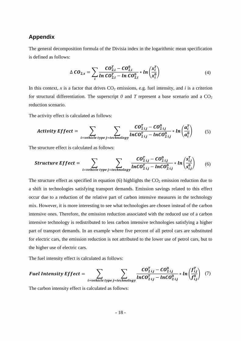
Appendix

The general decomposition formula of the Divisia index in the logarithmic mean specification

is defined as follows:

(4)

In this context, x is a factor that drives CO2 emissions, e.g. fuel intensity, and i is a criterion

for structural differentiation. The superscript 0 and T represent a base scenario and a CO2

reduction scenario.

The activity effect is calculated as follows:

(5)

The structure effect is calculated as follows:

(6)

The structure effect as specified in equation (6) highlights the CO2 emission reduction due to

a shift in technologies satisfying transport demands. Emission savings related to this effect

occur due to a reduction of the relative part of carbon intensive measures in the technology

mix. However, it is more interesting to see what technologies are chosen instead of the carbon

intensive ones. Therefore, the emission reduction associated with the reduced use of a carbon

intensive technology is redistributed to less carbon intensive technologies satisfying a higher

part of transport demands. In an example where five percent of all petrol cars are substituted

for electric cars, the emission reduction is not attributed to the lower use of petrol cars, but to

the higher use of electric cars.

The fuel intensity effect is calculated as follows:

(7)

The carbon intensity effect is calculated as follows:

- 19 -

(8)

- 20 -

References

AEA Energy & Environment (2008). Emissions of carbon dioxide, methane and nitrous oxide

by NC source catergory, fuel type and end user. London, Department for

Environment, Food and Rural Affairs.

Anandarajah, G., N. Strachan, P. Ekins, R. Kannan and N. Hughes (2008). Pathways to a Low

Carbon Economy: Energy systems and modelling. London, UKERC.

Ang, B. W. (2004). "Decomposition analysis for policymaking in energy:: which is the

preferred method?" Energy Policy 32(9): 1131-1139.

Ang, B. W. and F. Q. Zhang (2000). "A survey of index decomposition analysis in energy and

environmental studies." Energy 25(12): 1149-1176.

Ang, B. W., F. Q. Zhang and K.-H. Choi (1998). "Factorizing changes in energy and

environmental indicators through decomposition." Energy 23(6): 489-495.

Carmel, A. (2008). Paying for mitigation - The GLOCAF model. United Nations Framework

Convention on Climate Change COP 13. Bali, Indonesia.

Committee on Climate Change (2008). Building a low-carbon economy - the UK's

contribution to tackling climate change. London.

Diakoulaki, D., G. Mavrotas, D. Orkopoulos and L. Papayannakis (2006). "A bottom-up

decomposition analysis of energy-related CO2 emissions in Greece." Energy 31(14):

2638-2651.

Divisia, F. (1925). "L'indice monétaire et la théorie de la monnaie." Revue d'économie

politique 39(5): 980-1008.

Halsnaes, K., P. Shukla, D. Ahuja, G. Akumu, R. Beale, J. Edmonds, C. Gollier, A. Grübler,

M. H. Duong, A. Markandya, M. McFarland, E. Nikitina, T. Sugiyama, A.

Villavicencio and J. Zou (2007). Framing Issues. Climate Change 2007: Mitigation.

Contribution of Working Group III to the Fourth Assessment Report of the

Intergovernmental Panel on Climate Change. B. Metz, O. R. Davidson, P. R. Bosch,

R. Dave and L. A. Meyer. Cambridge, UK and New York, NY, USA, Cambridge

University Press.

Hankinson, G. A. and J. M. W. Rhys (1983). "Electricity consumption, electricity intensity

and industrial structure." Energy Economics 5(3): 146-152.

HM Government (2009). Analytical Annex - The UK Low Carbon Transition Plan. London.

Hourcade, J.-C., K. Halsnaes, M. Jaccard, W. D. Montgomery, R. Richels, J. Robinson, P.

Shukla and P. Sturm (1995). A Review of Mitigation Cost Studies. Climate Change

1995: Contribution of Working Group III to the Second Assessment of the

Intergovernmental Panel on Climate Change. J. J. Houghton, L. G. Meiro Filho, B. A.

Callanderet al. Cambridge, United Kingdom, Cambridge University Press.

Jackson, T. (1991). "Least-cost greenhouse planning supply curves for global warming

abatement." Energy Policy 19(1): 35-46.

Kannan, R., N. Strachan, N. Balta-Ozkan and S. Pye (2007). UK MARKAL model

documentation. UKERC working paper.

Kaya, Y. (1989). Impact of carbon dioxide emission control on GNP growth: interpretation of

proposed scenarios. IPCC Energy and Industry Subgroup - Response Strategies

Working Group. (mimeo). Paris.

Kesicki, F. (2010). Marginal Abatement Cost Curves for Policy Making – Expert-Based vs.

Model-Derived Curves. IAEE’s 2010 International Conference. Rio de Janeiro.

- 21 -

Loulou, R., G. Goldstein and K. Noble (2004). Documentation for the MARKAL Family of

Models, Energy Technology Systems Analysis Programme.

Montgomery, J. K. (1937). The Mathematical Problem of the Price Index. London, P.S. King

& Son, Ltd.

Naucler, T. and P. A. Enkvist (2009). Pathways to a Low-Carbon Economy - Version 2 of the

Global Greenhouse Gas Abatement Cost Curve. McKinsey & Company.

Shrestha, R. M., G. Anandarajah and M. H. Liyanage (2009). "Factors affecting CO2

emission from the power sector of selected countries in Asia and the Pacific." Energy

Policy 37(6): 2375-2384.

Strachan, N., R. Kannan and S. Pye (2008). Scenarios and Sensitivities on Long-term UK

Carbon Reductions using the UK MARKAL and MARKAL-Macro Energy System

Models. London, UKERC.

Torvanger, A. (1991). "Manufacturing sector carbon dioxide emissions in nine OECD

countries, 1973-87 : A Divisia index decomposition to changes in fuel mix, emission

coefficients, industry structure, energy intensities and international structure." Energy

Economics 13(3): 168-186.

Vartia, Y. O. (1976). "Ideal Log-Change Index Numbers." Scandinavian Journal of Statistics

3(3): 121-126.

Viguier, L. L., M. H. Babiker and J. M. Reilly (2003). "The costs of the Kyoto Protocol in the

European Union." Energy Policy 31(5): 459-481.