maptile mapping in Stata, made easy - Michael Stepnerfiles.michaelstepner.com/maptile slides 2015-03...
39
maptile mapping in Stata, made easy Michael Stepner MIT
Transcript of maptile mapping in Stata, made easy - Michael Stepnerfiles.michaelstepner.com/maptile slides 2015-03...

maptile
mapping in Stata, made easy
Michael Stepner
MIT


. maptile population, geo(state)
7.36 − 23.674.59 − 7.363.07 − 4.591.95 − 3.070.92 − 1.950.40 − 0.92

Ingredients for creating a map
. maptile population, geo(state)
1) Install maptile
The installation command is posted at:
www.michaelstepner.com/maptile/ maptile depends on the Stata program spmap
. ssc install spmap

Ingredients for creating a map
2) Install a maptile geography template
Install templates from:
www.michaelstepner.com/maptile/geographies
. maptile population, geo(state)

Ingredients for creating a map
. maptile population, geo(state)
2) Install a maptile geography template
Install templates from:
www.michaelstepner.com/maptile/geographies

Ingredients for creating a map
3) Data with a geographic ID variable

Ingredients for creating a map
3) Data with a geographic ID variable
Geographic ID in dataset must be compatible with template.

Ingredients for creating a map
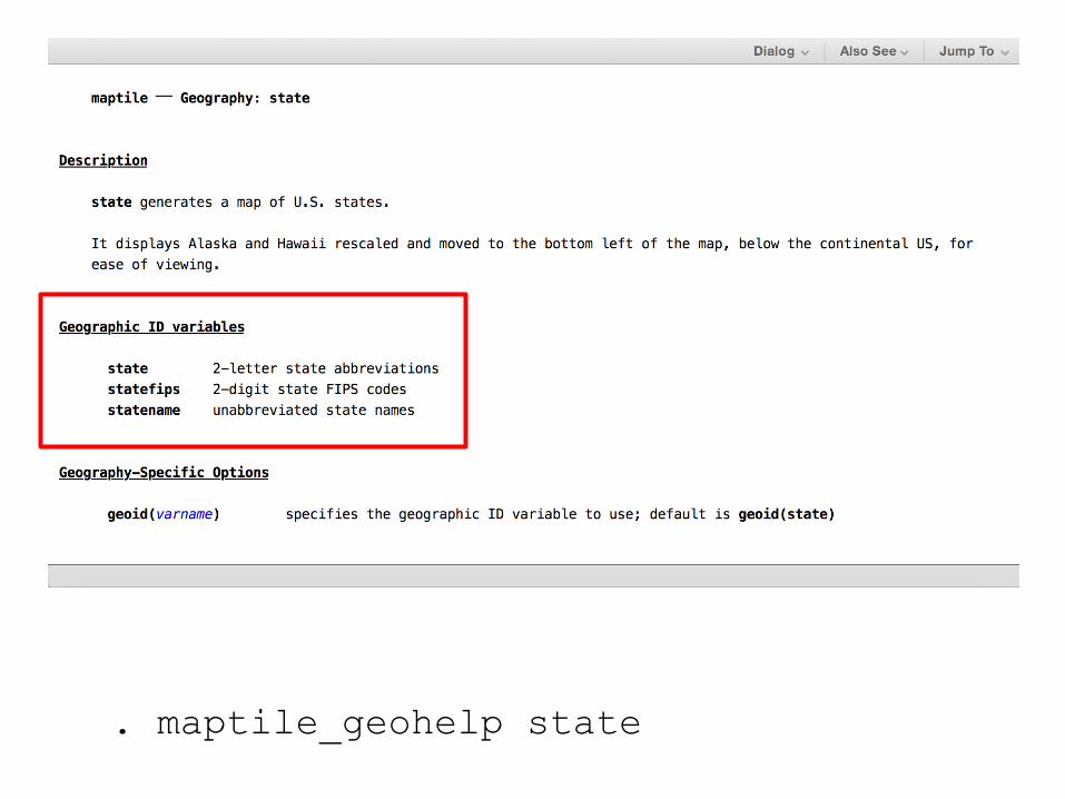
3) Data with a geographic ID variable
To learn template requirements and options, run:
. maptile_geohelp state

Making maps
“More an art than a science.”

Ingredients for creating a map
Ingredients for creating a map
. maptile_geohelp state

Ingredients for creating a map
. rename statecode statefips
. rename state statename

Ingredients for creating a map
826 − 926758 − 826729 − 758706 − 729669 − 706624 − 669
. maptile mort_white, geo(state) geoid(statefips)

What’s happening under the hood
Equal-sized bins
Same number of states in each bin (up to integer rounding)
“Equal-spaced” colors
The color assigned to each bin depends only on the bin number, not on the values of the data in the bin
N.B. Color “spacing” is not well-defined except on a fixed color spectrum.
Colors are ordinal, not cardinal

669 624 706 729 758 826 926
NJ
ND
WA
WI
AK
MD
MA
NH
RI
UT
VT
VA
IL
IA
NE
OR
NM
PA
TX
WY
DE
ID
KS
ME
MT
NV
NC
OH
SC
GA
IN
MI
MO
MS
OK
TN
WV
AL
AR
KY
LA
HI
MN
NY
SD
AZ
CA
CO
CT
FL
Q2 Q3 Q4 Q5 Q6 Q1
. xtile cutpoints_white=mort_white, nq(6)

. maptile mort_white, geo(state)
0 0.2 0.4 0.6 0.8 1
Q2 Q3 Q4 Q5 Q6 Q1
Q2 Q3 Q4 Q5 Q6 Q1
669 624 706 729 758 826 926
NJ
ND
WA
WI
AK
MD
MA
NH
RI
UT
VT
VA
IL
IA
NE
OR
NM
PA
TX
WY
DE
ID
KS
ME
MT
NV
NC
OH
SC
GA
IN
MI
MO
MS
OK
TN
WV
AL
AR
KY
LA
HI
MN
NY
SD
AZ
CA
CO
CT
FL

Ingredients for creating a map
826 − 926758 − 826729 − 758706 − 729669 − 706624 − 669
. maptile mort_white, geo(state)

Proportional color spacing: captures dispersion
Equally-spaced colors are: Informative about order Uninformative about dispersion
Can use “proportionally-spaced colors” instead: 1) Compute the median value in each bin 2) Place the lowest bin at the left, highest at the right 3) Color the middle bins proportionally to the distance
between them
à Bins containing similar values will have similar colors
N.B. There is nothing objective about color spacing.
Proportionally-spaced colors on one color spectrum are equivalent to equally-spaced colors on a different spectrum.

. maptile mort_white, geo(state)
Q2 Q3 Q4 Q5 Q6 Q1
669 624 706 729 758 826 926
100 45 37 23 29 68
0 0.2 0.4 0.6 0.8 1
Q2 Q3 Q4 Q5 Q6 Q1

. maptile mort_white, geo(state) propcolor
Q2 Q3 Q4 Q5 Q6 Q1
Q2 Q3 Q4 Q5 Q6 Q1
657 687 714 738 799 903
657 687 714 738 799 903

Ingredients for creating a map
826 − 926758 − 826729 − 758706 − 729669 − 706624 − 669
. maptile mort_white, geo(state) propcolor
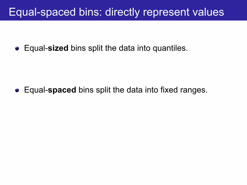
Equal-spaced bins: directly represent values
Equal-sized bins split the data into quantiles.
Equal-spaced bins split the data into fixed ranges.

Ingredients for creating a map
650 624 700 750 800 900 926
NJ
ND
WA
WI
AK
MD
MA
NH
RI
UT
VT
VA
IL
IA
NE
OR
NM
PA
TX
WY
DE
ID
KS
ME
MT
NV
NC
OH
SC
GA
IN
MI
MO
MS
OK
TN
WV
AL
AR
KY
LA
HI
MN
NY
SD
AZ
CA
CO
CT
FL
B7
669 624 706 729 758 826 926 Q2 Q3 Q4 Q5 Q6 Q1
B6 B5 B4 B3 B2 B1
850
OK WV
AL KY MS
HI MN SD
MA NH NJ NY ND WA
AK AZ CA CO CT FL MD
OR RI UT VT VA WI WY
DE ID IL IA KS MT NE NM
NC PA TX
GA ME MI MO
OH SC
IN NV TN
AR LA

Ingredients for creating a map
900 − 926850 − 900800 − 850750 − 800700 − 750650 − 700624 − 650
. maptile mort_white, geo(state) cutvalues(650(50)900)

Loops
foreach race in white black { maptile mort_`race', geo(state) /// savegraph(fig/map_mort_`race'.eps)
}
Same way you would do any loop in Stata

Ingredients for creating a map
826 − 926755 − 826729 − 755702 − 729668 − 702466 − 668
. maptile mort_white, geo(state)
White Mortality Rates

Ingredients for creating a map
967 − 1,050918 − 967805 − 918740 − 805582 − 740246 − 582
. maptile mort_black geo(state)
Black Mortality Rates

Absolute comparisons between groups
When each group uses its own bins, the map shows a relative comparison between the groups
“Where are black Americans worst off, relative to other black Americans?”
“Where are white Americans worst off, relative to other white Americans?”
An absolute comparison is also interesting:
“How do black Americans fare, relative to white Americans?”
To see this comparison, hold the bins fixed.

Absolute comparisons between groups
Generate a variable containing the break points using the distribution of white mortality:
pctile mort_white_breaks=mort_white, nq(6)
Map both white and black mortality using the same break points:
maptile mort_white, geo(state) cutp(mort_white_breaks)
maptile mort_black, geo(state) cutp(mort_white_breaks)

Ingredients for creating a map
826 − 926755 − 826729 − 755702 − 729668 − 702466 − 668
. maptile mort_white, geo(state) cutp(mort_white_breaks)
White Mortality Rates

Ingredients for creating a map
826 − 1,050755 − 826729 − 755702 − 729668 − 702246 − 668
Black Mortality Rates
. maptile mort_black, geo(state) cutp(mort_white_breaks)

Making maps
“More an art than a science.”
Data values are cardinal
Color spectrum is ordinal
à Choice of binning procedure and color spacing should depend on the features of the data that you want to highlight.

How maptile works
Data + Shapefile
spmap
maptile
Highly customizable
Template
Information
Easy to use

How maptile works
Data + Shapefile
spmap
maptile
Highly customizable Template
Information
Easy to use

Making a new template
There are detailed instructions in the maptile help file
Requires you to:
Find a shapefile for the region you want to map
Edit an ado-file that connects maptile to your shapefile
If you make a new template, consider sharing it!
Send it to me and I will post it on the maptile website with your name.
With your help, people will be able to quickly make maps of many different places.

Making a new template
Useful resources:
demo_maptile.ado (linked from the help file) provides a base and a step-by-step guide to each line of code you need to edit.
Download the “Creation Files” for any template posted on the maptile website to see how the shapefile was processed.
To copy a feature from an existing template, download the template’s zip file and look at the code in the ado-file.
(Instead of copying and pasting the maptile_install command into Stata, copy and paste the URL in your browser.)

. maptile median_income, geo(can_prov)

Making maps?
No problem.