Mapping relation algebra operators into SQL queries: A … · · 2015-07-17Mapping relation...

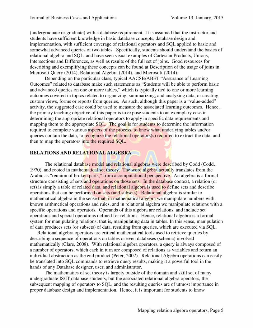
Journal of Business Cases and Applications Volume 13, January, 2015

Mapping relation algebra operators,

Mapping relation algebra operators into SQL queries: A database

case study

John N. Dyer

Georgia Southern University

Camille Rogers Georgia Southern University

ABSTRACT

Relational algebra operators and mapping to resulting structured query language (SQL) queries are among the most important concepts and skills for students taking a course in database design and implementation, especially those majoring in IS/IT. The most typical relational algebra operators mapped to foundational SQL include unions and intersections, as well as other relational operators applied to these operators, including differences and various joins. Unfortunately, few textbooks or external resources provide ample opportunity for students to apply the full set of most common relational algebra operators mapped to resulting SQL over a single unified case. Most database textbooks exemplify each separate relational algebra construct to a single, sparse (although visually-stimulating) example, wherein the full set of operators is not near fully exemplified. This paper presents an overview of a case example that exemplifies and maps a more complete set of relational algebra operators in related SQL operations across a unified case. The case replicates the author’s real experience in building a database solution for an online retailer of sporting goods products. It is hoped that this case example will help database teachers more effectively teach relational algebra concepts, the subsequent mapping to SQL, and resulting queries, as well as provide students a greater understanding of relational algebra and mapping to SQL. Although the case example is exemplified in Microsoft Access 2010/2013, the case can be modified and presented using any relational database management system (RDBMS). Keywords: Relational Algebra, Relational Operators, SQL, Database Case Study Copyright statement: Authors retain the copyright to the manuscripts published in AABRI journals. Please see the AABRI Copyright Policy at http://www.aabri.com/copyright.html



CASE OVERVIEW

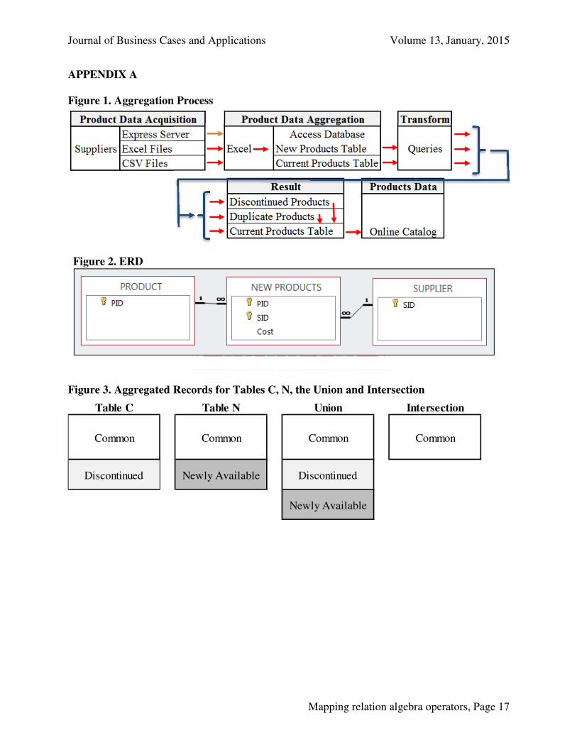
F&B Trader’s is a small online wholesaler of food and beverage products. The company is a pre-seller, meaning they do not stock actual inventory. Instead, they aggregate available products from various suppliers and display those products for sale in their online catalog. This practice has become very common place with both auction sellers and web-only sellers, purchasing products from suppliers only when they receive their own customer’s order, and often having the products drop-shipped by the supplier to the customer. The student works in the Purchasing & Sales Department, and among the duties is creating and running a series of queries to update the online catalog and produce reports regarding product availability. Since product inventory and costs change frequently throughout the day, the sales department must also frequently update the online catalog, every few hours throughout each day. Figure 1 (Appendix A) displays the process of aggregating supplier product availability data to creating a final catalog to display to customers online, as described below.

The company has many suppliers, and the purchasing agent aggregates available products frequently from all suppliers throughout the day. Some suppliers provide web services directly to F&B using Microsoft Express Server, which updates product availability in real-time onto F&B’s PC, while other suppliers provide downloadable Excel and CSV product files from their website. The purchasing agent has an Excel VBA program that extracts and combines all products available from all suppliers that are in the Express Server database, as well as the Excel and CSV files, and then imports it into the Access database tables. Some products are available from only a single supplier, while other products are available from multiple suppliers, sometimes at the same or even different costs. The purchasing agent aggregates the changing product list frequently, which shows all products most recently available from all suppliers. That is, it is the most recently aggregated list of available products and prices.

Note, the most recent aggregated table may have newly available products that are not in the current online catalog, or, it may exclude products that are no longer available (but still shown in the current online catalog), and some costs may have changed for existing products since the last update. Although the aggregated table can contain the same product(s) available from different suppliers (duplicate products) at the same or different costs, the online catalog can display the duplicate products only once, and at the lowest cost available. That is, if the same product is available from three suppliers at three different costs, the next online catalog must show it available only once, and at the lowest cost. Likewise, if two suppliers provide the same product at the same price, the online catalog must show the product only once. Otherwise, an online customer who searches the catalog would wonder why the same product is listed multiple times at different costs. Additionally, the online catalog doesn’t display the supplier, only the product ID and their cost, along with other non-key attributes like description, quantity available, etc.

The F&B database contains two primary tables; Product and Supplier, with key attributes of Product ID (PID), Supplier ID (SID), and Cost, respectively. Additionally, the business rules are such that a supplier can supply many products, and a product can be supplied by many suppliers, hence a many-to-many relationship. Furthermore, a supplier does not have to supply any products at any given time, a specific product may or may not be available at any given time, but multiple suppliers may often supply the same product at the same or different costs. As such, the many-to-many relationship is bridged using the New Products table, related through attributes PID and SID, and the additional Cost attribute. The ERD is shown in Figure 2



(Appendix A), omitting non-key attributes from the tables. Only the 3 key attributes of PID, SID and Cost are used in this case.

So, at any given time, F&B has two primary Access database tables; the Current Products table (the latest uploaded online catalog) and the New Products table (the most recently aggregated list from the purchasing agent). The sales agent must then be able transform the New Products table to next Current Products table (using various queries), to come up with products to upload to the website every few hours. Hence, he must include the newly available product/supplier/cost combination records, and remove duplicate products available from multiple suppliers, leaving only one duplicate product that has the lowest cost. If duplicate products are available from two or more suppliers at the same lowest cost, he only wants to display one duplicate, and it doesn’t matter which one. Additionally, F&B would like to retain data regarding which product/supplier/cost combinations are not currently available (discontinued product/supplier/cost records from the last online catalog to the most recent), newly available product/supplier/cost records (not in the last online catalog), as well as duplicate products that are available from multiple suppliers.

So, the following summary tasks are at hand to create the next Current Product table from the New Products table, and to provide the following information.

• Product/supplier/cost combinations (records) that are no longer included in the next Current Products table.

• Newly available product/supplier/cost combinations (records) that have been added since the last update, and thus need to be included in the next online catalog.

• Duplicate products available from different suppliers at equal and/or different costs shown in the New Products table.

• The new Current Products table showing the existing and new products, but removing duplicate products, thus leaving only the lowest cost duplicate of each duplicate product.

This can be viewed as a continuously repeated information processing cycle of

1) Input: Gather inputs from the

• Current Products table (currently listed online)

• New Products table (recently aggregated by purchasing) 2) Processing: Process the inputs using queries for the Union, Intersection,

Differences, and other specialized queries.

3) Output: • The list of discontinued (no longer available) products.

• The list of newly available products.

• The list of duplicate products showing the products, suppliers and costs.

• The list of final products that are to be uploaded to the next online catalog.

4) Storage: Store each output as a table or query in the database.

5) Communication: Upload the new list of final products to the online catalog, which is now the newest (or next) Current Products table in the database.

To perform these tasks, the student must recognize and map the necessary relational algebra operators between tables and queries (using various joins), to ultimately produce the next Current Products table for the sales agent to upload onto the website.



INTRODUCTION

Most modern database textbooks cover various topics in basic database concepts, followed by the design, implementation, and management of relational database management systems (DBMS). Design aspects typically relate to design concepts, relational algebra and set operators, relationship types, the entity relationship model, entity integrity, normalization, and relationship integrity. Implementation aspects relate primarily to SQL, including data definition commands, data manipulation commands, select queries, and various joins. Management aspects typically relate to transaction management, concurrency control, performance and optimization, distributed DBMS, data warehousing and business intelligence.

While the textbooks are somewhat sparse in coverage of mapping relational algebra operators to SQL, and resulting query results, the pedagogical literature is very sparse in all regards to database design, implementation and management. In fact, since 2004, only 8 articles have appeared in The Journal of Information Systems Education regarding database. Of these, 2 are teaching cases (Green, 2005) (Irwin, Wessel and Blackburn, 2012), while 6 cover topics loosely related to teaching various database concepts (Itri, 2012), (Casterella and Vijayasarathy, 2013), (Unch, 2009), (Carpenter, 2008), (Olsen and Hauser, 2007), and (Hsiang-Jui and Hui-Lien, 2006)

In many cases the concepts of relational algebra (as it relates to relational set operators) are presented to students as design aspects, but not fully exemplified in later implementations via SQL mappings. That is, a student may never realize that a set difference described in design concepts can be mapped to an SQL outer join operation in implementation, or an intersection can be mapped to either an SQL outer or inner join. The concepts of relational operators are largely demonstrated visually using sparse examples of a Cartesian Product (X), Union (U), Union All (UA), Intersection (I), Difference (D), and Division (%). Later, in implementation of SQL, the relational operators are not discussed in terms of the associated SQL and the various joins which produce the queries represented by the relational operators.

This paper presents an overview of a case example that exemplifies and maps nearly the entire set of relational algebra operators in related join operations across a unified case. It is hoped that this case example will help database teachers more effectively teach relational algebra concepts, SQL and resulting queries, as well as provide students a greater understanding of relational algebra operators and the subsequent mapping to SQL. Although the case example is exemplified in Microsoft Access 2010/2013, the case can be modified and presented using any relational database management system (RDBMS). Access is used as an exemplary DBMS to mimic an enterprise DBMS, with the added advantage of concept and design visualization, student familiarity, ready availability, and ease of design, implementation and management. To fully exemplify this case example, the instructor and students are expected to have familiarity with Access 2010/2013, specifically the query tools including the Query Wizard, Query Design View (using the Query by Example Design Grid (QBE)), and the SQL View.

Many students in programs in information systems (IS), information technology (IT), or computer science (CS) are required to take an introductory database course which includes many of the topics discussed above. Different programs may focus on more specific aspects, like IS focus on design and basic implementation, an IT focus on hardware/software management, or a CS focus on relational algebra/calculus, advanced SQL and SQL optimization. What most programs do have in common is the SQL component, regardless of the degree to which it is exemplified. As such, this paper is directed toward students majoring in IS/IT/CS



(undergraduate or graduate) with a database requirement. It is assumed that the instructor and students have sufficient knowledge in basic database concepts, database design and implementation, with sufficient coverage of relational operators and SQL applied to basic and somewhat advanced queries of two tables. Specifically, students should understand the basics of relational algebra and SQL, and have seen visual examples of Cartesian Products, Unions, Intersections and Differences, as well as results of the full set of joins. Good resources for describing and exemplifying these concepts can be found at Description of the usage of joins in Microsoft Query (2014), Relational Algebra (2014), and Microsoft (2014).

Depending on the particular class, typical AACSB/ABET “Assurance of Learning Outcomes” related to database make such statements as “Students will be able to perform basic and advanced queries on one or more tables,” which is typically tied to one or more learning outcomes covered in topics related to organizing, summarizing, and analyzing data, or creating custom views, forms or reports from queries. As such, although this paper is a “value-added” activity, the suggested case could be used to measure the associated learning outcomes. Hence, the primary teaching objective of this paper is to expose students to an exemplary case in determining the appropriate relational operators to apply in specific data requirements and mapping them to the appropriate SQL. The goal is for students to determine the information required to complete various aspects of the process, to know what underlying tables and/or queries contain the data, to recognize the relational operators(s) required to extract the data, and then to map the operators into the required SQL.

RELATIONS AND RELATIONAL ALGEBRA

The relational database model and relational algebras were described by Codd (Codd, 1970), and rooted in mathematical set theory. The word algebra actually translates from the Arabic as “reunion of broken parts,” from a computational perspective. An algebra is a formal structure consisting of sets and operations on those sets. In the database context, a relation (or set) is simply a table of related data, and relational algebra is used to define sets and describe operations that can be performed on sets (and subsets). Relational algebra is similar to mathematical algebra in the sense that, in mathematical algebra we manipulate numbers with known arithmetical operations and rules, and in relational algebra we manipulate relations with a specific operations and operators. Operands of this algebra are relations, and include set operations and special operations defined for relations. Hence, relational algebra is a formal system for manipulating relations; that is, manipulating data in tables. In this sense, manipulation of data produces sets (or subsets) of data, resulting from queries, which are executed via SQL.

Relational algebra operators are critical mathematical tools used to retrieve queries by describing a sequence of operations on tables or even databases (schema) involved mathematically (Clare, 2008). With relational algebra operators, a query is always composed of a number of operators, which each in turn are composed of relations as variables and return an individual abstraction as the end product (Peter, 2002). Relational Algebra operations can easily be translated into SQL commands to retrieve query results, making it a powerful tool in the hands of any Database designer, user, and administrator.

The mathematics of set theory is largely outside of the domain and skill set of many undergraduate IS/IT database students, but the associated relational algebra operators, the subsequent mapping of operators to SQL, and the resulting queries are of utmost importance in proper database design and implementation. Hence, it is important for students to know



relational algebra to better understand query execution, and to a lesser extent, query optimization. See Mivule (2014) for a more extensive treatment.

Terminology and notation related to database can differ significantly across the IS/IT/CS disciplines, from friendlier applied “laymen’s” terms to the complex functional notation in relational calculus. Although there are strict definitions used to describe components of a database, we will establish in this paper that that a relation is a table or query, an attribute is a field or column in a table or query, and that a tuple is a record or row. Hence, a table (or query) is a collection of data pertaining to related records, the data being stored in a structured format, made up of attributes describing various characteristics of each record. A cell in a table can be described as storing data regarding the attribute value for a specific record. Regarding notation, we will tend more to the applied style so as to avoid functional notation complexity, which can be off-putting to those with a limited math background.

The five primary relational algebra operators as defined by Codd include SELECT (σ), PROJECT (π), and the previously defined operators X, U, and D. Although Codd did not include I as a primary operator (as it is formally defined in terms of D), we will include it as a primary operator. The interested reader should see Connolly, T., & Beg, C. (2010), and Mannino (2014) for a more discussive treatment of operations in relational algebra, including operation, notation, and function. Each of the above operators, with the exception of σ and π, are used to create joins, which combine records from two or more relations. While σ and π can relate to one or more relations, the other operators always relate to two or more relations, like tables A and B. We will not explicitly apply X in this case, as it is simply a conceptual DBMS internal procedure facilitating various joins to be performed. That is, a join ⊕ of two tables, like A⊕B, first requires X, and then selection (σ) of desired records, and then projection (π) of the desired attributes for the resulting records. When relations are joined, selection is usually based on a predicate, which can be thought of as a condition on which records are included or excluded from a set. In most cases, the join is based on matching on a common attribute (or attributes) in both relations, usually the primary key (PK) of table A being shared as the foreign-key (FK) in table B, also known as a PK-FK relationship. It should be noted that while X does have importance in other applications outside the scope of this case. It should also be noted that the relational operator % is also formally expressed in terms of D, hence not a primary operator, and outside of the scope of this case.

It is important to recall that σ relates to selecting (retrieving) records, while π relates to projecting (displaying) attributes. One should be aware that these operators always select and project from a single view. A view is a dynamic representation of a single relation, or from two or more joined relations, specified in a FROM clause. For two or more relations, a join is performed on one or more common attributes (columns) using the ON clause (with our without a predicate). Hence, a view is also considered a relation. Although σ proceeds the FROM and ON clauses in SQL, these two clauses are actually executed first.

Additionally, σ is both the most important operator and SQL clause, and is always used to express a query. It combines the three fundamental relational algebra operations; ⊕, σ, and π. Every σ clause produces a query consisting of one or more attributes and zero or more records. The σ clause must have the corresponding tables, queries or views specified in the FROM clause. In the case of A⊕B, the ON clause must specify the common matching attribute(s) in tables A and B. The WHERE clause selects the subset of records to be included in the query by applying a search condition (a predicate) to the records of the specified table(s).



Different DBMSs may or may not support a specific implementation of an operator. For example, Oracle supports the X operator with the CROSS JOIN clause, the I operator with the INTERSECT clause, and the D operator with the MINUS clause. In Access 2013, X is implemented as a simple SELECT * FROM two tables with a full projection of all attributes, I is implemented as either an outer join with predicates or an inner join (IJ), while D is implemented as either a left outer join (LJ) or right outer join (RJ) on a common attribute(s) with predicates. The MINUS operator in Oracle requires both tables to be union-compatible, while outer joins do not. In any case, all DBMSs require U, I and D operators be performed on union-compatible tables.

STRUCTURED QUERY LANGUAGE – SQL

SQL is a special purpose programming language designed for managing and querying data in a RDBMS. Relational algebra operators are translated into SQL commands to query records and summarize data from tables in a database. SQL can be described as a declarative language (in contrast to a procedural language), wherein declarative programming describes what should be done but not how to do it. At lower level operations within a DBMS, the SQL is translated into procedures based on relational algebra constructs. That is, the relational algebra operations are executed according to the explicit SQL statements, and are done so by executing programs inside a DBMS’s inner-workings using a procedural language. SQL can be typed and executed from a terminal-type screen within the DBMS, or can be embedded in a procedural language.

To more fully understand the difference (applied to a more typical algebra problem), one might find the square-root of 64 using a calculator. The user inputs the number 64 and presses the square-root button; much like one writes an SQL statement. The user is saying “calculate the square-root of 64,” but does not specify how it is to be done. The inner-workings of the calculator (using a procedural language) then translate the request into the actual operations necessary to calculate the answer, and then returns the answer 8.

SQL can be divided into two separate languages; A data definition language (DDL) versus a data manipulation language (DML). DDL includes statements for creating and modifying the schema of a database by adding, changing and deleting tables, views, and objects, as well as specifying field data-types and constraints, and defining referential integrity relationships via primary-key (PK) and foreign-key (FK) relationships. Common DDL SQL statements include CREATE, DROP, ALTER, wherein the tables and objects are defined and managed.

DML is used to retrieve, manipulate, modify and manage data in the RDBMS. Common DML SQL clauses include SELECT, INSERT, UPDATE, DELETE. Associated keywords (which are reserved) include *, DISTINCT, FIRST, LAST, AS, FROM, WHERE, GROUP BY, HAVING, and ORDER BY. Keywords for various joins include UNION, UNION ALL, INNER JOIN, LEFT JOIN, and RIGHT JOIN, where the join fields are specified with the keyword ON. ORACLE and MS SQLServer also include joins clauses such as INTERSECT, CROSS JOIN, MINUS, and EXCEPT. It should be noted that SQL search conditions (predicates) are typically specified by the WHERE clause, and in cases of creating frequency distributions or calculating aggregate functions, the use of the GROUP BY and HAVING clauses (Taylor, 2014).

These search conditions are typically restrictions on selected records. As such, SQL facilitates data manipulation through the use of predicates (or predicate expressions) following



the search clauses. The predicates can use additional logical operators including AND, OR, LIKE, IN, BETWEEN, EXISTS, NOT, IS NULL, IS NOT NULL, EXISTS, and DISTINCT,

and various equality and inequality comparison operators (<, ≤, <>, >, ≥, =). Additionally, the logical operators AND, OR, and NOT are used to combine two or more predicates into one. Aggregate functions can be used to summarize query results and include FIRST, LAST, COUNT, SUM, AVERAGE, MAX, and MIN, among others. The common arithmetic operators include +, -, *, and /. The WHERE clause cannot be used with aggregate functions. Instead, the HAVING clause follows the GROUP BY clause to restrict groups of returned records to only those whose aggregate predicate condition is true. DML SQL statements are used to embed the relational algebra constructs required to query data from a table, or two or more related tables. Although all modern enterprise DBMSs support the most common DML statements, many use different syntax, and some have included additional DBMS specific custom DML statements. For more exemplary discussions see Taylor (2014), SQL Tutorial (2014), and Tutorials Point - Simply Easy Learning (2014).

MAPPING RELATIONAL OPERATORS TO JOINS

Queries are developed by first determining what information is to be derived from a query, the underlying tables storing the data, the type of relational operator(s) required to extract the data, then mapping the relation operators to various joins available in DML. As such, it is critical to define the result set of relational algebra operators on two tables and determine the mapping to SQL statements and clauses, including affected tables, records to be queried by join type and related predicates, and appropriate projection. As such, the relational operators are provided below, including the Union, Union All, Intersection and Difference. Note that all the operators below require two tables (A and B) to be union compatible.

Union (U) Every record in A alone, in B alone, and records shared by both (i.e., the intersection). The union removes duplicate records found in A and B.

Union All (UA) Every record in A alone, in B alone, and records shared by both (i.e., the intersection), including duplicate records from A and B.

Intersection (I) Only the common records shared in table A and table B.

Difference (D) Those records in one table which are not also records in the other table.

The Difference (D) can then be more fully defined in terms of database tables A and B as

follows, wherein we call A the left table and B the right table.

D(A-B)

The difference of A and B contains those records in A which are not also records in B. The result A-B is obtained by taking A and removing from it those records which are also found (matched) in B.

D(B-A)

The difference of B and A contains those records in B which are not also records in A. The result B-A is obtained by taking B and removing from it those records which are also found (matched) in A.

Again, while Access does not implement an SQL clause for either I or D, the operators

are employed in this case using inner and outer joins (with predicate). Note that much of the data is often lost when applying a join to two tables. In some cases this lost data might hold



useful information. An outer join (left or right) retains the information that would have been lost from the tables, replacing missing data with nulls. Outer joins in and of themselves may not necessarily be useful, but when conditioned on predicates they yield quite useful information (Relational Algebra, 2008). The two primary outer joins and the inner join then are defined below.

Left Outer Join (LJ) All the records in A, with and without matches in B.

Right Outer Join (RJ) All the records in B, with and without matches in A.

Inner Join (IJ) All the records in A with a match in B.

Additionally, to find D using outer joins LJ and RJ, and I using IJ, two new predicate

terms are introduced in this paper; Excluding and Including, as defined below. Note that these predicate terms are neither introduced nor defined in database textbooks or literature but are required to map differences to outer joins.

Excluding (E)

Regarding LJ, excluding implies a predicate that excludes records from A that are null (not matched) in B; notation LJ(E). The predicate is a WHERE clause with an Is Null condition on a key attribute in B. Vice-versa for RJ, notation RJ(E).

Including (I)

Regarding LJ, including implies a predicate that includes records from A that are not null (matched) in B; notation LJ(I). The predicate is a WHERE clause with an Is Not Null condition on a key attribute in B. Vice-versa for a RJ, notation RJ(I).

As such, LJ(E) maps the D(A-B) relational operator to the SQL left join clause with the

excluding predicate, while RJ(E) maps the D(B-A) relational operator to the SQL right join clause with the excluding predicate. Additionally, both the LJ(I) or RJ(I) maps the I relational operator to the SQL left join or right join clause with the including predicate. This means that every D and I operator can be written as an outer join, but every outer join does not result in a D or I. Hence, the following equalities are newly defined;

D(A-B) = LJ(E) D(B-A) = RJ(E) I = LJ(I) = RJ(I)

It should also be noted that although I is formally defined in terms of a D (proof and

example omitted), I results from an IJ matching on all attributes, so that I = IJ = LJ(I) = RJ(I). That is, every I operator can also be written as an inner join matching on all attributes, but not every inner join results in an I. In practice, an IJ is typically used to find I since it is generally faster than outer joins with predicates.



GENERIC SQL FOR JOINS

Equally important to mapping relational operators to joins is writing the SQL statements that produce the desired queries. Most textbooks and examples demonstrate relational algebra operators/operations and SQL relative to two tables resulting from the normalization process and related through a PK-FK relationship. In other words, most examples use two tables representing different entities or record sets (each subject specific unto itself), hence related only through one common attribute. The case exemplified in this paper is unique in that all tables are of identical structure, sharing the same attributes and domains, and differ only by records; hence they are all union compatible. In essence, they are the same tables but with different records.

Table 1 (Appendix B) provides the generic SQL statements used in Access 2010/2013 to be used in this case for creating the joins discussed in the previous section. Again, let tables A and B be union-compatible. The bold words in Table 1 are SQL reserved words, those in italics indicate specific table names and/or attributes, while * refers to all attributes. When * is used to indicate projecting all attributes from a specified table, the notation A.* means “projects all attributes from table A.” When * is used below to indicate matching on all attributes from tables A and B, it follows the ON clause using notation {*}. For example, if tables A and B had two attributes, a1 and a2, and we want to match on both attributes, then {*} would formally be written in SQL as A.a1 = B.a1 AND A.a2 = B.a2, where the = and the AND operators are reserved words. Also see Steele (2014) and Relational Algebra (1998).

INSTRUCTIONAL OVERVIEW

Since the primary goal of the case example is for students to recognize and map relational algebra operators to SQL queries (using various joins) to provide a real-world business solution, it is imperative that the students understand the objectives described in the Introduction section, and the joins from the mapping section, specifically the result set obtained from U, I, and D, and that I maps to both inner joins and outer joins, while D maps to left and right outer joins (using including and excluding predicates). Also of importance are the additional specialized queries (finding duplicates and self-joins) and result sets described in Tables 2 and 3 (Appendix B). Additionally, Appendix C contains teaching notes to include teaching suggestions and an additional comprehensive student exercise. A separate set of teaching notes, the Access 2013 F&B database, and the student exercise Access database (Products) is available from the author by request.

After describing the case overview and major content of this paper with the students, the students are lead through a visual demonstration and discussion of the major steps, queries and results described in, and shown in the section below; Visual Demonstration. Table 3 supports Table 2 by enumerating each step and query, referencing the desired result, the required operator, the join type, the tables or queries used, the joined fields, the predicate (WHERE) condition applied, and the attributes to be projected. Table 4 (Appendix B) reflects the SQL required for each query in Tables 2 and 3.

To better understand Table 3, consider Step 2.A, Query Q3. The desired result is to find the records common to database tables C and N, as shown under the “Result” column. The relational operator is an intersection (I), the join type is an inner join (IJ), the tables involved are C and N, the join is on all attributes (*), and the projection is all attributes in table C (C.*). Similarly, consider Step 3.A, Query Q8. The desired result is to find the discontinued records, that is, those



records in table C that are not in table N. The relational operator is a difference (D), the join type is left join excluding (LJ(I)), the tables involved are C and N, the join is on all attributes (*), the predicate condition is where the attribute PID in table N is null (N.PID(E)), and the projection of all attributes in table C (C.*).

Footnotes are at the bottom of Table 3 describing the various asterisks shown in the table, while “na” means “not applicable.” For example, Step 5 uses a specialized query (*****) instead of a join, hence both the join type and join on columns reflect “na.” Additionally, while Table 4 (Appendix B) reflects the SQL for each step, screen-shots for each step using the Access Query by Example (QBE) grid are available from the author by request.

Note that some steps in Tables 2 and 3 are optional, showing alternative methods to achieve the same results. As such, the case can be exemplified using only the required steps and queries, while the optional steps can be used for additional “value-added” activities. Additionally, depending on the rigor of the exercise and information provided to students, either all, part, or none (or edited versions) of Tables 2, 3 and 4 may be provided to the students. Additionally, screen-shots illustrating use of the Access query design grid that can be used in lieu of writing SQL is available from the author by request.

VISUAL DEMONSTRATION

The students are provided an Access 2010/2013 database named “F&B” containing the

two tables for the case, where table C is the Current Products and table N is the New Products table. Note that there are no PKs defined, as this is not required for the exercise. One must bear in mind that when starting the cycle, although table C is currently listed online, it will be replaced following the cycle, with a new table C (i.e., final products). So, table C contains both the records that are unique to C (the discontinued product/supplier/cost combination records no longer found in N), and the records that are common to both C and N (the intersection). Similarly, table N contains both the records that are unique to only N (newly available product/supplier/cost combination records not previously found in C) and the records that are common to C and N. In general then, C contains common products (also available in N) and discontinued products, while N also contains common products, and new products.

It is also important to realize that the word “discontinued” does not imply that a particular product is no longer available from the specific supplier; only that the specific combination of PID/SID/Cost is a record in table C that is not a record in table N. It could be that the same product is still available from the same supplier but at a different cost, or that the same product is still available, but from a different supplier at the same or different cost. Likewise, the phrase “newly available” does not imply a particular product is now available that previously was not available; only that the specific combination of PID/SID/Cost is a record in table N that is not a record in table C. It could be that it is an entirely new product from an existing or new supplier, or that the specific combination of PID/SID/Cost is not a record in table C.

The aggregated and individual records of products in tables C and N, and U and I are shown in Figures 3 and 4 (Appendix A), respectively. Both U and I correspond to Q1 and Q3, respectively, in Tables 2 and 3. Note that the unshaded rows in U correspond to the intersection, the lightly shaded rows in table C and U correspond to the records only in table C (3 discontinued), while the darker shaded rows in tables N and U correspond to the records only in table N (8 newly available). In essence, these figures provide a visual solution to Q1 through Q13 in Tables 2 and 3, with the exception of Q2; Union All.



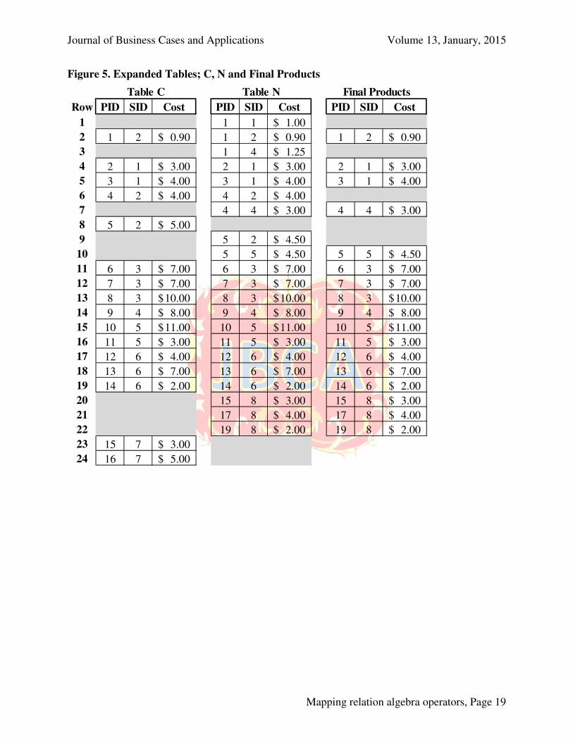
Additional discussion is provided regarding specific records in the tables, in hopes of clearly defining the record sets that will make up all required queries. Expanding the tables as in Figure 5 (Appendix A), and using row number references we can observe the following in Table 5 (Appendix B). It is suggested that students carefully study the records in each table or query, and experiment with forming IJs, OJs, and Ds related to tables C and N, as well as U and I, and other combinations of tables and queries. It is often more clear to first visualize results and then create various joins, than to start by following explicit instructions on required joins of specific tables or queries. More is often garnered by curiously viewing the results of random (but logical) joins than from trying only to decipher the question and formulate the appropriate query. Prior to demonstrating all remaining tasks, Figure 6 (Appendix A) is provided to reflect the solution (query results) for Q14 through Q21, Tables 2 and 3.

Since the first real task beyond finding U is that of finding I (Table 2 and 3, Step 2.A, Q3), students should see the actual connections between the 2 database tables. This can be done by asking, “what records do both tables have exactly in common?’ The word “exactly” is important, in that each record must match on all key attributes; PID, SID and Cost. Figure 7 (Appendix A) reflects drawing lines from C to N on matching records (although truncated for space). The shaded records in either of tables C or N will not connect, since neither is matched in the other table. One can then refer to previous sections to determine that an IJ, matching on all attributes, maps to I.

Similarly, consider Table 2 and 3, Step 3.A, Q8, the result being to find the discontinued products. In laymen’s terms, this is every record in table C that does not have not have a matching record in table N. By definition then, this is a difference between the two tables; D(C-N). The SQL for finding D(C-N) is shown from a previous section as a left join excluding, LJ(E). The two tables C and N are then left joined on all common attributes (PID, SID and Cost), with the predicate (WHERE) that only those records be returned from table C with a null value found in table N’s PID attribute.

Figure 8 (Appendix A) displays a left join of tables C and N, projecting all attributes from C (left) and N (right). It is clear to see that the 3 null records in table N (darkly shaded) correspond to the records in table C without a match in table N, meaning the records are not found in table N, hence they are a discontinuation of an exact combination of a PID/SID/Cost combination record. Notice also that only one attribute in table N need be null, instead of all 3 attributes. This is because, if the PID attribute is null in table N, then the SID and Cost attributes will also be null. We need only specify one null attribute, hence avoiding excessive and unnecessary SQL. Lastly, the query projects all attributes from only table C; none from table N.

Likewise, those PID/SID/Cost combination records in table C that are exactly matched on all attributes in table N (not null) represent the intersection (I) of tables C and N, that is, the common records (Tables 2 and 3, Step 2B*, Q4). Again, as previously defined, I=LJ(I), that is, a left join including. Recall though, an IJ on all attributes is a more efficient method of finding I.

Figure 9 (Appendix A) displays a right join of tables N and C, projecting all attributes from N (right) and C (left). Similar to Figure 8, it is clear to see that the 7 null records in table C (darkly shaded) correspond to the records in table N without a match in table C, meaning the records are not found in table C, hence they are the addition of exact combinations of a PID/SID/Cost combination record (newly available).

Again, the resulting query only projects all attributes from table N; none from table C. Likewise, those PID/SID/Cost combination records in table N that are exactly matched on all attributes in table C (not null) represent the intersection (I) of tables C and N, that is, the



common records (Tables 2 and 3, Step 2C*, Q5). Again, as previously defined, I=RJ(I), that is, a right join including.

The first specialized query (Tables 2 and 3, Step 5, Q14) is to find all duplicate products, that is, the same products supplied by multiply suppliers. Note that this is not the same as duplicate records. While duplicate records might exist in database tables C and N, with the same PID/SID/Cost, duplicate products exist in table N (as well as in the U and I), but with different SIDs. Again, for any given duplicate product, it might be available from 2 or more suppliers, at the same cost, equal cost, or higher cost, depending on the supplier. Figure 6 (Q14) displays the list of duplicate products, while the exact nature of the duplicate products is discussed in Table 3. Although this is a nested subquery query, it can be visualized by starting with table N, and grouping by those records with duplicate PIDs; that is, those records with PIDs having a Count >1. This results in a list of duplicate PIDs as shown below in Figure 10 (Appendix A), which results from a standard GROUP BY – HAVING subquery. Once the list of duplicate PIDs has been created, a standard query is used to select only those records from table N whose PID is IN (keyword) the list, and projecting all attributes. Recall, the IN clause is followed by a list of attribute values for which a match mat exist, and in this case the list is generated from the GROUP BY – HAVING subquery. So, the outer SELECT query uses the WHERE operator to search for records in table N where the PID is in the subquery list, resulting in the duplicate product records.

Once the duplicate products are found, Tables 2 and 3 Step 6 requires another specialized query to extract the high cost duplicate products from Q14 (see Figure 6, Q15). This query is an IJ (employed as a self-join) of the duplicate products query (Q14) on itself (Q14B), with a WHERE predicate to select records from Q14 whose Cost attribute value is greater than those values in Q14B. In laymen’s terms, we’re asking, “for each distinct PID in Q14, which records have a higher cost than the cost with the same PIDs in Q14B?” Figure 11 (Appendix A) reflects a visual demonstration of comparing cost in each row in Q14 with each row in Q14 where the PID matches, as discussed below. Note that all the rows of comparison in Figure 11 that have comparison resulting in “greater than” will be included in the high cost duplicate products query, which are records in rows 1, 3, and 4;

1. Compare the first row cost in Q14 with the second and third row costs in Q14B, which

results in the record being a high cost duplicate product, since it is greater than the cost in second row in Q14B.

2. Compare the second row cost in Q14 with the first and third 3 row costs in Q14B, which is not higher than either of the 2 rows, so not a high cost duplicate product.

3. Compare the third row cost in Q14 with the first 2 rows costs in Q14B, which results in the record also being a high cost duplicate product, since it is greater than the costs in both the first 2 rows.

4. Compare the forth row cost in Q14 with fifth row cost in Q14B, which results in the record being a high cost duplicate product, since it is greater than the cost in the fifth row in Q14B.

5. Compare the fifth row cost in Q14 with forth row cost in Q14B, which is not higher, so not a high cost duplicate product.

6. Compare the sixth row cost in Q14 with seventh row cost in Q14B, which is equal cost, so not a high cost duplicate product.

7. Compare the seventh row cost in Q14 with sixth row cost in Q14B, which again is equal cost, so not a high cost duplicate product.



Tables 2 and 3, Steps 7 through 12, then again use the D operator mapped to various LJ(E) and RJ(E), applied to the different queries to produce the final products query. For example, Step 7 requires finding the lower and equal cost duplicate products (Q16). Since all duplicate products are in Q14, and the high cost duplicate products are in Q15, then this is all the duplicate products in Q14 that are not in Q15. By definition, this is D(Q14-Q15), which is a LJ(E), matching on all attributes, projecting all attributes from Q14. Likewise, Step 8 requires finding only the equal cost duplicate products (Q17). This is simply a modification of Q16, but matching only on PID. Step 9 requires finding only one each of the equal cost duplicate products (Q18), and is a slight modification of Q17, using the aggregate keyword FIRST to return only the first record for each distinct PID in Q17. Step 10 requires finding the preferred duplicate products (Q19), which is every record in Q16 that is not in Q18; D(Q16-Q18), which is a LJ(E), matching only on PID, and projecting all attributes from Q16. Step 11 requires finding the duplicate products to remove, that is, those duplicate products in Q14 (all duplicate products) that are not Q19 (preferred duplicate products; D(Q14-Q19), which is a LJ(E), matching only on all attributes, and projecting all attributes from Q14. Finally, Step 12 requires finding the final products to display in the next online catalog, which is every record in table N that is not in Q20 (duplicate products to remove); D(N-Q20), which is a LJ(E), matching on all attributes and projecting all attributes from Q20. The final step (Step 13) uses DDL to create the newest Current Products database table (table C), from the final products query (Q21). This newest version is then the foundation for the next upload to the online catalog.

CONCLUSION

Modern database textbooks typically exemplify relational operators using visualizations of U, I, and D, but do not map the operators to the SQL required to produce query results. Additionally, few textbooks include exemplifying the set of operators and SQL over a single unified case. This case study provides an opportunity to apply a more complete set of relational algebra operators and resulting queries across a unified case, both visually and by mapping the required operators to the appropriate SQL to provide a real-world business solution. The study also gives students hands-on experience in determining the information required to complete various aspects of a process, identifying the underlying tables and/or queries that contain the data, recognizing the relational operators(s) required to extract the data, and subsequently mapping of the operators into the required SQL. New terms are introduced to map the difference operator to both left and right outer joins; excluding and including. A separate set of teaching notes, including the databases, is made available from the author to aid the instructor in demonstrating the case study. REFERENCES

Carpernet, D.A. (2008). Clarifying Normalization. Journal of Information Systems Education, 19(4), 379-382, 2008.

Casterella, G.I. & Vijayasarathy, L. (2013). An Experimental Investigation of Complexity in Database Query Formulation Tasks. Journal of Information Systems Education, 24(3), 211-221.



Clare, C. (2008). Beginning SQL Queries: From Novice to Professional. Apress Series, Books for Professionals by Professionals, Expert’s voice in databases, Edition illustrated, Apress, ISBN 1590599438, 9781590599433, Page 12-13.

Codd, E.F. (1970). Relational Completeness of Data Base Sublanguages. Database Systems, 65–98.

Connolly, T., & Beg, C. (2010). Relational Model and Languages. In Database systems: A practical approach to design, implementation, and management (Sixth ed., pp. 101-242). Pearson Education.

Description of the usage of joins in Microsoft Query (2014). In Microsoft Support. Retrieved December 12, 2014, from http://support.microsoft.com/kb/136699

Green, GC. (2005). Greta's Gym. A Teaching Case for Term-Long Database Projects. Journal of Information Systems Education, 16(4), 387-390.

Irwin, G., Wessel, L. & Blackburn, H. (2012). The Animal Genetic Resource Information Network (AnimalGRIN) Database: A Database Design & Implementation Case, Journal of Information Systems Education, 23(1), 19-27.

Itri, M. (2012). Applying Analogical Reasoning Techniques for Teaching XML Document Querying Skills in Database Classes. Journal of Information Systems Education, 23(4), 385-394.

Hsiang-Jui, K. & Hui-Lien, T. (2006). An Alternative Approach to Teaching Database Normalization: A Simple Algorithm and an Interactive e-Learning Tool. Journal of Information Systems Education, 17(3), 315-325.

Mannino, M. (2014). The Relational Data Model. In Database design, application development, and administration (Sixth ed., pp. 41-131). S.l.: Ediyu.

Mivule, K. (2014). In Kato Mivule’s Science and Tech Commentary. An Overview of Relational Algebra Operators and Their SQL Translations. Retrieved December 12, 2014, from http://mivuletech.wordpress.com/2011/03/22/an-overview-of-relational-algebra-operators-and-their-sql-translations/

Olsen D. & Hauser, K. (2007). Teaching Advanced SQL Skills: Text Bulk Loading. Journal of Information Systems Education, 18(4), 399-402.

Peter Z.R. (2002). Introduction to constraint databases. Texts in computer science, Edition illustrated, Springer, ISBN 0387987290, 9780387987293, Page 26.

Relational algebra. (2014). In Wikipedia, The Free Encyclopedia. Retrieved December 12, 2014, from http://en.wikipedia.org/w/index.php?title=Relational_algebra&oldid=603628483

Relational Algebra. (2008). In Database eLearning. Chapter 5 – Relational Algebra. Retrieved December 12, 2014, from http://db.grussell.org/section010.html#_Toc67114479

Sahgal, V. (2014). In Programmer Interview. In SQL, what’s the difference between an inner and outer join? Retrieved December 12, 2014, from http://www.programmerinterview.com/index.php/database-sql/inner-vs-outer-joins

Steele, D. (2014, January 1). In Database Journal. Uses for Cartesian Products in MS Access. Retrieved December 12, 2014, from http://www.databasejournal.com/features/msaccess/article.php/3839466/Uses-for-Cartesian-Products-in-MS-Access.htm

SQL Tutorial (2014). In W3schools. Retrieved December 12, 2014, from http://www.w3schools.com/sql/default.asp

Taylor, A. (2014). In For Dummies. SQL WHERE Clause Predicates. Retrieved December 12, 2014, from http://www.dummies.com/how-to/content/sql-where-clause-predicates.html



Tutorials Point - Simply Easy Learning. (2014). In Tutorials Point. Retrieved December 12, 2014, from http://www.tutorialspoint.com/sql/index.htm

Unch, J.M. (2009). An Approach to Reducing Cognitive Load in the Teaching of Introductory Database Concepts. Journal of Information Systems Education, 20(3), 269-275.



APPENDIX A

Figure 1. Aggregation Process

Figure 2. ERD

Figure 3. Aggregated Records for Tables C, N, the Union and Intersection

Table C

Common

Discontinued

Intersection

Common

Newly Available

Table N

Common

Newly Available

Union

Common

Discontinued



Figure 4. Tables C, N, the Union and Intersection

PID SID Cost PID SID Cost PID SID Cost PID SID Cost

1 2 $0.90 1 1 $1.00 1 2 $0.90 1 2 $0.90

2 1 $3.00 1 2 $0.90 2 1 $3.00 2 1 $3.003 1 $4.00 1 4 $1.25 3 1 $4.00 3 1 $4.004 2 $4.00 2 1 $3.00 4 2 $4.00 4 2 $4.005 2 $5.00 3 1 $4.00 6 3 $7.00 6 3 $7.006 3 $7.00 4 2 $4.00 7 3 $7.00 7 3 $7.007 3 $7.00 4 4 $3.00 8 3 $10.00 8 3 $10.008 3 $10.00 5 2 $4.50 9 4 $8.00 9 4 $8.009 4 $8.00 5 5 $4.50 10 5 $11.00 10 5 $11.00

10 5 $11.00 6 3 $7.00 11 5 $3.00 11 5 $3.0011 5 $3.00 7 3 $7.00 12 6 $4.00 12 6 $4.0012 6 $4.00 8 3 $10.00 13 6 $7.00 13 6 $7.0013 6 $7.00 9 4 $8.00 14 6 $2.00 14 6 $2.00

14 6 $2.00 10 5 $11.00 5 2 $5.0015 7 $3.00 11 5 $3.00 15 7 $3.0016 7 $5.00 12 6 $4.00 16 7 $5.00

13 6 $7.00 1 1 $1.0014 6 $2.00 1 4 $1.2515 8 $3.00 5 2 $5.0017 8 $4.00 15 7 $3.0019 8 $2.00 16 7 $5.00

1 1 $1.001 4 $1.254 4 $3.005 2 $4.505 5 $4.5015 8 $3.0017 8 $4.0019 8 $2.00

Union IntersectionTable NTable C



Figure 5. Expanded Tables; C, N and Final Products

Row PID SID Cost PID SID Cost PID SID Cost

1 1 1 1.00$

2 1 2 0.90$ 1 2 0.90$ 1 2 0.90$

3 1 4 1.25$

4 2 1 3.00$ 2 1 3.00$ 2 1 3.00$

5 3 1 4.00$ 3 1 4.00$ 3 1 4.00$

6 4 2 4.00$ 4 2 4.00$

7 4 4 3.00$ 4 4 3.00$

8 5 2 5.00$

9 5 2 4.50$

10 5 5 4.50$ 5 5 4.50$

11 6 3 7.00$ 6 3 7.00$ 6 3 7.00$

12 7 3 7.00$ 7 3 7.00$ 7 3 7.00$

13 8 3 10.00$ 8 3 10.00$ 8 3 10.00$

14 9 4 8.00$ 9 4 8.00$ 9 4 8.00$

15 10 5 11.00$ 10 5 11.00$ 10 5 11.00$

16 11 5 3.00$ 11 5 3.00$ 11 5 3.00$

17 12 6 4.00$ 12 6 4.00$ 12 6 4.00$

18 13 6 7.00$ 13 6 7.00$ 13 6 7.00$

19 14 6 2.00$ 14 6 2.00$ 14 6 2.00$

20 15 8 3.00$ 15 8 3.00$

21 17 8 4.00$ 17 8 4.00$

22 19 8 2.00$ 19 8 2.00$

23 15 7 3.00$

24 16 7 5.00$

Table C Table N Final Products



Figure 6. Query Results


1 1 $1.00 1 1 $1.00 1 2 $0.90 5 2 $4.50

1 2 $0.90 1 4 $1.25 4 4 $3.00 5 5 $4.50

1 4 $1.25 4 2 $4.00 5 2 $4.50

4 2 $4.00 5 5 $4.50

4 4 $3.00

5 2 $4.50

5 5 $4.50


5 2 $4.50 1 2 $0.90 1 1 $1.00 1 2 $0.90

4 4 $3.00 1 4 $1.25 2 1 $3.00

5 5 $4.50 4 2 $4.00 3 1 $4.00

5 2 $4.50 4 4 $3.00

5 5 $4.50

6 3 $7.00

7 3 $7.00

8 3 $10.00

9 4 $8.00

10 5 $11.00

11 5 $3.00

12 6 $4.00

13 6 $7.00

14 6 $2.00

15 8 $3.00

17 8 $4.00

19 8 $2.00

Q14 Q15 Q16 Q17

Q18 Q19 Q20 Q21



Figure 7. Intersection of Tables C and N

PID SID Cost PID SID Cost

1 2 $0.90 1 1 $1.00

2 1 $3.00 1 2 $0.90

3 1 $4.00 1 4 $1.25

4 2 $4.00 2 1 $3.00

5 2 $5.00 3 1 $4.00

6 3 $7.00 4 2 $4.00

7 3 $7.00 4 4 $3.00

8 3 $10.00 5 2 $4.50

9 4 $8.00 5 5 $4.50

10 5 $11.00 6 3 $7.00

11 5 $3.00 7 3 $7.00

12 6 $4.00 8 3 $10.00

13 6 $7.00 9 4 $8.00

14 6 $2.00 10 5 $11.00

15 7 $3.00 11 5 $3.00

16 7 $5.00 12 6 $4.00

13 6 $7.00

14 6 $2.00

15 8 $3.00

17 8 $4.00

19 8 $2.00

Table C Table N



Figure 8. Left Join Table C with N Figure 9. Right Join Tables N with C

C.PID C.SID C.Cost N.PID N.SID N.Cost U.PID U.SID U.Cost C.PID C.SID C.Cost

1 2 $0.90 1 2 $0.90 1 1 $1.00

2 1 $3.00 2 1 $3.00 1 2 $0.90 1 2 $0.90

3 1 $4.00 3 1 $4.00 1 4 $1.25

4 2 $4.00 4 2 $4.00 2 1 $3.00 2 1 $3.00

5 2 $5.00 3 1 $4.00 3 1 $4.00

6 3 $7.00 6 3 $7.00 4 2 $4.00 4 2 $4.00

7 3 $7.00 7 3 $7.00 4 4 $3.00

8 3 $10.00 8 3 $10.00 5 2 $4.50

9 4 $8.00 9 4 $8.00 5 5 $4.50

10 5 $11.00 10 5 $11.00 6 3 $7.00 6 3 $7.00

11 5 $3.00 11 5 $3.00 7 3 $7.00 7 3 $7.00

12 6 $4.00 12 6 $4.00 8 3 $10.00 8 3 $10.00

13 6 $7.00 13 6 $7.00 9 4 $8.00 9 4 $8.00

14 6 $2.00 14 6 $2.00 10 5 $11.00 10 5 $11.00

15 7 $3.00 11 5 $3.00 11 5 $3.00

16 7 $5.00 12 6 $4.00 12 6 $4.00

13 6 $7.00 13 6 $7.00

14 6 $2.00 14 6 $2.00

15 8 $3.00

17 8 $4.00

19 8 $2.00



Figure 10. Duplicate Product PIDs

Dup PIDs

PID SID Cost PID PID SID Cost

1 1 $1.00 1 1 $1.00

1 2 $0.90 1 2 $0.90

1 4 $1.25 1 4 $1.25

2 1 $3.00 4 2 $4.00

3 1 $4.00 4 4 $3.00

4 2 $4.00 5 2 $4.50

4 4 $3.00 5 5 $4.50

5 2 $4.50

5 5 $4.50

6 3 $7.00

7 3 $7.00

8 3 $10.00

9 4 $8.00

10 5 $11.00

11 5 $3.00

12 6 $4.00

13 6 $7.00

14 6 $2.00

15 8 $3.00

17 8 $4.00

19 8 $2.00

Q14 Duplicate Products

4=

Table N

1

5



Figure 11. High Cost Duplicate Products

Row PID SID Cost Comparison PID SID Cost

1 1 1 $1.00 equal to row 1, less than row 3, greater than row 2 1 1 $1.00

2 1 2 $0.90 equal to row 2, less than rows 1 & 3 1 2 $0.90

3 1 4 $1.25 equal to row 3, greater than rows 1 & 2 1 4 $1.25

4 4 2 $4.00 equal to row 4, greater than row 5 4 2 $4.00

5 4 4 $3.00 equal to row 5, less than row 4 4 4 $3.00

6 5 2 $4.50 equal to rows 6 & 7 5 2 $4.50

7 5 5 $4.50 equal to rows 6 & 7 5 5 $4.50

Q14 Duplicate Products Q14B Duplicate Products



APPENDIX B

Table 1. Generic SQL for Access Joins

Union (U) SELECT * FROM A UNION SELECT * FROM B;

Union All (UA) SELECT * FROM A UNION ALL SELECT * FROM B;

Intersection (I) SELECT A.* FROM A INNER JOIN B ON {*};

Left Join (LJ) SELECT A.* FROM A LEFT JOIN B ON {*};

Left Join Including (LJ(I)) SELECT A.* FROM A LEFT JOIN B ON {*} WHERE B.a1 IS NOT NULL;

Left Join Excluding (LJ(E)) SELECT A.* FROM A LEFT JOIN B ON {*} WHERE B.a1 IS NULL;

Right Join (RJ) SELECT B.* FROM A RIGHT JOIN B ON {*};

Right Join Including (RJ(I)) SELECT B.* FROM A RIGHT JOIN B ON {*} WHERE A.a1 IS NOT

NULL; Right Join Excluding (RJ(E)) SELECT B.* FROM A RIGHT JOIN B ON {*} WHERE A.a1 IS NULL;

Table 2. Steps, Queries and Objectives

Step Query Objective

1.A Q1 Find the Union of C and N, that is, every record in C and N, without duplicate records. This is Discontinued + New + Common

1.B* Q2 Find Union All of C and N, that is, every record in C and N, with duplicate records. This is Discontinued + New + Common + Common. Union All can be used in Step 2.D as an alternative way to find the Intersection of C and N.

2.A Q3 Find I, the common product/supplier/cost records as an IJ function of C and N. These are the products that are currently listed in the online catalog (C), are also in N, and will continue to be listed in the next online catalog. They are common to C and N.

2.B* Q4 Find I as a LJ function of C and N.

2.C* Q5 Find I as a RJ function of C and N.

2.D* Q6 Find I from Union All (Step 1.B) using GROUP BY and HAVING, with the aggregate Count function. This is the specialized query required to find I from Union All.

2.E* Q7 Find I using a SELECT query on C and a WHERE EXIST condition on a subquery of N of all records where all attributes in C match on all attributes in N. This specialized query is an inefficient equivalent of the IJ (Step 2.A).

3.A Q8 Find the discontinued product/supplier/cost records as a function of C and N. These records are unique to C, that is, the records that are in C but not in N. These are the product/supplier/cost records currently listed in the online catalog (C) but not in N, hence are no longer available for the next catalog.

3.B* Q9 Find the discontinued product/supplier/cost records as a function of C and I. Since I contains only records common to C and N and is a subset of N, if a record is not in N it will not be in I, similar to step 3.A.

3.C* Q10 Find the discontinued product/supplier/cost records as a function of U and N. Since U contains all records from C and N, N contains the common records of C and N, and the records unique to N, then N is a subset of U. So, every record in U that is not in N must be the records unique to C.

4.A Q11 Find the new product/supplier/cost records as a function of C and N. These records are unique to N; the records that are in N but not in C. These are the products that are not currently listed in the online catalog (C) but are in N, hence will be available for the next catalog.

4.B* Q12 Find the new products product/supplier/cost records as a function of N and I. Since I contains only records common to C and N, and is a subset of C, if a record is not in C it will not be in I (similar to step 4.A)

4.C* Q13 Find the new products as product/supplier/cost records as a function of U and C. Since U contains all records from C and N, C contains the common records of C and N, and records unique to C, then C is a subset of U. So, every record in U that is not in C must be the records unique to N.



5 Q14 Find the duplicate products, that is, products that are available at the same cost but from multiple vendors. Recall table N has all products available, some available from multiple vendors at the same or different cost. This is a specialized query that requires a subquery to first create a frequency distribution of products in N supplied by more than one supplier, then matching the products in N that are located in the frequency distribution.

6 Q15 Find the higher cost duplicate products. This requires a specialized query; a self-join of the duplicate products (Q14) on itself using a higher cost comparison operator. These products will eventually be eliminated from the next catalog.

7 Q16 Find the lowest and equal cost duplicate products as a function of Q14 and Q15. These are the products that are in the duplicate products (Q14), but not in the higher cost duplicate products (Q15), matched on PID and SID. Each of the lowest cost duplicate products must eventually be isolated to be included in the next catalog, as well as any one of the equal cost duplicates products; the others discarded.

8 Q17 Find the equal cost duplicate products alone as a function of Q14 and Q15. Again, these are the products that are in the duplicate products (Q14), but not in the higher cost duplicate products (Q15). One each of the equal cost duplicates products will be kept and the other(s) discarded.

9 Q18 Find one each of all equal cost duplicate products by modifying Q17, where only the FIRST record of each equal cost duplicate product list is retained.

10 Q19 Find the preferred duplicate cost products as a function of Q16 and Q18. That is, the lowest cost duplicate products and one each of the equal cost duplicate products. These are the products that are in the lowest and equal cost duplicate products Q16 but not in Q18.

11 Q20 Find the duplicate products to be removed from N as a function of Q14 and Q18. That is, the higher cost duplicate products and all but one each of the equal cost duplicate products. These are all duplicate products in Q14 but not in Q19.

12 Q21 Find the final products as a function of N and Q20. That is, the list of all products to be listed in the next catalog. These are all products in N that are not in Q20.

13 Q22 Make a table of the final products.

Table 3. Steps, Queries, Results, Operators, Joins, Predicates, and Projections

Step

Query

Result

Operator

Join

Type

Table or

Query

Join

On

Where

Project

1.A Q1 Union U U C, N na na *

1.B Q2 Union All UA UA C, N na na *

2.A Q3 Intersection

I IJ C, N * na C.*

2.B a Q4 I LJ(I) C, N * N.PID(I) C*

2.C a Q5 I RJ(I) C, N * C.PID(I) N*

2.D a Q6 ***** na Q2 na ** Q2.*

2.E a Q7 ***** na C, N * *** C.*

3.A Q8 Discontinued

D LJ(E) C, N * N.PID(E) C.*

3.B a Q9 D LJ(E) C, Q3 * Q3.PID(E) C.*

3.C a Q10 D LJ(E) Q1,N * N.PID(E) Q1.*

4.A Q11 Newly Available

D RJ(E) C, I * C.PID(E) N.*

4.B a Q12 D RJ(E) N, Q3 * Q3.PID(E) N.*

4.C a Q13 D RJ(E) Q1, C * C.PID(E) Q1.*

5 Q14 Duplicate Products

***** na N na ** N.*

6 Q15 High Cost Duplicate Products

***** IJ Q14, Q14B PID **** Q14*

7 Q16 Lower/Equal Cost Duplicate Products

D LJ(E) Q14, Q15 * Q15.PID(E) Q14*



8 Q17 Equal Cost Duplicate Products

D LJ(E) Q14, Q15 PID Q15.PID(E) Q14.*

9 Q18 One Equal Cost Duplicate Products

D ***** LJ(E) Q14, Q15 PID Q15.PID(E) Q14.*

10 Q19 Preferred Duplicate Products

D LJ(E) Q16, Q18 PID Q18.PID(E) Q16.*

11 Q20 Duplicate Products to Remove

D LJ(E) Q14, Q19 * Q19.PID(E) Q14.*

12 Q21 Final Products D LJ(E) N, Q20 * Q20.PID(E) N.*

13 Q22 Table of Final Products

***** na Q21 * na Q21.*

aalternative method, *all attributes, **GROUP BY HAVING, ***EXISTS, ****Q14.Cost>Q14B.Cost, *****specialized query.

Table 4. SQL

Query SQL

Q1 SELECT * FROM C UNION SELECT * FROM N;

Q2 SELECT * FROM C UNION ALL SELECT * FROM N;

Q3 SELECT C.* FROM C INNER JOIN N ON (C.PID = N.PID) AND (C.SID = N.SID) AND (C.Cost = N.Cost);

Q4 SELECT C.* FROM C LEFT JOIN N ON (C.PID = N.PID) AND (C.SID = N.SID) AND (C.Cost = N.Cost) WHERE (N.PID) Is Not Null;

Q5 SELECT N.* FROM C RIGHT JOIN N ON (C.PID = N.PID) AND (C.SID = N.SID) AND (C.Cost = N.Cost) WHERE (C.PID) Is Not Null;

Q6 SELECT Q2.PID AS PID, Q2.SID AS SID, Q2.Cost AS Cost FROM Q2 GROUP BY Q2.PID, Q2.SID, Q2.Cost HAVING Count(*)>1;

Q7 SELECT * FROM C WHERE EXISTS (SELECT * FROM N WHERE (C.PID = N.PID) AND (C.SID = N.SID) AND (C.Cost = N.Cost););

Q8 SELECT C.* FROM C LEFT JOIN N ON (C.PID = N.PID) AND (C.SID = N.SID) AND (C.Cost = N.Cost) WHERE (N.PID) Is Null;

Q9 SELECT C.* FROM C LEFT JOIN Q3 ON (C.PID = Q3.PID) AND (C.SID = Q3.SID) AND (C.Cost = Q3.Cost) WHERE (Q3.PID) Is Null;

Q10 SELECT Q1.* FROM Q1 LEFT JOIN N ON (Q1.PID = N.PID) AND (Q1.SID = N.SID) AND (Q1.Cost = N.Cost) WHERE (N.PID) Is Null;

Q11 SELECT N.* FROM C RIGHT JOIN N ON (C.PID = N.PID) AND (C.SID = N.SID) AND (C.Cost = N.Cost) WHERE (C.PID) Is Null;

Q12 SELECT N.* FROM N LEFT JOIN Q3 ON (N.PID = Q3.PID) AND (N.SID = Q3.SID) AND (N.Cost = Q3.Cost) WHERE (Q3.PID) Is Null;

Q13 SELECT Q1.* FROM C RIGHT JOIN Q1 ON (C.PID = Q1.PID) AND (C.SID = Q1.SID) AND (C.Cost = Q1.Cost) WHERE (C.PID) Is Null;

Q14 SELECT PID, SID, Cost FROM N WHERE PID IN (SELECT PID FROM N GROUP BY PID HAVING Count(*)>1);

Q15 SELECT DISTINCT Q14.* FROM Q14 INNER JOIN Q14 AS Q14B ON Q14.PID = Q14B.PID WHERE (Q14.Cost>Q14B.Cost);

Q16 SELECT Q14.* FROM Q14 LEFT JOIN Q15 ON (Q14.PID = Q15.PID) AND (Q14.SID = Q15.SID) WHERE (Q15.PID) Is Null;

Q17 SELECT Q14.* FROM Q14 LEFT JOIN Q15 ON (Q14.PID = Q15.PID) WHERE (Q15.PID) Is Null;

Q18 SELECT First(Q14.PID) AS PID, First(Q14.SID) AS SID, First(Q14.Cost) AS Cost FROM Q14 LEFT JOIN Q15 ON Q14.PID = Q15.PID WHERE (Q15.PID) Is Null;



Q19 SELECT Q16.* FROM Q16 LEFT JOIN Q18 ON (Q16.PID = Q18.PID) AND (Q16.SID = Q18.SID) AND (Q16. Cost = Q18.Cost) WHERE (Q18.PID) Is Null;

Q20 SELECT Q14.* FROM Q14 LEFT JOIN Q19 ON (Q14.PID = Q19.PID) AND (Q14.SID = Q19.SID) AND (Q14.Cost = Q19.Cost) WHERE (Q19.PID) Is Null;

Q21 SELECT N.* FROM N LEFT JOIN Q20 ON (N.PID = Q20.PID) AND (N.SID = Q20.SID) AND (N.Cost = Q20.Cost) WHERE (Q20.PID) Is Null;

Q22 SELECT Q21.PID, Q21.SID, Q21.Cost INTO N_NEW FROM Q21;

Table 5. Observations from Database Tables C and N

Row(s) Table(s) Observations

1 N PID 1 from SID 1 is newly available at $1.00. Notice that it is a duplicate PID, also supplied by SIDs 2 and 4. Of the three SIDs, their cost is too high so their PID/SID/Cost combination is not included in the Final Products table. (See Rows 2 and 3).

2 C & N PID 1 is still supplied by SID 2 $0.90, at the lowest cost of duplicate SIDs 1 and 4. Their PID/SID/Cost combination is included in the Final Products table.

3 N PID 1 is newly available from SID 4 $1.25. Notice again that it is a duplicate PID, supplied by SIDs 1, 2 and 4. Of the three SIDs, their cost is too high so their PID/SID/Cost combination is not included in the Final Products table. (See Rows 1 and 2).

4 C & N PID 2 is still being supplied from SID 1 at $3.00, so their PID/SID/Cost combination is included in the Final Products table.

5 C & N PID 3 is still being supplied from SID 1 at $4.00, so their SID/PID/cost combination is included in the Final Products table.

6 C & N PID 4 is still being supplied from SID 2 at $4.00. Notice that it is a duplicate PID, also supplied by SID 4. Of the two SIDs, their cost is too high so their PID/SID/Cost combination is not included in the Final Products table.

7 N PID 4 is also newly available from at $3.00, at a lower cost than SID 2. Their PID/SID/Cost combination is included in the Final Products table.

8 C PID 5 is no longer available from SID 2 at $5.00. The updated catalog still includes the SID/PID combination but at a lower cost (see Row 9).

9 N PID 5 is now supplied from SID 2 and at a lower updated cost of $4.50. Notice that it is also a duplicate PID, being newly supplied by SID 5, at the same low cost of $4.50, and will be arbitrarily included in the Final Products table. (See Row 10).

10 N PID 5 is also newly available from PID 5 at $4.50, a duplicate PID at equal cost as SID 2. Since only one equal cost product can be listed, their PID/SID/Cost combination is arbitrarily excluded from the Final Products table, instead of SID 2.

11-19 C & N All PIDs are still be supplied from all SIDs at the same cost; no change. These PID/SID/Cost combinations are included in the Final Products table.

20-22 N PIDs 17, 17 and 19 are all newly available only from SID 8. All three PID/SID/Cost combinations are included in the Final Products table.

23-24 C PIDs 15 and 16 are no longer available from SID, so their PID/SID/Cost combination are not included in the Final Products table.



APPENDIX C

TEACHING NOTES

• Target Audience: IS/IT/CS major course in database; junior, senior or graduate level.

• Topic Coverage: Relational Algebra Operators and Advanced Queries.

• Prerequisite Knowledge: Basic and advanced DDL and DML SQL.

• AACSB/ABET Assurance of Learning Outcome: Students will be able to perform basic and advanced queries on one or more tables.

TEACHING SUGGESTIONS

The students are required to read the paper outside of class, up to the section on Visual Demonstration. As suggested, students should be provided an overview of the contents of the case study paper, at least up to the Instructional Overview section. Following discussion and visual exemplification of the case, the basic concepts and outcomes of the paper are evaluated using a pre-exercise quiz containing a variety of objective questions based on terms, definitions, and visual representations of the various relational algebra operators, joins, queries, SQL and resulting queries. The quiz is completed in class over a 20 minute period. The quiz is available from the author by request. Assessment results have indicated a relatively strong correlation between low scores on the quiz (below 70%) and low scores on the student exercise described below. The most difficult areas of comprehension related to the results of various joins, and knowledge of specialized queries.

The in-class demonstration is then performed over two class meetings, each 75 minutes in duration. Students are provided the F&B Access database as referenced in the paper. During the in-class demonstration, students are placed in small groups of 2 to 3 and required to discuss the desired result of each step in Tables 2 and 3. Students are encouraged to examine the database tables and/or queries to determine which of them contain the desired records for each step, and then to apply the definitions of the appropriate relation algebra operators and map them to the correct SQL in Access 2010/2013. When the desired records are in one table or query, the students are encouraged to consider specialized queries instead of operators and SQL joins.

STUDENT EXERCISE

Following the in-class demonstration, students are required to complete a very similar exercise using data extracted and modified from the Access 2010 Northwind database. The exercise database is named PRODUCTS, and the two starting database tables are C (Current Products) and N (New Products), similar to the same tables in the F&B Teaching Case database. The attributes are described in Table C.1 below. The Northwind database is an exemplary database provided with Access 2003 to 2010 versions, but not available in Access 2013. The modifications allow record results from each required step and query as shown in Tables 2 and 3 and in the visual demonstration. The instructions and requirements for the exercise are shown in Table C.2 below. Each step is enumerated, has an exercise objective, and the name by which each resulting query is saved. The two starting database tables (C and N) are provided in Figure C.1 below.

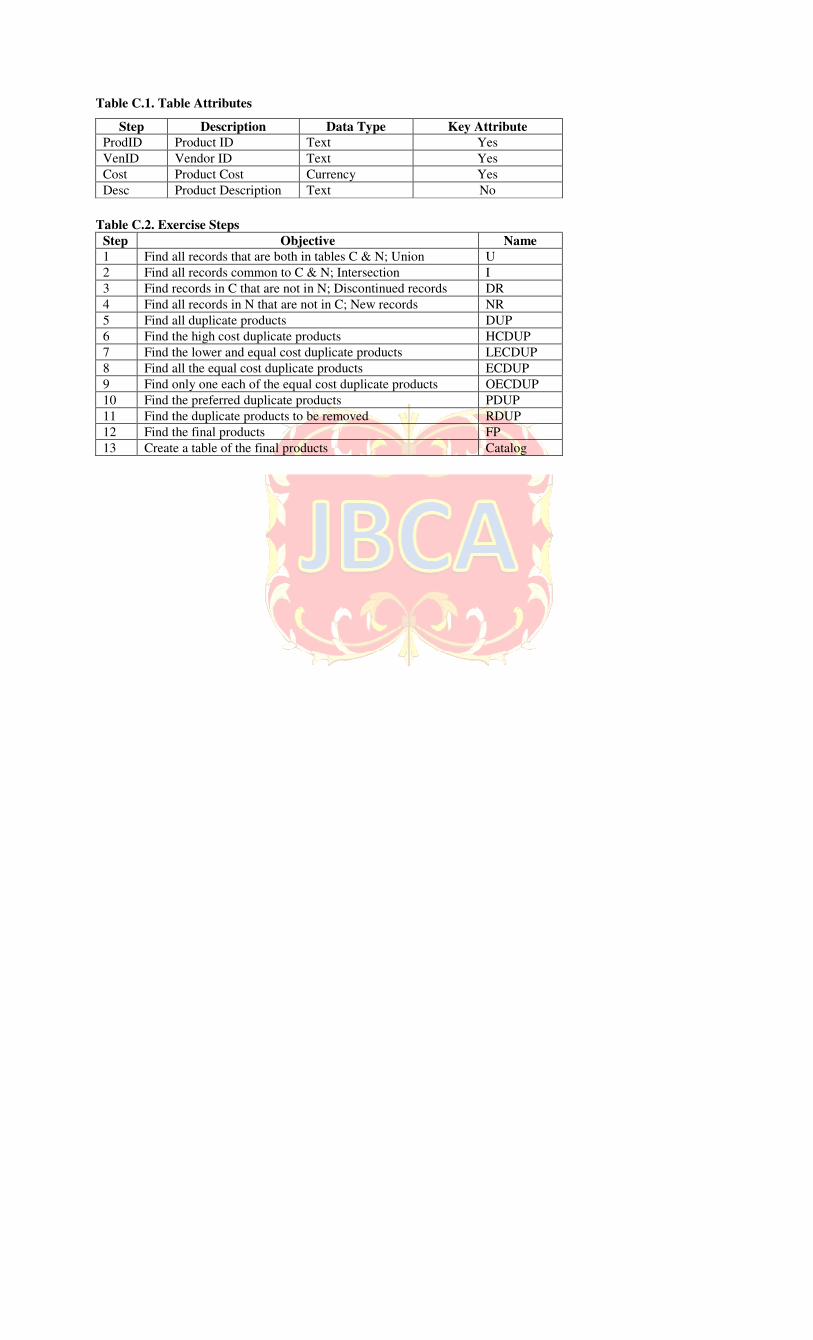
Table C.1. Table Attributes

Step Description Data Type Key Attribute

ProdID Product ID Text Yes

VenID Vendor ID Text Yes

Cost Product Cost Currency Yes

Desc Product Description Text No

Table C.2. Exercise Steps

Step Objective Name

1 Find all records that are both in tables C & N; Union U

2 Find all records common to C & N; Intersection I

3 Find records in C that are not in N; Discontinued records DR

4 Find all records in N that are not in C; New records NR

5 Find all duplicate products DUP

6 Find the high cost duplicate products HCDUP

7 Find the lower and equal cost duplicate products LECDUP

8 Find all the equal cost duplicate products ECDUP

9 Find only one each of the equal cost duplicate products OECDUP

10 Find the preferred duplicate products PDUP

11 Find the duplicate products to be removed RDUP

12 Find the final products FP

13 Create a table of the final products Catalog

Mapping Relation Algebra Operators

Figure C.1. Products Database Tables C and N

ProdID VenID Cost Desc ProdID VenID Cost Desc

NWTB-34 D $10.50 Beer NWTB-1 D $13.50 Chai

NWTB-43 B $34.50 Coffee NWTB-34 D $10.50 Beer

NWTB-81 C $2.00 Green Tea NWTB-43 B $36.50 Coffee

NWTB-87 G $2.00 Tea NWTB-43 C $37.00 Coffee

NWTBGM-21 A $7.50 Scones NWTB-43 D $36.00 Coffee

NWTBGM-85 A $9.00 Brownie Mix NWTB-81 C $2.00 Green Tea

NWTBGM-86 A $10.50 Cake Mix NWTB-87 G $2.00 Tea

NWTC-82 A $2.00 Granola NWTBGM-19 A $6.90 Biscuit Mix

NWTC-82 A $3.00 Hot Cereal NWTBGM-21 A $7.50 Scones

NWTCA-48 J $9.56 Chocolate NWTBGM-85 A $9.00 Brownie Mix

NWTCFV-17 F $29.25 Fruit Cocktail NWTBGM-86 A $10.50 Cake Mix

NWTCFV-88 F $1.00 Pears NWTC-82 A $2.00 Granola

NWTCFV-89 F $1.00 Peaches NWTC-82 A $3.00 Hot Cereal

NWTCFV-90 F $1.00 Pineapple NWTCA-48 J $9.56 Chocolate

NWTCFV-91 F $1.00 Cherry Pie Filling NWTCFV-88 F $1.00 Pears

NWTCFV-92 F $1.00 Green Beans NWTCFV-89 F $1.00 Peaches

NWTCFV-93 F $1.00 Corn NWTCFV-90 F $1.00 Pineapple

NWTCFV-94 F $1.00 Peas NWTCFV-91 F $1.00 Cherry Pie Filling

NWTCO-3 J $7.50 Syrup NWTCFV-92 F $1.00 Green Beans

NWTCO-4 J $16.50 Cajun Seasoning NWTCFV-93 F $1.00 Corn

NWTCO-77 J $9.75 Mustard NWTCFV-94 F $1.00 Peas

NWTCS-83 I $0.50 Potato Chips NWTCM-40 G $13.80 Crab Meat

NWTD-72 E $26.10 Mozzarella NWTCM-95 G $0.50 Tuna Fish

NWTDFN-14 B $17.44 Walnuts NWTCM-96 G $2.00 Smoked Salmon

NWTDFN-51 B $39.75 Dried Apples NWTCO-3 J $7.50 Syrup

NWTDFN-7 B $22.50 Dried Pears NWTCO-4 J $16.50 Cajun Seasoning

NWTDFN-74 F $8.50 Almonds NWTCO-77 J $9.75 Mustard

NWTDFN-80 B $3.00 Dried Plums NWTCS-83 I $0.50 Potato Chips

NWTG-52 A $5.25 Long Grain Rice NWTD-72 E $26.10 Mozzarella

NWTJP-6 D $18.00 Boysenberry Spread NWTDFN-14 B $17.44 Walnuts

NWTJP-6 B $60.75 Marmalade NWTDFN-14 F $16.50 Walnuts

NWTJP-6 D $60.75 Marmalade NWTDFN-51 B $39.75 Dried Apples

NWTO-5 J $16.01 Olive Oil NWTDFN-7 B $22.50 Dried Pears

NWTP-56 A $28.50 Gnocchi NWTDFN-74 B $7.50 Almonds

NWTP-57 A $14.63 Ravioli NWTDFN-74 C $7.50 Almonds

NWTS-65 H $15.79 Hot Pepper Sauce NWTDFN-74 F $8.50 Almonds

NWTS-66 H $12.75 Tomato Sauce NWTDFN-80 B $3.00 Dried Plums

NWTS-8 H $30.00 Curry Sauce NWTG-52 A $5.25 Long Grain Rice

NWTSO-41 F $7.24 Clam Chowder NWTJP-6 B $18.75 Boysenberry Spread

NWTSO-98 F $1.00 Vegetable Soup NWTJP-6 D $18.00 Boysenberry Spread

NWTSO-99 F $1.00 Chicken Soup NWTJP-6 F $17.50 Boysenberry Spread

NWTJP-6 B $60.75 Marmalade

NWTJP-6 D $60.75 Marmalade

NWTO-5 J $16.01 Olive Oil

NWTP-56 A $28.50 Gnocchi

NWTP-57 A $14.63 Ravioli

NWTSO-41 F $7.24 Clam Chowder

NWTSO-98 F $1.00 Vegetable Soup

NWTSO-99 F $1.00 Chicken Soup

Table C Table N

Mapping relation algebra operators into SQL queries: A … · · 2015-07-17Mapping relation...

Documents

Transcript of Mapping relation algebra operators into SQL queries: A … · · 2015-07-17Mapping relation...