92

Chapter 6

Mapping photonic entanglement intoand out of quantum memories

This chapter is largely based on ref. 30. Reference30 refers to the then current literature in 2008 at the time of

publication.

6.1 Introduction

In the quest to achieve quantum networks over long distances1,227, an area of considerable activity has been

the interaction of light with atomic ensembles comprised of a large collection of identical atoms (ref. 4, see

also chapter 1). In the regime of continuous variables, a particularly notable advance has been the tele-

portation of quantum states between light and matter60. For discrete variables with photons taken one by

one, important achievements include the efficient mapping of collective atomic excitations to single photons

(refs. 76,77,79,80, chapter 2), the realization of entanglement between distant ensembles (refs. 27,34, chapter 3)

and, recently, entanglement distribution involving two pairs of ensembles (ref. 36, chapter 4). The first step

toward entanglement swapping has been made (ref. 37, chapter 5), and light-matter teleportation has been

demonstrated with post-diction112.

In all these cases, progress with single photons has relied upon probabilistic schemes following the

measurement-induced approach developed in the seminal paper by Duan, Lukin, Cirac and Zoller (DLCZ)4

and subsequent extensions49. For the DLCZ protocol, heralded entanglement is generated by detecting a

single photon emitted indistinguishably by one of two ensembles. Intrinsically, the probability p to prepare

entanglement with only 1 excitation shared between two ensembles is related to the quality of entanglement,

since the likelihood for contamination of the entangled state by processes involving 2 excitations likewise

scales as p (ref. 34, chapter 3), and results in low success probability. Although the degree of stored entan-

glement can approach unity for the (rare) successful trials (ref. 34, chapter 3), the condition p 1 dictates

reductions in the count rate and compromises in the quality of the resulting entangled state (e.g., as p → 0,

processes such as stray light scattering and detector dark counts become increasingly important). Further-

93

more, for finite memory time, subsequent connection of entanglement becomes increasingly challenging

(ref. 37, chapter 5).

The separation of processes for the generation of entanglement and for its storage enables this draw-

back to be overcome. In this chapter, we demonstrate such a division by way of reversible mapping of an

entangled state into a quantum memory. The mapping is obtained by using adiabatic passage based upon

dynamic electromagnetically induced transparency (EIT) (refs. 86,88,89,94, see also sections 2.5 and 6.9 for de-

tails). Storage and retrieval of optical pulses have been demonstrated previously, for both classical pulses90,91

and single-photon pulses92,93. Adiabatic transfer of a collective excitation has been demonstrated between

two ensembles coupled by a cavity mode29, which can provide a suitable approach for generating on-demand

entanglement over short distances. However, for efficient distribution of entanglement over quantum net-

works, reversible mapping of an entangled state between matter and light, as illustrated in Fig. 6.1a, has not

been addressed until now.

In our experiment, entanglement between two atomic ensembles La, Ra is created by first splitting a sin-

gle photon into two modes Lin, Rin to generate an entangled state of light228–230. This entangled field state is

then coherently mapped to an entangled matter state for La, Ra. On demand, the stored atomic entanglement

for La, Ra is converted back into entangled photonic modes Lout, Rout. As opposed to the original DLCZ

scheme, our approach is inherently deterministic, suffering principally from the finite efficiency of mapping

single excitations to and from an atomic memory, with efficiency 50 % having been achieved. Moreover,

the contamination of entanglement for La, Ra from processes involving 2 excitations can be arbitrarily sup-

pressed (independent of the mapping probabilities) with continuing advances in on-demand single-photon

sources231. Our experiment thereby provides a promising avenue to distribute and store quantum entangle-

ment deterministically over remote atomic ensembles for scalable quantum networks232 (see also chapter 10

for a potential application of this scheme for hybrid quantum networks).

6.2 Deterministic quantum interface between matter and light

The experimental setup is depicted in Fig. 6.1. Our single-photon source is based on Raman transitions in

an optically thick cesium ensemble4,76, called a source ensemble (see section 6.8). This system generates

28-ns-long single photons (resonant with 6S1/2, F = 4 ↔ 6P3/2, F = 4 transition) in a heralded fashion76.

The single photons are polarized at 45 from the eigen-polarizations of the beam displacer BD1 (Fig. 1b)

which splits them into entangled optical modes Lin, Rin (called the signal modes) to produce, in the ideal

case, the following state1√2(|0Lin|1Rin+ eiφin |1Lin|0Rin). (6.1)

The next stage consists of coherently mapping the photonic entanglement for Lin, Rin into atomic ensem-

bles La, Ra (called the memory ensembles) within a single cloud of cold cesium atoms in a magneto-optical

94

gs

e

gs

e

Figure 6.1: Overview of the experiment. a, Reversible mapping. Illustration of the mapping of an entan-gled state of light into and out of a quantum memory (QM) with controllable storage time τ . b, Photonic“entangler.” A beam displacer BD1 splits an input single photon into two orthogonally polarized, entangledmodes Lin, Rin, which are spatially separated by 1 mm. With waveplates λ/2 and λ/4, the signal fieldssignal for Lin, Rin and control fields Ω(L,R)

c (t) are transformed to circular polarizations with the same helicityalong each path L,R, and copropagate with an angle of 3. c, Quantum interface for reversible mapping.Photonic entanglement between Lin, Rin is coherently mapped into the memory ensembles La, Ra by switch-ing Ω(L,R)

c (t) off adiabatically. After a programmable storage time, the atomic entanglement is reversiblymapped back into optical modes Lout, Rout by switching Ω(L,R)

c (t) on. Relevant energy diagrams for thestorage and retrieval processes are shown in the insets. States |g, |s are the hyperfine ground states F = 4,F = 3 of 6S1/2 in atomic cesium; state |e is the hyperfine level F = 4 of the electronic excited state 6P3/2.d, Entanglement verification. After a λ/4 plate, the beam displacer BD2 combines modes Lout, Rout into onebeam with orthogonal polarizations. With (λ/2)v at θc = 22.5 before the polarization beamsplitter (PBSD),single photon interference is recorded at detectors D1, D2 by varying the relative phase φrel by a Berek com-pensator. With (λ/2)v at θ0 = 0, photon statistics for each mode Lout, Rout are measured independently.

trap (MOT) (Fig. 6.1c). Ensembles La, Ra are defined by the well-separated optical paths of the entangled

photonic modes Lin, Rin (section 6.6). To avoid dissipative absorption for the fields in modes Lin, Rin for

our choice of polarization93, we spin-polarize the atomic ensemble into a clock state |F = 4,mF = 0(section 6.6). Initially, the strong control fields Ω(L,R)

c (resonant with 6S1/2, F = 3 ↔ 6P3/2, F = 4

transition) open transparency windows Ω(L,R)c (0) in La, Ra for the signal modes. As the wavepacket of the

signal field propagates through each ensemble, the control fields Ω(L,R)c (t) are turned off in 20 ns by an

electro-optical intensity modulator, thereby coherently transforming the fields of the respective signal modes

to collective atomic excitations within La, Ra. This mapping leads to an entanglement between quantum

memories La, Ra, with atomic state 1√2(|g

La|sRa+ eiφa |sLa|gRa

). After a user-defined delay, chosen here

to be 1.1 µs, the atomic entanglement is converted back into entangled photonic modes by switching on the

control fields Ω(L,R)c (t) (section 6.9), with a photon state 1√

2(|0Lout|1Rout + eiφout |1Lout|0Rout). The con-

95

Figure 6.2: Single-photon storage and retrieval for a single ensemble. a, Input. The data points are themeasured probability pc for the signal field, a single photon generated from a separate “offline” source atomicensemble76. The red solid line represents a Gaussian fit of 1/e width of 28 ns. b, Storage and retrieval. Thepoints around τ = 0 µs represent “leakage” of the signal field due to the finite optical depth and length ofthe ensemble. The points beyond τ = 1 µs show the retrieved signal field. The overall storage and retrievalefficiency is 17 ± 1 %. The blue solid line is the estimated Rabi frequency Ωc(t) of the control pulse. Thered solid curve is from a numerical calculation solving the equation of motion of the signal field in a dressedmedium (ref. 86, chapter 2). Error bars give the statistical error for each point.

trolled readout allows the extensions to quantum controls for entanglement connection and distribution by

way of asynchronous preparation (refs. 36,37, chapters 4 and 5).

6.2.1 Single-photon storage and retrieval

For a given optical depth d0, there is an optimal Rabi frequency Ωc(t) for the control field. In our experiment,

d0 and Ωc(0) are 15 and 24 MHz, respectively. An example of our measurements of the EIT process for a

single ensemble is presented in Fig. 6.2, which shows the input single-photon pulse (Fig. 6.2a) and its storage

and retrieval (Fig. 6.2b); see also chapter 2. Due to finite d0, small length (≈ 3 mm) of the ensemble and the

turn-off time of the intensity modulator, there is considerable loss in the storage process, as evidenced by the

counts around τ = 0 µs in Fig. 6.2b. The peak beyond τ = 1 µs represents the retrieved pulse after 1.1 µs of

storage. Overall, we find good agreement between our measurements and the numerical calculation following

the methods of ref. 86, using the fitted function of the input signal field (Fig. 6.2a) as the initial condition, with

all other parameters from independent measurements (section 6.9). We find the overall storage and retrieval

efficiency of ηsr = 17± 1 %, also in agreement with the simulation of ηtheorysr = 18 %.

6.2.2 Entanglement verification

With these results in hand for the individual La, Ra ensembles, we next turn to the question of verification

of entanglement for the optical modes of Lin, Rin and Lout, Rout. We follow the protocol introduced in ref. 27

96

by (1) reconstructing a reduced density matrix ρ constrained to a subspace containing no more than one ex-

citation in each mode, and (2) assuming that all off-diagonal elements between states with different numbers

of photons vanish, thereby obtaining a lower bound for any purported entanglement. In the photon-number

basis |nL,mR with n,m = 0, 1, the reduced density matrix ρ is written as (ref. 27, chapter 3)

ρ =1

P

p00 0 0 0

0 p10 d 0

0 d∗ p01 0

0 0 0 p11

. (6.2)

Here, pij is the probability to find i photons in mode Lk and j in mode Rk, d V (p10+p01)2 is the coherence

between |1L0Rk and |0L1Rk, P = p00 + p10 + p01 + p11, and V is the visibility for interference between

modes Lk, Rk, with k ∈ in, out. The degree of entanglement of ρ can be quantified in terms of concurrence,

C = 1P

max(0, 2|d| − 2√p00p11), which is a monotone function of entanglement, ranging from 0 for a

separable state to 1 for a maximally entangled state178.

6.3 Coherent and reversible quantum interface for photonic entangle-

ment

6.3.1 Quantum-state tomography on the input photonic state

We first perform tomography on the input modes Lin, Rin to verify that they are indeed entangled. To this end,

we remove the memory ensembles to transmit directly the signal fields into the verification stage, following

our protocol of complementary measurements as described in Fig. 6.1d (See section 6.7). The interference

fringes between the two input modes are shown in Fig. 6.3a. From the independently determined propagation

and detection efficiencies, we use the measurements at D1, D2 to infer the quantum state for the input modes

Lin, Rin entering the faces of La, Ra, with the reconstructed density matrix ρin given in Fig. 6.3a. The

concurrence derived from ρin is Cin = 0.10 ± 0.02, so that the fields for Lin, Rin are indeed entangled.

The value of the concurrence is in good agreement with the independently derived expectation of C theoryin =

0.10 ± 0.01, which depends on the quality of the single photon and the vacuum component (i.e., the overall

efficiency) (ref. 34, chapter 3). Given a heralding click from our single-photon source, the probability to have

a single photon at the face of either memory ensemble is 15 %, leading to a vacuum component of 85 %. We

also independently characterize the suppression w of the two-photon component relative to a coherent state

(for which w = 1) and find w = 0.09±0.03. Our input entanglement is only limited by the current properties

of our single-photon source, which will be improved with the rapid advances in sources of single photons231.

97

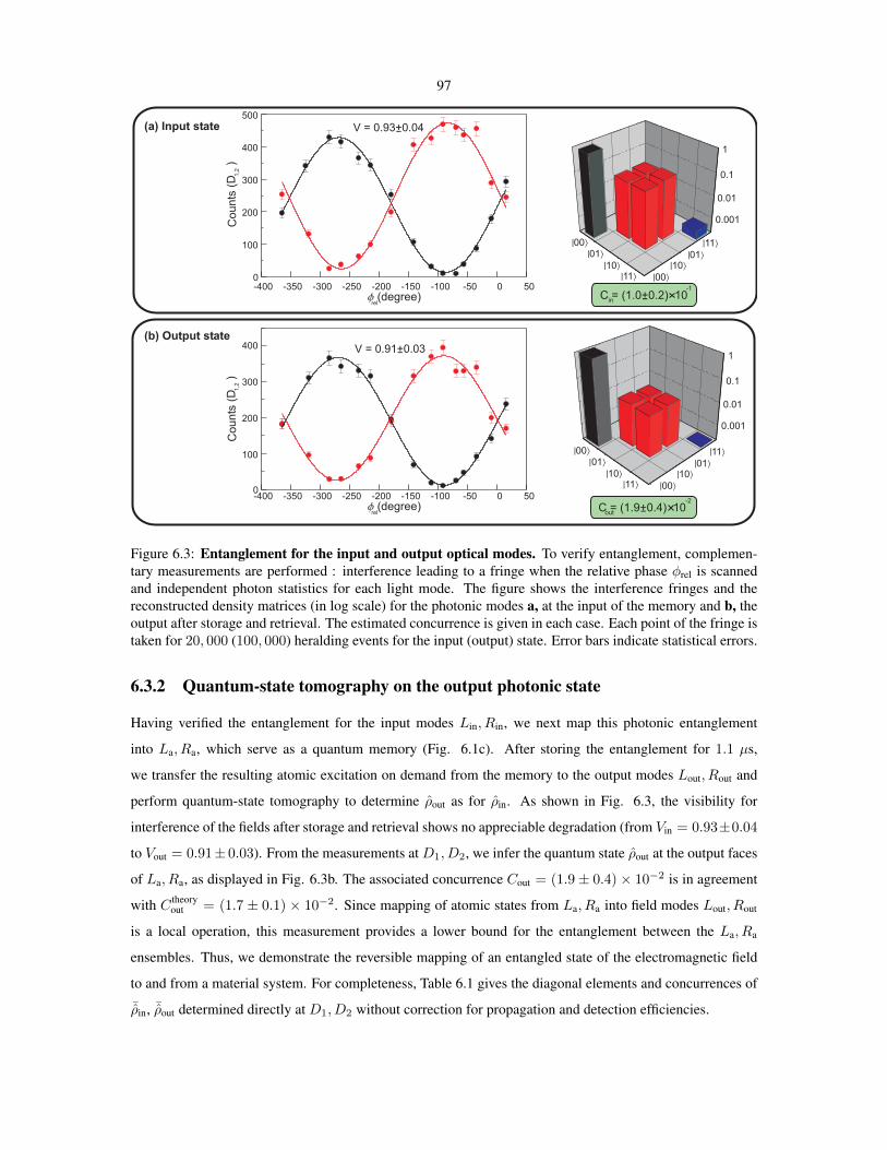
Figure 6.3: Entanglement for the input and output optical modes. To verify entanglement, complemen-tary measurements are performed : interference leading to a fringe when the relative phase φrel is scannedand independent photon statistics for each light mode. The figure shows the interference fringes and thereconstructed density matrices (in log scale) for the photonic modes a, at the input of the memory and b, theoutput after storage and retrieval. The estimated concurrence is given in each case. Each point of the fringe istaken for 20, 000 (100, 000) heralding events for the input (output) state. Error bars indicate statistical errors.

6.3.2 Quantum-state tomography on the output photonic state

Having verified the entanglement for the input modes Lin, Rin, we next map this photonic entanglement

into La, Ra, which serve as a quantum memory (Fig. 6.1c). After storing the entanglement for 1.1 µs,

we transfer the resulting atomic excitation on demand from the memory to the output modes Lout, Rout and

perform quantum-state tomography to determine ρout as for ρin. As shown in Fig. 6.3, the visibility for

interference of the fields after storage and retrieval shows no appreciable degradation (from Vin = 0.93±0.04

to Vout = 0.91± 0.03). From the measurements at D1, D2, we infer the quantum state ρout at the output faces

of La, Ra, as displayed in Fig. 6.3b. The associated concurrence Cout = (1.9± 0.4)× 10−2 is in agreement

with C theoryout = (1.7 ± 0.1) × 10−2. Since mapping of atomic states from La, Ra into field modes Lout, Rout

is a local operation, this measurement provides a lower bound for the entanglement between the La, Ra

ensembles. Thus, we demonstrate the reversible mapping of an entangled state of the electromagnetic field

to and from a material system. For completeness, Table 6.1 gives the diagonal elements and concurrences of¯ρin, ¯ρout determined directly at D1, D2 without correction for propagation and detection efficiencies.

98

6.4 Discussion and analysis

We emphasize that although the entanglement associated with ρout is heralded (because of the nature of our

single-photon source), our protocol for generation and storage of entanglement is intrinsically deterministic.

The transfer efficiency of entanglement from input modes to output modes of the quantum memory is limited

by the storage and retrieval efficiency ηsr of the EIT process. This transfer can be quantified by the ratio λ

of the concurrence Cout for the output state ρout to Cin for the input state ρin. For an ideal source of single

photons on-demand (with no vacuum component), the input concurrence is approximated by Cin αV ,

where α denotes the transmission efficiency of the single photon from the source to the entangler in Fig.

6.1b (ref. 34, chapter 3). Similarly, for the output, Cout αηsrV , where we assume that the visibility V is

preserved by the mapping processes. Thus, λ = CoutCin

ηsr, which therefore estimates the maximum amount

of entanglement in modes Lout, Rout for the case of an (ideal) single photon generated deterministically. In

our experiment, the entanglement transfer reaches λ = (20 ± 5) %. By way of optimal pulse shaping and

improved optical depth, the entanglement transfer can be greatly improved (section 6.10.2).

The performance of our quantum interface depends also on the memory time τm over which one can

faithfully retrieve a stored quantum state. For our system, independent measurements of ηr made by varying

the storage duration τ allow us to determine τm = 8 ± 1 µs, as limited by inhomogeneous Zeeman broad-

ening and motional dephasing (section 6.6 and chapter 2). Active and passive compensations of the residual

magnetic field would improve τm, along with improved optical trapping techniques (chapter 2).

6.5 Conclusion

In conclusion, our work provides the first realization of mapping an entangled state into and out of a quantum

memory. Our protocol alleviates the significant drawback of probabilistic protocols4, where low preparation

probabilities prevent its potential scalability37, and thus our strategy leads to efficient scaling for high-fidelity

quantum communication232. Our current results are limited by the large vacuum component of our avail-

able single-photon source, which principally reduces the degree of entanglement in the input, and by the

limited retrieval efficiency of the EIT process, which bounds the entanglement transfer to λ = (20 ± 5)

%. With improved retrieval efficiency and memory time, along with the rapid development of on-demand

Table 6.1: Experimentally determined diagonal elements and concurrences. We directly measure thediagonal elements pij and concurrences Cin, Cout for the density matrices ¯ρin, ¯ρout derived directly from de-tectors D1, D2 without correction for losses and detection efficiencies. Statistical errors are also given.

¯ρin ¯ρoutp00 0.9800± 0.0001 0.99625± 0.00003p10 (1.043± 0.008)× 10−2 (2.09± 0.02)× 10−3

p01 (0.957± 0.008)× 10−2 (1.67± 0.02)× 10−3

p11 (8± 2)× 10−6 (2± 2)× 10−7

C (1.28± 0.09)× 10−2 (2.5± 0.5)× 10−3

99

single-photon sources231, our protocol enables the deterministic generation, storage, and distribution of en-

tanglement among remote quantum memories for scalable quantum networks. Such networks have diverse

applications in quantum information science, including for quantum metrology, where quantum sensing is

provided by the atomic entanglement and readout by coherent mapping to the photonic modes (chapter 9).

In the broader context of quantum information theory, our experiment provides an important contribution

to the lively debate about “single-particle” entanglement228,229,233. One resolution of these discussions is

a gedanken experiment in which an entangled state for a single-particle is mapped into a two-particle sys-

tem by local operations, thereby verifying the presence of entanglement for the original “single-particle”

state233. Our experiment demonstrates that an entangled state with one photonic excitation shared between

two optical modes (see Eq. 6.1) can be converted into an entangled state for two atomic ensembles by way of

coherent mapping. The presence of entanglement between the two atomic ensembles is explicitly quantified

by the lower bound Cout = (1.9± 0.4)× 10−2, thereby realizing the proposal of ref. 233 for “single-particle”

entanglement.

6.6 Experimental details

A 22 ms preparation stage and 3 ms experiment run are conducted every 25 ms period. During the preparation

stage, atomic ensembles are loaded in a MOT for 18 ms and further cooled by optical molasses for 3 ms

where the MOT magnetic field is turned off. For 800 µs, we optically pump the atomic ensembles to the

6S1/2 |F = 4,mF = 0 state in atomic cesium. During this stage, the trapping beam is turned off while the

intensity of the repumping beam is reduced to 0.1Isat where Isat is the saturation intensity. The quantization

axis is chosen along the k-vector of the signal modes and defined by a pulsed magnetic field of 0.2 G.

A pair of counter-propagating Zeeman pumping beams (10 MHz red-detuned from 4 ↔ 4 transition and

linearly polarized along the quantization axis) illuminate the ensembles in a direction perpendicular to modes

Lin, Rin. The MOT repumping beam serves as a hyperfine pumping beam. The experiment is conducted

at a repetition rate of 1.7 MHz during a 3 ms interval before the next MOT loading cycle. A small bias

field of 10 mG is left on to define the quantization axis for the experiment. The various photon statistics

throughout the experiment are detected by single-photon Si-avalanche Photodetectors (Perkin-Elmer SPCM-

AQR-13) where the pulse signals are stamped with 2 ns resolution into a file by a 4-channel event time

digitizer (FAST ComTec P7888) for data-acquisition. The overall transmission efficiencies (including the

detector and propagation efficiencies) are 12± 2 % and 14± 2 % for the ensembles La, Ra.

The limitations to our experiment imposed by inhomogeneous Zeeman broadening are described in ref. 34

(chapters 2–3). Possible misalignment between the quantization axis and the bias magnetic field is estimated

to be below 5 degrees. Following ref. 195, we are investigating active compensation of the residual magnetic

field to improve τm. In our experiment, the memory time τm was also plagued by the residual control laser

during storage due to finite extinction ratio 50 dB of the modulator (waveguide electro-optical modulator and

100

two sets of acousto-optical modulators), which set τm 1 ms. In addition, thermal motion of the atoms (at

Td = 150 µK) sets the memory time of τm 15 µs due to the motional dephasing, where optical trapping

may dramatically improve the coherence time for the collective excitations (chapter 2).

6.7 Operational verification of entanglement

Operationally, the various elements of ρ are obtained by recombining the Lk, Rk fields with a second beam

displacer, BD2, as illustrated in Fig. 6.1d, to obtain a single spatial mode with orthogonal polarizations for the

Lk, Rk fields (refs. 34,36, chapters 3 and 4), with k ∈ in,out. The diagonal elements of ρ are measured with

(λ/2)v set at 0 so that detection events at D1, D2 are recorded directly for the Lk, Rk fields. To determine

the off-diagonal components of ρ, the modes Lk, Rk are brought into interference with (λ/2)v set at 22.5,

as shown in Fig. 6.1d. By varying the relative phase φrel between the modes, we determine the visibility for

single-photon interference and thereby deduce d.

6.8 Single-photon generation

The single-photon source is based upon the protocol4,76 composed of time-delayed photon pairs, called fields

1,2 emitted from a cesium ensemble in a MOT called the source ensemble. The source ensemble is located

3 m from the memory ensembles, both of which are synchronized by a 80 MHz clock signal. For photon-

pair production, a sequence of write and read pulses illuminates the source ensemble. The single photon

generation is heralded by probabilistic detection of a Raman scattered field 1 from a write pulse (10 MHz

red-detuned from 4 ↔ 4 transition). Conditioned on the heralding signal, a strong read pulse (resonant to

3 ↔ 4 transition) maps the excitation into a photonic mode, field 2, with probability of 50 %, which then

propagates to the setup described in Fig. 6.1. The resulting conditional probability to have a single photon,

field 2, at the face of memory ensemble is 15 %. The separation between the entangled optical modes Lin, Rin

after the entangler is 1 mm and each of the modes is focused down to a 1/e full width of 50 µm at La, Ra.

The heralding signal triggers a control logic which disables the single-photon source and all associated laser

beams for the programmable duration of the storage process for the quantum interface (ref. 36, chapter 4). As

the retrieval process is in the slow-light regime, the temporal shape of the single photon is controlled by the

intensity of the read laser, thereby changing the group velocity of the field 2 in the source ensemble75,234.

6.9 EIT storage and retrieval

The coherent interface between the signal modes and collective spin waves is achieved by dynamically con-

trolling the EIT window Ωc(t), defined by the atom-light interaction of a resonant control field. A quantum

field propagating through an externally controlled dressed state medium is best described as a slow-light,

101

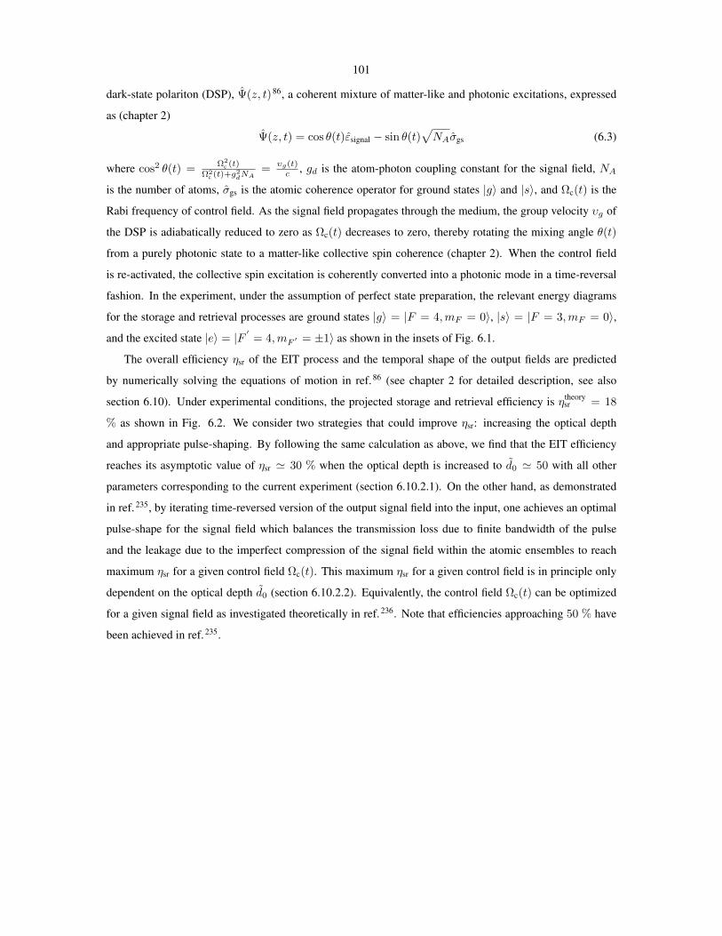
dark-state polariton (DSP), Ψ(z, t)86, a coherent mixture of matter-like and photonic excitations, expressed

as (chapter 2)

Ψ(z, t) = cos θ(t)εsignal − sin θ(t)NAσgs (6.3)

where cos2 θ(t) = Ω2c (t)

Ω2c (t)+g

2dNA

= υg(t)c

, gd is the atom-photon coupling constant for the signal field, NA

is the number of atoms, σgs is the atomic coherence operator for ground states |g and |s, and Ωc(t) is the

Rabi frequency of control field. As the signal field propagates through the medium, the group velocity υg of

the DSP is adiabatically reduced to zero as Ωc(t) decreases to zero, thereby rotating the mixing angle θ(t)

from a purely photonic state to a matter-like collective spin coherence (chapter 2). When the control field

is re-activated, the collective spin excitation is coherently converted into a photonic mode in a time-reversal

fashion. In the experiment, under the assumption of perfect state preparation, the relevant energy diagrams

for the storage and retrieval processes are ground states |g = |F = 4,mF = 0, |s = |F = 3,mF = 0,and the excited state |e = |F

= 4,mF

= ±1 as shown in the insets of Fig. 6.1.

The overall efficiency ηsr of the EIT process and the temporal shape of the output fields are predicted

by numerically solving the equations of motion in ref. 86 (see chapter 2 for detailed description, see also

section 6.10). Under experimental conditions, the projected storage and retrieval efficiency is ηtheorysr = 18

% as shown in Fig. 6.2. We consider two strategies that could improve ηsr: increasing the optical depth

and appropriate pulse-shaping. By following the same calculation as above, we find that the EIT efficiency

reaches its asymptotic value of ηsr 30 % when the optical depth is increased to d0 50 with all other

parameters corresponding to the current experiment (section 6.10.2.1). On the other hand, as demonstrated

in ref. 235, by iterating time-reversed version of the output signal field into the input, one achieves an optimal

pulse-shape for the signal field which balances the transmission loss due to finite bandwidth of the pulse

and the leakage due to the imperfect compression of the signal field within the atomic ensembles to reach

maximum ηsr for a given control field Ωc(t). This maximum ηsr for a given control field is in principle only

dependent on the optical depth d0 (section 6.10.2.2). Equivalently, the control field Ωc(t) can be optimized

for a given signal field as investigated theoretically in ref. 236. Note that efficiencies approaching 50 % have

been achieved in ref. 235.

102

6.10 Theoretical discussions

The dynamics of laser-induced coherence of atomic states can dramatically modify the optical response of

an atomic medium, leading to destructive quantum interferences between the excitation pathways95,96. In

this way, resonant absorption and refraction can be eliminated by way of electromagnetically induced trans-

parency (EIT)94. In this section, we describe a semi-classical theory of EIT. For a complete quantum theory

of dynamic EIT, I refer to chapter 2, whereby the equations of motions for the fields and atomic variables are

derived in a self-consistent manner. We also present our theoretical result of time-reversal optimization188

for ηsr using our experimental parameters30.

6.10.1 Static electromagnetically induced transparency

Here, we present a semi-classical theory for static EIT94,182,237,238. While the situation for dynamic EIT is

somewhat different, static EIT describes the phenomena of ultra-slow propagation of the signal field in a

coherent atomic medium88,239. We also examine the equivalence between the semi-classical model and the

full quantum model.

6.10.1.1 Semi-classical model of EIT

Electromagnetically induced transparency can be explained semi-classically in terms of (1) Fano-like quan-

tum interferences between the decay pathways of Autler-Townes resonances237,238, and (2) “adiabatic prepa-

ration” or “optical pumping” to a dark state in the dressed state picture86,179–181,183,184, as employed tradition-

ally in coherent population trapping (CPT) and stimulated Raman adiabatic passage (STIRAP), respectively.

In particular, I will adapt the latter approach (2), as the polaritonic quantum dynamics86 described in chapter

2 can be mapped to a semi-classical adiabatic passage in the setting of dark and bright states181.

As in chapter 2, we consider an effective (non-hermitian) Hamiltonian HEIT for an atomic ensemble

interacting with a weak classical signal field Es (Rabi frequency Ωs) and a strong control laser (Rabi frequency

Ωc) in the rotating frame (following the notations introduced in section 2.5), with

Heff = HEIT − iγgeσee − iγgsσss, (6.4)

where the system Hamiltonian HEIT for the EIT interaction is given by

HEIT/ = ∆cσee − δσss − (Ωsσeg + Ωcσes + h.c.) . (6.5)

∆c is the single-photon detuning for the control laser, and δ is the two-photon detuning between the signal

field and the control laser. Here, the decay channels (−iγgeσee, −iγgsσss) result in losses of atomic coher-

ences at rates γge and γgs. In the following discussions, I will assume a negligible ground-state dissipation

γgs 0 and resonant excitation by the control laser with ∆c = 0.

103

For open quantum systems, quantum-state evolution by a master equation in the Lindblad form (e.g., for

Eq. 6.5) is equivalent to that of a stochastic wave-function method (quantum-trajectory method) accompanied

by quantum jumpsa (refs. 164–166,240,241). Assuming a wave-function of the form |ψ(t) = cg(t)|g+cs(t)|s+ce(t)|e, the non-hermitian effective Hamiltonian Heff (Eq. 6.4) yields the following equations of motions

(from the Schrodinger’s equation),

cg = iΩ∗sce (6.6)

cs = −(γgs − iδ)cs + iΩ∗cce (6.7)

ce = −(γge − iδ)ce + iΩscg + iΩccs. (6.8)

Since Ωs Ωc and the initial state is |ψ(0) = |g, we assume that the probability amplitude remains

in cg(t) 1 for all time t. Fourier transforming Eqs. 6.7–6.8 (with ∂t → iw) and solving for cs, ce, we

obtain

cs(w) =ΩsΩ∗

c

(w − iγge − δ)(w − δ)− |Ωc|2

ce(w) =Ωs(w − δ)

(w − iγge − δ)(w − δ)− |Ωc|2.

The off-diagonal atomic polarization ρeg can thus be expressed as ρeg = c∗gce ce, while the normalized

linear susceptibility function is χs= ρeg

Ωs(see chapter 2). Redefining (δ−w) → ν, we arrive at the expression

for the normalized linear susceptibility χs

in Eq. 2.79 with

χs=

ν

|Ωc|2 − ν2 − iγgeν. (6.9)

The relationship between χs

and group velocity vg (and transparency window) is explained in chapter

2 for an ideal Λ-level system. In section 6.10.1.3, we further illustrate the importance of optical pumping

and polarization orientations of the control laser and the signal field for observing EIT in a Λ-level system

comprised of multiple Zeeman sublevels.

6.10.1.2 The emergence of dark and bright states

The underlying principle for the cancellation of absorption in EIT is directly related to the phenomena of

dark-state and coherent population trapping183. Let us examine the effective Hamiltonian Heff with δ = 0. In

aWe note that the effective Hamiltonian Heff (Eq. 6.4) does not capture the repopulations of σgg and σss due to spontaneousemissions (−iγgeσee). As a semi-classical analysis, we neglect the quantum jump processes 164,165 and only consider the evolution ofthe stochastic wave-function |ψ(t) under the effective Hamiltonian over time t. This approximation is valid in the quantum trajectorymethod for our initial condition cgg + css 1, as long as the jump probability is pjump = ψ| exp

i t0 dt(Heff − H

†eff)

|ψ

t0 dt

γge|cee|2 + γgs|css|2

1 for γgs 0.

104

=

Figure 6.4: Qualitative equivalence between electromagnetically induced transparency and coherentpopulation trapping. As shown by Eq. 6.10, the phenomena of EIT in the atomic bare-state basis can beequivalently described as a dark-state pumping process (CPT) in the dark- and bright-state basis for two-photon detuning δ = 0.

the dark- and bright-state picture, we may equivalently write Heff (Eq. 6.4) in the following way,

Heff/ = −iγgeσee − Ωeff (sin∗ θd|g+ cos∗ θd|s)

|b

e|− Ωeff|e (sin θdg|+ cos θds|) b|

, (6.10)

where θd = arctan(Ωs/Ωc) is the mixing angle, and Ωeff =

|Ωc|2 + |Ωs|2 is the effective Rabi frequency

which couples the bright state |b = sin∗ θd|g + cos∗ θd|s to the excited state |e. Similarly, we introduce

a sibling, a dark state |d = cos∗ θd|g − sin∗ θd|s (one of the three eigenstates of Heff) orthonormal to the

bright state |b, which does not couple to the excited state |e via Heff (thus, immune to spontaneous emission).

Here, I used the notations, sin∗ θd, cos∗ θd, to define the complex conjugates of sin θd, cos θd.

In the picture of dark- and bright-state basis (Eq. 6.10), the atomic level diagram in the bare-state picture

is transformed to a diagram akin to the case of optical pumping, as shown in Fig. 6.4. Here, the bright-state

|b couples dissipatively to the excited state |e with an effective Rabi frequency Ωeff, while the dark-state |dis decoupled from the signal field Es and the control laser Ωc. Thus, if the initial atomic state is prepared in

an admixture of both ground states (|g and |s), the coherently dressing Ωeff will “optically pump” the atoms

in the bright state |b to the dark state |d through the spontaneous emission from the excited state |e. As

there are little atoms left in |b after dark-state pumping (with negligible optical thickness for the |b ↔ |etransition), the atoms will be trapped in the dark state via coherent population trapping (CPT) and the signal

field will exhibit full spectroscopic transparency on resonance δ = 0.

In the case of EIT, the initial atomic state can further be prepared to the dark state |d |g (with

Ωs Ωc) prior to the EIT dressing (by means of optical pumping), from which excitations cannot occur.

Therefore, by rotating the mixing angle θd = 0 → π/4, we can adiabatically transfer the initial state to a

superposition state |d = 12 (|g − |s) of maximum atomic coherence σgs, as in stimulated Raman adiabatic

transfer181,184 (STIRAP). There is a qualitative similarity between the adiabatic following of |d and the

dynamics of the dark-state polariton Ψd. Heuristically considering the Fock state of the signal field, we can

105

write the dark state in a familiar form |d = cos∗ θd|ga, 1s− sin∗ θd|sa, 0s, identical to the single-excitation

dark-state |D, 1 = Ψ†d|ga, 0s (Eq. 2.69) in chapter 2. Hence, the quantum theory of dark-state polaritons86

(chapter 2) is associated with the classical picture of dark- and bright-states in CPT and STIRAP.

6.10.1.3 Importance of the Zeeman sublevels

In the presence of multiple Zeeman sublevels, the susceptibility function χs = 2g2dNA

wsχs

in Eq. 2.79 of

chapter 2 and Eq. 6.9 generalizes to a normalized form χs

of

χs(δ) =

1

Nc

mF

pmF |CFg,1,Fe

mF ,s,mF+s|2δ

|Ωc|2|CFs,1,FemF+s−c,c,mF+s

|2 − δ2 − iγgeδ, (6.11)

where Nc =

mFpmF |C

Fg,1,Fe

mF ,s,mF+s|2 is the normalization constant, s, c are the respective helicities

for the signal field and the control lasers, and Cf1,f2,f3m1,m2,m3

≡ f1m1f2m2|f3m3 are the Clebsch-Gordan coef-

ficients. In deriving Eq. 6.11, we assumed that the initial atomic state is ρa =

mFpmF |Fg,mF Fg,mF |.

For the ideal susceptibility function in Fig. 2.4 of chapter 2, the imaginary part of the susceptibility

is Im(χs) = 0 on resonance δ = 0, thereby providing a transparency window for the signal field. At

the same time, the real part of the linear susceptibility function Re(χs) provides a strong dispersion on

resonance for slow-light propagation. In the presence of Zeeman populations pmF , however, the coherent

atomic medium exhibits EIT only for specific polarization orientations s, c of the signal field and the

control lasers. Particularly, if the one of the Clebsch-Gordan coefficients CFg,1,Fs

mF+s−c,c,mF+svanishes, the

uncoupled Zeeman populations may have sufficient optical depths to cause dissipative absorption of the signal

field and the absence of transparency.

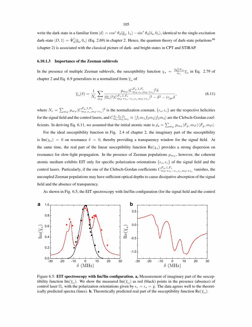
As shown in Fig. 6.5, the EIT spectroscopy with lin//lin configuration (for the signal field and the control

ba

-­30 -­20 -­10 0 10 20 30

-­1.0

-­0.5

0.0

0.5

-­30 -­20 -­10 0 10 20 300.0

0.2

0.4

0.6

0.8

1.0

Figure 6.5: EIT spectroscopy with lin//lin configuration. a, Measurement of imaginary part of the suscep-tibility function Im(χ

s). We show the measured Im(χ

s) as red (black) points in the presence (absence) of

control laser Ωc with the polarization orientations given by c = s = y. The data agrees well to the theoret-ically predicted spectra (lines). b, Theoretically predicted real part of the susceptibility function Re(χ

s).

106

ba

-­30 -­20 -­10 0 10 20 30-­1.0

-­0.5

0.0

0.5

1.0

-­30 -­20 -­10 0 10 20 300.0

0.2

0.4

0.6

0.8

1.0

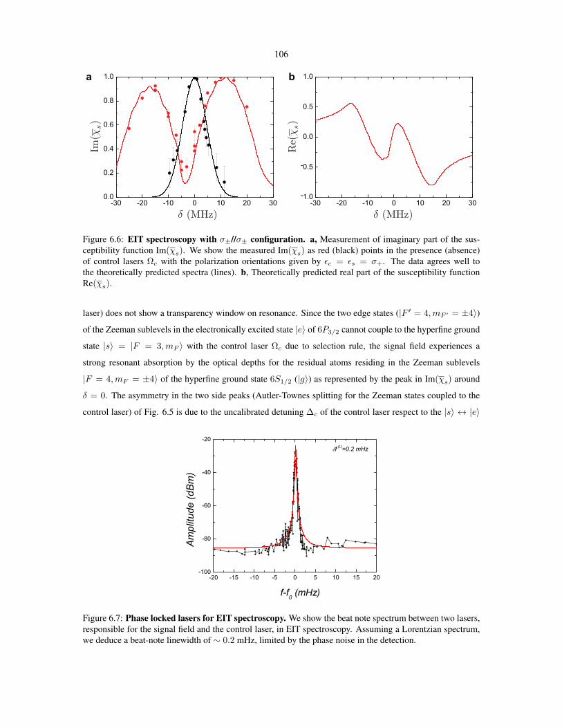
Figure 6.6: EIT spectroscopy with σ±//σ± configuration. a, Measurement of imaginary part of the sus-ceptibility function Im(χ

s). We show the measured Im(χ

s) as red (black) points in the presence (absence)

of control lasers Ωc with the polarization orientations given by c = s = σ+. The data agrees well tothe theoretically predicted spectra (lines). b, Theoretically predicted real part of the susceptibility functionRe(χ

s).

laser) does not show a transparency window on resonance. Since the two edge states (|F = 4,mF = ±4)of the Zeeman sublevels in the electronically excited state |e of 6P3/2 cannot couple to the hyperfine ground

state |s = |F = 3,mF with the control laser Ωc due to selection rule, the signal field experiences a

strong resonant absorption by the optical depths for the residual atoms residing in the Zeeman sublevels

|F = 4,mF = ±4 of the hyperfine ground state 6S1/2 (|g) as represented by the peak in Im(χs) around

δ = 0. The asymmetry in the two side peaks (Autler-Townes splitting for the Zeeman states coupled to the

control laser) of Fig. 6.5 is due to the uncalibrated detuning ∆c of the control laser respect to the |s ↔ |e

Amplitude (dBm)

Figure 6.7: Phase locked lasers for EIT spectroscopy. We show the beat note spectrum between two lasers,responsible for the signal field and the control laser, in EIT spectroscopy. Assuming a Lorentzian spectrum,we deduce a beat-note linewidth of ∼ 0.2 mHz, limited by the phase noise in the detection.

107

transition (which use as a fitting parameter in Fig. 6.5). The solid lines are the theoretical predictions based

on Eq. 6.11, with the assumption of the initial state pmF = 1/(2Fg + 1)

Instead, we now apply a signal field and a control laser with helicities s, c = σ± in Fig. 6.6. As

shown in Fig. 6.6a, the measured susceptibility function clearly demonstrates electromagnetically induced

transparency around δ = 0. Here, the red-detuned offset of the transparency window is due to the presence of

the detuning ∆c of the control laser. In Fig. 6.5b, we also show the real part of the linear susceptibility, similar

to the result obtained for the ideal Λ-level system (Fig. 2.4). Furthermore, in our experiment30 (Fig. 6.1),

we initialize the atoms to a clock state |g = |F = 4,mF = 0. With c,s = σ±, the coherent dressings by

the control and signal fields allow clock-state preserving transitions (section 6.6), which form a Λ-level with

|g = |F = 4,mF = 0, |s = |F = 4,mF = 0, and |e = |F = 4,mF = ±1. By optically pumping the

ensemble to |g = |F = 4,mF = 0 with efficiency ∼ 90 %, we achieve a maximum transparency T = 95

% on resonance.

6.10.2 Dynamic electromagnetically induced transparency

In chapter 2, we derived the Heisenberg-Langevin equations of motions in the polaritonic picture. In this sec-

tion, we numerically solve the equations of motions and compare the theoretically simulated spatio-temporal

modes Es to the experiment, where we store and retrieve a coherent state |α for various optical depths. We

also show a theoretical simulation of time-reversal optimization of the storage and retrieval efficiency ηsr

based on ref. 188 for our experimental parameters30.

6.10.2.1 Scaling behavior to optical depth and pitfalls via dissipative absorption

As we discussed in chapter 2, the dynamics of the signal field Es(z, t) and the collective atomic excitation

S(z, t) in the one-dimensional approximation is governed by the following coupled equations of motions

(Eqs. 2.85–2.87),

(∂t + c∂z) Es(z, t) = igdnA(z)L√NA

P(z, t) (6.12)

∂tP(z, t) = −(γge + i∆)P(z, t) + igd

NAEs(z, t) + iΩc(z, t)S +2γgeFP (6.13)

∂tS(z, t) = −γgsS(z, t) + iΩ∗c(z, t)P +

2γgsFS , (6.14)

where P(z, t) is the atomic polarization |g − |e induced by the quantum field Es(z, t) in the presence

of coherent dressing Ωc(z, t). Assuming a coherent-state input, we numerically solve the complex-value

equations of motions (Eqs. 6.12–6.14) by neglecting the Langevin terms FS = FP = 0, which do not

contribute to normally-ordered expectation values. Here, we fit the atomic ensemble with a Gaussian spatial

profile to infer the atomic density nA(z) = 2NA√πL

exp−4z2/L2

from the fluorescence measurement, and

108

the spatio-temporal mode of the control laser Ωc(t− z/c) approximated by

Ωc(x) = Ωc ×tanh [c1x] + tanh [−c2(x− τ)]

2, (6.15)

with the parameters Ωc, c1, c2 determined from independent measurements on the intensity of the control

laser. NA is determined from the measured value of the optical depth d0 for the |g − |e transition (optical

depth is defined as the transmission T = e−d0 of the signal field absent the control laser). For the details of

the derivations for Eqs. 6.12–6.14, I refer to the discussions in chapter 2.

Experimentally, we apply a control laser with Ωc 24 MHz (rise and fall times δtc = 1/c1 = 1/c2 7

ns, defined as the time-scales resulting in an intensity changes of 10%−90%) and a phase-locked signal laser

Es (Fig. 6.7) resonant to |g− |e transition (with two-photon detuning δ = 0) in a counter-intuitive order181.

The signal field Es is assumed to be in a coherent state |α with |α|2 0.3 per pulse (Gaussian pulse width

30 ns for the incoming signal pulse). The relative delay between Ωc and Es is tuned to maximize the storage

and retrieval efficiency ηsr. As in the main experiment30 (sections 6.1–6.9), we prepare the atomic ensemble

into the clock state |g = |F = 4,mF = 0 by optical pumping. We reduce the repetition rate of the laser

cooling and trapping cycle from 40 Hz to 0.2 Hz in order to increase the atomic density242,243 via compressed

MOT (CMOT)243 for 200 ms after the normal MOT loading and cooling (4 s). We then further cool the atoms

with polarization gradient cooling for 50 ms, followed by optical pumping (1 ms) to the clock state. With

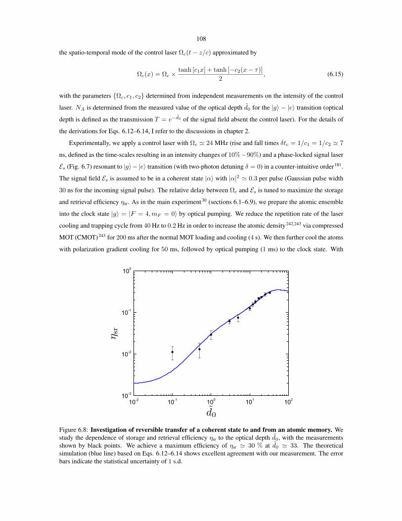
10-­2 10-­1 100 101 10210-­3

10-­2

10-­1

100

Figure 6.8: Investigation of reversible transfer of a coherent state to and from an atomic memory. Westudy the dependence of storage and retrieval efficiency ηsr to the optical depth d0, with the measurementsshown by black points. We achieve a maximum efficiency of ηsr 30 % at d0 33. The theoreticalsimulation (blue line) based on Eqs. 6.12–6.14 shows excellent agreement with our measurement. The errorbars indicate the statistical uncertainty of 1 s.d.

109

the improved setup, we achieve a maximum resonant optical depth of d0 50, albeit with reduced optical

pumping efficiency ∼ 70% due to radiation trapping, compared to the main experiment30 (sections 6.1–6.9).

The optical depth d0 is varied by tuning the value of the magnetic field to the desired value during the normal

MOT phase (before compression).

In Fig. 6.8, we show the overall transfer efficiency ηsr for storing and retrieving a coherent state |α in an

atomic ensemble (with storage time τ = 1 µs) as a function of optical depth d0 (see e.g., Fig. 2.6 for a time-

domain measurement at d0 = 20). In particular, we achieve a maximum storage and retrieval efficiency of

ηsr = 30± 2 % at optical depth d0 33. We also find excellent agreement between the theoretical predicted

EIT efficiency ηtheorysr (d0) and the experimentally measured ηsr. We emphasize that for higher optical depth

d0 60 (a region beyond the capability at the time), the storage and retrieval efficiency ηsr is expected to

decrease, due to the reduced bandwidth of the EIT medium at high d0 (chapter 2, see also Fig. 6.10). For

further improvement in ηsr, it is thus important to increase the intensity of the control laserb for higher d0.

In order to optimize ηsr for a finite d0, we need to compromise the control laser’s intensity between two

competing regimes. On the one hand, (1) a large Rabi frequency Ωc is preferred to increase bandwidth of

the EIT medium and to avoid dissipative absorption of Es. On the other hand, (2) a sufficiently small Ωc is

required to compress the signal field’s wavepacket inside the ensemble for avoiding significant leakage. In

analogy, these two competing effectsc at finite d0 can be cast in terms of the proper shaping of the spatio-

temporal mode of the signal field Es for a fixed Ωc. In the next section, we discuss an iterative optimization

strategy based on the works by Gorshkov et al.187–189, which leads to global maximization of ηsr in the fully

adiabatic regime, as demonstrated experimentally by Novikova et al.235.

6.10.2.2 Iterative optimization strategy based on time-reversal symmetry

In the fully adiabatic regime, the mapping process is well described by the dynamics of dark-state polariton

Ψd(z, t) = cos θd(t)Es(z, t) − sin θd(t)S(z, t) with a beamsplitter-like Hamiltonian H (map)int (Eq. 2.84) in

chapter 2, given by

H (map)int = iθd(z, t)

Es(z, t)S†(z, t)− E†

s(z, t)S(z, t)

. (6.16)

θd(z, t) gives the rate of change in the mixing angle θd(z, t), which we assume to be small in order for

adiabatic passage (chapter 2). The unitary transformation U (map)int (t) = exp(− i

Lt

0 dtL

0 dzH (map)int (z, t))

bWith a large Rabi frequency Ωc for the control laser, there may be a non-negligible contribution from a competing four-wavemixing process 244, where the atoms initially at |g is off-resonantly driven to |s by Ωc generating an anti-Stokes photon, followed bya resonant scattering back to |g with Ωc seeded by the signal field (Stokes photon). We do not consider this four-wave mixing processin our calculation, as it is suppressed by the large ground-state splitting ∼ 9 GHz.

cFor a given Ωc, we need to keep the signal pulse Es as short as possible to compress Es within the atomic sample and to avoidleakage. On the other hand, we need to broaden the spatial extent of Es as much as possible to reduce its pulse bandwidth well belowthe EIT bandwidth of the coherent atomic medium.

110

describes the mapping process, where we individually define the storage (ηs) and retrieval (ηr) efficiencies as

ηs =

dzS†(z, ts)S(z, ts)dzE†

s (z, t0)Es(z, t0)(6.17)

ηr =

dzE†

s(z, tf )Es(z, tf )

dzS†(z, tr)S(z, tr), (6.18)

evaluated at the respective times ts (falling edge) and tr (rising edge) with delay τ = tr − ts. Es(z, t0) and

Es(z, tf ) give the initial (incoming) and final (outgoing) states of the signal field.

Qualitatively, it is easier to understand the optimal retrieval strategy for ηr than to understand the optimal

storage ηs, as we assume a pre-existing collective spin-wave with a profile S†(z, tr)S(z, tr) at time tr.

In this case, unlike the storage, we are not restrained by the control laser due to the leakage of the signal

field. In practice, however, an abrupt activation of Ωc(z, t) can reduce the retrieval efficiency by the non-

adiabatic transition of Ψd(z, t) to the bright-state polariton Ψb(z, t). Here, we give a heuristic argument for

the optimal ηoptr (ref. 188), where we assume a fully adiabatic regime for Ωc(z, t) and an optimally shaped

S†(z, tr)S(z, tr). For a rigorous proof in the adiabatic regime, I refer to the original works in refs. 187–189.

We then show that the time-reversed version of the optimal retrieval process leads to an optimal storage with

efficiency ηopts = ηopt

r .

We first consider the forward retrieval in a Gaussian signal mode with beam-waist w0 (section 2.3.2.2).

Beyond the Rayleigh range, the solid-angle Ωsolid of this mode is given by Ωsolid λ2

4πw20 ln 2

. The collectively

enhanced scattering rate into this mode is then simply Γc = ΩsolidN2AΓ0 = λ

2

4πw20 ln 2

N2AΓ0, whereas the

scattering rate into all other modes is given approximately by Γn NAΓ0. Here, Γ0 = 2πγge is the single-

atom scattering rate. The optimal retrieval efficiency ηoptr is then given by

ηoptr =

Γc

Γc + Γn

3d0

3d0 + 8 1− 8

3d0, (6.19)

where we used the relations for resonant absorption cross-section σ0 = 3λ2/2π and optical depth d0 NAσ0/(πw2

0). Thus, we find that the optimal retrieval efficiency for ηoptr depends only on the optical depth

d0 = g2dNA

γgeκeff(where κeff = c/L), which plays the role of a cooperativity parameter (chapter 2).

From the qualitative argument given above for achieving the optimal ηoptr , we now discuss the principle of

time-reversal as an optimization tool for storage ηs. We consider the storage map U (map)int (t) on the initial state

|ga, 1s given by |D, 1 = Ψ†d|ga, 0s in the Schrodinger picture. The storage probability ηs is then given by

ηopts = |sa, 0s|U (map)

int (t)|ga, 1s|2. (6.20)

Using the unitarity relation for U (map)†int (t) = U (map)

int (−t), we find that the storage efficiency is identical to the

retrieval efficiency,

ηopts = |ga, 1s|U

(map)int (−t)|sa, 0s|2 = ηopt

r , (6.21)

111

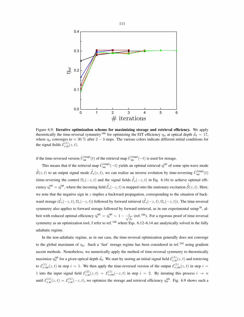
0 1 2 3 4 5 60.0

0.1

0.2

0.3

0.4

Figure 6.9: Iterative optimization scheme for maximizing storage and retrieval efficiency. We applytheoretically the time-reversal symmetry186 for optimizing the EIT efficiency ηsr at optical depth d0 = 17,where ηsr converges to 30 % after 2 − 3 steps. The various colors indicate different initial conditions forthe signal fields E(1)

s,in(z, t).

if the time-reversed version U (map)int (t) of the retrieval map U (map)

int (−t) is used for storage.

This means that if the retrieval map U (map)int (−t) yields an optimal retrieval ηopt

r of some spin-wave mode˜S(z, t) to an output signal mode ˜Es(z, t), we can realize an inverse evolution by time-reversing U (map)

int (t)

(time-reversing the control Ωc(−z, t) and the signal fields ˜Es(−z, t) in Eq. 6.16) to achieve optimal effi-

ciency ηopts = ηopt

r , where the incoming field ˜Es(−z, t) is mapped onto the stationary excitation ˜S(z, t). Here,

we note that the negative sign in z implies a backward propagation, corresponding to the situation of back-

ward storage ( ˜Es(−z, t),Ωc(−z, t)) followed by forward retrieval ( ˜Es(−z, t),Ωc(−z, t)). The time-reversal

symmetry also applies to forward storage followed by forward retrieval, as in our experimental setup30, al-

beit with reduced optimal efficiency ηoptr = ηopt

s ∼ 1 − 1√d0

(ref. 186). For a rigorous proof of time-reversal

symmetry as an optimization tool, I refer to ref. 188 where Eqs. 6.12–6.14 are analytically solved in the fully

adiabatic regime.

In the non-adiabatic regime, as in our case, the time-reversal optimization generally does not converge

to the global maximum of ηsr. Such a ‘fast’ storage regime has been considered in ref. 245 using gradient

ascent methods. Nonetheless, we numerically apply the method of time-reversal symmetry to theoretically

maximize ηoptsr for a given optical depth d0. We start by storing an initial signal field E(1)

s,in(z, t) and retrieving

to E(1)s,out(z, t) in step i = 1. We then apply the time-reversed version of the output E(1)

s,out(z, t) in step i =

1 into the input signal field E(2)s,in(z, t) = E(1)

s,out(−z, t) in step i = 2. By iterating this process i → n

until E(n)s,in(z, t) = E(n)

s,in(−z, t), we optimize the storage and retrieval efficiency ηoptsr . Fig. 6.9 shows such a

112

0 50 100 150 2000.00

0.15

0.30

0.45

0.60

0.75

d = 30

Adiabacity

0 1 2 3 4 50.00

0.25

0.50

0.75

1.00

# iterations

Figure 6.10: Time-reversal optimization of EIT transfer efficiency. We show the transfer efficiency ηsr asa function of optical depth d0. We also compare the result of the optimal ηopt

sr (red line) to ηsr (blue line) givenfor our experimental parameters in Fig. 6.8.

numerical process for optical depth d0 = 17 (with same parameters c1, c2,Ωc used in section 6.10.2.1)

starting from various initial conditions E(1)s,in(z, t), where we converge to the same maximum EIT efficiency

ηoptsr 30 % after 2− 3 iterations.

In addition, this numerical optimization scheme allows us to benchmark the maximum transfer efficiency

λ ηoptsr of entanglement as a function d0. In Fig. 6.10, we apply the time-reversal optimization as a function

of optical depth d0, shown as red line. We demonstrate that ηoptsr (red line) can be further improved relative

to the EIT efficiency ηsr of our experiment parameters (blue line) (see also Fig. 6.8) beyond d0 50. In

particular, unlike Fig. 6.8, we find a monotonic improvement in the transfer efficiency ηsr as a function of

optical depth d0. For reference, we indicate the boundary at which the adiabatic condition d0γgeδtc 1 is

met87.