Mapping Graphics Fundamentals for NT Course Guidehturner/ce127/micro.doc · Web viewMapping...
296
Mapping Graphics Fundamentals MICROSTATION LESSON MANUAL INSTRUCTOR DR. HOWARD TURNER P.L.S. 1 1
Transcript of Mapping Graphics Fundamentals for NT Course Guidehturner/ce127/micro.doc · Web viewMapping...
Mapping Graphics Fundamentals
MICROSTATION
LESSON MANUAL
INSTRUCTOR
DR. HOWARD TURNER P.L.S.
Mapping Sciences Center of ExcellenceCollege of Engineering
California State Polytechnic University, Pomona3801 W. Temple Ave.
Pomona CA 91768
1
1

Table of Contents
Lesson 1 - Windows Basics.................................................................................................................................................61.1 The Mouse................................................................................................................................................................61.2 Power On..................................................................................................................................................................61.3 Log On......................................................................................................................................................................61.4 Window Manipulations............................................................................................................................................71.4.1 Window Components and Sizing..........................................................................................................................71.4.2 Pull Down Menus..................................................................................................................................................91.4.3 Control Menu........................................................................................................................................................91.4.4 Scroll Bars...........................................................................................................................................................101.4.5 Switching Applications......................................................................................................................................10
Lesson 2 - The Windows Desktop.....................................................................................................................................112.1 The Desktop...........................................................................................................................................................112.2 Desktop Icons.........................................................................................................................................................112.3 Desktop Folders......................................................................................................................................................112.4 Arranging Desktop Icons.......................................................................................................................................122.5 Opening Groups using the Start button..................................................................................................................122.6 Arranging program Icons.......................................................................................................................................122.7 Copying Program Items.........................................................................................................................................122.8 Moving Program Items...........................................................................................................................................162.9 Additional Program Item Manipulations................................................................................................................162.10 Creating a Personal Desktop Folder.....................................................................................................................172.11 CVreating Items Within Folders..........................................................................................................................182.12 Modifying Program Properties.............................................................................................................................192.13 Security Dialog Box.............................................................................................................................................192.13.1 Logging Off.......................................................................................................................................................202.13.2 Shutting Down...................................................................................................................................................202.13.3 Restarting..........................................................................................................................................................202.13.4 Changing Your Password..................................................................................................................................20
Lesson 3 - Windows Explorer...........................................................................................................................................223.1 Starting Windows Explorer....................................................................................................................................223.2 Directory Structure.................................................................................................................................................223.3 Selecting a Drive....................................................................................................................................................233.6 Viewing Options....................................................................................................................................................233.7 Expanding a Branch...............................................................................................................................................263.9 File Naming Conventions.......................................................................................................................................263.10 Searching for and Selecting Files.........................................................................................................................263.11 Renaming a File...................................................................................................................................................273.13 Creating a Folder..................................................................................................................................................273.14 Opening a File and Running a Command............................................................................................................283.15 Moving a File.......................................................................................................................................................293.16 Copying a File......................................................................................................................................................293.17 Deleting a File......................................................................................................................................................293.18 Editing a File........................................................................................................................................................303.19 Formatting a Floppy Disk....................................................................................................................................303.20 Copying a Floppy Disk........................................................................................................................................303.21 Connecting to a Network Drive...........................................................................................................................313.22 Disconnecting a Network Drive...........................................................................................................................31
Lesson 4 - Customizing the Environment.........................................................................................................................334.1 Setting the Desktop Colors.....................................................................................................................................334.2 The Desktop...........................................................................................................................................................344.3 Cursors...................................................................................................................................................................35
Lesson 5 - The Design File................................................................................................................................................375.1 The Design Plane...................................................................................................................................................375.2 File Entry................................................................................................................................................................375.4 Creating and Opening a File............................................................................................................................405.5 Seed File.................................................................................................................................................................415.5 Saving and Exiting a Map File...............................................................................................................................44
Lesson 6 - Digitizing and Drawing Concepts....................................................................................................................466.1 Digitizing................................................................................................................................................................466.2 Graphic Elements/Map Features............................................................................................................................48
2
2
6.2.1 Linear Feature Elements......................................................................................................................................496.2.1.1 Place Line.........................................................................................................................................................506.2.1.2 Place Linestring................................................................................................................................................516.2.1.3 Place Curvestring.............................................................................................................................................536.2.2 Area Feature Element Types...............................................................................................................................556.2.2.1 Place Block.......................................................................................................................................................566.2.2.2 Place Shape......................................................................................................................................................586.2.2.3 Place Orthogonal Shape...................................................................................................................................596.2.3 Point Feature Element Types..............................................................................................................................606.2.3.1 Place Circle by Center......................................................................................................................................616.2.3.2 Place Circle by Edge........................................................................................................................................636.2.3.3 Place Circle by Diameter..................................................................................................................................646.2.3.4 Place Active Point............................................................................................................................................656.2.4 Arcs.....................................................................................................................................................................676.2.4.1 Place Arc by Center..........................................................................................................................................686.2.4.2 Place Arc by Edge............................................................................................................................................706.2.4.3 Arc Modification Commands...........................................................................................................................71
Lesson 7 - Levels and View Manipulations......................................................................................................................727.1 Levels.....................................................................................................................................................................737.1.1 Active Level........................................................................................................................................................747.1.2 Levels On/Off......................................................................................................................................................757.1.3 Change Level.......................................................................................................................................................767.1.4 Level Symbology................................................................................................................................................777.1.5 Displaying Level Symbology..............................................................................................................................787.2 View Manipulations...............................................................................................................................................797.2.1 Displaying Views................................................................................................................................................807.2.2 Window Tile........................................................................................................................................................817.2.3 Window Cascade.................................................................................................................................................827.2.4 View Controls.....................................................................................................................................................837.2.4.1 Zoom In/Zoom Out..........................................................................................................................................847.2.4.2 Window Magnification and View Commands.................................................................................................857.2.4.3 Dynamic Panning.............................................................................................................................................86
Lesson 8 - Element Manipulations, Precision Input and Snap Locks...............................................................................878.1 Element Manipulations..........................................................................................................................................888.1.1 Copy Element......................................................................................................................................................898.1.2 Move Element.....................................................................................................................................................908.1.3 Scale Element......................................................................................................................................................918.1.4 Delete Element....................................................................................................................................................938.1.5 Undo and Redo Operations.................................................................................................................................948.1.6 Element Information/Analyze.............................................................................................................................968.2 Precision Input........................................................................................................................................................988.2.1 XY=.....................................................................................................................................................................998.2.2 DX= and DL=...................................................................................................................................................1008.2.3 DI=....................................................................................................................................................................1018.3 Snap Locks...........................................................................................................................................................1028.3.1 Keypoint Snap...................................................................................................................................................1048.3.2 Nearest Point Snap............................................................................................................................................1058.3.3 Intersection Snap...............................................................................................................................................106
Lesson 9 - Grouping Techniques.....................................................................................................................................1079.1 Fences...................................................................................................................................................................1089.1.1 Fence Sub-Palette Options................................................................................................................................1099.1.2 Fence Operations...............................................................................................................................................1119.2 Selection Sets.......................................................................................................................................................1139.2.1 Single Element Selection Sets...........................................................................................................................1149.2.2 Multiple Element Selection Sets.......................................................................................................................1159.2.3 Selection Sets within an Area............................................................................................................................1169.3 Graphic Groups....................................................................................................................................................1179.3.1 Creation of a Graphic Group.............................................................................................................................1189.3.2 Dropping Graphic Groups.................................................................................................................................119
Lesson 10 - Modifying Features/Elements......................................................................................................................12010.1 Modify Element..................................................................................................................................................12110.2 Partial Delete Command....................................................................................................................................122
3
3
10.3 Extend Line........................................................................................................................................................12410.4 Extend Two Elements........................................................................................................................................12510.5 Extend Element to Intersection..........................................................................................................................12610.6 Trim....................................................................................................................................................................12710.7 Insert Vertex.......................................................................................................................................................12810.8 Delete Vertex......................................................................................................................................................12910.9 Rotate Element...................................................................................................................................................13010.10 Copy Parallel....................................................................................................................................................13110.11 Construct Circular Fillet...................................................................................................................................13210.12 Create Complex Chain.....................................................................................................................................13410.13 Create Complex Shape.....................................................................................................................................13610.14 Drop Complex Status.......................................................................................................................................138
Lesson 11 - Text..............................................................................................................................................................13911.1 Fonts...................................................................................................................................................................14011.2 Text Justification................................................................................................................................................14111.3 Text Size and Spacing........................................................................................................................................14211.4 Text Placement Commands................................................................................................................................14311.4.1 Place Text By Origin.......................................................................................................................................14411.4.2 Place Text Fitted..............................................................................................................................................14511.4.3 Place Text On..................................................................................................................................................14611.4.4 Place Text Above or Below............................................................................................................................14711.4.5 Place Text Along.............................................................................................................................................14811.5 Text Nodes.........................................................................................................................................................14911.6 Text Manipulation Commands...........................................................................................................................15011.6.1 Edit Text..........................................................................................................................................................15111.6.2 Copy and Increment Text................................................................................................................................15211.6.3 Replace Text....................................................................................................................................................15311.6.4 Change Text to Active Attributes....................................................................................................................15411.6.5 Match Text Attributes.....................................................................................................................................15511.6.6 Display Text Attributes...................................................................................................................................15611.6.7 View Text Attributes.......................................................................................................................................15711.7 Enter Data Fields................................................................................................................................................15811.7.1 Fill in a Single Enter Data Field......................................................................................................................15911.7.2 Fill in Multiple Enter Data Fields...................................................................................................................16011.7.3 Copy Enter Data Fields...................................................................................................................................16111.7.4 Copy and Increment Enter Data Fields...........................................................................................................16211.8 Place Note..........................................................................................................................................................16311.9 Importing a Text File..........................................................................................................................................165
Lesson 12 - Cells.............................................................................................................................................................16612.1 Cell Library........................................................................................................................................................16712.2 Cell Library Attachment.....................................................................................................................................16812.3 Graphic and Point Cells......................................................................................................................................16912.4 Cell Creation Process.........................................................................................................................................17012.5 Cell Placement....................................................................................................................................................17212.6 Cell Library........................................................................................................................................................17412.7 Shared Cells........................................................................................................................................................175
Lesson 13 - Patterning.....................................................................................................................................................17713.1 Hatch Area..........................................................................................................................................................17813.2 Cross Hatch........................................................................................................................................................18013.3 Area Patterning...................................................................................................................................................18113.4 Linear Patterning................................................................................................................................................18313.5 Show Pattern Attributes.....................................................................................................................................18513.6 Delete Pattern.....................................................................................................................................................18613.7 Pattern View Attributes......................................................................................................................................18713.8 Custom Linestyles..............................................................................................................................................188
Lesson 14 - Measurements..............................................................................................................................................19014.1 Measure Distance Tool.......................................................................................................................................19114.2 Measure Radius..................................................................................................................................................19314.3 Measure Length..................................................................................................................................................19414.4 Measure Area.....................................................................................................................................................19514.5 Label Line.............................................................................................................Error! Bookmark not defined.
Lesson 15 - File Manipulations and Saved Views...........................................................................................................197
4
4
15.1 File Manipulations..............................................................................................................................................19815.1.1 Copy the Fence Contents to a New Design File..............................................................................................19915.1.2 Move the Fence Contents to a New Design File.............................................................................................20115.1.3 New File and Exchange Files..........................................................................................................................20315.2 Saved Views.......................................................................................................................................................20415.2.1 Naming/Saving a View...................................................................................................................................20515.2.2 Recalling a Named View.................................................................................................................................20615.2.3 Deleting a Named View..................................................................................................................................207
Lesson 16 - Reference Files.............................................................................................................................................20816.1 Reference File Interface Mechanisms................................................................................................................20916.2 Reference File Attachment.................................................................................................................................21116.3 Identifying a Reference File...............................................................................................................................21416.4 Reference File Level Display.............................................................................................................................21516.5 Reload Reference File........................................................................................................................................21616.6 Move Reference File..........................................................................................................................................21716.7 Scale Reference File...........................................................................................................................................21816.8 Rotate Reference File.........................................................................................................................................21916.9 Reference File Clip Boundary............................................................................................................................22016.10 Reference File Clip Mask.................................................................................................................................22116.11 Reference File Level Symbology.....................................................................................................................22216.12 Fit Design and Reference Files........................................................................................................................22316.13 Detach Reference File......................................................................................................................................224
Lesson 17 - The 3 D Environment...................................................................................................................................22517.1 Design File Concepts.........................................................................................................................................22717.2 Views in 3D........................................................................................................................................................22817.3 View Control......................................................................................................................................................23017.3.1 Display Depth..................................................................................................................................................23117.3.2 Show Depth Display Control..........................................................................................................................23217.3.3 Active Depth...................................................................................................................................................23317.3.4 Show Active Depth Control............................................................................................................................23417.4 3D Elements.......................................................................................................................................................23517.4.1 The Place Space Linestring Tool....................................................................................................................23617.4.2 The Place Space Curve Tool...........................................................................................................................237
Lesson 18 - Plotting.........................................................................................................................................................23818.1 Deciding What to Plot........................................................................................................................................23918.2 Choosing a Plotter..............................................................................................................................................24018.3 Setting the Page Size..........................................................................................................................................24118.4 Plotting Options..................................................................................................................................................24218.5 Plot Preview.......................................................................................................................................................24318.6 Plot Configuration Files.....................................................................................................................................24418.7 Plot Submission..................................................................................................................................................245
Lesson 19 - Introduction to Relational Database and Relational Interface System (RIS)...............................................24619.1 Relational Database Overview...........................................................................................................................24719.2 The Relational Interface System (RIS)..............................................................................................................24819.3 Microstation Graphics - MGE correlation.........................................................................................................249
5
5
Lesson 1 - Windows Basics
This lesson will attempt to expose you to some basic concepts of working in the Window NT environment. Among the components you will become familiar with are:
The Mouse Powering the Machine and Loggin On Components of the Windows
1.1 The Mouse
The mouse is a device that is used to send input to the computer. On the TD machines the left mouse button is used by default. There are several different actions that are used with the mouse.
Select Press and release the mouse button.Click Press and release the mouse button.
Double Click Press and release the mouse button twice in rapid succession.
Drag Press and hold the mouse button, move the mouse, and release the mouse button when it is in the desired location.
Moving the mouse will cause the arrow cursor on the screen to move. The cursor moves in the same direction as the mouse when positioned so that the buttons are at the farthest side from the user. On the bottom of the mouse there is a tracking ball. When the mouse is moved, the tracking ball rolls, and this information is interpreted by the computer so the cursor on the screen will move also.
1.2 Power On
To power on the TD, press the power switch located on the lower right corner of the base unit. If the power cord on the monitor is not connected to the base unit, the power switch on the monitor should also be turned on. It is located on the lower right corner of the monitor. At this point the boot process starts.
NOTE: Your system administrator may have installed more than one operating system on your TD system. If your machine has more than one operating system loaded, you may have the option of which operating system to start. If you do have this option, an additional screen will be displayed listing the choices of operating systems. To start other operating systems, use the arrow key to select the desired option. If you do not want to wait the full timeout value, press the ENTER key when the appropriate option is highlighted.
1.3 Log On
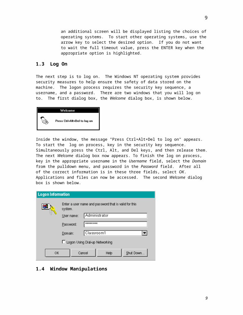
The next step is to log on. The Windows NT operating system provides security measures to help ensure the safety of data stored on the machine. The logon process requires the security key sequence, a username, and a password. There are two windows that you will log on to. The first dialog box, the Welcome dialog box, is shown below.
6
6
Inside the window, the message "Press Ctrl+Alt+Del to log on" appears. To start the log on process, key in the security key sequence. Simultaneously press the Ctrl, Alt, and Del keys, and then release them. The next Welcome dialog box now appears. To finish the log on process, key in the appropriate username in the Username field, select the Domain from the pulldown menu, and password in the Password field. After all of the correct information is in these three fields, select OK. Applications and files can now be accessed. The second Welcome dialog box is shown below.
1.4 Window Manipulations
Most work in the Windows NT operating system is carried out by using a window and menu interface. Therefore, it is necessary to understand how to manipulate windows. After completing this lesson, you will be able to perform many different window manipulations.
In these sections you will be able to do the following:
Identify Window Components
Manipulate Windows
Use Pulldown Menus
Use Dialog Boxes
1.4.1 Window Components and Sizing
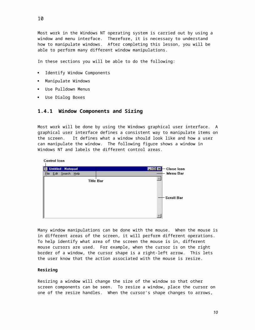
Most work will be done by using the Windows graphical user interface. A graphical user interface defines a consistent way to manipulate items on the screen. It defines what a window should look like and how a user can manipulate the window. The following figure shows a window in Windows NT and labels the different control areas.
7
7
Many window manipulations can be done with the mouse. When the mouse is in different areas of the screen, it will perform different operations. To help identify what area of the screen the mouse is in, different mouse cursors are used. For example, when the cursor is on the right border of a window, the cursor shape is a right-left arrow. This lets the user know that the action associated with the mouse is resize.
Resizing
Resizing a window will change the size of the window so that other screen components can be seen. To resize a window, place the cursor on one of the resize handles. When the cursor's shape changes to arrows, press and hold the mouse button, drag the mouse to the desired location, and release the mouse button.
Move
Moving a window will change the location of a window so that other screen components can be seen. To move a window, place the cursor on the title bar, press and hold the mouse, drag the mouse to the desired location, and release the mouse. To move a minimized window, press and hold the mouse button on the icon, drag the mouse to the desired location, and release the mouse button.
Minimize Minimizing a window will change the shape of the window to be a small icon on the screen. A minimized window takes up a small amount of screen area without deleting the window. To minimize a window, select the minimize icon. The window will now be displayed as an icon. By default, icons are arranged on the bottom of the screen.Restore Minimized
Restoring a minimized window will give you access to the window. To restore a minimized window, double click on the icon. The following figure shows the Clock as a minimized window, and the Notepad and Program Manager applications as regular windows.
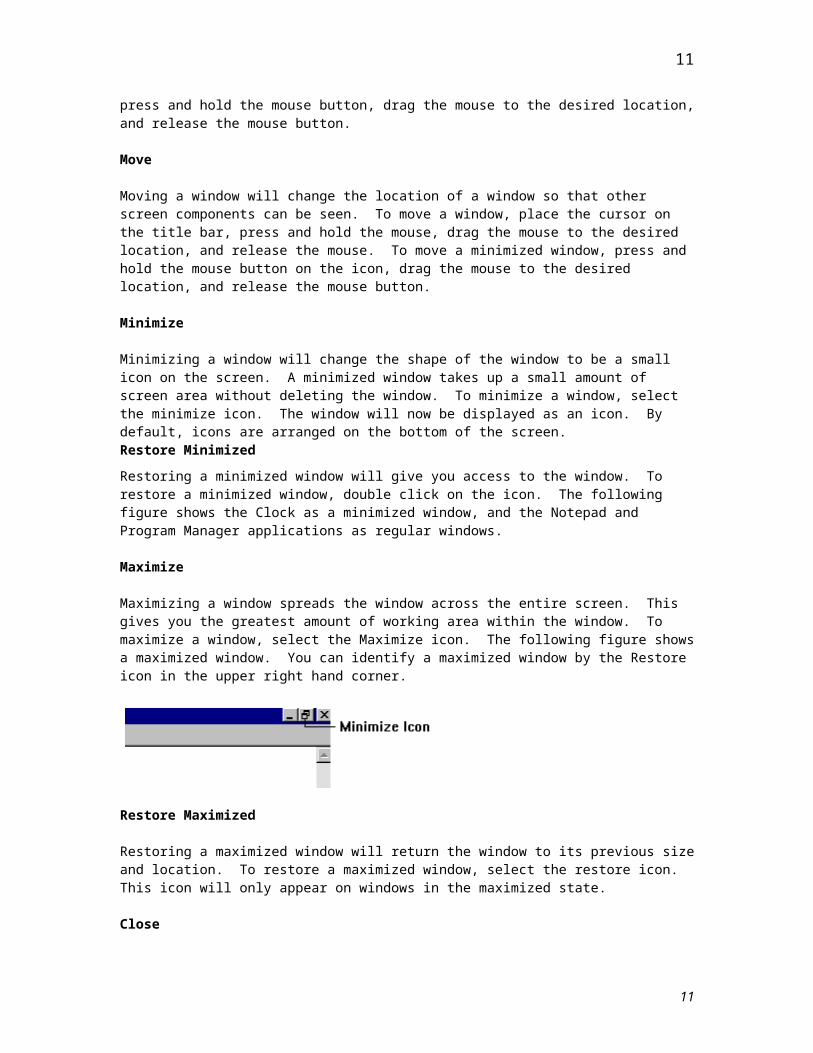
Maximize
Maximizing a window spreads the window across the entire screen. This gives you the greatest amount of working area within the window. To maximize a window, select the Maximize icon. The following figure shows a maximized window. You can identify a maximized window by the Restore icon in the upper right hand corner.
8
8
Restore Maximized
Restoring a maximized window will return the window to its previous size and location. To restore a maximized window, select the restore icon. This icon will only appear on windows in the maximized state.
Close
Closing a window will delete it from the screen. This will clean up the screen by eliminating unused windows. To close a window, double click on the Control Menu icon. It will not delete information from the hard disk.
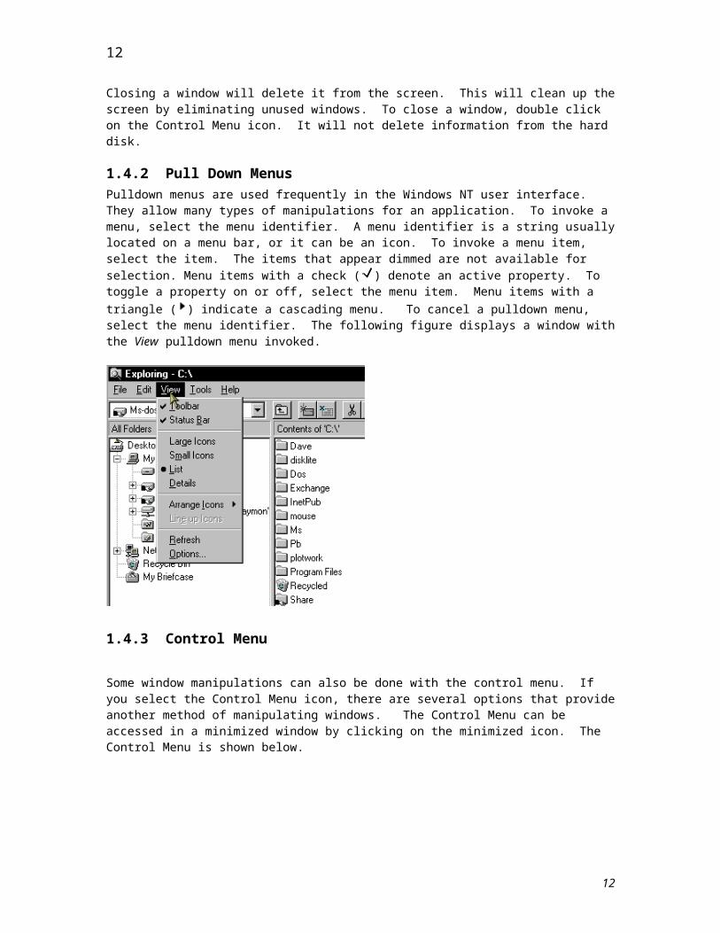
1.4.2 Pull Down MenusPulldown menus are used frequently in the Windows NT user interface. They allow many types of manipulations for an application. To invoke a menu, select the menu identifier. A menu identifier is a string usually located on a menu bar, or it can be an icon. To invoke a menu item, select the item. The items that appear dimmed are not available for selection. Menu items with a check ( ) denote an active property. To toggle a property on or off, select the menu item. Menu items with a triangle ( ) indicate a cascading menu. To cancel a pulldown menu, select the menu identifier. The following figure displays a window with the View pulldown menu invoked.
1.4.3 Control Menu
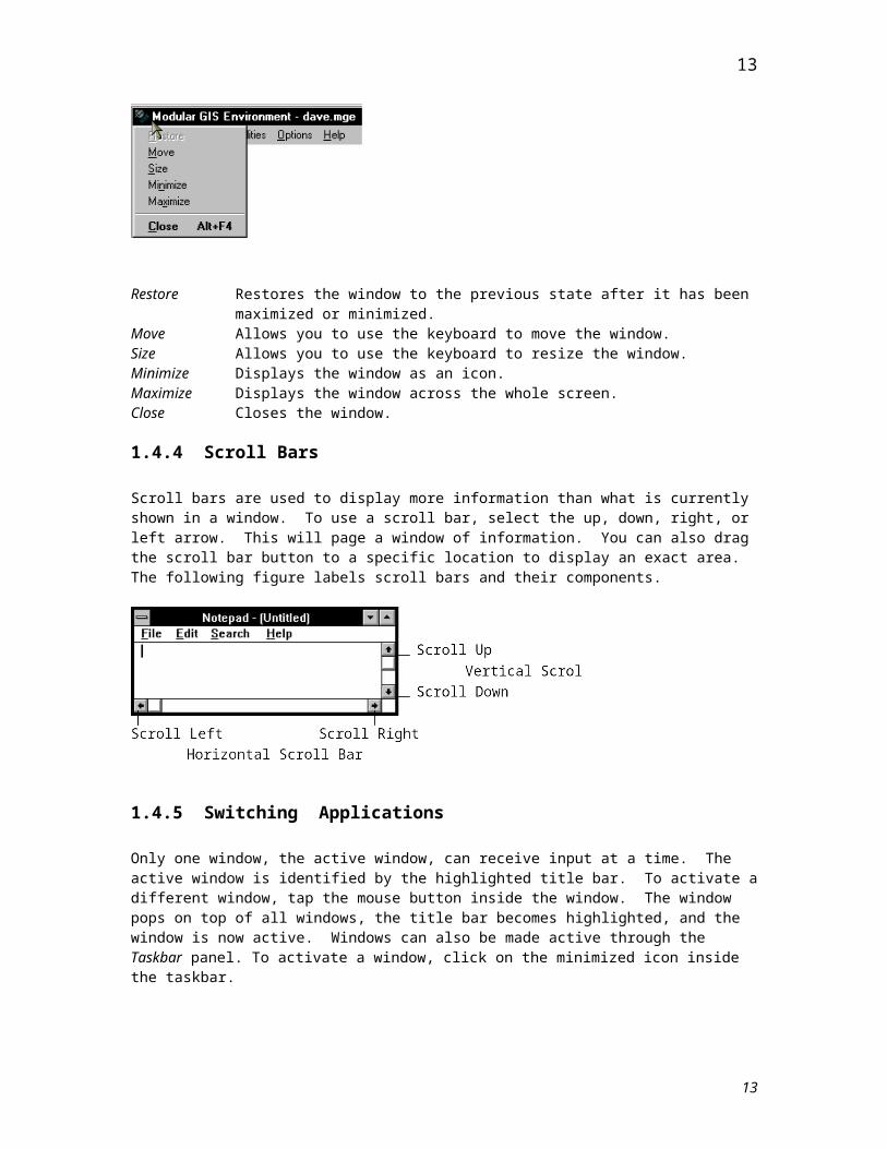
Some window manipulations can also be done with the control menu. If you select the Control Menu icon, there are several options that provide another method of manipulating windows. The Control Menu can be accessed in a minimized window by clicking on the minimized icon. The Control Menu is shown below.
9
9
Restore Restores the window to the previous state after it has been maximized or minimized. Move Allows you to use the keyboard to move the window.Size Allows you to use the keyboard to resize the window.Minimize Displays the window as an icon.Maximize Displays the window across the whole screen.Close Closes the window.
1.4.4 Scroll Bars
Scroll bars are used to display more information than what is currently shown in a window. To use a scroll bar, select the up, down, right, or left arrow. This will page a window of information. You can also drag the scroll bar button to a specific location to display an exact area. The following figure labels scroll bars and their components.
1.4.5 Switching Applications
Only one window, the active window, can receive input at a time. The active window is identified by the highlighted title bar. To activate a different window, tap the mouse button inside the window. The window pops on top of all windows, the title bar becomes highlighted, and the window is now active. Windows can also be made active through the Taskbar panel. To activate a window, click on the minimized icon inside the taskbar.
10
10
Lesson 2 - The Windows Desktop
The Desktop is your working screen area - you may create or manipulate windows, icons and dialog boxes on your desktop.
After completing this lesson, you will be able to do the following:
Create ShortcutsManipulate and Modify ShortcutsSet Passwords on AccountsLog Off, Restart, and Shut Down the System
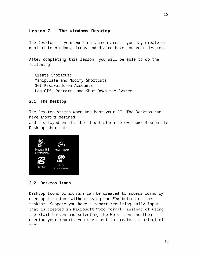
2.1 The Desktop
The Desktop starts when you boot your PC. The Desktop can have shortcuts definedand displayed on it. The illustration below shows 4 separate Desktop shortcuts.
2.2 Desktop Icons
Desktop Icons or shortcuts can be created to access commonly used applications without using the Start button on the taskbar. Suppose you have a report requiring daily input that is created in Microsoft Word format, instead of using the Start button and selecting the Word icon and then opening your report, you may elect to create a shortcut of thedocument on your desktop - thus saving yourself 2 extra steps needed to open the desired document.
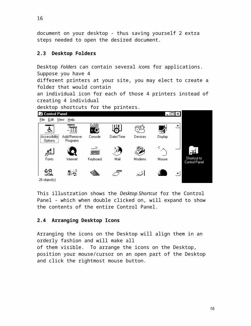
2.3 Desktop Folders
Desktop Folders can contain several icons for applications. Suppose you have 4different printers at your site, you may elect to create a folder that would containan individual icon for each of those 4 printers instead of creating 4 individualdesktop shortcuts for the printers.
11
11
This illustration shows the Desktop Shortcut for the Control Panel - which when double clicked on, will expand to show the contents of the entire Control Panel.
2.4 Arranging Desktop Icons
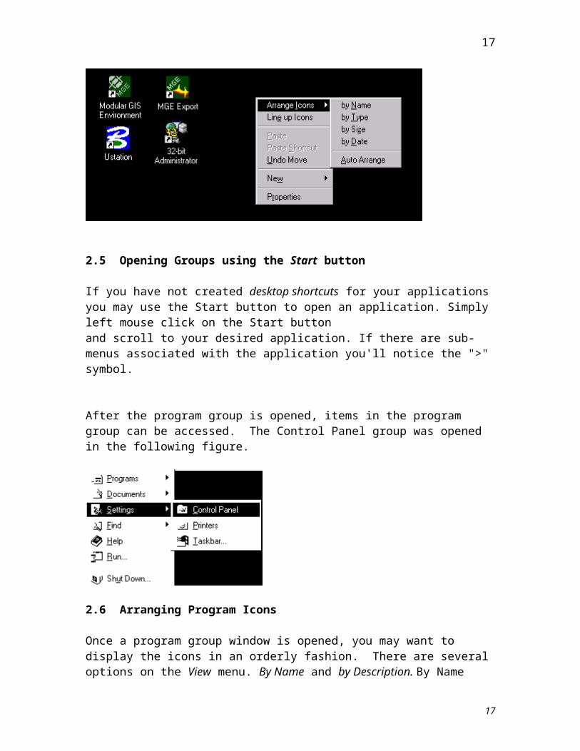
Arranging the icons on the Desktop will align them in an orderly fashion and will make all of them visible. To arrange the icons on the Desktop, position your mouse/cursor on an open part of the Desktop and click the rightmost mouse button.
2.5 Opening Groups using the Start button
If you have not created desktop shortcuts for your applications you may use the Start button to open an application. Simply left mouse click on the Start buttonand scroll to your desired application. If there are sub-menus associated with the application you'll notice the ">" symbol.
12
12
After the program group is opened, items in the program group can be accessed. The Control Panel group was opened in the following figure.
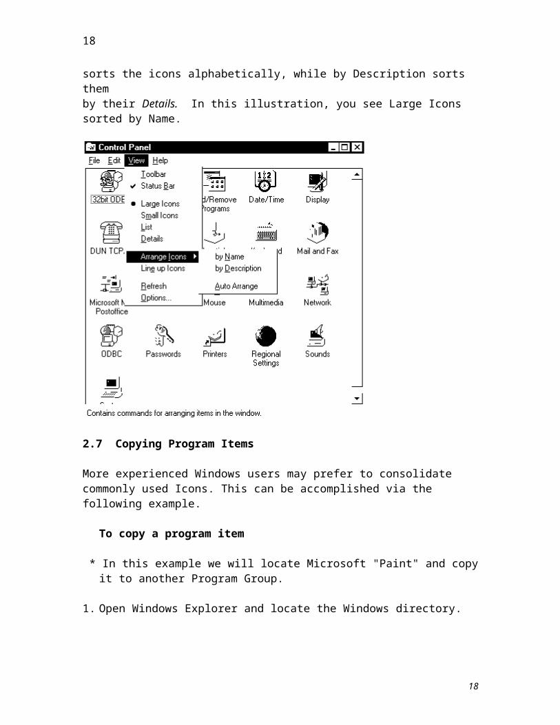
2.6 Arranging Program Icons
Once a program group window is opened, you may want to display the icons in an orderly fashion. There are several options on the View menu. By Name and by Description. By Name sorts the icons alphabetically, while by Description sorts themby their Details. In this illustration, you see Large Icons sorted by Name.
2.7 Copying Program Items
13
13

More experienced Windows users may prefer to consolidate commonly used Icons. This can be accomplished via the following example.
To copy a program item * In this example we will locate Microsoft "Paint" and copy it to another Program
Group.
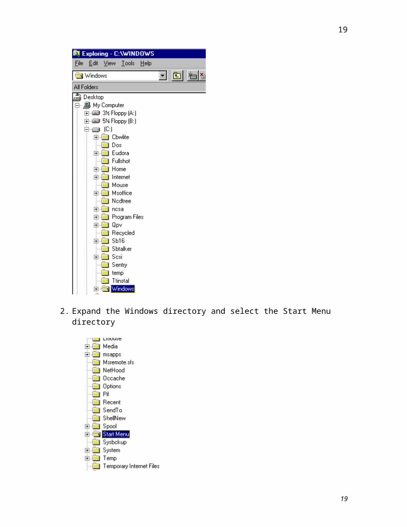
1. Open Windows Explorer and locate the Windows directory.
2. Expand the Windows directory and select the Start Menu directory
14
14
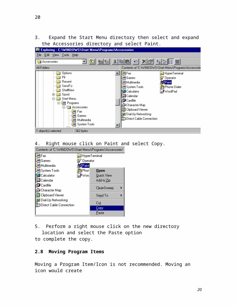
3. Expand the Start Menu directory then select and expand the Accessories directory and select Paint.
4. Right mouse click on Paint and select Copy.
15
15
5. Perform a right mouse click on the new directory location and select the Paste optionto complete the copy.
2.8 Moving Program Items
Moving a Program Item/Icon is not recommended. Moving an icon would createa mismatch in the system registry and render the program useless.
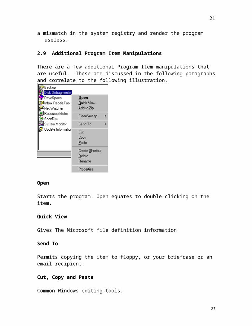
2.9 Additional Program Item Manipulations
There are a few additional Program Item manipulations that are useful. These are discussed in the following paragraphs and correlate to the following illustration.
Open
Starts the program. Open equates to double clicking on the item.
16
16
Quick View
Gives The Microsoft file definition information
Send To
Permits copying the item to floppy, or your briefcase or an email recipient.
Cut, Copy and Paste
Common Windows editing tools.
Create Shortcut - Delete - Rename
Create Shortcut creates a copy of the Item, while Delete will place the item in theRecycle Bin, and Rename will allow renaming of the item.
Properties
Displays general and shortcut information.
2.10 Creating a Personal Desktop Folder
A Personal Desktop Folder can contain shortcuts to commonly used applications, eliminating the need to select the application from the Start Taskbar.
To add a new program group
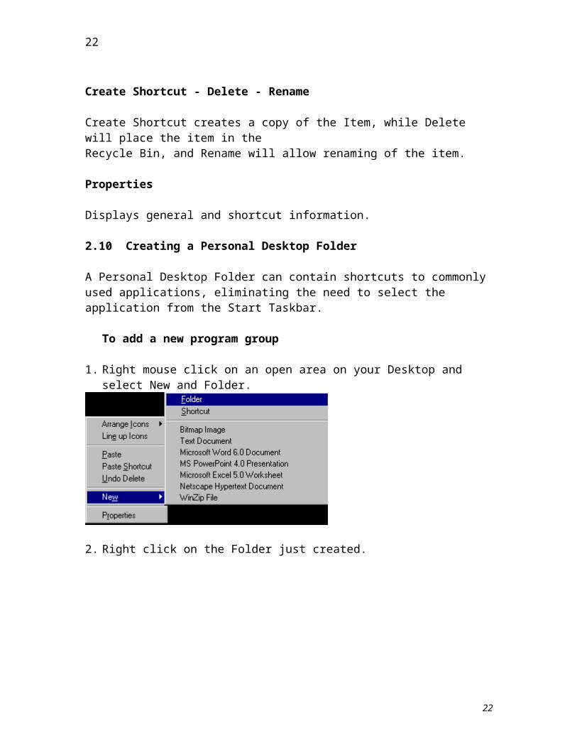
1. Right mouse click on an open area on your Desktop and select New and Folder.
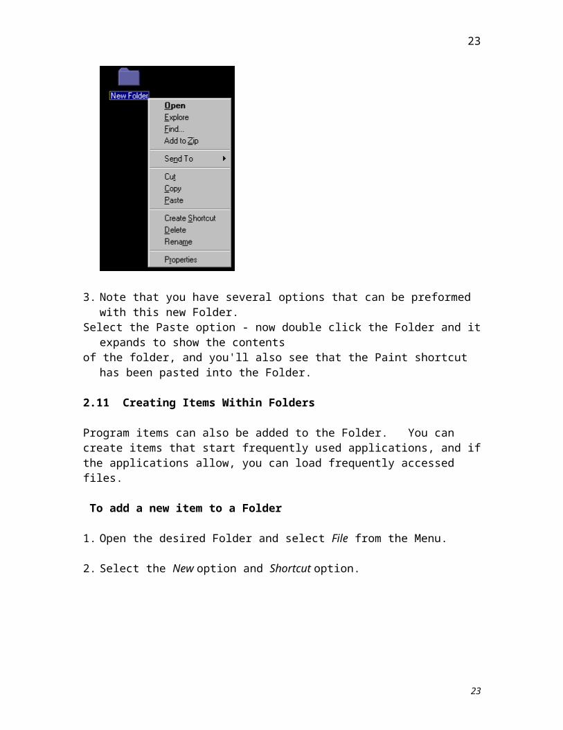
2. Right click on the Folder just created.
17
17
3. Note that you have several options that can be preformed with this new Folder.Select the Paste option - now double click the Folder and it expands to show the contentsof the folder, and you'll also see that the Paint shortcut has been pasted into the Folder.
2.11 Creating Items Within Folders
Program items can also be added to the Folder. You can create items that start frequently used applications, and if the applications allow, you can load frequently accessed files.
To add a new item to a Folder
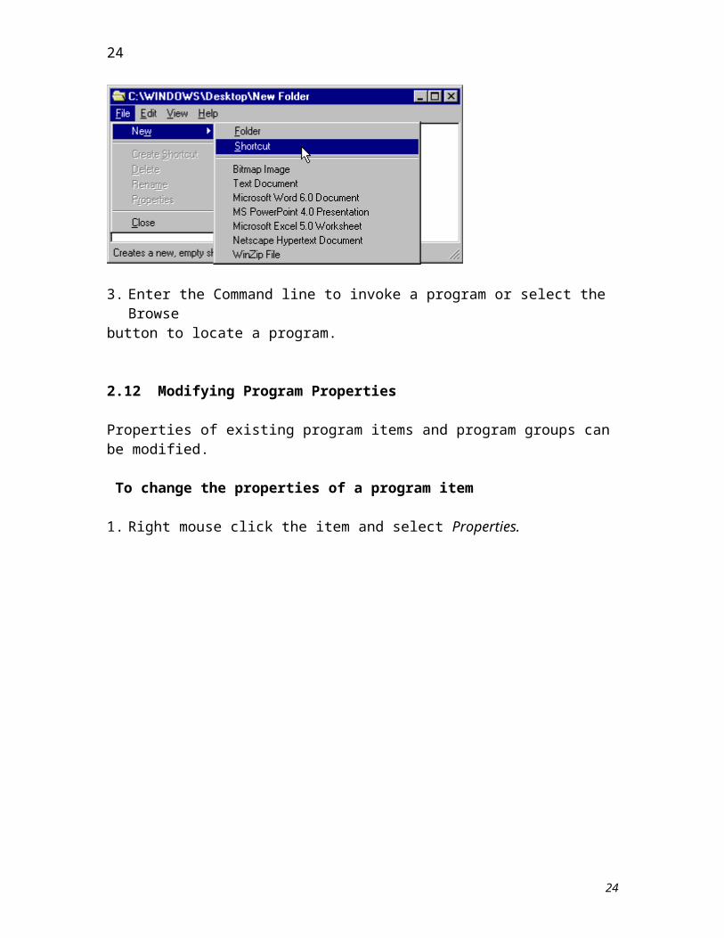
1. Open the desired Folder and select File from the Menu.
2. Select the New option and Shortcut option.
3. Enter the Command line to invoke a program or select the Browse
18
18
button to locate a program.
2.12 Modifying Program Properties
Properties of existing program items and program groups can be modified.
To change the properties of a program item
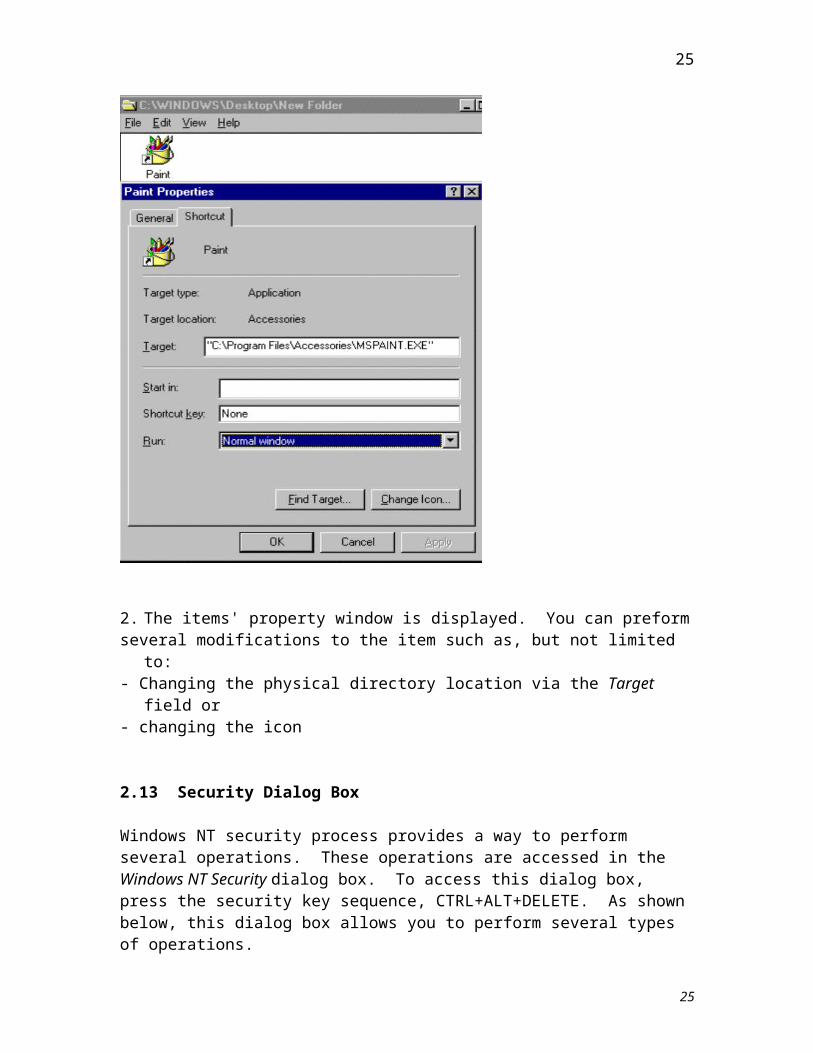
1. Right mouse click the item and select Properties.
2. The items' property window is displayed. You can preformseveral modifications to the item such as, but not limited to:- Changing the physical directory location via the Target field or- changing the icon
2.13 Security Dialog Box
19
19
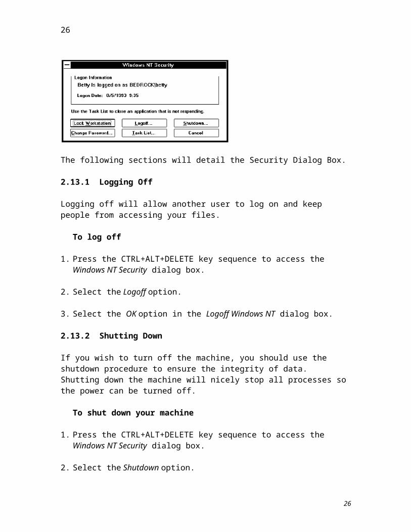
Windows NT security process provides a way to perform several operations. These operations are accessed in the Windows NT Security dialog box. To access this dialog box, press the security key sequence, CTRL+ALT+DELETE. As shown below, this dialog box allows you to perform several types of operations.
The following sections will detail the Security Dialog Box.
2.13.1 Logging Off
Logging off will allow another user to log on and keep people from accessing your files.
To log off
1. Press the CTRL+ALT+DELETE key sequence to access the Windows NT Security dialog box.
2. Select the Logoff option.
3. Select the OK option in the Logoff Windows NT dialog box.
2.13.2 Shutting Down
If you wish to turn off the machine, you should use the shutdown procedure to ensure the integrity of data. Shutting down the machine will nicely stop all processes so the power can be turned off.
To shut down your machine
1. Press the CTRL+ALT+DELETE key sequence to access the Windows NT Security dialog box.
2. Select the Shutdown option.
3. Select OK in the Shutdown Computer dialog box.
20
20
4. When the It is safe to turn off your computer dialog box is displayed, the power switch can be turned off.
2.13.3 Restarting
When system settings have changed, you will need to restart the computer so the operating system initializes the new settings. Restarting your machine will close all files, stop all processes, and reinitialize the operating system.
To restart your machine
1. Press the CTRL+ALT+DELETE key sequence to access the Windows NT Security dialog box.
2. Select the Shutdown option.
3. Check the Restart Computer option in the Shutdown Computer dialog box.
4. Select OK in the Shutdown Computer dialog box.
2.13.4 Changing Your Password
As a security measure, each user account can have a password to protect the machine and the files that reside on it.
To change your password
1. Press the CTRL+ALT+DELETE key sequence to access the Windows NT Security dialog box.
2. Select the Change Password option.
3. The Change Password dialog box appears. Key in your old password in the Old Password field.
4. Key in the new password in the Password and Confirm New Password fields.
21
21
Lesson 3 - Windows Explorer
Explorer is an application that allows you to manage files on the system.
After completing this lesson, you will be able to perform the following functions within the Explorer environment:
Manipulate Files
View Various Types of Drives
Perform Floppy Operations
Modify Viewing Parameters
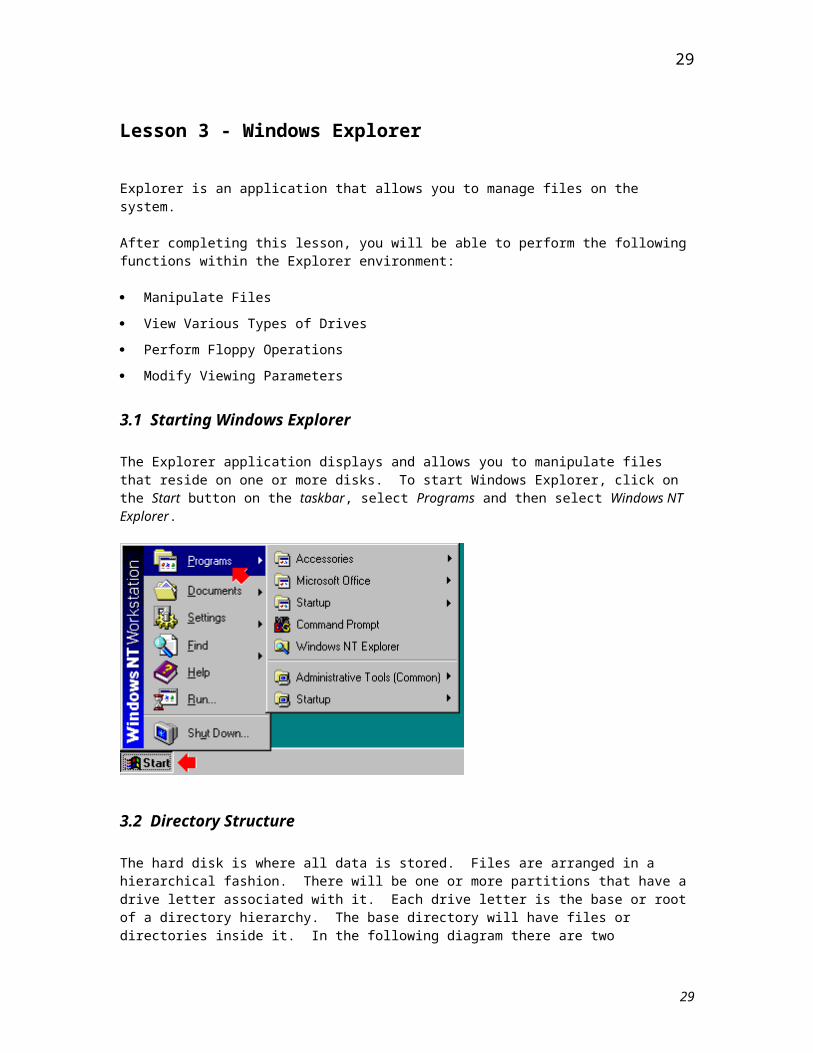
3.1 Starting Windows Explorer
The Explorer application displays and allows you to manipulate files that reside on one or more disks. To start Windows Explorer, click on the Start button on the taskbar, select Programs and then select Windows NT Explorer.
3.2 Directory Structure
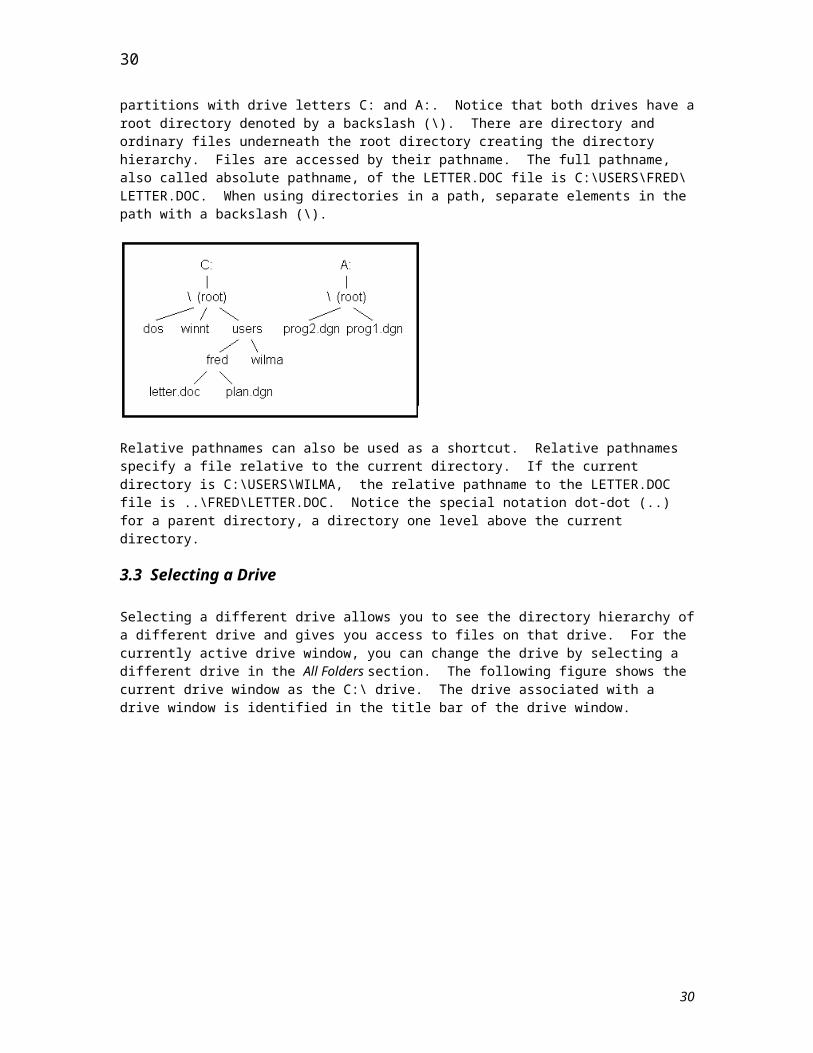
The hard disk is where all data is stored. Files are arranged in a hierarchical fashion. There will be one or more partitions that have a drive letter associated with it. Each drive letter is the base or root of a directory hierarchy. The base directory will have files or directories inside it. In the following diagram there are two partitions with drive letters C: and A:. Notice that both drives have a root directory denoted by a backslash (\). There are directory and ordinary files underneath the root directory creating the directory hierarchy. Files are accessed by their pathname. The full pathname, also called absolute pathname, of the LETTER.DOC file is C:\USERS\FRED\LETTER.DOC. When using directories in a path, separate elements in the path with a backslash (\).
22
22
Relative pathnames can also be used as a shortcut. Relative pathnames specify a file relative to the current directory. If the current directory is C:\USERS\WILMA, the relative pathname to the LETTER.DOC file is ..\FRED\LETTER.DOC. Notice the special notation dot-dot (..) for a parent directory, a directory one level above the current directory.
3.3 Selecting a Drive
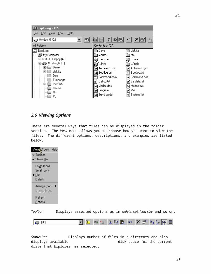
Selecting a different drive allows you to see the directory hierarchy of a different drive and gives you access to files on that drive. For the currently active drive window, you can change the drive by selecting a different drive in the All Folders section. The following figure shows the current drive window as the C:\ drive. The drive associated with a drive window is identified in the title bar of the drive window.
3.6 Viewing Options
There are several ways that files can be displayed in the folder section. The View menu allows you to choose how you want to view the files. The different options, descriptions, and examples are listed below.
23
23
Toolbar Displays assorted options as in delete, cut, icon size and so on.
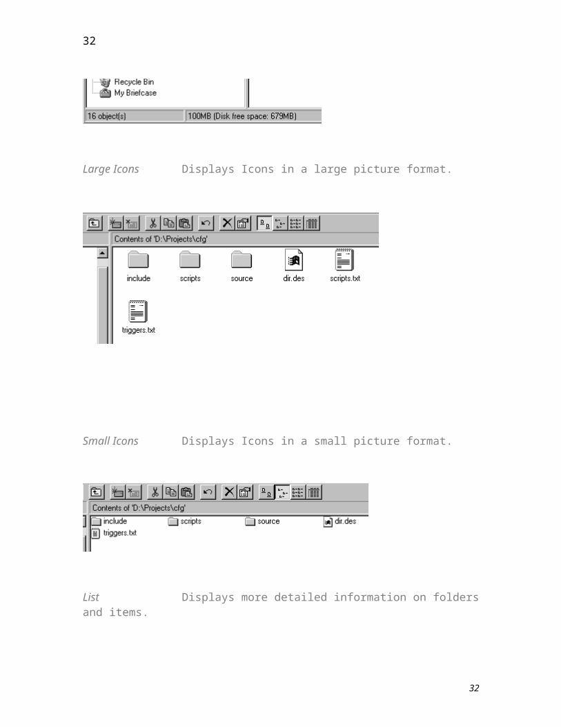
Status Bar Displays number of files in a directory and also displays available disk space for the current drive that Explorer has selected.
Large Icons Displays Icons in a large picture format.
24
24
Small Icons Displays Icons in a small picture format.
List Displays more detailed information on folders and items.
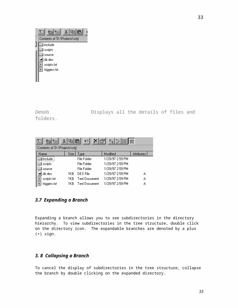
Details Displays all the details of files and folders.
25
25
3.7 Expanding a Branch
Expanding a branch allows you to see subdirectories in the directory hierarchy. To view subdirectories in the tree structure, double click on the directory icon. The expandable branches are denoted by a plus (+) sign.
3. 8 Collapsing a Branch
To cancel the display of subdirectories in the tree structure, collapse the branch by double clicking on the expanded directory.
3.9 File Naming Conventions
For standard DOS files there is a set of rules that must be adhered to when naming files. The rules are as follows:
Must not have more than eight characters, and no more than a three character extension.
Must contain alphanumeric or the following special characters:
_ ^ $ ~ ! # % & - { } ( ) @ ' `
Must not contain spaces, commas, backslashes, or periods (a period in the extension is acceptable).
For FAT (file allocation table) file systems allows you to have files with up to an 8 character name, and 3 character extension.
For NTFS (NT) file system you can have filenames of up to 254 characters.
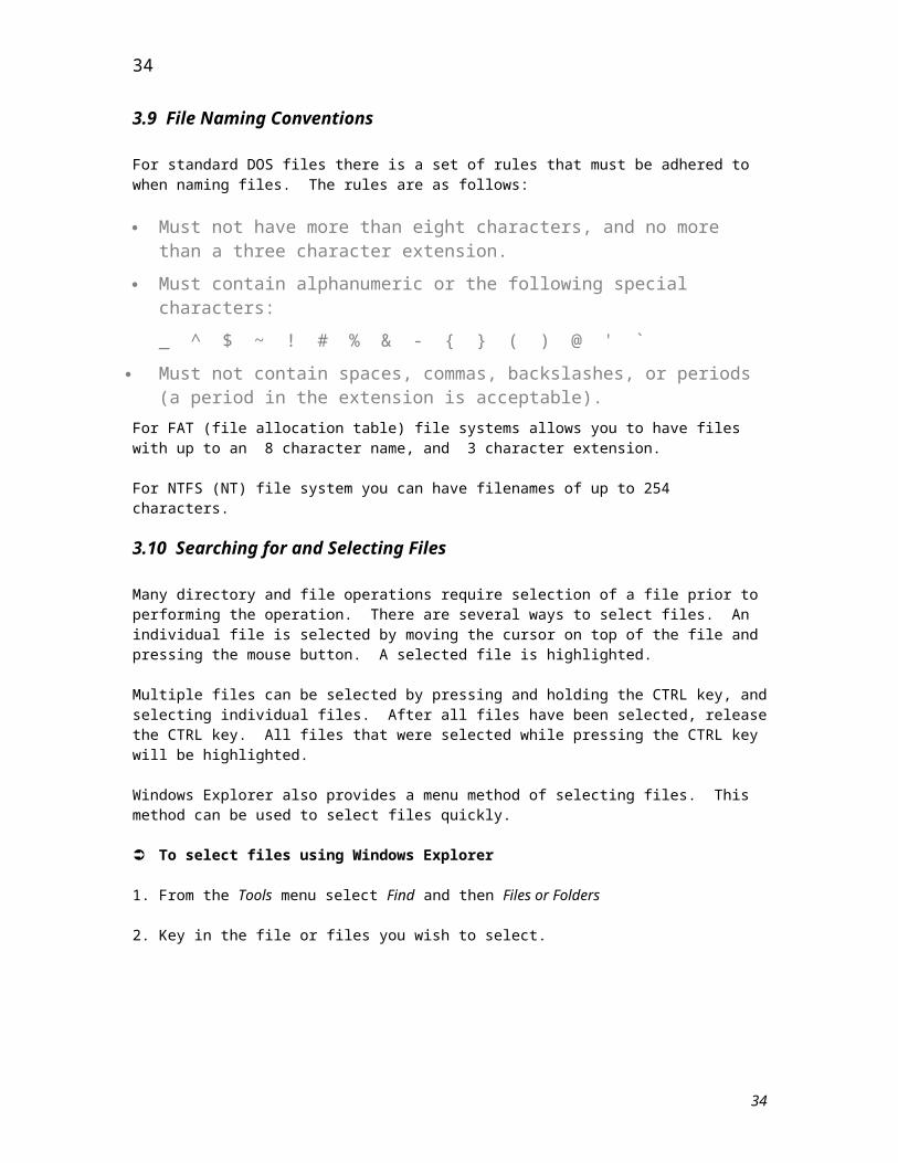
3.10 Searching for and Selecting Files
Many directory and file operations require selection of a file prior to performing the operation. There are several ways to select files. An individual file is selected by moving the cursor on top of the file and pressing the mouse button. A selected file is highlighted. Multiple files can be selected by pressing and holding the CTRL key, and selecting individual files. After all files have been selected, release the CTRL key. All files that were selected while pressing the CTRL key will be highlighted.
Windows Explorer also provides a menu method of selecting files. This method can be used to select files quickly.
Ü To select files using Windows Explorer
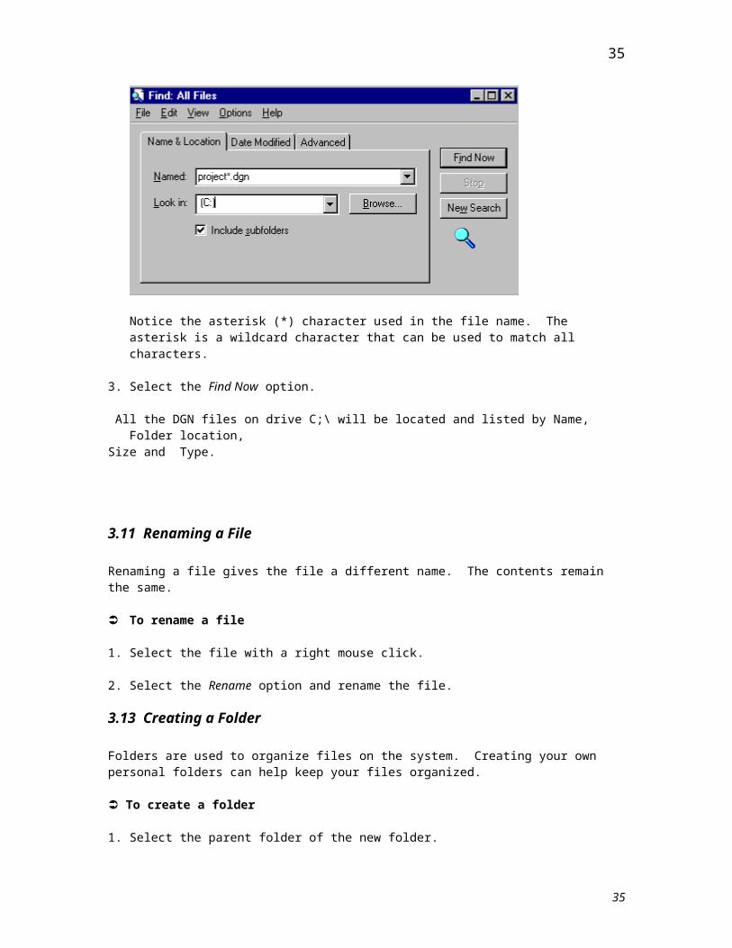
1. From the Tools menu select Find and then Files or Folders
2. Key in the file or files you wish to select.
26
26
Notice the asterisk (*) character used in the file name. The asterisk is a wildcard character that can be used to match all characters.
3. Select the Find Now option.
All the DGN files on drive C;\ will be located and listed by Name, Folder location,Size and Type.
3.11 Renaming a File
Renaming a file gives the file a different name. The contents remain the same.
Ü To rename a file
1. Select the file with a right mouse click.
2. Select the Rename option and rename the file.
3.13 Creating a Folder
Folders are used to organize files on the system. Creating your own personal folders can help keep your files organized.
Ü To create a folder
1. Select the parent folder of the new folder.
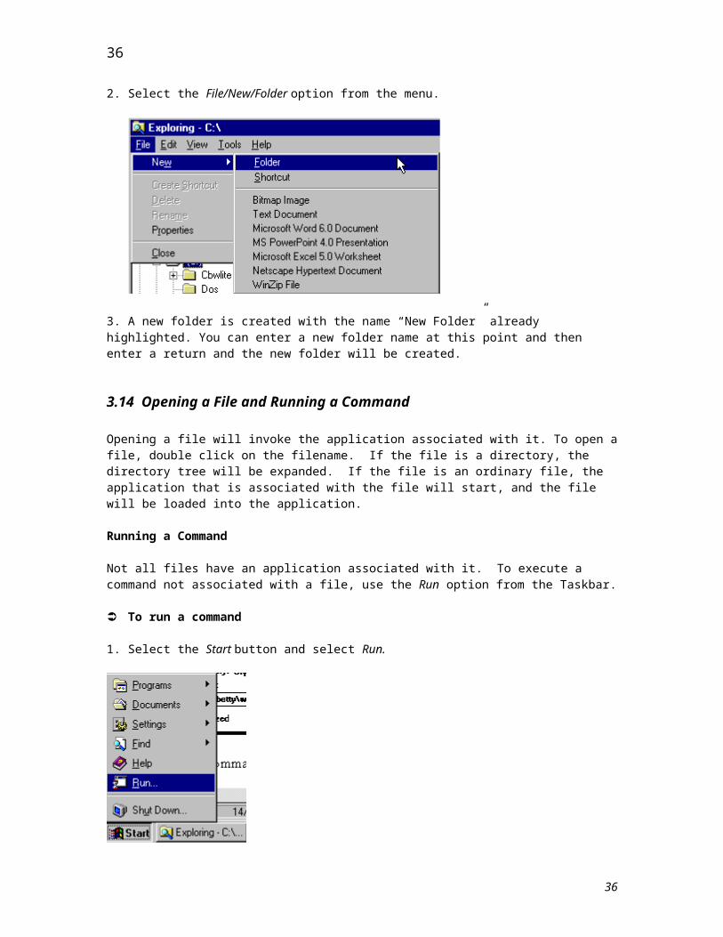
2. Select the File/New/Folder option from the menu.
27
27

3. A new folder is created with the name “New Folder” alreadyhighlighted. You can enter a new folder name at this point and thenenter a return and the new folder will be created.
3.14 Opening a File and Running a Command
Opening a file will invoke the application associated with it. To open a file, double click on the filename. If the file is a directory, the directory tree will be expanded. If the file is an ordinary file, the application that is associated with the file will start, and the file will be loaded into the application.
Running a Command
Not all files have an application associated with it. To execute a command not associated with a file, use the Run option from the Taskbar.
Ü To run a command
1. Select the Start button and select Run.
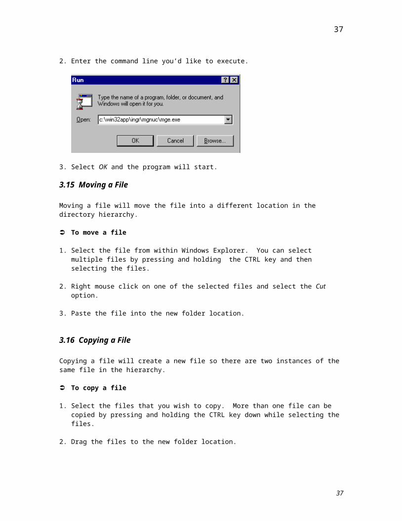
2. Enter the command line you’d like to execute.
28
28
3. Select OK and the program will start.
3.15 Moving a File
Moving a file will move the file into a different location in the directory hierarchy.
Ü To move a file
1. Select the file from within Windows Explorer. You can select multiple files by pressing and holding the CTRL key and then selecting the files.
2. Right mouse click on one of the selected files and select the Cut option.
3. Paste the file into the new folder location.
3.16 Copying a File
Copying a file will create a new file so there are two instances of the same file in the hierarchy.
Ü To copy a file
1. Select the files that you wish to copy. More than one file can be copied by pressing and holding the CTRL key down while selecting the files.
2. Drag the files to the new folder location.
3.17 Deleting a File
Deleting a file will remove it from the hard disk. This operation is used to get rid of unused files to free up space for new files.
Ü To delete a file
1. Select the files that you wish to delete. More than one file can be deleted by pressing and holding the CTRL key down while selecting the files.
2. Select the File option from the menu and select Delete.
3. Confirm or deny the deletion.
29
29
3.18 Editing a File
The Notepad or Wordpad editor will allow you to edit text files. Either application will run under Windows on MS-DOS and Windows NT.
Ü To start the Notepad editor
1. Select the Notepad icon from the Accessories program group.
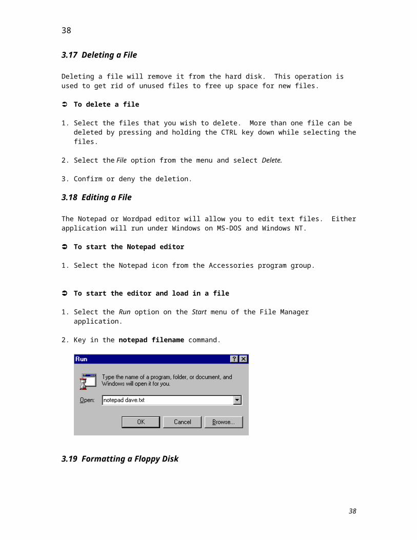
Ü To start the editor and load in a file
1. Select the Run option on the Start menu of the File Manager application.
2. Key in the notepad filename command.
3.19 Formatting a Floppy Disk
In order to place information on a floppy disk, it must first be initialized. This is done by formatting the floppy disk.
Ü To format a floppy disk
1. Place a floppy in the floppy disk drive.
2. Right mouse click on the A drive within Windows Explorer and
select Format.
Ü To copy files to a floppy disk
1. Place a formatted floppy in the floppy drive.
2. Select the file(s) you want to copy and drag them to the Drive A folder within Windows Explorer.
3.20 Copying a Floppy Disk
Copying a floppy transfers all information from one floppy to another. All information on the destination floppy will be overwritten.
30
30
Ü To copy a floppy to another floppy
1. Select the Drive A folder with a right mouse click, then select Copy Disk.
2. Follow the system prompts to complete the copy.
3.21 Connecting to a Network Drive
A network share can be created on a machine that has files that users on other machines need to access. Your system administrator can create a network share. Once a share is created, a node on the network can create a network drive to the share.
Ü To connect to a network drive
1. Select the Tools menu from Windows Explorer.
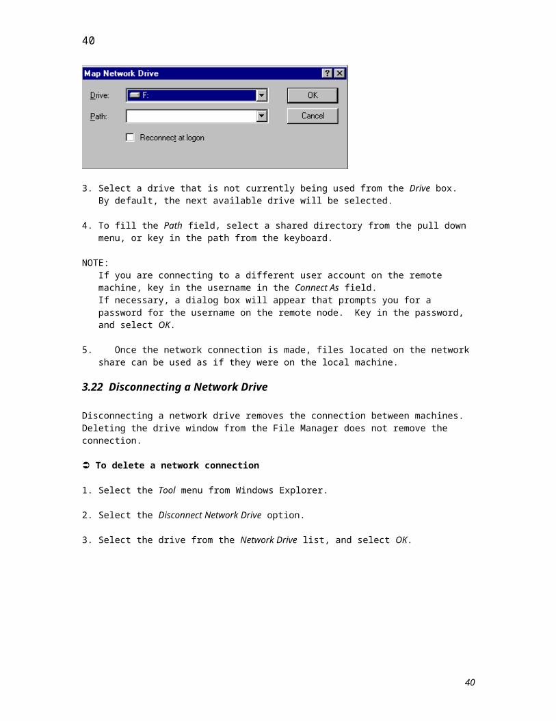
2. Select the Map Network Drive option. The Map Network Drive dialog box appears.
3. Select a drive that is not currently being used from the Drive box. By default, the next available drive will be selected.
4. To fill the Path field, select a shared directory from the pull down menu, or key in the path from the keyboard.
NOTE:If you are connecting to a different user account on the remote machine, key in the username in the Connect As field.If necessary, a dialog box will appear that prompts you for a password for the username on the remote node. Key in the password, and select OK.
5. Once the network connection is made, files located on the network share can be used as if they were on the local machine.
3.22 Disconnecting a Network Drive
Disconnecting a network drive removes the connection between machines. Deleting the drive window from the File Manager does not remove the connection.
Ü To delete a network connection
1. Select the Tool menu from Windows Explorer.
31
31
2. Select the Disconnect Network Drive option.
3. Select the drive from the Network Drive list, and select OK.
32
32
Lesson 4 - Customizing the Environment
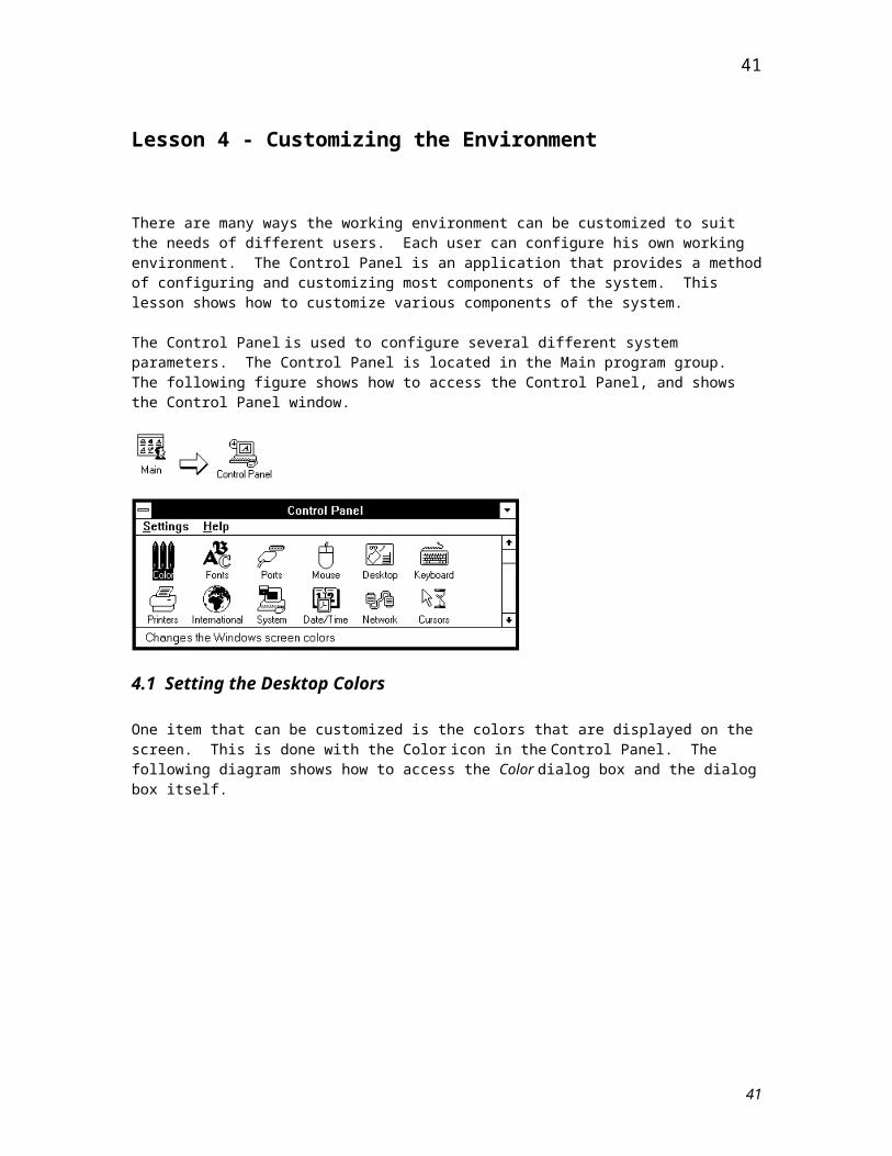
There are many ways the working environment can be customized to suit the needs of different users. Each user can configure his own working environment. The Control Panel is an application that provides a method of configuring and customizing most components of the system. This lesson shows how to customize various components of the system.
The Control Panel is used to configure several different system parameters. The Control Panel is located in the Main program group. The following figure shows how to access the Control Panel, and shows the Control Panel window.
4.1 Setting the Desktop Colors
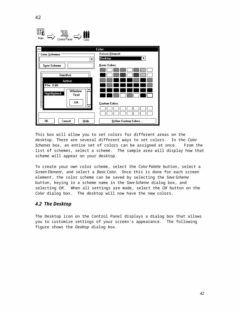
One item that can be customized is the colors that are displayed on the screen. This is done with the Color icon in the Control Panel. The following diagram shows how to access the Color dialog box and the dialog box itself.
33
33
This box will allow you to set colors for different areas on the desktop. There are several different ways to set colors. In the Color Schemes box, an entire set of colors can be assigned at once. From the list of schemes, select a scheme. The sample area will display how that scheme will appear on your desktop.
To create your own color scheme, select the Color Palette button, select a Screen Element, and select a Basic Color. Once this is done for each screen element, the color scheme can be saved by selecting the Save Scheme button, keying in a scheme name in the Save Scheme dialog box, and selecting OK. When all settings are made, select the OK button on the Color dialog box. The desktop will now have the new colors.
4.2 The Desktop
The Desktop icon on the Control Panel displays a dialog box that allows you to customize settings of your screen's appearance. The following figure shows the Desktop dialog box.
34
34
The Pattern option sets your desktop pattern. The pattern will be displayed as the background for the screen.
When Fast Alt+Tab Switching is turned on, you can switch between applications quickly. To use this feature, press and hold the ALT key, press and release the TAB key until the desired application is listed, and release the ALT key.
A Screen Saver can be turned on by selecting one from the list setting the delay time. Most screen savers can be configured from the Setup button. Screen savers can also be tested quickly by selecting the Test button.
When the Password Protected box is turned on, the user must press the CTRL+ALT+DELETE key sequence, and then key in the password to regain access the system.A wallpaper can be displayed on the background screen by selecting a wallpaper from the File list in the Wallpaper box. The Center option will display one copy of the pattern in the center of the screen. The Tile option will tile the pattern over the entire screen.
In the Sizing Grid box, the granularity and the border width can be set. The Granularity option sets a grid that determines the arrangement of windows and icons. The Border Width field sets the border width of windows.
In the Icons box, the spacing of icons and the Wrap Title option can be set. The Spacing option determines how far away icons are spaced. When the Wrap Title is turned on, the icon descriptions will wrap around to another line.
To set the text cursor blinking speed, move the scroll bar in the Cursor Blink Rate box.
4.3 Cursors
35
35
Cursors that are associated with defined operations can be changed in the Cursors icon in the Control Panel. To change a cursor, in the Cursors dialog box select the cursor in the System Cursors list, select the Browse button, select the file from the File Name list, and select OK in the Browse dialog box. A different icon can be selected for each item in the System Cursors list. The following figure shows the Cursors dialog box.
36
36
Lesson 5 - The Design File
In order to use MicroStation effectively, you must understand a few fundamental concepts about design files.
The following concepts will be discussed in this lesson:
Explain the concept of a design plane. File Entry, Microstation Manager and File Utilities Graphics Interface Seed File Properly save and exit a design file.
5.1 The Design Plane
The MicroStation design plane is similar to the paper you would use for manual drafting because, like the paper, it has certain limits that you can not exceed. The design plane is divided into a grid that has 4,294,967,296 divisions. Each of these divisions is a possible position for a point on an element. Each point in the design plane has associated horizontal and vertical positions or coordinates. So, the design plane is actually a coordinate system that you draw your design in.
5.2 File Entry
Entry into map files is facilitated through Microstation Manager. Microstation Manager is accessed from the Microstation 95 Common Window by clicking on the Microstation 95 icon.
There are two Menu items to choose from File and Directory. The items under File are:
New - This item displays the Create Design File dialog box. It can be used to create design files. This dialog box is explained in more detail on the following pages.
37
37
Copy - You can use this item to copy a file. By default, the current file will display as the From file and the current filename with a .bak extension will display as the To file in the Copy dialog box that displays when you select this item.
Rename - This item brings up the Rename dialog box and allows you to rename a file. By default, you will be renaming the current file. You can type in any new name for this file in the To data entry box.
Delete - When you select this item, you are indicating that you want to delete the current file. An alert box will display and force you to confirm this action.
Compress - You can select this item to compress the current file. An information box will display when the compression is complete.
Numbered Items - The filenames listed beside the numbers are the names of the last files that you attempted to open in MicroStation. If you select one of these items, the associated file will be opened in MicroStation.
Exit - This item will exit the MicroStation Manager interface.
There are several components to the graphical user interface for Microstation in a mapping environment. Discussed will be the following:
Command Window Setting Box Tool Palette Main Palette
Command Window
The Command Window is the command center for MicroStation. This window shows which design file is currently active, it contains the menu bar used to access all the MicroStation menus, and it displays the active tool, the active status parameters, and error messages. The Command Window also prompts you to provide any input necessary for performance of the active tool. Closing this window indicates that you wish to exit MicroStation.
The six fields below the menu bar are:
Status - Displays notices about changes to current settings or locks. Message - Displays current element parameter settings. Command - Displays the name of the active drawing tool. Prompt - Displays the next user operation needed by Microstation. Input - Displays keyboard input for validating typed entries. Error - Displays error messages.
38
38
Command Field
Input Field
Status Field
Prompt Field
Error Field Message Field
Dialog and Setting Boxes
A dialog box is a window object that can receive input from you or simply display information for you. Most dialog boxes have to be closed before you can continue with other operations. A settings box refers to a special type of dialog box that can be left open on the screen while you work. The controls inside both boxes work the same way, so the term dialog box can generally be assumed to include settings boxes. However, the boxes themselves are manipulated differently.
Main Palette
MicroStation has dozens of tools that you will use for creating and manipulating your design elements. These tools have been organized into logical groupings called tool palettes. Each tool is represented by an icon in its palette.
One palette, the Main palette, opens automatically when you start MicroStation. Most other palettes can be accessed through this palette. The Main palette is shown here. If an icon has an arrowhead in the lower right corner, this indicates that there is an associated sub-palette that can be displayed. The names listed beside each icon are the names of these sub-palettes. If a name appears in italics, that is the name of an actual tool that will be activated, not a sub-palette.
39
39
Tool Palettes
There are two basic ways that you can use tool palettes in MicroStation. One way is to simply open the palette and select the desired tool. The other way is to display each tool palette in a separate window.
To open a palette, position the screen cursor over the appropriate icon, press and hold the data button, drag across the sub-palette until the desired tool highlights, and release the data button. The command associated with the selected tool is now the active command. You will see it displayed in the Command field of the Command Window. You will also notice that the icon associated with this tool is now displayed in the parent palette. This allows you to easily select more frequently used tools.
A palette that is open on the screen in its own window is said to be floating. The Main palette is an example of a floating palette. You can float a palette by positioning the screen cursor over the appropriate icon in the parent palette, pressing and holding the data button, dragging the cursor away from the parent palette, and releasing the data button. You will notice that an outline of the sub-palette seems to tear off from the parent palette as you move the cursor away. You can use this outline as a guide for positioning the new sub-palette window. This new palette window will remain on the screen until you close it. You can now select any tool from this palette by positioning your cursor over it and tapping the data button. The following illustration shows the floating Lines sub-palette.
5.4Creating and Opening a File
Before you can begin to create your design, you need to create a file to store it in. Design file creation is one of the operations that you can perform through the MicroStation Manager interface. When you select the New item from the File pull-down menu, the Create Design File dialog box, like the one shown below, will display. The steps outlined on the following page take you through the creation and opening of a design file.
40
40Fence
Line
Polygon
Ellipse
Text
Cell
Dimension
Manipulate
Modify
Element Selection
Points
Patterns
Arcs
Tags
Groups
Measure
Change Attributes
Delete
5.5 Seed File
When you create a design file, you specify a seed file to use as a template. Your new design file is actually a copy of the seed file. Seed files typically do not contain elements, but, like other design files, they do contain settings and view configurations. Having a seed file with customized settings keeps you from having to adjust settings each time you create a design file. A number of discipline-specific seed files are provided with MicroStation, in addition to the generic seed files, SEED2D.DGN and SEED3D.DGN.The name of the seed file that will be used to create your new design file displays in the Seed File portion of the Create Design File dialog box. You may choose a different seed file by selecting the Seed button. This will place you in the Select Seed File dialog box.. Use the Directories list box to navigate to the directory that contains the desired seed file and select the file from the Files list box. You may have to change the filter setting if the desired seed file does not have a standard design file extension. Or you can type the name of the desired seed file in the Name data entry box. Once the correct seed file name is displayed, select the OK button to return to the Create Design File dialog box. Below is a sampling of parameters that can be set in a seed file:
Level Display Locks Coordinate and Angle Readout Working Units Cell Library View Configuration View Attributes
41
41
Element Symbology Global Origin Text Parameters Color Table
Working Units
To create a precise drawing of a real object, the size of the object must be accurately correlated with the coordinate system used by MicroStation. The units used to describe distances in this coordinate system are called working units.
It is important to realize that the working units specified affect only the resolution of the drawing and the largest object that can be drawn. Regardless of the working units chosen, a plot of any size can be generated. Therefore, it is recommended that you always draw at full scale and select any necessary scale factor when plotting.
The working units are initially set to a format known as MU:SU:PU. Where MU stands for master units, SU for sub units, and PU for positional units. One of the first things that you will want to do in your design file is to set these default working units to correspond to more familiar units of measurement; such as feet and inches or meters and centimeters.
To define working units select the Working Units item from the Settings pull-down menu. The Working Units Settings box will display.
Coordinate Readout
Coordinate readout is the setting that controls the format and accuracy with which MicroStation displays coordinates, distances, and angles in the Command Window, settings boxes, and palette pop-downs. This setting can be controlled through the Coordinate Readout settings box. This settings box, like the one shown below, is displayed by activating the Settings pull-down menu and selecting the Coordinate Readout item.
42
42
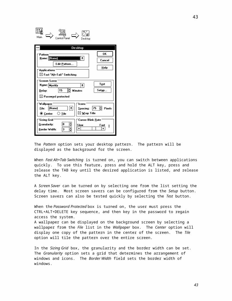
The Coordinate Readout settings box is divided into two sections. The Coordinates section contains option menus for setting the format and accuracy of coordinates and distances. The Format option menu allows you specify that coordinates and distances are displayed with Master Units (MU only), Sub Units (MU:SU), or Working Units (MU:SU:PU). From the Accuracy option menu, you can choose the number of decimal places (1-4) or the denominator of the fraction (2-64) used to display fractions of the units chosen from the Format option menu.
The Angles section contains option menus for setting the format, mode, and accuracy of angle readout. The Format option menu allows you to specify either DD.DDDD for decimal angle readout, or DD MM SS for angle readout in degrees, minutes, and seconds. From the Mode option menu, you can chose the Conventional, Azimuth, or Bearing mode of angle readout. The Accuracy option menu allows you to specify the number of decimal places (0-4) used to display fractional angle measurements.Coordinate readout formats are saved with the design file when you use the Save Settings item from the File pull-down menu.
To access the Coordinate Readout settings box click Settings>Coordinate Readout from the Microstation Command window.
Global Origin
The design plane has imaginary X and Y axes. The point at which these axes cross is the center of the design plane. Every identifiable point on the design plane has an X and a Y coordinate. That is, every point can be identified by its position on the X axes and Y axes.
The center of the design plane has the 0,0 coordinate, and this point is called the global origin. Half the values on the plane will be positive and the other half negative. However, the global origin may be moved from the center of the design plane. In mapping applications utilizing the State Plane Coordinate system the global origin can be moved to the lower left-hand corner of the design plan. This will result in all positive values. The sequence to move the global origin to the lower left corner of the design plane is keyin go=0,0, then a reset on the mouse.
43
43
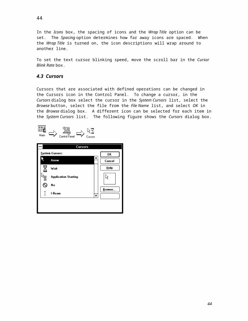
5.5 Saving and Exiting a Map File
There are several different ways that you can choose to terminate a design session. These exit methods vary depending on the amount of information you want to save. A basic workflow for exiting a file is conveyed below:
1. Compress the design file.2. Save the settings.3. Exit the design file and/or MicroStation.
Each of the above mentioned commands will be discussed in the following sections.
Compress Design
When elements are deleted from the design file, MicroStation only marks the elements for deletion. Until the design file is compressed, the elements, even though they do not display, remain in the file. When the Compress Design command is invoked, all elements marked for deletion are actually erased from the file on the disk, thus freeing storage space. This command also clears the undo buffer so nothing can be undone or redone after a compress has been performed.
To execute the command select the Compress Design item from the File pull-down menu. The message Compress in progress will be displayed indicating that the command is executing. The message File Compressed will display when it has completed.
Saving Settings
Any operation that you perform on a design element is automatically saved. However, changes that you make to your design settings are not automatically saved. Save Settings causes Microstation to remember the active symbology, view attributes, and active element settings.
To save the current design settings select the Save Settings item from the File pull-down menu. The message Settings Saved will display when the operation is complete. File Backup
One option to save a duplicate copy of your file is to issue the Backup command. If you type in backup in the input field of the Command Window and press the <Return> key, your current design file will be
44
44
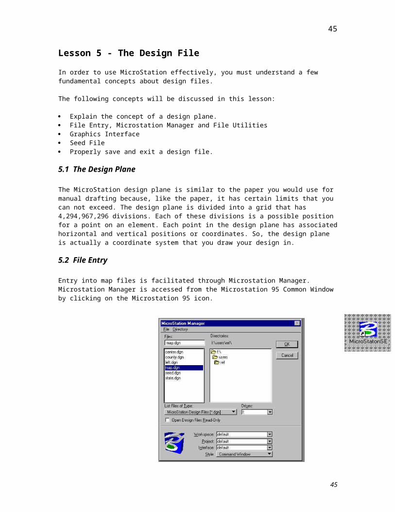
copied to a file that has the same name, but a .bak extension. The message that displays in the Command Window when the operation is complete shows you the name of the backup file. Since this command automatically copies to a set filename, future executions of this command will overwrite any existing backup file. Remember, backing up a file to the same directory on the same disk will not save you if something happens to your disk drive. Files need to be backed up to an external device such as a tape drive.
Save Design As Dialog Box
If you want to save a copy of your design file, and specify the name of the file to save it as, you will want to use the Save Design As dialog box. This dialog box is displayed by activating the File pull-down menu and selecting the Save as item. You can type in a filename in the Name data entry box or select an existing file using the Files, Directories, Filter, and Type objects. If you select an existing file, this file will be overwritten with this operation.
Exiting A Design File
To exit your design file, you can select either the Exit or Close item from the File pull-down menu. The Exit item will exit your design file and return you to the Windows environment. The Close item will close your design file and return you to the MicroStation Manager interface.
There may also be times when you want to close the current design file and open another one, without exiting MicroStation. There are two ways that you can do this. If the desired design file is one of the last four files that you attempted to enter, the name of that file will display as a numbered item on the File pull-down menu. You can display this file by tapping the data button on the menu item. This operation will automatically close the current design file before entering the chosen file.
The other way is to select the Open item from the File pull-down menu. This item will display the MicroStation Manager dialog box. From this dialog box, you can select the file that you wish to enter. Once again, the current design file will automatically be closed before the new design file is displayed.
You can also close the current design file and create a new one without ever exiting MicroStation. This is done by selecting the New item from the File pull-down menu. This item will display the same Create Design dialog box that is displayed through the MicroStation Manager interface.
45
45
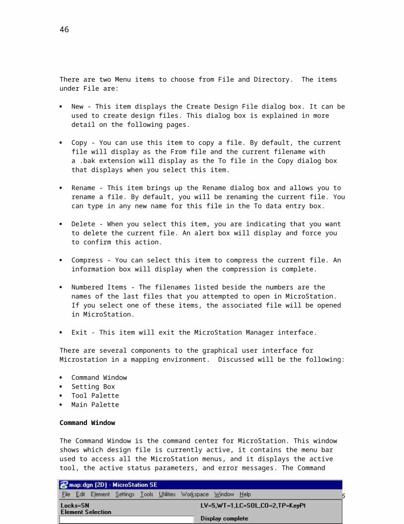
Introduction to MicroStation
Lesson 6 - Digitizing and Drawing Concepts
This lesson will discuss the types of digitizing and drawing concepts that are commonly used to perform map data capture.
6.1 Digitizing
Digitizing is the method of tracing a drawing or photograph. There are two basic type of digitizing; board and heads-up digitizing. Board digitizing involves securing a drawing on an input system, and using several of the map feature/element commands to generate vector elements in the map file to represent the features on the drawing. Heads-up involves placing map features over a scanned raster image that has been warped to control points in a map file representing real phenomenon on the surface of the earth. The raster file is warped by application software that is integrated with Microstation.
The procedure for board digitizing setup is conveyed below:
1. Create a design file.2. Set working units that are appropriate for the image being digitized, while ensuring that the design
plane working area is greater than the actual size of the image.3. Set up appropriate views. It is recommended that you set up one of the views to encompass the entire
drawing.4. Partition the digitizing tablet surface. The procedure to do this is covered later in this lesson.5. Mount the hard copy to be digitized on the tablet surface. Make sure that the features you want to map
are in the digitizing partition and not the screen partition.6. Place monument points that associate known points (of your choosing) on the hard copy with points in
the design plane.7. Activate the File pull-down menu and select the Save Settings item. This will save the working units,
view configuration, and the relationships specified by monument points, digitizer partitioning, and setup.
Partitioning divides the surface of the digitizing tablet into two areas or partitions. One area, the screen partition, continues to provide standard tablet-to-screen mapping. Within the screen partition, moving the tablet cursor results in a corresponding movement of the screen cursor, regardless of what is displayed on the screen. The other area is the digitizing partition. Within the digitizing partition, movement of the tablet cursor results in a corresponding movement of the screen pointer only within the part of the design plane to which you are mapping features of the hard copy.
The procedure for partitioning the digitizing surface is presented below:
1. From the Workspace pull-down menu, select the Digitizing item to open the Digitizing settings box.2. From the Digitizing settings box, activate the Tablet pull-down menu and select the Partition item.
3. Identify the lower left corner of the screen partition by placing the tablet cursor over it and pressing the data button.
46
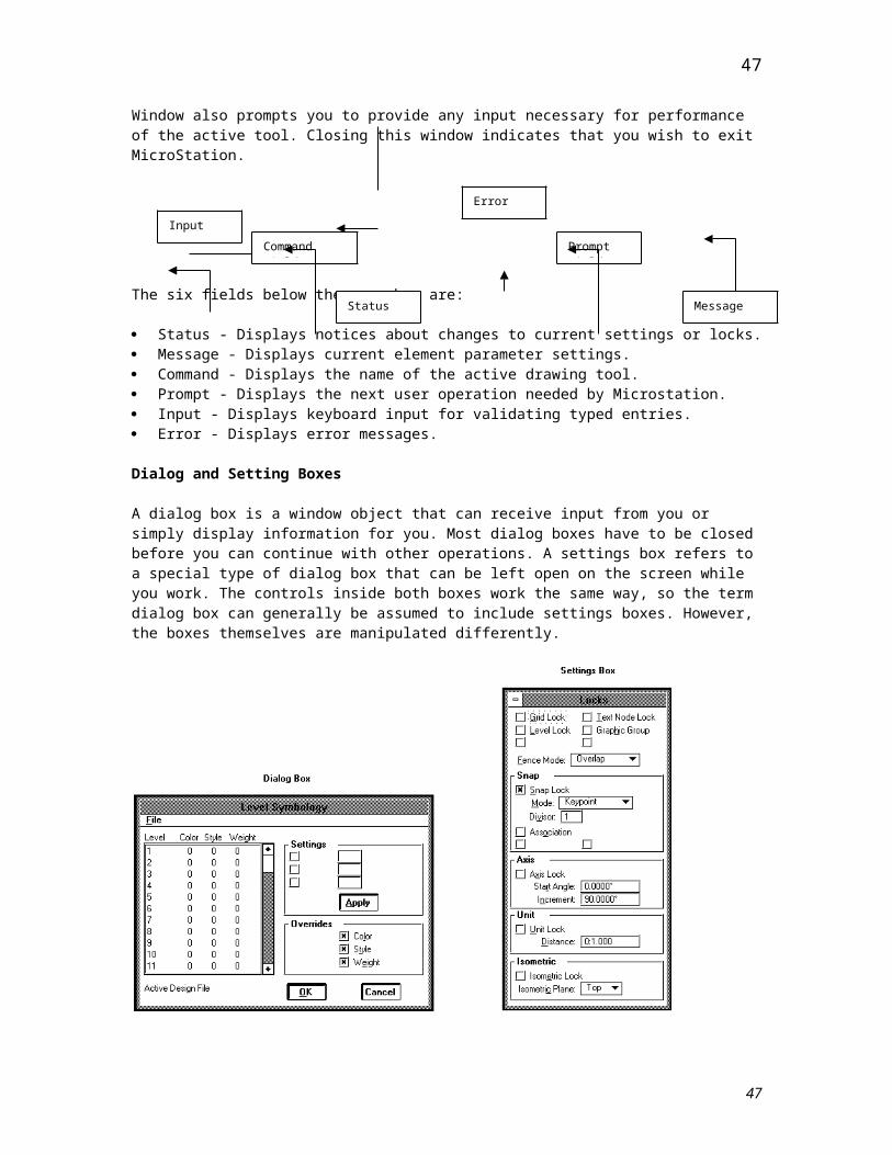
Introduction to MicroStation
4. Identify the upper right corner in the same fashion.
The screen partition takes priority over the digitizing partition. If data points are entered in the screen partition, their position in the design plane reflects their position on the screen. Therefore, make sure not to stray into the screen partition while digitizing.
The procedure to register the drawing is conveyed below:
A monument point can be any point at which the coordinate on the hard copy being digitized is known. It is advisable to define several widely spaced monument points. Monument points can be placed in the design plane as a point element using precision input.
1. (Optional) Place point elements for reference with line weights of at least 3 using the Place Active Point tool.
2. From the Settings pull-down menu, select the Digitizing item to open the Digitizing settings box.3. From the Digitizing settings box, activate the Tablet pull-down menu and select the Setup item.
4. Choose a monument point on the hard copy, position the tablet cursor over it and enter a data point. Ignore the location of the screen pointer, which only lets you know that the tablet cursor is over an active area of the tablet.
5. Move the tablet cursor into the screen partition and enter a data point in the design that corresponds to the monument point you selected in the previous step. Snapping to a point element, if one was placed for reference, or precision input is recommended.
6. Repeat the two previous steps for each additional monument point.7. After placing all monument points, reset. The system will display this message in the Command
Window:Avg. error=_%, Max. error=_%If the error values are less than 1%, the setup is acceptable. If otherwise, the setup should be repeated.
8. To confirm accurate placement of the monument points, move the cursor around the hard copy. If the monument points are correctly defined, the pointer displays in the design at points corresponding to the monument points.
The procedure for heads up digitizing setup is conveyed below:
1. (Optional) Place point elements for reference with line weights of at least 3 using the Place Active Point tool.
2. Load the raster image in using either IRASB or IRASC.3. Perform a warp of the image to the control points monuments.
47
Introduction to MicroStation
6.2 Graphic Elements/Map Features
Map files are composed of a linked list of graphic and control elements. The control elements contain information such as the active parameters, scaling information, and view information. The graphic elements are those that are displayed on the screen or plotted by Microstation. Whenever you are placing lines, linestrings, circles, arcs or shapes to represent map features you are adding elements to the end of the map file header.
The attributes of an element determine how that element will look. Element attributes include the element color, style, weight, and class. By default, the color, style, and weight all have a value of zero and the class is primary. This means that any elements you create will be primary, and they will be drawn in white, solid, thin lines.
There are two classes of elements that can be drawn in MicroStation. They are: Primary and Construction. Construction elements are usually used as drawing aids. For example, you might place a construction element in a particular location to snap other elements to, but you would not plot this element when the design is complete. Primary elements are actually part of the design.
To set the element class, or to draw elements in other colors, or with different line styles, or of varying thickness, you must change the active attributes. One way to do this is with the Element Attributes settings box. This settings box is displayed by activating the Element pull-down menu and selecting the Attributes item. The Element Attribute settings box will display.
48
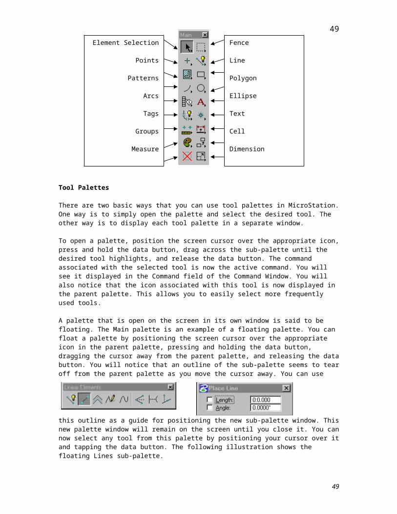
Introduction to MicroStation
6.2.1 Linear Feature Elements
There are several line element types that are used to represent linear map features. These consist of single segment and multi segment lines. Curvestrings are also utilized to depict linear map features. These element types are typically used to illustrate features such as highways, streets, trails, railroads, sewer lines, power/transmission lines, contour lines, fences, and landmark lines. These element types can be used in the construction of cells, and graphic groups. Linear measurement calculations can be performed on these elements. Linear elements can be patterned. Linear elements can be defined graphically by digitizing or with precision placement commands.
The tools on the Lines sub-palette are for placing different types of lines and line strings. As you select different tools, you should notice two things: the active command is changing in the command window and any associated settings displayed below the palette are changing. Below is the palette for placing lines.
The following sections will detail these commands.
49
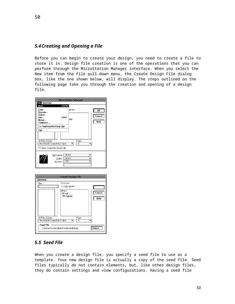
Introduction to MicroStation
6.2.1.1 Place Line
keyin: pla lin
The default Place Line tool allows you to create a line from two data points that you supply.
To place a line:
1. From the Main palette, select the Place Line tool.
2. Place a data point to define the start of the line.
3. Place a second data point to define the end of the line. Subsequent data points continue to place connected lines. Reset to finish the process, or to start a new line not connected to the previous one.
Additional parameter settings to consider when using this command are listed below:
• Length - Use this setting to specify the line length in working units.• Angle - Use this setting to indicate that the line be drawn at the specified angle. Any angle that you
specify here becomes the active angle just as if you entered it from the Active Angle settings box.
50
Introduction to MicroStation
6.2.1.2 Place Linestring
A line string is a series of adjoining line segments that are treated as one element. The maximum number of segments that can be included in one line string is 100. There are two tools on the Lines sub-palette that you can use to place line strings. They are:
NO LONGER PART LINES PALETTE, KEYIN STILL WORKSkeyin: pla lstring
Place Line String - This tool is used to a define a line string by vertices that you enter. The following settings are available with this tool:
Length - Use this data entry box to specify the length of the individual line segments that make up the line string.
Angle - Use this data entry to indicate that the line segments are to be drawn at the specified angle. Any angle entered here becomes the active angle.
Non-planar - This setting is only available in 3D design files.
keyin: pla lstring str
Place Stream Line String - This tool is used to place a stream line string. It is primarily used for tracing objects when digitizing. It allows you to define many vertices without having to enter a large number of individual data points. The movement of the tablet cursor is sampled and data points are recorded based on the following settings:
Delta - Use this data entry box to set the minimum distance, in working units, between sampled points. Tolerance - Use this data entry box to set the maximum distance, in working units, between recorded
data points. Angle - Use this data entry box to set the angle, in degrees, that when exceeded, causes the last
sampled point to be recorded as a data point. Area - Use this data entry box to set the area that, when exceeded, causes a sampled point to be
recorded as a data point.
To place a line string:
1. From the Lines sub-palette, select the Place Line String tool.2. Indicate the desired settings.3. Place a data point to define the beginning of the line string.4. Continue placing data points to define the vertices of the line string.5. Press the reset button to terminate the line string.
51
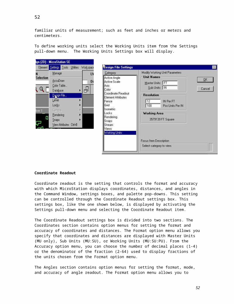
Introduction to MicroStation
In the following illustration, a line string with four vertices is created.
52
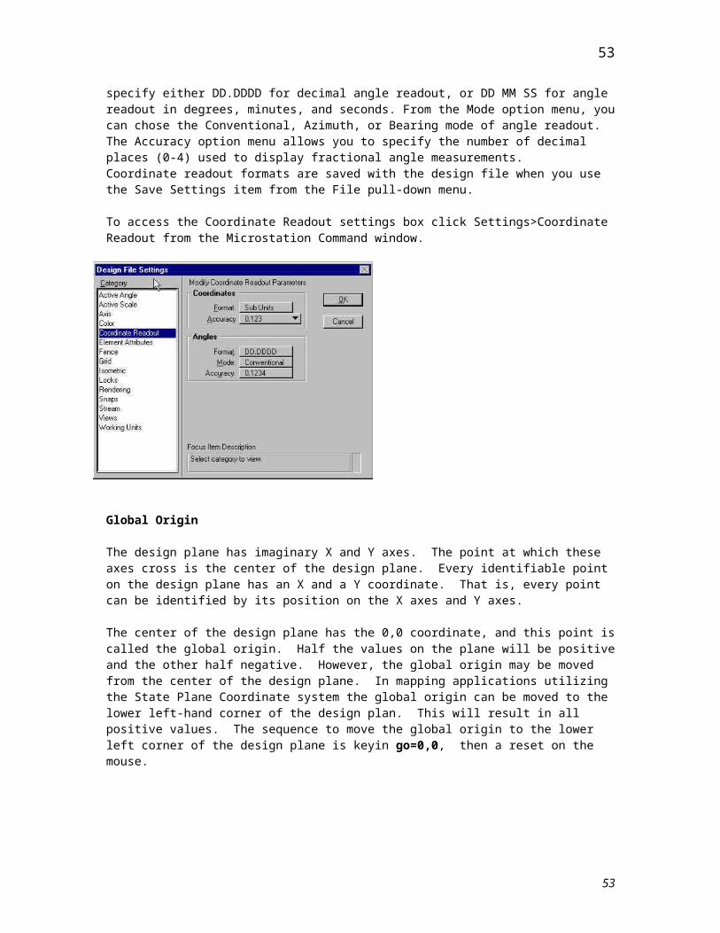
Introduction to MicroStation
6.2.1.3 Place Curvestring
This tool is used to place a point or stream curve. A point curve is placed by entering multiple data points to define the curve. To place an accurate curve, you must place data points close together on sharper bends and farther apart on smoother curves. A stream curve is used primarily for tracing images when digitizing.
The available settings for this tool are:
Method - From this option menu you can select whether the curve is a point curve or a stream curve. This is the only available setting if you choose to place a point curve in a 2D file. If you choose the Stream item, the following settings are also available.
Delta - Use this data entry box to set the minimum distance, in working units, between sampled points. Tolerance - Use this data entry box to set the maximum distance, in working units, between recorded
data points. Angle - Use this data entry box to set the angle, in degrees, that when exceeded, causes the last
sampled point to be recorded as a data point. Area - Use this data entry box to set the area that, when exceeded, causes a sampled point to be
recorded as a data point.
NOTE: A curve element can have from 3 to 97 vertices. If more than 97 vertices are defined, a complex chain consisting of one or more curve elements is created.
To place a point curve:
1. From the Linear Element tool palette, select the Place Points or Stream Curve tool.2. From the Method option menu, choose the Stream item.3. Enter a data point to define the beginning of the curve.4. Continue to enter data points to define the curve. You must enter at least three points to define a
normal curve. Reset when the curve is complete.
53
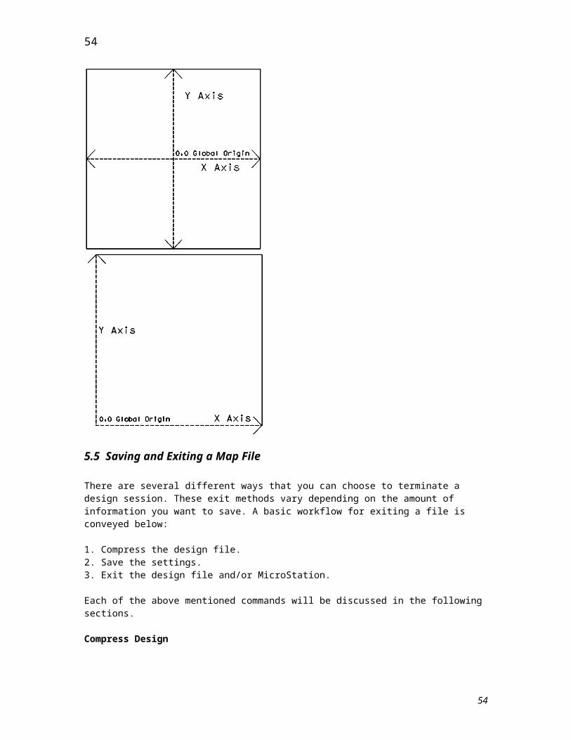
Introduction to MicroStation
In the following illustration, 5 data points are used to define a point curve.
54
Introduction to MicroStation
6.2.2 Area Feature Element Types
Polygons/shapes are typically used to represent area features and planimetric data on topographic maps and site plans. One of the most common usages of polygons is to represent building pads. The Place Block commands facilitate the definition of simple building pad data. More complex building pads can be created by using multisided or orthogonal shapes. Multisided shapes are also used to layout closed traverses, political boundaries, lakes, voting districts, and general land use patterns. Area calculations, hatching, cross-hatching, and area patterning can be performed on shapes. Active element attributes will impact the appearance of these feature types when placed in map files. Polygon feature types can be defined graphically with the mouse or by precision input. Polygons can be component part of cells.
Below is the Polygon palette.
The following sections will profile the specific polygon commands.
55
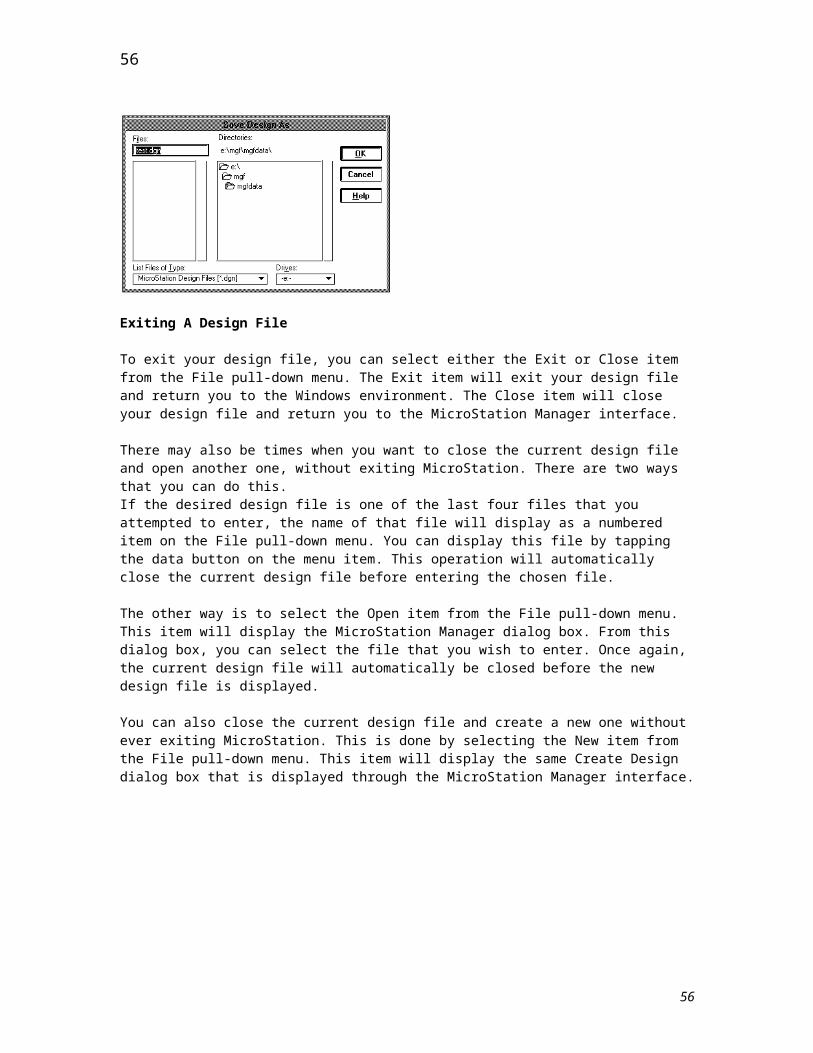
Introduction to MicroStation
6.2.2.1 Place Block
keyin: pla blo
The settings for the Place Block tool allow you to define the placement method, area, fill type, and fill color you want for your block. The available settings are:
Method - This setting determines how the block is oriented. The two choices on this option menu are:
Orthogonal - The block is orthogonal to the view in which the first data point is entered.Rotated - The block's orientation is defined with a data point.
Area - From this option menu, you can establish whether the block is a Solid or Hole. A solid contains the area in which it is placed and it can be patterned. A hole is without area and it cannot be patterned. A hole will actually eliminate area when it is placed within a solid element.
Fill Type - The items on this option menu determine how or if the block is filled. The available items are:
None - The block will not be filled.Opaque - The block will be filled with the active color.Outlined - The block will be filled with the active fill color and outlined with the active
color.
Fill Color - You can enter the desired fill color number in this data entry box, or select it from the associated color palette. If the Fill Type is Outlined, this color can be different from the active color.
NOTE: Fill is a view attribute that can be toggled on or off through the View Attributes settings box. By default, fill is off in all views.
To place a block:
1. From the Polygons tool palette, select the Place Block tool.2. Choose the desired placement method, area, fill type, and fill color from the tool settings area.3. Enter a data point to define one corner of the block.4. If the Method is Orthogonal, enter a second data point to define to diagonal of the block.
56
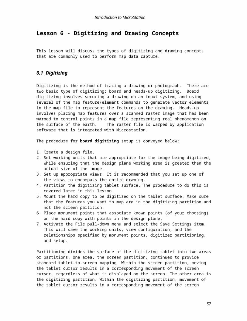
Introduction to MicroStation
In the following illustration, a solid, unfilled, orthogonal block is created.
If the Method is Rotated, enter a second data point to define the orientation of the block's base, and a third data point at the corner diagonally opposite the first data point.
57
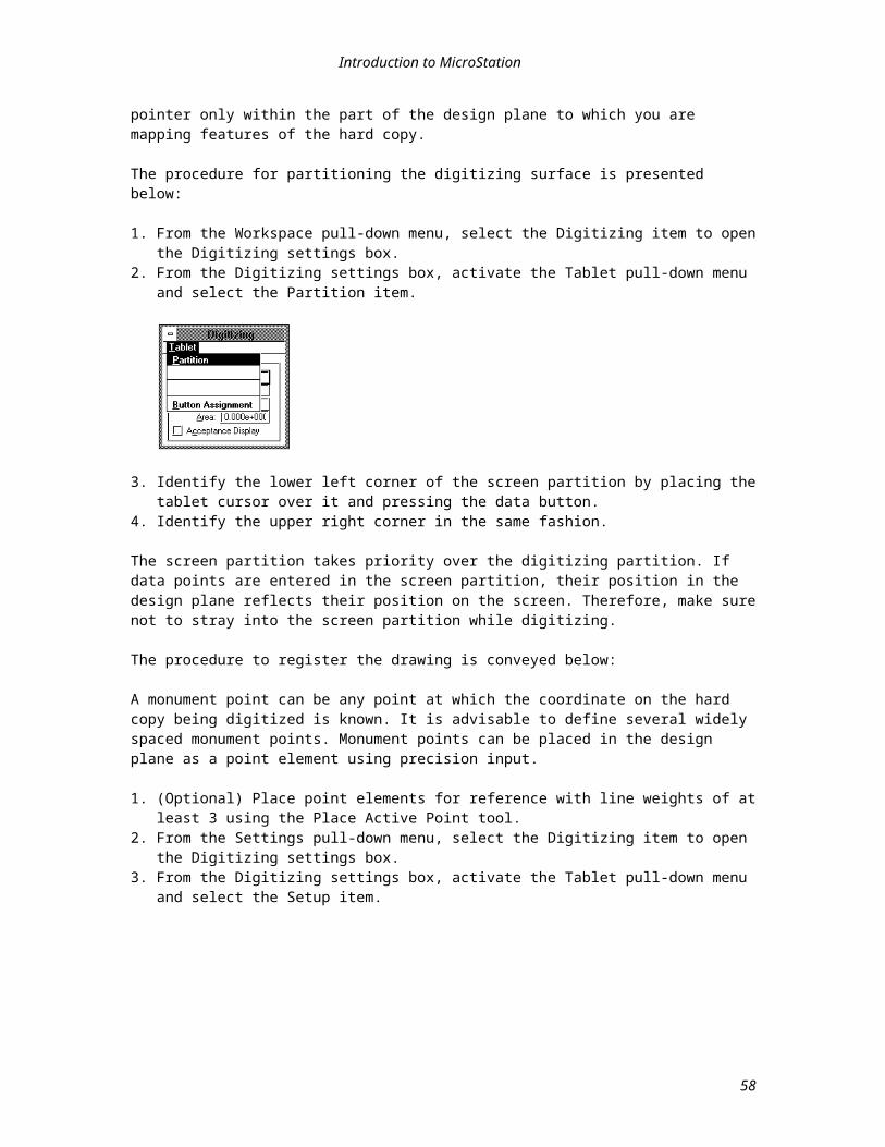
Introduction to MicroStation
6.2.2.2 Place Shape
keyin: pla sha
This command will allow the placement of a multi-sided shape of between 4 and 100 vertices.
To place a multi-sided:
1. From the Polygons tool palette, select the Place Shape tool.2. Choose the desired settings (area, fill type, and fill color) from the tool settings area.3. Enter a series of data points to define the shape.4. Place the last data point on top of the first to close the shape or choose the Close Element button.
In the following illustration, a solid, unfilled, multi-sided shape is created.
58
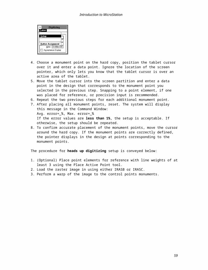
Introduction to MicroStation
6.2.2.3 Place Orthogonal Shape
keyin: pla sha ort
This tool is similar to the Place Shape tool. It too lets you create a shape that has from 3 to 100 vertices. The difference is that all the angles in this shape are forced to 90 degrees. You also close this shape by placing a data point in the same location as the original data point.
To place an orthogonal shape:
1. From the Polygons tool palette, select the Place Orthogonal Shape tool.2. Choose the desired settings (area, fill type, and fill color) from the tool settings area.3. Enter a series of data points to define the shape.4. Place the last data point on top of the first to close the shape.
In the following illustration, a solid, unfilled, orthogonal shape is created.
59
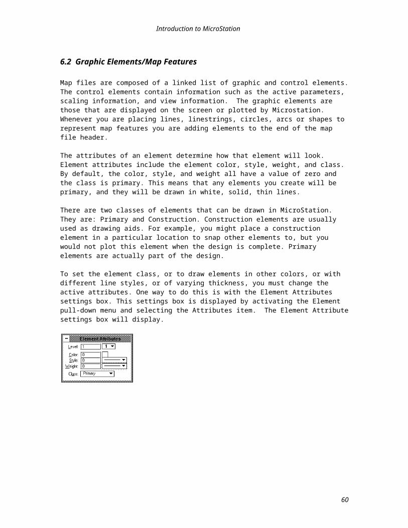
Introduction to MicroStation
6.2.3 Point Feature Element Types
Several different commands are available to generate point feature types.
Circles are common elements that are used for this purpose. Circles are used to represent tanks (oil and water), landmarks, wells, fire hydrants, utility poles, and highway signing. These element types will assume the default element attribute settings when placed in a map file. Circle element types can be patterned, hatched, and cross hatched. Area calculations can also be performed on circles. Circles can also be component parts of cells. Circles can be defined graphically or with precise input values.
Another element type that can be used to represent a point feature is a point element. A point element is a zero-length line. This element type will assume the default element attribute settings when placed in a map file.
These element types will be described in the following sections.
60
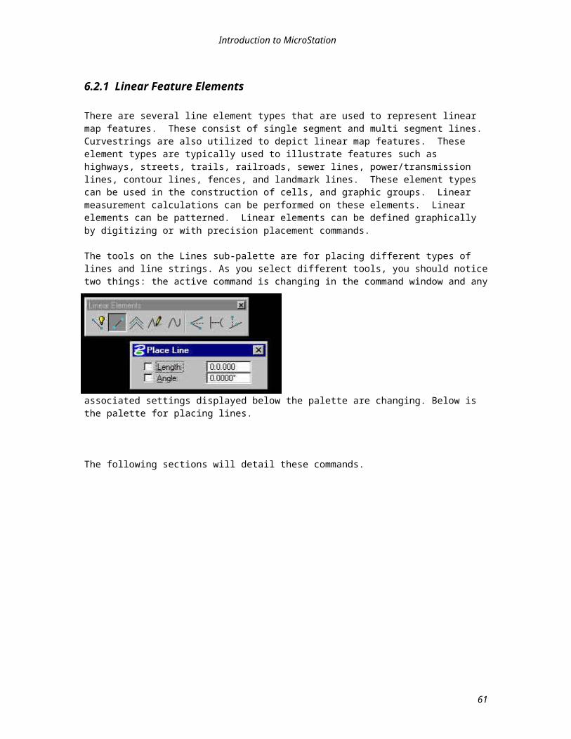
Introduction to MicroStation
6.2.3.1 Place Circle by Center
keyin: pla cir cen
This tool allows you to place a circle by indicating its center point and a point that lies somewhere on it. This second point can either be defined graphically, or by specifying a desired radius. The available settings for the Place Circle by Center tool are:
Diameter - Use this check button/box and its associated data entry box to indicate the circle's diameter value.
Area - Use this option menu to indicate whether the circle is a solid or hole.
Fill Type - Use this option menu to set the desired fill type.
Fill Color - Use this data entry box, or the associated color palette, to set the desired fill color.
To place a circle:
1. From the Ellipses tool palette, select the Place Circle by Center tool.2. Select any desired settings from the tool settings area.3. Enter a data point to define the center of the circle. If the Diameter check button/box is selected, the
circle will be drawn using the center point, and diameter/radius you supplied.4. If Diameter is not selected, enter a second data point to define a point on the circle.
61
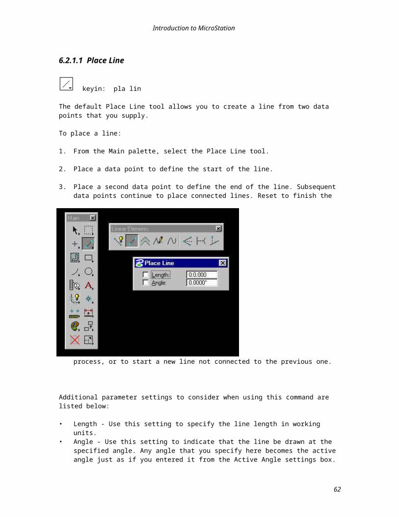
Introduction to MicroStation
The following illustration shows the placement of a solid, unfilled circle with a specified radius of 5 master units (ft).
62
Introduction to MicroStation
6.2.3.2 Place Circle by Edge
keyin: pla cir edg
This command allows to create a circle by supplying three data points that lie on the edge of the desired circle.
To place a circle:
1. From the Ellipses tool palette, select the Place Circle by Edge tool.2. Select any desired settings from the tool settings area.3. Enter a data point to define the beginning point of the circle.4. Enter a data point to define the second point of the circle5. Enter a third data point to complete the definition of the circle.
Below is an illustration.
63

Introduction to MicroStation
6.2.3.3 Place Circle by Diameter
keyin: pla cir dia
The Place Circle by Diameter tool allows you to create a circle by inputting two data points to define the diameter of the circle.
To place a circle:
1. From the Circles & Ellipses tool palette, select the Place Circle by Diameter tool.2. Select any desired settings from the tool settings area.3. Enter the first point to define the diameter of the circle.4. Enter a second point to complete the definition of the diameter of the circle.
Below is an illustration.
64
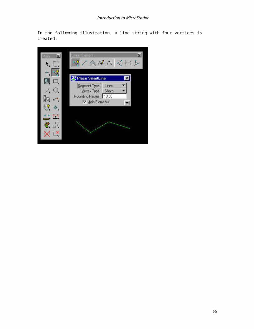
Introduction to MicroStation
6.2.3.4 Place Active Point
keyin: pla poi
Active points are used to mark a specific location in a design file. These points, which may be in space or on an element, can be manipulated like any other element. One of the best features of active points are the various tools that automatically calculate placement based on some established criteria. Once you have the active points placed, it is easy to go back and drop in cells, text, or other elements at the active point locations. In this lesson, you will see how to establish something as an active point and how to position it in your design file.
There are certain objects that appear in the tool settings portion of the Points palette no matter which tool is currently active. They are:
Point Type - From this option menu you can choose the type of active point you want to place. The choices that you have are:
Element - If you select this choice, your active point will be a point element, which is actually a zero length line. Since it is an element, all the active element attributes will still apply. You will probably want to increase the weight attribute so that the point will be visible on the screen.
Character - This choice allows you to specify a single character to be used as the active point. The active font, text height, text width, and the active angle will determine how the character is placed.
Cell - This choice allows you to use a cell from the attached cell library as the active point. The active angle and active scale will determine how the cell is placed.
Character - If the Point Type is set to Character, the character entered in this data entry box will be the active point.
Cell - If the Point Type is set to Cell, the cell entered in this data entry box will be the active point. You can also set the cell to use as the active point through the Cell Library settings box.
To place the active point:
1. From the Points palette, select the Place Active Point tool.2. Enter the appropriate information in the settings objects to set the desired active point.3. Enter a data point or use precision placement to place the active point. Subsequent data points will
continue to place the same active point.The following illustration shows the placement of the active point.
65
Introduction to MicroStation
66
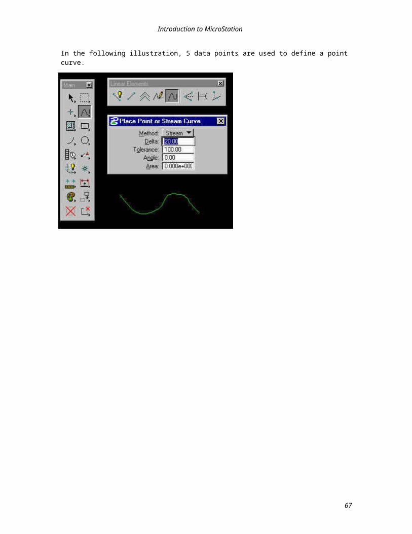
Introduction to MicroStation
6.2.4 Arcs
Arcs are open elements that can be used to generate linear element types. Common applications for arcs are roads and highways. They can be used to construct cul-de-sacs and curbs for roads. In highway applications, arcs are used to represent on/off rams and access roads. Arcs can also be a composite part of a complex element (individual elements with common endpoints that are chained together into one element). Arcs will take on the active element attribute settings upon placement.
The following sections will describe the most commonly used arc commands in digital mapping applications.
67
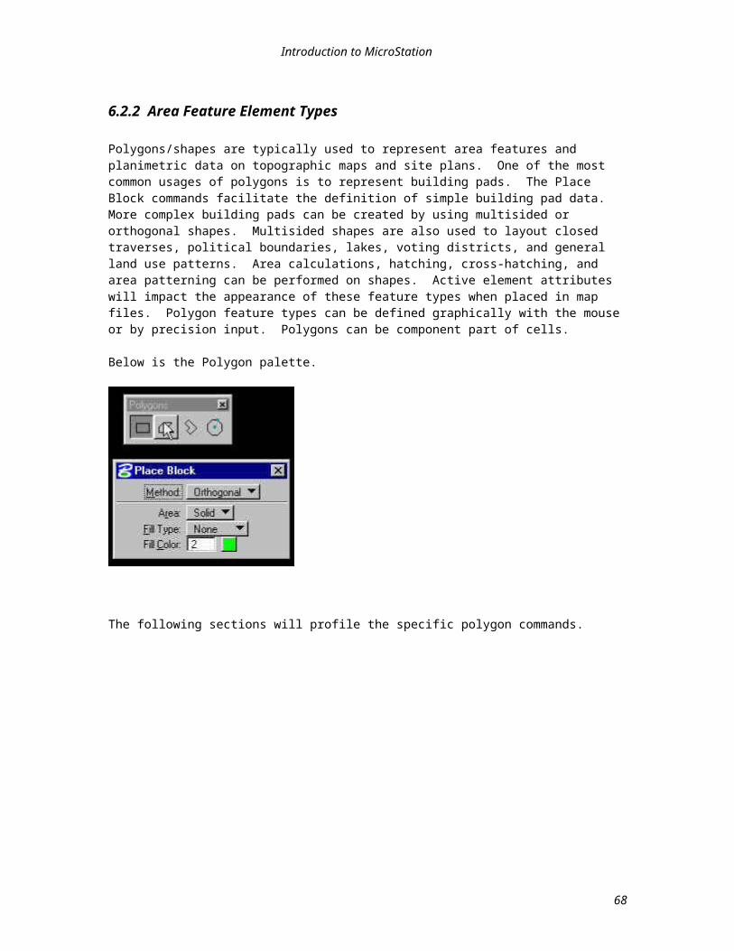
Introduction to MicroStation
6.2.4.1 Place Arc by Center
keyin: pla arc cen
This tool is used to create a circular arc that is defined by an endpoint, center, and sweep angle. The available settings for this tool are:
Radius - If this check button/box is on, the value in the associated data entry box is used as the arc's radius.
Start Angle - If this check button/box is on, the value in the associated data entry box sets the angle between an imaginary line between the center and the arc's beginning and the view's x-axis.
Sweep Angle - If this check button/box is on, the value in the associated data entry box sets the sweep angle.
To place an arc by center:
1. From the Arcs tool palette, select the Place Arc by Center tool.2. Enter a data point. If Radius, Start Angle, and Sweep Angle are all on, this data point defines the
center and places the arc. With any other combination of constraints, this data point defines the arc's beginning.
3. If necessary, enter a second data point to define the arc's center.4. If necessary, enter a third data point to define the arc's endpoint.
68
Introduction to MicroStation
The following illustration shows the placement of an arc using three graphically defined points.
69

Introduction to MicroStation
6.2.4.2 Place Arc by Edge
keyin: pla arc edg
This tool also uses three data points to create an arc. The difference is that this time the three points are all points that lie along the edge of the desired arc. The first point is the beginning of the arc, the second point is a point on the arc's edge and it also indicates the desired direction, and the third point is the arc's endpoint.
Radius - If this check button/box is on, the value in the associated data entry box is used as the arc's radius.
Start Angle - If this check button/box is on, the value in the associated data entry box sets the start angle.
Sweep Angle - If this check button/box is on, the value in the associated data entry box sets the sweep angle.
To place an arc by edge:
1. From the Arcs tool palette, select the Place Arc by Edge tool.2. Enter a data point to define the arc's beginning. If Radius, Start Angle, and Sweep Angle are all on, the
arc is placed.3. If necessary, enter a second data point to define a point on the arc.4. If necessary, enter a third data point to define the arc's endpoint and sweep angle.
In the following illustration, an arc is placed by three graphically defined points along the arc's edge.
70
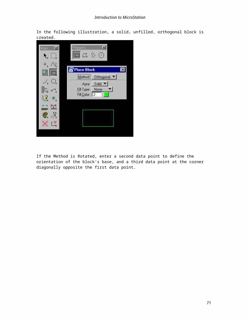
Introduction to MicroStation
6.2.4.3 Arc Modification Commands
Modify Arc Radius - You can modify the radius, sweep angle, and center of a circular arc with this tool. The endpoints will not move.
Modify Arc Angle - This tool is used to extend or shorten the length of an arc.
Modify Arc Axis - You can use this tool to lengthen or shorten an arc's axis.
71
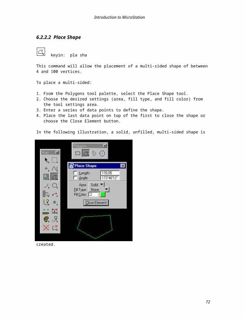
Lesson 7 - Levels and View Manipulations
In this lesson you will learn to manipulate both level and views.
One of the nicest features about Microstation’s level setup is that each of the 63 levels can be turned on or off independently. Another nice feature is that each of the eight design views can be set up to display a different combination of levels.
Each view can be individually toggled on or off. There are several ways that you can do this. The simplest way to turn off a view is to use the Control menu to close the view. You can select the Close item from the control menu or double tap the data button on the icon. Either action will close the view.
Another way to open or close views is to activate the View pull-down menu and select the Open/Close item. This item has a sub-menu associated with it, so you will need to slide your cursor to the right to display it. Once the sub-menu is displayed, you can choose the view number item for the view you wish to turn on or off.
72
72
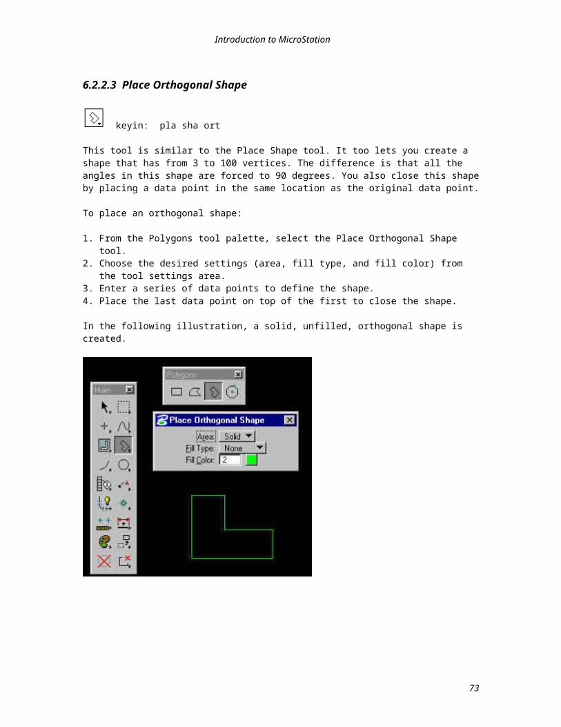
7.1 Levels
The level commands can be accessed by either keyin or the View Levels setting box.
Even though there are 63 levels that you can draw on, only one level is considered active at any given time. Any elements that you create will be placed in the active level. The View Levels settings box can be used to set the active level and to turn levels on and off in the individual views.
73
73
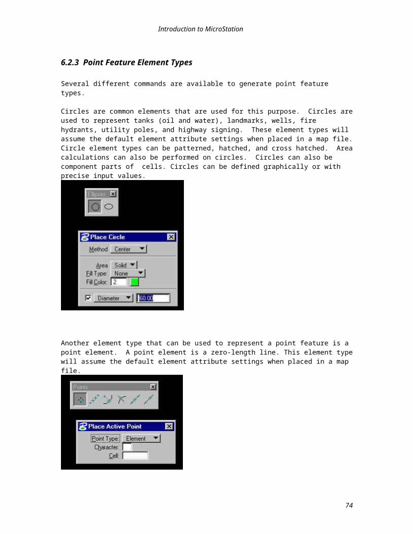
7.1.1 Active Level
Even though there are 63 levels that you can draw on, only one level is considered active at any given time. Any elements that you create will be placed in the active level. The View Levels settings box can be used to set the active level and to turn levels on and off in the individual views.
You can display this settings box by activating the View pull-down menu and selecting the Levels item. The following illustration shows the default level settings. The circle that displays around level 1 indicates that it is currently the active level. The darkened boxes around all the other levels indicate that they are turned on for this particular view. The active level is also displayed, with its associated LV= key-in, in the Message field of the Command Window.
NOTE: Changing the active level only affects elements that are created from that point on. It does not effect any existing elements.
To set the active level:
1. From the View pull-down menu, select the Levels item to display the View Levels settings box.2. In the settings box, position the screen cursor on the number for the level you want to make active, and
double tap the data button. The view number is highlighted with a circle.3. Select the Apply button.
keyin: lv= (the level number)
74
74

7.1.2 Levels On/Off
To turn levels on or off:
1. From the View pull-down menu, select the Levels item to display the View Levels settings box.2. Enter the desired view in the View data entry box.3. Position the screen cursor on the number for the level you want to turn on or off, and tap the data
button. This will toggle the level off if it was on or on if it was off. You can also press and hold the data button and drag across several numbers to turn multiple levels on or off.
4. Select the Apply button to apply the level display to the indicated view, or the All button to apply it to all views.
The following View Levels settings box indicates that levels 1 - 25 are on in view 1, and that level 25 is the current active.
keyins: on= (level numbers) of= (level numbers)
75
75
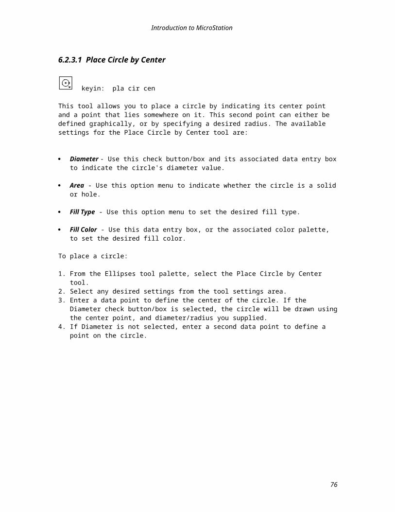
7.1.3 Change Level
keyin: chan lev
The settings for the Change Element Attributes tool allow you to specify which element attributes you want to change and the new value that you want them to have. The attributes you can change through this tool are:
Level Color Style Weight Class
To change an element's level:
1. From the Change Element palette, select the Change Element Attributes tool.2. In the tool's settings box, tap the data button in the check button/box beside the level attribute.3. Enter the new level in the field associated with the attribute. Note: This changes the drawings Active Level.4. Identify the element you wish to move to the new level with a data point.5. Tap another data point to accept the element and initiate the change.
76
76
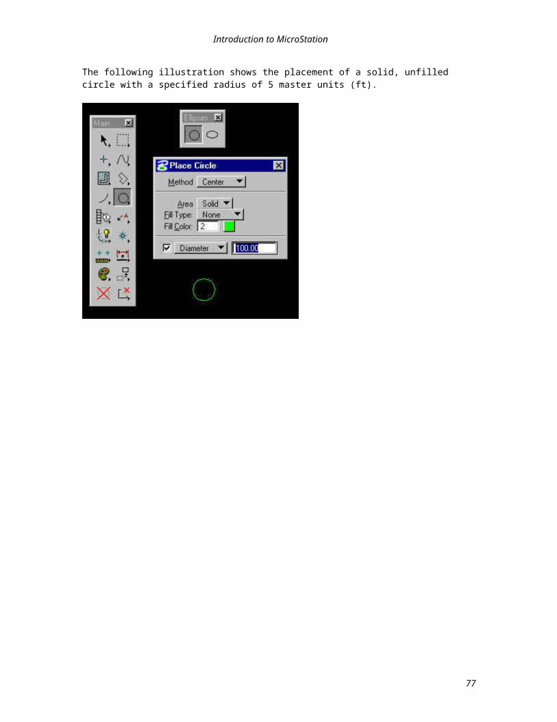
7.1.4 Level Symbology
You can define an alternate symbology for all elements on a level, making it easier to identify which elements are on a particular level. You can then display elements with their normal element symbology or with the level symbology.
To define level symbology:
1. From the Settings pull-down menu, select Level >Symbology item to open the Level Symbology dialog box.
2. In the Settings portion of the Level Symbology dialog box, select the desired color, style, and weight with the check buttons/boxes and the associated option menus.
3. In the list box, set the level or range of levels that you want to apply these attributes to.4. Select the Apply button.
NOTE: Level symbology color applies only to the outline color of closed elements.
77
77
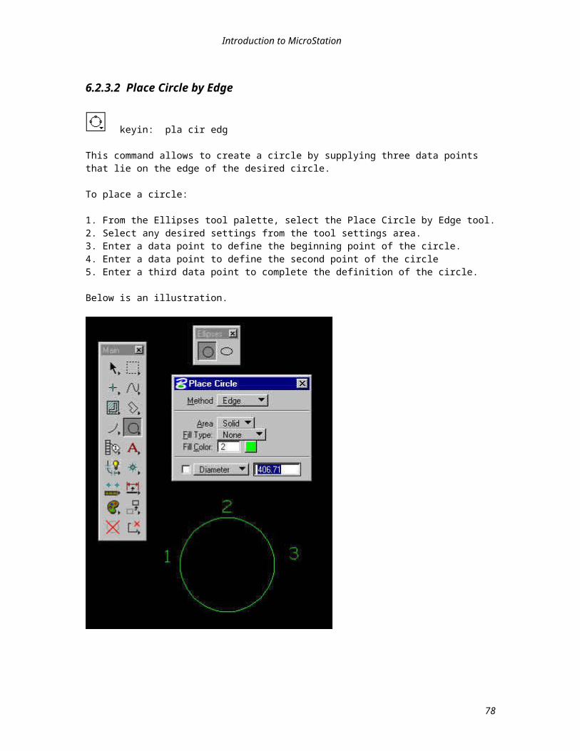
7.1.5 Displaying Level Symbology
Two conditions must be satisfied to display elements with their level symbology: both the Level Symbology view attribute, and the Level Symbology Overrides have to be on.
To display level symbology:
1. From the Settings pull-down menu, select the Level Symbology item to display the Level Symbology dialog box.
2. In the Overrides section of this dialog box, turn on the level attributes that you want to display in place of the elements' attributes.
3. Select the OK button to save the changes and dismiss the dialog box.4. From the View pull-down menu, select the View Attributes item to display the View Attributes
settings box.5. Choose the desired view from the View option menu.6. Turn on the Level Symbology attribute.7. Select the Apply button to display level symbology in the selected view, or the All button to display it
in all views.
NOTE: You may need to update the effected view(s) to see the change.
78
78
7.2 View Manipulations
The concept of views can be simplified by thinking of eight cameras available for viewing one design file. Each camera can see different areas, or all eight can be focused on the same elements. The analogy can be extended further, since many cameras permit placing filters between the subject and the lens to enhance or alter the way certain objects appear to the person viewing them. There are many MicroStation view settings that perform similar functions. Several will be described in this class to change the way your drawing appears on the screen.
The following sections will detail how views can be manipulated.
79
79
7.2.1 Displaying Views
Each view can be individually toggled on or off. There are several ways that you can do this. The simplest way to turn off a view is to use the Control menu to close the view. You can select the Close item from the control menu or double tap the data button on the icon. Either action will close the view.
Another way to open or close views is to activate the View pull-down menu and select the Open/Close item. This item has a sub-menu associated with it, so you will need to slide your cursor to the right to display it. Once the sub-menu is displayed, you can choose the view number item for the view you wish to turn on or off.
The Dialog item on Open/Close sub-menu will display the settings box shown below. This box allows you to toggle views on and off any time you want.
keyins: vi on (view number)vi of (view number)
80
80
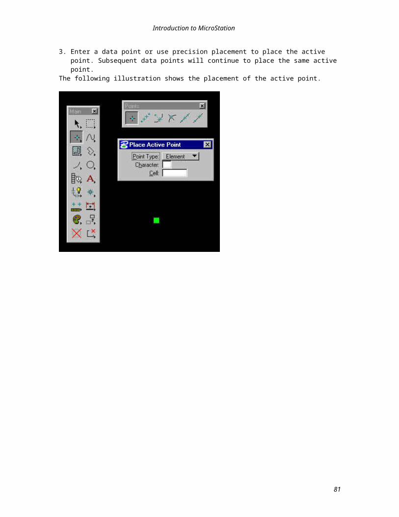
7.2.2 Window Tile
When more than one view is open, there are several default ways to arrange them on the screen. The Tile item from the View pull-down menu will identically size each view, lining them up side by side. If more than three views are open they will be placed in two rows on your screen. The following illustration shows how the Tile operation would arrange four open views.
keyin: wind ti
81
81
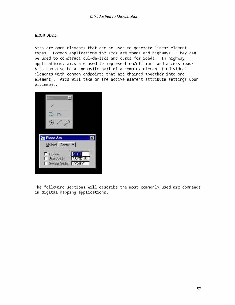
7.2.3 Window Cascade
The Cascade item from the View pull-down menu is another way to arrange all open views.
The following illustration shows four cascaded views.
keyin: wind cas
82
82
7.2.4 View Controls
The View Control palette contains controls that you can use to change the displays of views, without effecting the elements in your design file.
The following sections will discuss the view control options available.
83
83
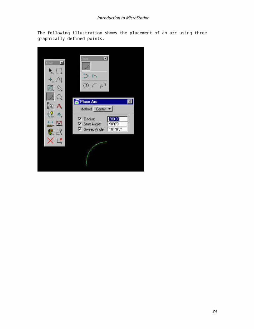
7.2.4.1 Zoom In/Zoom Out
keyin: z i
Zoom In allows you to magnify the details of the objects being viewed. When you select this tool, you will be prompted to supply the point that you want to in about. Place a data point at the center of the area you want to enlarge. Each zoom in that you perform makes the objects in the zoomed in view appear twice as large. With the keyin command you can also specify zoom scale factors. Zoom factor of 4 would make the object 4 times larger.
keyin: z o
Zoom Out allows you to decrease the magnification of the area being viewed. When you select this control, you will be prompted to supply the point that you want to zoom out about. Each zoom out that you perform makes the objects in the zoomed out view appear half the size they were before the zoom operation. With the keyin command you can also specify zoom scale factors. Zoom factor of 4 would make the object 4 times smaller.
84
84
7.2.4.2 Window Magnification and View Commands
keyin: win are
The Window Area control allows you to view an area that you define. After you select this control, you will be prompted to supply two data points. These data points define the area of your design that you wish to display. You will then be asked to select the view that you want to see this area displayed in. A data point anywhere in any open view will do.
keyin: win cen
The Window Center allows you to define a new viewing area by specifying a new center of the view. When you select this control, you will be prompted to place a data point at the location that you want to become the center of a view. Then you must select the view that you want to be centered around this point.
keyin: fit
The Fit Active Design control allows you to make every visible element in the design display in a selected view. If every element in a design has been drawn on one area of the design plane, this control works well. However, if elements have been drawn on many areas of the design plane, performing a fit may cause the elements to appear very small or as bright dots within the selected view.
keyin: updkeyin: upd all
The Update View control lets you update the contents of the selected view. Afteractivating the control, respond to the prompt, Select View, by placing a data point in any view(s) that you want to be updated. The keyin, Update All, allows you to refresh all the views that are opened.
85
85
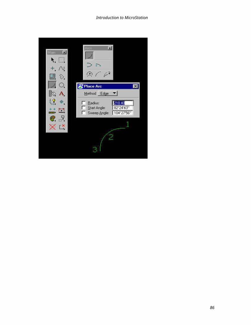
7.2.4.3 Dynamic Panning
You can also dynamically pan in a view.
To dynamically pan in a view window with the mouse:
1. Press the <Shift> key and hold it down.2. Point in the view, press the Data button, and hold it down.3. The pointer location defines the anchor point for panning. Drag away from the anchor point towards
the part of the design that you want to move into the view.
- When panning begins, you can release the <Shift> key. - To increase the speed of panning, drag the pointer further from the anchor point. To pan in a different
direction, move the pointer past the anchor point in the new direction.4. To stop panning, release the Data button.
NOTE: You can dynamically pan in a view even when a drawing tool or view control is selected.
7.2.4.4 Panning
keyin: pan
The PanView control lets you pan the selected view. After activating the control, respond to the prompt, Select View, by placing a data point in any view(s). A dynamic arrow attaches to the cursor.
The view pans in the opposite direction to the arrow.
86
86
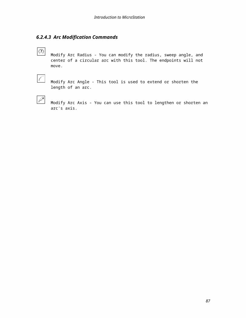
Lesson 8 - Element Manipulations, Precision Input and Snap Locks
In this lesson element manipulations, precision input of feature data, and snap locks will be discussed.
87
8.1 Element Manipulations
The tools on the Manipulate Element sub-palette facilitate editing of a drawing or the creation of more complex elements from simple elements. Below is the Element Manipulation Tool palette.
The tools that will be discussed are listed below:
Copy Move Scale Delete Undo Analyze
88
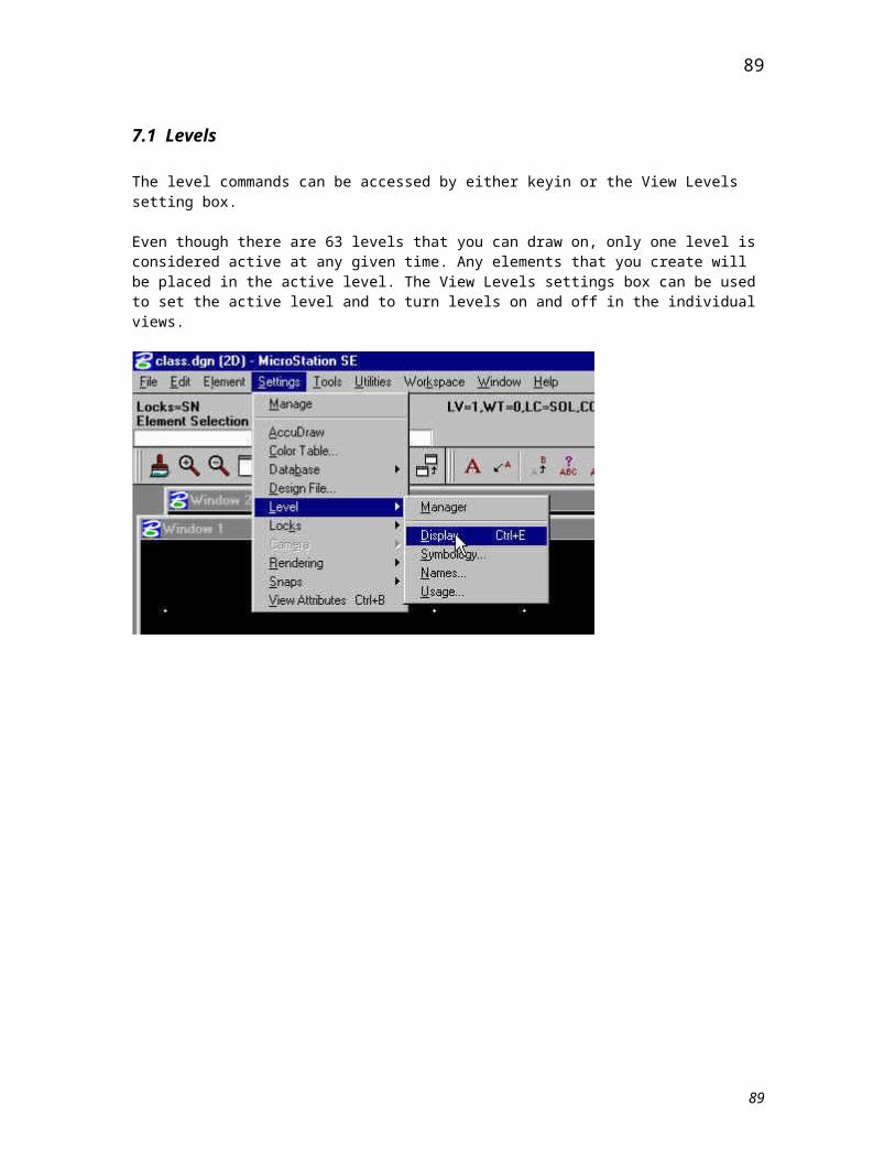
8.1.1 Copy Element
keyin: cop
The Copy Element tool allows you to duplicate any element in your design file. A fence can be used to copy multiple features simultaneously.
To copy an element:
1. Select the Copy Element tool from the Manipulate Element palette.2. Tap a data button anywhere on the element that you want to copy. The position of this data point
becomes the origin point for the placement of the new copy.3. Drag the dynamic copy of the element to the desired placement location and tap the data button to
position the copy. Additional data points will place additional copies of the element, or a reset will terminate the command.
An illustration is provided below:
89
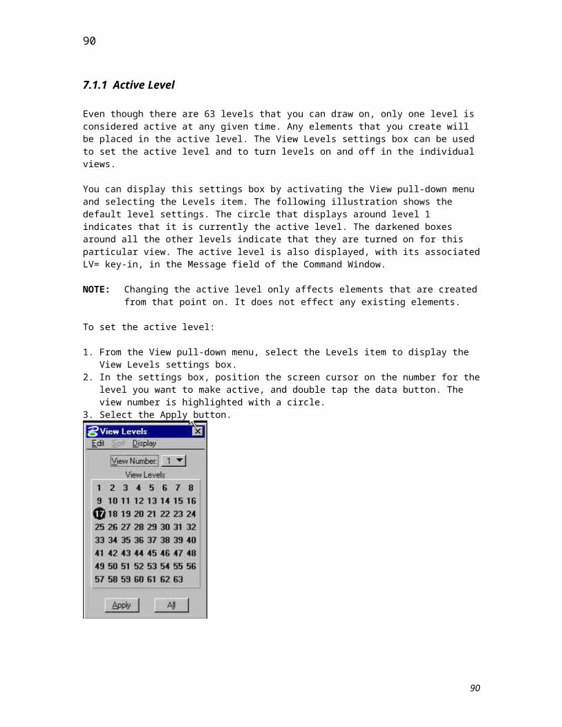
8.1.2 Move Element
keyin: mov
This tool can be used to move any element in your design file. A fence can be used to move multiple features simultaneously.
To move an element:
1. Select the Move Element tool from the Manipulate Element palette.2. Tap the data button on the element you want to move.3. Drag the dynamic element to the desired location and tap the data button to position the element.
Additional data points will continue to move the element.
90

8.1.3 Scale Element
keyin: sca
This tool allows you to resize an element by the active scale factor. With the associated settings, you can set the active scaling factor and choose whether to scale the original element or a copy. The lock icon that appears beside the scale data entry boxes determines if the element can be disproportionately scaled.
To proportionately scale an element:
1. Select the Scale tool from the Manipulate Element palette.2. Enter the desired scale factor in either the X Scale or Y Scale data entry boxes.3. Tap the data button on the element you want to scale.4. Drag the dynamic element to the desired location and tap another data button to accept the element at
its new size and position. This data point is the point about which the element is scaled. Additional data points will continue to scale the element.
91
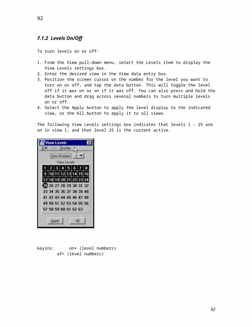
To disproportionately scale a copy of an element:
1. Select the Scale tool from the Manipulate Element palette.2. Tap on the lock icon to unlock it.3. Enter the desired scale factor in the X Scale and/or Y Scale data entry boxes.4. Select the Make Copy check button/box.5. Tap the data button on the element you want to scale.6. Drag the dynamic scaled copy to the desired location and enter a data point to accept the new size and
position. Additional data points will place additional copies, each time scaling by the scale factor.
92
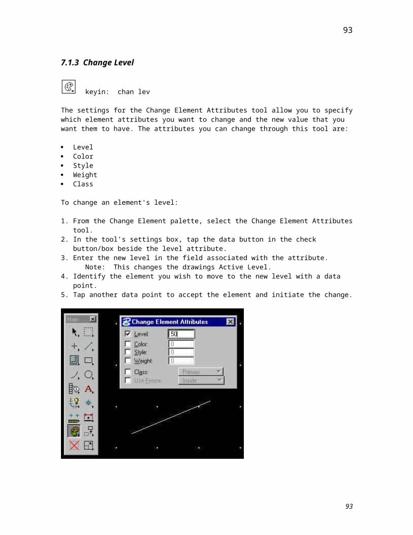
8.1.4 Delete Element
keyin: del
The Delete tool is used to erase elements from your screen. These erased elements can be recovered as long as your design file has not been compressed. Since the deletion of elements is a serious action, you will always be prompted to confirm the deletion before it takes place.
When you are prompted, in the Command Window, to confirm the delete action, you can press the data button to accept the action and delete the highlighted element, or press the reset button to reject the action. With the Delete tool, as well as other MicroStation manipulation tools, if you reject the action and there is another element very close to the position where the original element was identified, that element will be selected for the manipulation. If there are more than two elements clustered together at this location, each time the reset button is pressed a different element will highlight in the order they were placed in the design file. When the correct element highlights, you can press the data button to accept the action for this element.
To delete an element:
1. From the Main palette, select the Delete tool.2. Identify the element to be deleted by placing a data point anywhere on the element. The element will
highlight.3. Accept the element to be deleted with a data point. The element is erased from the screen. If this data
point is on another element, that element will be identified for deletion, and must be accepted or rejected.
93
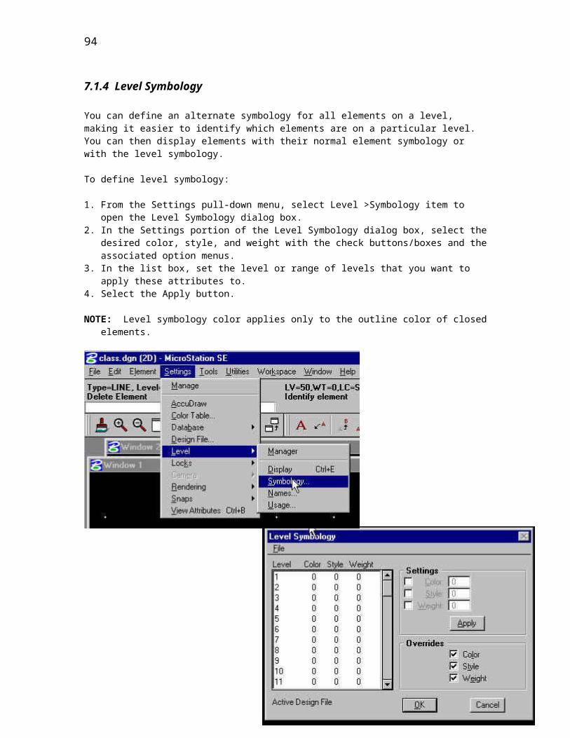
8.1.5 Undo and Redo Operations
Within certain limits, MicroStation allows you to undo and redo operations to recover from mistakes. One limit on the undo operation is the size of the undo buffer. This buffer is an area of memory that MicroStation sets aside for recording drawing operations. The smaller this buffer is, the fewer operations that can be negated. The default size for the undo buffer is 256 KB. The Undo Buffer is set in User Preferences>Memory Usage. A second limitation on undoing is that you cannot undo operations made before the design file was last closed or compressed. When you close or compress a design file, the undo buffer is automatically emptied.
The Edit pull-down menu has items that you can use to access the information in your undo buffer. The following illustration shows this pull-down menu and one of its associated sub-menus. The applicable menu items are discussed of the following page.
The Undo Item keyin: undo
The Undo item negates the last drawing operation that you performed. When you select the Edit menu, the Undo item will automatically have the name of the last drawing operation you performed displayed beside it. This will be the operation that will be undone if you select the item. After you undo an operation, the operation just before it becomes undoable. So you can undo a series of operations by repeatedly choosing the Undo item. The undo operation can also be performed by issuing a <Ctrl-Z> in the Command Window.
94
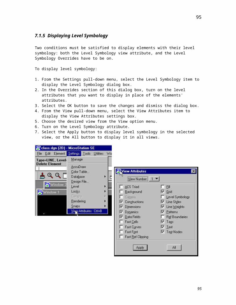
The Undo Other Item
This item also allows you to undo drawing operations. The difference is that instead of just undoing the last operation, you can undo all operations or operations back to a mark that you had previously set. The arrowhead beside the item name indicates that there is a sub-menu associated with it. From this sub-menu, you can choose to undo all your operations or undo operations back to a mark that you set. The illustration of the previous page shows this sub-menu.
The Redo Item keyin: redo
The Redo item negates the last Undo operation you performed, but it has to be selected immediately after undoing. If you execute another drawing tool after undoing an operation, you lose the redo ability for that undo. When you enter the Edit menu, the operation that will be redone will automatically display beside the Redo item. You can redo a series of negated operations by repeatedly choosing Redo. The redo operation can also be performed by issuing a <Ctrl-R> in the Command Window.
The Set Mark Item
The Set Mark item allows you to set a mark in your undo buffer. Now if you select the item Undo Other> To Mark, you will be able to undo all operations back to your mark.
95

8.1.6 Element Information/Analyze
Opens the Element Information settings box, which is used to change the attributes of an element(s) and review design file data associated with them, such as geometry and database attributes.
keyin: ana a single element is selected when Information is chosen, the displayed data pertains to that element. If a complex element is selected, the displayed data pertains to the first element selected, if the elements were selected individually, or otherwise to the element stored closest to the beginning of the design file. To advance to the next element, click the Next button. (If there are no selected elements, you are prompted to identify an element. After you do so, the settings box opens.)
The element type and type number are shown in the title bar.
Element data
Shows the element's geometry, tag values, database attributes, and attributes specific to the element type.
Element text
96
(Displayed only if the element is a text or text node element) Sets the element text. You may not remove all the text.
NOTE: If the element is a text node, only one line of text can be edited at a time.
Next
Displays data for the next selected element or the next component element of a complex element. Next is disabled (dimmed) if the element is the last selected element or if the only selected element is a complex element, is its last component.
NOTE: The notation, "x of y," in the upper left-hand corner of the settings box indicates the number of components (y) including the "header," and the relative position of the component for which information is shown (x). The nesting level of the complex element is shown in parentheses to the right of the element type number.
Previous
Displays data for the previous selected element or the previous component element of a complex element. Previous is disabled (dimmed) if the element is the first selected element or if the only selected element is a complex element, is its "header."
Apply
Applies changes to the element's attributes. An alert box opens to inform you that changes cannot be undone and asks you to confirm the changes.
97
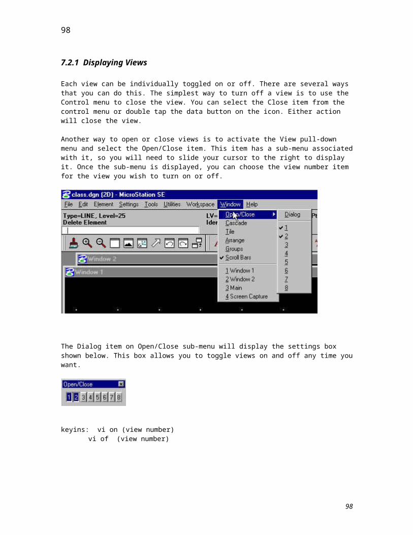
8.2 Precision Input
There are several precision input options available to place features precisely in map files. The XY, DL, and DI keyins will be profiled in the following sections.
98
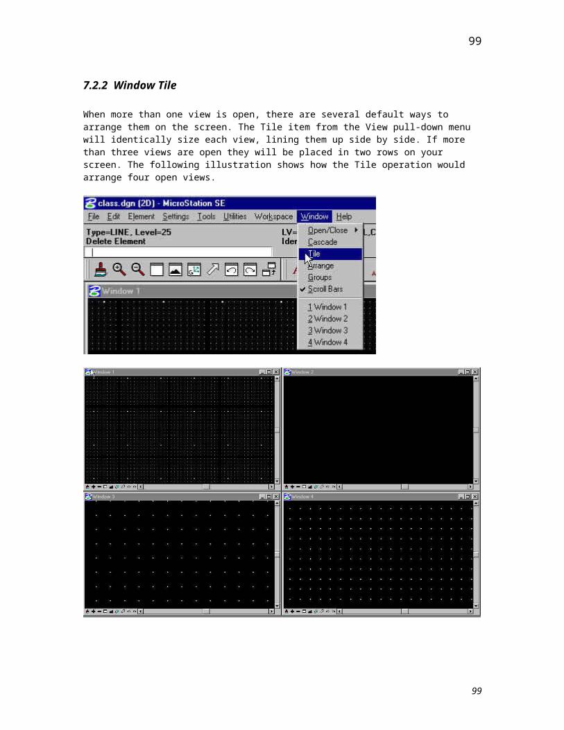
8.2.1 XY=
keyin: xy= (x coordinate, y coordinate) [ | times repeated]
MicroStation allows you to place data points by specifying their coordinate positions. This feature is most frequently used to indicate the exact position for a point features origin point. The key-in command that you use to specify coordinate positions is xy=.
The values for the X and Y coordinates should be specified in working units format, but they can be either a positive or negative value. The optional portion of this key-in allows you to specify the number of times it is to be repeated. This option is helpful for defining a center point for placement of multiple elements. If you wish to use this option, follow the Y coordinate with a pipe symbol and the number of times you want to repeat the key-in.
You want to create a line that's origin point is the global origin of the design. Here are the steps you would follow to create this line:
1. Select the Place Line tool.2. Key in xy=0,0 in the Input field of the Command Window.3. Complete the command by entering a data point to visually select the line's end point or enter another
xy= key-in to specify the exact coordinates for the line's end point.
NOTE: The xy= key-in uses the drawing coordinate system. So the coordinates you enter are always placed relative to the global origin.
99

8.2.2 DX= and DL=
keyins: dx= (delta x, delta y) [ | times repeated]dl= (delta x, delta y) [ | times repeated]
You can use the dx= and dl= key-in commands to place a data point at an exact rectangular offset distance from a previous data point or current tentative point.The delta values for X and Y are entered in working units format and they can be positive or negative. Once again, the optional times repeated portion is useful for placing multiple elements.
The only difference between these two key-ins is that dx= uses the view coordinate system and dl= uses the drawing coordinate system. Unless you are working in a rotated view in a 3-D file, you will not see a difference between these two key-ins.
For example, you want to create a line that is 10.5 feet in length, and it's origin point is 5 feet to the right of an existing element. Here are the steps needed to create this line:
1. Select the Place Line tool.2. Use the tentative button to snap to the right side of the existing element.3. Key in dx=5,0. This indicates that you want the origin point of the line to be 5 feet to the right of the
current tentative point.4. Key in dx=10:6,0. This indicates that the end point for the line is 10 feet 6 inches from the previous
data point.
NOTE: By default, the active snap mode for a MicroStation design is the Keypoint snap mode. This means that when you use the tentative button to snap to an element, MicroStation will automatically locate one of the keypoints of that element. (Keypoints are usually located at element endpoints, vertices, and/or centers.)
100
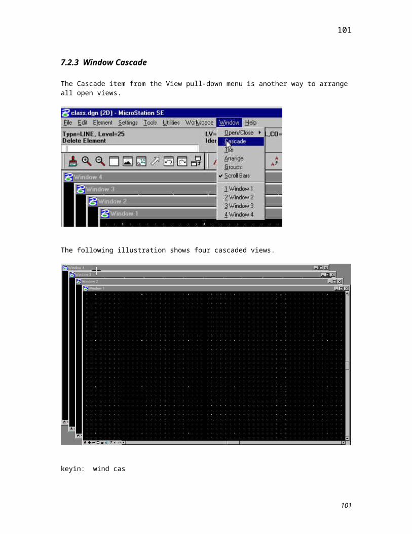
8.2.3 DI=
keyin: di= (distance, direction) [ | times repeated]
The di= key-in will also allow you to place a data point by referencing a previous data point or a current tentative point. The difference is that you can not only specify the distance, but also the angular direction of the next data point.
With this key-in, like the others, distance is entered in working units format. The difference is that it is followed by the direction or angle of placement that you desire. Valid angle values range from 0 to 360. They can be whole numbers or decimal values down to one ten-thousandth of a degree.
For example, you want to create a rectangle that is exactly 2 feet wide and 3 feet high. Here are the steps needed to create this rectangle:
1. Select the Place Line tool.2. Enter the origin point for the rectangle. You might do this by visually selecting a data point, entering
xy= to specify the exact coordinates, or by entering dx= to offset from the previous data point or current tentative point.
3. Key in the following to draw the rectangle:di=2,0di=3,90di=2,180di=3,270
NOTE: This key-in uses the view coordinate system, so the angle is always relative to the screen orientation, not the file's axes.
8.2.4 AccuDraw
To start AccuDraw, select the AccuDraw tool as shown below. The AccuDraw window appears.
Type <P> with the cursor in the AccuDraw window and the Data Point Keyin appears.
101
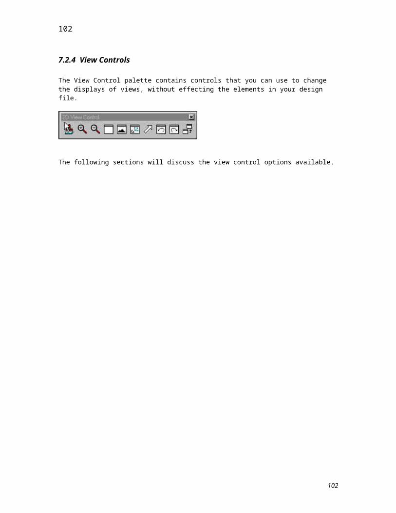
8.3 Snap Locks
Snapping allows you to put a tentative point directly on an existing element. Using tentative point snapping in conjunction with precision input commands helps you accurately construct new elements that are either connected to, or precisely related to existing ones. In MicroStation, tentative point snapping is affected by the current snap mode. By default, the Keypoint mode of snapping is enabled.
Keypoint snapping forces tentative points entered on or near existing elements to the nearest Keypoint on that element. A Keypoint is a regularly-spaced point in an element to which a tentative point will snap. The following figure shows the position of the default keypoints for many common element types.
If the Snap Lock is off, tentative points do not snap to elements, they only display the coordinates of the point. When this lock is on, tentative points will snap to elements. Where on the element they will snap is determined by the current snap mode. There are two methods that you can use to toggle the Snap Lock setting.
The first method is the Locks settings box. This box is displayed by activating the Settings pull-down menu and selecting the Locks item to display its associated sub-menu. From this sub-menu, select the Full item. Once the Locks settings box is displayed, you toggle the Snap Lock on or off by selecting the Snap Lock check button/box.
The second method is the Lock Toggles settings box. This box is also displayed by activating the Settings pull-down menu and selecting the Locks item to display the associated sub-menu. But, this time select the Toggles item from the sub-menu. To toggle the Snap Lock on or off, select the Snap Lock check button/box.The following illustration shows both settings boxes with Snap Lock enabled.
102
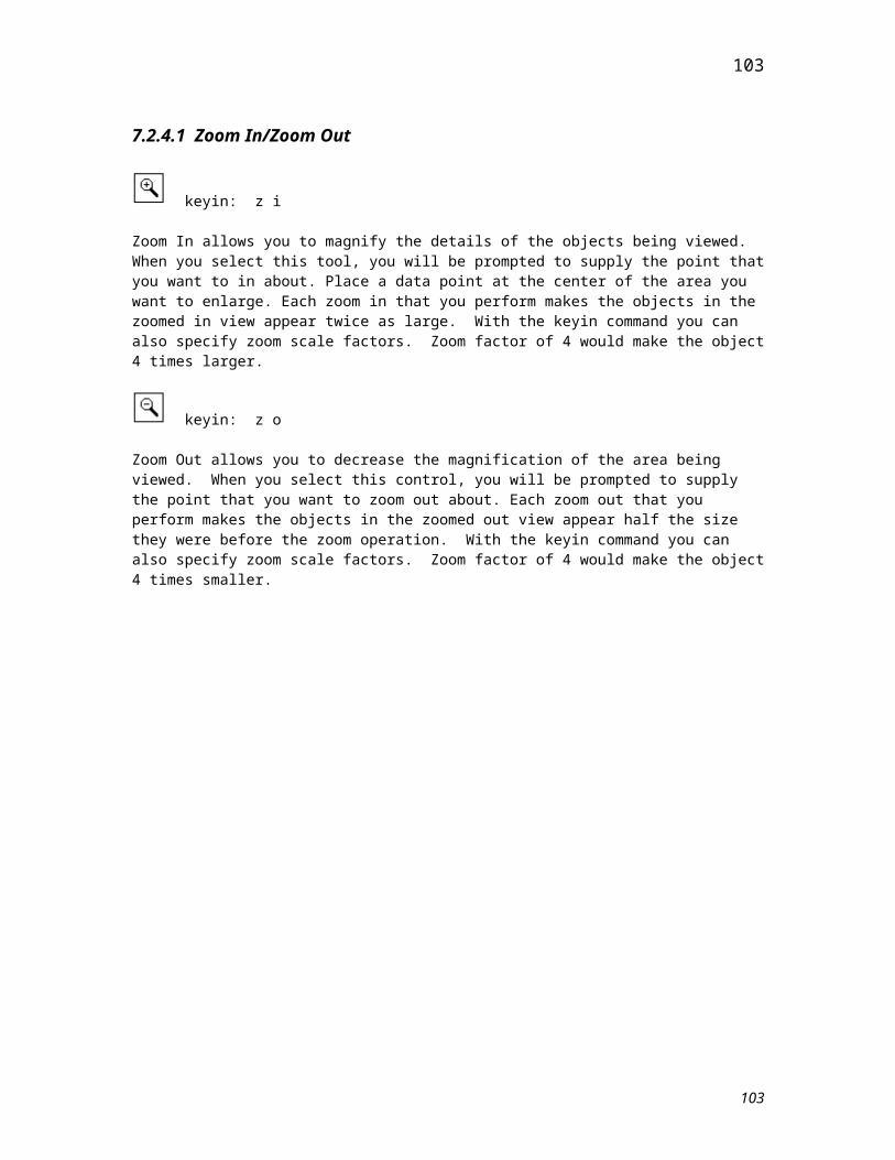
103
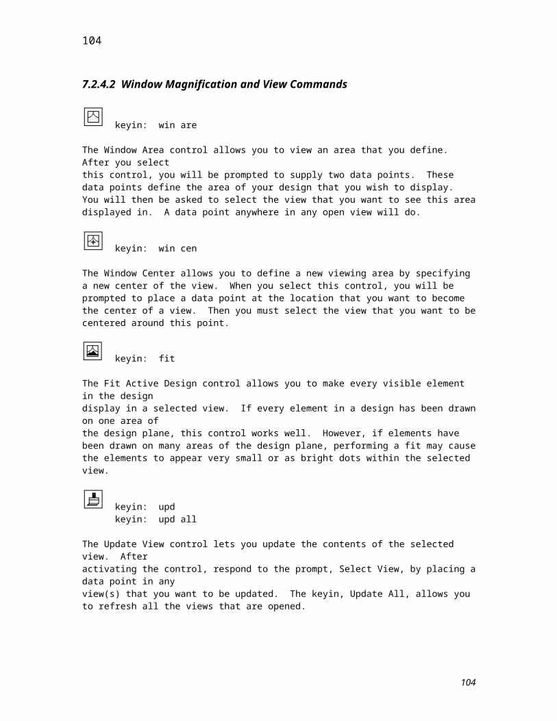
8.3.1 Keypoint Snap
keyin: lock sn key
The Keypoint Snap Lock allows you to snap to the nearest keypoint on the element. The following illustration shows the effect of the Keypoint snap. The arrow represents the cursor position when the tentative point is issued. The large cross and circle displays to show the position that is snapped to.
NOTE: Keypoints are regularly spaced points on an element that a tentative point can snap to. The number of keypoints an element has is determined by the element type and the Snap Lock Divisor (KY=). The default divisor for MicroStation 5.0 is 2. The following table lists the location of the minimum keypoints for some of the common element types.
104
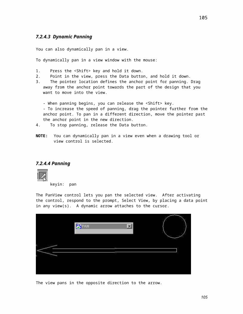
8.3.2 Nearest Point Snap
keyin: lock sn pro
The Nearest Point Snap allows you to snap to the point on the element that is nearest to the pointer. The illustration below shows the effect of the Nearest Point Snap lock.
105

8.3.3 Intersection Snap
keyin: lock sn int
The Intersection Snap allows you to snap to the intersection of two elements (this mode requires at least two tentative points.) The first tentative point will snap to an element, and that element will highlight. The second tentative point will snap to another element, and the two segments used to find the intersection will display in dashed lines. The illustration below shows the effect of the Nearest Point Snap lock.
106

Lesson 9 - Grouping Techniques
There will be times when you will want to perform the same operation on several elements. This can be done by repeating the operation for each individual element, or by temporarily grouping the elements and performing the operation once for the entire grouping. This lesson covers three different ways that you can create these temporary groupings in MicroStation. Covered will be the usage of fences, selection sets, and graphic groups.
107
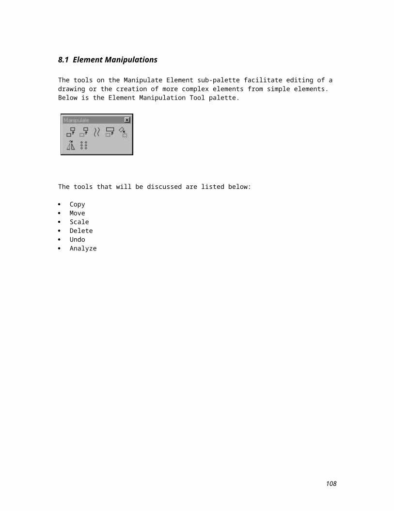
9.1 Fences
One way that you can group elements in your design file is to place a fence around them. Once a fence has been placed, you can move, copy, scale, spin, delete, or change the attributes of elements that are in the fence. There are three important things that you need to remember about fences:
A fence is a temporary structure that you can use to group elements. It is not an element and it is not saved as part of your design. Only one fence can exist in your design file at any given time.
MicroStation fences can be in one of six different modes. These modes determine which elements are considered to be fenced. You can set the fence mode when you create the fence, when you perform any operation that uses the fence, or at any time from the Locks settings box.
The available fence modes are:
Inside - When this mode is selected, only elements that lie entirely inside the fence will be affected. Overlap - With this mode, elements that lie inside or elements that overlap any portion of the fence
will be affected. Clip - This mode is similar to the Overlap mode, it too will effect elements that lie inside the fence or
ones that overlap any portion of the fence. The difference is that Clip mode will actually break overlapping elements at the points where they touch the fence. So only the portions of the broken elements that lie inside the fence will be effected. It is important to realize that any element that is broken by a fence clip operation no longer maintains its original element properties.
Void - When this mode is selected, only elements that lie entirely outside the fence will be affected. Void Overlap - With this mode, elements that lie outside or elements that overlap any portion of the
fence will be affected. Void Clip - This mode is just the opposite of the Clip mode. Any elements that lie totally outside the
fence will be affected, and any elements that overlap the fence will be clipped and the portions that lie outside the fence will be affected. Once again, it is important to realize that any element broken by a fence clip operation no longer maintains its original properties.
108
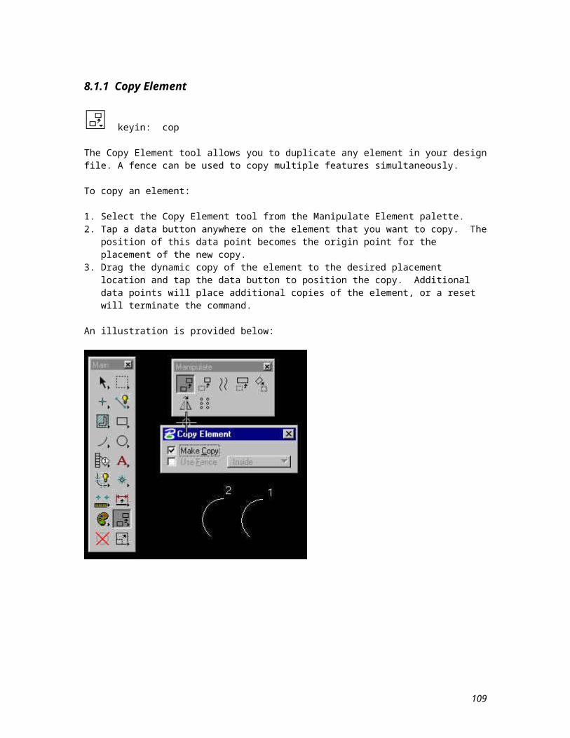
9.1.1 Fence Sub-Palette Options
You can use the tools on the Fence sub-palette to place, modify, or move a fence. There is also a tool that allows you to delete the elements in the fence. No matter which Fence tool is active, the Fence Mode option menu will always be available for you to select the desired fence mode.
The Fence sub-palette options are described below.
keyin: pla fen
The Place Fence Block tool allows you to place a rectangular fence. When you activate this tool, you will be prompted to supply two data points. These data points will be the diagonal vertices of your fence.
keyin: pla fen sha
The Place Fence Shape tool is also used for placing fences, but it allows you to determine the fence's shape. When you select this tool, you will be prompted to enter data points to define the shape of your fence. You can close your fence by selecting the Close Fence button from the tool settings area or by entering a data point that is close to the original data point.
109
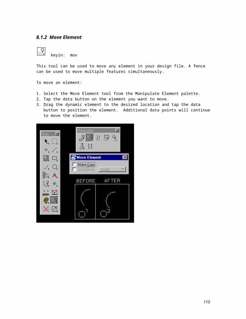
keyin: mod fen
The Modify Fence Vertex tool allows you to change the vertices of your fence. After you select this tool, tap the data button on the vertex that you wish to change, move the mouse until the dynamic vertex appears in the correct position, tap the data point again to position the vertex, and tap the reset button to complete the operation.
keyin: mov fen
The Move Fence Block/Shape tool allows you to move your fence. It is important to realize that this action will move the contents of the fence. You can set Copy, Move, Rotate, Scale, Mirror, Stretch for fence contents. After you select this tool, tap the data button on the fence, move the cursor until the dynamic fence appears in the correct location, tap the data button again to position the fence, and tap the reset button to complete the operation.
keyin: fen del
The Delete Fence Contents tool, unlike the other tools on this palette, will affect the elements within the fence. When you select this tool, you will be prompted to confirm the deletion with a data point. A data point anywhere in an open view will confirm this action and delete the contents of the fence. Remember that the current fence mode will determine which elements will be deleted.
110
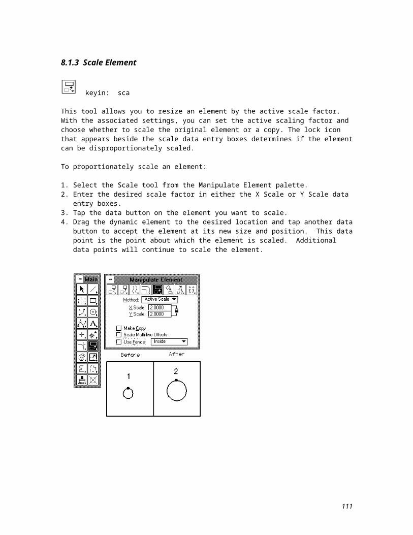
9.1.2 Fence Operations
The following example outlines the steps necessary to change the element attributes of elements that have been grouped with a fence.
To change element attributes using a fence:
1. Select either the Place Fence Block or the Place Fence Shape tool from the Fence palette.2. Select the desired fence mode from the Fence Mode option menu. This can be done in the Fence
palette if it is floating or in the Tool Settings box.3. Enter the data points needed to place the fence.4. Select the Change Element Attributes tool from the Change Element palette.5. In the Change Element Attributes tool settings box, chose the following options:
- Select the check button/box beside all the attributes that you wish to change, and enter the new settings from the associated option menus or data entry boxes.- Select the check button/box Use Fence. Notice that you can also select the fence mode from the option menu that displays beside this check button/box.
6. Enter a data point anywhere in your view to accept the change and the elements are redrawn with the new attributes.
111
The following illustration shows the palettes that are needed to perform the operation outlined above.
112
9.2 Selection Sets
Another way to temporarily group elements is to use the Element Selection tool found on the Main palette. This tool allows you to select a single element, a group of elements, or all elements that lie within a specified area. When an element or group of elements has been selected with this tool, handles will display around the element(s). The element(s) can now be changed or manipulated the same way you would change or manipulate any single element.
NOTE: There are many special manipulations that can be performed on elements that have been selected with the Element Selection tool. Consult the MicroStation Reference Guide for more information on this topic.
113
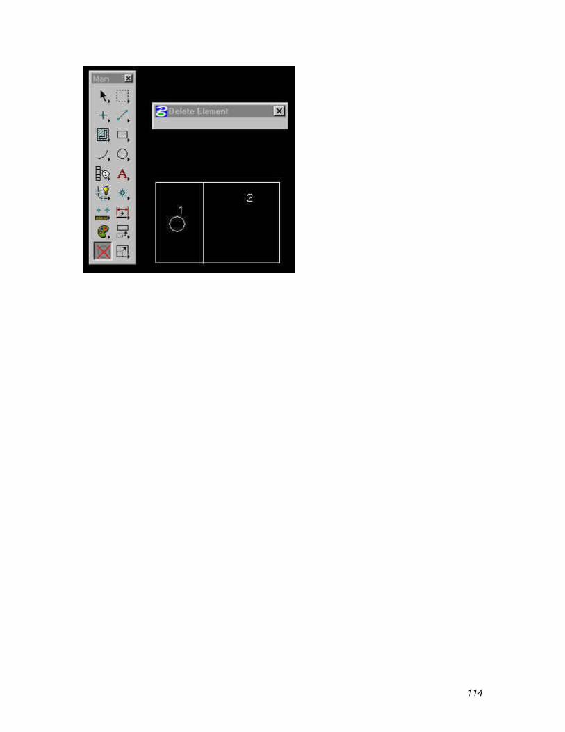
9.2.1 Single Element Selection Sets
keyin: cho el
To select a single element:
1. Select the Element Selection tool from the Main palette.2. Tap a data button on the desired element. The element will now display with handles indicating that it
is the current selection element.
The following illustration shows an element that has been selected with this tool. Notice that only the first section of the line displays with handles. This is because it was created with the Place Line tool, so the Element Selection tool sees this line as three separate line segments, rather than one element.
The line string in this illustration was created with the Place Line String tool. So the Element Selection tool recognizes that it is one element and displays handles accordingly.
114
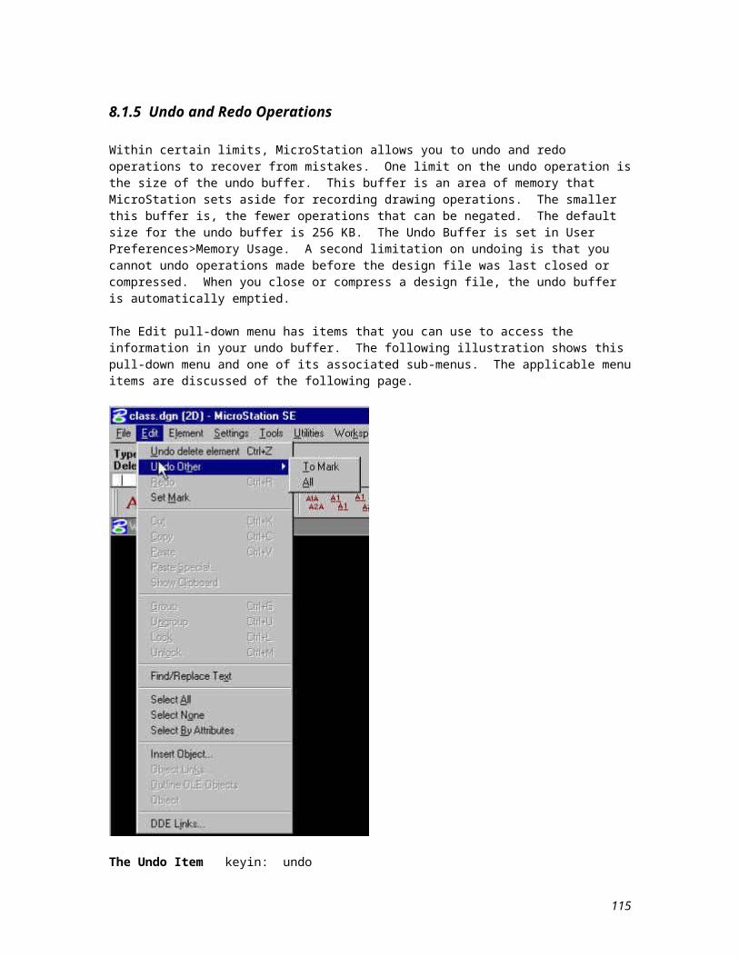
9.2.2 Multiple Element Selection Sets
To select multiple elements:
1. Select the Element Selection tool from the Main palette.2. Press and hold the <Ctrl> key on the keyboard and tap the data button on the desired element.
Continue this process until all the desired elements are selected.
NOTE: In the Element Selection tool, the sequence <Ctrl> key - data button is a toggle. If you issue this sequence on an element that has already been selected, you will be un-selecting it.
The following illustration shows three elements from a design file. Two of these elements, the block and the line string, have been selected with the Element Selection tool. These elements can now be changed or manipulated as if they were one element.
115

9.2.3 Selection Sets within an Area
To select all the elements within a specified area:
1. Select the Element Selection tool from the Main palette.2. Position the screen cursor at one corner of the area that you want to select, press and hold the data
button, drag the dynamic fence to the opposite corner of the area, and release the data button. All elements that lie completely inside this area will now display with handles indicating that they are selected.
The following illustration shows the same three design elements as before. This time the line string and the block were selected with the specified area method instead of being selected individually. The dashed block shown in this illustration represents the area that was defined with the Element Selection tool. Notice that the circle was not selected since it did not lie completely inside the area.
NOTE: If you hold the <Ctrl> and the <Shift> keys while you are dragging across elements, any element that lies inside or overlaps the defined area will be selected.
116
9.3 Graphic Groups
Another grouping technique that is available in MicroStation is the graphic group. Graphic groups allow you to add, remove, and manipulate individual members without breaking up the grouping. This makes it the most flexible grouping technique available. There is also a Graphic Group Lock which determines whether your actions affect all or only portions of the grouping.
The Chain sub-palette contains tools for creating a graphic group, and for adding and removing graphic group members.
The following sections will present commands relevant to the construction and manipulation of graphic groups.
117
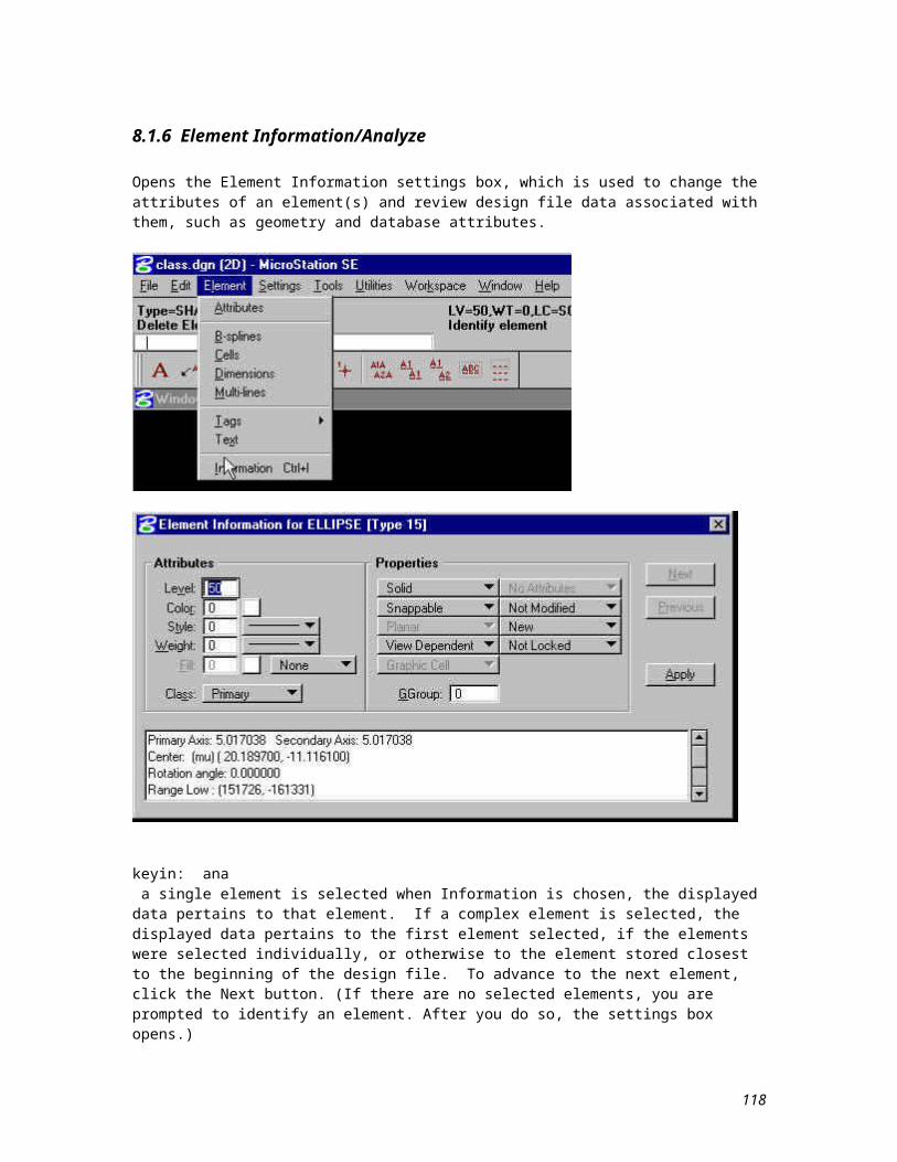
9.3.1 Creation of a Graphic Group
keyin: gro add
To create a graphic group or add elements to a graphic group:
1. From the Chain sub-palette, select the Add to Graphic Group tool.2. Identify the first element.
If this element is not a member of a graphic group, a new graphic group is created.If this element is a member of a graphic group, all elements subsequently identified are added to the graphic group.
3. Identify other elements to add to the graphic group.If an identified element is already a member of a separate graphic group, all of the elements in that graphic group are added to this graphic group.
4. Accept the graphic group.
Once a graphic group has been created, the Graphic Group Lock determines whether manipulations affect the entire group or individual members. This lock can be enabled or disabled from either the Locks settings box or the Lock Toggles settings box. If the Graphic Group Lock is enabled, any manipulation that is performed will affect the entire graphic group. If it is disabled, the member elements can be manipulated individually.
keyin: lock gg
118
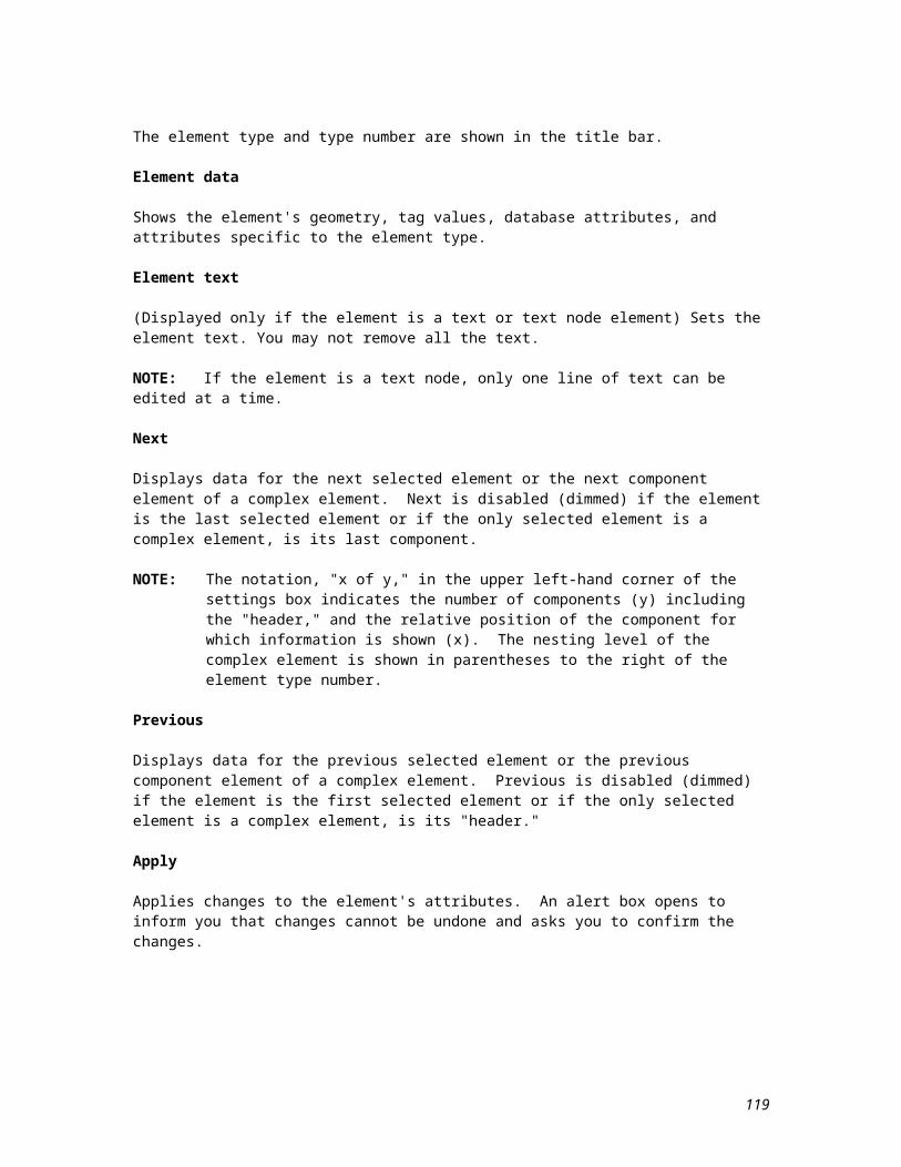
9.3.2 Dropping Graphic Groups
keyin: gro dro
To remove elements from a graphic group:
1. From the Locks settings box, turn off the Graphic Group Lock.2. From the Chain sub-palette, select the Drop from Graphic Group tool.3. Identify the element(s) to be dropped from the graphic group.4. Accept the drop.
To break up an entire graphic group:
1. From the Locks settings box, turn on the Graphic Group Lock.2. From the Chain sub-palette, select the Drop from Graphic Group tool.3. Identify a member of the graphic group.4. Accept the drop.
119

Lesson 10 - Modifying Features/Elements
This lesson will cover the modification of map features. Features can be modified from four different sub-palettes: Manipulate Element, Modify Element, Construct Fillet, and Group. Both of these palettes are accessed from the Main palette or the Command Window menu. The palettes are displayed below.
The following sections will discuss the specific commands that are most frequently used in generating and editing feature data in map files.
120
10.1 Modify Element
keyin: mod
The Modify Element tool can be used to perform the following operations:
Move a vertex of a line, line string, multi-line, curve, B-spline control polygon, shape, complex chain, or complex shape.
Scale a block. Change the radius of a circle or the length of one axis of an ellipse. Move dimension text or modify the extension line length of a dimension element.
To modify an element:
1. From the Modify Element palette, select the Modify Element tool.2. Identify the element close to the vertex or axis you want to modify.3. Move the cursor until the dynamic element takes the shape and/or size that you desire, then enter a data
point to accept the modification.
NOTE: The Arcs sub-palette contains additional tool for modifying arcs.
In the following illustration, the Modify Element tool is used to change a line representing a linear feature in a file.
121
10.2 Partial Delete Command
keyin: del par
This tool allows you to delete a portion of an element. A closed element is turned into an open element. So an ellipse or circle becomes an arc; a shape becomes a line string; a closed B-spline curve or multi-line becomes an open B-spline curve or multi-line. If an interior portion of an open element, such as a line, line string, multi-line, curve, or arc, is partially deleted, the element is divided into two elements of the same type.
To delete part of an element:
1. From the Modify Element palette, select the Delete Part of Element tool.2. Enter a data point to select the element and the starting point of the portion to be deleted.3. For an open element, enter a second data point to identify the endpoint of the portion to be deleted.
For a closed element, enter a second data point to define the direction in which to delete. Then enter a third data point to define the endpoint of the portion to be deleted.
In the following illustration, one portion line is deleted. The line shown here is an open element.
The following illustration shows the data points that would be needed to partially delete a closed shape.
122
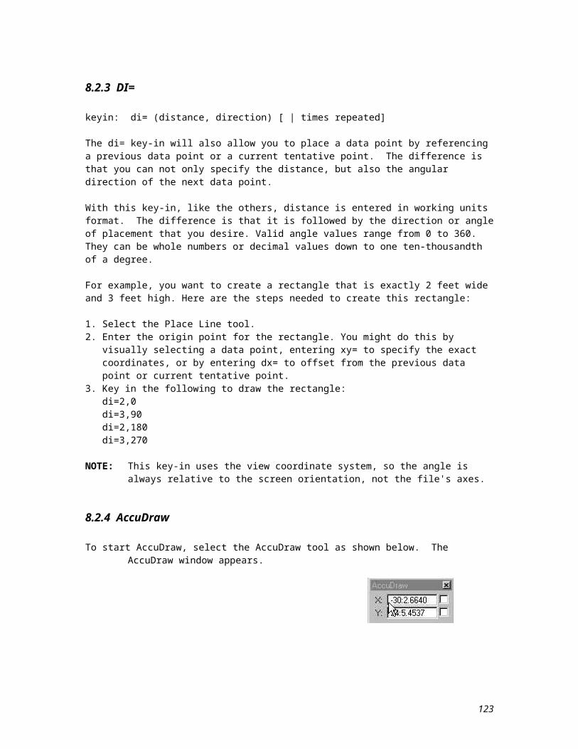
123
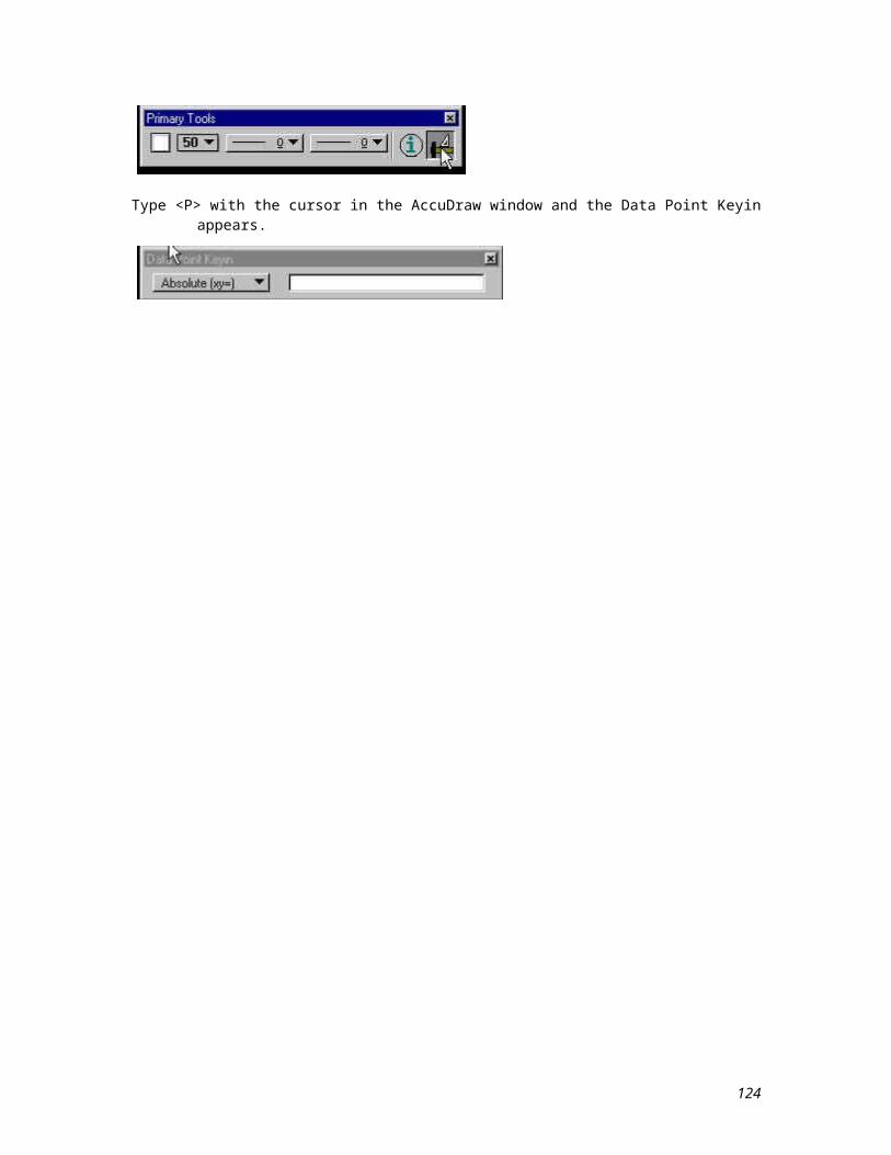
10.3 Extend Line
keyin: ext lin
The Extend Line tool allows you to extend or shorten existing lines or end segments of a line string or multi-line. The Distance setting associated with this tool gives you the option of specifying an exact distance to lengthen or shorten the line. A negative distance shortens the line, and a positive distance extends the line.
To extend or shorten a line:
1. From the Modify Element palette, select the Extend Line tool.2. If an exact distance is desired, select the Distance check button/box and enter the distance in the
associated data entry box.3. Identify the line near the endpoint you want to modify.4. If Distance is on, enter a second data point to accept the modification.
If Distance is off, enter a second data point to graphically extend the line.
The following illustration shows the line being extended and the new endpoint graphically defined.
124
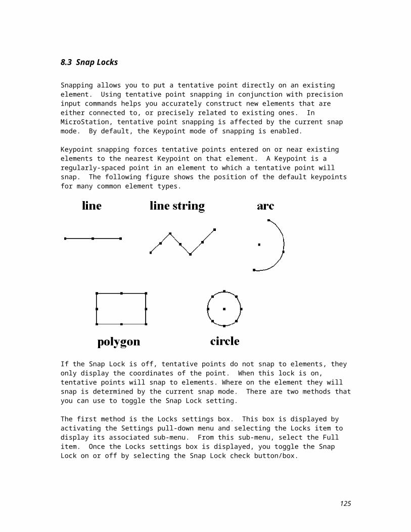
10.4 Extend Two Elements
keyin: ext lin 2
You can use this tool to extend or shorten two open elements to their intersection.
To extend two elements to their intersection:
1. From the Modify Element palette, select the Extend Two Elements to Intersection tool.2. Enter a data point to identify the first element. When an element is shortened, the part of the element
that is identified is kept. 3. Enter another data point to identify the second element. The dynamic elements will then be extended
to their intersection. No modification is made if the identified elements cannot be extended or shortened so that they intersect.
4. Enter a third data point to accept the intersection.
The following illustration shows the extension of two lines to their intersection.
125

10.5 Extend Element to Intersection
keyin: ext lin int
This tool can be used to extend or shorten a line, line string, or arc to its intersection with another element.
To extend one element to its intersection with another element:
1. From the Modify Element palette, select the Extend Element to Intersection tool.2. Enter a data point to identify the element you want to extend or shorten.3. Enter another data point to identify the element to which the first element will be extended or
shortened. 4. Enter a third data point to accept the modification.
In the following illustration, the line element is extended to its intersection with an arc. Notice that neither the size, nor the position of the arc is changed.
126
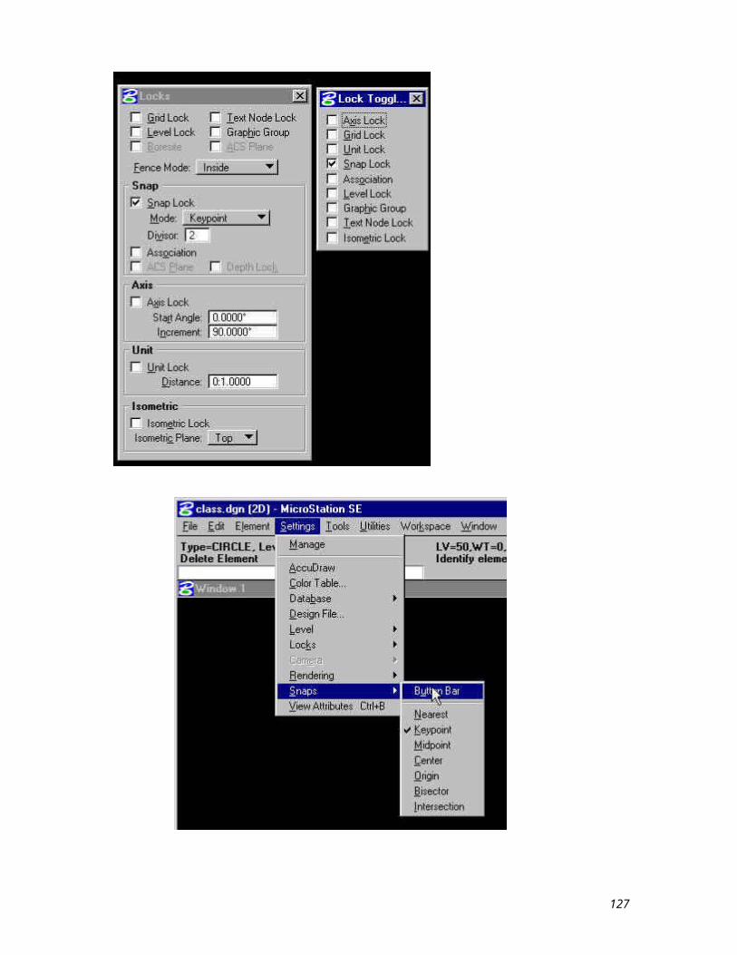
10.6 Trim
keyin: tri
This tool is used to trim a series of elements at their intersection with one or more other elements. The cutting element and the elements that are trimmed can be lines, line strings, arcs, curves, B-spline curves, shapes, ellipses, complex chains, or complex shapes.
To trim elements:
1. From the Modify Element palette, select the Trim Element tool.2. Enter a data point to identify the cutting element.3. Enter another data point to identify the first element that you want to trim (the part of the element
identified will be the protion that is trimmed away). The element is highlighted and how it will be trimmed is dynamically displayed.
4. Enter a third data point to accept the trimmed element. 5. Go back to step 3 to identify another element to trim,
or Enter a reset to stop the trim operation.
In the following illustration, the vertical line is identified as the cutting element, so any portion of an element that falls to the right of it is trimmed.
127
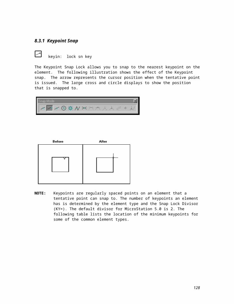
10.7 Insert Vertex
keyin: ins ver
You can use this tool to insert a vertex in a line, line string, multi-line, shape, or B-spline control polygon. It can also add an extension line to a dimension element.
To insert a vertex:
1. From the Modify Element palette, select the Insert Vertex tool.2. Enter a data point to identify the segment on which you want to insert a vertex.3. Position the dynamic vertex and enter a data point to accept it.
The following illustration shows the insertion of a vertex in a block element.
128
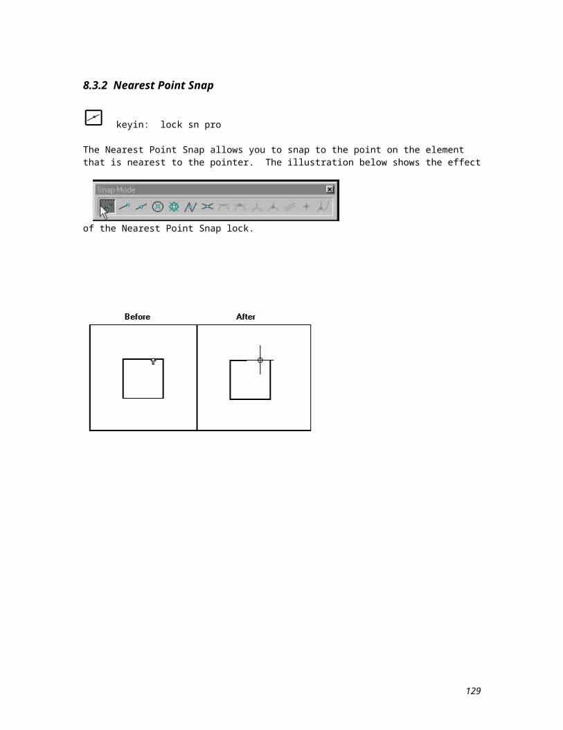
10.8 Delete Vertex
keyin: del ver
This tool can be used to delete a vertex from a line string, multi-line, shape, or B-spline control polygon, or to remove an extension line from a dimension element.
To delete a vertex:
1. From the Modify Element palette, select the Delete Vertex tool.2. Enter a data point to identify the vertex that you want to delete.3. Enter another data point to accept the vertex deletion.
The following illustration shows the deletion of one vertex of a block element.
129
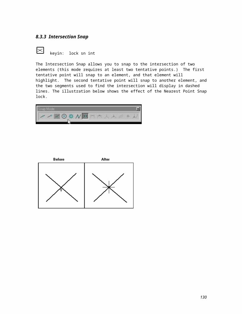
10.9 Rotate Element
keyin: rot
This tool allows you to rotate an element or copy of an element. You can chose the rotation angle graphically with a data point, or you can enter a specific angle through the associated settings.
To rotate an element at a specified angle:
1. Select the Rotate tool from the Manipulate Element palette.2. Select the By Active Angle check button/box and enter the desired angle in the associated data entry
box.3. Use a data button to identify the element you want to spin. 4. Enter another data point to accept the identified element. This data point becomes the pivot point for
the rotation.5. Rotate the dynamic element to the desired location and enter a data point to position it. Additional
data points will continue to rotate the element.
Below is an illustration of rotating a shape.
130
10.10 Copy Parallel
keyin: cop par and cop par key
The Make Copy setting associated with this tool allows you to chose if you want to move the original element or a copy. Also, the Distance setting allows you to specify the parallel distance that the element will be moved or copied. The following steps outline one way of using this tool.
To copy an element at a specified parallel distance:
1. Select the Move Parallel tool from the Manipulate Element palette.2. Select the Distance check button/box and enter the desired distance in the associated data entry box.3. Select the Make Copy check button/box.4. Tap the data button on the element you want to copy.5. Enter another data point to indicate the direction for the copy. Additional data points will place
additional copies, they will always be parallel and at the specified distance.
Below is an illustration of the Copy Parallel tool.
131
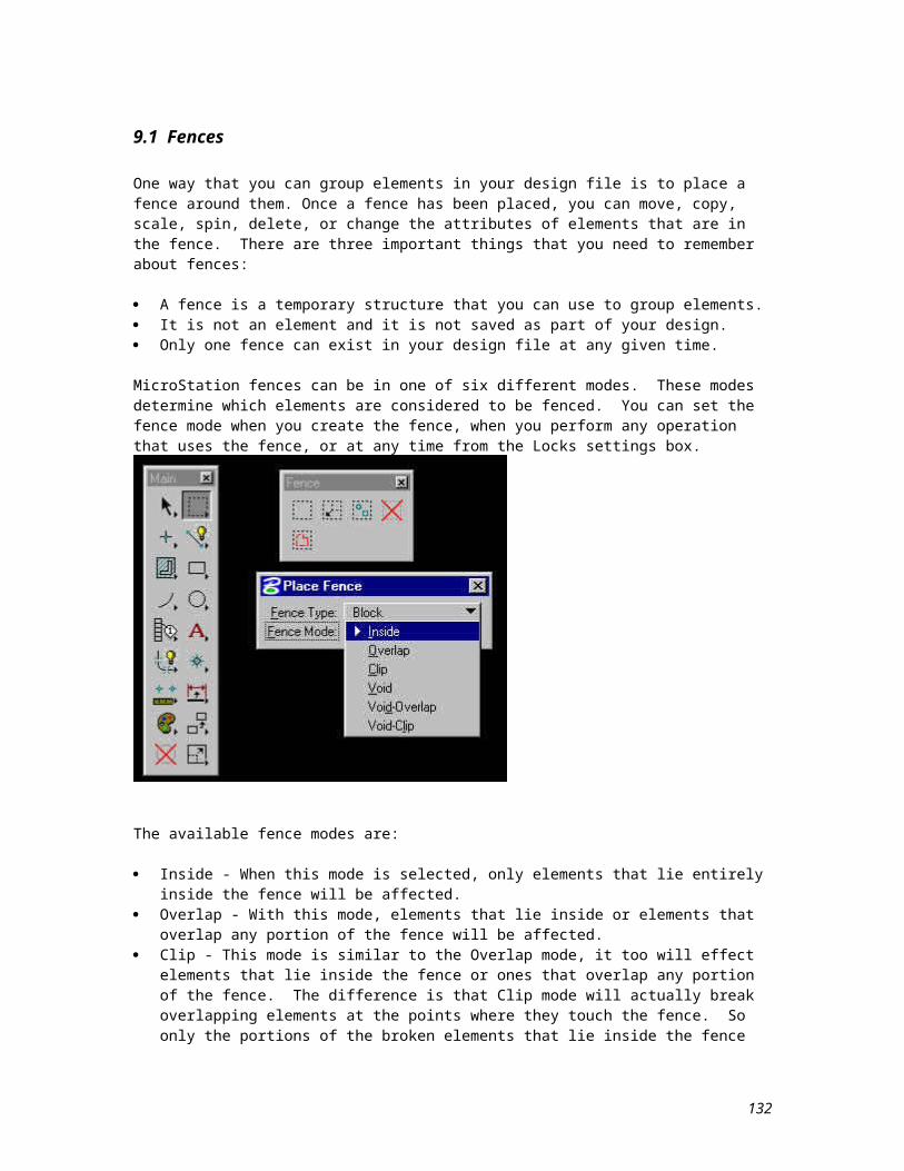
10.11 Construct Circular Fillet
keyin: fill mod
This tool is used to construct an arc between two elements, two sections of a line string, or two sides of a shape. Fillets can be created between lines, line strings, circular arcs, circles and shapes. If the fillet is constructed between two closed elements, or one open and one closed element, the closed element(s) are not modified.
There are two settings associated with the Construct Circular Fillet tool. They are:
Radius - You can enter the desired radius for the fillet in this data entry box. Truncate - You can control which side(s) of the original elements are truncated with this option menu.
The choices you have are:- None - Neither side is truncated.- Both - Both sides are truncated at their point of tangency with the fillet.
- Single - Only the first side that is identified is truncated. It will be truncated at its point of tangency with the fillet.
The illustrations on the following pages show the steps necessary to create circular fillets and perform two different types of modifications.
To construct a circular fillet and truncate both elements:
1. From the Fillets palette, select the Construct Circular Fillet tool.2. In the Radius data entry box, enter the desired fillet radius.3. From the Truncate option menu, choose the Both option.4. Enter a data point to identify the first element or segment.5. Enter a second data point to identify the second element or segment.6. Enter a third data point to accept the fillet and truncations.
132
The following illustration shows the construction of a circular fillet between two lines. Both lines will be truncated with this operation.
133
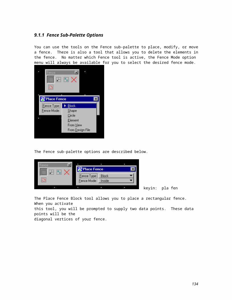
10.12 Create Complex Chain
keyin: cre cha
This tool is used to combine individual elements into a single open complex chain. This chain can then be manipulated as a single element. Once the complex chain is defined, it takes on the current active element attributes and any former element attributes are discarded. There are two settings associated with this tool that determine how elements are added to the chain. They are:
Method - From this option menu, you can determine how elements are added to the chain. The two available methods are:
- Manual - With this method, you must manually identify each element that you want to become part of the chain.
- Automatic - With this method, you can let MicroStation automatically identify elements to be added to the chain. You must identify and accept the first element, then if an endpoint of an additional element is within a specified distance of your original element, it will automatically be selected. All you have to do to add this element to your chain is to accept it. This automatic selection will continue until there are no more elements within the specified distance, or you issue a reset.
Max Gap - This data entry box is where you specify the maximum distance between elements for the Automatic method of element selection. Distances should be entered in working units format. A distance of zero indicates that only elements that connect can be added to the chain.
To create a complex chain automatically:
1. From the Chain palette, select the Create Complex Chain tool.2. From the Method option menu, choose Automatic. Enter the maximum gap distance in the Max Gap
data entry box.3. Identify the first element to be added to the chain. 4. Enter another data point to accept this element. 5. Accept additional elements as they highlight. If the two elements do not meet, a filler line is
automatically added to force them together. If more than one element is within the Max Gap, the message "FORK -- Accept or Reset to See Alternate" displays in the Command Window. Enter a data point to accept the highlighted element or reset to highlight an alternate element. Continue to reset until the desired element highlights.
6. Once all the desired chain elements are selected and accepted, terminate the definition process by tapping the reset button. The definition process will automatically cease when no element is found within the Max Gap distance.
134
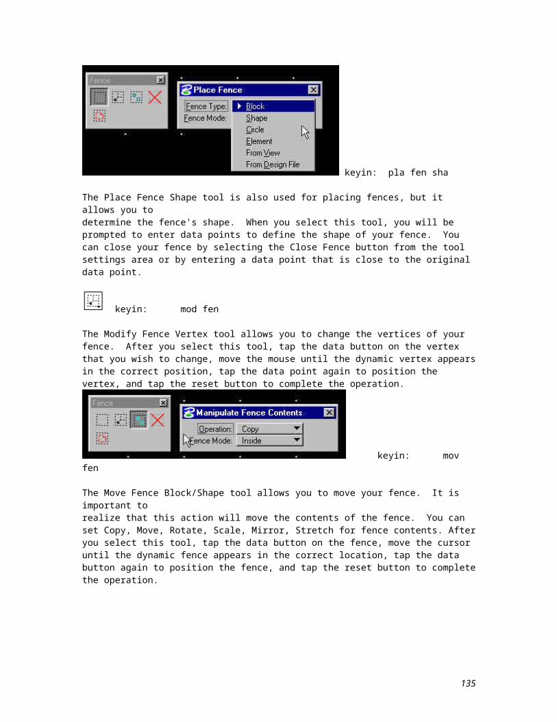
To create a complex chain manually:
1. From the Chain palette, select the Create Complex Chain tool.2. From the Method option menu, choose Manual.3. Identify the first element to be added to the chain. 4. You will then be prompted to accept this element and identify the next element.
If the two elements do not meet, they are automatically connected as they are identified. These connections appear as lines that connect the endpoints of the elements but are not elements. They disappear when complex status is dropped. It is recommended that elements be connected manually before being included in a complex chain.
5. Continue adding elements to the chain in sequence, either clockwise or counterclockwise, but not by random zigzagging.
6. Once all the chain elements are selected and accepted, terminate the definition process by tapping the reset button.
The following illustration shows the use of the Create Complex Chain tool Automatic method to chain together two lines and an arc.
135
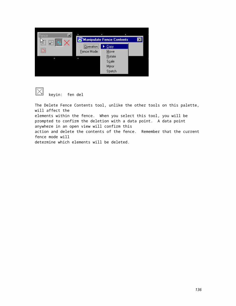
10.13 Create Complex Shape
keyin: cre sha
The Create Complex Shape tool is used to define individual elements as a closed complex shape. The resulting element is a closed complex element that can be manipulated as a single element. The area of the complex shape may be measured; but if the shape overlaps itself, there may be confusion about which portions are included in the shape to arrive at the overall area. Once the complex element is defined, it takes on the current active element attributes. There are several settings associated with the Create Complex Shape tool that determine how the complex shape is defined and what attributes it will have. These settings are:
Method - From this option menu, you can specify how elements are added to the complex shape. The available methods are:
- Manual - With this method, you can manually select lines, line strings, arcs, curves, and B-spline curves to be included in the complex shape.
- Automatic - With this method, lines, line strings, arcs, curves, and B-spline curves are automatically selected for inclusion in the complex shape if their endpoints are within the Max Gap distance.
Max Gap - This data entry box is where you specify the maximum distance between elements for the Automatic method of element selection. Distances should be entered in working units format. A distance of zero indicates that only elements that connect can be added to the shape.
Area - This option menu allows you to choose whether the created shape is a Solid or a Hole. Fill Type - You can select the fill type for your shape from this option menu. The available choices
are: None, Opaque, or Outlined. Fill Color - From this setting, you can choose the fill color for your shape. You can either enter the
color number in the data entry box, or select the desired color from the associated color palette.
To create a complex shape:
1. From the Chain palette, select the Create Complex Shape tool.2. Choose all the desired tool settings.3. Identify the first element to become part of the shape.4. Continue identifying and accepting elements to add to the shape. Select the elements in sequence,
either clockwise or counterclockwise, but do not zigzag at random. If the elements are not connected, they will automatically be connected as they are identified. These connections appear as lines that connect the endpoints of the elements. These connections are part of the complex shape but are not elements. They disappear when complex status is dropped. It is recommended that elements be connected manually before being included in a complex shape.
5. If the first and last element connect, accept the shape. If the first and last element do not connect, reset to close the shape and create a line element between their endpoints.
The following illustration shows the automatic creation of a complex shape from a series of lines and an arc with the fill type set to opaque.
136
137
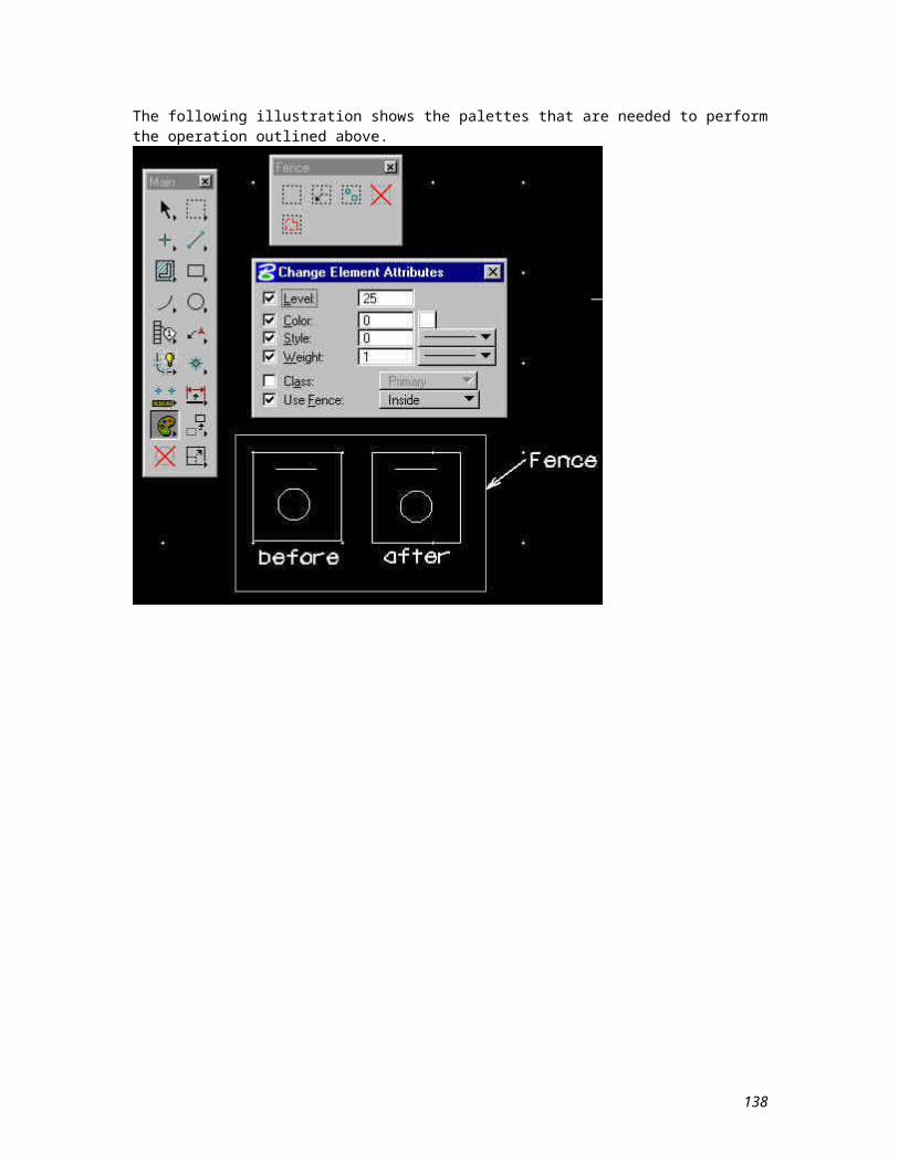
10.14 Drop Complex Status
keyin: dro
This tool can be used to drop a complex element into its primitive components. So a complex element like a cell, a complex chain, or a complex shape, is converted back to the individual elements that were used to create it.
If you have a complex chain or shape where connection lines were added to complete the element, there are two things you should be aware of:
These connection lines can not be used to identify the element. Once you drop complex status, the connection lines will no longer exist. You may need to update your
view to remove them from your display.
To drop a complex element into its primitive components:
1. From the Drop palette, select the Drop Complex Status tool.2. Enter a data point to identify the complex element that you want to drop.3. Enter another data point to accept that element.
138
Lesson 11 - Text
In this lesson you will learn all of the parameters and commands that impact the placement of text in a map file. Annotation is an important aspect of describing the features that reside in a map file.
Before any text is placed, MicroStation must have some settings defined to control the characters. The easiest way to specify these settings is through the Text settings box, like the one shown here. This settings box is displayed by selecting the Text item from the Element pull-down menu.
The major controlling parameters will be discussed in the following sections.
139
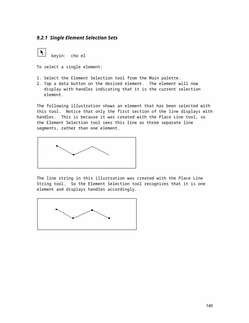
11.1 Fonts
keyin: sho fon (displays loaded fonts)ft= [font number] (sets active font)
The top portion of this settings box shows you what font, or character style, is currently active. You can use the items in this portion of the settings box to make a different font active. The characters that display in the Justification portion of this box, display in the active font, so you can see what your text will look like before you actually place it in your design file.
If you know the number of the font you want to use, you can enter it in the Font data entry box. If you don't know the number, you can use the associated option menu to pick a font from the list of available ones. You can also select the View button to display the Fonts settings box shown below.
The Fonts settings box displays more information about each of the available fonts. When you select a font from the list box, all the font's available characters will display, in that font, in the display area below the list box. If you tap a data button in this display area, the displayed font will become the active font.
140
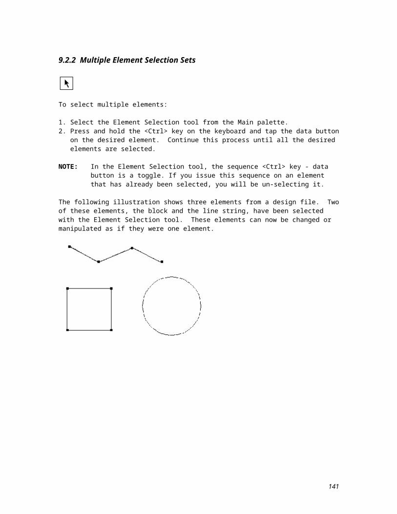
11.2 Text Justification
Justification is the orientation of a text element relative to the data point that is used to place it. The current text justification is shown graphically as a dark box in the active font display box. You can change the justification by tapping the data button in the area of this display box that you would like to be the new justification point.
The current justification also displays in two pairs of option menus below the active font display boxes. You can change the settings from these option menus also.
141
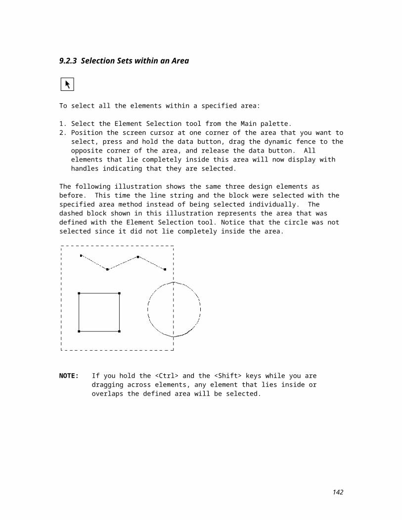
11.3 Text Size and Spacing
From the middle portion of the Text settings box you can specify the size and shaping for your text. The different options available are:
Height - You can specify the text height, in working units, in this data entry box.keyin: th=
Width - You can specify the text width, in working units, in this data entry box.keyin: tw=
The Lock Icon - If this icon is locked, the text height and width will be forced to be the same. If it is unlocked, you can change the two values independently.
Line Spacing - This data entry box is used to set the vertical spacing, in working units, between lines in a multi-line text element, or between text and the specified element when you choose to place text above, below, or along an element.
keyin: ls=
Line Length - You can specify the maximum number of characters allowed per line in a multi-line text element. This number cannot exceed 255.
keyin: ll=
Interchar Spacing - The distance, in working units, that you enter in this data entry field, will be the distance between each character.
Fractions - You can use this check button/box to indicate that fractions, numeric characters separated by a slash, should be treated as one character.
Underline - If you select this check button/box, your text will automatically be underlined.
Vertical Text - Selecting this check button/box will cause your text characters to display in vertical lines instead of horizontal lines.
Slant - You can enter a value from -89 to +89 in this data entry box. This will be the slant value for the individual text characters. In other words, you can use this feature to create italicized text.
Match - You can use this button to change the current text settings to match those of an existing text element. You will be prompted to identify and accept the text element that has the settings that you want to match.
142
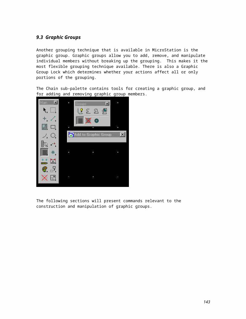
11.4 Text Placement Commands
The tools on this palette are for placing, editing, and modifying text. Several of these tools go beyond the basic 2D design concepts that are covered in this course.
Place Text - You can use this tool to place text elements in your design file or fill in empty text nodes. Depending on the placement method you select, text will be placed using some or all of the active text settings. The active element attributes: color, weight, and line style, and the active angle can affect the way your text is placed.
Place Note - This tool is used to place a line of text with a leader line and arrow as a dimension element. It is especially useful for placing geometric tolerance symbols, feature control frames, and quick notes.
Copy and Increment Text - You can use this tool to copy and increment a text element that contains numbers.
Match Text Attributes - This tool allows you to set the active text settings the same as the corresponding attributes of an existing text element.
Change Text to Active Attributes - This tool is used to change the attributes of an existing text element to the active text settings.
Place Text Node - You can use this tool to place empty text nodes that will be filled in later. The text node is placed with the active text node attributes. When text is attached to the node, it will assume these attributes. Text can be attached to a text node with the Place Text tool or by linking the node to a row in a database with the Attach Displayable Attributes tool.
Display Text Attributes - This tool allows you to see the attributes of existing text elements.
Edit Text - You can use this tool to replace, add, or delete characters from existing text elements.
Fill in Single Enter Data Field - This tool is used to fill in or change a single enter data field.
Auto Fill in Enter Data Field - You can use this tool to fill in all enter data fields in an identified view.
Copy Enter Data Field - This tool is used to copy the contents of one enter data field into another.
Copy and Increment Enter Data Field - This tool is used to copy and increment the contents of one enter data field that contains numbers into another enter data field. The numeric portion of the field is automatically increased by a tag increment.
143
11.4.1 Place Text By Origin
keyin: pla tex
The Place Text By Origin method allows text to be placed at the current active angle and active text settings. This method must be specified if you are filling text nodes.
To place a single line of text:
1. From the Text palette, select the Place Text tool. The Text Editor window will open if it is not already displayed.
2. From the Method option menu, choose the appropriate text placement method.3. In the Text Editor window, type in the desired text.4. Enter data point(s) to position the text.
The following illustration shows the placement of a single line of text using the By Origin placement method.
144
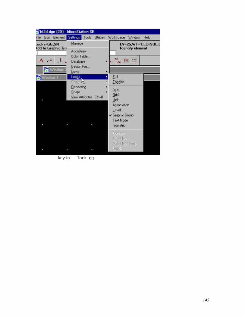
11.4.2 Place Text Fitted
keyin: pla tex fit
The fitted method allows you to force text to fit between two data points that you supply. The vertical alignment of the text element is determined by the active text justification. This method overrides the active angle and active text size settings. You can not use this method to place multi-line text.
To place fitted text:
1. From the Text palette, select the Place Text tool. The Text Editor window will open if it is not already displayed.
2. From the Method option menu, choose the fitted placement method.3. In the Text Editor window, type in the desired text.4. Enter data point 1 (Defines the beginning point of text string).5. Enter data point 2 (Defines the text size and angle of placement).
Below is an illustration using the Fitted Method.
145
11.4.3 Place Text On
keyin: pla tex on
The Place Text On an Element allows you to place a single line of text, at the active text settings, on a line or segment of a line string, shape, B-spline curve, or multi-line.
To place text on an element:
1. Select the Place Text tool. The Text Editor window opens if it is not already open.2. Set Method to On Ele(ment).3. In the Text Editor window, type the text.4. Identify the element on which to place the text. The origin of the text element is placed at this point.
The text displays. 5. Accept the text.
NOTE: The part of a line, line string, B-spline curve, or shape that is under the text is deleted.
Below is an illustration of the Place Text On Method.
146
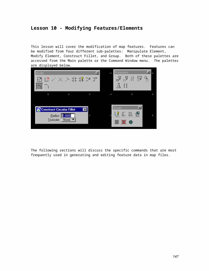
11.4.4 Place Text Above or Below
keyin: pla tex abo keyin: pla tex bel
The Place Text Above an Element method allows you to place a single line of text, at the active text settings, above a line or segment of a line string, shape, or multi-line. The active line spacing setting determines how far above the element the text will be placed.
The Place Text Below an Element method allows you to place a single line of text, at the active text settings, below a line or segment of a line string, shape, or multi-line. The active line spacing setting determines how far below the element the text will be placed.
To place a text above or below an element:
1. Select the Place Text tool. The Text Editor window opens if it is not already open.2. Set Method to Above Ele(ment) or Below Ele(ment).3. In the Text Editor window, type the text.4. Identify the line segment. The data point positions the left-to-right origin of the text element.5. Accept the text.
Below is an illustration of placing text above an element.
147
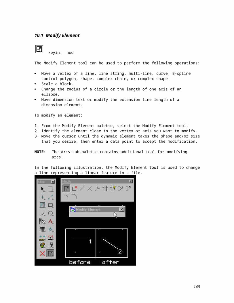
11.4.5 Place Text Along
keyin: pla tex alo
The Place Text Along an Element method allows you to place a single line of text along - above or below - a curve, arc, ellipse, line, line string, or shape. Each character that is placed becomes a single text element that is a component of a graphic group. The characters are placed at the active text settings at a distance equal to the active line spacing.
NOTE: To manipulate text placed with this method, you must have the Graphic Group lock on. This lock is located in the Locks settings box.
Below is the method for placing text along an element:
1. Select the Place Text tool. The Text Editor window opens if it is not already open.2. Set Method to Along Ele(ment).3. In the Text Editor window, type the text. See Entering and Editing Text.4. Enter a data point along the element to position the origin. The text displays both above and below the
element. If the text is too long to fit along the element with the current Interchar(acter) Spacing, it is truncated.
5. If necessary, adjust the Intercharacter Spacing.6. Enter a data point to position the text either above or below the element.
Below is an illustration of using the Place Text Along an Element method.
148
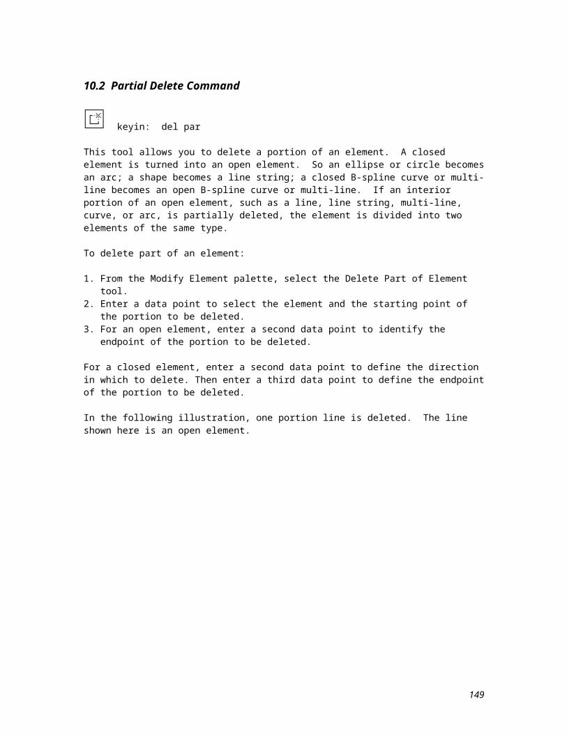
11.5 Text Nodes
keyin: pla nod
This tool is used to place empty text nodes in your design. These nodes can be filled in with text later using the Place Text tool or linked to a database row using the Attach Displayable Attributes tool. This is necessary when there is a great amount of text to be placed in addition to graphic feature data. The text node is placed with the active text attributes (text size, color, justification, weight, etc).
When text is attached to the text node, it assumes the attributes of the text node. The Text Node Lock must be on in order to attach text to the text node. The only setting associated with this tool is the View Independent check box. If this check box is on, the text appears at the same orientation regardless of the view rotation.
To place a text node:
1. From the Text sub-palette, select the Place Text Node tool.2. Enter a data point to position the text node origin and reset on the mouse to place the text node at the
active angle. Or, by placing two data points, you can define the angle of the text node. In this case, the first data point defines the location of the text node and the second sets the angle.
The following illustration shows the placement of two text nodes. Text node 3 was placed at a 0 degree angle, and node 6 at the active angle setting of 45 degrees.
NOTE: Empty text nodes are only visible in views where the Text Nodes view attribute is on. Also, you can reset the text node number with the nn= (node number) keyin.
149
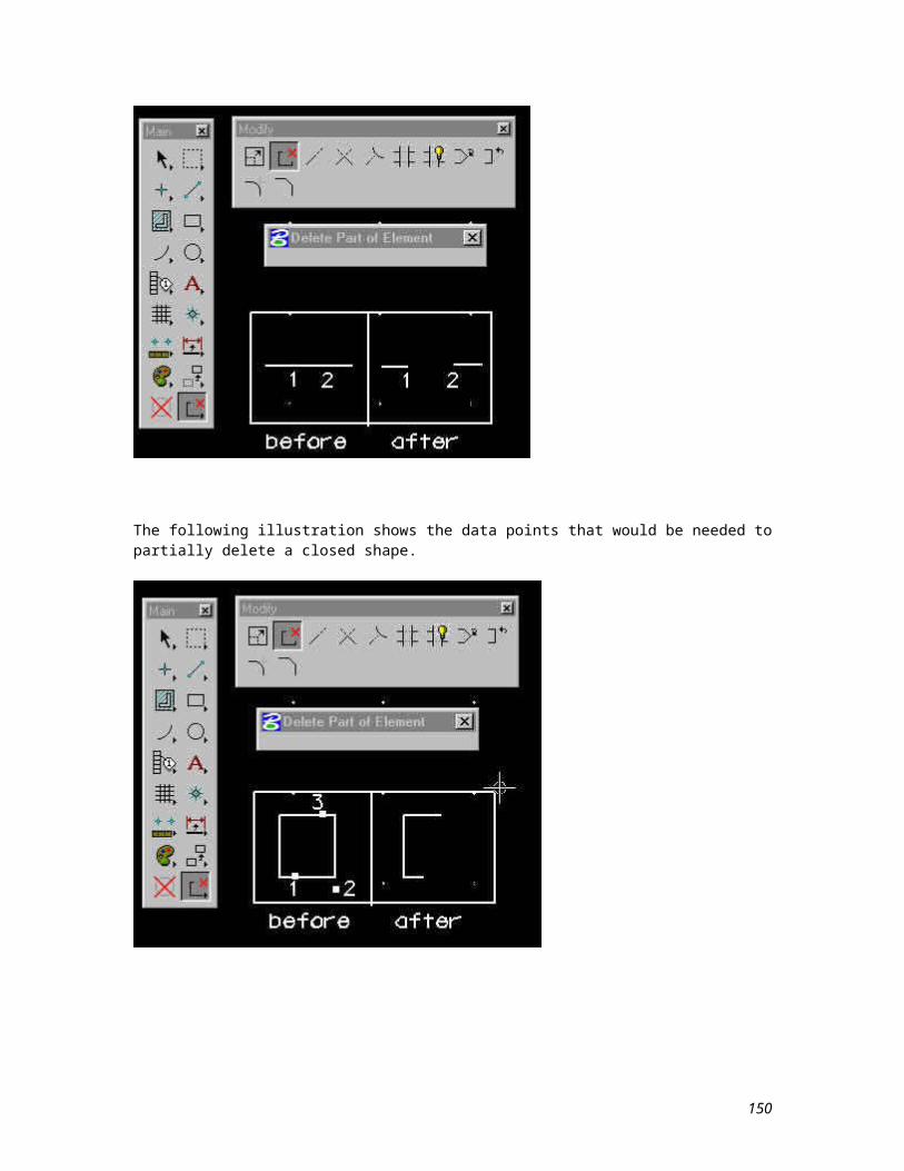
11.6 Text Manipulation Commands
The following sections will present commands that allow you to edit or change the attributes of existing text strings in a map file. Below is listed the primary functions discussed:
Edit Text Copy and Increment Text Replace Text Modify Text Match Text Display Text Attributes View Attributes for Text
150
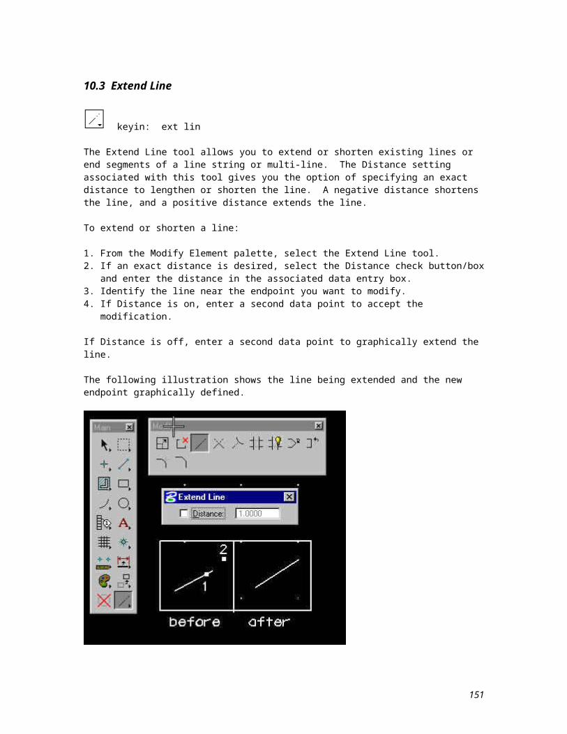
11.6.1 Edit Text
keyin: ed tex
The Edit Text tool is used to change text in existing text, text node, or dimension elements.
To edit text:
1. From the Text palette, select the Edit Text tool.2. Enter a data point to identify the text element that you want to edit.3. Enter another data point to accept the text element. The current text is now displayed in the Text
Editor window.4. In the Text Editor window, make the desired changes to the text. While in this window, you can use
the arrow keys to move the displayed cursor, a <Delete> key can be used to delete the character to the left of the cursor, a <Backspace> key to delete the character to the right. Tapping and dragging on text will highlight it and put it overstrike mode.
5. Select the Apply button to apply the changes to the text element.
In the following illustration, the Edit Text tool is used to change the words Mapping Graphics to MGF.
151
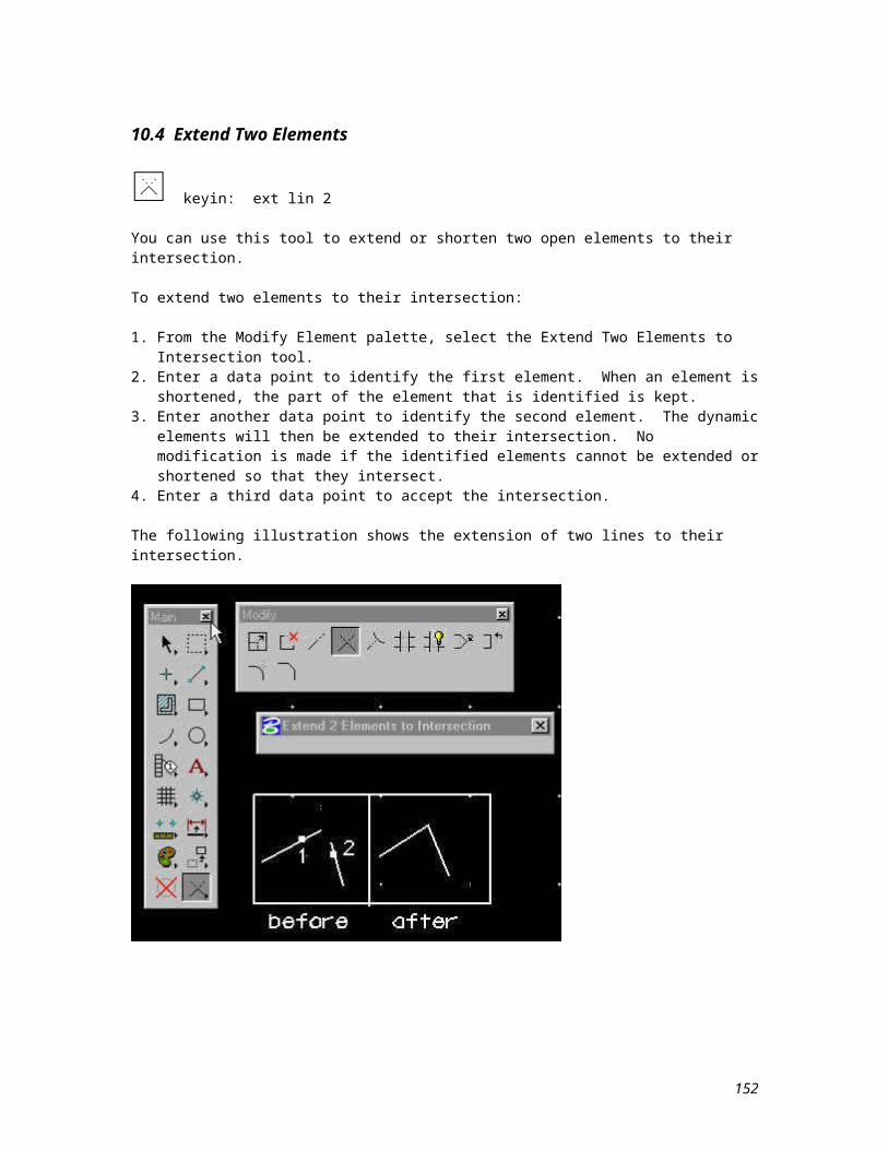
11.6.2 Copy and Increment Text
keyin: incr tex
The Copy and Increment Text tool allows you to copy and increment a text element that contains numbers.
To copy and increment text:
1. Select the Copy and Increment Text tool.2. Identify the text element to copy and increment.3. Enter a data point to position the copied and incremented text.4. Continue entering data points to place other copied and incremented text.
Below is an illustration of the Copy and Increment Text Command.
152
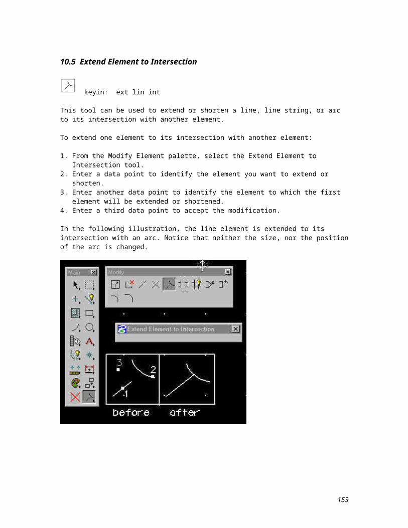
11.6.3 Replace Text
The Edit pull-down menu Replace Text item can be used to search for and replace text in your design. It displays the Replace Text settings box which allows you to search all the text in your design for any sequence of letters and numbers and replace some or all instances with other text.
The Find data entry box is where you enter the text you want to search for and the Change To data entry box is where you enter the text that you want to replace it with. The check box can be used to establish stricter match criteria. When you select the Find button, the first matching instance is displayed. You can continue selecting the Find button until the desired instance displays. At any time, you can select one of the Change buttons to change some or all of the matching instances to the Change To value.
153
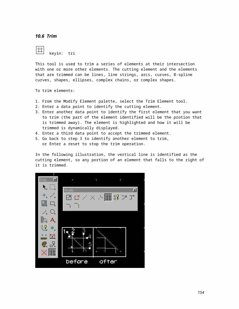
11.6.4 Change Text to Active Attributes
keyin: mod tex
You can use this tool to change the attributes of an existing text element to the current active text attribute settings. These attribute settings include font, size, justification, line spacing, and line length.
To change attributes of an existing text element:
1. If the desired text attribute settings are not currently active, use the Text settings box to change them.2. From the Text palette, select the Change Text to Active Attributes tool.3. Enter a data point to identify the text element that you want to change.4. Enter another data point to accept the element and initiate the change.
In the following illustration, the Change Text to Active Attributes tool is used to change the font and size of the word MGF.
154
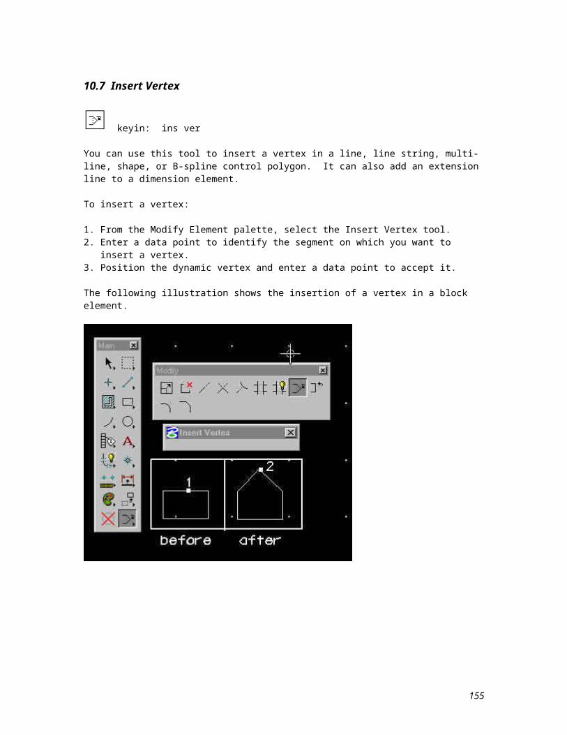
11.6.5 Match Text Attributes
keyin: mat tex
This tool is used to set the active text settings (size, justification, font, line spacing, and line length) the same as the corresponding attributes of an existing text element.
To set the active text attributes from an existing text element:
1. From the Text palette, select the Match Text Attributes tool.2. Enter a data point to identify the existing text element that has the desired attribute settings.3. Enter another data point to accept the element and initiate the settings change.
OR
1. From the Text settings box, select the Match Text button.2. Enter a data point to identify the existing text element that has the desired attribute settings.3. Enter another data point to accept the element and initiate the settings change.
155
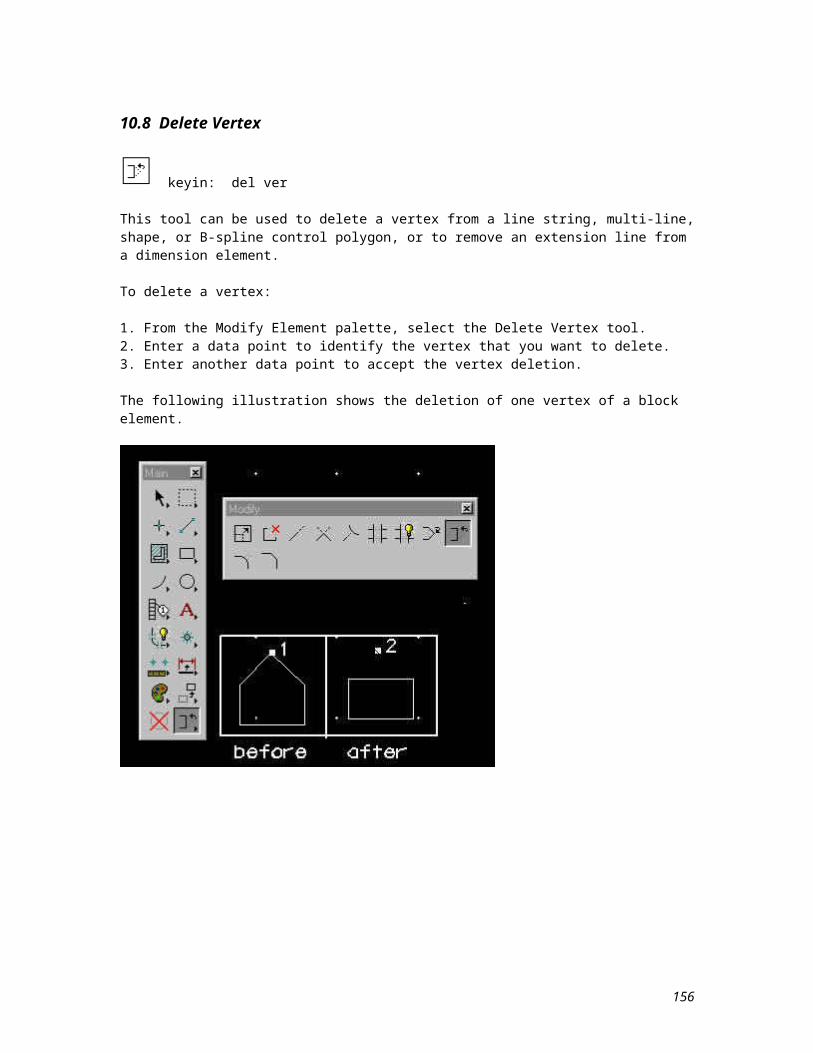
11.6.6 Display Text Attributes
keyin: iden tex
This tool will display the attributes of a text or multi-line text node element. The steps outlined below show you how to use this tool.
To display attributes of a text element:
1. From the Text palette, select the Display Text Attributes tool.2. Enter a data point to identify the text element.
If the element is a text element, the text height (TH), text width (TW), level (LV), and font number (FT) will display in the lower right corner of the Command Window.
If the element is a text node, the node number (NN), line length (LL), line spacing (LS), level (LV), and font number will display in the lower right corner of the Command Window. Entering another data point on this text node will cause the text height, text width, level, and font number to display.
The following illustration shows the use of this tool and how the information displays in the Command Window.
156
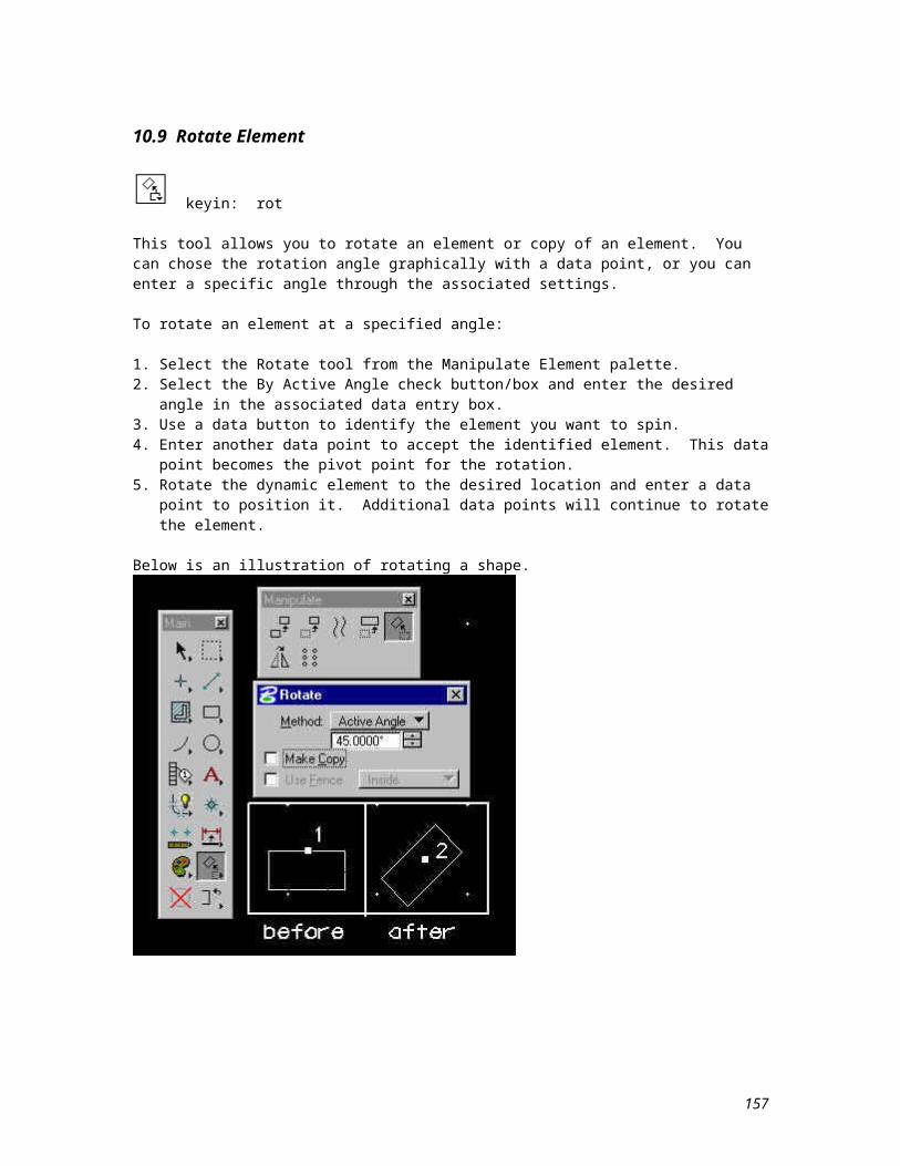
11.6.7 View Text Attributes
There are several View Attribute Settings that will impact the placement of text. Below is a listing of the parameters that should be considered when displaying text in a map file.
157
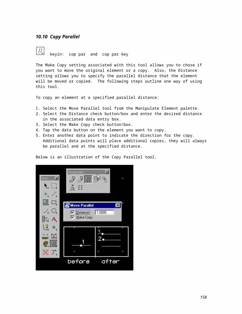
11.7 Enter Data Fields
An enter data field is a one or more character placeholder for future text input. You can insert empty enter data fields in a text element and fill in the actual text later. Enter data fields are particularly useful for variable text such as part numbers or detail numbers. Also, if enter data fields are placed in a Cell and the Cell is placed in the drawing, the enter data fields can be filled in without dropping the Cell.
To create an enter data field:
1. From the Text sub-palette, select the Place Text tool.2. In the Text Editor window, type the enter data field character (underscore by default) for every
character in the enter data field.3. Enter a data point to position the enter data field.
The following illustration shows the placement of an enter data field.
The justification for an enter data field is not the same as regular text justification. Enter data field justification can only be set with the following key-in command.
justify [ left | center | right ]
158
11.7.1 Fill in a Single Enter Data Field
keyin: ed sin
To edit an enter data field:
1. From the Text sub-palette, select the Edit Text tool.2. Identify the enter data field.3. Enter a data point to accept the text. This causes the Text Editor window to open if it is not already
open.4. Type in the text to fill in the data field, then enter.
Text in an enter data field is surrounded by delimiters (<<text>>). If there are any enter data field characters in the text, the delimiters enclose the space or spaces representing the empty placeholders. To remove an enter data field, delete the left and right delimiters. The text between the delimiters remains in the text element, but it is no longer part of an enter data field.
The following illustration shows the filling in of a single enter data field.
159
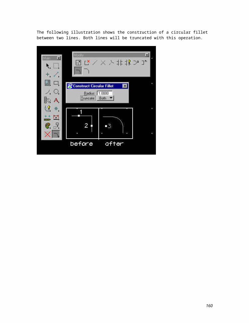
11.7.2 Fill in Multiple Enter Data Fields
keyin: ed aut
The Auto Fill in Enter Data Field tool, allows you to to fill in multiple enter data fields in an identified view. The field's justification determines the text position in the field.
To automatically fill in enter data fields:
1. From the Text sub-palette, select the Auto Fill in Enter Data Fields tool.2. Select the desired view. The first blank enter data field is located and a rectangle is displayed around
it. The Text Editor window opens if it is not already open.3. In the Text Editor window, key in the new contents for the enter data field, or enter a data point to skip
the enter data field and locate the next one.4. Press <Return> to replace the previous contents and advance to the next enter data field.5. When all fields have been filled in or skipped, go back to step 2 to fill in the enter data fields in another
view.
The following illustration shows the result of filling in of multiple enter data fields.
160
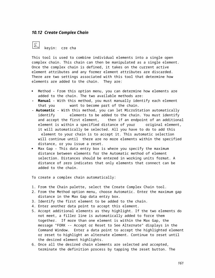
11.7.3 Copy Enter Data Fields
keyin: cop ed
The Copy Enter Data Field tool is used to copy the contents of one enter data field into another. If the source field is longer than the destination field, the copied field is truncated. The target field justification determines the text positioning within the field.
To copy an enter data field:
1. From the Text sub-palette, select the Copy Enter Data Field tool.2. Identify the source enter data field. A rectangle is displayed around the enter data field.3. Identify the destination enter data field.4. Reset to stop copying the enter data field, or return to step 3 to continue making copies of the same
enter data field.
The following illustration shows the result of copying enter data fields.
161

11.7.4 Copy and Increment Enter Data Fields
keyin: incr ed
The Copy and Increment Enter Data Field tool is used to copy and increment the contents of one enter data field that contains numbers into another enter data field. The numeric portion of the field is automatically increased by a tag increment. This tag increment is set in the data entry box that displays when this tool is selected. The value entered in this box can be any integer between 1 and 32,767.
To copy and increment an enter data field:
1. From the Text sub-palette, select the Copy and Increment Enter Data Field tool.2. Identify the enter data field to copy and increment.3. Identify the enter data field(s) in which to place the incremented copies.
The following illustration shows the copying and incrementing enter data fields.
162
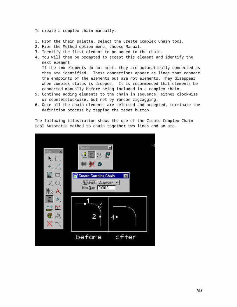
11.8 Place Note
keyin: pla not
You can use this tool to place text with a leader line. It is especially useful for strategically annotating features in extremely dense areas of a map file. This tool will allow the placement of a single-line or multi-line note in a map file.
Below are the applicable setting that will impact the Place Note tool:
Type Sets the type of text -- Single-line or Multi-line.
Font Sets the Active Font.
Text Frame Sets the type of frame (if any) -- None, Line, or Box.
Justification Controls the text alignment. · Left -- multiple lines of text are aligned along their left side · Right -- multiple lines of text are aligned along the right side · Dynamic -- multiple lines of text are aligned based on the relationship between the last and the next to last data points. For example, if the next to last data point is to the right of the last data point, the text is right justified.
Generate Leader If on, the text is placed with a leader line
Association Lock If on, snapping a tentative point to the element being dimensioned causes an association point to be created. If off, no associations are created.
To place a note:
1. From the Text palette, select the Place Note tool. This will open the Text Editor window.2. Toggle the Association Lock on or off.3. Type the desired text in the Text Editor window. If you do not enter any text, only the leader line and
arrow will be placed.4. Enter a data point to position the arrowhead.5. Enter a second data point to indicate the end of the leader line and the text.
The following illustration shows the placement of a single-line note.
163
164
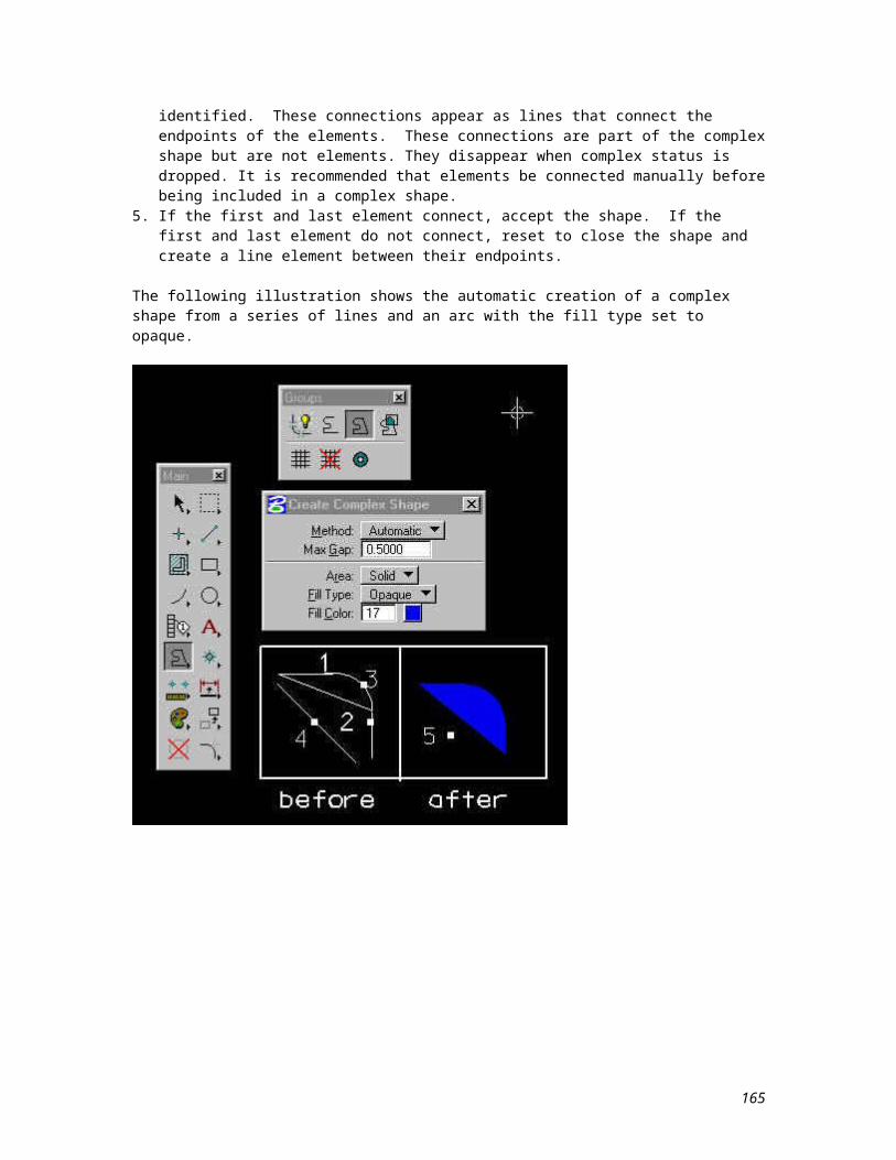
11.9 Importing a Text File
keyin: include
The Include Text File dialog box can be used to import text files into your designs. This lets you use a text editor or word processor to enter lengthy text. This dialog box is displayed by activating the File pull-down menu and selecting the Text item from Import sub-menu.
When you select the OK button, the selected text file is imported. The text displays dynamically and you must enter a data point to position it. If the file is larger than 128 lines or 2048 characters, the text is placed as a graphic group and the data point positions the upper left corner of the text block. Otherwise, the text is placed as a text node and the data point positions the text node origin.
NOTE: The imported text file can contain MicroStation key-in strings to set text attributes. Each key-in string must follow a period that begins a line, and there can only be one key-in per line. All text following a key-in string is placed with the specified attribute.
165
Lesson 12 - Cells
A cell is an element or group of elements combined into one complex element and stored in a cell library or in your design file as a shared cell. Any cell can be easily recalled and placed, and then manipulated as a single element. Cells reduce repetitive drawing and encourage standardization. With the proper setup, any cell can be used in any drawing. Therefore everyone working on a project can use the same cells if they are given access to the same cell library.
This lesson is devoted solely to cells and the tools that are used to create and manipulate them. You will learn how to create a cell library, how to create cells to put in the library, how to retrieve a cell from the cell library, and how to place a cell in your design file. The tools that are used to update and review the cell library will also be covered.
Below is the palette for cell creation and manipulation.
166
166
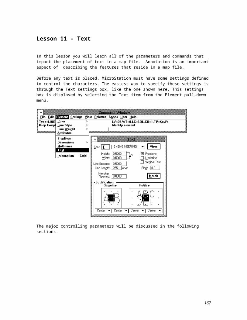
12.1 Cell Library
All cells have to be stored in and recalled from a cell library. If no cell library is available to be used with your design file, one must be created. Creating a cell library is similar to creating a design file. To create a cell library:
1. From the command window, activate the File pull-down menu and select the Cell Library item to display its associated sub-menu or from the Cell Library settings box, activate the File pull-down menu.
2. Select the New item to display the Create Cell Library dialog box shown below. 3. Enter the name of the new library in the Name data entry box. You can either specify a full path for
the file in this box, use the Directories list box to navigate to the desired directory, or use the Directory pull-down menu to access one of the last four directories. MicroStation will automatically append the standard cell library extension .cel to your filename.
4. Check the Seed File portion of this dialog box to see what seed file will be used to create the new library. If the wrong file displays, select the Seed button and choose the correct one from the associated dialog box.
5. Select the OK button to create the new cell library and dismiss the dialog box.
167
167
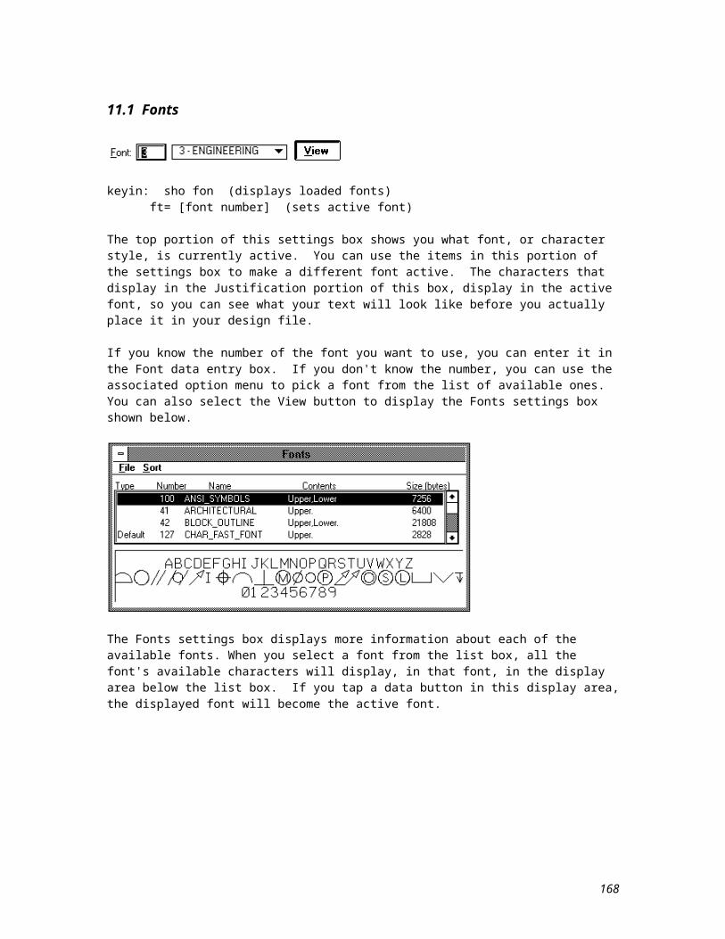
12.2 Cell Library Attachment
A MicroStation design file can have only one cell library attached at a time. But, several design files can have the same cell library attached at the same time. When you create a new cell library, that library will automatically be attached to your current design file. By default, once a cell library is attached to a design file it will remain attached until you manually detach it or attach a different one.
To attach a cell library:
1. From the Command Window, activate the File pull-down menu and select the Cell Library item to activate its sub-menu. From this sub-menu, select the Attach item to display the Attach Cell Library dialog box shown below, or from the Cell Library settings box, activate the File pull-down menu and select the Attach item.
2. Enter the name of the desired library in the Name data entry box. Use the Directories and Files list boxes to navigate through the directory structure to the desired file, or use the File and Directory pull-down menus to access one of the last four files and/or directories.
3. Select the OK button to attach the specified library and dismiss the dialog box.
keyin: rc= (cell library name)
168
168
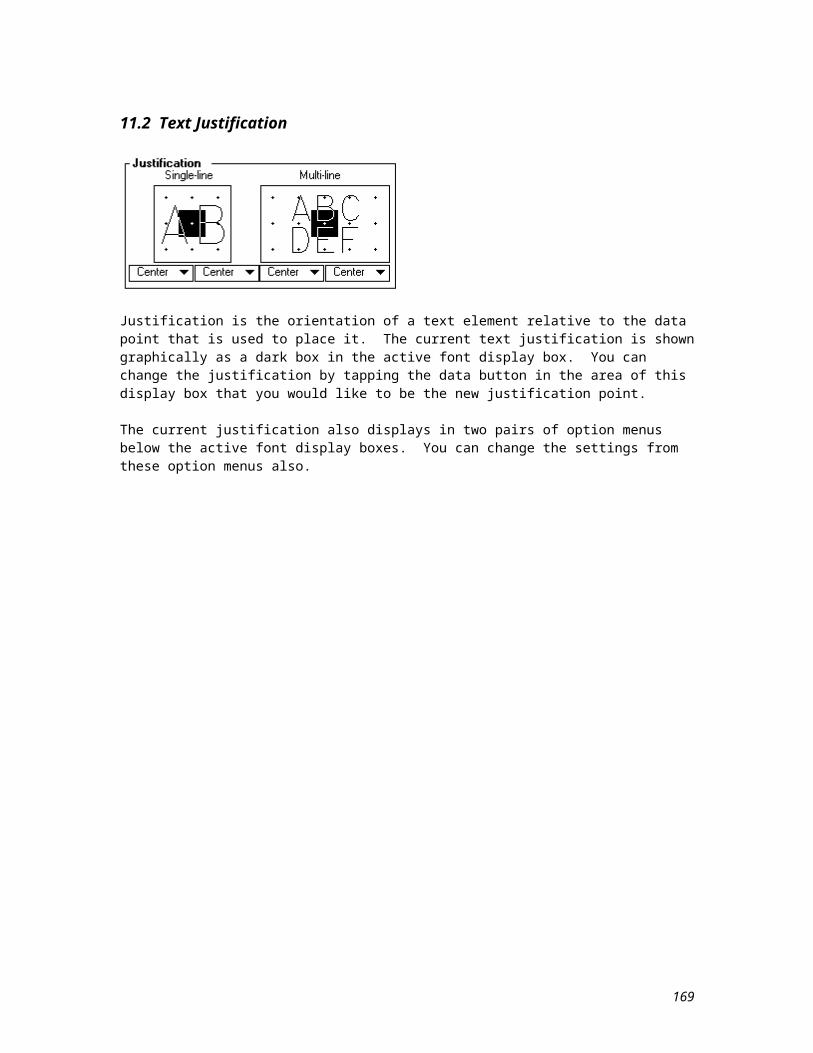
12.3 Graphic and Point Cells
There are four different types of cells that you can create in MicroStation. The following table lists the name and characteristics of each type.
Graphic: This is the default cell type. A graphic cell will retain the color, line style, and line weight for each component element as they existed when the cell was created. The destination level(s) is determined by the Relative placement setting. This type of cell rotates when a view is rotated.
Point: A point cell takes on the current active color, line style, line weight, and level for all components when it is placed. This type of cell is view independent and does not rotate when a view is rotated. Also, the only snappable point of this type of cell is the origin point.
Menu: A menu cell is used when you want to create cursor button, command, or matrix menus.
Tutorial: A tutorial cell is used when you want to create your own tutorials.
NOTE: A nested cell occurs when one or more existing cells are included in the creation of a new cell. It is even possible to nest cells inside other nested cells. It is suggested that when existing cells are to be included in the creation of a new cell, that the Drop Complex Status tool be used on all cell elements first to prevent any potential problems.
169
169
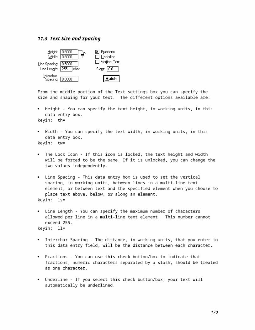
12.4 Cell Creation Process
Once you have created and attached your cell library, you can begin creating and placing cells. The following list outlines the steps necessary to create a cell.
To create a cell:
1. Create and/or attach a cell library.2. Place the elements that will be used to create the cell. Make sure that you have the desired element
attributes set when you place these elements.3. Place a fence, or use the Element Selection tool, to group the element(s) you want to include in the
cell.4. From the Cells palette, select the Define Cell Origin tool.
keyin: def cel oriDefine the origin of the cell with a data point.
5. From the Cell Library settings box, select the Create button to display the Create New Cell dialog box. Fill in the appropriate information and select the Create button to create the cell in the attached library. Through the Create New Cell dialog box, you will supply the following information:
Name: Enter the cell name in the Name data entry box. This name is limited to six characters, that can be any combination of alphanumeric, periods or underscores. Alphabetic characters can be entered in uppercase or lowercase, but MicroStation will always convert them to uppercase. Description: You can also enter an optional description in the Description data entry boxes. This description can be up to 27 characters and can include space characters. Type: Choose the desired cell type from the option menu. keyin: cc=name,description graphic cells
cc=name,description,p point cells
170
170
The following illustration shows the Create New Cell dialog box.
171
171
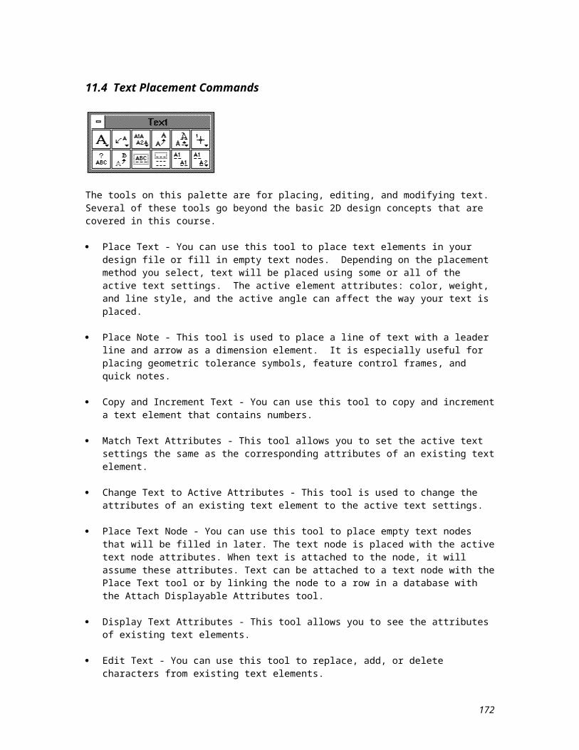
12.5 Cell Placement
keyin: pla cel
This tool is used to place the active cell. There are several settings associated with this tool that control how the cell will be placed.
These settings are:
Active Cell - You can enter the name of the cell that you want to be the active cell in this data entry box. (The active cell can also be set through the AC=).
Active Angle - If the Interactive setting is off, the cell will be rotated to the active angle. X Scale - If the Interactive setting is off, you can use this setting to scale the cell horizontally. Y Scale - If the Interactive setting is off, you can use this setting to scale the cell vertically. Z Scale - If the Interactive setting is off, this setting can be used to set the depth scale factor. (This
setting is used for 3D cells.) Relative - This settings determines the level(s) for the placement of the cell components if you want to
override the level(s) the cell was originally created on. If the active cell is a graphic cell and Relative is on, the lowest level in the cell is placed on the active
level, and the higher levels in the cell are placed relative to the active level. For example, you have a cell that was created with components on levels 10, 12, and 14. If the active level is currently level 1 and Relative is on, the cell is placed on levels 1, 3, and 5.
If the active cell is a graphic cell and Relative is off, the cell is placed on the same level(s) that the components were on when the cell was created.
This settings has no effect on point cells; they are always placed on the active level. Interactive - When this setting is on, the scale and rotation angle are defined graphically with data
points.
The following steps describe the procedure for placing the active cell in your design file. Remember, if the Use Shared Cells check button/box is on in the Cell Library settings box, the cell you place will be a shared cell.
To place the active cell:
1. From the Cells palette, select the Place Active Cell tool.2. Set the associated settings to the desired settings.3. Enter a data point to position the cell origin.
If Interactive is off, the cell is placed. If Interactive is on, you must enter two more data points. The first data point defines the scale. The second data point defines the rotation angle.
172
172
The following illustration shows the placement of the active cell, HDWAL.
173
173
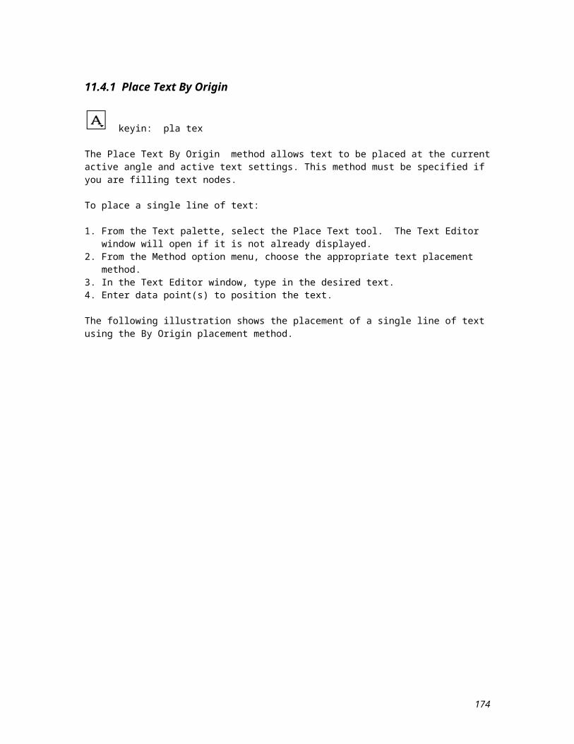
12.6 Cell Library
keyin: sho lib
Information about a cell, including a graphic depiction, can be obtained through the Cell Library settings box. The name, description, type, and location of the cells that are currently available for placement are shown in the list box.
174
174
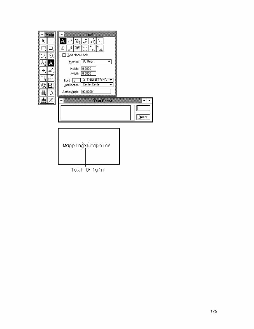
12.7 Shared Cells
Each time you place a cell in your MicroStation design file, certain information is written to the disk. This cell information can be written in one of the following two ways:
1) Unshared Cell - Each time a cell is placed, the full cell definition is written to the storage disk.2) Shared Cell - The full cell definition is only written to the storage disk one time. Any additional
instances of this cell refer to the definition that was written with the first placement. In order to use shared cells, you must select the Use Shared Cells check button/box on the Cell Library settings box. If this check button/box is on, all cells will be placed as shared cells.
Advantages and pre-cautions of using shared cells:
A much smaller file size is possible when a large number of copies of any particular cell are placed. Shared cells are not backward compatible to MicroStation Version 3.0. A modification made to the cell's definition can immediately affect all copies. Shared cells are a feature that other CAD packages may not recognize if your design file is exported to
them. A shared cell can be activated and placed using the Select and Place Cell tool, even if the cell library it
was stored in is not currently attached. A shared cell definition can not be deleted from the cell library until all instances of that shared cell are
removed.
There are two more features of shared cells that you need to be aware of. One feature allows you to place a shared cell definition in your design file without placing an instance of the cell, and the other allows you to convert a shared cell to an unshared cell.You can use the Share button on the Cell Library settings box to define the currently selected cell as a shared cell, without placing an instance of it in your design file. This could be helpful when you are customizing a seed file. The Share button will not be available if the Use Shared Cells option is off, no cell is currently selected in the list box, or the selected cell is not in the attached cell library.
To define a cell as a shared cell:
1. Open the Cell Library settings box.2. If the Use Shared Cells check button/box is not selected, select it.3. Select the desired cell from the list box.4. Tap the Share button.
175
175
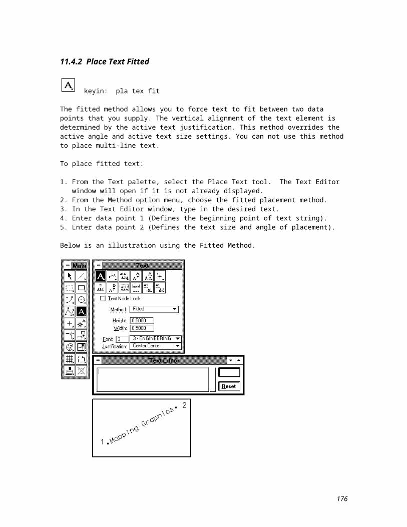
The Cell Library dialog box below displays the identification of the cell, and the parameters to be set in order to make an existing cell a shared cell.
You can also convert existing shared cell instances to unshared cells. When you do this, the full cell definition will be written for each shared cell that you convert.
To convert a shared cell to an unshared cell:
1. Type in the command drop share in the Command Window.2. Enter a data point to identify the shared cell that you want to convert.3. Enter another data point to accept the operation.
176
176
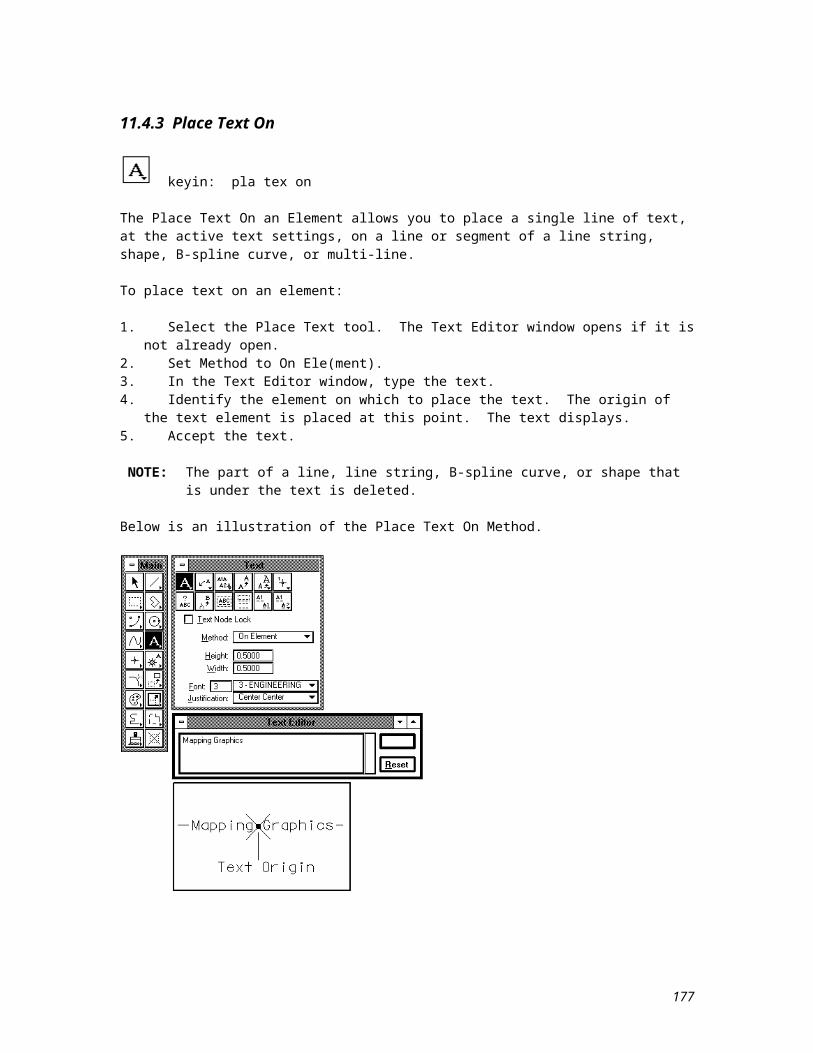
Lesson 13 - Patterning
Patterning tools are used to pattern areas and along linear elements.
The tools on this sub-palette are used to pattern areas and along linear elements. This palette is displayed by selecting the Patterning item from the Palettes pull-down menu.
Patterning tools will be discussed in the following sections.
177
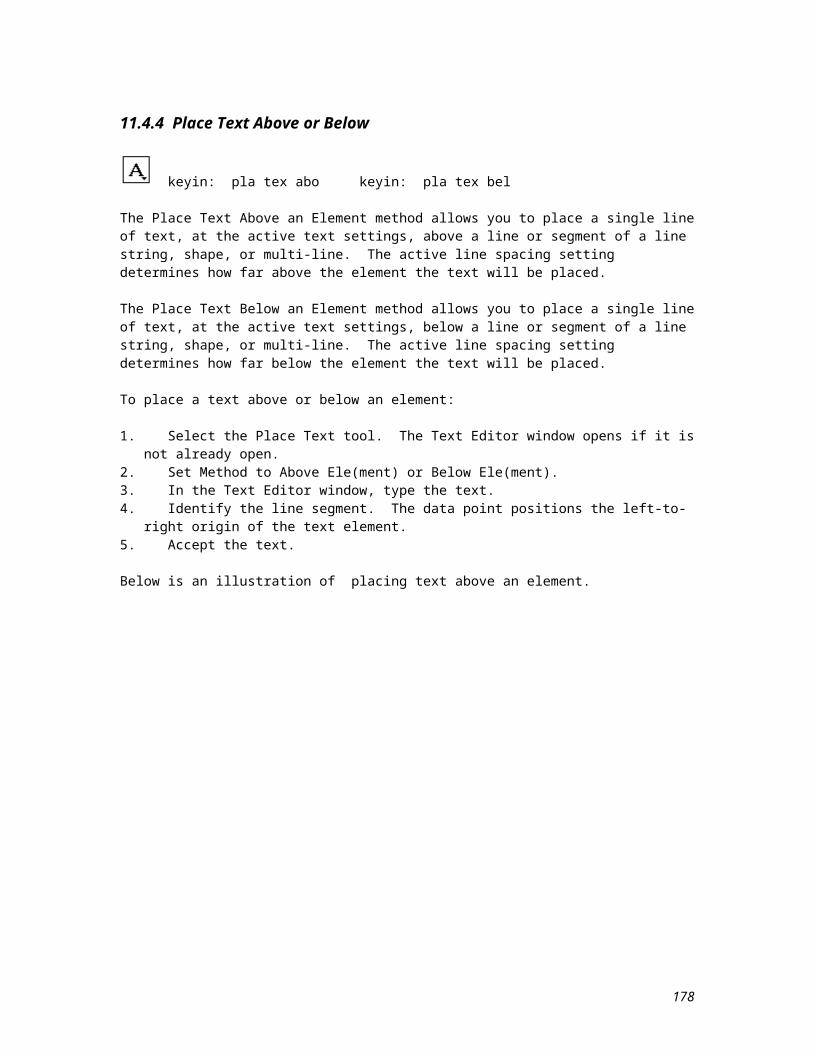
13.1 Hatch Area
keyin: hat
You can use this tool to hatch an area with lines. The various settings associated with this tool determine how the hatching will look and where it will be done. The available settings are:
Spacing - This value is the space between the hatching lines. By default, this value is set to zero. You will receive an error message in the Command Window if you do not enter some other value in this data entry box. Values should be entered in working units format.
Angle - This value sets the angle at which hatching lines will be drawn. By default, this value is also set to zero. You can enter the desired angle in this data entry box.
Tolerance - When patterning along or inside a curved element, the curve is approximated with a series of line segments that are used as guides for patterning. The tolerance is the maximum distance between the element and these line segments guides. If the tolerance is small, the line segments conform closely to the curve and the approximation is more accurate, but processing time increases. If tolerance is large, line segments do not conform closely to the curve and the approximation is less accurate, but processing time decreases.
Associative Pattern - If this check button/box is selected, hatching is associated with a patterned element and is automatically moved or resized when the element is manipulated or modified. If the patterning method is intersection, union, difference, or flood, a complex shape that bounds the patterned area is created, and the hatch lines are associated to the complex shape.
Snappable Pattern - If this check button/box is selected, you will be able to snap to the elements in the pattern.
Method - This setting determines the area that will be hatched. The items available on this option menu are:Element - The interior of a shape, ellipse, or closed B-spline curve, or between the components of a multi-line will be patterned.Fence - The area inside the fence will be patterned.Intersection - The intersection of two or more closed elements will be patterned.Union - The union of two or more closed elements will be patterned.Difference - The difference between two or more closed elements will be patterned.Flood - The minimum area enclosed by a set of elements will be patterned.Points - An area defined by a series of data points will be patterned. Each specified data point defines a vertex.Max Gap - This is the maximum distance, in working units, between the endpoints of enclosing elements when the Method is set to Flood.
178
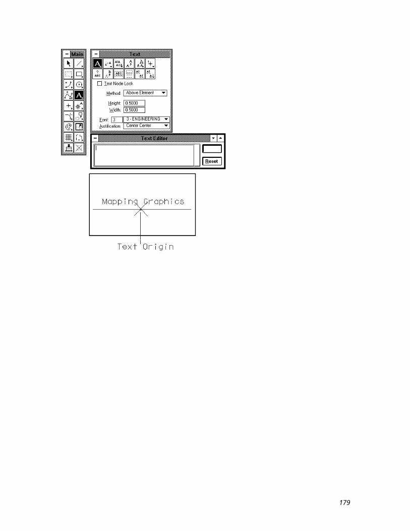
To hatch an area using the Element, Fence or Flood method :
1. From the Patterning palette, select the Hatch Area tool.2. In the tool settings area for this tool, set all the desired settings.3. Enter a data point to identify the element you wish to hatch. If the Method is Fence, this data point is
not necessary. For the Flood method, enter a data point inside the closed area to be flooded.4. Enter another data point to define a point through which a hatch line must pass.
The following illustration shows the Element method of hatching. Notice that the Spacing value was set to a value other than zero and that the Angle was set to 45 degrees. Since the Associative Pattern check box is on, the hatching will automatically update if the shape is modified.
179
13.2 Cross Hatch
keyin: crosshat
This tool is very similar to the Hatch Area tool. The tool settings and the procedures are the same, except that there are two additional data entry boxes to specify the spacing and angle of the crosshatch lines. There are two ways that you can use the Spacing and Angle boxes for the crosshatch lines:
You can enter the desired angle and/or spacing, in working units, in the appropriate data entry box. You can leave either value set to zero. If the spacing is zero, the crosshatch lines will have the same
spacing as the hatch lines. If the angle is zero, MicroStation will automatically calculate an angle for you. This angle will be 90 degrees from the angle that you specified for the hatch lines. For example, if you leave both Angle values set to zero, the hatch lines will be at 0 degree angles and the crosshatch lines will be at 90 degree angles.
The following illustration shows the crosshatching of an shape.
180
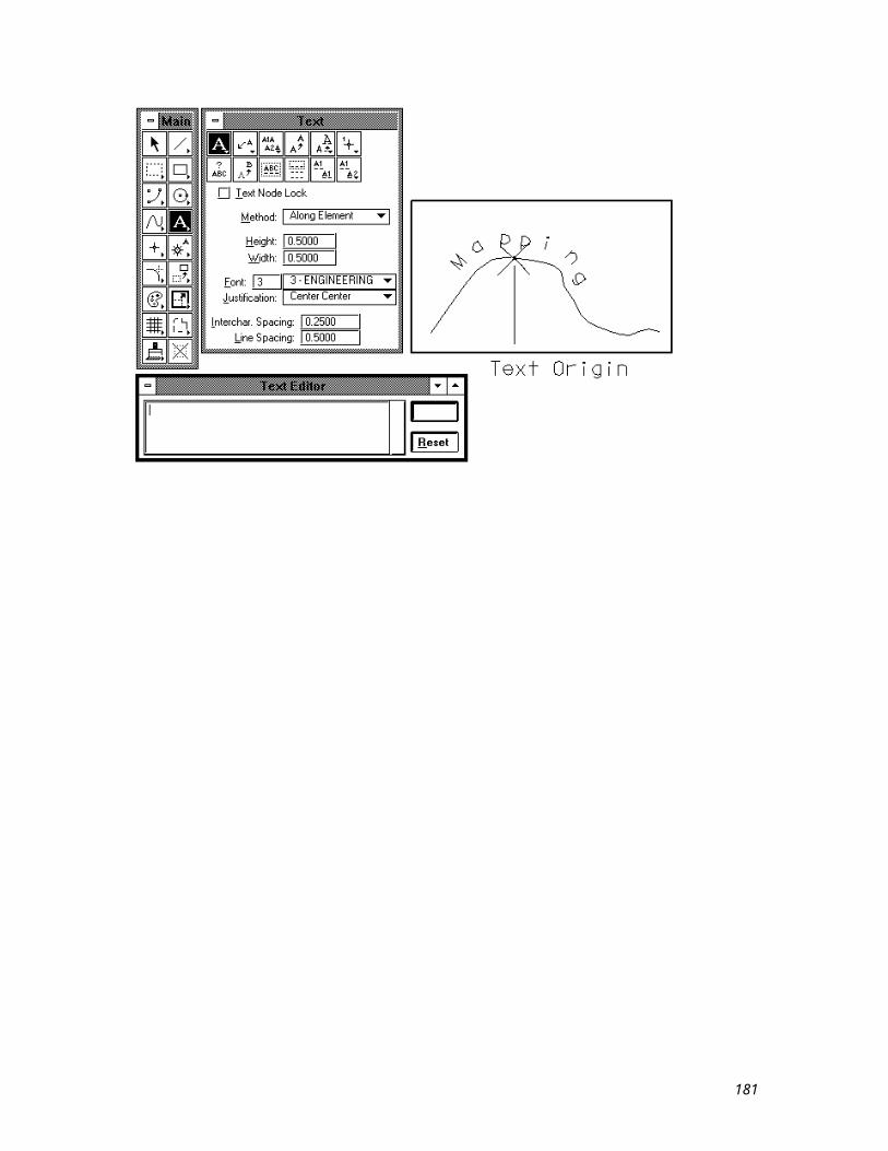
13.3 Area Patterning
keyin: pat are
The Pattern Area tool is used to pattern an area by tiling instances of the active Pattern cell. There are several settings associated with this tool that determine what cell is used, how it will be spaced, and what area will be patterned. These settings are:
Pattern Cell - The cell name that appears in this data entry box is the cell that will be used to create the pattern. You can select another cell by entering a different cell name in this box, or by using the Pattern button on the Cell Library settings box.
Scale - This data entry box is used to set the scaling factor for the pattern cell. Row Spacing - You can specify the desired spacing between rows in this data entry box. Column Spacing - You can specify the desired spacing between columns in this date entry box. Angle - The angle specified in this data entry box is the angle at which instances of the pattern cell are
placed. Tolerance - This value is the maximum distance between a curved element and the line segment guides
used for patterning. Associative Pattern - This check button/box determines whether or not patterning will automatically
adjust if the patterned element is modified. Snappable Pattern - This check button/box determines whether you can snap to the individual pattern
elements. Method - You can specify the area that is patterned through this option menu. The individual items are
described with the Hatch Area tool. Max Gap - This value sets the maximum distance between the endpoints of enclosing elements when
the Method is set to Flood.
To pattern an area using the Element, Fence, or Flood method:
1. From the Patterning palette, select the Pattern Area tool.2. In the tool settings area for this tool, set all the desired settings.3. For the Element method, enter a data point to identify the element.
For the Flood method, enter a data point inside the area enclosed by the set of elements. For the Fence method, skip this step.
4. Enter a data point to place the origin of one of the pattern cells.
NOTE: A cell library must be attached to use this command
181
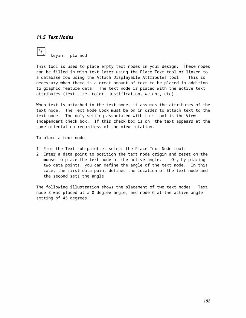
In the following illustration, the Element method is used to pattern the shape with the HDWAL cell.
182
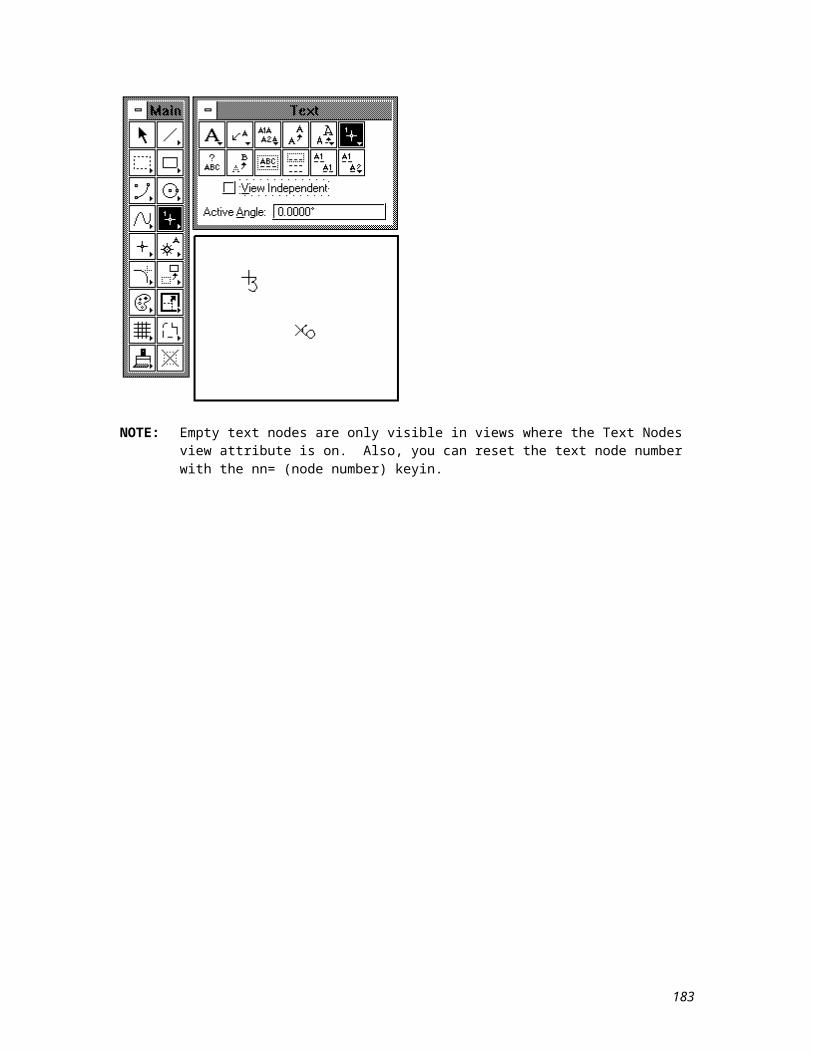
13.4 Linear Patterning
keyin: pat lin
The Linear Pattern tool is used to draw a pattern along a linear element. There are several settings associated with this tool that affect how the patterning is placed. These settings are:
Cycle - The items in this option menu determine how the active pattern cell is placed. The available items are:
Single - One instance of the pattern cell is placed on each segment. A segment is a line, arc, curve, or ellipse; or each segment of a line string, shape, complex chain, or complex shape. If a segment's length is less than 80% of the cycle length, the segment is patterned with the first horizontal line in the pattern cell.
Multiple - The pattern cell is placed along an element at a scale that is adjusted, if necessary, from the active pattern scale so that every instance is complete along each segment. If a segment's length is less than 80% of the cycle length, the segment is patterned with the first horizontal line in the pattern cell.
Truncated - The pattern cell is placed along the element at the active pattern scale. If necessary, the last instance is truncated.
Complete - The pattern cell is placed along the element at a scale that is adjusted, if necessary, from the active pattern scale so that only complete instances are placed.
Pattern Cell - The cell name that appears in this data entry box is the cell that will be used to create the pattern. You can select another cell by entering a different cell name in this box, or by using the Pattern button on the Cell Library settings box.
Scale - This data entry box is used to set the scaling factor for the active pattern cell. Tolerance - This value is the maximum distance between a curved element and the line segment guides
used for patterning.
NOTE: This type of patterning is supported to maintain compatibility with existing applications and for customers who have existing designs with linear patterns. In most cases, however, defining a custom line style is far more efficient, and is recommended for new design work.
183
To pattern along a linear element:
1. From the Patterning palette, select the Linear Pattern tool.2. In the tool settings area, set the desired settings.3. Enter a data point to identify the element.4. Enter another data point to indicate the desired pattern direction.
NOTE: A cell library must be attached to use this command.
Below is an illustration.
184
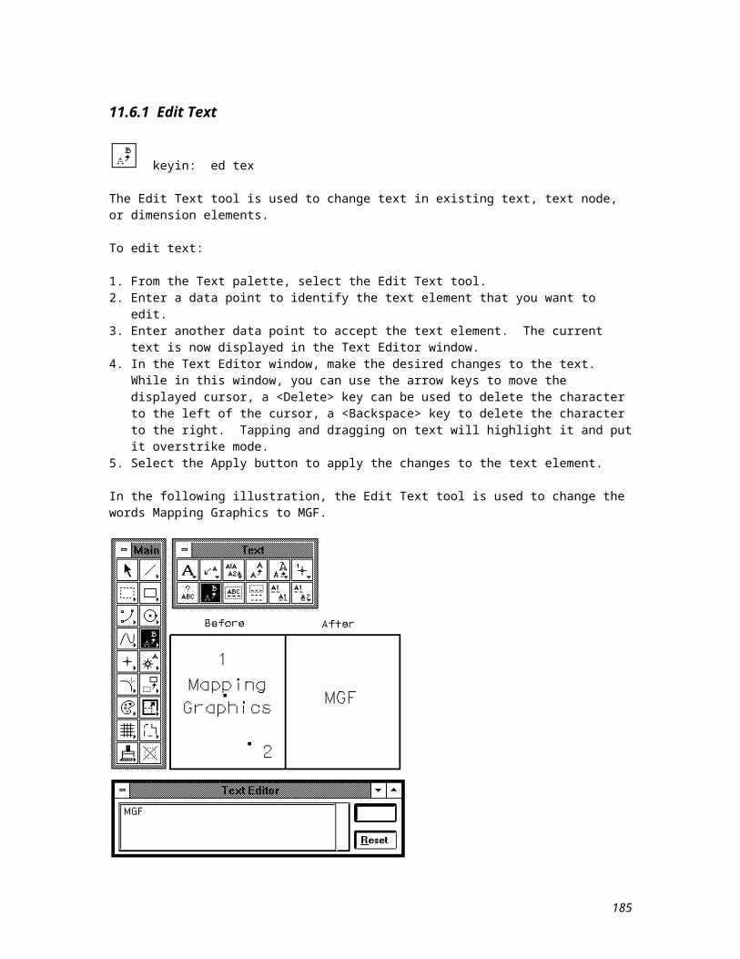
13.5 Show Pattern Attributes
keyin:
You can use this tool to display the angle and scale attributes of a pattern element.
To show pattern attributes:
1. From the Patterning palette, select the Show Pattern Attributes tool.2. Enter a data point to identify the pattern element. The type and level information for the highlighted
pattern element displays in the Command Window.3. Enter another data point to accept the pattern element. The angle and scale display in the Command
Window.
The following illustration shows the type of information that displays in the Command Window, after the pattern has been accepted.
185
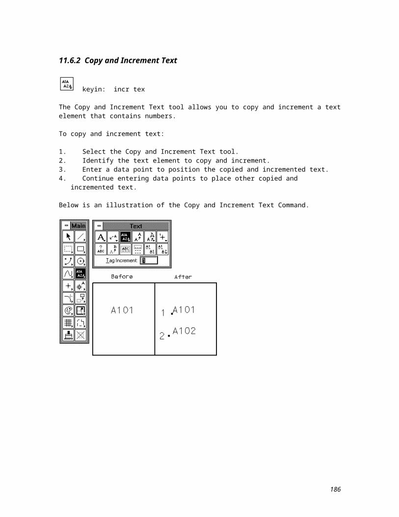
13.6 Delete Pattern
keyin:
Most patterning operations can be undone with the Undo item from the Edit pull-down menu. But some patterning operations can be so complex that they will exceed the capacity of the undo buffer. This means that the only way to undo the patterning is to delete it. The Delete Pattern tool provides a quick and easy way to do this.
To delete patterning:
1. From the Patterning palette, select the Delete Pattern tool.2. Enter a data point to identify the patterning that you want to delete.3. Enter another data point to accept it.
186
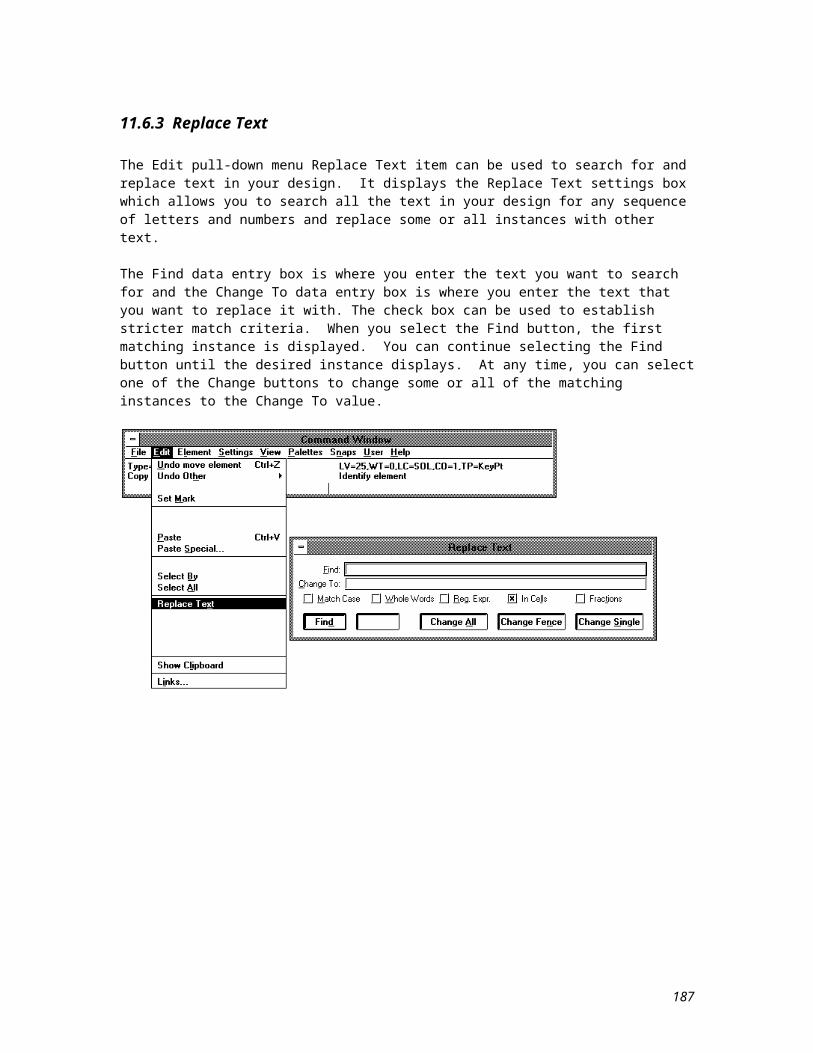
13.7 Pattern View Attributes
The display of pattern elements is turned on and off through the Patterns settings in the View Attributes settings box.
187
13.8 Custom Linestyles
Along with the seven default line styles, there are also custom line styles that you can use. Custom line styles includes line styles that you create, and the custom ones that are automatically delivered with MicroStation.
To activate a custom line style:
1. From the Element pull-down menu, select the Line Style item to display its associated sub-menu.2. From the sub-menu, select the Custom item to display the Line Styles settings box.3. From the list of available line styles, double tap on the one that you wish to activate.
188
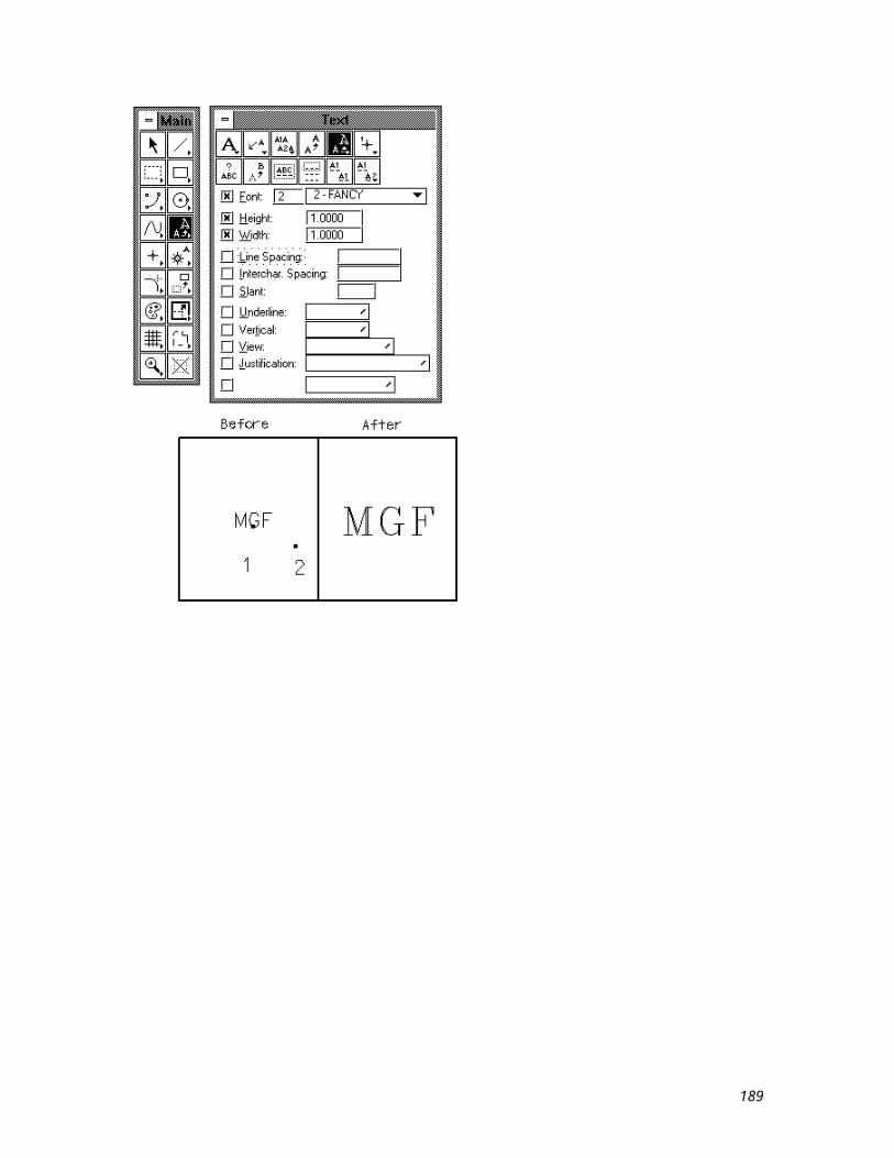
If you wish to see more information about a line style, such as a sample, select the Show Details check box. This will display the expanded Line Styles settings box, like the one shown below.
To edit a linestyle you would click the Edit option just below the Custom option and the following setting box will display.
189
Lesson 14 - Measurements
There are several different methods available in MicroStation for measuring elements. Some are useful for measuring length and distance, while others measure area and volume. This lesson introduces the six measuring tools that are found on the Measuring sub-palette.
When you complete this lesson, you should be able to:
Measure the distance between points, along elements, or between elements. Measure the radius of an element. Measure the angle between two lines. Measure the length of an element. Measure the area and perimeter of an element.
190
14.1 Measure Distance Tool
keyins: meas dist poi | meas dist alo | meas dist per | meas dist min
The Distance option menu associated with this tool allows you to specify how you want to measure distances. The choices you have are:
Between points - This option will measure the distance between data points. This measurement is cumulative.
Along element - You can measure and display the distance along an element with this option. This will be a cumulative measurement along one element.
Perpendicular - This option will measure the perpendicular distance between an existing element and a specified data point.
Minimum between - This option will measure the minimum distance between two existing elements.
To measure the distance between points:
1. From the Measuring palette select the Measure Distance tool.2. From the Distance option menu, choose the Between Points item.3. Enter a data button to identify the first point.4. Enter another data point to identify the second point. The distance between these points will display in
the Command Window. Additional data points will continue to total the segments being measured.
191
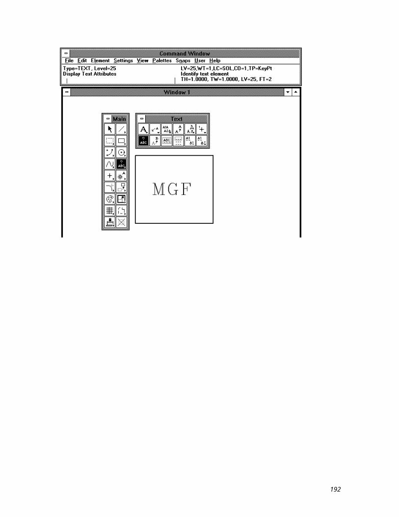
In the following illustration, seven data points were entered to measure the distance around this odd shaped element. The measurement shown in the Command Window is the cumulative distance from data point 1 to data point 6.
192
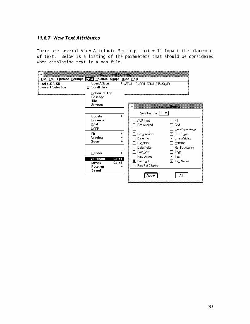
14.2 Measure Radius
keyin: meas rad
The Measure Radius tool allows you to measure the radius of a circle, circular arc, cone, or cylinder, or the axis of an ellipse or elliptical arc. When you activate this tool, you will be prompted to identify the element that you want to measure. Tap the data button on the element, tap another data button to accept the element, and the radius measurement will appear in the Message field of the Command Window.
To measure the radius of an element:
1. From the Measuring palette select the Measure Radius tool.2. Enter a data button to Identify the Element.3. Enter a data button to Accept, Initiate the measurement.
Below is an illustration.
193
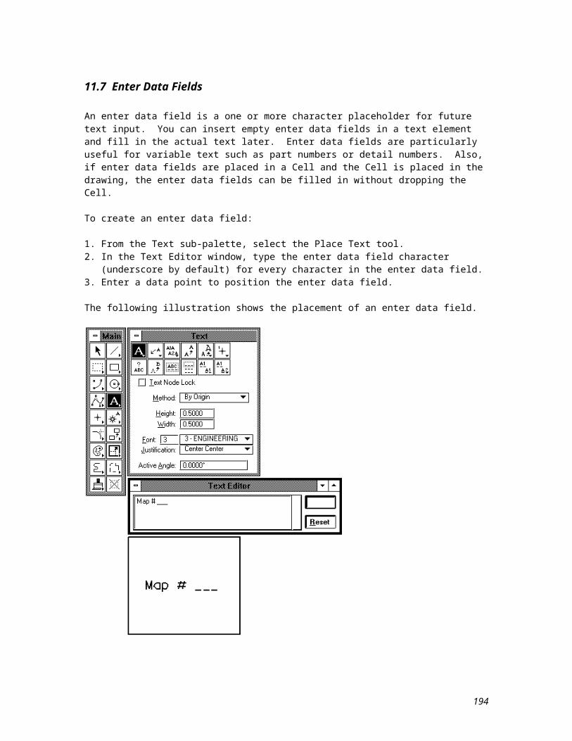
14.3 Measure Length
keyin: meas len
The Measure Length tool will measure the length of an element, and will analyze mass properties.
To measure the length of an element:
1. From the Measuring palette select the Measure Length tool.2. Enter a data button to Identify the Element.3. Enter a data button to Accept, Initiate the measurement.
Below is an illustration.
194

14.4 Measure Area
keyin: meas are
The Measure Area tool is used to measure the area of closed elements. This tool displays both the surface area and the perimeter measurement for the selected element. The settings for this tool are:
Tolerance (%) - You can use this data entry box to specify the maximum percentage of the distance between the true curve and the approximation used when measuring curves. A low tolerance makes the measurement more accurate, but increases calculation time.
Mass Properties - If this settings is on, the Mass Properties window displays the mass properties analysis.
Display Centroid - If this setting is on, the graphic crosshair that represents the center of mass for the measured element is displayed.
Method - You can select the area that is measured from this option menu. The available menu items are:Element: Measures the area of one closed element. Its Area attribute must be Solid.Fence: Measures the area enclosed by the fence.Intersection: Measures the area bounded by the intersection of two or more closed planar elements.Union: Measures the area bounded by the union of two or more closed planar elements.Difference: Measures the area bounded by the difference of two or more closed planar elements.Flood: Measures the area enclosed by elements that either touch each other or whose endpoints fall within the Max Gap value.Points: Measures the area defined by a series of data points.
Max Gap - The value entered in this data entry box sets the largest distance allowed between consecutive elements, if the Method is Flood. If this value is zero, the elements must connect to bound an area.
To measure the perimeter and area of one element:
1. From the Measuring palette, select the Measure Area tool.2. Set the Method setting to Element, and set any other desired tool settings.3. Enter a data button to identify the element you want to measure.4. Enter another data button to accept the element and the measurements display in the Command
Window.
195
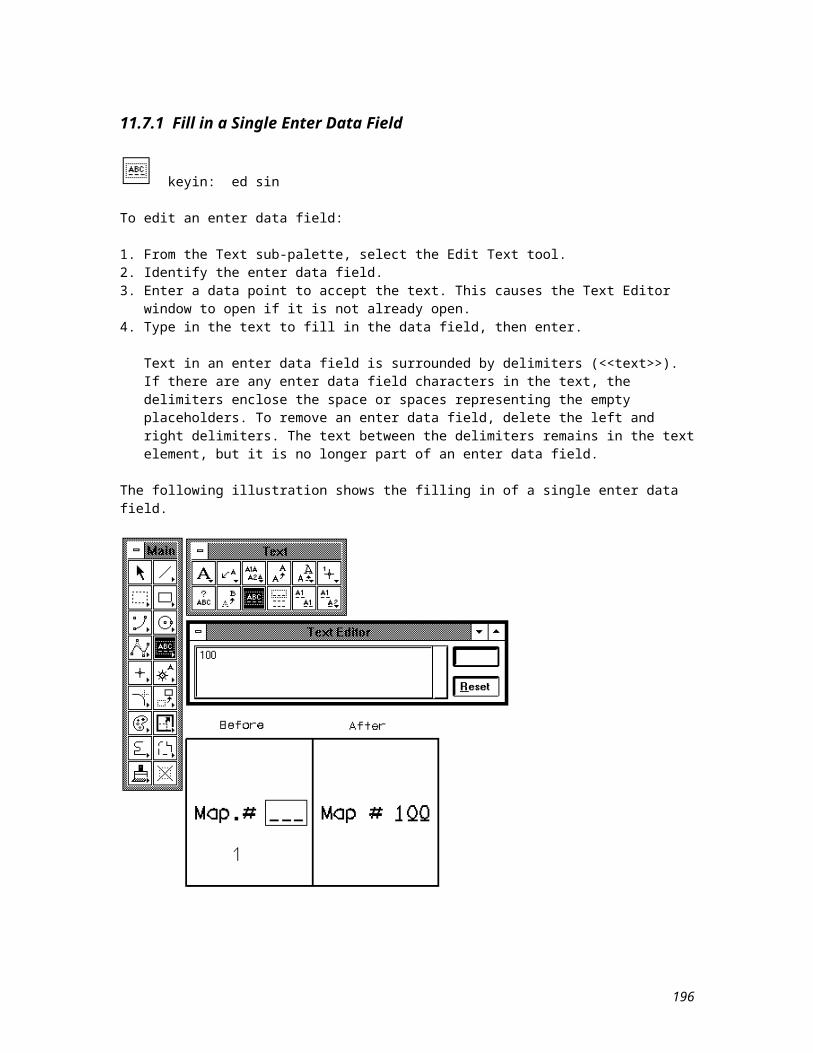
In the following illustration, the area and perimeter of the selected shape are displayed in the Command Window.
196
Lesson 15 - File Manipulations and Saved Views
In this lesson you will gain exposure to several file manipulation utilities. These utilities will allow you to copy or move the contents of one map file to another, and also exit a map file and go directly into another without accessing the Microstation Manager interface. The concept of saved views will also be discussed.
197
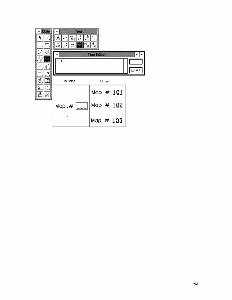
15.1 File Manipulations
In this section several file manipulation utilities will be discussed. Among these are the Fence File, Separate Fence, and Retrieve Design tools.
198
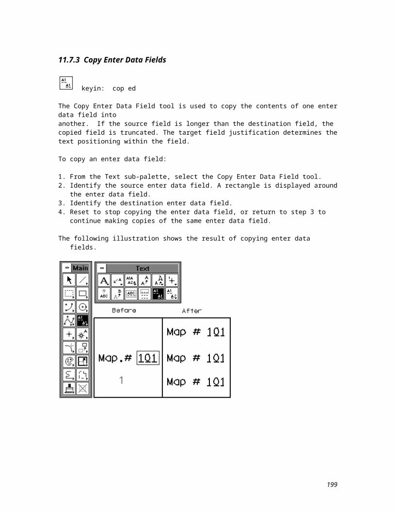
15.1.1 Copy the Fence Contents to a New Design File
keyin: ff=
This utility will copy the contents of a fence from the current map file you are accessing to a destination map file. This utility will either create a new file or overwrite an existing map file.
The two methods for performing this function are listed below:
1. Place a fence around the elements to be copied and set the fence lock to the appropriate setting (inside, overlap, clip, ...).
2. In the Key-in window, key in FENCE FILE or FF=. The Save Fence Contents As dialog box opens.3. Key in the name of the new file and set the directory in which to create it.4. Click the OK button.5. Accept the copy,
or
1. In the Key-in window, key in FENCE FILE <filename> or FF=<filename>.2. Accept the copy.
The file is created in the directory that is pointed to by the MS_DEF configuration variable.
199
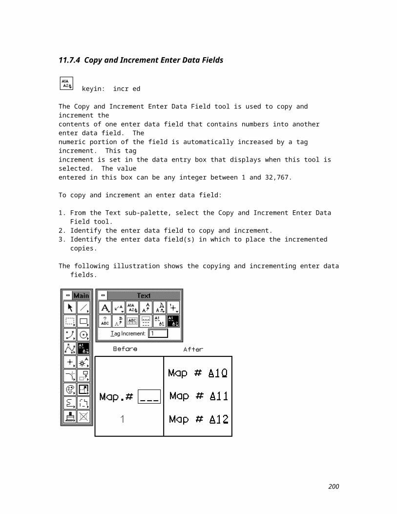
Below is an illustration of using the first method with the Fence Clip lock on.
NOTE: When using the second method, if a file already exists with the specified filename, an alert box warns you that it will be overwritten.
200
15.1.2 Move the Fence Contents to a New Design File
keyin: sf=
This utility will move the contents of a fence from the current map file you are accessing to a destination map file. This utility will either create a new file or overwrite an existing map file.
1. Place a fence around the elements to be moved and set the fence lock to the appropriate setting (inside, overlap, clip, ...).
2. In the Key-in window, key in FENCE SEPARATE or SF=. The Save Fence Contents As dialog box opens.
3. Key in the name of the new file and set the directory in which to create it.4. Click the OK button.5. Accept the move.
or
1. In the Key-in window, key in FENCE SEPARATE <filename> or SF=<filename>.2. Accept the move.
The file is created in the directory that is pointed to by the MS_DEF configuration variable.
201
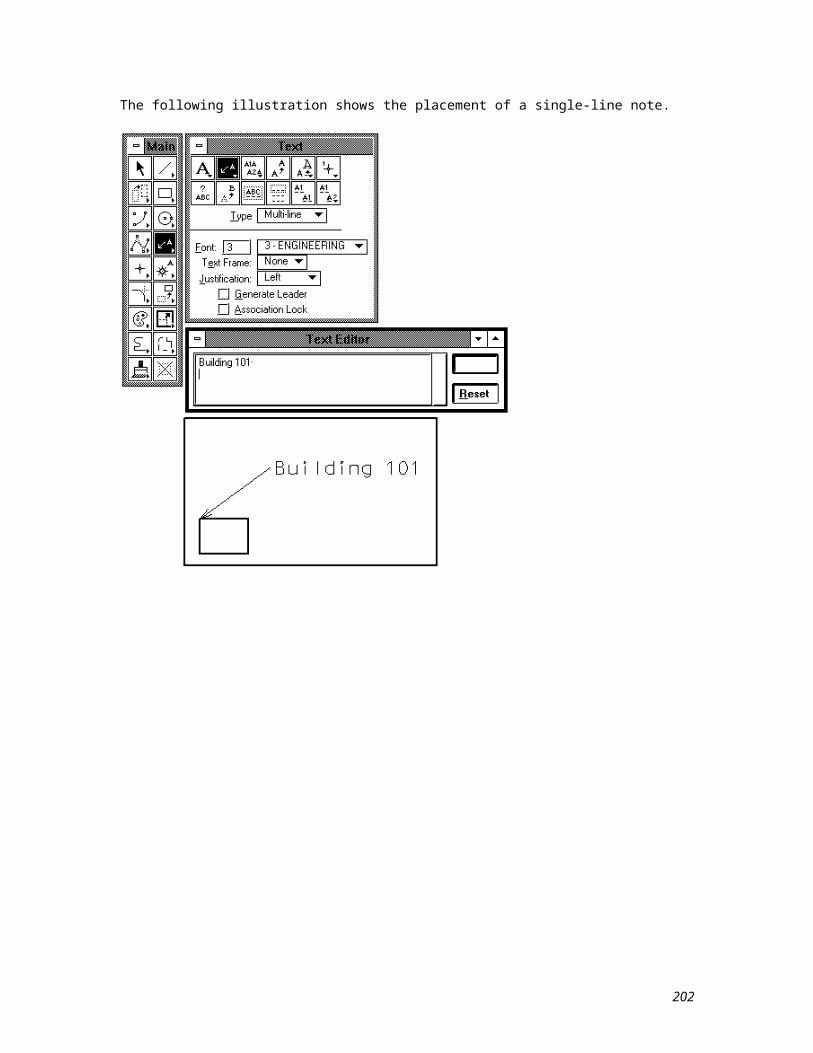
Below is an illustration of using the first method with the Fence Clip lock on.
NOTE: When using the second method, if a file already exists with the specified filename, an alert box warns you that it will be overwritten.
202
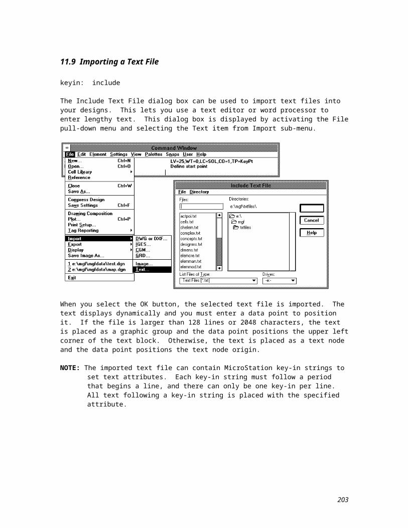
15.1.3 New File and Exchange Files
keyins: New file, rd= (file name)Exchange files, xd= (file name)
Using the NEWFILE (RD=) key-in can be faster than using the Open Design File dialog box to open a design file. The syntax is RD=<design_file> or NEWFILE <design_file>.
You can open a design file with the view configuration of the active design file by keying in one of the following:
EXCHANGEFILE <filename>EXCHANGEFILE UPDATE <filename>EXCHANGEFILE NOUPDATE <filename>
This is a convenient way to make a reference file the active design file for modification. The alternate key-in is XD=.
203
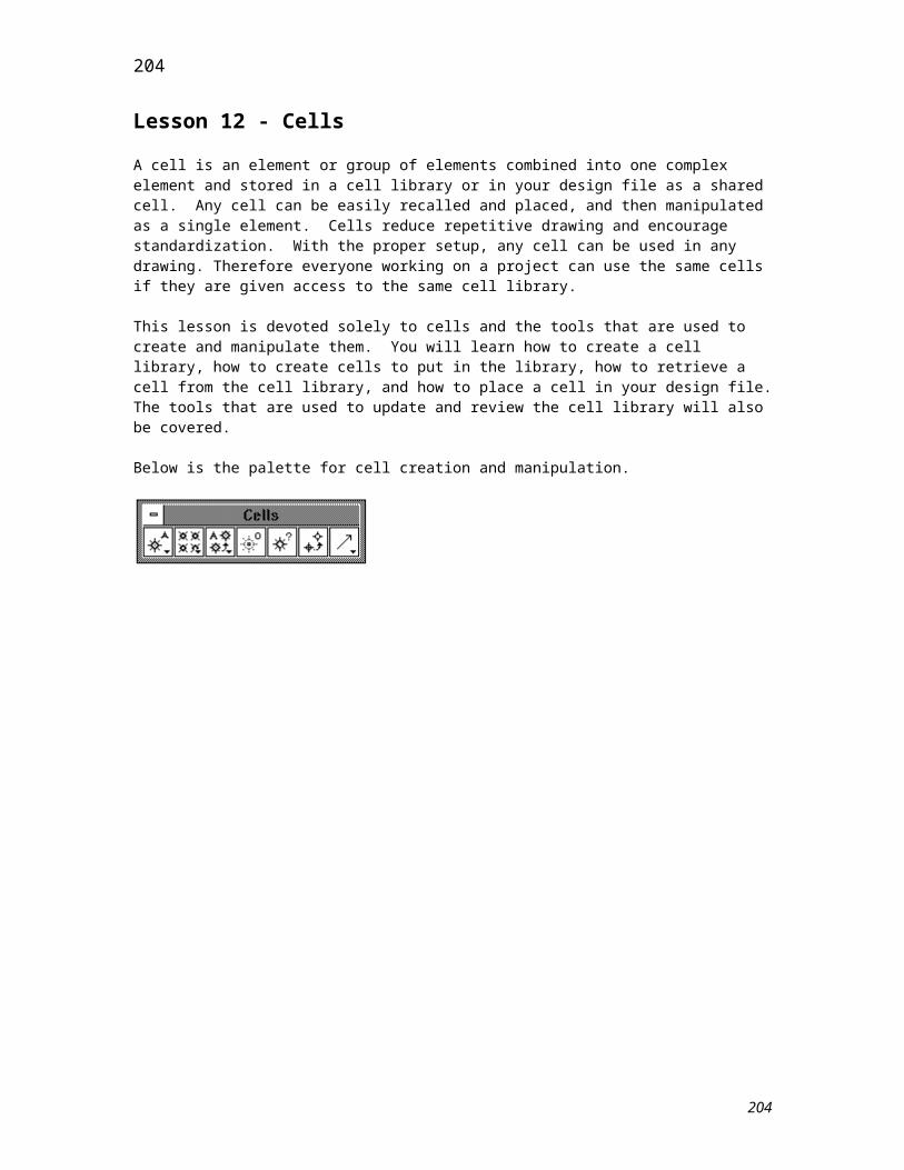
15.2 Saved Views
Once you have a view set up the way you want it, you may want to save its settings so you can easily recall them later. You can do this by creating a saved view. A saved view is a view definition that is given a name and saved in the design file. You create the definition by setting up a source view as a model and saving it. The saved view can be recalled and attached to a destination view so that the destination view has the same attributes and displays the same portion of the design as the source view.
For example, if you are producing a road map for a state you would have the entire state conveyed on the map. You would have as blown-up insets on the map the largest metropolitan areas. This would provide you with much greater detail for these areas. These blown-up insets could be saved views either from the map file of the entire state or from another file that contains detailed information about the respective metropolitan area.
Saved views can be created and recalled through the Saved Views settings box. This settings box is displayed by activating View pull-down menu and selecting the Saved item. The Source portion of this settings box is where you can specify the information for the view you want to save. The Saved portion is where you can attach these saved view settings to other views.
204
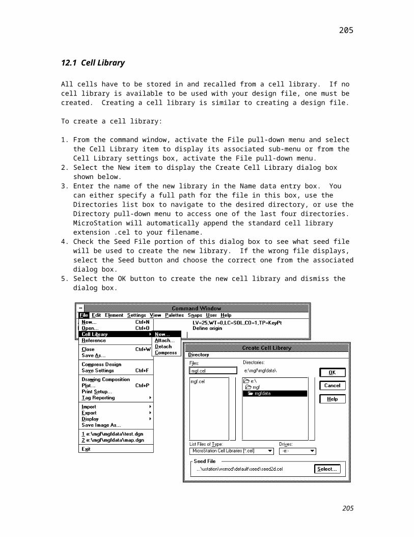
15.2.1 Naming/Saving a View
keyin: sv= (name of the view)
To save a view:
1. Set up the source view so that the desired view orientation and attributes are displayed.2. From the View pull-down menu, choose the Saved item.3. From the View option menu, select the number of the source view.4. Enter a name for the saved view in the Name data entry box. This name can include up to six
alphanumeric characters (no case sensitivity), the underscore, dot, space, or dollar sign characters.5. You can enter an optional description of the view in the Description data entry field. This description
can be a maximum of 27 characters (same character set as the Name field).6. Select the Save button to create the saved view.
205
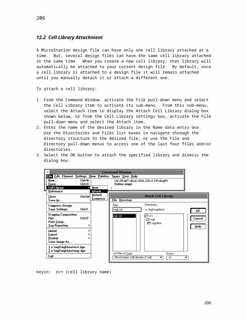
15.2.2 Recalling a Named View
keyin: vi= (name of the saved view)
To attach a saved view:
1. From the View pull-down menu, select the Saved item.2. From the Dest View option menu, choose the number of the destination view.3. Select the saved view that you want to attach from the list box.4. Select the Attach button.
206
15.2.3 Deleting a Named View
keyin: dv= (name of the saved view)
To delete a saved view:
1. From the View pull-down menu, select the Saved item.2. From the list box, select the saved view that you want to delete.3. Select the Delete button.
207
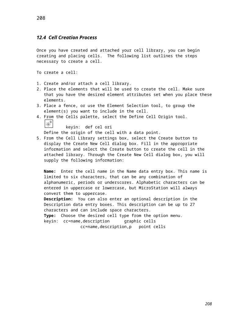
Lesson 16 - Reference Files
Reference files are other design files, either local or remote, that are attached or associated with the active design file. You can display the elements in the reference file as though they were in the active design. This allows you to use them for reference and construction purposes, and even plot them along with the active design. Although you can not manipulate the elements in a reference file, you can snap to them and even copy them into the active design file. MicroStation even allows you to attach the active design file as a reference file to itself. This allows you to reference one part of the design while drawing in another area.
Each time you load a design file that has attached reference files, those files will be loaded too, as long as MicroStation has access to the directory path in which they are stored. MicroStation will allocate enough RAM memory to load at least 16 reference files. The default setting reserves memory space for 32 files on most systems. There is a user preference setting that, depending on your hardware configuration, may permit up to 255 maximum reference files to be attached to one active design.
208
208
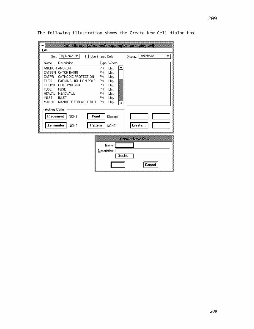
16.1 Reference File Interface Mechanisms
There are two basic interfaces that allow you to work with reference files: The Reference File Settings Box and the Reference Files Palette. These will be discussed below.
The Reference File Settings Box
From the File pull-down menu, select the Reference File item to display the Reference Files settings box. This settings box may be used to attach reference files, review the list of reference files currently attached, adjust the attachment settings, and manipulate reference files.
The following illustration shows this settings box with no reference files attached.
The Reference Files Palette
The tools on this palette are used to attach reference files to the active design file, control the positioning, scaling, and orientation of attached reference files, and detach reference files. This palette is displayed by activating the Palettes pull-down menu and selecting the Reference Files item.
209
209
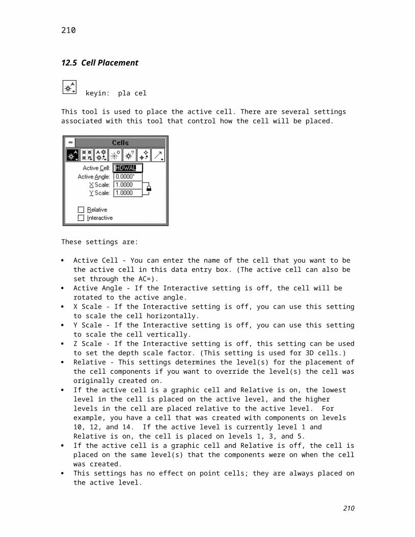
The following illustration demonstrates how to activate the Reference Files Palette.
210
210
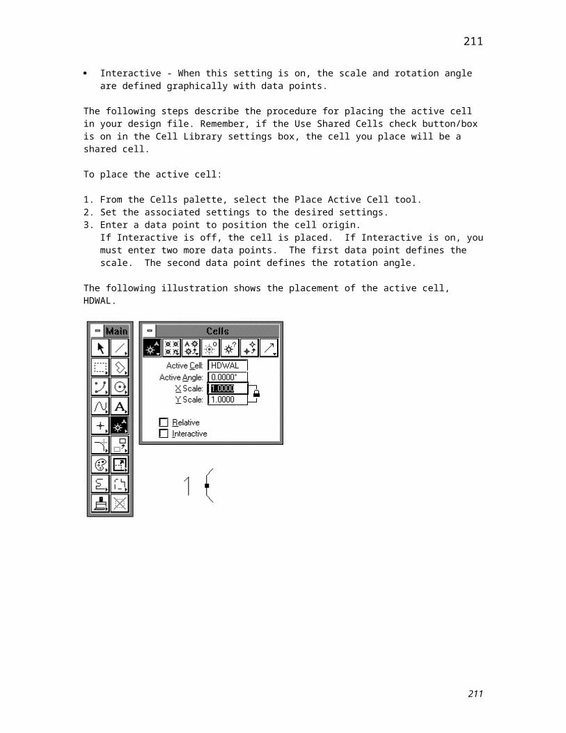
16.2 Reference File Attachment
keyin: ref att
This tool is used to attach a reference file to the active design file.
To attach a reference file:
1. Select the Attach Reference File tool to display the Attach Reference File dialog box.
211
211
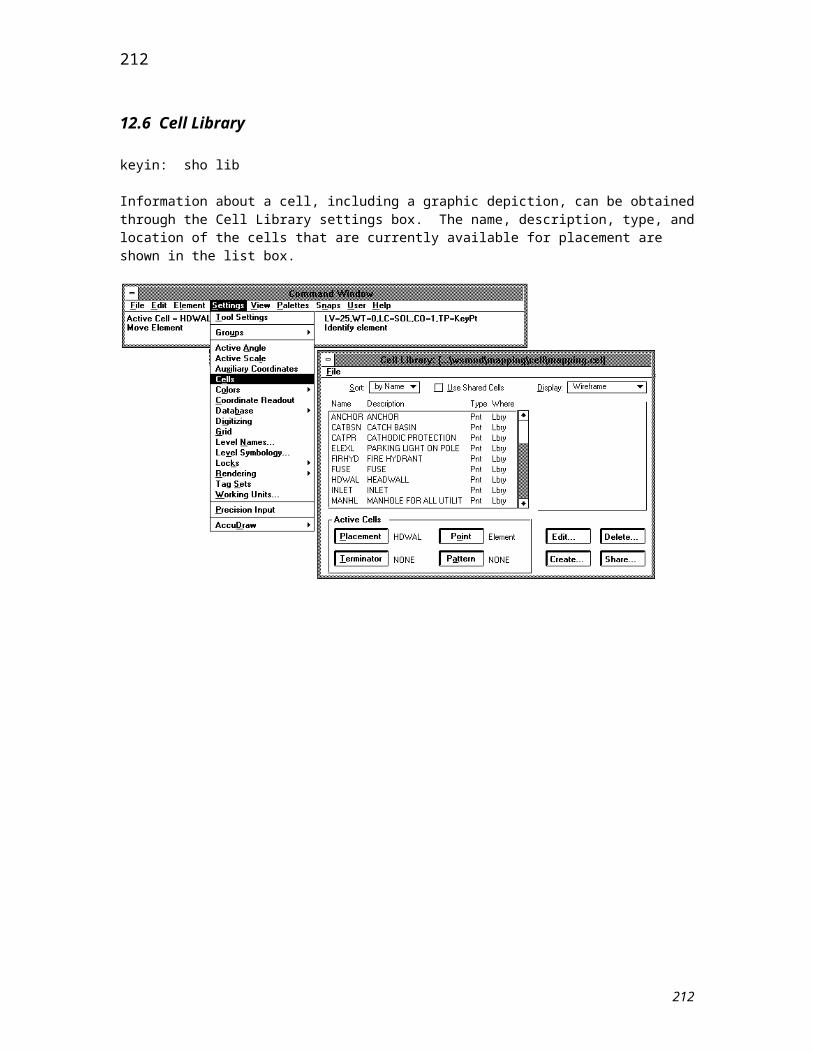
2. From the Attach Reference File dialog box, select the reference file for attachment and choose the OK button. This will display another dialog box, like the one shown below.
3. In the Logical Name data entry box, you may enter up to 20 characters that will be used as the logical name for the attached reference file. This is not necessary if this is the first attachment of this file, but it is necessary on subsequent attachments of the same file. Logical names make it easier to identify reference files and transfer design files to different computer systems that are running MicroStation.
4. In the Description data entry box, you may enter up to 40 characters that will be a description for the attached reference file. This is not required.
5. From the Attachment Mode option menu, select the desired attachment mode. The valid choices are:Coincident: This mode specifies that the reference file will have the same coordinates as the active design file.Saved View: This mode specifies that you want to attach one of the reference file saved views that display in the list box. You should select the desired saved view from the list box and the mode will highlight automatically. The Scale data entry boxes define the ratio of design file master units to reference file master units.
6. Select the Scale Line Styles check button/box if you want to scale user defined line styles.7. Select the OK button to attach the file. If the Saved View mode is used, enter a data point to position
the center of the reference file view.
212
212
Below is an illustration of an attached reference file in the Reference File Setting box.
There are several attachment settings that you can specify for any attached reference file. To set these settings, activate the Settings pull-down menu and select the Attachment item.
From this settings box, you can specify the following information:
Logical Name - A logical name for the reference file can be entered in this data entry field. Description - A description for the reference file can be entered in this data entry field. Display - An attached file can be made invisible by turning off this setting and then updating any of the
eight views. Snap - Using a tentative point to snap to reference file elements will only be permitted when this
setting is enabled. Locate - This option will allow you to use the Copy Element tool to import reference file elements,
making the copied objects part of your active design file; unless an element is part of the active file, it cannot be modified in any way.
213
213

16.3 Identifying a Reference File
Except for the Attach Reference File tool, reference file tools operate on the reference file that is selected in the Reference Files settings box. If no reference file is selected, you must identify one. There are three basic ways that a reference file can be identified:
Select the reference file in the Reference Files settings box. Identify an element in the reference file. Enter the reference file's name or logical name in the Command Window.
214
214
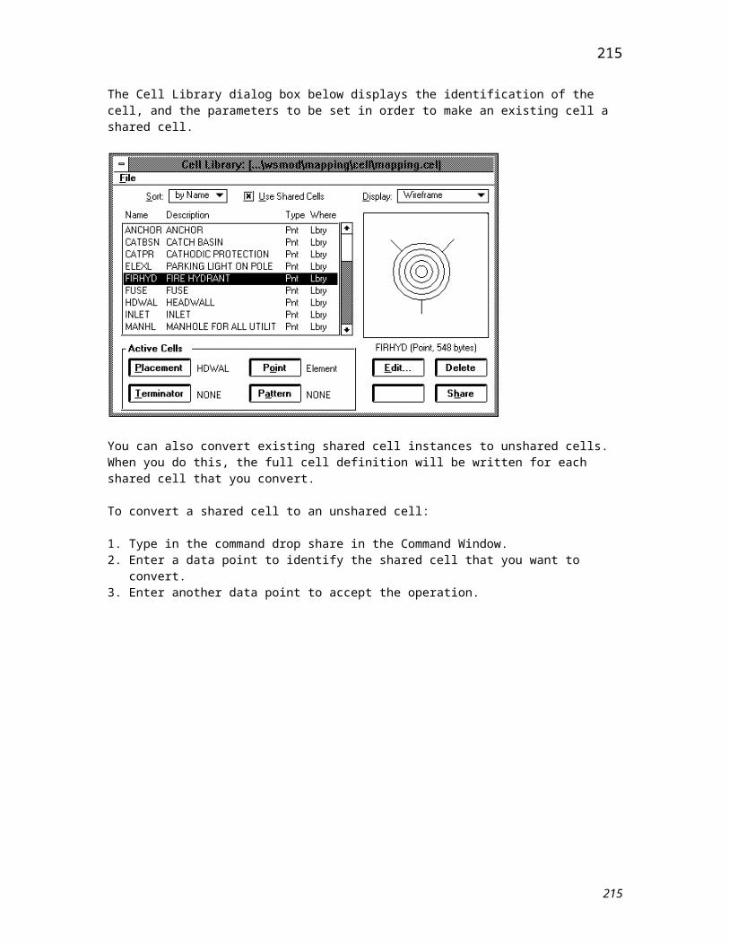
16.4 Reference File Level Display
You can turn on or off the level display for attached reference files just like you can for your design file. When you select the Levels item from the Settings pull-down the Reference Levels settings box will display. From this settings box, you can control the level display for the reference file that is highlighted in the Reference Files settings box.
keyin: ref lev on | ref lev of
215
215
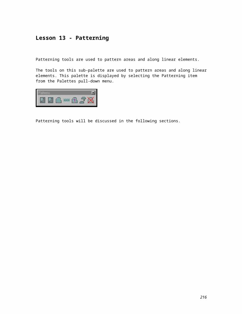
16.5 Reload Reference File
keyin: ref rel
The Reload Reference File tool is used to reread and redraw a reference file. This will display changes that may have been made to the file since it was last attached or reloaded.
To reload a reference file:
1. Select the Reload Reference File tool.2. If necessary, identify the reference file. The reference file is read from disk and redrawn.
216
216
16.6 Move Reference File
keyin: ref mov
This tool is used to change the position of the reference file data with respect to the active file data. This tool does not move the elements in the reference file, but rather changes the relationship between the reference file's origin and the active file's origin.
To move a reference file:
1. Select the Move Reference File tool.2. If necessary, identify the reference file.3. Enter a data point to define the origin of the move.4. Enter a data point to define the destination.
217
217

16.7 Scale Reference File
keyin: ref sca
You can use this tool to change the scale of an attached reference file. This command does not scale the data in the reference file, but changes the relationship between the reference file's master units and the active file's master units. This scale factor may be set in the tool settings area associated with this tool or in the Scale Reference File dialog box. This is an absolute scale.
To scale a reference file:
1. Select the Scale Reference File tool.2. Enter the desired scale value in the Scale data entry boxes.3. If necessary, identify the reference file.4. Enter a data point to scale around.
218
218
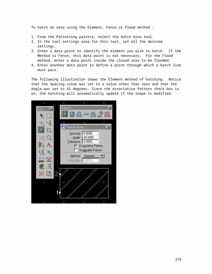
16.8 Rotate Reference File
keyin: ref rot
This tool is used to change the orientation of an attached reference file. This command does not rotate the elements in the reference file; it changes the relationship between the axis of the reference file and those of the active file. The angle of rotation can be specified in the tool settings are associated with this tool or in the Rotate Reference File dialog box.
To rotate a reference file:
1. Select the Rotate Reference File tool. 2. Enter the desired rotation angle.3. If necessary, identify the reference file.4. Enter a data point to define the pivot point.
NOTE: It may not be possible to a rotate a whole reference file unless the Reference Clip Boundary tool is used, or the reference file was attached using a saved view.
219
219
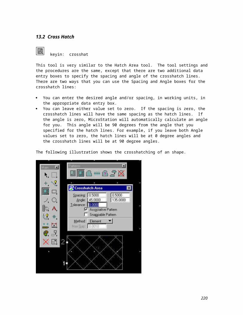
16.9 Reference File Clip Boundary
keyin: ref cli bou
You can use this tool to redefine the outer limit (boundary) to be displayed for an attached reference file. A fence is placed to indicate the desired boundary. Any reference file elements outside the fence will no longer be visible.
To define a reference file clipping boundary:
1. Place a fence to define the reference file clipping boundary's position.2. Select the Define Reference File Clipping Boundary tool.3. If necessary, identify the reference file. The reference file elements, or any portion of an element,
outside the fence will disappear.
There are two view attributes that affect how clipped reference files are displayed. They are:
Reference File Boundaries - If this attribute is on, reference file clipping boundaries are displayed in the view as a dashed line.
Fast Reference File Clipping - This attribute determines whether non-rectangular clipping boundaries are displayed.
- If this attribute is on, all attached reference files are clipped to rectangular boundaries, which are orthogonal to the view and the enclosed boundary points.- If this attribute is off, the reference file is displayed and plotted as specified by a non-rectangular clipping boundary.
NOTE: These view attributes are set through the View Attributes settings box. This box is displayed by activating the Command Window Views pull-down menu and selecting the Attributes item.
220
220
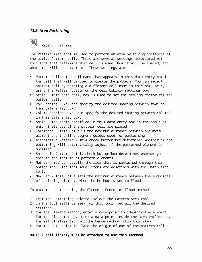
16.10 Reference File Clip Mask
keyin: ref cli mas
Used to place a reference file clipping mask that covers part of a reference file that is inside the clipping boundary. More than one clipping mask can be specified for a reference file. Reference file elements display only if they are inside the clipping boundary and outside all clipping masks.
To place a reference file clipping mask:
1. To define the reference file clipping mask's position, place a fence with the Place Fence tool.2. Select the Define Reference File Clipping Mask tool.3. Identify the reference file, unless it is selected in the Reference Files settings box.
The fenced area of the reference file no longer displays.
NOTE: To delete a Clip Mask, select Clip Mask Delete from the Tools menu. Each masked area will highlight and you can choose a data point to accept the deletion of the masked area or a reset to leave the masked area.
221
221
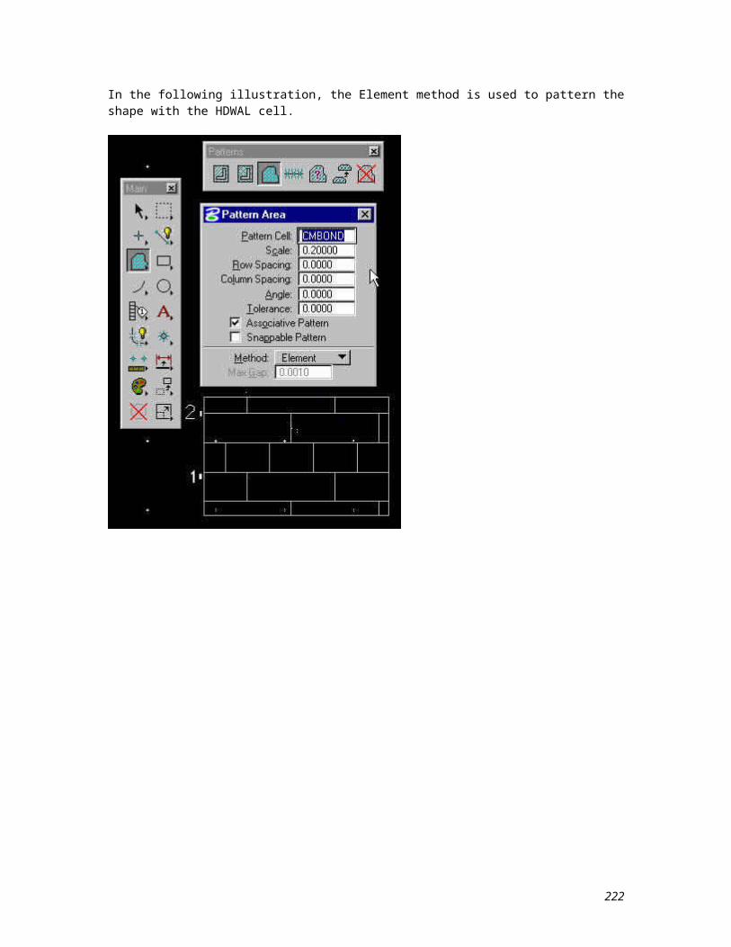
16.11 Reference File Level Symbology
The Level Symbology dialog box can also be used to control the level symbology for reference files. Even though it is the same dialog box, you will have to access it from a different menu.
To set the level symbology for a reference file:
1. From the Reference Files settings box, select the desired reference file from the list.2. From this settings box's Settings pull-down menu, select the Level Symbology item. This will display
the Level Symbology dialog box. The reference file number and name will appear in the bottom left corner.
3. Set the level symbology in the same manner you would for the active design file.
222
222

16.12 Fit Design and Reference Files
keyin: fit all
The Fit All view control allows you to make every visible element in the design display and all attached reference files in a selected view. If every element in a design has been drawn on one area of the design plane, this control works well. However, if elements have been drawn on many areas of the design plane, performing a fit may cause the elements to appear very small or as bright dots within the selected view.
223
223
16.13 Detach Reference File
keyin: ref det
Reference files stay attached to your active design file until you detach them. This tool is used to detach a reference file from the active design file.
To detach a reference file:
1. Select the Detach Reference File tool. 2. If necessary, identify the reference file. 3. The following alert box will appear:
Select the OK button to detach the reference file and dismiss the alert box, or select the Cancel button to dismiss the alert box and not detach the reference file.
224
224
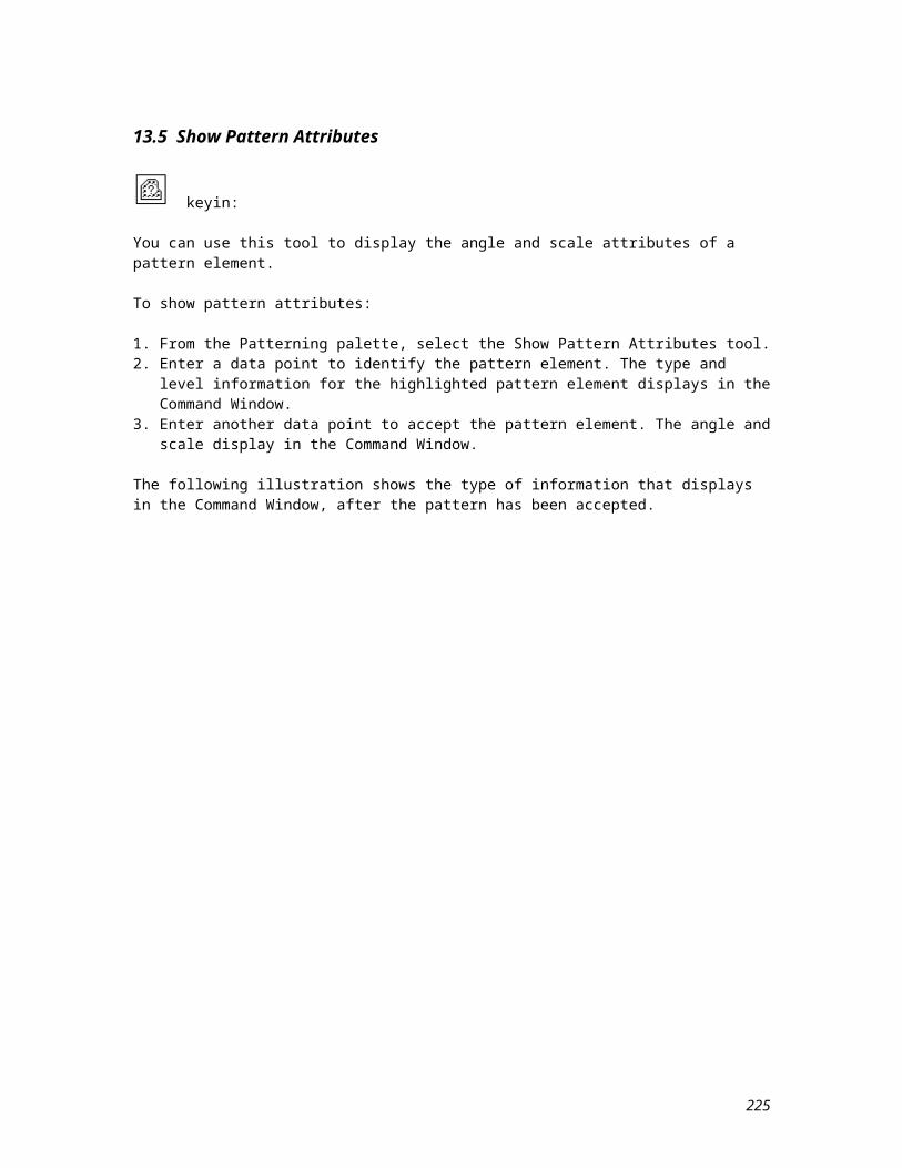
Lesson 17 - Dimensioning
225
225
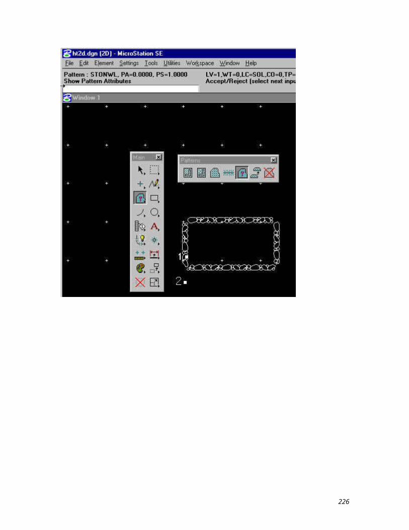
Lesson 17 - The 3 D Environment
The procedure for creating 3D files is essentially the same as it is for creating 2D files. The only difference is in what seed file is used. Seed files, like other design files, contain settings and view configurations. MicroStation has discipline-specific seed files, as well as the generic seed files, such as SEED2D.DGN and SEED3D.DGN. In some 3D seed files, a cube is drawn with construction elements to assist the beginning 3D user with standard orientations. The display of these construction elements can be turned off through the View Attributes settings box.
226
226
17.1 Design File Concepts
In 2D, remember that your design is on a plane that is parallel to the screen. The global origin is the center of the plane with the coordinates of (0,0). A 2D design plane has 4.29 billion positional units or units of resolution (UORs) in each direction.
In 3D, the design cube is a 3D implementation of the design plane. The design cube is an imaginary 3 dimensional volume. The design cube has three axes: X,Y, and Z. The X,Y, and Z axes correspond to length, width, and height when doing mechanical drawings. When doing construction drawings, the positive X,Y, and Z directions correspond to East, North, and Elevation. You can move around in the cube and see your design from any direction. By default, the global origin is the exact center of the design cube with the coordinates (0,0,0).
The design cube is 4.29 billion UORs on each side. As in 2D, you can specify the number of UORs per subunit and subunits per master unit in the working units dialog box. The smaller the number of UORs, the larger the dimensions of the design cube. The larger the number of UORs, the smaller the dimensions of the design cube; therefore you have greater accuracy.
227
227
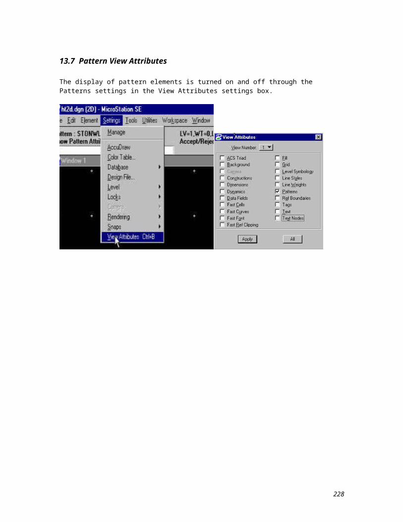
17.2 Views in 3D
To understand view orientations think of them as eight different people each holding a camera at eight different angles viewing the same object. One individual may be looking at the object from the front, one from the back, one from the right, one from the left, one from the top, and one from the bottom. These eight different perspectives correspond to eight views in a 3D file in Microstation.
The actual plane in each respective view will be parallel to the screen. If a pre-defined configuration of views is not setup in a seed file the default view orientation will be a Top view. This view equates to what you basically work with in a 2D file.
A 3D file there are eight standard view orientations:
Top Bottom Left Right Front Back Iso (showing Left, Top, and Front) Right Isometric (showing Right, Top, and Front)
228
228
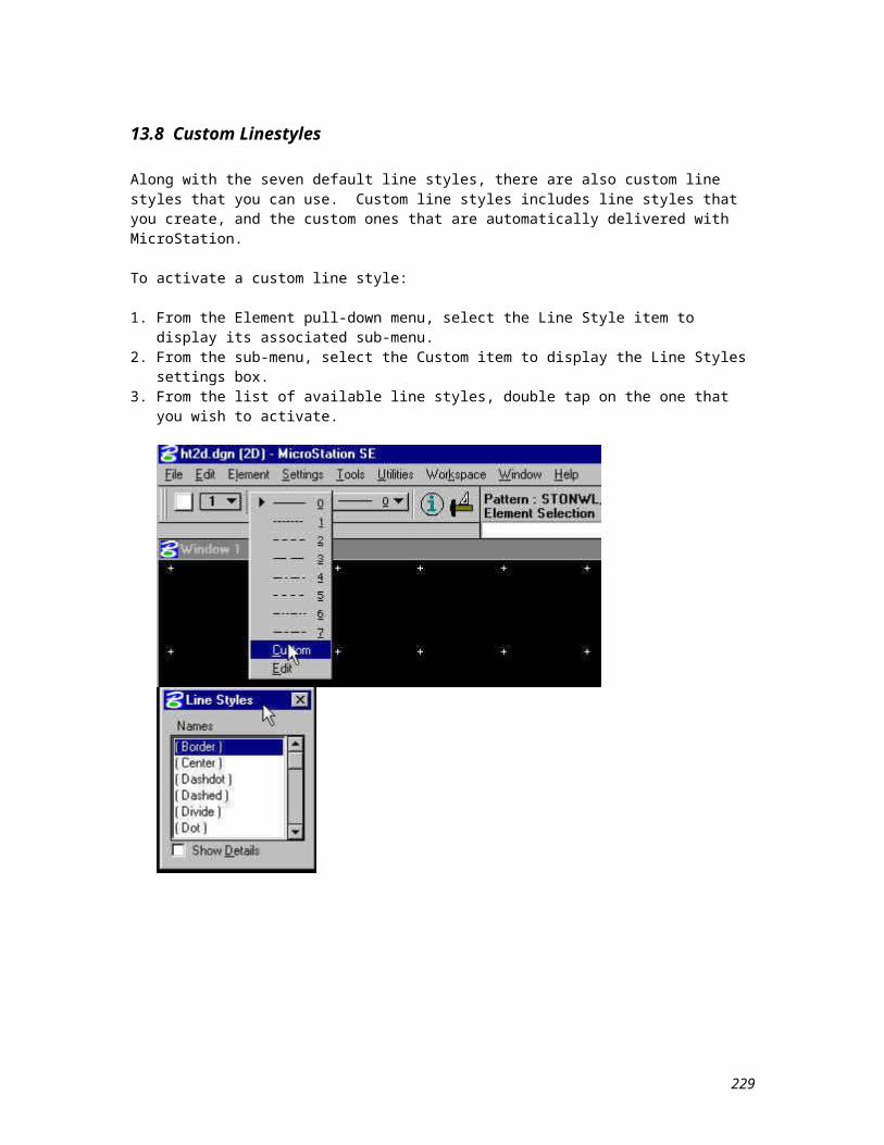
These views can be defined with the keyin vi= (the above mentioned view orientations), or with the View Rotation setting box.
229
229
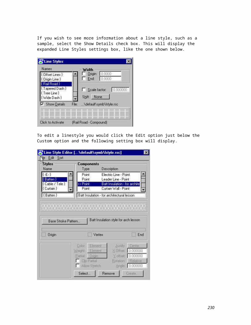
17.3 View Control
The following sections will detail the elements of view control in a 3D file. The concepts described will be the display depth, active depth and how to establish these parameters in each view that is opened in the 3D environment. Below is the 3D View Control palette.
230
230
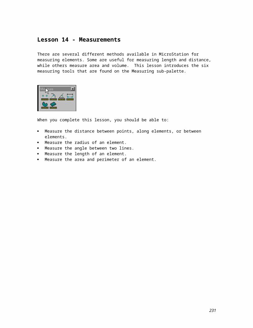
17.3.1 Display Depth
keyin: dp= (back plane, front plane)keyin: set ddep abs (front plane, back plane)
Each respective view that is setup in a 3D file will have its own view cube. You can determine how much volume a view cube encloses by defining a front clipping plane (the surface of the view cube which is closest to you along the Z-axis), and a back clipping plane (the surface farthest from you along the Z-axis). The distance along the Z-axis between the front and back clipping planes is called the display depth. Only elements that lie within the display depth can be seen in that view.
The default display depth is set in the seed file you create your map file with. If you specify the same plane for the front and back of the view cube, an error message is generated and the display depth can be seen in that view.
If you use the palette option to set the display depth in a view you must have at least two views open. Below is the process to set the display depth with the above mentioned command:
1. Select the Set Display Depth tool from the palette.2. Select the view for the display depth to be set by clicking in it (data point 1).3. Enter a data point to define the front clipping plane of the view cube (data point 2). You should enter
this point in a view other than where the depth is being set. If the point is entered in the view being set, the active depth is used.
4. Enter a data point to define the back clipping plane of the view cube (data point 3).
The keyin command sets the front and back clipping planes for a given view a specified distance from the global origin along the view’s Z-axis. The keyin command that you use will depend on whether the front or back plane is the first value specified.
231
231
17.3.2 Show Depth Display Control
keyin: sho depkeyin: dp=$
The Show Depth Display control shows the location of the front and back clipping planes of a view relative to the global origin. The values are displayed in the command window.
To show the Display Depth:
1. Select the Show Display Depth control.2. Select the view.
Below is an illustration of how the display depth is conveyed in the command window.
232
232
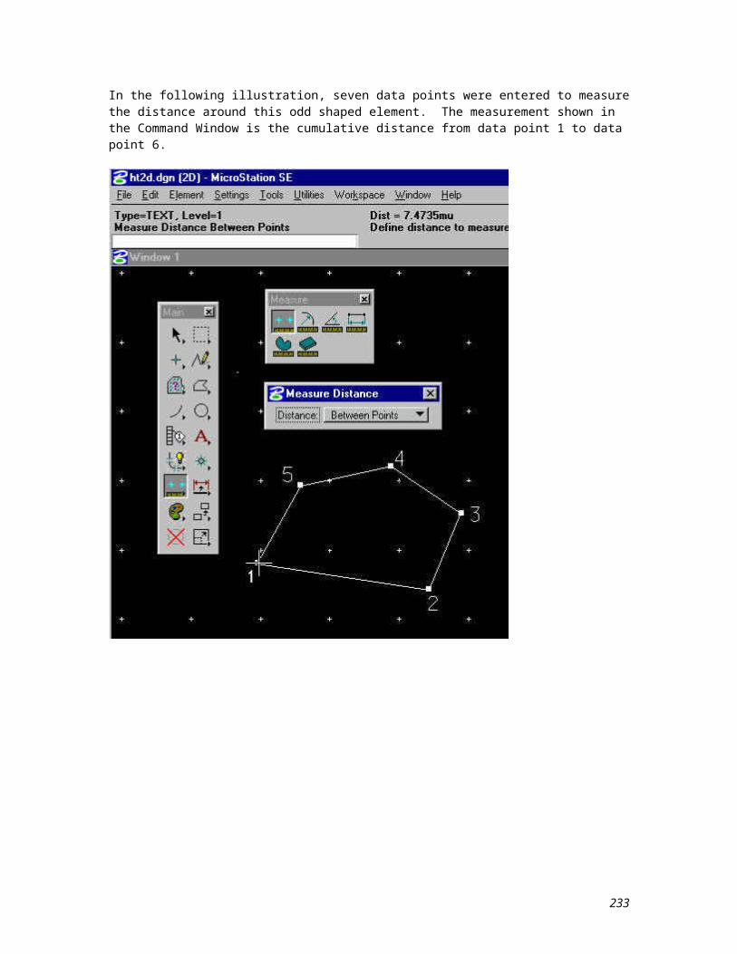
17.3.3 Active Depth
keyin: az= (digitizing depth)keyin: act zde (digitizing depth)
The active depth defines the actual plane/elevation that you will digitize on. The active depth is the plane/elevation that all data points fall, except when you snap, use precision inputs, Auxiliary Coordinate Systems, or 3D data or tentative points. The active depth/elevation is always parallel to the screen, and must always fall within the display depth.
Typically this setting is used when digitizing contour lines at various elevations to model the terrain of a given area. Digitizing of this type of data must occur in a Top View. To see the reflective contours at their elevations you will need to open a Front View. This permits you to face the mountain, hill or terrain that you are modeling.
To set the active depth:
1. Select the Set Active Depth tool.2. Select the view in which to change the active depth by clicking in it (data point 1).3. Enter a data point in a view (other than the view being set) that coincides with the desired depth of the
view being set (data point 2).
233
233
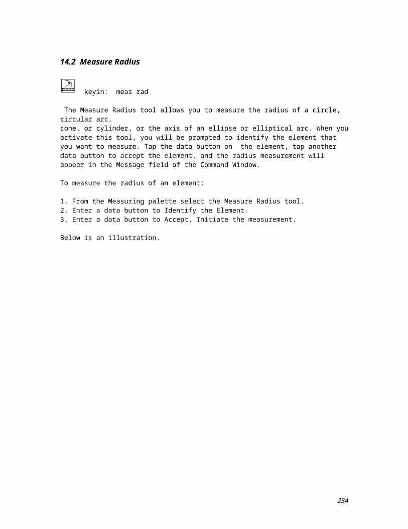
17.3.4 Show Active Depth Control
keyin: sho dep actkeyin: az=$
The show active depth control displays a view active depth. The value is displayed in the command window.
To show the active depth in a view:
1. Select the Show Active Depth tool.2. Select the view.
Below is an illustration:
234
234
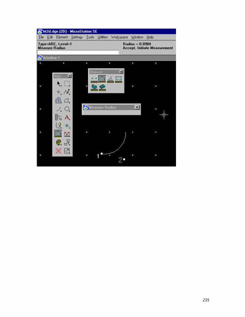
17.4 3D Elements
The following sections will describe 3D elements that are utilized in mapping, GIS and civil engineering applications. The elements are space linestrings and curvestrings. These element types will allow you to define vertices for one occurrence of an element between different elevations. You simply change the active depth between the placement of the vertices to define either the linestring or curvestring.
235
235

17.4.1 The Place Space Linestring Tool
keyin: pla lstr spa
The place space line string tool is used to place a 3D (non-planar) line string. A line string element can have a maximum of 101 vertices. If more than 101 vertices are defined, MicroStation automatically creates a complex chain consisting of one or more line string elements.
To place a space line string:
1. Select the Place Line String tool and select Non-planar.
2. Enter a data point to define the beginning of the line string.3. Continue to enter data points, or use precision input to define the vertices of the line string in 3D space.4. Reset to end the line string.
236
236
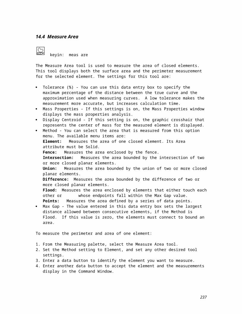
17.4.2 The Place Space Curve Tool
keyin: pla cur spa
The place space curve tool is used to place a 3D (non-planar) curve. A curve element can have from 3 to 97 vertices. If more than 97 vertices are defined, MicroStation automatically creates a complex chain consisting of one or more curve elements.
To place a space curve:
1. Select the Place Curve tool. Select the Points method and the Non-planar toggle button.
2. Enter a data point to define the beginning of the curve.3. Enter a second data point for the first curve segment.4. Enter a third data point to complete the first curve segment.5. Enter additional data points to add segments to the curve.6. Reset to end the curve.
237
237
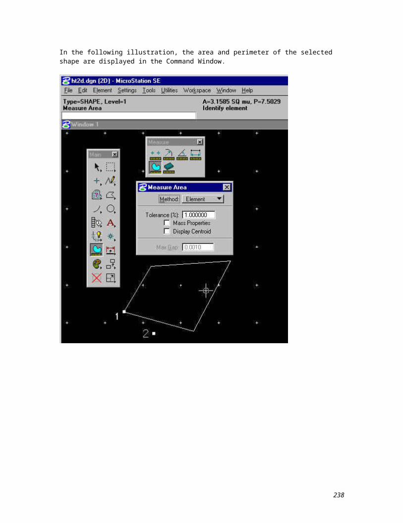
Lesson 18 - Plotting
MicroStation lets you get hard copy of your design file through the creation of a plotfile and the transmission of this plotfile to a plotting device. MicroStation supports a wide variety of plotting devices.
The easiest way to produce a plotfile in MicroStation is through the Plotting dialog box. This box, like the one shown below, is displayed by activating the Command Window File pull-down menu and selecting the Plot item. From this dialog box, you can preview a plot, set plotting settings, and create a plotfile. Plotfiles can then be submitted to a plotter to produce a hardcopy of your design.
The various objects found on this dialog box are explained in detail throughout the remaining pages of this lesson.
238
238
18.1 Deciding What to Plot
One of the first things that you will want to do is to decide on the area to be plotted. Two methods can be used to plot areas in your drawing. One method is to place a fence around the area that you want to plot. This method allows you to tightly control what will be plotted. The other method is to plot one of the eight design views/windows. While this method doesn't allow for as tight a control as the fence, it is possible to resize and/or refocus a view very tightly around the desired area. The following objects on the Plotting dialog box determine which method you will be using to generate your plotfile:
A plotfile can be created from a fenced area, if a fence exists in the design file. The Use Fence check button/box is automatically selected if a fence exists in your design, and it is dimmed if a fence does not exist. If it is selected, clicking on it will disable plotting by fence, and permit you to plot one of the eight views.
The plot view is chosen by selecting the desired view number from the View option menu. This option menu is dimmed if the Use Fence button is selected.
239
239

18.2 Choosing a Plotter
After you have decided what you want to plot, you must then decide what type of plotter you want to plot to. A plotfile is created using a specific configuration file for the selected plotter. This file is used to convert the graphic elements to an instruction set that the plotting device will use to draw the elements. The appropriate file must be selected first, since a plotfile created for a laser or electrostatic plotter probably would not plot on a pen plotter, or vice versa.
The plotter configuration filename always displays in the upper left corner of the Plotting dialog box. If this is not the configuration file that you desire, you can select the Plotters button to display the Plotter Configuration File dialog box, as shown below. This permits you to select the configuration file associated with the desired plotter. This file controls the available page sizes and most of the other settings. If a new file is selected after you have changed the page size, options, etc., those changes will be reset to the default values of the new plotter. These configuration files are located in the MicroStation plotcfg subdirectory. They will all have a .plt extension.
240
240
18.3 Setting the Page Size
In the Plotting dialog box, the black outer block represents the size of your plotter page. The blue inner block represents the printable area for the plot. This inner block will be proportional to the fence or view used to define the printable area. MicroStation will automatically calculate the largest plot that will fit on the selected page size. The Page Settings portion of the Plotting dialog box shows you the name and dimensions of the currently selected page.
When you select the Page Size button, the Set Page Size dialog box displays. This dialog box allows you to select the page name; paper sizes A, B, C, D, and E. The selections are dependent on the plotter configuration file currently selected. The Printable Area Dimensions and Offset from Paper Origin values are set based on the Page Name selection.
241
241
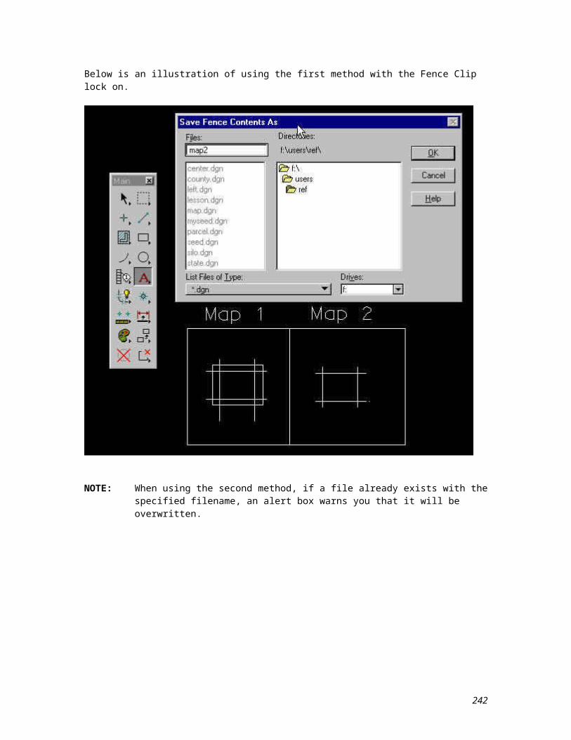
18.4 Plotting Options
There are several plotting options that will impact the plot file that will be sent to the plotter for hardcopy generation. These parameters consist of Microstation View Attribute settings. The Fence Boundary and Plot Border settings can be toggled on and off at within this Setting Box.
242
242
18.5 Plot Preview
The Plot Preview will display a preview to the screen of what will be plotted. This is based on the plotting parameter you have established. Below is an illustration of the Plot Preview function.
243
243
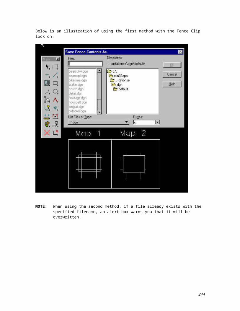
18.6 Plot Configuration Files
Plot configuration files can be constructed for the parameters that you setup for the plotting process. These files can be reused or modified at a later time. Below is an illustration of how to access the Plot Configuration utilities.
244
244
18.7 Plot Submission
Once you have your plotfile created, you can submit it to your plotter to produce a hardcopy. Below illustrates how a plot is submitted through Microstation.
245
245
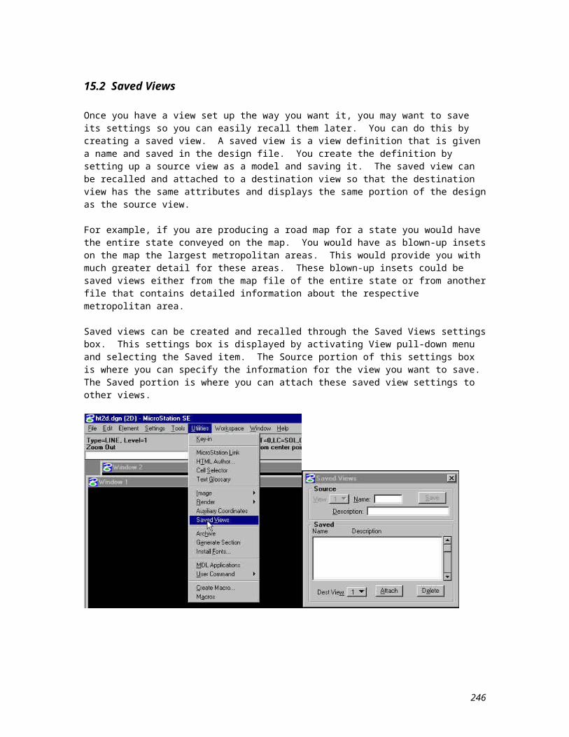
Lesson 19 - Introduction to Relational Database and Relational Interface System (RIS)
This lesson will consist of an overview of the structure of a relational database management system and the Relational Interface System (RIS). A description of how RIS interacts with the relational database will also be discussed. An introduction to some terminology that is frequently used when building a GIS with Intergraph products will also be presented.
246
246
19.1 Relational Database Overview
A relational database is a collection of related pieces of information. These pieces of information may be broken down into tables, field, and records for further organization within the database.
A field (column-descriptive attribute) is a specific characteristic in describing an item, such as the owner of a parcel of land. A record is a group of related fields (i.e.: owner, acreage, and assessed value for a parcel of land). A collection of records, all containing information about the same type of things such as a group of parcels, would be referred to as a table.
Below is a simple illustration of the table structure of the database:
Examples of database management systems that Microstation can communicate with are Informix, Oracle, INGRES, Sybase, RDB, DB2, OS4000, and MSSQL. Each of these respective databases has individual conventions and keywords that cannot be used for the creation of a tablename or a column.
247
247
19.2 The Relational Interface System (RIS)
RIS is a generic relational database interface. It isolates applications from the relational database, thus allowing the application to be compatible with several different database types. For instance, RIS will allow one set of source code for the MGE application to communicate with the different database management systems mentioned above. RIS utilizes the industry standard Structured Query Language to peruse and update the database.
RIS will create a schema to the respective database created by the database management system. The RIS schema is a pointer between RIS and the relational database that stores information such as the structure of the database (columns, data types, etc.), the tables and views within the database, the location of the database, database username, and any privileges associated with that user. If changes (table structure or updates) to the database are made at the underlying database level RIS, and thus MGE, will not see the changes until the table has been excluded from the schema and then included again.
248
248
19.3 Microstation Graphics - MGE correlation
In a basic cartographical drafting environment there is no interaction with a database, and thus there are no linkages that are written on the graphic elements that are placed to represent map features. Thus, the elements used to represent map features are considered non-intelligent or dumb graphics.
This is not the case when building a Geographic Information System with the MGE suite of products. A database structure is involved with this process that will assign intelligence to the map features that are digitized in their respective files. This means that a linestring in the framework of the project database can understand that it represents a road. This type of intelligent linkage is called a feature linkage. The feature linkage will point to a standard MGE product table describing the graphic characteristics of the feature (i.e.: line style, line weight, color, level, etc.). Beyond this, a higher level of intelligence can be assigned to the line, so that the linestring knows which road it is. This type of linkage is called an attribute linkage, and it points to a user-defined attribute table in the database.
Microstation is a component part of the GIS solution set. It is the primary graphics engine for the GIS applications. Below is an illustration of the modular approach to building a GIS solution set.
249
249
250
250