MAPPING CRIME FOR ANALYTIC PURPOSES: LOCATION QUOTIENTS ...€¦ · MAPPING CRIME FOR ANALYTIC...

MAPPING CRIME FOR ANALYTICPURPOSES:

LOCATION QUOTIENTS, COUNTS, ANDRATES

by

Patricia L. Brantingham

Simon Fraser University

and

Paul J. BrantinghamSimon Fraser University

Abstract: Crime can be analyzed and mapped in a number of differentways. This article compares maps of violent crime across the cities of Brit-ish Columbia utilizing three crime measures: counts, rates and crime loca-tion quotients (LQCs). The LQC, adapted from regional planning, providesviews of crime patterns not obtained with the two more traditional meas-ures of crime. When used in conjunction with crime counts and rates, theLQC offers a way of understanding how one area is different from anotherfor purposes of research and deployment of prevention and control re-sources.

Crime and its contextual backcloth exist at many spatial and tem-poral levels of resolution, from the international scene to the individ-ual crime site, from the trends of centuries to the patterns of seconds(Brantingham and Brantingham, 1993, 1984; Brantingham et al.,

Address correspondence to: Patricia L. Brantingham, School of Criminology,Simon Fraser University, Room WMC-1630, Burnaby, BC V5A 1S6, CAN (e-mail:pbrantin@sfu .ca).

264 — Patricia L. Brantingham and Paul J. Brantingham

1976). That is, crime can be studied, analyzed and dealt with atmany different levels of aggregation in time and space. Meaningfulcrime analysis can be done, for instance, at international levels, atnational levels, across smaller areas that range from regions to statesto counties to cities, and at detailed levels within a particular city —even down to the street block or individual address level. Temporalanalyses can sweep across centuries, can examine a set of years,months, days, hours, minutes or seconds. Over the past decade,mapping has become a key tool for crime analysts seeking to under-stand the patterns of crime (see, e.g., Block et al., 1995), enablingthem to see or visualize differences and similarities across time andspace.

Analyses of individual criminal events and of individual person,building or street victimization studies are currently of great interest(Clarke, 1980, 1992), but for practical purposes individual criminalevents must be aggregated in order to assess patterns and devisemethods for addressing them (e.g., Kohfeld and Sprague, 1990; Ken-nedy and Forde, 1990; Normandeau, 1987; Brantingham et al., 1991;Cusson, 1983, 1993). The variety of questions open to the crimeanalyst and the level in the cone of resolution used in analysis willalways vary with the type of problem being considered. In addition,the type of crime measure used in analysis will vary with the problemunder consideration.

This article explores how questions about crime, measures ofcrime and levels of resolution are linked conceptually, and how crimeanalysis can be improved by mapping different measures of crimeand comparing the results. The article illustrates this by mappingthree different crime measures — the crime count, the crime rate,and the crime location quotient (LQC) — at the interurban level ofresolution, utilizing 1994 crime data from the 68 separate municipalpolicing jurisdictions in British Columbia, CAN.1

A particular emphasis is placed on crime location quotients be-cause this is a relatively new technique for criminologists. The LQCwill be described in more detail later in this article, but it is basicallya method of measuring the relative mix of different types of crimes fora particular area compared to the mix in surrounding areas. For ex-ample, a city such as Tucson or Virginia Beach can have a relativelylow robbery rate but still have neighborhoods in which robberymakes up a relatively high proportion of all crimes compared to thecity as a whole. Robbery is a problem in such neighborhoods evenwhen it is not a problem citywide. Conversely, robbery can make up avery high proportion of offenses in a city such as San Francisco or

Mapping Crime for Analytic Purposes — 265

Newark, but within such "robbery* cities there will be subareas inwhich robbery represents a low proportion of crimes. Such propor-tional mixes are independent of total crimes in an area, and reallyrepresent a local crime "specialization."

As will be shown in this article, when used in conjunction withcrime counts and crime rates, LQCs offer a way of understandinghow one area is different from another for purposes of research anddeployment of prevention and control resources. This article focuseson city-level data, but the LQC can be used for comparison of statesor nations on the one hand or for comparison of regions, cities orneighborhoods on the other. The LQC can be used for comparison ofthe crime mix in different decades within centuries in historical re-search, or for comparison of the crime mix within the different hoursof the day in thinking about deployment of police during differentshifts. It is a tool that can be used at different levels of spatial andtemporal resolution.

STATISTICAL CRIME ANALYSIS

There is a need for constant improvement and innovation in meth-ods of analysis, no matter what questions are being asked or whatlevels of resolution are being studied. Methods are constantlychanging. The methods used by criminologists frequently originatefrom other disciplines such as sociology, psychology, geography, sta-tistics or mathematics. These are not static disciplines. Interestingly,many currently used techniques had their origins in studies of crimi-nal events. For instance, in statistics both Quetelet (1842) and Pois-son (1837) focused on the study of crime. Galton, Pearson and Yulewere all concerned, among other things, with developing statisticaltechniques that could be used to understand crime, as both heredi-tary and social problems (Stigler, 1986).

This article describes and maps the LQC, a new type of crimemeasure borrowed from the related disciplines of regional economicsand regional planning. The location quotient (LQ) is used in regionalplanning and regional economics to look at relative local economicactivity. LQs will be described in some detail after a brief review ofcrime counts and crime rates.

Crime analysis in the tradition of Guerry (1831) and Quetelet(1842), and as conducted by most criminologists, looks at crime asan aggregate measure for some summary unit. The most commonsummary measures are crime counts and crime rates based on po-

266 — Patricia L Brantingham and Paul J. Brantinqham

lice-recorded offenses, victimization rates based on survey estimates,and offender rates based on surveys and judicial convictions data.

Crime counts are used to assess the locations of "hot spots," as-sess police work loads and estimate future resource needs. Police,after all, must respond to discrete events, not estimates or ratios. InCanada, crime counts take the form of "actual crimes." These repre-sent events recorded as crimes following a preliminary investigationthat has established that a "reported crime" has in fact occurred.Crime rates, in contrast, are used to assess the risk of crimes occur-ring to particular types of people in particular locations or at par-ticular times, and to assess trends discounted for changing condi-tions (such as population growth). Crime rates are particularly usefulin planning prevention campaigns and in assessing the impact ofchanging social conditions of the risk of crime. Crime rates use somemeasure of crime occurrence as a numerator and units at risk as adenominator. The numbers in the numerator and denominator vary.Ideally the numerator is some measure of events or occurrences, andthe denominator is the most direct measure of units at risk. Whenthe numerator is a personal crime, the denominator frequently is thenumber of people residing in the aggregation area. When the nu-merator is residential breaking and entering, the denominator fre-quently is the number of dwelling units.

There are always problems with such crime measures. The countof events, based on official data, is usually an undercount both be-cause some crimes are not reported to police and because countingand recording rules typically record only the most serious offense inany complex criminal transaction. Such counts do, however, appearto be good measures of serious offenses and of offenses involving lostproperty covered by insurance (Litton and Pease, 1984; Brantinghamand Brantingham, 1984; Gove et al., 1985). There are difficulties ob-taining reasonable estimates for denominators when the potential"victims" move or are moveable. Boggs' (1960) work began the explo-ration of how patterns change as the denominator in the ratiochanges. For example, an auto theft rate based on a residentialpopulation ratio produces a very different picture of high- and low-crime areas in a city from that produced by a rate calculated usingthe number of automobiles present in the different areas. Boggs'(1960) work has been carried many steps further by Harries (1991);both show the interesting variability in what is "seen" as denomina-tors change.


LOCATION QUOTIENTS

Location Quotients (LQs) are a measure developed in regionalplanning and economics to try to address questions of the relativestructure and importance of local economies, while conceptuallyavoiding some of the stationarity problems of spatial analysis. Localareas are placed within a wider comparative context for analysis. Re-gional science has always looked for ways to compare activity at met-ropolitan or regional levels of aggregation.

LQs were developed to indicate activity in one area compared to itssurrounds. For example, within a metropolitan area the city centerwill contain most of the commercial activities. Rural farming areasalso have commercial centers: some small towns provide minimumessential goods and services; slightly larger towns provide a largerarray of goods and services for a wider area encompassing a numberof the smaller towns and their hinterlands; while finally a major citywill provide a much wider range of specialized goods and services to amuch larger region encompassing many hinterlands, small towns,and larger towns. Each town, however, is a commercial center, al-though the volumes of business in the smaller towns make it difficultto see them as commercial centers from the perspective of large cities.Still, the small town commercial centers may provide the same coremix of commercial activities (albeit with less choice of suppliers) pro-vided in the largest cities. When the smaller towns and large citiesprovide the same mix of goods and services, they may be functionallyequivalent even though their volumes of activities are very different.Rural towns attract business from the hinterland; large cities attractbusiness from the hinterland and from the rural towns.

Similar considerations can be seen at work across the neighbor-hoods and communities within large cities. Bedroom neighborhoodsoften have small local commercial and entertainment districts; largersubdivisions have local shopping malls, bar clusters, multi-screentheaters; and finally, the urban center has a dense business, enter-tainment and industrial concentration that attracts people from allparts of the metropolis. Commuting between areas is the modern ur-ban way of life.

Before this article describes the way LQs are calculated, it shouldstart to become clear that such relative measures have a use in crimeanalysis. Within a country such as the U.S. certain states and citiesdominate the total counts of crimes or have the highest crime rates.However, even in lower crime states or cities, there can be certaintypes of crimes that are disproportionally present compared to theirsurrounding areas and disproportional compared to the mix in

268 — Patricia L Brantingham and Paul J. Brantingham

The LQ assumes a "normal" distribution in a "standard" area, thatis, a "normal" number of jobs in a certain category in a "standard"area. Within regional sciences this normal number is used as ameasure of the amount needed to satisfy regional demand (self-sustainability). When the local amount falls below the normal

higher-crime-rate cities or states. For example, 40 or 50 robberies ina city in a low-robbery state such as Idaho or Wisconsin may makethat a relatively high-robbery city in context. In contrast, a city with40 or 50 robberies in a high-robbery state such as California wouldbe a relatively low-robbery city. This type of relative specialization canhave meaning in crime analysis, particularly when the analysis isrelated back to the relative mix of other socio-economic conditions.

From the planning perspective, the primary purpose of analysis isoften to make predictions about future activity, and to base thosepredictions on the way the area under study functions in relation toits surrounding area. What happens in one city is seen to depend notonly on what happens in other cities but also on what happens orwhat exists in surrounding resources. For example, what happens inVancouver or New York or Madrid depends on what happens in otherlarge cities, but also on what happens in the local areas surroundingthem. The interrelationship between and within urban areas, andbetween urban and rural areas, is complex. Relationships can be ex-plored within any particular urban area as well as between urbanareas. What happens in one neighborhood can be compared to whathappens in surrounding neighborhoods.

Equation 1 presents the basic formula for a Location Quotient inRegional Science (Klosterman et al., 1993). While many economic ac-tivity indicators might be used, LQs are frequently calculated on thebasis of employment. Employment can be defined in many ways, butis frequently divided into service, manufacturing, secondary and pri-mary extraction groups. Each of these may be subdivided repeatedly,working down to detailed types of employment.


amount, it is assumed that goods (or services) are exported. Equation(1) shows the ratio for importing or exporting. The numerator countsthe number of persons employed in a particular type of job in a spe-cific area divided by the total employed in that area. The denominatoris a similar ratio for a comparison surrounding area that may beused as the "normal" distribution for the "standard" area. The equa-tion can be formulated for different study areas and different catego-ries of employment, and can involve comparison with different stan-dard areas. While there are obvious problems with this measure inregional science, it does provide the potential for a relative crimemeasure in criminological studies.2

USE OP LOCATION QUOTIENTS IN CRIMINOLOGY

In criminology, of course, Location Quotients would use crimes asthe basic unit of count. Equation (2) restates the Location Quotientformula in criminological form:

Using an LQC, some towns and cities would be identified as cen-ters for violent crimes; others, as centers for property crimes. Someare centers for robbery; some for burglary; some for automobile theft.The center in one region might not appear to be a center when com-pared to centers in other regions. This is similar to a small town be-ing a center of commerce in a rural area but not in a large urbanarea. It is perhaps more important to note that, since this is a relativemeasure, a center cannot have high LQs for all crimes. It is a meas-ure that identifies relative area specialty in crimes.

The advantage of an LQC in crime analysis is that there is no needto obtain a count of the number of targets as is necessary in calcu-lating a crime rate. The LQC for robbery would be based on counts ofrobberies and all crimes,3 not population or number of target busi-nesses. The LQC for motor vehicle theft would be based on vehicle


thefts and total crimes, not the number of people or the number ofmotor vehicles. In this way, the LQC minimizes the problems high-lighted by Boggs (1960) and Harries (1991) in their discussions ofwhich types of denominator variables to use in constructing rates fordifferent types of crimes. Stationarity is still a problem, but can beaddressed by recalculations for different time periods.

Table 1 provides a hypothetical example of how LQCs work. In thisexample there are five states listed (States A to E) as well as a na-tional total for all index offenses and for robbery. As can be seen inthe table, robbery makes up 5% of index offenses nationally. State Ahas a low number of robberies but has the same robbery rate asState B, which has the highest number of robberies and the highestrobbery rate. State A has an LQC greater than State B. This meansthat while these two states have the same robbery rates, State A hasa higher proportion of robbery offenses compared to the national pro-portion than does State B. They are both high rate states, but State Ashows a "preference" for robbery compared to State B. Robbery is alarger part of the total crime problem in State A than in State B. StateC has the same high robbery rate as State A and State B, but it has amuch lower total crime rate than would be expected from the na-tional trend. Consequently, State C has a LQC 7 times what would beexpected from the national trend. State D and E both exhibit low rob-bery rates but have LQCs similar to State A. Although robbery ratesare low, they make up a relatively large share of the crime problem inboth States D and E. The point is that LQCs do not necessarily "copy*crime rates or crime counts. They are really a dimensionless measureof preference or choice of crime type in the smaller unit compared toa larger trend.

Table 1: Location Quotient Example: HypotheticalStates


The LQC provides an additional, alternative view of crime. It is nota rate and is not a percentage. The LQC is without dimension; it is arelative measure. When a study area (be it a state, a city or a neigh-borhood) has an LQC equal to 1.00 for a specific crime, that meansthat it has a proportional mix of that crime similar to the larger com-parison area (country, state or city). When the value of the LQC fallsbelow 1.00, the relative proportion of that crime in the smaller studyarea is below the normal trend in the larger comparison area. Whenthe LQC is above 1.00, the specific crime is above the normal trend.In fact, the amount above 1.00 indicates the percentage above thenormal trend. In Table 1, State A has an LQC value of 1.4, meaningthat it is 40% higher than the national trend for robbery. State B hasan LQC value of 0.7, or is 30% below the national trend. State C hasan LQC of 7.1, or is 610 % above the national trend! Robbery is themajor crime problem in State C. States D and E both have low rob-bery rates, but robbery is a relatively greater problem in the latterthan in the former.

Statistical models using LQCs are different from the models mostcommonly constructed by criminologists. LQCs are relative measuresand are potentially helpful when analyzing fear or concern aboutcrime. A widespread fear of murder by a stranger can be triggered ina small community by one local crime, while a similar level of fearmight require clear evidence that a serial killer is active before beingtriggered in a large urban center. Similarly, one or two bank robber-ies might seem like very little in New York City, but a large number insmaller towns like Flemington or Montauk. LQCs may also provegood predictors of local media response to specific reported crimes oreven to variations in sentences in different places at different times.

LQCs are also indicators of what attracts people, both locally andfrom a distance, to a particular location. Some crime sites are crimegenerators; others are crime attractors. Crime generators are placesthat attract large volumes of people, generating criminal opportuni-ties in the process. Some of the people attracted to a generator loca-tion will notice those opportunities and act on them even though theyhad not been intending to commit any crime in the first place. Crimeattractors are places notorious for providing opportunities for crime.Offenders travel to crime attractors with the preestablished intentionof committing some specific crime there (see Brantingham andBrantingham, 1995).

LQCs also have a statistical model-building strength. In manymodels using crime rates, the independent and dependent variablesare both rates based on population. In such instances, the overall


strength of the model may be the result of the same numbers beingused as the denominators on both sides of the equation. With LQCs,the independent variable would not have the same base. Independentvariables may even reflect routine activities in the LQ form. For ex-ample, a measure of the number of bars to total number of busi-nesses in a town can be compared to the ratio for the region underanalysis. It seems reasonable that as the local ratio begins to exceedthe regional ratio, the LQC for violent crime would also increase. Thiswould not necessarily be found in an analysis of violent crime rateswhen population is used as the denominator. It might not even befound if the number of bars were used as the denominator in con-structing crime rates.

It should be noted that LQCs are ratio variables, and, like all ratiovariables, can be influenced by substantial changes when the ratiosare calculated from very small numbers. LQCs have a numerator anda denominator. The numerator is the only part of the equation thatcan have small numbers. For example, when the analysis is of areaswith low levels of crime, a change from 20 to 25 recorded crimes of aspecific type could have an impact on the calculated value of the LQCwhen the total local-area crime count is also low. Such a substantialimpact might be reflected in local-area fear levels in particular. Sucha possibility warrants exploration of past reported crimes in smallcrime-volume areas. It could be that in small areas with low crimetotals, such as city blocks or Census tracts, a three-year average ofcrime counts should replace an annual total to smooth out fluctua-tions and ensure stability in the LQC. In fact, LQC analysis usingmoving averages or autoregressive functions may become useful intime-series analyses that examine the evolution of concentrations ofspecific types of crime in specific areas. This is worth future research.For example, as an area grows or declines the crime rate might notchange, but the crime mix might change quite substantially. Thiswould make the crime problem faced by residents and police alikequite different, even though the volume of crime remained the same.LQCs offer a potential for exploring area crime specialization overtime.

While LQCs have many strengths, it is worth noting that thismeasure, like all other measures of crime, is dependent on a classifi-cation schema. That is, limits are introduced when crimes are dividedinto property/violent clusters, or specific criminal code violations orindex crime categories. This is another conceptual level of resolution.While not addressed in this article, LQCs could be used in numerouscategories initially or could be staged. They could first be calculated


for violent and property crimes in two categories. After that, violent orproperty crimes could be divided into subcategories and LQCs recal-culated. Each approach would inform the researcher about some-thing slightly different. For example, which specific crimes are differ-ent from the general trends, or, within a category such a violentcrimes, which types of violent crimes are different from a restrictedcomparison to violent crime trends. While it will not be discussed inmore detail in this article, the hierarchical nature of classification ofcrimes may reveal fine but important differences between areas.

It is also important to note that there is value in looking atchanges in LQC from one time period to another. A change in a spe-cific crime LQC can signal a dramatic change. If the LQC increases itmeans that there has been a shift in the local dominance of thatcrime. If the LQC for that crime decreases it means that there hasbeen a decrease in the local dominance of that crime. Unlike crimerates or crime counts, LQCs operate within fixed numeric limits. Theset of areas forming the full area under consideration will togetheraccount for the full area crime totals. There will be areas with LQCsgreater than 1.00, less than 1.00 and equal to 1.00. LQCs may go upwhen total or specific crimes decrease, and may go down when spe-cific crimes go up. The LQC is a relative measure without a dimen-sion. LQCs are like changes in the proportion of persons who die froma specific disease. All people die. When the proportion goes down forone cause it increases for another cause. These proportional changes,such as an increase in a particular cause of death, may occurwhether the death rate increases, decreases or remains stable.

Over all, the LQC offers an additional view on crime and poten-tially has value in understanding crime patterns. Counts and ratesare not sufficient; volume dominates both. LQCs are relative meas-ures of crimes that show how a specific area varies from generaltrends. Context is imbedded within LQCs.

Mapping Crime Patterns: An Illustration

To illustrate the different things that can be learned from analyz-ing the patterns of crime counts, crime rates and LQCs, we use 1994data on crimes known to the police in 65 municipal forces in BritishColumbia. The basic data are population counts, total criminal codeoffense counts and total violent crime4 counts for each city. Datawere geocoded to Universal Transverse Mercator (UTM) NAD 27, Zone10 centroids for each municipality using Maplnfo for Windows. Mapspresented in this discussion were generated using Stanford Graphicsand Maplnfo.


The substantially different pictures of crime obtained by looking atcounts, rates and LQCs are illustrated in Table 2, which presents thetop 15 ranked British Columbia cities in terms of violent crimecounts, violent crime rates, and LQCs for violent crime.

Violence counts are, unsurprisingly, tied to city size. Vancouver,the largest city and largest policing jurisdiction in the province,ranked first in violent crime counts. Surrey, the second largest juris-diction, and Burnaby, the third largest, ranked second and third inviolent crime counts respectively. Outside the Greater Vancouverarea, the other large population centers — including the provincialcapital, Victoria, and three large interior population centers — alsoranked highly in terms of violent crime counts. These are the hotspots where police and the rest of the justice system will have to dealwith a large number of violent crimes and criminals, and where themedical system and insurance schemes will have to deal with largenumbers of victims.

This pattern is mapped in abstract two-dimensional form in Fig-ure 1. The axes plot UTM Northing and Easting coordinates. Citiesare positioned in their relative locations in geographic space. Theview is from the south, looking due north.. There is a major hot spotin the southern part of the province, anchored by Vancouver, Surreyand Burnaby. The black-and-white depiction does not do justice towarm spots in the Okanagan Valley, where Kelowna is located, andon the southern end of Vancouver Island, where Victoria is located.5

These are the areas that require resources keyed to volumes of vio-lent victimization.

Crime rates, of course, tell a very different story. In this case, ratesare calculated by dividing the violent crime counts for each city by itsestimated 1994 population. Rates are expressed as violent crimes per1,000 population. The British Columbia cities with the highest ratesof violent crime are smaller cities in the northern and northwesternparts of the province. These areas are depicted as hot spots in Figure2. Most of these cities are service and recreation centers for largehinterlands: fishers, forest workers, miners and ranchers come tothese cities looking for entertainment.6 Liquor consumption is highand assaults in particular occur with substantial relative frequency.

These cities characteristically have relatively low volumes of crime,but should concentrate crime prevention planning efforts on violence.People in these cities run a much higher risk of violent attack thanresidents in the larger cities of the southern parts of the province.The crime-count hot spot centered on Vancouver becomes a crime-


rate cold spot once crime per unit volume of population is considered.This pattern is also mapped in Figure 2.

Table 2: Top Ranked Cities for Three Crime Measures

278 — Patricia L. Brantingham and Paul J. Brantingham

LQCs for violent crime across British Columbia cities tell yet an-other story. Cities with high LQCs for violent crime are those in whichviolent crime makes up a much higher proportion of the total crimeproblem than is characteristic of the provincial pattern generally.Although some high-rate cities will also have high LQCs, many willnot. Some cities with relatively low total crime counts and relativelylow violent crime rates will have high LQCs because violent crimemakes up a disproportionate share of all the crimes that occur inthat municipality when compared to the provincial pattern in general.Kitimat, for instance, ranks second in LQC, but only 24th out of the65 cities in terms of violent crime rates. Kimberly ranks 12th interms of LQC, but only 46th out of the 65 cities in terms of violentcrime rate. This means that although the overall risk of crime is rela-tively low in these cities, those crimes that do occur are much morelikely to be violent ones than in most other cities in the province.

The converse can also be true: some cities will have relatively highviolent crime rates, but those rates will be embedded in such highoverall crime rates that any particular crime is not much more likelyto be a violent crime than it would be in other, far less crime-pronecities. Williams Lake is an example of such a place: it ranks firstoverall in terms of violent crime rate, but 18th in terms of LQC. Wil-liams Lake's LQC of 1.33 for violent crime indicates that its violentcrime mix is above the normal pattern for the province as a whole,but not extremely so. Some cities will have high violent crime counts,low violent crime rates and very low LQCs for violent crimes.Burnaby, for instance, ranked third in terms of violent crime counts,35th in terms of violent crime rates but 54th out of the 65 cities interms of LQC. This indicates that a substantially smaller proportionof Burnaby's crime mix involves violent crimes than is typical of thecrime mix in the province generally. This means that any particularcrime occurring in Burnaby would be less likely to be a violent crimethan any particular crime occurring in the province at large. ThatLQCs and rates tell different stories is apparent from regressing rateson LQCs. Violent crime rates explain only about half the variation inthe LQCs.

Figure 3 maps the LQCs for violent crimes for British Columbiacities. The North Cowichan area of Vancouver Island stands out ashaving a much higher proportion of all its crime take the form of vio-lence than is normal for the province as a whole: it is depicted as anLQC hot spot. A northwestern warm spot is also visible. Violent crimemakes up a smaller-than-expected proportion of the crime mix in the


large population centers in Greater Vancouver and the southern partof Vancouver Island, which generally appear as cold spots.

Violent crime counts, violent crime rates and LQCs for violentcrime are mapped across the police jurisdictions of the Vancouverand Victoria metropolitan areas in Figures 4, 5 and 6. Violent crimecounts show hot spots in Vancouver and Surrey, the two largest mu-nicipalities in British Columbia. These counts are population driven.Violent crime rates show a very different picture, with hot spots inthe city of Victoria and in North Cowichan on Vancouver Island, andin Langley City, a small suburban bright-lights district in the metro-politan Vancouver district. LQCs show yet a different pattern to vio-lent crime. The entire Vancouver region has relatively low LQCs, indi-cating that violent crime makes up less of the crime mix in this re-gion than it does in the province as a whole. North of Vancouver, tworesort destinations — Sechelt, a coastal community, and theSquamish-Whistler ski-resort area — show violent LQCs that aresubstantially above provincial levels. On Vancouver Island, the NorthCowichan area and the municipality of Esquimalt, adjacent to Victo-ria, have very high LQCs. These communities experience substan-tially more violence per unit of crime than the province as a whole.

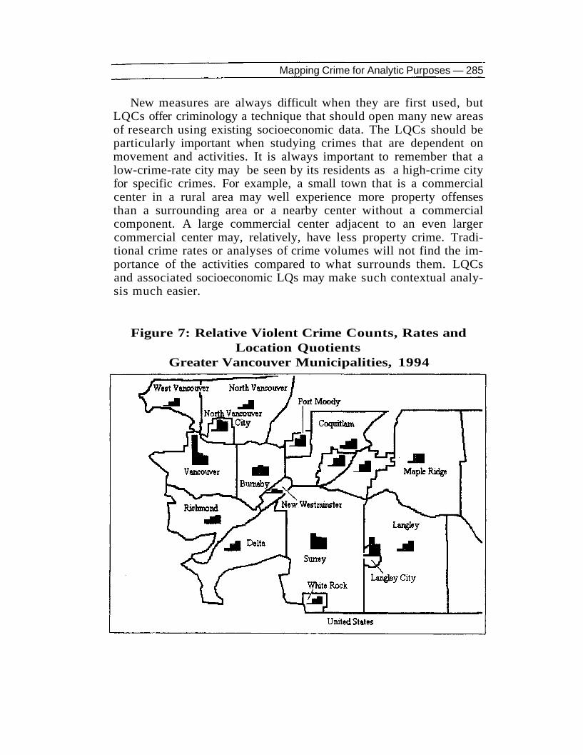
A more immediate mapping of the differences in the three crimemeasures is seen in Figure 7, which focuses on the municipalities ofGreater Vancouver. Bar charts present first the violent crime count,then the violent crime rate, then the LQC for violent crime in eachmunicipality.7 Vancouver, the largest city in the metropolitan area,stands out in the left center of the map. Vancouver displays a veryhigh violent crime count, a substantially lower violent crime rate, anda much lower LQC for violence. Although a large number of violentcrimes occur in Vancouver, a much smaller proportion of its totalcrime mix comprises violence than is typical of the province as awhole. This suggests that Vancouver's crime mix is relatively benign(if such a term can ever be applied to a crime problem), and that thecity has a more intense problem with property and other types ofcrime rather than with violence.

Although a more detailed situational analysis would be necessary,it appears that high priority in crime prevention planning ought to beplaced on reduction of property offenses and other nonviolent of-fenses. In contrast, many of the municipalities adjacent to Vancouverproper have relatively low violent crime counts. But of the few crimesthat occur in these municipalities, many more are violent than wouldbe typical of the province as a whole. In these municipalities, crimeprevention efforts should focus on the violent crime attractors and


generators in an effort to reduce the volumes of situations that sup-port violent crime. Here much can be gained through attention to theproblems of violence. This understanding of the need to develop crimeprevention programs aimed at reduction of violent crime would bemissed if the main focus of crime prevention planning were either thecrime counts or the crime rates for these communities. Some of thecommunities with very low violent crime counts and crime rateswould benefit more from attention to violent crime than would othersimilar-sized communities that have reputations for violence prob-lems but that in fact have relatively low LQCs.

Mapping crime counts and rates and LQCs together can providevery useful visual information that helps identify some importantcharacteristics of local crime problems. It also provides insight intoresource needs, crime risks for citizens at large, and the preventionstrategies and priorities that could most profitably be pursued.

CONCLUSION

Crimes occur on a backcloth (Brantingham and Brantingham,1993): at whatever level of analysis is pursued (macro, meso, micro),it is important to see how specific crime type occurrences relate tocrime in general. LQCs provide a measure that helps identify whethera specific crime pattern is disproportionately high or low in a par-ticular place or location. While LQCs should not be used withoutconsidering counts and rates, they do provide a relative or contextualview of crime and should prove helpful in understanding crime pat-terns and in developing priorities and approaches in crime preven-tion.

While not the focus of this article, LQCs should have great valuein research into the prediction of crime patterns. Relative socioeco-nomic and relative activity measures may turn out to be good pre-dictors of crime patterns in ways that more traditional measures havenot. The use of LQ measures should make it possible to develop pre-dictor variables that reflect activity, movement and the actual varietyin use where different activities occur. Data sources for aggregateanalysis can begin to include economic measures, as well as Censusand survey information. Mapping relative use measures may prove aparticularly useful tool for criminologists and crime prevention pro-fessionals alike.


New measures are always difficult when they are first used, butLQCs offer criminology a technique that should open many new areasof research using existing socioeconomic data. The LQCs should beparticularly important when studying crimes that are dependent onmovement and activities. It is always important to remember that alow-crime-rate city may be seen by its residents as a high-crime cityfor specific crimes. For example, a small town that is a commercialcenter in a rural area may well experience more property offensesthan a surrounding area or a nearby center without a commercialcomponent. A large commercial center adjacent to an even largercommercial center may, relatively, have less property crime. Tradi-tional crime rates or analyses of crime volumes will not find the im-portance of the activities compared to what surrounds them. LQCsand associated socioeconomic LQs may make such contextual analy-sis much easier.

Figure 7: Relative Violent Crime Counts, Rates andLocation Quotients

Greater Vancouver Municipalities, 1994


NOTES

1. Twelve jurisdictions maintain independent municipal police forces.The remainder contract with the Royal Canadian Mounted Police, whoprovide municipal policing services through autonomous municipal de-tachments. A similar arrangement is found in many American jurisdic-tions. The Los Angeles County Sheriffs' Department provides contractedmunicipal policing services to a substantial proportion of the independ-ent cities in the county. Other cities in the county — Los Angeles or LongBeach, for instance — maintain their own independent forces.2. Clearly, the Location Quotient approach has limitations in regionalscience. With major cities being linked economically, it is not possible toactually identify what activity in a "standard" area would be. This issimilar to identifying what a "standard" crime pattern would be. In actualpractice, LQs mean more for their relativity and defined context, which istaken as the "standard" for logical purposes.

3. LQC is a relative measure, so the denominator can be flexible. Forinstance, with robbery in the numerator, the LQC might be calculatedusing the count of all violent crimes, the count of all criminal code of-fenses, or the count of all offenses known as the denominator, dependingon the context in which the analyst wished to comprehend robbery cen-ters.

4. Violent crime in Canada includes murder, manslaughter, infanticide,attempted murder, sexual assault, assault, abduction and robbery.5. Most contemporary mapping packages work in color. This is a prob-lem for presentation in print media.6. This represents one of the denominator problems with crime rates.The actual usage of a city may greatly exceed the resident population.7. Note that these three sets of bars represent somewhat differentscales, as indicated in Table 1.

REFERENCESBoggs, S. L. (1960). "Urban Crime Patterns." American Sociological Re-

view 30:899-908.

Block, C.R., M. Dabdoub and S. Fregly (1995). Crime Analysis ThroughComputer Mapping. Washington, DC: Police Executive Research Fo-rum.


Brantingham, P.L. and P.J. Brantingham (1984). Patterns in Crime. NewYork, NY: Macmillan.(1993). "Environment, Routine and Situation: Toward a Pattern

Theory of Crime." Advances in Criminological Theory 5:259-294.(1995). "Criminality of Place: Crime Generators and Crime Attrac-tors." European Journal on Criminal Policy and Research 3:5-26.and P.S. Wong (1991). "How Public Transit Feeds Private Crime:Notes on the Vancouver 'Skytrain' Experience." Security Journal 2:91-95.

Brantingham, P. J., D. A. Dyreson and P. L. Brantingham (1976). "CrimeSeen Through a Cone of Resolution." American Behavioral Scientist20:261-273.

Clarke, R.V.G. (1980). "Situational Crime Prevention: Theory and Prac-tice." British Journal of Criminology 20:136-147.

Clarke, R.V. (ed.) (1992). Situational Crime Prevention: Successful CaseStudies. New York, NY: Harrow and Heston.

Cusson, M. (1983). Why Delinquency? Toronto, CAN: University of To-ronto Press.(1993). "A Strategic Analysis of Crime: Criminal Tactics and Re-sponses to Precriminal Situations." Advances in Criminological The-ory 5:295-304.

Gove, W. R., M. Hughes and M. Geerken (1985). "Are Uniform Crime Re-ports a Valid Indicator of the Index Crimes?" Criminology 23:451-501.

Guerry, A. M. (1831) Essai Sur la Statistique Morale de la France. Paris,FR: Chez Crochard.

Harries, K. D. (1991). "Alternative Denominators in Conventional CrimeRates." In: P.J. Brantingham and P.L. Brantingham (eds.), Environ-mental Criminology. Prospect Heights, IL: Waveland Press.

Kennedy, L.W. and D.R. Forde (1990). "Routine Activities and Crime: AnAnalysis of Victimization in Canada." Criminology 28:137-152.

Klosterman, R.E., R.K. Brail and E.G Bossard (1993). Spreadsheet Mod-els for Urban and Regional Analysis. New Brunswick, NJ: Transac-tion Publishers.

Kohfeld, C.W. and J. Sprague (1990). "Demography, Police Behavior, andDeterrence." Criminology 28:111-136.

Litton, R. A. and K. Pease (1984). "Crimes and Claims: The Case of Bur-glary Insurance." In: R. Clarke and T. Hope (eds.), Coping with Bur-glary. Boston, MA: Kluwer-Nijhoff Publishing.


Normandeau, A. (1987). "Crime on the Montreal Metro." Sociology andSocial Research 71:289-292.

Poisson, S.D. (1837). Recherch.es Sur la Probability des Jugements enMatiere Criminelle et en Matiere Civile, Precedes des Regies Genera-les du Calcul des Probabilites. Paris, FR: Bachelier.

Quetelet, A.J. (1842). Treatise on Man and the Development of His Facul-ties. Edinburgh, SCOT: W. and R. Chambers.

Stigler, S. M. (1986). The History of Statistics: The Measurement of Uncer-tainty before 1900. Cambridge, MA: Belknap Press of Harvard Uni-versity Press.

MAPPING CRIME FOR ANALYTIC PURPOSES: LOCATION QUOTIENTS ...€¦ · MAPPING CRIME FOR ANALYTIC...

Documents

Transcript of MAPPING CRIME FOR ANALYTIC PURPOSES: LOCATION QUOTIENTS ...€¦ · MAPPING CRIME FOR ANALYTIC...