A decade of participatory mapping – the road to Mapping for Change

The views expressed in this presentation are the authors’ and not necessarily those of the Federal
Reserve Bank of New York or the Federal Reserve System.
Mapping Change in Complex Financial
Markets
Inaugural Conference of the “Journal of Network Theory in Finance” , September 23,
2014. Cambridge Centre for Risk Studies, Cambridge University, UK

2
Martin Rosvall
Department of Physics
Umea University
Carl Bergstrom
Department of Biology, University of
Washington and Santa Fe Instititue
Morten Bech
BIS
Rod Garratt, FRBNY
Contributing Authors

3
U.S. Overnight Money Market

4
Interbank Claims (BIS Locational Data)

5
We need a way to see the important details of the network structure.

How do we make maps?

good maps simplify

Not helpful!

good maps simplify
and highlight

good maps simplify
and highlight
good maps simplify
and highlight
relevant structures


13
What is important in our context?
not trying to get from St John’s Wood to King’s Cross
We want to find the structures within the financial network that are important with respect to the flow of funds

14
Consider the overnight money market in the U.S.
The flow of funds is a large weighted, directed
network.
Individual banks are the nodes.
The value of loans from node α to node β determines
the weight on the directed link from α to β.
Normalized weights become transition probabilities
In order to understand lending relationships we
can use an information-theoretic network
clustering technique developed by Rosvall and
Bergstrom (2008)
Information-theoretic clustering
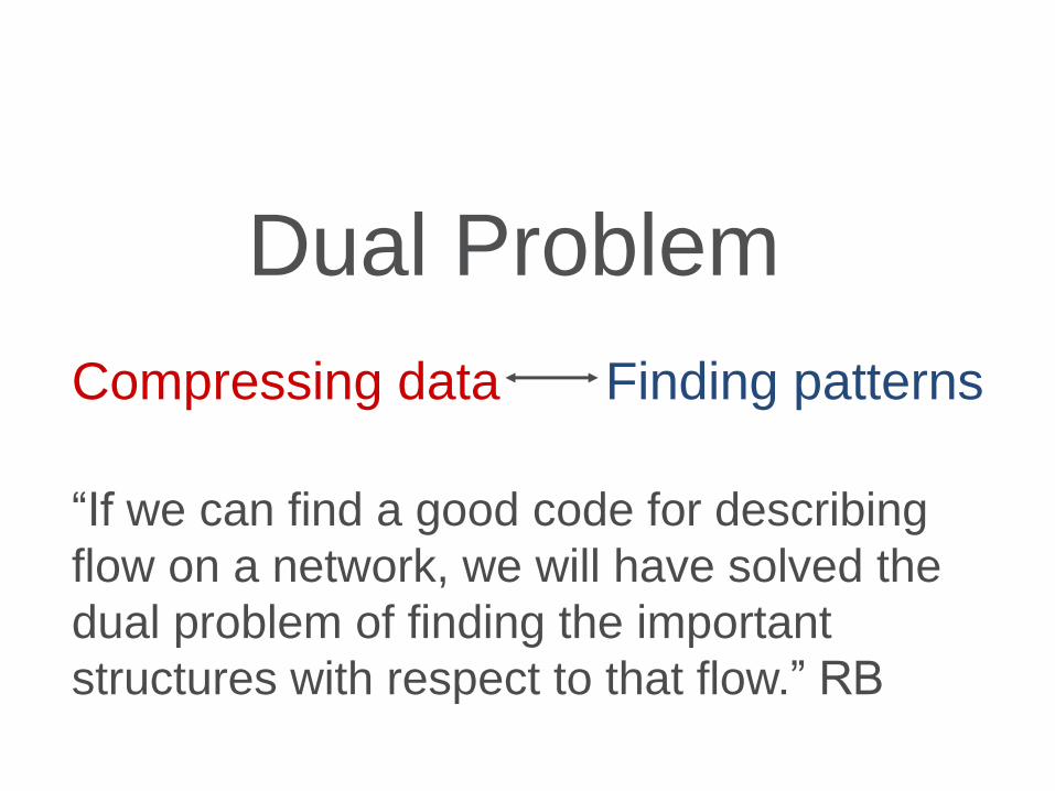
Dual Problem
Compressing data Finding patterns
“If we can find a good code for describing
flow on a network, we will have solved the
dual problem of finding the important
structures with respect to that flow.” RB
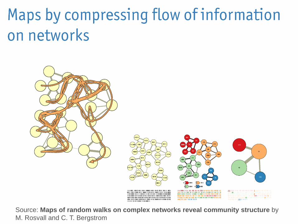
16 Source: Maps of random walks on complex networks reveal community structure by
M. Rosvall and C. T. Bergstrom

17

18
Huffman Code
1. At each step the characters you have seen do not yet
correspond to any item, or they correspond to exactly one
2. Encoded message is shortest satisfying 1.
1001110110010111 = cataract
Prefex free code: a receiver can identify each word without
requiring a special marker between words.
Symbol Code
a 0
c 10
r 110
t 111

19
Modular Structure
RB apply Huffman coding in a “tiered” way, saving code by using two types of code books
module codebooks & index codebook
Can reuse code words in different modules
Transforms the problem of minimizing the description length of places traced by a path into the problem of how we should best partition the network with respect to this flow
Trade-off costs and benefits measured in terms of bits

20

21

naming
places
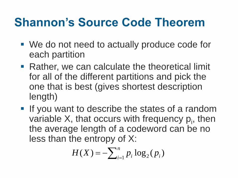
Shannon’s Source Code Theorem
We do not need to actually produce code for each partition
Rather, we can calculate the theoretical limit for all of the different partitions and pick the one that is best (gives shortest description length)
If you want to describe the states of a random variable X, that occurs with frequency pi, then the average length of a codeword can be no less than the entropy of X:
n
i ii ppXH1 2 )(log)(

24
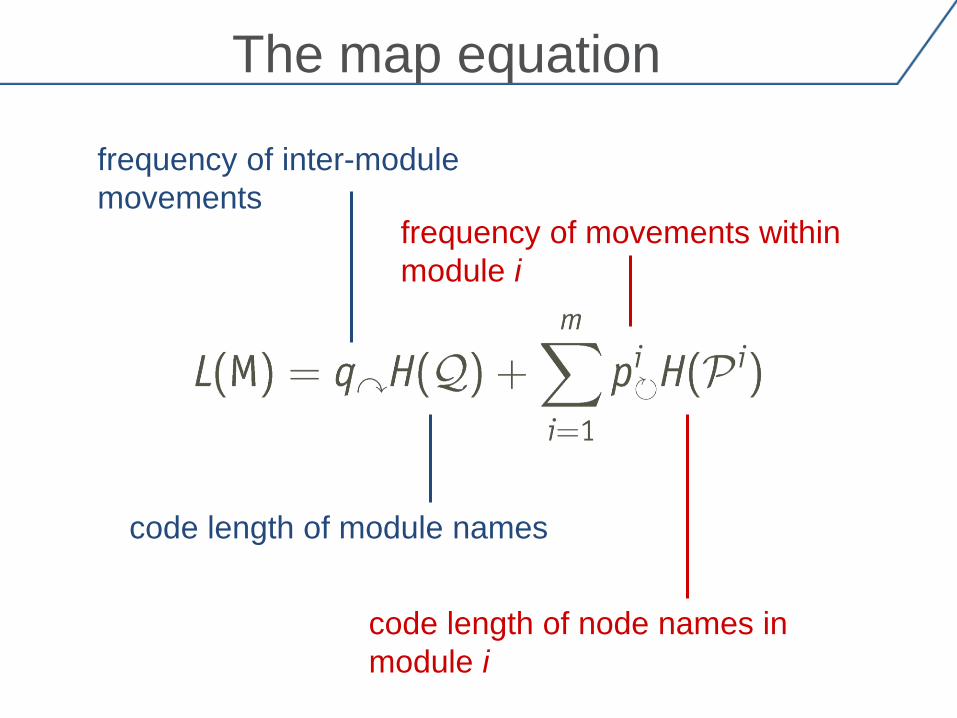
The map equation tells us the minimum
description length for a particular modular
structure
The map equation
25
frequency of inter-module
movements
code length of module names
frequency of movements within
module i
code length of node names in
module i
The map equation

Any numerical search algorithm developed to find a
network partition that optimizes an objective function can
be modified to minimize the map equation.
M. Bech, C. Bergstrom, R. Garratt and M. Rosvall, “Mapping Change in the
Overnight Money Market,” 2014, mimeo

Interbank Claims
2008 Q3
1989 Q3
R. Garratt, L. Mahadeva and K. Svirydzenka, “The Contagious Capacity of
the International Banking Network: 1985-2009, JBF, 2014.

28
Mapping Change
Alluvial Fan

Mapping change of payment flows driven by interbank lending market activity from July 2008 to December
2008.

The orange cluster is dominated by a set of Federal
Home Loan Banks and a number of small and medium
sized banks.
“...a combination of financial consolidation, credit losses,
and changes to risk management practices has led at
least some GSEs to limit their number of counterparties
in the money market and to tighten credit lines.” (Bech
and Klee, JME, 2011)

The fairly stable green cluster which is subsumed into the
large cluster after the implementation of interest on reserves,
is dominated by a prominent government-sponsored
enterprize and one large money center bank.
The break down of the cluster may reflect the reduction (or
even elimination) of the lending relationship to the particular
bank by the GSE.

The blue cluster is comprised of a Federal Home Loan Bank
and a number of banks that tend to be located the same
geographic region as the Home Loan Bank.
We speculate that this cluster reflects the fact that the Home
Loan bank may have started to intermediate funds between
its members by borrowing funds from some and making
overnight advances (i.e., collateralized loans) to others during
this period.
33
What are the key differences?
What is real change and what is mere
noise?
Need to know which structures are
statistically significant and which are not.

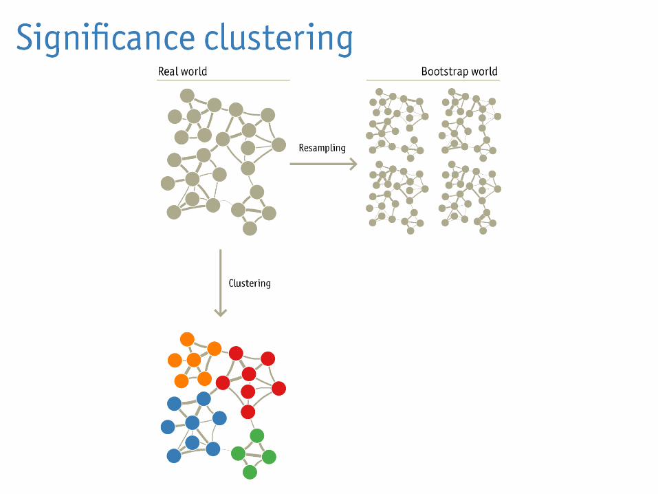
Source: Mapping change in large networks by M. Rosvall and C. T. Bergstrom


40
Analysis of Micro-Scale Rates of Change
While the alluvial diagrams are very nice for showing the
general patterns of how lending takes place in each period,
they do not necessarily reveal the onset of change in the
system.
Changes in clustering patterns reflect tipping points at which
the cumulative effect of multiple small changes in flows
constitute a significant change.

Transformative
Event: Lehman?

Transformative
Event: IOER?

43
Tipping Points
Suppose that lending configurations a, b, c, d, e, f, g, h all
generate a system with module structure of type 1, and
configurations i, j, k, l, m, n, o, p all generate a system with
module structure of type 2.
Most rapid change from period 2 to 3, not 4 to 5.
T= config cluster
0 a 1
1 a 1
2 b 1
3 g 1
4 h 1
5 i 2
6 j 2
7 j 2

44
Micro-Scale Rates of Change
We would like to be able to differentiate between the two
hypotheses that (1) Lehman's failure is associated with a
shakeup in lending patterns and (2) paying interest on reserves
is associated with the shakeup.
An n x n lending matrix is specified by a unique vector of
length n^2.
each time period corresponds to a vector in n^2 space.
To measure the amount of change in the system, we look at
how much the angle between the vector at each time t changes
going to time t+1.
This is a standard approach in network theory, known as cosine
distance.

Orange trace compares the distance between each time period and a fixed
time period (Sep 10).
Black trace shows us the velocity of change from one period to the next
over time.
Largest change occurs in the Oct 8 maintenance period, which covers the
time period from September 25 to October 8, after collapse of Lehman and
before IEOR.

46
Transformative Event
While changes in borrowing and lending patterns do not fully
reveal themselves in our maps until after the implementation of
Interest on Reserves, examination of the micro-scale rates of
change strongly suggests that the collapse of Lehman Brothers
was the driving force.

47
Concluding Remarks
Advanced network techniques can help stakeholders in the
financial system to understand its structural features and to
analyze the impact of transformative events.
As illustrated here, the map equation appears to be a very
useful tool for understanding funding flows.
More appropriate than “competing” techniques that impose
community structure or ignore flows
The lending flows in the interbank lending market changed in a
fundamental way between September 10 and October 22,
2008, and the alluvial diagrams reveal this clearly.
However, there is evidence that the underlying shifts in network
flows that led to these structural changes may have been
initiated well before the tipping point was reached.

48
Concluding Remarks
Considerable caution is required when deriving causal
inferences from alluvial diagrams.
We advocate the use of two tools for analyzing the structure
of financial networks.
Each complements the other and neither is sufficient in
isolation.
The map equation reveals community structure and changes
can be visualized via alluvial diagrams.
However, these maps do not reveal details of micro-scale
rates of change that precipitated change.
The cosine distance analysis is useful in this regard, but itself is
not informative: it reveals change, but not the content of that
change.

Thank You