Map-Reduce for Machine Learning on Multi-Core
73
Map-Reduce for Machine Learning on Multi-Core Gary Bradski, work with Stanford: Prof. Andrew Ng Cheng-Tao, Chu, Yi-An Lin, Yuan Yuan Yu. Sang Kyun Kim with Prof. Kunle Olukotun. Ben Sapp, Intern
Transcript of Map-Reduce for Machine Learning on Multi-Core

Map-Reduce for Machine Learning on Multi-Core
Gary Bradski, work with Stanford:Prof. Andrew NgCheng-Tao, Chu, Yi-An Lin, Yuan Yuan Yu.Sang Kyun Kim with Prof. Kunle Olukotun.Ben Sapp, Intern

2
AcknowledgmentsThe Map-Reduce work was supported by:
Intel Corp*. and byDARPA ACIP programWith much help from Stanford CS Dept.
I left Intel a month ago to join Rexee Inc.www.rexee.com
I maintain my joint appointment as a consulting Professor at Stanford University CS Dept.
*Some slides taken from Intel presentation on Google’s Map-Reduce andPaint slide from www.cs.virginia.edu/~evans/bio/slides/paintable.ppt

3
And Ad-Sense AdvertsOpen, Free for Commercial Use:
Open Source Computer Vision Libraryhttp://sourceforge.net/projects/opencvlibrary/
Machine Learning Libraryhttp://sourceforge.net/projects/opencvlibrary/
Optimized Support for Nominal $, Royalty free:Performance
http://www.intel.com/cd/software/products/asmo-na/eng/302910.htm

4
OpenCV: Open Source Computer Vision Lib.http://www.intel.com/research/mrl/research/opencv
Takes advantage of Intel® Integrated Performance Primitives (optimized routines)

5
Bayesian NetworksLibrary:
PNL
Statistical LearningLibrary:
MLL
• K-means
• Decision trees
• Agglomerative clustering• Spectral clustering
• K-NN
• Dependency Nets
• Boosted decision trees
Machine Learning Libraries (MLL)Subdirectory under OpenCV http://www.intel.com/research/mrl/research/opencv
Modeless Model based
Uns
uper
vise
dS
uper
vise
d• Multi-Layer Perceptron
• SVM• BayesNets: Classification
• Tree distributions
Key:• Optimized• Implemented• Not implemented
• BayesNets: Parameter fitting• Inference
• Kernel density est.
• PCA
• Physical Models
• Influence diagrams
• Bayesnet structure learning
• Logistic Regression
• Kalman Filter
• HMM
• Adaptive Filters
• Radial Basis • Naïve Bayes• ARTMAP
• Gaussian Fitting
• Assoc. Net.
• ART• Kohonen Map
• Random Forests.
• MART
• CART
• Diagnostic Bayesnet
• Histogram density est.

Talk

7
OverviewWhat is Map-Reduce?Can Map-Reduce be used on Multi-Core?
We developed a form for distributed algorithms:These forms can be expressed in a Map-Reduce framework as a parallel APIDynamic load balancing, Vision and MANY Core
Current projects and speculationsModel enabled vision.
8
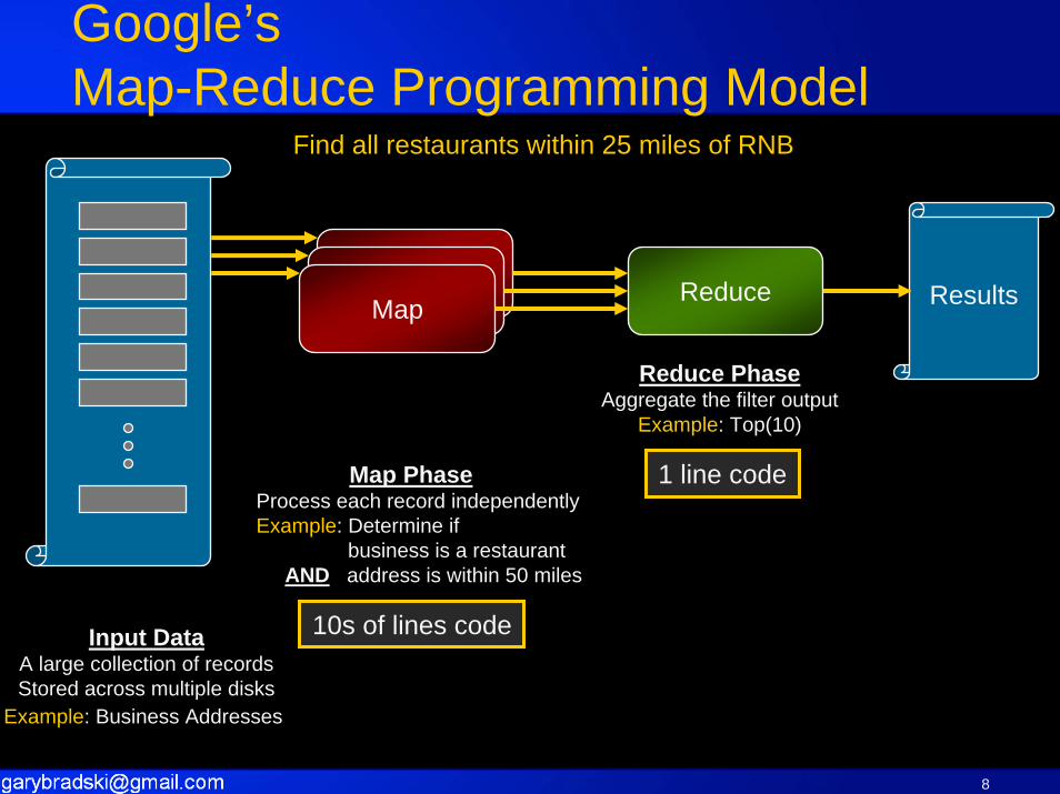
Google’sMap-Reduce Programming Model
Input DataA large collection of recordsStored across multiple disks
Example: Business Addresses
Map PhaseProcess each record independentlyExample: Determine if
business is a restaurant AND address is within 50 miles
Reduce PhaseAggregate the filter output
Example: Top(10)
FilterFilterMap
Reduce Results
10s of lines code
1 line code
Find all restaurants within 25 miles of RNB

9
More Detail:Google Search Index Generation
Web Page 3
Web Page 4
Web Page 5
Web Page 6
Web Page 1
Web Page 2
Web Page N
LexiconTable
FilterFilterFilterA
AggregatorA
In Reality, Uses 5-10 Map-Reduce StagesEfficiency impacts how often this is run. Impacts quality of the search.
WebGraph
FilterFilterFilterB
AggregatorB
PageRankTable
FilterFilterFilterC
AggregatorC

10
More Detail: In Use:Google Search Index Lookup
Google Web Server
Index ServerIndex ServerIndex ServerIndex ServerIndex ServerIndex ServerIndex ServerIndex ServerIndex ServerDocument Server
Spell Check Server
Ad ServerMap
Reduce
MapReduce
Processing a Google Search Query

11
MotivationApplication: Sifting through large amounts of dataUsed for:
Generating the Google search indexClustering problems for Google News and Froogle productsExtraction of data used to produce reports of popular queriesLarge scale graph computationLarge scale machine learningGenerate reverse web link graph
Platform: cluster of inexpensive machinesScale to large clusters: Thousands of machinesData distributed and replicated across machines of the clusterRecover from disk and machine failures

12
Google Hardware InfrastructureCommodity PC-based Cluster
15,000 Machines in 2003Scalable and Cost Efficient
Reliability in SoftwareUse inexpensive disks (not RAID)Use commodity Server
Data Replication: Data survives crashesFault Tolerance: Detect and recover─ Hardware Error─ Bugs in Software─ Misconfiguration of the Machine

13
Two Map-Reduce Programming ModelsSawzall
Simpler interpreted languageNot expressive enough for everything (use of intermediate results).
MR-C++Library that allows full control over Map-ReduceCan sometimes run much faster, butMuch slower to code/debug

14
Two Map-Reduce Programming Models1. MR-C++
C++ with Map-Reduce libProgrammer writes Map and Reduce functions
Relatively clean modelAllows workarounds─ Side-effects, Combiner
functions, Counters
Simplifies programmingAn order of magnitude less code than before
Efficient (C++)
2. SawzallDomain specific language
Programmer provides MapUse built-in set of Reduce
Clean modelEnforces the clean model─ If it doesn’t fit the model,
use the Map-Reduce
Even simpler programmingOften an order of magnitude less than Map-Reduce
Inefficient + “Good enough”Interpreter (50x slower)Pure value semantics

15
Map-Reduce Infrastructure Overview
Protocol BuffersData description language like XML
Google File SystemCustomized Files system optimized for access pattern and disk failure
Work QueueManages processes creation on a cluster for different jobs
Map-Reduce (MR-C++)Transparent distribution on a cluster: data distribution and scheduling
Provides fault tolerance: handles machine failure
Building Blocks
Programming Model and
ImplementationC/C++ Library
SawzallDomain Specific Language
Language

16
Map-Reduce on a Cluster
Find all restaurants within 25 miles of SAP
1. Use ClusterA. Locate DataB. Exploit Parallelism
2. Map Phase: Check each business3. Collect the list4. Reduce Phase: Sort by Distance5. Report the results6. At any stage: Recover from faults
These programs are complicated but similar.Map-Reduce hides parallelism and distribution from programmer (steps 1, 3, 5, & 6).
“Map” ServerRack
“Reduce” ServerRack
Heavily Loaded
Map
Reduce
Request

17
SearchIndex
NewsIndex
ProductIndex
Examples of Google Applications
Google SearchSearch Index Generation Search Index Lookup
Google News
Offline: Minutes to WeeksModerately Parallel
Online: Seconds per Query“Embarrassingly” Parallel
News Index Generation News Index Lookup
Froogle SearchFroogle Index Generation Froogle Index Lookup
100s of small programs (Scripts)Monitor, Analyze, Prototype, etc. IO-Bound

18
Google on Many-Core ArchitectureGoogle Workload Characteristics
Extremely Parallel, Shared Working-SetThroughput-orientedLow Available ILP
Confirmed by Google’s IndexBench BenchmarkExtension to Mulit- and Many-Core?
Hyperthreading → Multi-Core → Many-CoreDelivers more “Queries per Second per Watt”─ Simpler cores (efficiently use transistors)─ Reduce communication across machines─ Benefit from sharing caches and Memory

Map-Reduce on Multi-Core
Use machine learning to study.

20
OverviewWe developed a form for distributed algorithms:
Summation form─ Done for Machine Learning and Computer vision
These forms can be expressed in a Map-Reduce framework as a parallel API
Map-Reduce Lends itself to dynamic load balancing
Papers in accepted in NIPS 2006, HPCA 2007:

21
Summation form for Machine LearningBasically, any algorithm fits that learns by:
Computes sufficient statisticsUpdates by local gradientsForms ~independent “voting” nodes
22
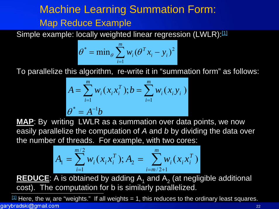
Machine Learning Summation Form:Map Reduce Example
∑=
−=m
iii
Ti yxw
1
2* )(min θθ θ
bA
yxwbxxwAm
iiii
m
i
Tiii
1*11
)(;)(
−
==
=
== ∑∑θ
∑∑+==
==m
mi
Tiii
m
i
Tiii xxwAxxwA
12/2
2/
11 )(;)(
Simple example: locally weighted linear regression (LWLR):[1]
To parallelize this algorithm, re-write it in “summation form” as follows:
MAP: By writing LWLR as a summation over data points, we now easily parallelize the computation of A and b by dividing the data over the number of threads. For example, with two cores:
REDUCE: A is obtained by adding A1 and A2 (at negligible additional cost). The computation for b is similarly parallelized.
[1] Here, the wi are “weights.” If all weights = 1, this reduces to the ordinary least squares.

23
Each implies an NxN communication
To be more clear: We have a set of M data points each of length N
)( Tii xx
ML fit with Many-Core
NMMMM
N
N
xxxx
xxxx
xxxx
,...,,...
,...,,
,...,,
21
222
122
121
111
=
=
=
N
N
Decomposition for Many-Core:
ThreadsT1
N
T2
. . .
TP
M
Each “T” incurres a NxN communication cost
bA
yxwbxxwAm
iiii
m
i
Tiii
1*11
)(;)(
−
==
=
== ∑∑θ
N<<M or we haven't formulated a ML problem
This is a good fit for Map-Reduce

24
Map ReduceWe take as our starting point the functional programming construct “Map-
Reduce”* and it’s use in Google allowing common massively parallel programming.
Map-Reduce is a divide and conquer approach:Map step: Processes subsets of the data in parallel with no communication
between subsets.─ Processing must result in “sparse” results such as sufficient statistics, small histograms,
votes etc.Reduce step: Aggregate (sum, tally, sort) the results of the map steps back to a central master.There may be many map-reduce steps in a single algorithm
We extend this concept to machine learning for multi-coreAnd will also extend to Computer vision next.
(*) Jeffrey Dean and Sanjay Ghemawat. “Mapreduce: Simplified data processing on large clusters”, Operating Systems Design and Implementation, pages 137–149, 2004.

25
Map-Reduce Machine Learning Framework
Programming Environment Block Diagram0 Engine subdivides the data1 Algorithm is run, appropriate engine invoked
1.1 Master is invoked by engine1.1.1 Data is mapped out to cores for processing1.1.2 Sparse processed data from cores is returned1.1.3 And aggregated by reducer1.1.4 Results are returned─ Other needed global info can be retrieved by query (1.1.1.1, 1.1.3.1)

26
List of Implemented and Analyzed AlgorithmsAlgorithm Have summation form?
1. Linear regression Yes
2. Locally weighted linear regression Yes
3. Logistic regression Yes
4. Gaussian discriminant analysis Yes
5. Naïve Bayes Yes
6. SVM (without kernel) Yes
7. K-means clustering Yes
8. EM for mixture distributions Yes
9. Neural networks Yes
10. PCA (Principal components analysis) Yes
11. ICA (Independent components analysis) Yes
12. Policy search (PEGASUS) Yes
13. Boosting Unknown*
14. SVM (with kernel) Unknown
15. Gaussian process regression Unknown
17. Multiple Discriminant Analysis Yes
18. Histogram Intersection Yes
16. Fisher Linear Discriminant Yes
Analyzed:

27
Complexity Analysis: m: number of data points; n: number of features; P: number of mappers (processors/cores); c: iterations or nodes. Assume matrix inverse is O(n^3/P’) where P’ are iterations that may be parallelized. For Locally Weighted Linear Regression (LWLR) training: (‘ => transpose below):==============================================================X’WX: mn2
Reducer: log(P)n2
X’WY: mnReducer: log(P)n(X’WX)-1: n3/P’(X’WX)-1X”WY: n2
Serial: O(mn2 + n3/P’)Parallel: O(mn2/P + n3/P’ + log(P)n2
map invert reduce
Basically: Linear speedup with increasing numbers of cores.

28
Some Results, 2 Cores
On 2 processor machine:
Dataset characteristics:
Basically: Linear speed up with the number of cores

29
Results on 1-16 Way SystemIn general, near linear speedup.Must have enough data to justify.Load time is often the bottleneck.
30
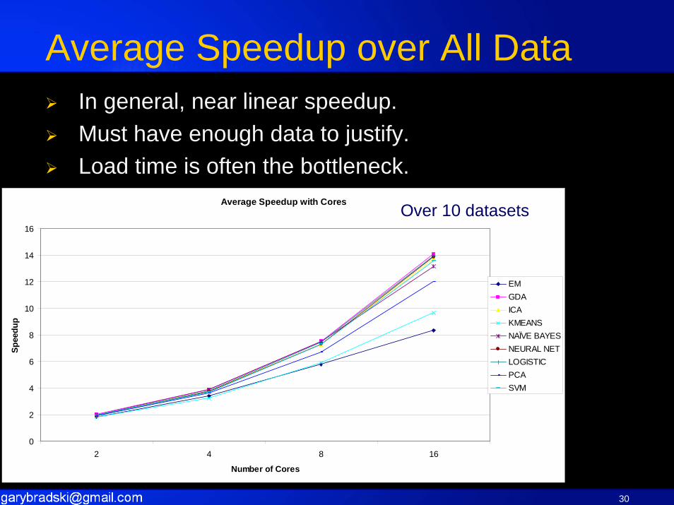
Average Speedup over All Data
Average Speedup with Cores
0
2
4
6
8
10
12
14
16
2 4 8 16
Number of Cores
Spee
dup
EMGDAICAKMEANSNAÏVE BAYESNEURAL NETLOGISTICPCASVM
Over 10 datasets
In general, near linear speedup.Must have enough data to justify.Load time is often the bottleneck.
31
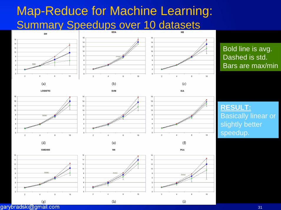
Map-Reduce for Machine Learning:Summary Speedups over 10 datasets
Bold line is avg.Dashed is std.Bars are max/min
RESULT:Basically linear orslightly betterspeedup.

32
SpeedupThe speedup for the total time becomes dominated by load time.The speedup for the workloads was near linear.The speedups for some of the workloads were limited by the serial region.─ Ex. PCA, EM, ICA, NR_LOGICSTICThe speedups for one of the workloads was limited by the reducer.─ Ex. K-mean
Workload vs. Data Set SizeThe workload time was roughly linear to the data set size, when the size was reasonably large enough.
Serial TimeMost of the serial regions had only a fixed amount of computation.The only exception is the PCA algorithm.We can see that the impact of the serial regions lessons while we increase the data set size.
Reducer Execution TimeThe reducer time for most of the algorithms do not scale with the size of data.─ Exception is the K-means algorithm, which increases linearly.The reducer time, however, scales with the number of processors.For most of the algorithms, the reducer execution time was insignificant.
Overall Results

33
Dynamic Run Time Optimization Opportunity
In the Summation form framework─ The granularity of the threads is flexible─ May be changed globally over time
Dynamic Optimization/Load Ballance Algorithm:─ Keep subdividing threads─ Until performance registers indicate performance fall-off.─ Step back towards larger granularity─ Periodically iterate

Discussion

35
Really want a Macro/micro Map-ReduceFor independent processing
Seemless over clusters of Multi-CoreFor 2-tier, learning across independent records
Map over clustersCall Map-Reduce machine learning routines
Should work well for algorithms like Kleinberg’s Stochastic DiscriminationBreiman’s Random Forests

36
Extension to Other Areas of AIWe’ve seen machine learningMap Reduce on Multi-Core seems to extend
To computer visionNavigationInference (loopy belief propagation)
37
Multi-Core here => Shared Memory, but…Map-Reduce spans bridge to non-shared memory
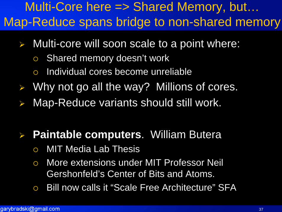
Multi-core will soon scale to a point where:Shared memory doesn’t workIndividual cores become unreliable
Why not go all the way? Millions of cores.Map-Reduce variants should still work.
Paintable computers. William ButeraMIT Media Lab ThesisMore extensions under MIT Professor Neil Gershonfeld’s Center of Bits and Atoms.Bill now calls it “Scale Free Architecture” SFA

38
Paintable Computing

39
ConclusionsMap-Reduce is an effective paradigm for Google.It can be usefully extended to support AI algorithms on Multi-coreBy dropping explicit masters, it can span Scale Free Architectures with Millions of distributed nodes.

References and Related Work

41
ReferencesMap Reduce on Multi-core:
Map-Reduce for Machine Learning on MulticoreCheng-Tao Chu, Sang Kyun Kim, Yi-An Lin, YuanYuan Yu, Gary Bradski, Andrew Ng, Kunle OlukotunNeural Information Processing Systems 2006.
Evaluating MapReduce for Multi-core and Multiprocessor SystemsArun Penmetsa, Colby Ranger, Ramanan, Christos Kozyrakis and Gary Bradski.High-Performance Computer Architecture-13, 2007.
Map Reduce at Google:
Interpreting the Data: Parallel Analysis with SawzallRob Pike, Sean Dorward, Robert Griesemer, and Sean QuinlanScientific Programming Journal. Special Issue on Grids and Worldwide Computing Programming Models and Infrastructure.
MapReduce: Simplified Data Processing on Large ClustersJeffrey Dean and Sanjay GhemawatSixth Symposium on Operating System Design and Implementation, San Francisco, CA, December, 2004.
The Google File SystemSanjay Ghemawat, Howard Gobioff, and Shun-Tak LeungSymposium on Operating Systems Principles, Lake George, NY, October, 2003.
Web Search for a Planet: The Google Cluster ArchitectureLuiz Barroso, Jeffrey Dean, and Urs HoelzleIn IEEE Micro, Vol. 23, No. 2, pages 22-28, March, 2003

42
Related WorkLanguages
Parallel Languages ─ Data Parallel Languages [ date back to 1970s ]─ Functional Languages [ at least 1960s ]─ Streaming Languages [ date back to 1960s ]
SQL─ Map (“select-where”) and Reduce (sort, count, sum)─ Multiple tables at a time (Join Operation)─ Allows updates to tables

43
Related Work Cont’dDistributed Systems
Job scheduling [ Condor, Active Disks, River ]Distributed sort [ NOW-Sort ]Distributed, fault tolerant storage [ AFS, xFS, Swift, RAID, NASD, Harp, Lustre ]

Some Current Work, just for fun…
Statistical models of vision usingFast multi-grid techniques from physics

Questions

BACK UP

47
<algorithm>.cppThese files are the multi-threaded version source codes of the machine learning algorithms.
<algorithm>-single.cppThese files are for single thread only, and is the same as the multi-threaded version except it does not have the overhead of using multiple threads.
engine.cppThe engine is responsible for creating multiple threads and return the computation result.All threads must complete before returning.
master.cpp, mapper.cpp, reduce.cppThe functions in these files implement the map-reduce interaction.
util.cppReads input file into a matrix structure.Records the time and has some debugging functions.Other miscellaneous functions
Directory Structure of Code

48
Basic Flow For All Algorithms
main()Create the training set and the algorithm instanceRegister map-reduce functions to Engine classRun Algorithm
Algorithm::run(matrix x, matrix y)Create Engine instance & initializeSequential computation1 (initialize variables, etc)Engine->run(“Map-Reduce1”)Sequential computation2Engine->run(“Map-Reduce2”)etc
main()Test Result?

49
What does the Engine do?
Engine::run(algorithm)Create master instanceCreate n threads (each execute Master::run())Join n threadsReturn master’s result
All it does is create multiple threads and wait for the result.
Basic Flow For All Algorithms
50
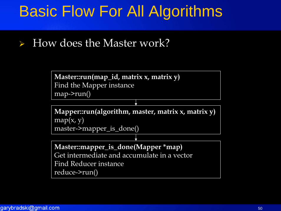
How does the Master work?
Master::run(map_id, matrix x, matrix y)Find the Mapper instancemap->run()
Basic Flow For All Algorithms
Mapper::run(algorithm, master, matrix x, matrix y)map(x, y)master->mapper_is_done()
Master::mapper_is_done(Mapper *map)Get intermediate and accumulate in a vectorFind Reducer instancereduce->run()
51
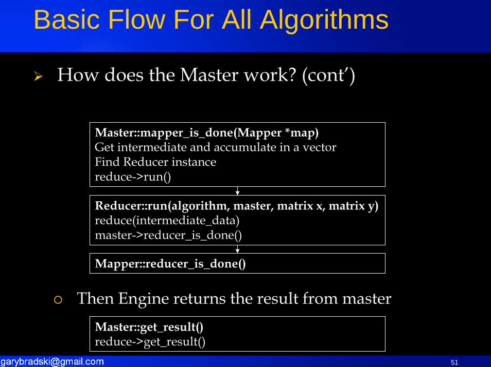
How does the Master work? (cont’)
Reducer::run(algorithm, master, matrix x, matrix y)reduce(intermediate_data)master->reducer_is_done()
Basic Flow For All Algorithms
Mapper::reducer_is_done()
Master::mapper_is_done(Mapper *map)Get intermediate and accumulate in a vectorFind Reducer instancereduce->run()
Master::get_result()reduce->get_result()
Then Engine returns the result from master

52
Where does parallelism takes place
Sequential Code
MAP
REDUCE
Sequential Code

53
A matrix of featuresEach row is one input vector.Each column corresponds to a separate feature.
indicates the i-th row vector
Splitting the input matrixThe input matrix is split into n submatrix, where n is the number of threads.Computation is are on input vectors; only 1-D decomposition is done.
⎟⎟⎟
⎠
⎞
⎜⎜⎜
⎝
⎛
=)2(
2)2(
1)2(
0
)1(2
)1(1
)1(0
)0(2
)0(1
)0(0
xxxxxxxxx
X
)(ix
Input Data

54
ALGORITHM DESCRIPTION

55
Expectation-Maximization AlgorithmFinds maximum likelihood estimates of parameters in probabilistic models.Alternates between expectation (E) step and maximization (M) step.
E step
M step
EM Algorithm
),,;|( )()( Σ== μφiij xjzPw
mwm
ii
jj∑== 1
)(
φ∑∑
=
== m
ii
j
m
iii
jj
w
xw
1)(
1)()(
μ
∑∑
=
=−⋅−⋅
=Σ m
ii
j
m
iT
ji
jii
jj
w
xxw
1)(
1)()()( )()( μμ

56
x, w0, w1x is the input data matrix where columns are featuresw are vectors of probabilities of each row of features to map to a 0 or 1Initially, w0 and w1 are some random values, satisfying w0 j +w1 j =1
class MStepMapper_PHI, class MStepReducer_PHIThe mapper sums w0 j of its portion to produce intermediate data.The reducer takes the partial sums and produces a global sum.
class MStepMapper_MU, class MStepReducer_MUThe mapper obtains mu0 and mu1 by summing w0 j *x j and w1 j *x jrespectively.The reducer takes the partial mu0s and mu1s, and produces a global average mu0, mu1.
class MStepMapper_SIGMA, class MStepReducer_SIGMAThe mapper produces a covariance matrix for each row and sums the covariance matrix to produce a partial sigma.The reducer takes the partial sigma and produces a global sigma.
class EStepMapperEstimates w0 and w1 using the current phi, mu, and sigma values
EM Algorithm Map-Reduce

57
Sequential code – possible parallelizationThe reduce part of the code is executed by only one thread.Reduction can be done in parallel, but this requires change in the current map-reduce structure of the code.
Sequential code – inevitableThere is a part of code where sequential execution is inevitable.Here, matrix LU decomposition is performed to obtain the inverse matrix and determinant of Sigma.This part does not scale with the number of input, but only to the square of the number of features.The maximum number of features with the current sensor data is 120, so it might be better to leave it sequential.
Run on the sequential version of EMExperimented with 1000 rows, 120 features on a Pentium-D machine
EM Algorithm Performance Analysis

58
Run the single thread version of EMExperimented with 100 and 1000 rows, 120 features on a Pentium-DIt was really EStepMapper that took up most of the execution time.The reduction part was barely measureable at all.The LU decomposition and inverse matrix part took a fixed amount of time(~14 sec) and did not change with the number of rows.
EM Algorithm Performance Analysis
59
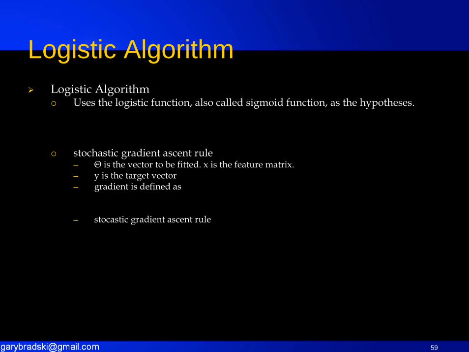
Logistic AlgorithmUses the logistic function, also called sigmoid function, as the hypotheses.
stochastic gradient ascent rule─ Θ is the vector to be fitted. x is the feature matrix.─ y is the target vector─ gradient is defined as
─ stocastic gradient ascent rule
Logistic Algorithm
xT
T
exgxh
θθ θ−+
==1
1)()(
)()()( ))(( iii xxhy ⋅− θ
)()()( ))((: ij
iijj xxhy θαθθ −+=

60
LabelThe label is the target vector which has the same number of rows as the feature matrix.The label was never initialized in this code, and most of any other codes.This can lead to incorrect answers.This shouldn’t, however affect the runtime, and the input feature matrix itself isn’t “valid” data anyways.
Algorithm main loopLoops until tolerance condition is met, or until the number of iteration reaches 10.The tolerance condition is considered to be met when the norm of the gradient is less than 3.The step size for the gradient is given as 0.0001
class LogisticMapperThe mapper sums the gradient value for each row to get a partial sum of gradients.The reducer sums the intermediate gradient values to produce a global gradient.
Logistic Algorithm code

61
Sequential partAfter getting the global gradient, it is scaled, added to the current theta, and is used to compute the norm.All three operations are independent to the number of input data.Thus this part consumes about fixed amount of time, it is not easy to parallelize, and it might not be worth the effort.
Logistic Algorithm code

62
Gaussian Discriminant Analysis modelEssentially finding the maximum likelihood estimates of the parameters.
Almost same as the M step in the EM algorithm.
GDA Algorithm
∑==⋅=
m
i iym 1
}1{11φ
∑∑
=
=
=
⋅== m
ii
m
iii
y
xy
1)(
1)()(
0}0{1
}0{1μ
∑ =−⋅−=Σ
m
iT
yi
yi
ii xxm 1
)()( )()(1)()( μμ
∑∑
=
=
=
⋅== m
ii
m
iii
y
xy
1)(
1)()(
1}1{1
}1{1μ

63
class GDAMapper_PHI, class GDAReducer_PHIThe mapper sums the labels of its portion.The reducer takes the partial sums and produces a global sum.
class GDAMapper_MU, class GDAReducer_MUThe mapper obtains mu0 and mu1 by summing {labelj =0}*xj and {labelj =1}*xjrespectively.The reducer takes the partial mu0s and mu1s, and produces a global average mu0, mu1.
class GDAMapper_SIGMA, class GDAReducer_SIGMAThe mapper produces a covariance matrix for each row and sums the covariance matrix to produce a partial sigma.The reducer takes the partial sigma and produces a global sigma.
Sequential codeSimilar as to the EM algorithm, the size of the sequential part is fixed to the number of columns (i.e. features).
GDA Algorithm code

64
K-means AlgorithmA variant of the EM algorithm.Clusters objects based on attributes into k partitions.The objective is to minimize total intra-cluster variance.
Here, μ is the centroid, or mean point of all the points
K-means Algorithm
∑ ∑=∈
−=k
iSj
iji
xV1
2|| μ
ij Sx ∈

65
centroidInitially some dummy value (the first k rows of the feature matrix)Gets updated while running the algorithm in multiple iterations
class KMeansMapperThe mapper places each row to a cluster by its similarity to the centroid.The similarity is measured by the dot-product between the input row vector and the centroid vector.The feature row vector is sent to the cluster of which centroid showed the maximum similarity.
class KMeansReducerThe reducer accumulates each centroid with input vectors in the same cluster.The centroid is scaled down by the number of elements in the cluster, makingthe centroid the mean of the input vectors.This part of the code is executed by only one thread.However, the reduce runtime is only 1% of the map runtime.Parallelizing this part would need either a lock, or private centroids with additional reduction, which means overhead.
K-means Algorithm code

66
Naive Bayes AlgorithmBased on the assumption that xi’s condition is independent of y.Discretizes the data in this implementation into 8 categories.To make a prediction, just compute
NB Algorithm
)1())1|(()0())0|((
)1())1|((
)()1()1|()|1(
11
1
==+==
===
====
∏∏∏
==
=
ypyxpypyxp
ypyxp
xpypyxpxyp
n
i in
i i
n
i i

67
DiscretizationBefore running the algorithm, the input is discretized into 8 categories per column (i.e. feature).
class NB_MapperThe mapper counts the number of occurrence per category per column, once given y=0 and once given y=1.Stores the counted data for each category in a 8x2 matrix called “table” for that column.
class NB_ReducerGets the intermediate data and sums them into one 8x2 matrix.Stores the “probability” per category for each column.
NB Algorithm source code

68
Principle Component AnalysisOnly requires eigenvector computations.The problem is essentially maximizing the following value with a unit length u:
This gives the principle eigenvector of is the covariance matrix.
PCA Algorithm
uxxm
uuxm
m
iTiiTm
ii )1()(1
1)()(
12)( ∑∑ ===
∑ =
m
iTii xx
m 1)()(1
69
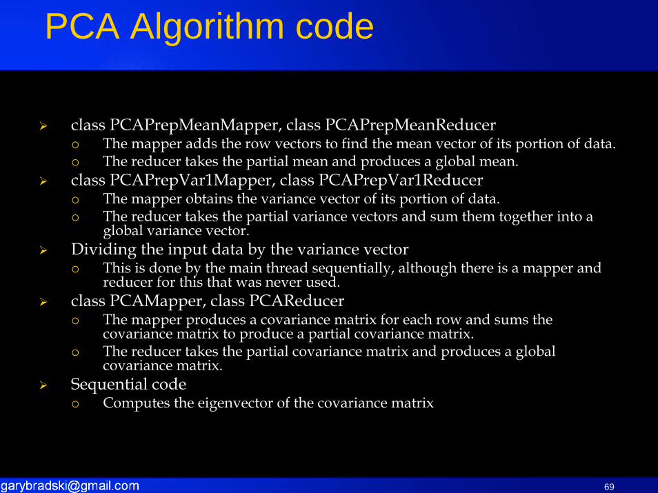
class PCAPrepMeanMapper, class PCAPrepMeanReducerThe mapper adds the row vectors to find the mean vector of its portion of data.The reducer takes the partial mean and produces a global mean.
class PCAPrepVar1Mapper, class PCAPrepVar1ReducerThe mapper obtains the variance vector of its portion of data.The reducer takes the partial variance vectors and sum them together into a global variance vector.
Dividing the input data by the variance vectorThis is done by the main thread sequentially, although there is a mapper and reducer for this that was never used.
class PCAMapper, class PCAReducerThe mapper produces a covariance matrix for each row and sums the covariance matrix to produce a partial covariance matrix.The reducer takes the partial covariance matrix and produces a global covariance matrix.
Sequential codeComputes the eigenvector of the covariance matrix
PCA Algorithm code

70
Independent Component AnalysisA computational method for separating a multivariate signal into additive subcomponents supposing the mutual statistical independence of the non-Gaussian source.This is the case where there is a source vector that is generated from independent sources, and our goal is to recover the sources.
Let . Our goal is to find W so that we can recover the sources.W is obtained and updated by iteratively computing the following rule:
g is the sigmoid function and alpha is the learning rate.
1−= AW
Asx
ICA Algorithm
=
⎟⎟⎟⎟
⎠
⎞
⎜⎜⎜⎜
⎝
⎛
+⎥⎥⎥
⎦
⎤
⎢⎢⎢
⎣
⎡
−
−+= −1)(
)(
)(1
)()(21
)(21: TTi
iTn
iT
Wxxwg
xwgWW Mα

71
class ICAMapper, class ICAReducerThe mapper computes the part of the gradient and sums them to create a partial gradient.The reducer takes the partial gradient and sums them to a global gradient.
Computing the invert matrix of WThis part is done in serial.W is only dependent on the number of features, so the computation time of this part is fixed to the square of the number of features.The main thread performs the LU decomposition and computes the transpose invert matrix of W.This is added to the gradient and the gradient is scaled by the learning rate.
W is computed and updated for 10 iterations.
ICA Algorithm code
[ ] )(1 )(21 iT xwg ⋅−

72
LWLR AlgorithmMight stand for “locally weighted linear regression”, but I’m not sure.Get A matrix and b vector, then solve the linear equation to get theta.
The weight vector for this code is all 1s, which does not matter since it does not affect the performance.
xxwarraymultA T ⋅= ),(
LWLR Algorithm
r
)( ij
ijjj xywb ∑=
bA =⋅θ

73
class LWLR_A_Mapper, class LWLR_A_ReducerThe mapper computes the partial A matrix for its portion of data.The reducer sums the partial A matrix to create a global A matrix.
class LWLR_B_Mapper, class LWLR_B_ReducerThe mapper computes the partial b vector for its portion of data.The reducer sums the partial b vector to create a global b vector.
Householder solver for linear algebraThis part is serial, executed by the main thread.The main thread uses householder solver to solve the linear equation.Both the size of A and b is independent of the number of inputs. Therefore the computation time for this part is fixed.
LWLR Algorithm code