
Manual2130ProEn.pdf
360
Reference Manual CSI 2130 Machinery Health™ Analyzer Single- and Dual-Channel MHM-97017.13 Copyright
-
Upload
demostenes69 -
Category
Documents
-
view
54 -
download
2
Transcript of Manual2130ProEn.pdf
Reference Manual
CSI 2130 Machinery Health™ Analyzer
Single- and Dual-Channel
MHM-97017.13 Copyright

© 2011 by Emerson Process Management.All rights reserved.
No part of this publication may be reproduced, trans-mitted, transcribed, stored in a retrieval system, or translated into any language in any form by any means without the written permission of Emerson.
DisclaimerThis manual is provided for informational purposes. COMPUTATIONAL SYSTEMS, INCORPORATED MAKES NO WARRANTY OF ANY KIND WITH REGARD TO THIS MATERIAL, INCLUDING, BUT NOT LIMITED TO, THE IMPLIED WARRANTIES OF MERCHANTABILITY AND FIT-NESS FOR A PARTICULAR PURPOSE. Computational Systems, Incorporated shall not be liable for errors, omissions, or inconsistencies that may be contained herein or for incidental or consequential damages in connection with the furnishing, performance, or use of this material. Information in this document is sub-ject to change without notice and does not represent a commitment on the part of Computational Sys-tems, Incorporated. The information in this manual is not all-inclusive and cannot cover all unique situ-ations.
Product SupportShould you have any comments on this documenta-tion or questions concerning the Agreement on the following pages, please contact Emerson’s Product Support Department.
Address:Emerson Process Management835 Innovation DriveKnoxville, TN 37932 USA
Phone:United States and Canada: 865-675-4274
FAX:865-218-1416
Internet E-mail:United States and Canada:
Worldwide Web:http://www.MHM.Assetweb.com
Emerson Process Management’s Reference ManualsThis document was written, illustrated, and pro-duced by Emerson’s Engineering Publications Group using Adobe™ FrameMaker®, Adobe Photo-Shop®, and Macromedia® FreeHand™. Printed copies are produced using the Xerox™ DocuTech™ pub-lishing system.
Trademarks and ServicemarksAccuTrend; Changing the way the world performs maintenance, and Emerson Process Management logo; CSIRBM‚(Mexico); Doctor Know; Infranalysis; InfraRoute; Levels of Awareness Training; M&D; MachineGuard; MachineView; MasterNet; Motor-View; Nspectr; O&M Workstation; OilView (Japan); RBMware; Reliability-Based Maintenance, and logo; RollView; StarterTrend; STATUS Tech-nologies; TrendSetter; Tribology Minilab; UltrasSpec; WAVEPAK; and RBMconsultant are registered trademarks of Emerson Process Manage-ment.
CSI (China, Japan, Venezuela, Australia); CSIRBM (Venezuela); Status Condition Monitor; PeakVue; RBMview; RBMware (Australia, China, Japan); RBMwizard; Reliability-Based Maintenance (Vene-zuela); SonicScan; SonicView; SST; STATUS RF SmartSensor; STATUS RF Transceiver; VersaBal; VibPro; VibView; and Weldwatch are pending trademarks of Computational Systems, Incorpo-rated.
Lubricant Profile and Trivector are registered ser-vicemarks of Computational Systems, Incorporated.
RBM; RBMware (China); Reliability-Based Mainte-nance (Venezuela); and STATUS Technologies and design are pending servicemarks of Computational Systems, Incorporated.
Adobe is a trademark and FrameMaker and Photo-Shop are registered trademarks of Adobe Systems, Inc. Power Macintosh is a trademark of Apple Com-puter, Inc. Macromedia is a registered trademark and FreeHand is a trademark of Macromedia, Inc. Xerox and DocuTech are trademarks of Xerox Corporation.
All other brand or product names are trademarks or registered trademarks of their respective companies.
2

PatentsThe product(s) described in this manual are covered under existing and pending patents.
License Agreement
IMPORTANT: CAREFULLY READ ALL THE TERMS AND CONDITIONS OF THIS AGREEMENT BEFORE OPENING THE PACKAGE OR PROCEEDING WITH INSTALLATION. OPENING THE PACKAGE OR COMPLETING THE INSTAL-LATION INDICATES YOUR ACCEPTANCE OF THE TERMS AND CONDITIONS CONTAINED IN THIS AGREEMENT.
IF YOU DO NOT AGREE TO THE TERMS AND CONDI-TIONS CONTAINED IN THIS AGREEMENT, CANCEL ANY INSTALLATION AND PROMPTLY RETURN THIS PRODUCT AND THE ASSOCIATED DOCUMENTATION TO EMERSON PROCESS MANAGEMENT, AND YOUR MONEY WILL BE REFUNDED. NO REFUNDS WILL BE GIVEN FOR PROD-UCTS WITH DAMAGED OR MISSING COMPONENTS.
Definition of SoftwareAs used herein, software refers to any computer pro-gram contained on any medium. Software includes downloadable firmware for use in devices such as analyzers or MotorStatus units and it includes com-puter programs executable on computers or com-puter networks.
Software LicenseYou have the non-exclusive right to use this soft-ware on only one device at a time. You may back-up the software for archival purposes. For network sys-tems, you have the non-exclusive right to install this software on only one server. Read/write access is limited to the number of licenses purchased. The number of read-only accesses is not limited.
Software UpdatesEmerson Process Management agrees to provide Purchaser, at no charge except for media, prepara-tion and shipping charges, for one (1) year from the date of purchase, updates to the software made at the sole discretion of Emerson. Should Purchaser desire to purchase software maintenance for the next suc-ceeding year following the first year from the date of purchase, and thereafter on an annual basis, and if Emerson Process Management is still providing maintenance, Purchaser may purchase the same, annually, at the existing rate.
Updates/UpgradesUpon receipt of new Emerson Process Management software replacing older Emerson software, you have 30 days to install and test the new Emerson software on the same or a different device. At the end of the 30-day test period, you must both remove and return the new Emerson software or remove the older Emerson Process Management software.
OwnershipThe licensed software and all derivatives are the sole property of Emerson Process Management Tech-nology, Inc. You may not disassemble, decompile, reverse engineer or otherwise translate the licensed program. You may not distribute copies of the pro-gram or documentation, in whole or in part, to another party. You may not in any way distort, or otherwise modify the program or any part of the doc-umentation without prior written consent from Emerson Process Management.
TransferYou may transfer the software and license to another party only with the written consent of Emerson Pro-cess Management and only if the other party agrees to accept the terms and conditions of this Agree-ment. If you transfer the program, you must transfer the documentation and any backup copies or transfer only the documentation and destroy any backup copies.
CopyrightThe software and documentation are copyrighted. All rights are reserved.
TerminationIf you commit a material breach of this Agreement, Emerson Process Management may terminate the Agreement by written notice.
Virus DisclaimerEmerson Process Management uses the latest virus checking technologies to test all its software. How-ever, since no anti-virus system is 100% reliable, we strongly advise that you use and anti-virus system in which have confidence to verify the software is virus-free. Emerson makes no representations or warranties to the effect that the licensed software is virus-free.
3

NO WARRANTYTHE PROGRAM IS PROVIDED “AS-IS” WITHOUT ANY WARRANTIES, EXPRESS OR IMPLIED, INCLUDING BUT NOT LIMITED TO ANY WARRANTIES OR MERCHANT-ABILITY OR FITNESS FOR A PARTICULAR PURPOSE.
LIMITATION OF LIABILITY AND REMEDIESIN NO EVENT WILL EMERSON PROCESS MANAGEMENT BE LIABLE TO YOU OR ANY THIRD PARTY FOR ANY DAM-AGES, INCLUDING ANY LOST PROFITS, LOST SAVINGS, OR OTHER INCIDENTAL OR CONSEQUENTIAL DAMAGES ARISING OUT OF THE USE OR THE INABILITY TO USE THIS PROGRAM. THE LICENSEE'S SOLE AND EXCLUSIVE REMEDY IN THE EVENT OF A DEFECT IN WORKMANSHIP OR MATERIAL IS EXPRESSLY LIMITED TO THE REPLACE-MENT OF THE DISKETTES. IN NO EVENT WILL EMERSON PROCESS MANAGEMENT'S LIABILITY EXCEED THE PUR-CHASE PRICE OF THE PRODUCT.
Export RestrictionsYou agree to comply fully with all laws, regulations, decrees and orders of the Unites States of America that restrict or prohibit the exportation (or reexpor-tation) of technical data and/or the direct product of it to other countries, including, without limitation, the U.S. Export Administration Regulations.
U.S. Government RightsThe programs and related materials are provided with “RESTRICTED RIGHTS”. Use, duplication or disclosure by the U.S. Government is subject to restrictions set forth in the Federal Acquisition Reg-ulations and its Supplements.
Hardware Technical Help1. Please have the number of the current version of your firmware ready when you call. The version of the firmware in Emerson Process Management’s Model 2100 series, Model 2400, and other analyzers appears on the power-up screen that is displayed when the analyzer is turned on.
2. If you have a problem, explain the exact nature of your problem. For example, what are the error mes-sages? When to they occur? Know what you were doing when the problem occurred. For example, what mode were you in? What steps did you go through? Try to determine before you call whether the problem is repeatable.
Hardware Repair Emerson repairs and updates its hardware products free for one year from the date of purchase. This ser-vice warranty includes hardware improvement, mod-ification, correction, recalibration, update, and maintenance for normal wear. This service warranty excludes repair of damage from misuse, abuse, neglect, carelessness, or modification performed by anyone other than Emerson Process Management.
After the one year service warranty expires, each return of a Emerson Process Management hardware product is subject to a minimum service fee. If the cost of repair exceeds this minimum fee, we will call you with an estimate before performing any work. Contact Emerson Process Management’s Product Support Department for information concerning the current rates.
Returning Items
1. Call Product Support (see page 2) to obtain a return authorization number. Please write it clearly and prominently on the outside of the shipping container..
2. If returning for credit, return all accessories originally shipped with the item(s). Include cables, software diskettes, manuals, etc.
3. Enclose a note that describes the reason(s) you are returning the item(s).
4. Insure your package for return shipment. Shipping costs and any losses during shipment are your responsibility. COD packages cannot be accepted and will be returned unopened.
Obsolete HardwareAlthough Emerson Process Management will honor all contractual agreements and will make every effort to ensure that its software packages are “back-ward compatible,” to take advantage of advances in newer hardware platforms and to keep our programs reasonably small, Emerson reserves the right to dis-continue support for old or out-of-date hardware items.
4
Software Technical Help
Software Technical SupportEmerson Process Management provides technical support through the following for those under main-tenance contracts:
• Telephone assistantance and communication via the Internet.
• Mass updates that are released during that time.• Interim updates upon request. Please contact Emerson
Process Management Customer Services for more information.
CE NoticeEmerson Process Management products bearing the
symbol on the product or in the user’s manual are in compliance with applicable EMC and Safety Directives of the European Union. In accordance with CENELEC standard EN 50082-2, normal intended operation is specified as follows:
1. The product must not pose a safety hazard.2. The product must not sustain damage as a result of use
under environmental conditions specified in the user documentation.
3. The product must stay in or default to an operating mode that is restorable by the user.
4. The product must not lose program memory, user-configured memory (e.g., routes), or previously stored data memory. When apparent, the user may need to initiate a reset and/or restart of a data acquisition in progress.
A Declaration of Conformity certificate for the product is on file at the appropriate Emerson Process Management office within the European Commu-nity.
5

6

Contents
Chapter 1 • Introduction to the CSI 2130
Special Text . . . . . . . . . . . . . . . . . . . . . . . . . . . . . . . . . . . . . . . . . . . . . . . . . . . . . . . . . . . . . . . . 1-1Precautions . . . . . . . . . . . . . . . . . . . . . . . . . . . . . . . . . . . . . . . . . . . . . . . . . . . . . . . . . . . . . . . . . 1-2Single- and Dual-Channel Versions of the CSI 2130. . . . . . . . . . . . . . . . . . . . . . . . . 1-4Standard Equipment and Options. . . . . . . . . . . . . . . . . . . . . . . . . . . . . . . . . . . . . . . . . . . . 1-5
Accessories – supplied . . . . . . . . . . . . . . . . . . . . . . . . . . . . . . . . . . . . . . . . . . . . . . . . . . . . . 1-5Machinery Health Manager Software Version Prerequisites . . . . . . . . . . . . . . . . . . . . . . . . . . . . . . . . . . . . . . . . . . . . . . . . . . . . . . . . . . . . . . . . 1-7Unpacking the CSI 2130 . . . . . . . . . . . . . . . . . . . . . . . . . . . . . . . . . . . . . . . . . . . . . . . . . . . . 1-8Front Panel: Buttons, Indicators, and Keys . . . . . . . . . . . . . . . . . . . . . . . . . . . . . . . . . 1-16Battery Use and Care . . . . . . . . . . . . . . . . . . . . . . . . . . . . . . . . . . . . . . . . . . . . . . . . . . . . . . 1-18
To look at both the battery charge and voltage levels . . . . . . . . . . . . . . . . . . . . . . . . . . 1-19Battery Discharge (CSI 2130 with Ethernet port and SD slot only) . . . . . . . . . . . . . . 1-23LED for Charging . . . . . . . . . . . . . . . . . . . . . . . . . . . . . . . . . . . . . . . . . . . . . . . . . . . . . . . . 1-26Recharging the Battery Pack . . . . . . . . . . . . . . . . . . . . . . . . . . . . . . . . . . . . . . . . . . . . . . . 1-27Changing the Battery . . . . . . . . . . . . . . . . . . . . . . . . . . . . . . . . . . . . . . . . . . . . . . . . . . . . . 1-28
Chapter 2 • Shell Program Overview
The CSI 2130 Shell. . . . . . . . . . . . . . . . . . . . . . . . . . . . . . . . . . . . . . . . . . . . . . . . . . . . . . . . 2-1Analyze and Advanced Analyze. . . . . . . . . . . . . . . . . . . . . . . . . . . . . . . . . . . . . . . . . . . . . 2-2
Basic Setup . . . . . . . . . . . . . . . . . . . . . . . . . . . . . . . . . . . . . . . . . . . . . . . . . . . . . . . . . . . . . . . . . 2-3File Utility. . . . . . . . . . . . . . . . . . . . . . . . . . . . . . . . . . . . . . . . . . . . . . . . . . . . . . . . . . . . . . . . 2-3Set Display Units. . . . . . . . . . . . . . . . . . . . . . . . . . . . . . . . . . . . . . . . . . . . . . . . . . . . . . . . . 2-10Communications Setup . . . . . . . . . . . . . . . . . . . . . . . . . . . . . . . . . . . . . . . . . . . . . . . . . . . 2-13Program Manager . . . . . . . . . . . . . . . . . . . . . . . . . . . . . . . . . . . . . . . . . . . . . . . . . . . . . . . . 2-23How do I ... Add a Program?. . . . . . . . . . . . . . . . . . . . . . . . . . . . . . . . . . . . . . . . . . . . . . . 2-24How do I ... Update the Base Firmware?. . . . . . . . . . . . . . . . . . . . . . . . . . . . . . . . . . . . . 2-29How do I .. Delete a Program? . . . . . . . . . . . . . . . . . . . . . . . . . . . . . . . . . . . . . . . . . . . . . 2-32How do I... Load a New Splash Screen?. . . . . . . . . . . . . . . . . . . . . . . . . . . . . . . . . . . . . 2-33
ALT: Alternate Screens . . . . . . . . . . . . . . . . . . . . . . . . . . . . . . . . . . . . . . . . . . . . . . . . . . . . 2-36ALT Screen . . . . . . . . . . . . . . . . . . . . . . . . . . . . . . . . . . . . . . . . . . . . . . . . . . . . . . . . . . . . . 2-36Version Information . . . . . . . . . . . . . . . . . . . . . . . . . . . . . . . . . . . . . . . . . . . . . . . . . . . . . . 2-37General Setup. . . . . . . . . . . . . . . . . . . . . . . . . . . . . . . . . . . . . . . . . . . . . . . . . . . . . . . . . . . . 2-38Setting Time. . . . . . . . . . . . . . . . . . . . . . . . . . . . . . . . . . . . . . . . . . . . . . . . . . . . . . . . . . . . . 2-42
7
Memory Utility. . . . . . . . . . . . . . . . . . . . . . . . . . . . . . . . . . . . . . . . . . . . . . . . . . . . . . . . . . . 2-45View Error Log . . . . . . . . . . . . . . . . . . . . . . . . . . . . . . . . . . . . . . . . . . . . . . . . . . . . . . . . . . 2-47Connect For Printing . . . . . . . . . . . . . . . . . . . . . . . . . . . . . . . . . . . . . . . . . . . . . . . . . . . . . . 2-48
Chapter 3 • Data Transfer
Overview . . . . . . . . . . . . . . . . . . . . . . . . . . . . . . . . . . . . . . . . . . . . . . . . . . . . . . . . . . . . . . . . . . . 3-1Data Transfer Host . . . . . . . . . . . . . . . . . . . . . . . . . . . . . . . . . . . . . . . . . . . . . . . . . . . . . . . . . . 3-3
The Navigator. . . . . . . . . . . . . . . . . . . . . . . . . . . . . . . . . . . . . . . . . . . . . . . . . . . . . . . . . . . . . 3-4Device(s) Waiting For Connection List . . . . . . . . . . . . . . . . . . . . . . . . . . . . . . . . . . . . . . . 3-4
CSI 2130 Setup . . . . . . . . . . . . . . . . . . . . . . . . . . . . . . . . . . . . . . . . . . . . . . . . . . . . . . . . . . . . . 3-5Installing the USB Driver . . . . . . . . . . . . . . . . . . . . . . . . . . . . . . . . . . . . . . . . . . . . . . . . . . . 3-6Route Overrides . . . . . . . . . . . . . . . . . . . . . . . . . . . . . . . . . . . . . . . . . . . . . . . . . . . . . . . . . . 3-14CSI 2130 Route Setup. . . . . . . . . . . . . . . . . . . . . . . . . . . . . . . . . . . . . . . . . . . . . . . . . . . . . 3-16
CSI 2130 Printing . . . . . . . . . . . . . . . . . . . . . . . . . . . . . . . . . . . . . . . . . . . . . . . . . . . . . . . . . . 3-23Screen Captures . . . . . . . . . . . . . . . . . . . . . . . . . . . . . . . . . . . . . . . . . . . . . . . . . . . . . . . . . . 3-26CSI 2130 Offline Printing. . . . . . . . . . . . . . . . . . . . . . . . . . . . . . . . . . . . . . . . . . . . . . . . . . 3-26
Standalone Data Transfer Application . . . . . . . . . . . . . . . . . . . . . . . . . . . . . . . . . . . . . . 3-27
Chapter 4 • Cables and Adapters
Compatibility with the CSI 2130 . . . . . . . . . . . . . . . . . . . . . . . . . . . . . . . . . . . . . . . . . . . . 4-1Optional Accessories for the CSI 2130. . . . . . . . . . . . . . . . . . . . . . . . . . . . . . . . . . . . . . . . 4-3
Chapter 5 • Route
What is a Route? . . . . . . . . . . . . . . . . . . . . . . . . . . . . . . . . . . . . . . . . . . . . . . . . . . . . . . . . . . 5-1Route Tips. . . . . . . . . . . . . . . . . . . . . . . . . . . . . . . . . . . . . . . . . . . . . . . . . . . . . . . . . . . . . . . . 5-1
Using a Route . . . . . . . . . . . . . . . . . . . . . . . . . . . . . . . . . . . . . . . . . . . . . . . . . . . . . . . . . . . . . . . 5-2Collecting Data. . . . . . . . . . . . . . . . . . . . . . . . . . . . . . . . . . . . . . . . . . . . . . . . . . . . . . . . . . . . 5-2
Route Data Collection . . . . . . . . . . . . . . . . . . . . . . . . . . . . . . . . . . . . . . . . . . . . . . . . . . . . . . . 5-6Route Data Collection: Measurement Point Display . . . . . . . . . . . . . . . . . . . . . . . . . . . . 5-8Route Data Collection: Keys and Functions . . . . . . . . . . . . . . . . . . . . . . . . . . . . . . . . . . 5-11Alt Route Data Collection: Keys and Functions. . . . . . . . . . . . . . . . . . . . . . . . . . . . . . . 5-19
Notes . . . . . . . . . . . . . . . . . . . . . . . . . . . . . . . . . . . . . . . . . . . . . . . . . . . . . . . . . . . . . . . . . . . . . . 5-38Add Notes . . . . . . . . . . . . . . . . . . . . . . . . . . . . . . . . . . . . . . . . . . . . . . . . . . . . . . . . . . . . . . . 5-38How Do I ... Use Notes?. . . . . . . . . . . . . . . . . . . . . . . . . . . . . . . . . . . . . . . . . . . . . . . . . . . 5-41
Downloading Routes and Uploading Data . . . . . . . . . . . . . . . . . . . . . . . . . . . . . . . . . . 5-42How do I ... Load a Route for the First Time?. . . . . . . . . . . . . . . . . . . . . . . . . . . . . . . . . 5-42
8

Multiple Route Load for CSI 2130. . . . . . . . . . . . . . . . . . . . . . . . . . . . . . . . . . . . . . . . . . 5-45Time Discrepancy. . . . . . . . . . . . . . . . . . . . . . . . . . . . . . . . . . . . . . . . . . . . . . . . . . . . . . . . 5-48
Chapter 6 • Analysis Experts
Running the Experts . . . . . . . . . . . . . . . . . . . . . . . . . . . . . . . . . . . . . . . . . . . . . . . . . . . . . . . . 6-1Analysis Experts . . . . . . . . . . . . . . . . . . . . . . . . . . . . . . . . . . . . . . . . . . . . . . . . . . . . . . . . . . 6-2Using Analysis Experts . . . . . . . . . . . . . . . . . . . . . . . . . . . . . . . . . . . . . . . . . . . . . . . . . . . 6-14
Chapter 7 • Analyze
Using Analyze . . . . . . . . . . . . . . . . . . . . . . . . . . . . . . . . . . . . . . . . . . . . . . . . . . . . . . . . . . . . . . 7-1Manual Analyze . . . . . . . . . . . . . . . . . . . . . . . . . . . . . . . . . . . . . . . . . . . . . . . . . . . . . . . . . . . . 7-9
Special Features. . . . . . . . . . . . . . . . . . . . . . . . . . . . . . . . . . . . . . . . . . . . . . . . . . . . . . . . . . 7-11Spectra. . . . . . . . . . . . . . . . . . . . . . . . . . . . . . . . . . . . . . . . . . . . . . . . . . . . . . . . . . . . . . . . . . 7-17Waveform. . . . . . . . . . . . . . . . . . . . . . . . . . . . . . . . . . . . . . . . . . . . . . . . . . . . . . . . . . . . . . . 7-22Overall. . . . . . . . . . . . . . . . . . . . . . . . . . . . . . . . . . . . . . . . . . . . . . . . . . . . . . . . . . . . . . . . . . 7-24DC Volts and Temperature . . . . . . . . . . . . . . . . . . . . . . . . . . . . . . . . . . . . . . . . . . . . . . . . 7-25Third Octave. . . . . . . . . . . . . . . . . . . . . . . . . . . . . . . . . . . . . . . . . . . . . . . . . . . . . . . . . . . . . 7-27True Zoom and Zoom Analysis . . . . . . . . . . . . . . . . . . . . . . . . . . . . . . . . . . . . . . . . . . . . 7-29Cascade. . . . . . . . . . . . . . . . . . . . . . . . . . . . . . . . . . . . . . . . . . . . . . . . . . . . . . . . . . . . . . . . . 7-31Peak and Phase. . . . . . . . . . . . . . . . . . . . . . . . . . . . . . . . . . . . . . . . . . . . . . . . . . . . . . . . . . . 7-37Filtered Orbit . . . . . . . . . . . . . . . . . . . . . . . . . . . . . . . . . . . . . . . . . . . . . . . . . . . . . . . . . . . . 7-39Cross Channel Phase. . . . . . . . . . . . . . . . . . . . . . . . . . . . . . . . . . . . . . . . . . . . . . . . . . . . . . 7-42
Plot Functions . . . . . . . . . . . . . . . . . . . . . . . . . . . . . . . . . . . . . . . . . . . . . . . . . . . . . . . . . . . . . 7-44Special Plot Keys. . . . . . . . . . . . . . . . . . . . . . . . . . . . . . . . . . . . . . . . . . . . . . . . . . . . . . . . . 7-53Auto Correlation . . . . . . . . . . . . . . . . . . . . . . . . . . . . . . . . . . . . . . . . . . . . . . . . . . . . . . . . . 7-56
Job . . . . . . . . . . . . . . . . . . . . . . . . . . . . . . . . . . . . . . . . . . . . . . . . . . . . . . . . . . . . . . . . . . . . . . . . 7-59Connect for Transfer: Dumping Jobs. . . . . . . . . . . . . . . . . . . . . . . . . . . . . . . . . . . . . . . . 7-62
Chapter 8 • Advanced Analyze Functions
Analyze Mode . . . . . . . . . . . . . . . . . . . . . . . . . . . . . . . . . . . . . . . . . . . . . . . . . . . . . . . . . . . . 8-2Impact testing. . . . . . . . . . . . . . . . . . . . . . . . . . . . . . . . . . . . . . . . . . . . . . . . . . . . . . . . . . . . . . . 8-3
Analyze Setup for Impact Mode. . . . . . . . . . . . . . . . . . . . . . . . . . . . . . . . . . . . . . . . . . . . . 8-4Input Setup . . . . . . . . . . . . . . . . . . . . . . . . . . . . . . . . . . . . . . . . . . . . . . . . . . . . . . . . . . . . . . . 8-7Impact Acquisition Process . . . . . . . . . . . . . . . . . . . . . . . . . . . . . . . . . . . . . . . . . . . . . . . . 8-10Impact Waveform Plots . . . . . . . . . . . . . . . . . . . . . . . . . . . . . . . . . . . . . . . . . . . . . . . . . . . 8-11
Advanced Cross Channel Testing . . . . . . . . . . . . . . . . . . . . . . . . . . . . . . . . . . . . . . . . . . 8-13Analyze Setup . . . . . . . . . . . . . . . . . . . . . . . . . . . . . . . . . . . . . . . . . . . . . . . . . . . . . . . . . . . 8-14
9
Input Setup . . . . . . . . . . . . . . . . . . . . . . . . . . . . . . . . . . . . . . . . . . . . . . . . . . . . . . . . . . . . . . 8-15Two Channel Plot Setup. . . . . . . . . . . . . . . . . . . . . . . . . . . . . . . . . . . . . . . . . . . . . . . . . . . . 8-16
Plot Setups-Data Plot Setup . . . . . . . . . . . . . . . . . . . . . . . . . . . . . . . . . . . . . . . . . . . . . . . . 8-19Plot Setups-Live Plot Setup . . . . . . . . . . . . . . . . . . . . . . . . . . . . . . . . . . . . . . . . . . . . . . . . 8-21
Applications and Insights Related to Impact Testing . . . . . . . . . . . . . . . . . . . . . . . . 8-22Understanding Impact Testing. . . . . . . . . . . . . . . . . . . . . . . . . . . . . . . . . . . . . . . . . . . . . . 8-23Preliminary Testing Considerations . . . . . . . . . . . . . . . . . . . . . . . . . . . . . . . . . . . . . . . . . 8-30Summary. . . . . . . . . . . . . . . . . . . . . . . . . . . . . . . . . . . . . . . . . . . . . . . . . . . . . . . . . . . . . . . . 8-34
Chapter 9 • Advanced Transient
What is Advanced Transient?. . . . . . . . . . . . . . . . . . . . . . . . . . . . . . . . . . . . . . . . . . . . . . . . 9-1
Chapter 10 • ODS Modal
What is an Operating Deflection Shape? . . . . . . . . . . . . . . . . . . . . . . . . . . . . . . . . . . . . 10-1CSI 2130 ODS Modal Downloadable. . . . . . . . . . . . . . . . . . . . . . . . . . . . . . . . . . . . . . . 10-3
Appendix A • Technical Specifications
Hardware Specifications. . . . . . . . . . . . . . . . . . . . . . . . . . . . . . . . . . . . . . . . . . . . . . . . . . . .A-1Input Specifications . . . . . . . . . . . . . . . . . . . . . . . . . . . . . . . . . . . . . . . . . . . . . . . . . . . . . . . .A-2Measurement Specifications . . . . . . . . . . . . . . . . . . . . . . . . . . . . . . . . . . . . . . . . . . . . . . . .A-5Output . . . . . . . . . . . . . . . . . . . . . . . . . . . . . . . . . . . . . . . . . . . . . . . . . . . . . . . . . . . . . . . . . . .A-7
Glossary
Index
10

Chapter 1
Introduction to the CSI 2130
Special TextThe following conventions are used throughout this manual to call special attention to the associated text:
NoteA note paragraph contains special comments or instructions.
Caution!A caution paragraph alerts you to actions that may have a major impact on the equipment, stored data, etc.
A warning paragraph alerts you to actions that may have extremely serious consequences for equipment and/or personnel.
1-1
PrecautionsAny product damage due to these conditions may void the warranty.
Do not change the battery pack with the battery charger connected, damage may occur to the analyzer.
Use only Emerson-approved battery packs.
Use only Emerson-supplied battery chargers approved for use with the CSI 2130 Machinery Health Analyzer. The use of any other charger will most likely damage the analyzer.
Do not use Emerson battery chargers with anything other than their corre-sponding CSI product.
Do not connect a signal larger than +/- 21 volts into the input of the analyzer.
Caution!Emerson does not warrant compatibility or fitness for applica-tion of this product with any device not specifically recom-mended in the product literature.
Caution!Marking for the Waste of Electrical and Electronic Equipment in accordance with Article 11(2) of Directive 2002/96/EC (WEEE) The European Directive 2002/96/EC requires marking:
• That applies to electrical and electronic equipment falling under Annex IA of Directive 2002/96/EC.
• That serves to clearly identify the producer of the equipment and that the equipment has been put on the marker after 13 August 2005
• That the crossed out wheeled bin alerts the end-user to dispose this equipment via the special recycling procedure for electrical/elec-tronic equipment that is applicable in the country of use.
1-2 Introduction to the CSI 2130
• The shown marking is attached to the product and identifies the product to fall within the scope of this Directive.
Warning!Cleaning Instructions: Clean only in a non-hazardous area. Elec-trostatic Hazards. Wipe only with damp cloth.
1-3Precautions
Single- and Dual-Channel Versions of the CSI 2130This manual contains information about multiple options available for the CSI 2130 including a single and dual channel version. The unit can also be purchased with different configurations of applications including Route, Analyze, Advanced Analyze, Balancing, Alignment, and others. Not all applications and features described in this manual apply to all versions of the CSI 2130.
1-4 Introduction to the CSI 2130
Standard Equipment and Options
Accessories – supplied
The CSI 2130 comes with some supplied pieces of equipment and some addi-tional accessories that can be purchased separately.
Standard Equipment• CSI 2130 analyzer• hand straps (two)• shoulder strap with pad• hand pads (two)
Typical accessories for vibration and balancing packages may include the follow-ing:
Accelerometer coiled cable (Turck to 2-pin mil)
General purpose accelerometer
Dual rail magnet
Straight cable (blue, BNC to 2-pin mil)
Straight cable (red, BNC to 2-pin mil)
Dual channel adapter (dual BNC or dual Turck inputs)
Optional Accessories:Triaxial Turck cable
(If using the 2120 25-pin triax cable, please note that the channels will reg-ister in an alternate order.)
404 Tach input cable (Turck to 404 connector, 6.56-ft long, signal and power wires)
BNC Tach input cable (Turck to BNC connector)
18-in. SpeedVue cable
6-ft SpeedVue cable
1-5Standard Equipment and Options

2130 2-channel volts adapter
1-channel accel input cable (Turck to BNC connector)
1-channel volts input cable (Turck to BNC connector)
VGA adapter cable for external display (under battery door)
NoteCSI 2130 won’t support: Shaft Probe, 339 thickness gauge.
NoteCSI 2120 buffered volts input adapters won't work with CSI 2130, buffering is done internally by the analyzer.
NoteThe 648 mux adapter channels will be shifted around, but the balance program will handle this transparently for the existing adapter.
1-6 Introduction to the CSI 2130

Machinery Health Manager Software Version Prerequisites
NoteYour AMS Machinery Manager software and CSI 2130 Machinery Health Analyzer must have compatible software.
RequirementsCSI 2130 Machinery Health Analyzer firmware version: v.5.3.6.0 or later.
AMS® Suite: Machinery Health® Manager: 4.81 (with Data Transfer patch) or later.
Be sure to define your routes in AMS Machinery Manager completely before you download routes into your CSI 2130.
CSI 2130 with Ethernet Port and SD SlotCSI 2130 Machinery Health Analyzer firmware version: v.8.3.12.0 or later.
AMS® Suite: Machinery Health® Manager: 4.90 (with Data Transfer patch) or later.
Be sure to define your routes in AMS Machinery Manager completely before you download routes into your CSI 2130.
1-7Standard Equipment and Options
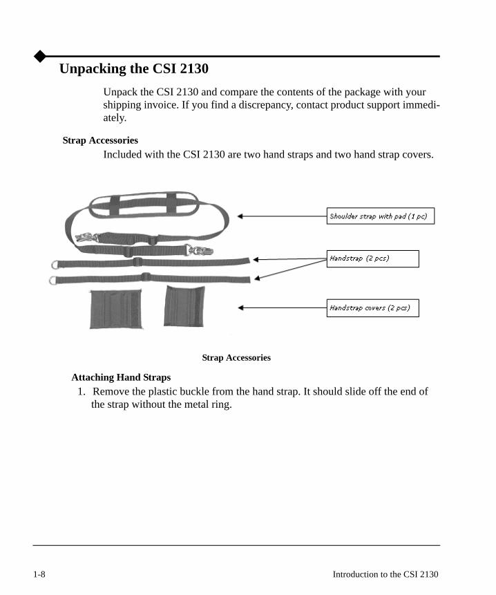
Unpacking the CSI 2130Unpack the CSI 2130 and compare the contents of the package with your shipping invoice. If you find a discrepancy, contact product support immedi-ately.
Strap AccessoriesIncluded with the CSI 2130 are two hand straps and two hand strap covers.
Strap Accessories
Attaching Hand Straps1. Remove the plastic buckle from the hand strap. It should slide off the end of
the strap without the metal ring.
1-8 Introduction to the CSI 2130

2. Starting with either the right side or left side of the analyzer, slide the strap through the plastic housing as pictured below. The strap should slide completely through the metal ring at the top.
NoteIf you are right-handed, you may want to start on the right side of the analyzer and place the metal D-ring of the hand strap in the housing near the bottom of the analyzer. If you are left-handed, you may want to do the same process, but on the left side of the analyzer.
Slide the strap through the plastic housing (2)
3. Curl the strap back up and thread it through the slot in the middle of the housing. Push the strap through until it comes out of the top of the housing. Push the plain end up and through the housing.
1-9Unpacking the CSI 2130
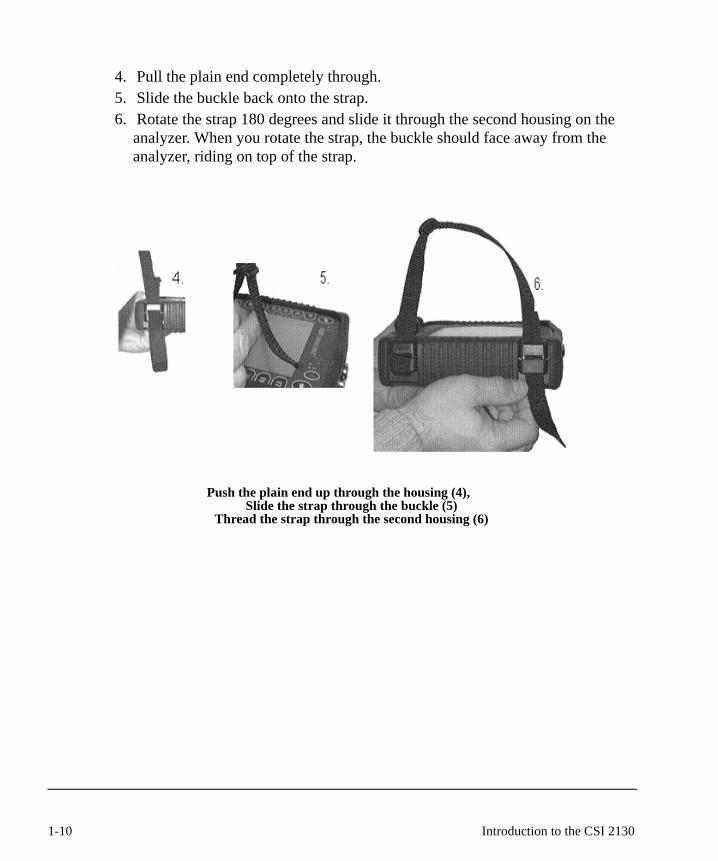
4. Pull the plain end completely through.5. Slide the buckle back onto the strap.6. Rotate the strap 180 degrees and slide it through the second housing on the
analyzer. When you rotate the strap, the buckle should face away from the analyzer, riding on top of the strap.
Push the plain end up through the housing (4), Slide the strap through the buckle (5)
Thread the strap through the second housing (6)
1-10 Introduction to the CSI 2130
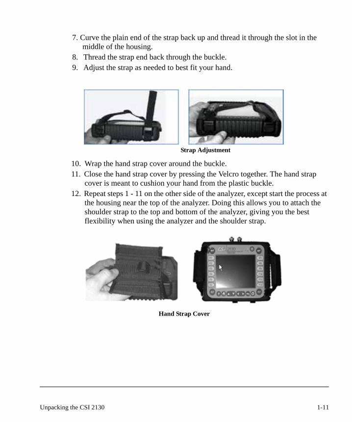
7. Curve the plain end of the strap back up and thread it through the slot in the middle of the housing.
8. Thread the strap end back through the buckle.9. Adjust the strap as needed to best fit your hand.
Strap Adjustment
10. Wrap the hand strap cover around the buckle.11. Close the hand strap cover by pressing the Velcro together. The hand strap
cover is meant to cushion your hand from the plastic buckle.12. Repeat steps 1 - 11 on the other side of the analyzer, except start the process at
the housing near the top of the analyzer. Doing this allows you to attach the shoulder strap to the top and bottom of the analyzer, giving you the best flexibility when using the analyzer and the shoulder strap.
Hand Strap Cover
1-11Unpacking the CSI 2130

Panels In addition to the battery compartment there are several panels on the CSI 2130.
Panels
Top PanelThe top of the analyzer has three types of ports or connectors:
• 25-Pin multi-function connector• ACC (Accelerometer) connector• V/Tach (Volts/Tachometer) connector
Top Panel
1-12 Introduction to the CSI 2130
25-Pin Connector• Provides connection for serial data communications between the CSI
2130 and the host computer (prior to AMS Suite: Machinery Health Manager v5.0).
• Provides input for accelerometers and other sensors and accessories.• Do not connect non-Emerson supplied cables to the analyzer’s 25-pin
connector.
Warning!Do not connect non-Emerson supplied cables to the analyzer’s 25-pin connector. To do so seriously risks damaging the analyzer since it contains many other signals and voltages in addition to what is normally found on RS232 connectors.
Warning!The 25-pin connector is not for connecting to a printer.
Accelerometer ConnectorProvides for connection of an accelerometer.
Tach ConnectorProvides for connection for a once-per-revolution pulse signal (greater than one volt), or a non-powered volts input signal.
Bottom PanelThe Bottom panel has two bays in it; one containing three ports and another containing one Ethernet Port and one Secure Digital (SD) memory card slot.
Each bay has a rubber plug covering it. To access the bays, pull open the gas-kets.
Charger InputInput from the battery charger/power supply. Plug the battery charger in here and connect to a standard 110 V or 230 V outlet to recharge the analyzer’s internal battery.
1-13Unpacking the CSI 2130
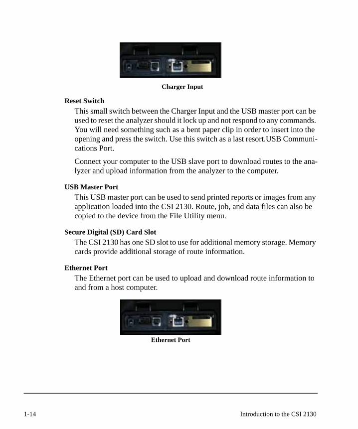
Charger Input
Reset SwitchThis small switch between the Charger Input and the USB master port can be used to reset the analyzer should it lock up and not respond to any commands. You will need something such as a bent paper clip in order to insert into the opening and press the switch. Use this switch as a last resort.USB Communi-cations Port.
Connect your computer to the USB slave port to download routes to the ana-lyzer and upload information from the analyzer to the computer.
USB Master PortThis USB master port can be used to send printed reports or images from any application loaded into the CSI 2130. Route, job, and data files can also be copied to the device from the File Utility menu.
Secure Digital (SD) Card SlotThe CSI 2130 has one SD slot to use for additional memory storage. Memory cards provide additional storage of route information.
Ethernet Port The Ethernet port can be used to upload and download route information to and from a host computer.
Ethernet Port
1-14 Introduction to the CSI 2130

Install or remove cards only when the CSI 2130 is turned off.
Memory Cards
1-15Unpacking the CSI 2130

Front Panel: Buttons, Indicators, and Keys
The following are brief descriptions of the functions located on the front panel of the CSI 2130.
On/Off Button — Controls the power on/off. Press once to turn on; press again to turn off.
Enter Buttons — Press to save your selections or initiate data collection. Use this button after you have made changes, such as setting up a job, that you want to save to the analyzers abbreviation “ALT” appears at the top of the screen and the text boxes on the left and right sides of the screen are high-lighted in yellow.) memory. Dual-enter buttons are provided for right or left hand operation.
F1 – F12 Function keys — These keys are context sensitive, which means they will change with the screens selected.
(Alternate) Button — Press this button to switch to an alternate screen giving you more choices within a menu (Not all screens have an alternate page). For those screens that do, the abbreviation “ALT” appears at the top of the screen and the text boxes on the left and right sides of the screen are high-lighted in yellow.)
Front Panel
1-16 Introduction to the CSI 2130
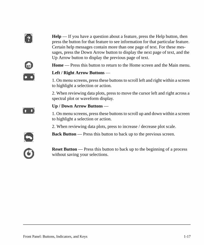
Help — If you have a question about a feature, press the Help button, then press the button for that feature to see information for that particular feature. Certain help messages contain more than one page of text. For these mes-sages, press the Down Arrow button to display the next page of text, and the Up Arrow button to display the previous page of text.
Home — Press this button to return to the Home screen and the Main menu.
Left / Right Arrow Buttons —
1. On menu screens, press these buttons to scroll left and right within a screen to highlight a selection or action.
2. When reviewing data plots, press to move the cursor left and right across a spectral plot or waveform display.
Up / Down Arrow Buttons —
1. On menu screens, press these buttons to scroll up and down within a screen to highlight a selection or action.
2. When reviewing data plots, press to increase / decrease plot scale.
Back Button — Press this button to back up to the previous screen.
Reset Button — Press this button to back up to the beginning of a process without saving your selections.
1-17Front Panel: Buttons, Indicators, and Keys
Battery Use and CareA rechargeable battery pack powers the CSI 2130. Before using the analyzer, verify that the battery has enough charge to operate properly. The battery needs to be recharged if the analyzer will not power up, or if the analyzer dis-plays a low battery warning and turns itself off.
The Battery Capacity function gives an approximate indication (in percent) of the battery’s condition. At the Home screen, you will see a bar graph showing the charge level of the battery. The bar graph is also displayed from the Route application, at the More point Info screen.
NoteTo get to the Home screen from any other screen, press the Home button on the front of the analyzer.
1-18 Introduction to the CSI 2130
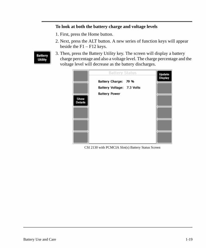
To look at both the battery charge and voltage levels
1. First, press the Home button. 2. Next, press the ALT button. A new series of function keys will appear
beside the F1 – F12 keys.3. Then, press the Battery Utility key. The screen will display a battery
charge percentage and also a voltage level. The charge percentage and the voltage level will decrease as the battery discharges.
CSI 2130 with PCMCIA Slot(s) Battery Status Screen
1-19Battery Use and Care
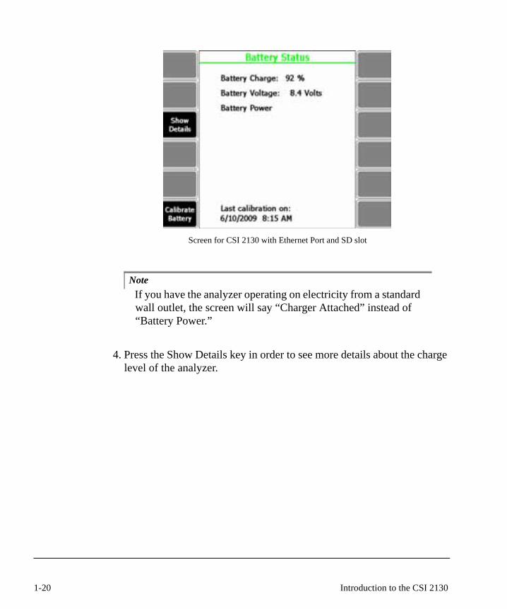
Screen for CSI 2130 with Ethernet Port and SD slot
NoteIf you have the analyzer operating on electricity from a standard wall outlet, the screen will say “Charger Attached” instead of “Battery Power.”
4. Press the Show Details key in order to see more details about the charge level of the analyzer.
1-20 Introduction to the CSI 2130

CSI 2130 with PCMCIA Slot(s) Memory Information Screen
CSI 2130 with Ethernet port and SD slot
1-21Battery Use and Care
NoteIt is not necessary to press the Show Details key, as most of the information is used for diagnostic purposes.
5. Press the Update Display key (CSI 2130 with PCMCIA slot[s] only) to update the display.
NoteThis information is automatically updated in the CSI 2130 with Ethernet port and SD slot.
6. Press the Back button to return to the previous screen and function keys.
NoteIf the battery is extremely low, the 2130 will come on, display a low battery message, then turn off.
NoteThe Battery Status information presents approximate values and should be used only as a guideline in determining the amount of remaining battery charge.
1-22 Introduction to the CSI 2130
Battery Discharge (CSI 2130 with Ethernet port and SD slot only)
When the external power supply/charger is plugged into the CSI 2130 the bat-tery charge circuit has the ability to control a battery discharge. Discharging the pack allows the gas gauge circuitry to be calibrated. During the discharge cycle the charge circuit monitors the voltage of the battery pack and termi-nates the discharge once the pack is discharged. Once the pack is discharged, the charging circuit automatically stops the discharge and starts charging in fast mode.
The gas gauge circuitry exists to provide information about the status of the analyzer’s battery pack. The primary purpose is to report the amount of charge remaining in the battery pack. Additional information includes how many times the pack has been charged since it was calibrated, how much charge was available after the last “Last Measured Discharge” (a calibration cycle), and other status information. The Gas Gauge IC also has an “EMPTY” output pin that is wired to the analyzer.
Discharging the battery is not a trivial task. The amount of time require to dis-charge and recharge the analyzer will vary between 16-30 hours depending on the initial charge level of the battery, the condition of the battery, and the hardware revision of the CSI 2130. Therefore, initiate the discharge when you have enough time to do so, such as over night or over the weekend.
1-23Battery Use and Care

To discharge the battery:
1. First make sure the external power supply/charger is plugged into the CSI 2130.
2. Next, from the Battery Status screen, press the Calibrate Battery key.3. Then, press the Enter button.
1-24 Introduction to the CSI 2130

NoteTo abort the battery calibration operation, press the Back button. Press the Enter button to continue with the battery calibration operation.
4. Wait! This is going to take awhile.5. The Abort Keys are available and will stop the discharge process.
1
The battery calibration operation consists of four steps:
Step 1 (First Discharge): This step will completely discharge the battery to remove the unknown (un-calibrated) charge.
Step 2 (First Charge): This step will fully charge the battery to prepare it for calibration.
Step 3 (Second Discharge): This step will completely discharge the battery to measure the capacity.
Step 4 (Second Charge): This step will fully charge the battery to prepare it for normal use.
1-25Battery Use and Care

If the external power supply/charger is not plugged into the CSI 2130 when the battery calibration operation is initiated an error message will appear. Either plug the external power supply/charger into the CSI 2130, then press the Enter button to continue with the battery calibration operation or press the Reset button to abort the battery calibration operation.
2
LED for Charging
A small red light on the front panel of the 2130 helps you when charging the battery. The list below tells you what the flashing or non-flashing light means.
On or Steady light – Fast charge is in process. Charging the battery pack can take several hours if the battery is completely discharged.
Flashes “50/50” – After the fast charge is complete, the LED will flash 50 percent on, 50 percent off. Fast charge is complete and the charger is in trickle charge mode. You can leave the 2130 on the charger for another 3 hours to “top it off.” This is required to fully charge the battery.
NoteIf the charger is disconnected while in trickle charge mode, and then plugged back in, the charger will go into fast charge mode for a short time before it goes back to trickle charge.
1-26 Introduction to the CSI 2130
Flashes – Mostly Off/Quick On – Action is pending. The 2130 is getting ready to allow charging of the battery pack. Battery back may be too cold or too hot for charging. Battery back should be charged at normal room temper-ature. Don’t charge in a very hot or very cold temperature environment.
If you leave the 2130 unused for two weeks, it should still have most of its charge; but it is recommended that you charge the 2130 the night before you intend to use it.
NoteThe 2130 can be operated from a standard wall electrical outlet, using the battery charger/power supply. Hook up the analyzer as described below, turn the analyzer on, and operate it.
Recharging the Battery Pack
The battery charger/power supply is used to charge the analyzer’s battery pack. To recharge the battery pack:
1. Make sure the CSI 2130 is turned off.2. Insert the power supply’s output plug into the battery charger jack located
on the bottom panel of the analyzer.3. Plug the power supply’s AC cord into a standard AC outlet.
The battery charger will recharge a fully discharged battery pack in about 3 hours. After the battery has been almost fully charged, the battery charger switches to a trickle charge mode to finish charging.
NoteThe power supply can operate from an AC outlet ranging from 100 VAC to 250 VAC, 50 to 60 Hz.
NoteIt is normal for the back of the analyzer’s case to become warm to the touch towards the end of charging.
1-27Battery Use and Care

Changing the Battery
To change the CSI 2130 analyzer’s battery pack:
1. Make sure the analyzer is off, the battery charger power supply is disconnected from the analyzer, and that the hand straps are removed.
2. Remove the rubber boot from the analyzer.3. On the back of the analyzer, remove the six screws on the back panel.
Then remove the panel.4. Carefully remove the battery pack from the battery compartment.
Analyzer with back cover removed
5. Unplug the battery from the connector to the analyzer.
Unplugging the battery from the connector.
1-28 Introduction to the CSI 2130

6. Connect the new battery pack and insert it into the analyzer case.7. Tuck the battery pack foam inserts into the case on the sides of the battery
pack. Make sure the foam inserts do not interfere with the installation of the bottom panel.
8. Replace the bottom panel and screws.9. Replace the rubber boot and any hand straps removed.
1-29Battery Use and Care

1-30 Introduction to the CSI 2130

Chapter 2
Shell Program Overview
The CSI 2130 Shell
The CSI 2130 shell program has options that affect all other programs in the analyzer.
These settings can be changed once or as often as you like.
Shell programs are listed on the left side of the home screen
2-1
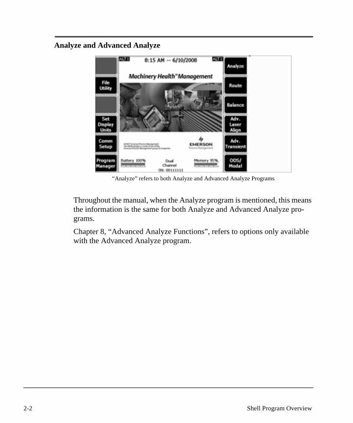
Analyze and Advanced Analyze
“Analyze” refers to both Analyze and Advanced Analyze Programs
Throughout the manual, when the Analyze program is mentioned, this means the information is the same for both Analyze and Advanced Analyze pro-grams.
Chapter 8, “Advanced Analyze Functions”, refers to options only available with the Advanced Analyze program.
2-2 Shell Program Overview

Basic SetupThis section describes one-time setup instructions for
• File Utility• Set Display Units• Comm Setup• Program Manager
File Utility
Use File Utility to select and delete files.
1 . .From the Home screen, press File Utility to open the File Utility screen with a list of files.
File Utility screen
NoteSet Source Card is available if a memory card is installed.
2-3Basic Setup

2. . .Press File Up and File Down to highlight an individual file.3. . .Press Page Up and Page Down to scroll through many files.4. . .Press Select File to mark a file to delete. Mark all the files you want to
delete.
File Utility screen with a file selected and the Delete function key active.
5. . .Press Delete. A warning message appears.
File Utility Warning dialog box.
6. . .To delete the selected file(s), press Enter. To escape and save these files, press Back.
2-4 Shell Program Overview

To Delete All the Files at OnceIf you want to select all of your files at the same time, press ALT. Press Select All Files. Press ALT, and then press Delete to clear all files.
File Utility Alt screen with Select All Files selected.
Memory CardsDepending on the version, the CSI 2130 can handle either one or two memory cards to expand memory. You may want to store different routes on different individual cards.
NoteThe CSI 2130 with PCMCIA slots will have either 1 or 2 PCMCIA slots depending on its version. Ethernet Cards and Compact Flash Memory Cards work in both slots. The CSI 2130 with an Ethernet port and SD slot has 1 SD slot.
Also, a USB drive can be plugged into the USB port on the CSI 2130 with Ethernet port and SD slot for transferring route and job files.
2-5Basic Setup
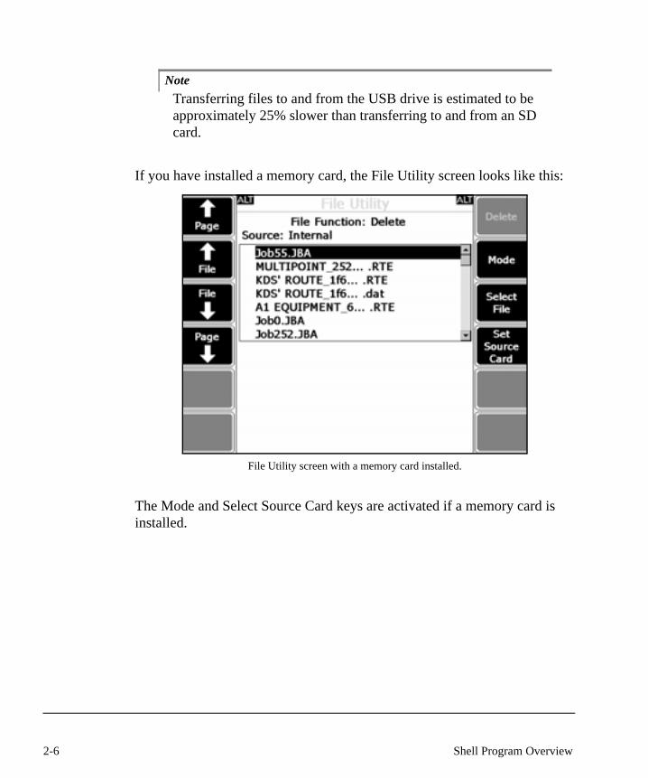
NoteTransferring files to and from the USB drive is estimated to be approximately 25% slower than transferring to and from an SD card.
If you have installed a memory card, the File Utility screen looks like this:
File Utility screen with a memory card installed.
The Mode and Select Source Card keys are activated if a memory card is installed.
2-6 Shell Program Overview

Mode: Toggle though the choices Delete, Move, and Copy. For Move and Copy options, the bottom half of the screen shows the destination of the copy or move.
File Utility screen with Copy selected.
Set Source Card: Switch Source and Destination directories. The Source directory may be the Internal directory of files or the Card directory.
NoteThe bottom section of your display screen displays the destina-tion directory and the upper section displays the source direc-tory.
Page Up and Page Down: Scroll through the Destination directory.
NoteYou can only copy, move, remove, or delete files from the Source directory to the Destination directory.
2-7Basic Setup

Select All Files: Selects all the files in the Source directory (folder). This is an ALT screen function.
Memory Card(s)Depending on the version of the CSI 2130, you can have one or two memory cards installed at the same time.
File Utility screen with two cards installed in the analyzer.
Set Source Card: Selects the Source directory (folder) for copying or moving files to the Destination directory. The Source directory can be Internal, Card, Card2 (if you have the two-slot PCMCIA version), or USB drive (if you have a USB drive plugged into the USB port on a CSI 2130 with an Ethernet port and SD slot). The Source and the Destination directories cannot be the same.
Set Dest(ination) Card: Selects the Destination directory (folder) for copying or moving files from the Source directory. The Destination directory can be Internal, Card, Card2 (if you have the two-slot PCMCIA version), or USB drive (if you have a USB drive plugged into the USB port on a CSI 2130 with an Ethernet port and SD slot). The Source and the Destination directories, however, cannot be the same Directory.
2-8 Shell Program Overview

The Source directory appears in the upper window on the screen and the Des-tination directory appears in the lower window of the screen.
2-9Basic Setup

Set Display Units
Display Units define how the CSI 2130 collects and displays data.
Set Display Units screen
Set Display Units for:
• Acceleration• Velocity• Displacement• Non-Standard• English or Metric measurements• Decibel References• Plot Vertical (Y) Axis Type• Frequency X Axis Type• Frequency units measured in Hertz (Hz) or Cycles per Minute (CPM)
2-10 Shell Program Overview

Set Accel(eration): Choose RMS, Peak, Peak to Peak, Average, or DB. RMS (root mean square) is the default.
Set Display Units, Set Accel(eration)
Set Veloc(ity): Choose RMS, Peak, Peak to Peak, Average, or DB. Peak is the default.
Set Displace(ment): Choose RMS, Peak, Peak to Peak, Average, DB. Peak to Peak is the default.
xSet Non Standard: Choose RMS, Peak, Peak to Peak, Average, or DB. RMS is the default.
Set Units: Press to toggle measurement display in English, Metric and SI units.
2-11Basic Setup
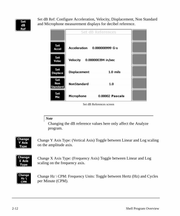
Set dB Ref: Configure Acceleration, Velocity, Displacement, Non Standard and Microphone measurement displays for decibel reference.
Set dB References screen
NoteChanging the dB reference values here only affect the Analyze program.
Change Y Axis Type: (Vertical Axis) Toggle between Linear and Log scaling on the amplitude axis.
Change X Axis Type: (Frequency Axis) Toggle between Linear and Log scaling on the frequency axis.
Change Hz \ CPM: Frequency Units: Toggle between Hertz (Hz) and Cycles per Minute (CPM).
2-12 Shell Program Overview

Communications Setup
Communications setup lets you configure communications between the CSI 2130 and AMS Suite: Machinery Health Manager on your computer or net-work.
Comm Setup screen
Set Connect(ion) Port – Press to select an Ethernet Card, USB, or Serial Port Connection. Highlight the option you are using and press Enter.
Connection Port dialog box
NoteThe fastest way of making connection is Ethernet. The second fastest is USB. The slowest is Serial Port.
2-13Basic Setup

USB Port ConnectionTo begin using a USB Port connection, press Change Device ID to set the name of your 2130. No further configuration is needed from this screen if you are using a USB Port.
Change Device Name: Enter a unique name for your CSI 2130.
Device Name Edit dialog box
NoteFor additional text tools, press the ALT button and a different set of characters and text tools appears. Use the ALT button to toggle between these two sets.
NoteThe device name appears on the screen in Data Transfer to iden-tify the particular CSI 2130 analyzer.
2-14 Shell Program Overview
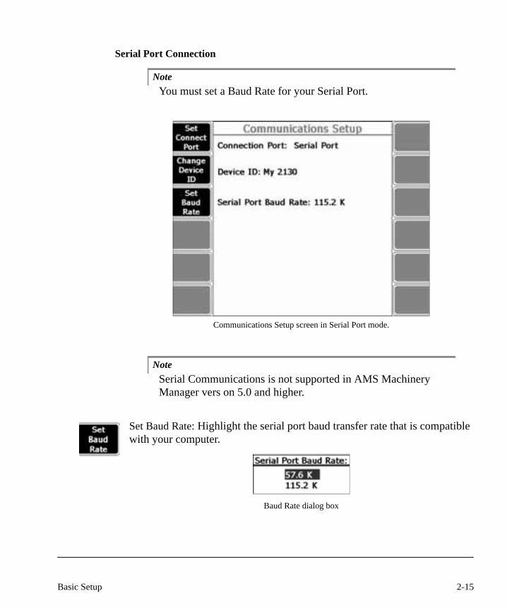
Serial Port Connection
NoteYou must set a Baud Rate for your Serial Port.
Communications Setup screen in Serial Port mode.
NoteSerial Communications is not supported in AMS Machinery Manager vers on 5.0 and higher.
Set Baud Rate: Highlight the serial port baud transfer rate that is compatible with your computer.
Baud Rate dialog box
2-15Basic Setup
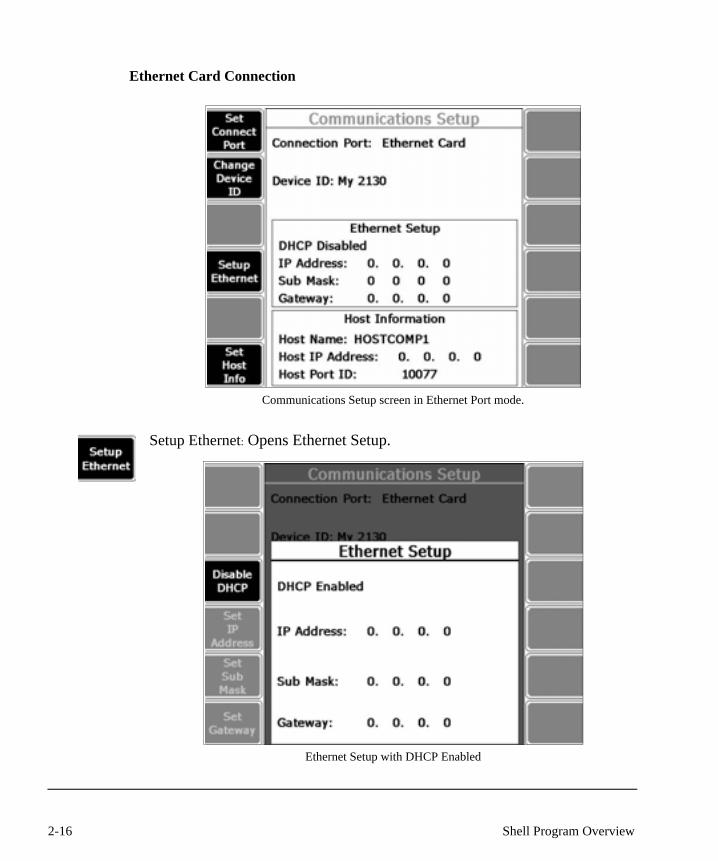
Ethernet Card Connection
Communications Setup screen in Ethernet Port mode.
Setup Ethernet: Opens Ethernet Setup.
Ethernet Setup with DHCP Enabled
2-16 Shell Program Overview
NoteYour Ethernet settings depend on your local networks. You will need information and assistance from your information technol-ogies department.
Dynamic Host Configuration Protocol (DHCP)Dynamic Host Configuration Protocol, or DHCP, is an Internet protocol that automates the configuration of computers that use TCP/IP. DHCP automati-cally assigns IP addresses to deliver TCP/IP stack configuration parameters, such as the subnet mask and default router. DHCP also provides other config-uration information.
If you are using an Ethernet Card with your CSI 2130, you can use either DHCP or a static IP address to communicate. You need to check with your information technologies department to see if DHCP is supported.
NoteIf your workplace does not support DHCP, then your informa-tion technologies department needs to provide you a valid IP Address, SubMask, and Gateway.
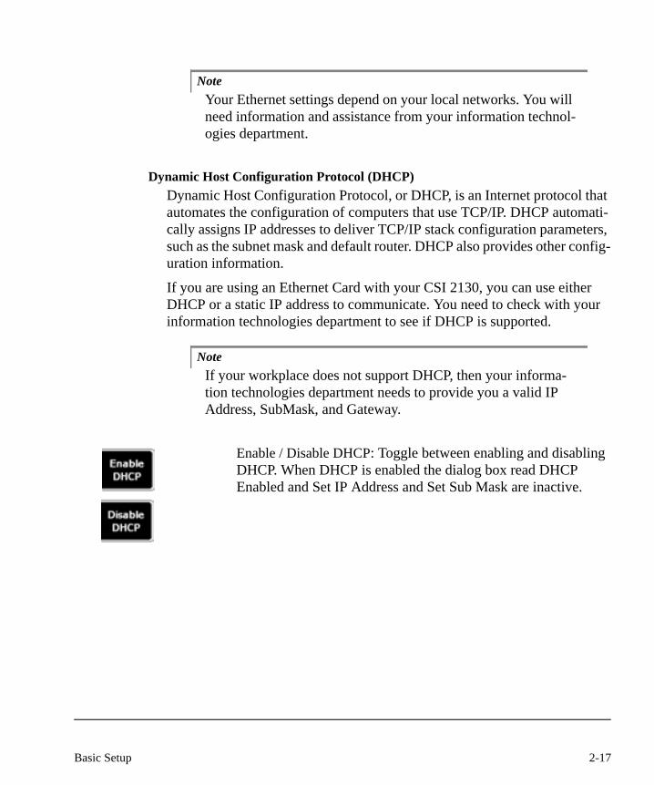
Enable / Disable DHCP: Toggle between enabling and disabling DHCP. When DHCP is enabled the dialog box read DHCP Enabled and Set IP Address and Set Sub Mask are inactive.
2-17Basic Setup
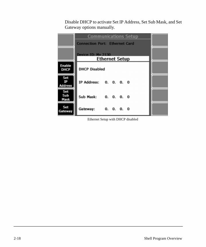
Disable DHCP to activate Set IP Address, Set Sub Mask, and Set Gateway options manually.
Ethernet Setup with DHCP disabled
2-18 Shell Program Overview

Set IP Address, Set SubMask, and Set Gateway: Use the number keys to enter a number for each position. Press the Right Arrow to move to the next box. Do this for each position number and press Enter to return to Communications Setup.
Ethernet Setup screen with IP Address selected.
2-19Basic Setup
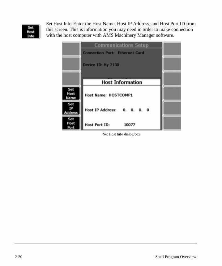
Set Host Info: Enter the Host Name, Host IP Address, and Host Port ID from this screen. This is information you may need in order to make connection with the host computer with AMS Machinery Manager software.
Set Host Info dialog box
2-20 Shell Program Overview
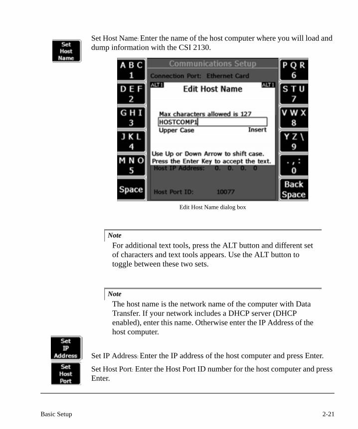
Set Host Name: Enter the name of the host computer where you will load and dump information with the CSI 2130.
Edit Host Name dialog box
NoteFor additional text tools, press the ALT button and different set of characters and text tools appears. Use the ALT button to toggle between these two sets.
NoteThe host name is the network name of the computer with Data Transfer. If your network includes a DHCP server (DHCP enabled), enter this name. Otherwise enter the IP Address of the host computer.
Set IP Address: Enter the IP address of the host computer and press Enter.
Set Host Port: Enter the Host Port ID number for the host computer and press Enter.
2-21Basic Setup
NoteDo not change the Host Port ID number unless you are instructed by CSI customer support.
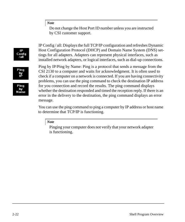
IP Config / all: Displays the full TCP/IP configuration and refreshes Dynamic Host Configuration Protocol (DHCP) and Domain Name System (DNS) set-tings for all adapters. Adapters can represent physical interfaces, such as installed network adapters, or logical interfaces, such as dial-up connections.
Ping by IP/Ping by Name: Ping is a protocol that sends a message from the CSI 2130 to a computer and waits for acknowledgment. It is often used to check if a computer on a network is connected. If you are having connectivity problems, you can use the ping command to check the destination IP address for you connection and record the results. The ping command displays whether the destination responded and timed the reception reply. If there is an error in the delivery to the destination, the ping command displays an error message.
You can use the ping command to ping a computer by IP address or host name to determine that TCP/IP is functioning.
NotePinging your computer does not verify that your network adapter is functioning.
2-22 Shell Program Overview
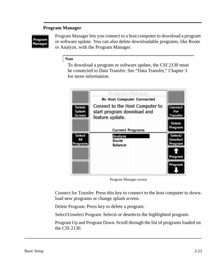
Program Manager
Program Manager lets you connect to a host computer to download a program or software update. You can also delete downloadable programs, like Route or Analyze, with the Program Manager.
NoteTo download a program or software update, the CSI 2130 must be connected to Data Transfer. See “Data Transfer,” Chapter 3 for more information.
Program Manager screen
Connect for Transfer: Press this key to connect to the host computer to down-load new programs or change splash screen.
Delete Program: Press key to delete a program.
Select/Unselect Program: Selects or deselects the highlighted program.
Program Up and Program Down: Scroll through the list of programs loaded on the CSI 2130.
2-23Basic Setup
Select All Programs: Press to select all of the current programs listed.
Delete Splash Screen: Press Delete Splash Screen to clear the custom graphic currently displayed on your home screen. The Delete Splash Screen key is only visible if a custom splash screen has been installed. The default splash screen, pictured on page 2-33, cannot be deleted.
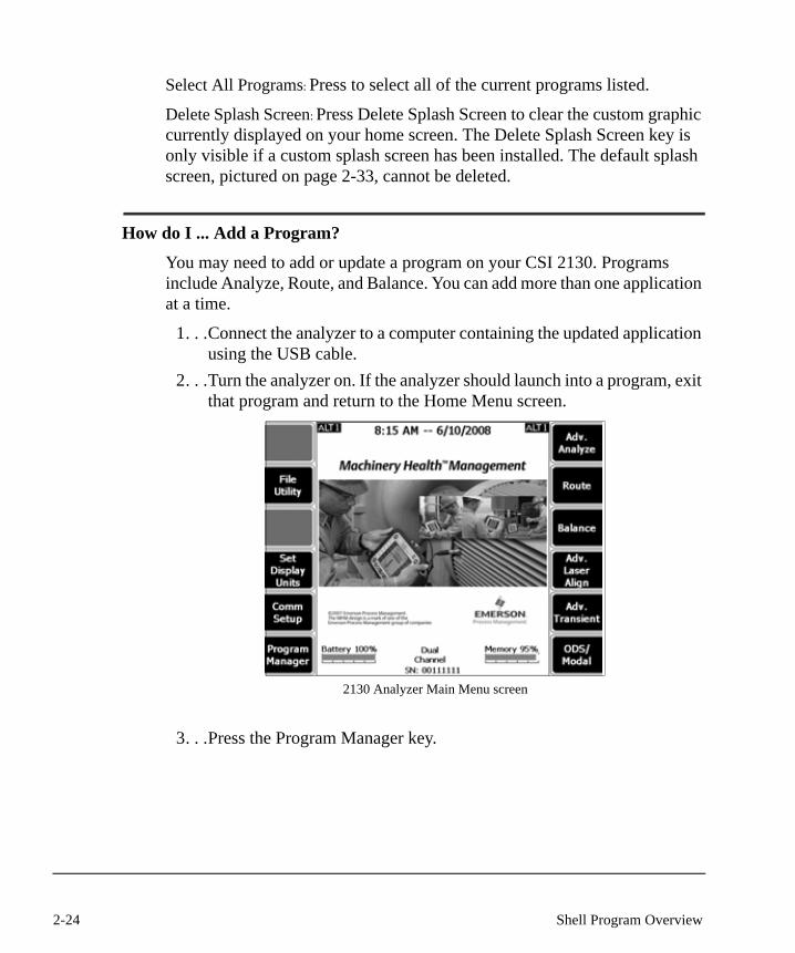
How do I ... Add a Program?
You may need to add or update a program on your CSI 2130. Programs include Analyze, Route, and Balance. You can add more than one application at a time.
1. . .Connect the analyzer to a computer containing the updated application using the USB cable.
2. . .Turn the analyzer on. If the analyzer should launch into a program, exit that program and return to the Home Menu screen.
2130 Analyzer Main Menu screen
3. . .Press the Program Manager key.
2-24 Shell Program Overview
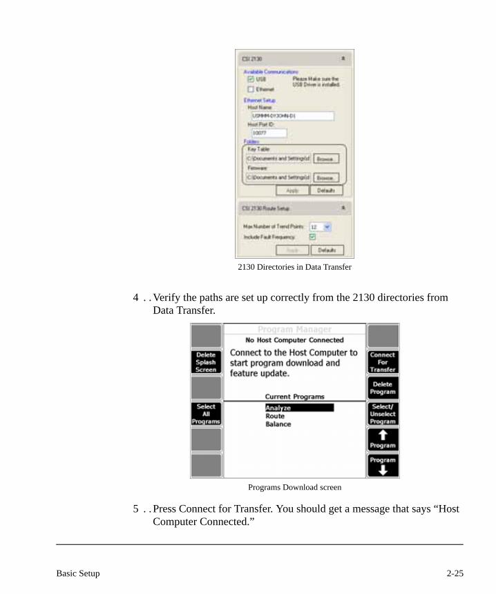
2130 Directories in Data Transfer
4 . .Verify the paths are set up correctly from the 2130 directories from Data Transfer.
Programs Download screen
5 . .Press Connect for Transfer. You should get a message that says “Host Computer Connected.”
2-25Basic Setup

Possible Base Firmware Error Messages
This message forces you to update your base firmware
If you get error message above, you must update your base firmware before continuing. The CSI 2130 will not let you use any programs until you update the base firmware.
This message alerts you that a newer version of base firmware is available.
If you get the error message above, it means the CSI 2130 has detected a newer version of base firmware on your CD, but you are not forced to update to continue downloading your programs.
2-26 Shell Program Overview

Once You’re Connected ...In the screen below, the host computer is connected to the CSI 2130 and the programs available for download are listed. This view shows you that you can update the programs you have currently loaded into your CSI 2130 (Analyze and Route), and you can add the Balance program.
The CSI 2130 is connected and the programs available for download are listed.
6 . .Press Program Up and Down to highlight the program you want to add. Next, press Select/Unselect Program to select one program, or press Select All Programs if you want to select all the programs available to download.
2-27Basic Setup

The screen below shows that the “Update current programs” and Balance have been selected for download.
The program update and Balance are selected for download.
7. . .Press Start Download. When the program is downloaded, the screen below appears:
Programs update screen
Press Enter or Reset to return to the home screen.
2-28 Shell Program Overview
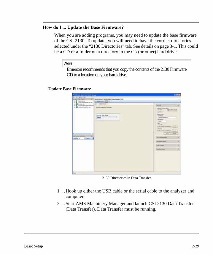
How do I ... Update the Base Firmware?
When you are adding programs, you may need to update the base firmware of the CSI 2130. To update, you will need to have the correct directories selected under the “2130 Directories” tab. See details on page 3-1. This could be a CD or a folder on a directory in the C:\ (or other) hard drive.
NoteEmerson recommends that you copy the contents of the 2130 Firmware CD to a location on your hard drive.
Update Base Firmware
2130 Directories in Data Transfer
1 . .Hook up either the USB cable or the serial cable to the analyzer and computer.
2 . .Start AMS Machinery Manager and launch CSI 2130 Data Transfer (Data Transfer). Data Transfer must be running.
2-29Basic Setup

3. . .With the CSI 2130 off, press the lower left ALT and the Power buttons. Hold down until the analyzer turns on. The CSI Special Functions Menu appears.
CSI 2130 Analyzer Special Functions screen
From here you can press the F1 function key to learn about Bootload, F2 to update the firmware using the USB connection or F3 to update firmware using the serial connection.
2-30 Shell Program Overview

NoteAMS Machinery Manager v.5.0 and above does not support serial communications for the CSI 2130. Firmware must be loaded using USB.
3 . .Press F2 or F3. The analyzer will attempt to make connection to the computer. Once the connection is made the firmware begins updating.
4 . .When done the analyzer shuts itself off. You can now turn it back on and begin using it.
NoteUpdating the firmware does not update the applications. Pro-grams must be updated separately. See “How do I ... Add a Pro-gram?” on page 2-24 for more information.
NoteIf the analyzer gets stuck trying to make connection, press the Power button to turn the analyzer off. You can then try again.
2-31Basic Setup
How do I .. Delete a Program?
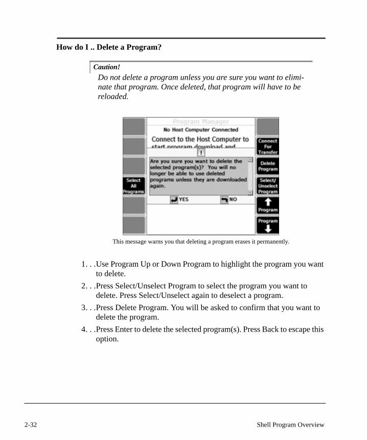
Caution!Do not delete a program unless you are sure you want to elimi-nate that program. Once deleted, that program will have to be reloaded.
This message warns you that deleting a program erases it permanently.
1. . .Use Program Up or Down Program to highlight the program you want to delete.
2. . .Press Select/Unselect Program to select the program you want to delete. Press Select/Unselect again to deselect a program.
3. . .Press Delete Program. You will be asked to confirm that you want to delete the program.
4. . .Press Enter to delete the selected program(s). Press Back to escape this option.
2-32 Shell Program Overview

How do I... Load a New Splash Screen?
Change the default graphic on the 2130 home screen to reflect your company’s logo.
You can change the graphic on your home screen to your company’s logo. First, find the graphic you want to use.
NoteThe graphic must be 430w x 380h pixels to display properly on your 2130. If your splash.bmp image is larger than the required format, only a portion of the picture will show on the screen. If the image is smaller than the required format, it will be centered on the screen. It is best to limit the color palette for the image to the 256 color (8-bit) palette.
You need to save the graphic as a bitmap, and rename the graphic “splash.bmp” when you save it. Otherwise, the 2130 will not recognize the file for transfer. Save this graphic to the firmware folder on your computer.
Open CSI 2130 Data Transfer from the AMS Machinery Manager setup/com-munications tab. Right click on the CSI 2130 device and select configure.
2-33Basic Setup

From the Folders view, verify the custom splash.bmp file is located in the specified directory for the firmware and select apply.
Turn on your CSI 2130 and press Program Manager from the home screen.
Press Delete Splash Screen to clear the custom graphic currently displayed on your home screen. The Delete Splash Screen key is only visible if a custom splash screen has been installed. The default splash screen, pictured on page 2-33, cannot be deleted.
NoteNo warning is given before the custom splash screen is deleted.
Then press Connect for Transfer. Once the 2130 connects to the computer and the proper location, it will tell you which files are available to download.
Press Load New Splash Screen to download a new graphic.
2-34 Shell Program Overview

Press Load New Splash Screen to load your new graphic. The CSI 2130 reads “Loading Splash File.” This key does not display if you have not connected to the computer and created a custom splash.bmp file.
This message appears when your custom splash.bmp graphic is loading.
The “Loading Splash File” message disappears and you return to the Pro-grams Download screen. Press Home to view the new graphic on your home screen.
Your new graphic displays on the home screen.
2-35Basic Setup

ALT: Alternate Screens
ALT Screen
Press ALT on any screen with ALT icons at the top to get a second screen of options:
Home Screen (left) and Home ALT Screen (right)
This section describes these Alternate Screen features:
• Version Information• General Setup• Setting Time• Memory Utility• Battery Utility• Viewing Error Logs• Connect to Virtual Printer
2-36 Shell Program Overview
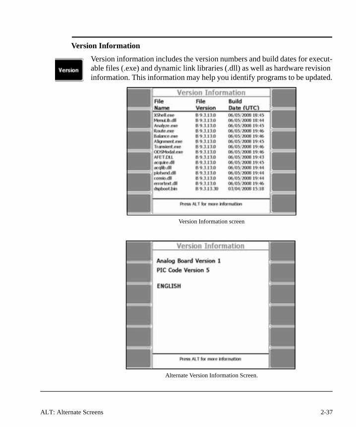
Version Information
Version information includes the version numbers and build dates for execut-able files (.exe) and dynamic link libraries (.dll) as well as hardware revision information. This information may help you identify programs to be updated.
Version Information screen
VV
Alternate Version Information Screen.
2-37ALT: Alternate Screens

General Setup
Use General Setup to control beeper, display, and power off settings.
General Analyzer Setup screen
Set Keypad Beeper: Press to toggle on and off. If the beeper is on, the CSI 2130 beeps each time you press a key.
Set Status Beeper: Press to toggle on and off. If this beeper is on, the CSI 2130 beeps for alerts and other indications.
2-38 Shell Program Overview

Set Power Off: Automatically shuts the meter off if it goes unused for a period of time. The default time is 30 minutes, but you can change this number or enter zero (0) to disable this feature.
Set Power Off Time
2-39ALT: Alternate Screens
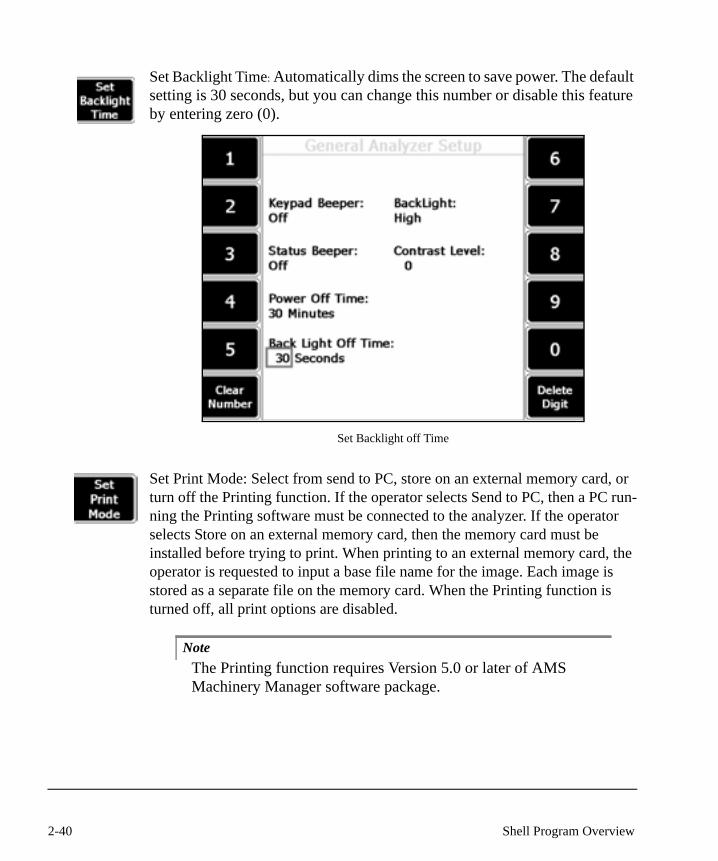
Set Backlight Time: Automatically dims the screen to save power. The default setting is 30 seconds, but you can change this number or disable this feature by entering zero (0).
Set Backlight off Time
Set Print Mode: Select from send to PC, store on an external memory card, or turn off the Printing function. If the operator selects Send to PC, then a PC run-ning the Printing software must be connected to the analyzer. If the operator selects Store on an external memory card, then the memory card must be installed before trying to print. When printing to an external memory card, the operator is requested to input a base file name for the image. Each image is stored as a separate file on the memory card. When the Printing function is turned off, all print options are disabled.
NoteThe Printing function requires Version 5.0 or later of AMS Machinery Manager software package.
2-40 Shell Program Overview
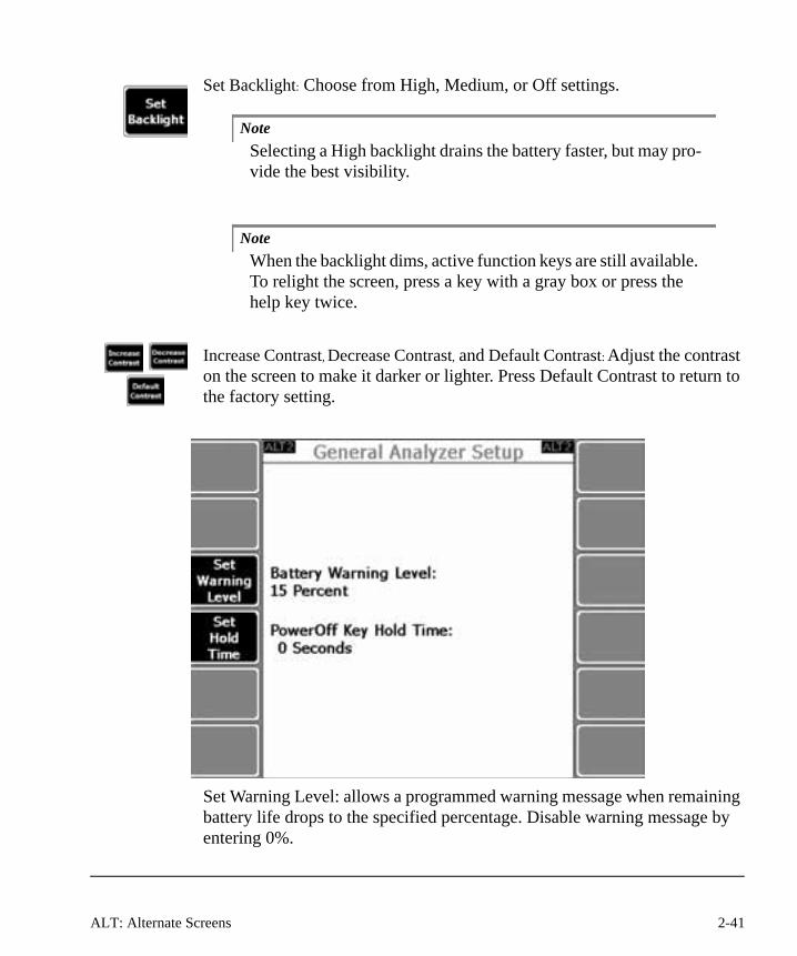
Set Backlight: Choose from High, Medium, or Off settings.
NoteSelecting a High backlight drains the battery faster, but may pro-vide the best visibility.
NoteWhen the backlight dims, active function keys are still available. To relight the screen, press a key with a gray box or press the help key twice.
Increase Contrast, Decrease Contrast, and Default Contrast: Adjust the contrast on the screen to make it darker or lighter. Press Default Contrast to return to the factory setting.
Set Warning Level: allows a programmed warning message when remaining battery life drops to the specified percentage. Disable warning message by entering 0%.
2-41ALT: Alternate Screens
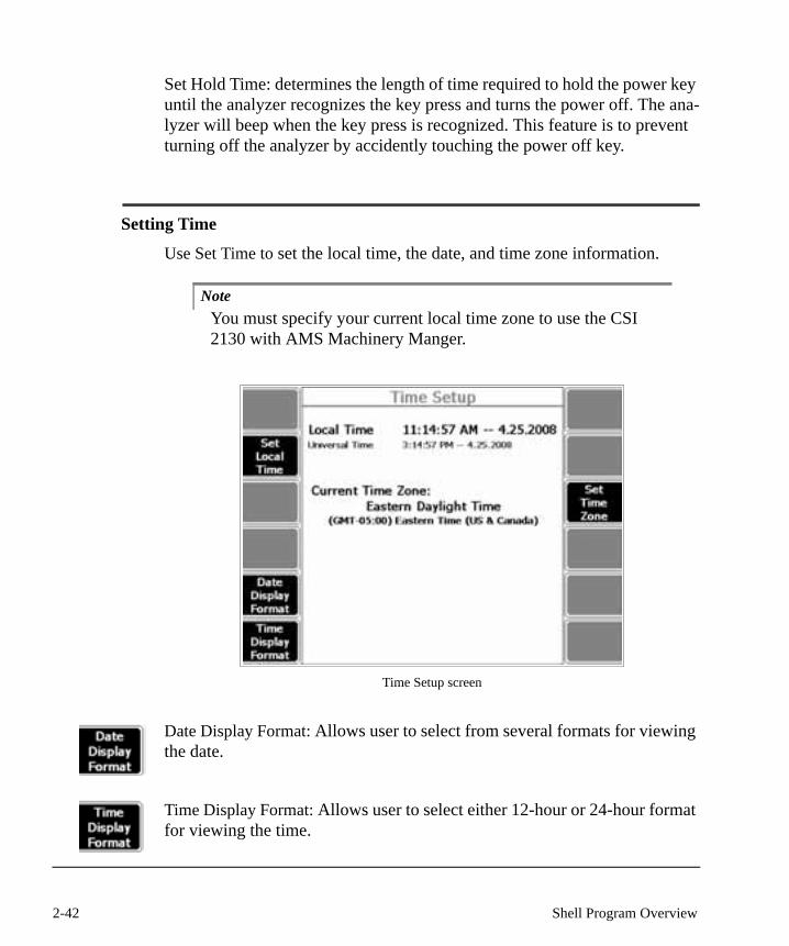
Set Hold Time: determines the length of time required to hold the power key until the analyzer recognizes the key press and turns the power off. The ana-lyzer will beep when the key press is recognized. This feature is to prevent turning off the analyzer by accidently touching the power off key.
Setting Time
Use Set Time to set the local time, the date, and time zone information.
NoteYou must specify your current local time zone to use the CSI 2130 with AMS Machinery Manger.
Time Setup screen
Date Display Format: Allows user to select from several formats for viewing the date.
Time Display Format: Allows user to select either 12-hour or 24-hour format for viewing the time.
2-42 Shell Program Overview
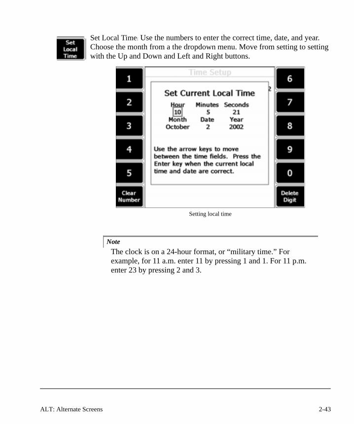
Set Local Time: Use the numbers to enter the correct time, date, and year. Choose the month from a the dropdown menu. Move from setting to setting with the Up and Down and Left and Right buttons.
Setting local time
NoteThe clock is on a 24-hour format, or “military time.” For example, for 11 a.m. enter 11 by pressing 1 and 1. For 11 p.m. enter 23 by pressing 2 and 3.
2-43ALT: Alternate Screens
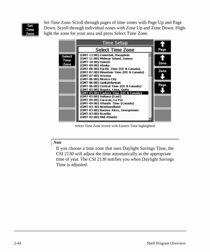
Set Time Zone: Scroll through pages of time zones with Page Up and Page Down. Scroll through individual zones with Zone Up and Zone Down. High-light the zone for your area and press Select Time Zone.
Select Time Zone screen with Eastern Time highlighted
NoteIf you choose a time zone that uses Daylight Savings Time, the CSI 2130 will adjust the time automatically at the appropriate time of year. The CSI 2130 notifies you when Daylight Savings Time is adjusted.
2-44 Shell Program Overview
Memory Utility
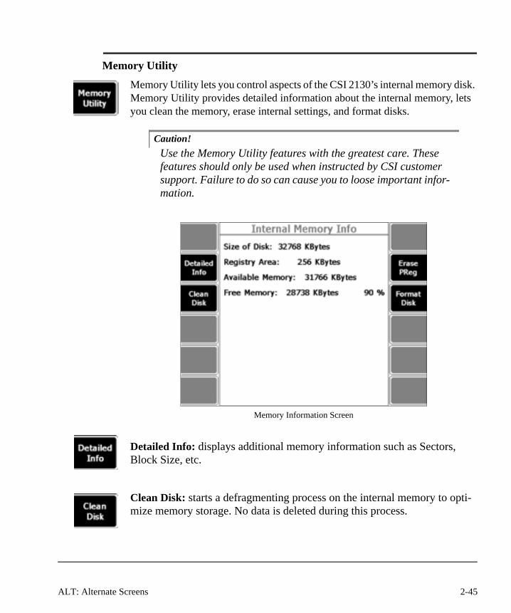
Memory Utility lets you control aspects of the CSI 2130’s internal memory disk. Memory Utility provides detailed information about the internal memory, lets you clean the memory, erase internal settings, and format disks.
Caution!Use the Memory Utility features with the greatest care. These features should only be used when instructed by CSI customer support. Failure to do so can cause you to loose important infor-mation.
Memory Information Screen
Detailed Info: displays additional memory information such as Sectors, Block Size, etc.
Clean Disk: starts a defragmenting process on the internal memory to opti-mize memory storage. No data is deleted during this process.
2-45ALT: Alternate Screens

Erase PReg: clears the internal settings of the CSI 2130 that are stored in per-manent memory. Once done, the default setting will be loaded the next time the CSI 2130 is turned on.
Caution!Do this function only if instructed to do so by CSI support per-sonnel.
Format Disk: press this key only if you need to format a disk. Formatting a disk erases all data and programs on that disk. Once done the memory is erased completely and the CSI 2130 shuts down.
NoteThe internal memory includes applications like Route, Analyze, and Balance. All routes, jobs, and data are erased if you press Format Disk. A verification message appears before you can complete formatting the disk.
See Section 1, page 26, for Battery Use and Care information.
2-46 Shell Program Overview
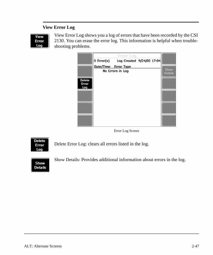
View Error Log
View Error Log shows you a log of errors that have been recorded by the CSI 2130. You can erase the error log. This information is helpful when trouble-shooting problems.
Error Log Screen
Delete Error Log: clears all errors listed in the log.
Show Details: Provides additional information about errors in the log.
2-47ALT: Alternate Screens

Connect For Printing
Connect For Printing: Establishes a connection between the analyzer and a host computer running the printing software. This allows the host computer to cap-ture and print screens from the analyzer and from the analyzer generate route reports, alignment reports, balance reports, along with individual spectrum and waveform captures and printouts. If a connection has been established between the analyzer and a host computer system, then this key will be labeled End Printing and pressing this key will remove the connection.
2-48 Shell Program Overview

Chapter 3
Data Transfer
OverviewThe Data Transfer application is used to manage the transfer of routing instructions and data to and from a portable device. The portable devices sup-ported by Data Transfer are the CSI 2130, CSI 2120, and CSI 2117 vibration analyzers and the CSI9800 and the Fluke Ti55 Infrared cameras.
NoteThe CSI 2130 analyzer must have firmware version 8.3.11 or later. The CSI 2120 analyzer must have firmware version 7.45 or later. The CSI 2117 analyzer must have firmware version 6.41 or later. Older CSI 9800 firmware versions will generate an error upon connection attempt.
The Data Transfer application supports three modes of communication between the computer and portable devices: USB, Ethernet, and serial. The CSI 2130 supports USB or Ethernet, however, the most common mode is USB. The CSI 2120 and CSI 2117 only communicate over a serial connec-tion. Another communication feature that Data Transfer offers is the ability to perform intermediate file transfer.
NoteSerial cable communications is no longer supported for the CSI 2130 analyzer.
With intermediate file transfer, the user has the option to transfer data to a file, and at a later time, that file can be transferred into an analyzer or into the data-base. This form of communication is typically used in conjunction with the Standalone Data Transfer application running on remote machines. The Standalone Data Transfer application is shipped on the firmware CD.
3-1
Remote users of the CSI 2130 analyzer have the additional option of using an Ethernet connection to the CSI Data Transfer Service running on the AMS Machinery Manager server. When the CSI 2130 analyzer connects to the CSI Data Transfer Service, all communication is driven from the analyzer user interface. Users will have to provide their AMS Machinery Manager user name and password to gain access to the database list. For further information concerning the CSI Data Transfer Service, please contact CSI customer sup-port.
Finally, the Data Transfer application is also used to update firmware and pro-grams and supports the printing functionality in the CSI 2130 analyzer. The printing functionality allows users to print a report from a route or plot directly from the CSI 2130 analyzer.
3-2 Data Transfer

Data Transfer HostAMS Machinery Manager hosts Data Transfer. Upon first access, the appli-cation will appear as shown below. Displayed in the main window will be information concerning any portable device for which communication is cur-rently enabled. The text below the portable device will display status infor-mation. The CSI 2130 displays by default and the user is required to confirm communication setup by selecting the “Apply” button before direct commu-nication is possible. To enable another device type, select the device from the “Enable Device” drop down menu.
Vibration
V
Vibration File Transfer
The bottom left side of the screen contains the notifications window. It pro-vides the state of the Data Transfer process. In addition, upon data storage to the AMS Machinery Manager database, summary information concerning the data just dumped will be displayed here. If an error occurs during pro-cessing or saving of data, it will be displayed in this area as well.
3-3Data Transfer Host

The user may clear old information out using the “Clear” drop down menu. In addition, users may turn off or on the display of notifications, summary or error information using the “Views” drop down menu. And the user may also print the notification window by right clicking on the window and choosing the print option.
The Navigator
Data Transfer uses the navigation tree as its drop point for routes, jobs and infrared measurements. In addition, routes and alignment or balance jobs may be copied from the navigation tree to a local folder or a connected CSI 2130 analyzer. The database items displayed in the navigator filter is to include only those items that may be copied. Therefore, data just saved or dumped may not display in the navigator view. Users may view saved data using the appropriate analysis or reporting application.
Device(s) Waiting For Connection List
The “Enabled Devices Tab” displays the list of devices waiting for connec-tion. It displays the icon for the device, the device name and extra informa-tion. The extra information displays if the device is still waiting for connection, or if is already connected, or if the device's configuration is in conflict with another device.
3-4 Data Transfer

CSI 2130 SetupTo configure a CSI 2130 device, right-click a device and select ‘Configure Device.’
The “Options Panel” on the right side displays and automatically shows the CSI 2130 options. From here the USB, Ethernet, Host Name, Host Port ID, Key Table and Firmware folder locations can be modified.
Configuration Options for CSI 2130
USB - Select this if communicating by USB cable. The CSI 2130 USB driver must be installed correctly for USB communications to initiate. Please see the section Installing the USB Driver for further information.
Ethernet - Check this box to configure the Ethernet setup. Most users will leave this unchecked and use the supplied USB cable for communication.
• Host Name - Use the host name of your computer or localhost.• Host Port ID – This defines the TCP/IP port that will be used to com-
municate between the CSI 2130 analyzer and the host computer. This should be left at 10077 unless otherwise directed by customer support. This setting must match the “Host Port ID” setting in the CSI 2130 ana-lyzer or communication will not initiate.
3-5CSI 2130 Setup
The CSI 2130 setup must match the "Comm Setup" selection in the CSI 2130 analyzer. The analyzer can only communicate using one method at a time. Therefore, the analyzer will need to be reconfigured in order to switch from USB to Ethernet communication. Please see the CSI 2130 manual for infor-mation concerning configuring communication setup.
Folders - These are used when updating the base firmware or loading a new key table in the CSI 2130 analyzer. These could be a CD or a folder on the local harddrive.
Key Table - Use this to select the location where the Key table folder is located. This setting is used to download a new key table to the CSI 2130 ana-lyzer. A new key table may be required to activate a new feature.
Firmware - Use this to select the location where the Firmware folder is located.
NoteIt is recommended that the contents of the CSI 2130 Firmware CD are copied to a location on the local computer’s hard drive.
Installing the USB Driver
The first time a CSI 2130 analyzer is connected to a host computer using the USB cable and ports, the CSI 2130 USB driver will need to be loaded to enable communication.
3-6 Data Transfer

NoteBefore beginning, the user must have administrator rights on the computer. Windows administrator rights are required for the driver to successfully load.
1. .Turn the CSI 2130 off and connect the analyzer and computer. Plug one end of the supplied USB cable into the analyzers USB slave port and the other end into the computer’s USB port.
2. . Press the Power button on the analyzer to turn it on. A dialog box appears on your computer screen indicating Windows has detected a new device plugged into the USB port.
3. . Next, an installation Wizard screen, similar to the one displayed below, to enable the process on installing the appropriate driver.
Found New Hardware
4. . .At this point, follow the prompts for installing the driver. When given the option, select the option to specify the driver location.
3-7CSI 2130 Setup

Install from a specific location
5. . .You will now have to find the driver location. Select the “Include this location in the search” and press the Browse button. The driver location may be found in one of three places:
a. On your AMS Machinery Manager install CD in a folder entitled “Drivers”.
b. If AMS Machinery Manager has been installed on the computer, the drivers may also be found in a folder entitled “Drivers” in the install location, usually C:\RBMsuite.
c. If running a network version of AMS Machinery Manager, the drivers may also be found on the server computer housing the RBMsuite folder.
3-8 Data Transfer
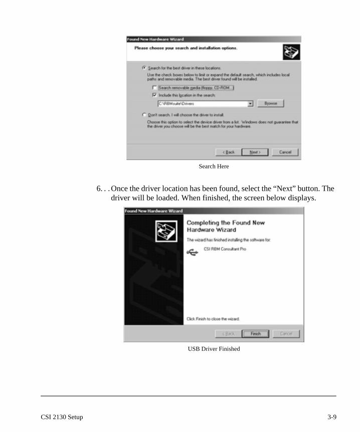
Search Here
6. . .Once the driver location has been found, select the “Next” button. The driver will be loaded. When finished, the screen below displays.
USB Driver Finished
3-9CSI 2130 Setup

NoteThe exact format and content of the dialogs presented may vary based on the Windows operating system version. However, the goal is the same and the results are the same.
Common ConfigurationThe Auto-Analyze, Data Dump, Route Load and CSI 2130 Route Setup affects the overall functionality of each for route load and dump operations.
The Data Dump SetupThe Data Dump Setup gives the user the ability to substitute dates in the route for a new date, specify what kind of data should be stored during a route dump, and how to handle bad sensor or reading data.
Data Dump Setup Options
Date/Time - This section enables the user to change the timestamp of data to be saved in the database.
3-10 Data Transfer
Automatic Date Substitution: Leaving the “Automatic Date Substitution” unchecked instructs the application to timestamp data dumped as it is stamped in the analyzer. If the analyzer date/time setting at the time of data collection was incorrect, the user may substitute the correct date using this menu option.
Substituted Date: All dates in the route will be replaced with the date in this field Valid Date Range: This allows the user to only allow data in the meter (between the min and max date) to be dumped back into the database.
Valid Data TypesStore Route Trend Data: When checked, trend data will be stored to the data-base. Leave this option unchecked to prevent the transfer of trend data that has been collected by the analyzer to the database. This feature may be useful during the process of establishing a new analysis parameter set for equipment by collecting spectral and/or waveform data without storing any trend data.
Store Route Spectra: When checked, spectral data will be stored to the data-base. Leave this option unchecked to prevent the transfer of spectral data that has been stored by the analyzer to the database.
Store Route Waveform: When checked, waveform data will be stored to the database. Leave this option unchecked to prevent the transfer of waveform data that has been stored by the analyzer to the database.
Advanced CSI 2120/CSI 2117 Options: This only applies to off-route data collected by the CSI 2120 or CSI 2117 analyzer.
Store Off-Route Data: When this item is checked, off-route data will be stored. Leave this box unchecked to prevent transferring data associated with off-route measurement points from the analyzer to the database.
Bad Data OptionsSave data flagged bad sensor: When checked, data acquired with a bad or improperly applied sensor (that the analyzer has flagged as invalid) will be stored to the database. This may occur if the sensor or cable is not connected, or is electrically open or shorted.
3-11CSI 2130 Setup

Save data flagged bad reading: When checked, data acquired incorrectly (that the analyzer has flagged as bad) will be stored to the database. This may occur when the measured value is above or below the valid signal setup defined in the measurement point setup in the database. If this is encountered, please verify the measurement point setup in the database.
Apply: Apply will save the user's changes. If no changes are made, the apply button is not enabled. It will become enabled when an item changes.
Default: When the default button is chosen, all menu options will revert to Emerson-provided defaults.
The Auto-Analyze OptionsThe Automatic Analyze option can be used to automatically run the Excep-tions Reporting (EXPORT)or the NSPECTR® Fault Analysis program immediately after a route has been successfully dumped into the database. Only one report can be automatically run. The output of the report can be sent directly to the printer or saved to disk. Auto-analyze options apply to all route dumps, regardless of the source of the route. This will include route dumps from the CSI 2130, CSI 2120, CSI 2117 or a route data file from a local hard drive.
Auto-Analy ze Options
Auto-Analyze Options
NoteThese options are not saved across AMS Machinery Manager sessions. Therefore, the user will have to re-enable auto-analyze options upon each launch of AMS Machinery Manager.
There are three to choose from:
• None
3-12 Data Transfer

• Execute Exception Report• Execute NSPECTR®
When “None” is chosen, no reports are executed when a successful route dump occurs. This is the default behavior.
For “Execute Exception Report”, the Exception Report runs on a successful route dump.
When selecting “Execute NSPECTR®, this report automatically launches on a successful route dump.
Select Output Device - The user chooses the output destination for the report, either “Printer” or “Disk File”. When “Printer” is chosen, the report will be sent the default printer (See Microsoft® Help on how to set up a default printer). When “Disk File” is chosen, the report is stored to disk in the AMS Machinery Manager users folder.
Apply - Apply will save the user changes. If no changes are made, the apply button is not enabled. It will become enabled when an item changes.
Default - When the default button is chosen, all menu options will revert to CSI provided defaults.
3-13CSI 2130 Setup
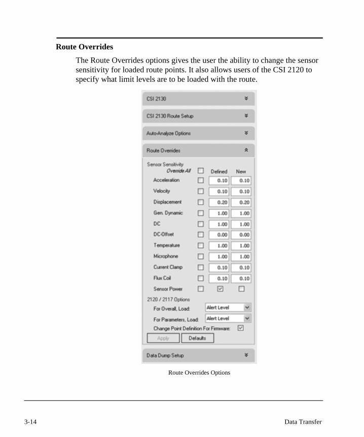
Route Overrides
The Route Overrides options gives the user the ability to change the sensor sensitivity for loaded route points. It also allows users of the CSI 2120 to specify what limit levels are to be loaded with the route.
Route Overrides Options
3-14 Data Transfer

In order to enable the override of a sensor sensitivity value, check the box next to the appropriate sensor type(s). Leave the checkbox(s) unchecked to leave the defined sensor sensitivity unchanged.
For each sensor type that is checked, enter in the “Defined” field the sensi-tivity value that is currently defined in the measurement point. Only sensitiv-ities of this value will be overridden. Then in the “New” field, enter the sensitivity that is to be loaded in place of that defined for the measurement point. If the user edits a “New” field, the check box for that sensitivity is auto-matically checked.
NoteThe enabled state of the override options are not saved across AMS Machinery Manager sessions. Therefore, the user will have to re-enable the override options upon each launch of AMS Machinery Manager. However, the values entered in the “Defined” and “New” fields are saved across the AMS Machinery Manager session.
Override All – This check box enables users to quickly enable or disable all sensor sensitivity overrides.
CSI 2120/CSI 2117 Options – These options only apply to routes loaded in the CSI 2120 or CSI 2117 analyzer. Since these analyzer’s are limited in the number of alarm level limits that may be loaded, the user can control which defined alarm level limits will be loaded. Separate control is provided for the Overall parameter and the defined Analysis Parameters.
For Overall, Load – There are four choices. The user can choose from the Alert Level, Warning Level, Fault Level, or the Lower of Warning or Alert. The Alert Level is the default selection. The specified value will become the overall alarm level for the loaded route.
For Parameters, Load – There are four choices. The user can choose from the Alert Level, Warning Level, Fault Level, or the Lower of Warning or Alert. The Alert Level is the default selection. The specified value will become the alarm level for the analysis parameters included in the loaded route.
3-15CSI 2130 Setup
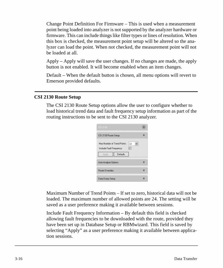
Change Point Definition For Firmware – This is used when a measurement point being loaded into analyzer is not supported by the analyzer hardware or firmware. This can include things like filter types or lines of resolution. When this box is checked, the measurement point setup will be altered so the ana-lyzer can load the point. When not checked, the measurement point will not be loaded at all.
Apply – Apply will save the user changes. If no changes are made, the apply button is not enabled. It will become enabled when an item changes.
Default – When the default button is chosen, all menu options will revert to Emerson provided defaults.
CSI 2130 Route Setup
The CSI 2130 Route Setup options allow the user to configure whether to load historical trend data and fault frequency setup information as part of the routing instructions to be sent to the CSI 2130 analyzer.
1
Maximum Number of Trend Points – If set to zero, historical data will not be loaded. The maximum number of allowed points are 24. The setting will be saved as a user preference making it available between sessions.
Include Fault Frequency Information – By default this field is checked allowing fault frequencies to be downloaded with the route, provided they have been set up in Database Setup or RBMwizard. This field is saved by selecting “Apply” as a user preference making it available between applica-tion sessions.
3-16 Data Transfer
CSI 2130 deviceIn order to upload and download from a CSI 2130 device, first launch AMS Machinery Manager and select the Data Transfer tab. In order to connect, make sure that the CSI 2130 analyzer is displayed in the “Enabled Devices” tab and the status shows “Waiting for connection”. See the section CSI 2130 Setup for further details. If communicating via USB, make sure the CSI USB Driver is installed.
If using USB communication, connect the USB cable from the analyzer to the local computer. Turn the analyzer on. On the analyzer screen, find and press the “Connect for Transfer” key. This will be on different menus depending on the program loaded and running in the analyzer. For more information, please see the CSI 2130 manual.
NoteThe connect key on the analyzer must be used before any com-munication can take place between the analyzer and computer.
3-17CSI 2130 Setup
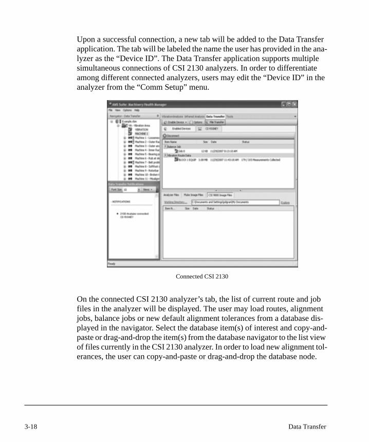
Upon a successful connection, a new tab will be added to the Data Transfer application. The tab will be labeled the name the user has provided in the ana-lyzer as the “Device ID”. The Data Transfer application supports multiple simultaneous connections of CSI 2130 analyzers. In order to differentiate among different connected analyzers, users may edit the “Device ID” in the analyzer from the “Comm Setup” menu.
Connected CSI 2130
On the connected CSI 2130 analyzer’s tab, the list of current route and job files in the analyzer will be displayed. The user may load routes, alignment jobs, balance jobs or new default alignment tolerances from a database dis-played in the navigator. Select the database item(s) of interest and copy-and-paste or drag-and-drop the item(s) from the database navigator to the list view of files currently in the CSI 2130 analyzer. In order to load new alignment tol-erances, the user can copy-and-paste or drag-and-drop the database node.
3-18 Data Transfer
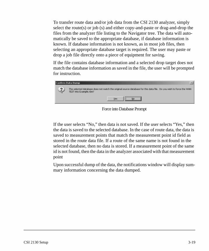
To transfer route data and/or job data from the CSI 2130 analyzer, simply select the route(s) or job (s) and either copy-and-paste or drag-and-drop the files from the analyzer file listing to the Navigator tree. The data will auto-matically be saved to the appropriate database, if database information is known. If database information is not known, as in most job files, then selecting an appropriate database target is required. The user may paste or drop a job file directly onto a piece of equipment for saving.
If the file contains database information and a selected drop target does not match the database information as saved in the file, the user will be prompted for instruction.
Force into Database Prompt
If the user selects “No,” then data is not saved. If the user selects “Yes,” then the data is saved to the selected database. In the case of route data, the data is saved to measurement points that match the measurement point id field as stored in the route data file. If a route of the same name is not found in the selected database, then no data is stored. If a measurement point of the same id is not found, then the data in the analyzer associated with that measurement point
Upon successful dump of the data, the notifications window will display sum-mary information concerning the data dumped.
3-19CSI 2130 Setup
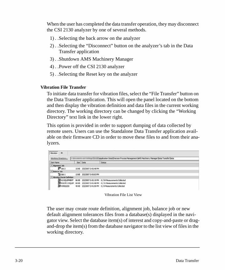
When the user has completed the data transfer operation, they may disconnect the CSI 2130 analyzer by one of several methods.
1) . .Selecting the back arrow on the analyzer2) . .Selecting the “Disconnect” button on the analyzer’s tab in the Data
Transfer application3) . .Shutdown AMS Machinery Manager4) . .Power off the CSI 2130 analyzer5) . .Selecting the Reset key on the analyzer
Vibration File TransferTo initiate data transfer for vibration files, select the “File Transfer” button on the Data Transfer application. This will open the panel located on the bottom and then display the vibration definition and data files in the current working directory. The working directory can be changed by clicking the “Working Directory” text link in the lower right.
This option is provided in order to support dumping of data collected by remote users. Users can use the Standalone Data Transfer application avail-able on their firmware CD in order to move these files to and from their ana-lyzers.
Vibration File List View
The user may create route definition, alignment job, balance job or new default alignment tolerances files from a database(s) displayed in the navi-gator view. Select the database item(s) of interest and copy-and-paste or drag-and-drop the item(s) from the database navigator to the list view of files in the working directory.
3-20 Data Transfer
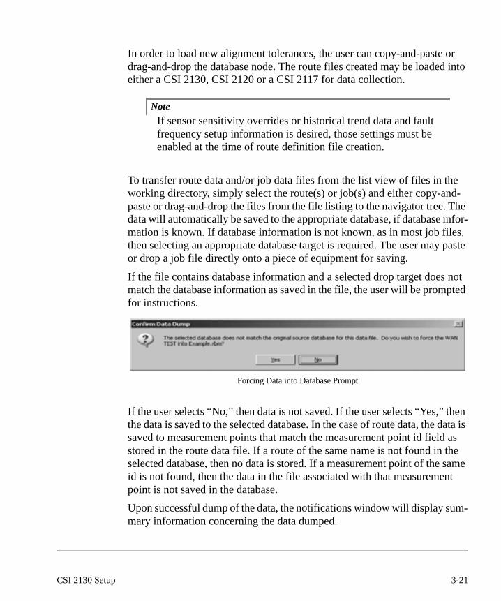
In order to load new alignment tolerances, the user can copy-and-paste or drag-and-drop the database node. The route files created may be loaded into either a CSI 2130, CSI 2120 or a CSI 2117 for data collection.
NoteIf sensor sensitivity overrides or historical trend data and fault frequency setup information is desired, those settings must be enabled at the time of route definition file creation.
To transfer route data and/or job data files from the list view of files in the working directory, simply select the route(s) or job(s) and either copy-and-paste or drag-and-drop the files from the file listing to the navigator tree. The data will automatically be saved to the appropriate database, if database infor-mation is known. If database information is not known, as in most job files, then selecting an appropriate database target is required. The user may paste or drop a job file directly onto a piece of equipment for saving.
If the file contains database information and a selected drop target does not match the database information as saved in the file, the user will be prompted for instructions.
Forcing Data into Database Prompt
If the user selects “No,” then data is not saved. If the user selects “Yes,” then the data is saved to the selected database. In the case of route data, the data is saved to measurement points that match the measurement point id field as stored in the route data file. If a route of the same name is not found in the selected database, then no data is stored. If a measurement point of the same id is not found, then the data in the file associated with that measurement point is not saved in the database.
Upon successful dump of the data, the notifications window will display sum-mary information concerning the data dumped.
3-21CSI 2130 Setup

If the auto-analyze option is enabled, the automatic analysis of the route data dumped will be performed at the completion of the save of the data.
3-22 Data Transfer

CSI 2130 PrintingIn order to print reports or plots from a CSI 2130 device, first launch AMS Machinery Manager and select the Data Transfer tab. In order to connect, make sure that the CSI 2130 analyzer is displayed in the “Enabled Devices” tab and the status shows “Waiting for connection.” See the section CSI 2130 Setup for further details. If communicating via USB, make sure the CSI USB Driver is installed.
If using USB communication, connect the USB cable from the analyzer to the local computer. Turn the analyzer on.
There are several ways available to connect the CSI 2130 analyzer for the print function. In the Route program, with a collected route active, the user may press the “ALT” key. This will display a “Print Route Report” option. From a plot display on the analyzer, the user may select the “Print Plot” option. For full information concerning the menu options in the CSI 2130 analyzer, please consult the analyzer manual.
Upon a successful connection, a new tab will be added to the Data Transfer application. The tab will be named the name the user has provided in the ana-lyzer as the “Device ID.” The Data Transfer application supports multiple simultaneous connections of CSI 2130 analyzers. In order to differentiate among different connected analyzers, users may edit the “Device ID” in the analyzer from the “Comm Setup” menu. For more information, please see the CSI 2130 manual.
As the host computer is receiving the report or plot pages from the analyzer, status will be updated in the printing control toolbar. The report or plot will not display until all pages have been received. This may take a long time for large reports.
The user may predetermine the output destination of received plots and reports via the drop-down “Destination” option on the printing toolbar. The user may choose any combination of “Screen,” “Printer,” or “File.” The default is “Screen.” In addition, the user may choose to automatically include either a new or previously saved cover page template to any received plots or reports via the same drop-down menu.
3-23CSI 2130 Printing

More than one report or plot may be displayed. To switch between reports, use the drop-down selection list in the printing toolbar.
Displayed reports or plots may be saved using the save button on the toolbar. Previously saved reports or plots may be opened using the open button on the toolbar. In order to print a displayed plot or report, select the print button. Page Setup options may be edited by selecting the page setup button on the toolbar.
Any plot or report may have a cover page added by selecting the “cover” drop down menu option. The user may create a new cover page or use a previously saved cover page template. The possible fields on the cover page include: Report Date, report type (i.e., Route, Job or Plot), Analyst, Company, Cus-tomer, Comments and a signature line. Every field except the Report Date and Report Type is customizable and removable. The image at the top of cover page may be changed as well.
3-24 Data Transfer

To edit the cover page of an already displayed report, double click on the dis-played cover page. The cover page edit dialog will be displayed. Use the menu option “Fields” to remove fields from the cover page. The user may directly type in the fields in the cover page displayed in the edit dialog. Right click on the cover page image to change or revert to Emerson provided default image on the cover page.
Printing Cover Page
3-25CSI 2130 Printing
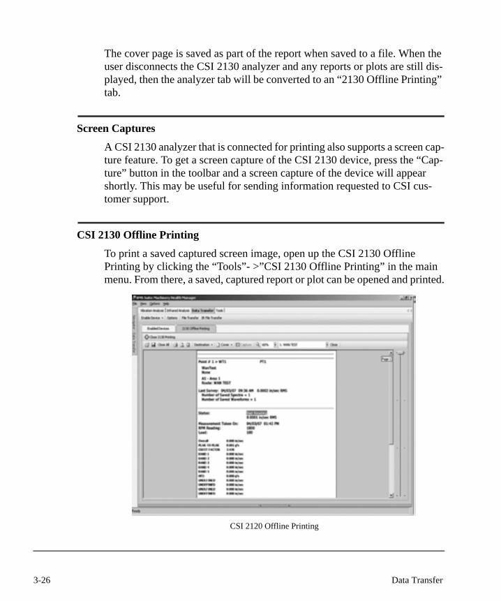
The cover page is saved as part of the report when saved to a file. When the user disconnects the CSI 2130 analyzer and any reports or plots are still dis-played, then the analyzer tab will be converted to an “2130 Offline Printing” tab.
Screen Captures
A CSI 2130 analyzer that is connected for printing also supports a screen cap-ture feature. To get a screen capture of the CSI 2130 device, press the “Cap-ture” button in the toolbar and a screen capture of the device will appear shortly. This may be useful for sending information requested to CSI cus-tomer support.
CSI 2130 Offline Printing
To print a saved captured screen image, open up the CSI 2130 Offline Printing by clicking the “Tools”- >”CSI 2130 Offline Printing” in the main menu. From there, a saved, captured report or plot can be opened and printed.
CSI 2120 Offline Printing
3-26 Data Transfer

Standalone Data Transfer ApplicationThe Standalone Data Transfer application is intended for use by remote users. It is not allowed to be installed on computers that have AMS Machinery Man-ager installed. It runs separately from the main application, AMS Machinery Manager. For this reason, it does not have the navigation tree that displays the database(s). The purpose of the Standalone Data Transfer application is to allow remote users to communicate for the purpose of loading and dumping with a CSI 2130, CSI 2120 or CSI 2117 analyzers. It will not load or dump routes or jobs from a database. It only allows the transfer of routes or jobs from the connected analyzer to a selected local file folder. In addition, it sup-ports updating firmware in a CSI 2130 and plot or report printing from a CSI 2130.
Those remote users may get the route definition files by either running AMS Machinery Manager in a Terminal Client session or be sent those route files by some other mechanism from a user that does have access to AMS Machinery Manager. The route data files are then retrieved from the ana-lyzers using the Standalone Data Transfer application. They can then be dumped to the database using AMS Machinery Manager in a Terminal Client session or sent to a user that does have access to AMS Machinery Manager for dumping and analysis.
Upon launch, the Standalone Data Transfer application will display the devices enabled for communication and a listing of vibration data files from the specified working directory. The working directory may be changed by selecting the “Working Directory…” button.
The bottom right side of the screen contains the notifications window. It will contain notifications or status information as to the state of the Data Transfer process. If an error occurs during processing or saving of data, it will be dis-played in this area as well.
3-27Standalone Data Transfer Application

Standalone Data Transfer Application
The communication setup options for the analyzers are the same as available in AMS Machinery Manager. Please see CSI 2130 Setup for communication setup options for the CSI 2130 analyzer.
Support of the CSI 2130 for file transfer and printing is the same as available via the AMS Machinery Manager version of Data Transfer. Please see section CSI 2130 Printing and Vibration File Transfer for details.
3-28 Data Transfer

Chapter 4
Cables and Adapters
Compatibility with the CSI 2130
Caution!Below is a chart of accessories compatible with the CSI 2130. Items not listed in the chart are not compatible with the CSI 2130. Using an accessory that is not supported may corrupt data. Please contact Product Support if you have any questions regarding an accessory’s compatibility with the CSI 2130.
Model # Description Comments
A649 Filter Headphone adapter without headphone, allows you to listen the vibration data as you collect.
DB25(MP or BNC accel inputs MS 2-pin “Lemo” connection
A648 Connects four accelerometers simultaneously; to use during a balancing job
DB25 to four each BNC connectors; channels are reversed from the 2120, but this does not impact balance jobs.
A639 Communications cable that attaches the analyzer to a computer
DB25 (M) to 9-pin (F)
A632 16-ft coiled sensor cable Lemo (M) DB25 (M)
Cable, DB25 to Lemo 6P, 16-ft straight cable
A632-S 632-S 16-ft grounded to analyzer cable; for use with a hand-held accelerometer
Cable, DB25 to Lemo 6P, 16-ft straight cable, grounded
A631 8-ft coil sensor cable Lemo (M) DB25 (M)
Cable, DB25 to Lemo 6P, 8-ft coil cable
4-1
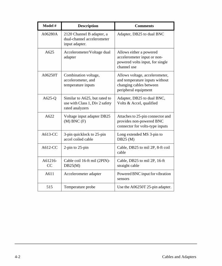
A06280A 2120 Channel B adapter, a dual-channel accelerometer input adapter.
Adapter, DB25 to dual BNC
A625 Accelerometer/Voltage dual adapter
Allows either a powered accelerometer input or non-powered volts input, for single channel use
A06250T Combination voltage, accelerometer, and temperature inputs
Allows voltage, accelerometer, and temperature inputs without changing cables between peripheral equipment
A625-Q Similar to A625, but rated to use with Class 1, Div 2 safety rated analyzers
Adapter, DB25 to dual BNC, Volts & Accel, qualified
A622 Voltage input adapter DB25 (M) BNC (F)
Attaches to 25-pin connector and provides non-powered BNC connector for volts-type inputs
A613-CC 3-pin quicklock to 25-pin accel coiled cable
Long extended MS 3-pin to DB25 (M)
A612-CC 2-pin to 25-pin Cable, DB25 to mil 2P, 8-ft coil cable
A61216-CC
Cable coil 16-ft mil (2PIN)-DB25(M)
Cable, DB25 to mil 2P, 16-ft straight cable
A611 Accelerometer adapter Powered BNC input for vibration sensors
515 Temperature probe Use the A06250T 25-pin adapter.
Model # Description Comments
4-2 Cables and Adapters

Optional Accessories for the CSI 2130
Model # Description Comments
A0684TX New integral-magnet triaxial sensor
Has the same wiring and connector as the A0614TX triax, and operates with both the 2120 and 2130, with the proper cable.
D24860 2130 Triaxial cable This cable is only compatible with the A0614TX triaxial accelerometer is not compatible with the A0643TX triaxial accelerometer.
D24861 2130 Tach input cable (6.56 ft) for the 404 infrared photo tach
Attaches the power/signal connector on the 404 tach cable to the 2130 tach/volts input (blue Turck connector).
D24862 2130 Tach input cable for generic tach (not the 404)
Attaches the standard BNC connector to the CSI 2130 tach/volts input cable (blue Turck connector).
D24863-1 18-in. SpeedVue cable Attaches the SpeedVue laser to the 2130 tach/volts input (blue Turck connector).
D24863-2 6-ft SpeedVue cable Attaches the SpeedVue laser to the 2130 tach/volts input (blue Turck connector).
A06290V 2130 dual-channel Volts input adapter
Attaches to the 25PIN connector on the 2130. This connector is blue to distinguish it from 2120 adapters. It will not work with the 2120.
D24859 Single-channel Volts input cable
Attaches a standard BNC connector to the CSI 2130 tach/volts input (blue Turck connector).
4-3
NoteConnect the D24860 triax cable directly to the CSI 2130 Turck accel input connector. The triax will not work if connected through the A06290A dual-channel Turck adapter.
NoteDo not use the older 25PIN triax cable for the 2120 with the CSI 2130 because the pins are different and confuse the X, Y, and Z channels.
NoteDo not use the 2120 buffered volts input adapters (A0623BF and A0628BV) with the CSI 2130. The CSI 2130 performs buffering internally.
4-4 Cables and Adapters
Chapter 5
Route
What is a Route?
A route groups measurement points on the equipment within an area in a con-venient order for data collection. A route is not a database, but it points to the equipment and measurement points within a database area.
Route Tips
• A route includes information from one area and is tagged to that area.• A route does not necessarily include every piece of equipment in an
area.• The order of equipment in a route can differ from its order in the data-
base area.• Equipment can appear in more than one route, but cannot appear in the
same route more than once.• The route measurement points do not necessarily include all points on
the equipment.• The route measurement points do not have to be in the same order as
listed for the equipment.• The route structure stores a list of equipment and measurement point
IDs as you define them when adding equipment to the route. During a route load, the software searches the area for the equipment and points that match the list. The equipment descriptions, speeds, measurement points and their definitions load into the analyzer. For this reason, the route does not recognize points if their IDs are modified in the data-base. Attempts to load the route causes errors.
• You can build and modify your routes in the Route Management pro-gram of AMS Machinery Manager.
5-1

Using a RouteThe simplest way to store data from a piece of equipment is to collect the data using a pre-defined route. Automated reporting and data plotting can be done by selecting a route of equipment to use.
NoteIf you have a single-channel 2130, you will not have all the Route features described in this section.
Collecting Data
The following paragraphs quickly describe a typical collection procedure after a route has been loaded into the analyzer and then selected.
1. . .Press Activate Route key to access the route, then use the Up/Down Arrow keys or the Equip List key to select and display the correct measurement point. (See “Route Data Collection: Measurement Point Display” on page 5-8.)
2. . .Place the sensor at the measurement point on the equipment, making sure that the sensor is in the correct plane.
3. . .Press Enter button or the Start Acq key to begin the measurement.4. . .The display will indicate that the analyzer is acquiring data. The
number of averages remaining displays on the screen until the measurement process is finished. Then the display indicates the overall value if analog overall has been selected.
5. . .Press the up arrow key to advance to the next measurement point and follow steps 2 through 4 above to continue data collection.
6. . .After a route has been completed, another route may be selected and the above procedure repeated. After a collection session, establish communications with the host computer and dump the collected data into the software database.
5-2 Route

To repeat a measurement, simply confirm that the correct measurement point is displayed and take the measurement again. If setup this way in the Data Storage Mode menu, the new data will replace the data that were collected in the last measurement.
NoteTo abort a measurement in progress, press the Reset key and then repeat the measurement.
NoteIf data has been collected on the wrong measurement point, press Clear Data key from the main menu to clear the most recent mea-surement data from the currently selected point. This procedure returns the measurement point to the “Not Measured” status.
Bad Sensor WarningWhen data collection begins on any point where the sensor power is turned on, the input signal is tested to verify proper sensor bias voltage. If the sensor or cable is not connected, or is electrically open or shorted, a bad sensor warning may appear.
Press the Enter button again to collect data anyway, or press the Back button to abort the measurement. The data will be marked as taken with a bad sensor. The Data Transfer application must be set up to accept bad sensor data before this data can be downloaded to the data base.
NoteA non-standard sensor or a measurement with extremely large vibration amplitudes may also trigger an erroneous warning.
Bad Reading Warning ...... indicates the value is above or below the valid signal setup defined in the measurement point setup in the database.
5-3Using a Route

Selecting Measurement PointsThere are three methods that can be used to select a measurement point from those in the current route. The first method is to simply scroll sequentially through the measurement points using the scroll keys or the Up/Down Arrow button. This is the usual procedure when following the order of measurement points in the route.
Jump to the first measurement point of the next or previous equipment (respectively) with the Left/Right Arrow button.
Equip List key lets you select equipment and associated measurement point. Press this key so that the Equip List screen displays all of the equipment within the current route. Scroll to highlight the desired equipment, and press the Enter button.
NoteA check appears before a point name on the Equipment List screen to indicate that data has been collected.
Making Dual-Channel Measurements (For Dual Channel version only)When making a dual-channel measurement in the normal Route mode, the analyzer must be displaying one of the two dual channel points. Press the Enter key to begin collecting data in the same manner as for a single channel. Data for both points are acquired at the same time.
Dual Channel and AMS Machinery Manager (For Dual Channel version only)In order to include dual-channel measurements on a normal route, the appli-cable measurement points must be set up as dual-channel points in the soft-ware.
The Measurement Point Information screen allows you to add dual channel points or to edit existing points to be defined as dual-channel. This screen is accessed from the Tree Structure option in the Database Setup/Management program. In a like manner, dual-channel points can be added when creating new equipment and their associated measurement points.
5-4 Route

A dual-channel measurement is set up as two individual measurement points that are grouped with the Signal Group field. Both points are defined with the same group number. One of the points is specified as Channel 1 and the other is specified as Channel 2. These data are collected on the A Channel and B Channel inputs, respectively. Both points must be on the same equipment; however, they do not necessarily have to be sequential in the point list.
Multiple Measurements from a Single SensorThe CSI 2130 can acquire data on two measurement points (even when the acquisition parameters are different) at the same time using one sensor con-nected to both channels.
The two measurement points are set up in the software as grouped points—the same way as regular dual points. However, define both points as Channel 1.
Data taken simultaneously on the same sensor will have the same date and time so both the software and the analyzer will allow you to display orbit plots. These plots are not true orbits since the data came from a single sensor.
5-5Using a Route

Route Data CollectionThe Route Data Collection Screen is the home screen for Route. From this screen you can:
• Take data• Change your measurement point or equipment• Add notes or field alerts to a point• Open the Analyze program.• Plot acquired data.
The Route Data Collection screen is the home screen for the Route program.
The alternate Route Data Collection screen lets you configure information that may influence your data. This includes:
• User Setup• Reset the sensitivity on a sensor
5-6 Route

• Set up a tachometer• Establish a new RPM• Print a Route Report
The Alternate Route Data Collection Screen.
You can also collect data from the alternate Route Data Collection screen. If you are ready to take data and your analyzer is set to the alternate screen, press Enter to begin data acquisition.
5-7Route Data Collection

Route Data Collection: Measurement Point Display
The Measurement Point display indicates the 2130 is in the normal route mode and ready to acquire data.
5-8 Route
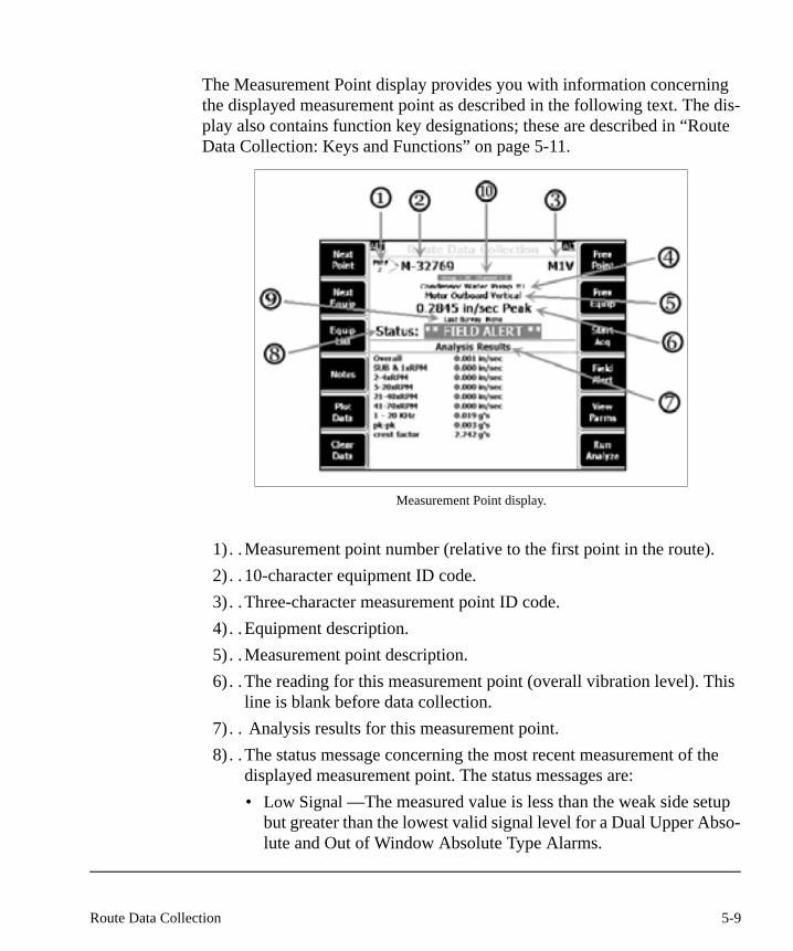
The Measurement Point display provides you with information concerning the displayed measurement point as described in the following text. The dis-play also contains function key designations; these are described in “Route Data Collection: Keys and Functions” on page 5-11.
Measurement Point display.
1) . .Measurement point number (relative to the first point in the route). 2) . . 10-character equipment ID code.3). .Three-character measurement point ID code.4). .Equipment description.5). .Measurement point description.6). .The reading for this measurement point (overall vibration level). This
line is blank before data collection. 7). . Analysis results for this measurement point.8). .The status message concerning the most recent measurement of the
displayed measurement point. The status messages are:• Low Signal —The measured value is less than the weak side setup
but greater than the lowest valid signal level for a Dual Upper Abso-lute and Out of Window Absolute Type Alarms.
5-9Route Data Collection

• High Signal – When using DL-A type alarms, high signal occurs when the signal is less than the upper validity limit of the sensor signal and greater than the weak side value. In DL-D type alarms the high signal can occur when the baseline value plus the weak side value has been exceeded but the value is still less than the upper sensor validity range.
• Warning – When using DU-A type alarms, Warning indicates that the baseline value has been exceeded but has not reached the Alert level.
• High Alarm 1 – The overall Alert value has been exceeded for Dual Upper Absolute and Out of Window Absolute Alarms.
• High Alarm 2 – The overall Fault value has been exceeded for Dual Upper Absolute and Out of Window Absolute Alarms.
• Window Alarm – The measured values are outside the valid alarm window, this occurs for an In Window Absolute Alarm. This is used when a parameter must stay outside a set range.
• Not Measured – No measurements have been made on this point. • OK – All measurements are within normal amplitude values
expected for this point. • Notes – Notes only has been added for this point. • Vib Alarm – One of the parameters has exceeded an alarm level. • Low Alarm 1 – For Dual Lower Delta type alarms, the Alarm occurs
when the baseline value minus the Alert value has been exceeded. For Dual Lower Absolute Alarms, the Alert value has been exceeded.
• Low Alarm 2 – For Dual Lower Delta type alarms, the Alarm occurs when the baseline value minus the Fault value has been exceeded. For Dual Lower Absolute Alarms, the Fault value has been exceeded.
• Bad Reading – The value is either lower or higher than the valid signal range setup for the point. Please check these setting from the point setup screen in the Dbase application.
5-10 Route

• Field Alert – The status line will only display this text if the user has enabled the Field Alert key (F10).
• Bad Sensor – When the route is loaded from the software, a sensor validity check is done on every measurement point. With sensor power turned ON in the point setup, the 2130 has to verify the sensor, cable and or adapter are all good. It is actually looking at the bias voltage of the accelerometer, if the voltage level is within a cer-tain window then the points are collected without any problems. If the voltage level is below or above a certain level then the message appears.
• When sensor power is OFF no checking is performed. • Out of Service – Equipment has been marked as out of service, no
data has been collected on any of the points. The Out of Service note will be transferred back to the database.
9). .Last Survey Date of data.10). Indicates the group/channel number of the current Measurement Point.
Route Data Collection: Keys and Functions
Next Point takes you to the next measurement point on a piece of equipment. The up arrow provides the same function. This key is also shown from the More Point Info screen. From this screen, the Up Arrow key will go to a next point.
Previous Point takes you to the last measurement point on a piece of equip-ment. The down arrow provides the same function. This key is also shown from the More Point Info screen. From this screen, the Down Arrow key will go to a previous point.
Next Equipment takes you to the next piece of equipment on a route. The right arrow provides the same function.
5-11Route Data Collection

Previous Equipment takes you to the first measurement point on the previous piece of equipment. The left arrow provides the same function.
Equipment List provides a list of all the equipment on a route on the top half of the screen and a list of all measurement points on the highlighted piece of equipment on the bottom half of the screen.
All equipment on the route is listed on the top half of the screen, while all the measurement points on the highlighted equipment are listed in the bottom half of the screen.
Activate Equipment brings the first point of the highlighted equipment to the Route Data Collection Screen.
Activate Point brings the highlighted measurement point on the equipment to the Route Data Collection Screen.
Next Unmeasured Point forwards you to the next measurement point with no data.
5-12 Route
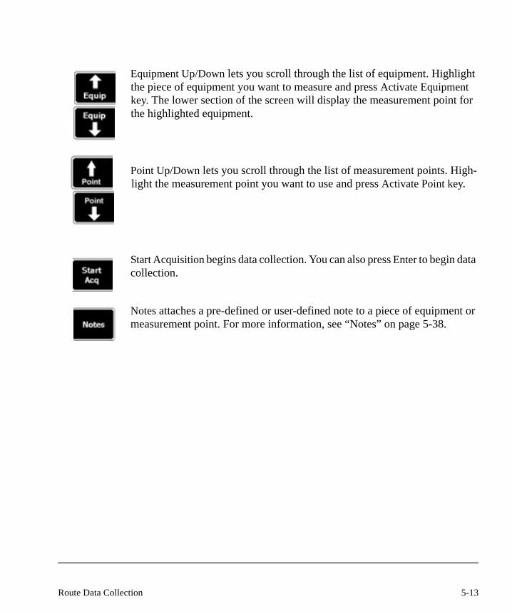
Equipment Up/Down lets you scroll through the list of equipment. Highlight the piece of equipment you want to measure and press Activate Equipment key. The lower section of the screen will display the measurement point for the highlighted equipment.
Point Up/Down lets you scroll through the list of measurement points. High-light the measurement point you want to use and press Activate Point key.
Start Acquisition begins data collection. You can also press Enter to begin data collection.
Notes attaches a pre-defined or user-defined note to a piece of equipment or measurement point. For more information, see “Notes” on page 5-38.
5-13Route Data Collection
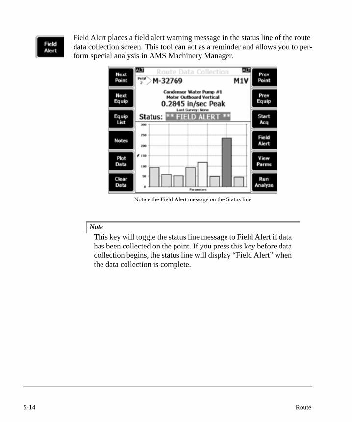
Field Alert places a field alert warning message in the status line of the route data collection screen. This tool can act as a reminder and allows you to per-form special analysis in AMS Machinery Manager.
Notice the Field Alert message on the Status line
NoteThis key will toggle the status line message to Field Alert if data has been collected on the point. If you press this key before data collection begins, the status line will display “Field Alert” when the data collection is complete.
5-14 Route

Plot Data takes you to the plot function screen. This feature is only available if you have collected data. While viewing the spectrum plot any optional fault frequency information downloaded with route may be viewed.
Plot Function Screen with Next Fault Frequency Key
NoteIf the input has been configured as a gearbox with multiple shafts, all the information may not display on the plot due to lim-ited space. The information can be seen by pressing the F1 key; the exact fault frequency will be high lighted in the entry list and a check mark placed beside the fault ID.
5-15Route Data Collection

Fault Frequenciese
NoteThe ID and description are the fault associated with the fault fre-quency entry. Example from image above: A, B, C, D and asso-ciated with SKF 1200.
Next Fault Freq will start at the beginning of the fault entry list. If multiple fault frequency entries are shown, then the key will progress through the entries in a sequential order, from top to bottom.
If a single fault ID has been added to the plot from the fault frequency list key; then pressing this key will clear the previous fault ID and replace it with the next fault ID from the list.
If multiple fault IDs have been added to the plot from the fault frequency list key; then pressing this key will clear the plot and replace it with the first fault ID from the list.
5-16 Route

Prev Fault Freq will start at the bottom of the fault entry list. If multiple fault frequency entries are shown: then the key will progress through the entries in reverse order, from bottom to top.
If a single fault ID has been added to the plot from the fault frequency list key; then pressing this key will clear the fault ID and replace it with the previous fault ID from the list.
If multiple fault IDs have been added to the plot from the fault frequency list key; then pressing this key will clear the plot and replace it with the last fault ID from the list.
View Parameters shows a list of all parameters set up from the AP set. This screen is shown with the measured value and percent (%) of alarm.
Run Analyze opens the Analyze program. See chapter 8 for more information about Analyze.
Clear Data clears data from the Route point. A dialog box appears asking if you want to do this. Press the Enter button if you want to delete the data or press the Back button if you do not.
5-17Route Data Collection

NoteIf multiple data sets are stored on the Route point, the user will have to select which set of data to delete. Use the Data Up and Down keys to select your data point. Then press the Delete Data Set key.
Screen showing multiple data sets on one Route point.
5-18 Route
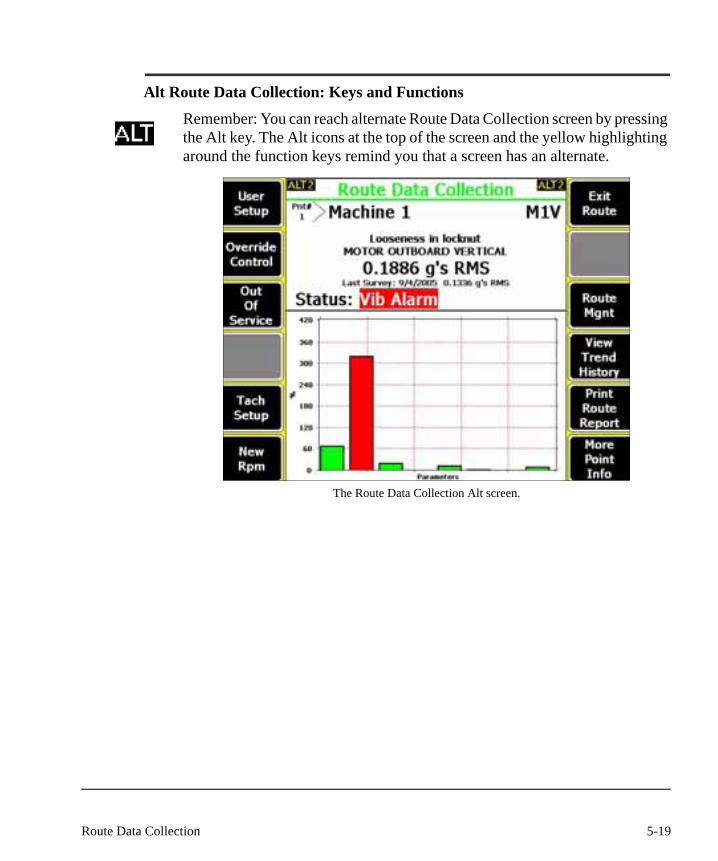
Alt Route Data Collection: Keys and Functions
Remember: You can reach alternate Route Data Collection screen by pressing the Alt key. The Alt icons at the top of the screen and the yellow highlighting around the function keys remind you that a screen has an alternate.
The Route Data Collection Alt screen.
5-19Route Data Collection
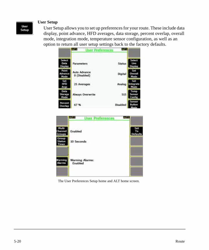
User SetupUser Setup allows you to set up preferences for your route. These include data display, point advance, HFD averages, data storage, percent overlap, overall mode, integration mode, temperature sensor configuration, as well as an option to return all user setup settings back to the factory defaults.
The User Preferences Setup home and ALT home screen.
5-20 Route
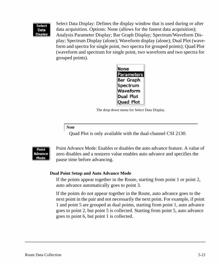
Select Data Display: Defines the display window that is used during or after data acquisition. Options: None (allows for the fastest data acquisition); Analysis Parameter Display; Bar Graph Display; Spectrum/Waveform Dis-play; Spectrum Display (alone); Waveform display (alone); Dual Plot (wave-form and spectra for single point, two spectra for grouped points); Quad Plot (waveform and spectrum for single point, two waveform and two spectra for grouped points).
The drop down menu for Select Data Display.
NoteQuad Plot is only available with the dual-channel CSI 2130.
Point Advance Mode: Enables or disables the auto advance feature. A value of zero disables and a nonzero value enables auto advance and specifies the pause time before advancing.
Dual Point Setup and Auto Advance ModeIf the points appear together in the Route, starting from point 1 or point 2, auto advance automatically goes to point 3.
If the points do not appear together in the Route, auto advance goes to the next point in the pair and not necessarily the next point. For example, if point 1 and point 5 are grouped as dual points, starting from point 1, auto advance goes to point 2, but point 5 is collected. Starting from point 5, auto advance goes to point 6, but point 1 is collected.
5-21Route Data Collection

Set HFD Averages: Opens a box where you can change the High Frequency Detection (HFD) averages. You can choose between one and 99 averages.
HFD is the amplitude of vibration in g's over a broad frequency band from 5 kHz to 20 kHz. Collected vibration data with energy between 5 kHz to 20 kHz is computed.
Choose the number of averages for High Frequency Detection.
NoteThe HFD parameters are set up from the Analysis Parameter Set information in the DBase application from the software.
Data Storage Mode: Select how data is stored for a route. There are three modes:
Always Overwrite: Stores one set of route data per point. It over-writes any old material automatically.
Query Overwrite: Stores only one set of route data per point. It asks your permission before overwriting data.
Store All Data: Adds new route data to the old data stored on a measurement point. This mode allows multiple sets of data to be collected before the Route data is dumped to the software.
NoteContinuously adding Route data to the data file makes the data file very large and could affect the performance of the analyzer. The Route data should be deleted periodically after it has been dumped.
5-22 Route
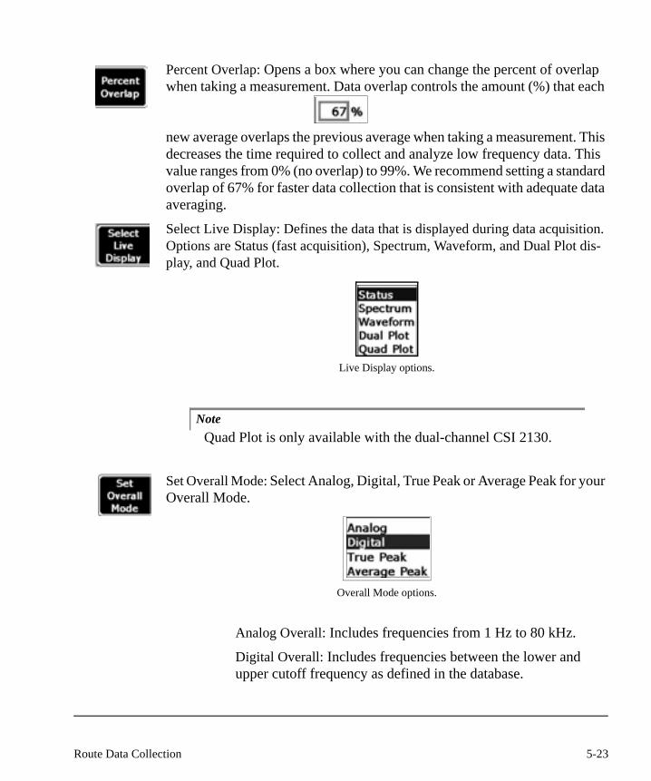
Percent Overlap: Opens a box where you can change the percent of overlap when taking a measurement. Data overlap controls the amount (%) that each
new average overlaps the previous average when taking a measurement. This decreases the time required to collect and analyze low frequency data. This value ranges from 0% (no overlap) to 99%. We recommend setting a standard overlap of 67% for faster data collection that is consistent with adequate data averaging.
Select Live Display: Defines the data that is displayed during data acquisition. Options are Status (fast acquisition), Spectrum, Waveform, and Dual Plot dis-play, and Quad Plot.
Live Display options.
NoteQuad Plot is only available with the dual-channel CSI 2130.
Set Overall Mode: Select Analog, Digital, True Peak or Average Peak for your Overall Mode.
Overall Mode options.
Analog Overall: Includes frequencies from 1 Hz to 80 kHz.
Digital Overall: Includes frequencies between the lower and upper cutoff frequency as defined in the database.
5-23Route Data Collection

True Peak: Is obtained from the waveform. As all data is col-lected, the meter remembers the highest and lowest peaks from the entire collection period. The meter takes this total value and divides it by two.
Average Peak: Is obtained from the waveform. As each waveform is collected, the meter records the highest and lowest value from anywhere within the block and divides this value by two. After all blocks are collected, the meter averages these individual peak values to calculate the final Average Peak.
NoteThese settings can be overridden in the software. If the settings for Overall and Integration are different than those in the ana-lyzer, those in the software will be used.
Set Integrate Mode: Allows you to choose Digital or Analog for your Integrate Mode. The default setting is Analog. The same feature is available in the Ana-lyze program.
Choose Analog or Digital for your Integrate Mode.
• Analog Integration – When Analog is selected, the waveform data is integrated and then the FFT is performed. The end result is that the waveform and spectrum are stored in the integrated units. Analog inte-gration generally provides more accuracy and less low frequency noise.
• Digital Integration – When Digital is selected, the FFT is performed first and then the integration is performed on the spectrum. The end result is that the waveform is stored in the sensor units and the spec-trum is stored in the integrated units.
5-24 Route

Temperature Sensor Configuration: Choose Generic for any sensor with an output voltage proportional to the temperature, or select 515 if you are using the 515 sensor from Emerson.
Choose Generic or a specific sensor for your Temperature Sensor configuration
Note515 is the default setting.
Sensor Button Mode: Toggles through Disabled, Enter Only, and Enter/Advance. Disabled means this feature is disabled. In the Enter Only mode the Sensor Button Mode key functions as the Enter key. In the Enter/Advance mode, the sensor button starts data collection if no data has been collected on the cur-rent point. Or, it advances to the next point if data has already been collected on the current point.
NoteThis feature should only be used with the model A350-1 accel-erometer.
Multi Channel Groups: This allows the multi-channel group data collection to be enabled or disabled. This feature is normally enabled and should only be dis-abled if the route cannot be collected in the current state. An example would be a route that is set to use a triaxial accelerometer, but the sensor is not available.
NoteWhen the groups are un-linked, all data is collected on Channel A.
5-25Route Data Collection
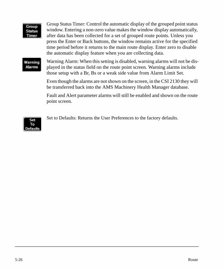
Group Status Timer: Control the automatic display of the grouped point status window. Entering a non-zero value makes the window display automatically, after data has been collected for a set of grouped route points. Unless you press the Enter or Back buttons, the window remains active for the specified time period before it returns to the main route display. Enter zero to disable the automatic display feature when you are collecting data.
Warning Alarm: When this setting is disabled, warning alarms will not be dis-played in the status field on the route point screen. Warning alarms include those setup with a Br, Bs or a weak side value from Alarm Limit Set.
Even though the alarms are not shown on the screen, in the CSI 2130 they will be transferred back into the AMS Machinery Health Manager database.
Fault and Alert parameter alarms will still be enabled and shown on the route point screen.
Set to Defaults: Returns the User Preferences to the factory defaults.
5-26 Route

Override ControlIf you need to swap sensors while you are collecting data, you may need to adjust the sensitivity setting in your analyzer. Press the Override Control key in the Route Data Collection screen to open the Override menu. Scroll through a list of available sensors. Highlight the type of sensor you are using, then adjust the sensitivity using the active buttons. Press enter to return to the Route Data Collection screen.
The Conversion Override table.
Sensor Sensitivity Override: Lets you enable or disable the sensitivity substi-tution for the sensor types.
Set Defined Sensitivity: The value defined in the measurement point setup
Set New Sensitivity: If the sensor sensitivity is enabled, enter a new value into this field to override the defined value. This becomes the new sensitivity for the selected sensor.
Sensor Power Override: Enable if you want the new sensor power to override the defined sensor power.
Define Sensor Power: If sensor power override is enabled, all points matching the defined sensor power setting use the new sensor power setting instead.
5-27Route Data Collection
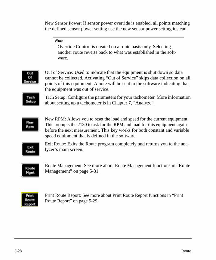
New Sensor Power: If sensor power override is enabled, all points matching the defined sensor power setting use the new sensor power setting instead.
NoteOverride Control is created on a route basis only. Selecting another route reverts back to what was established in the soft-ware.
Out of Service: Used to indicate that the equipment is shut down so data cannot be collected. Activating “Out of Service” skips data collection on all points of this equipment. A note will be sent to the software indicating that the equipment was out of service.
Tach Setup: Configure the parameters for your tachometer. More information about setting up a tachometer is in Chapter 7, “Analyze”.
New RPM: Allows you to reset the load and speed for the current equipment. This prompts the 2130 to ask for the RPM and load for this equipment again before the next measurement. This key works for both constant and variable speed equipment that is defined in the software.
Exit Route: Exits the Route program completely and returns you to the ana-lyzer’s main screen.
Route Management: See more about Route Management functions in “Route Management” on page 5-31.
Print Route Report: See more about Print Route Report functions in “Print Route Report” on page 5-29.
5-28 Route

More Point Info: Press this key to get detailed information from the measure-ment point and analysis parameter setup screens from the database.
More Point Info screen
Sensor Setup: Shows the sensor setup for the current route point.
View dB Ref: Displays the dB references values for the current route.
Show Group Status: Displays the status summary for all points that belong to the current group. Information about the equipment, group, and measurement points is displayed. Activate this window manually from the Point Informa-tion screen, or automatically from the Measurement Point screen (after col-lecting route data for a set of grouped points.
5-29Route Data Collection

NoteAutomatic display occurs only if the Group Status Time value is greater than zero. See Group Status Time in User Setup for more information.
NoteThe Show Group Status key is left blank if the current measure-ment point is not part of a group.
Group Status screen
Measurement Up/Down: Scrolls through measurement points in the list. High-light a point and press Enter to activate it.
5-30 Route
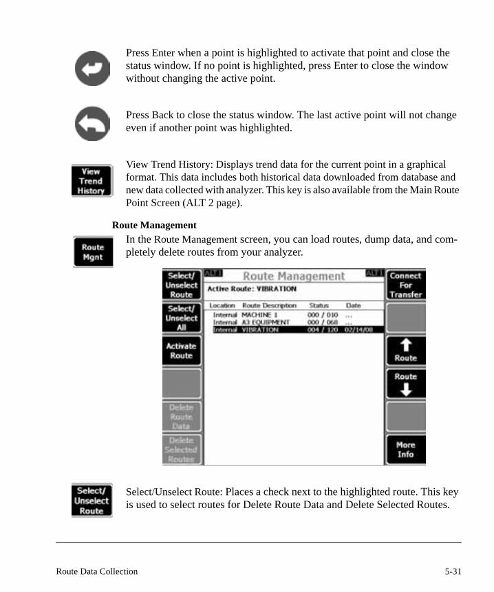
Press Enter when a point is highlighted to activate that point and close the status window. If no point is highlighted, press Enter to close the window without changing the active point.
Press Back to close the status window. The last active point will not change even if another point was highlighted.
View Trend History: Displays trend data for the current point in a graphical format. This data includes both historical data downloaded from database and new data collected with analyzer. This key is also available from the Main Route Point Screen (ALT 2 page).
Route ManagementIn the Route Management screen, you can load routes, dump data, and com-pletely delete routes from your analyzer.
1
Select/Unselect Route: Places a check next to the highlighted route. This key is used to select routes for Delete Route Data and Delete Selected Routes.
5-31Route Data Collection

Unselect All Routes: Deselects all the routes from the Route Management screen.
Activate Route: Highlight the route you want to use and press Activate Route to return to the Route Data Collection screen and begin using the route.
More Info: Press to learn more information about the route loaded on the ana-lyzer.
More Info dialog box
Select All Routes: Selects all the routes from the Route Management screen. Use this key to delete route data only or to delete all routes loaded.
Connect for Transfer: Connects you to your PC and Data Transfer for loading and dumping information.
5-32 Route
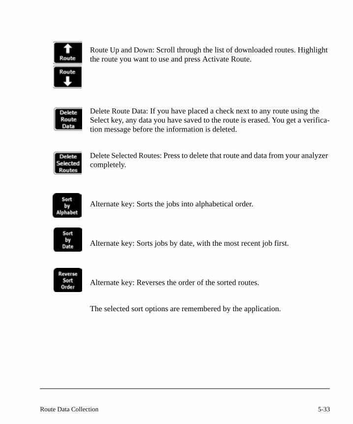
Route Up and Down: Scroll through the list of downloaded routes. Highlight the route you want to use and press Activate Route.
Delete Route Data: If you have placed a check next to any route using the Select key, any data you have saved to the route is erased. You get a verifica-tion message before the information is deleted.
Delete Selected Routes: Press to delete that route and data from your analyzer completely.
Alternate key: Sorts the jobs into alphabetical order.
Alternate key: Sorts jobs by date, with the most recent job first.
Alternate key: Reverses the order of the sorted routes.
The selected sort options are remembered by the application.
5-33Route Data Collection
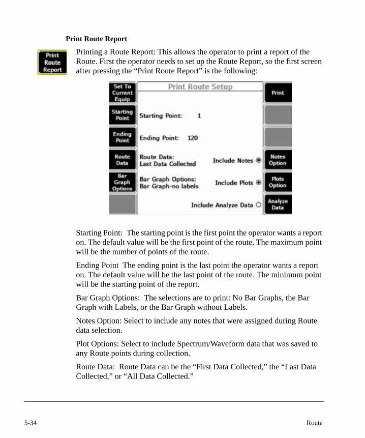
Print Route Report
Printing a Route Report: This allows the operator to print a report of the Route. First the operator needs to set up the Route Report, so the first screen after pressing the “Print Route Report” is the following:
2
Starting Point: The starting point is the first point the operator wants a report on. The default value will be the first point of the route. The maximum point will be the number of points of the route.
Ending Point The ending point is the last point the operator wants a report on. The default value will be the last point of the route. The minimum point will be the starting point of the report.
Bar Graph Options: The selections are to print: No Bar Graphs, the Bar Graph with Labels, or the Bar Graph without Labels.
Notes Option: Select to include any notes that were assigned during Route data selection.
Plot Options: Select to include Spectrum/Waveform data that was saved to any Route points during collection.
Route Data: Route Data can be the “First Data Collected,” the “Last Data Collected,” or “All Data Collected.”
5-34 Route

Analyze Data: Additional Analyze data that was saved to Route points during the Route Collection can also be printed. The operator can choose to either have the Analyze Data included or not included.
Print: The Print key or the Enter key will start printing of the Route Report.
An example of a Route Report for a single point is shown.
5-35Route Data Collection

5-36 Route
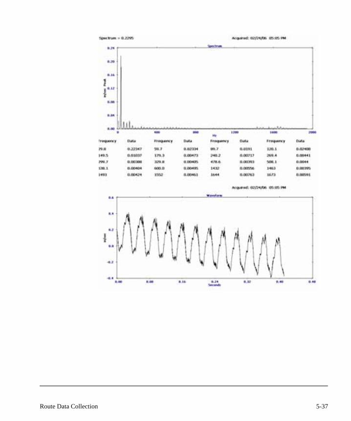
3
5-37Route Data Collection
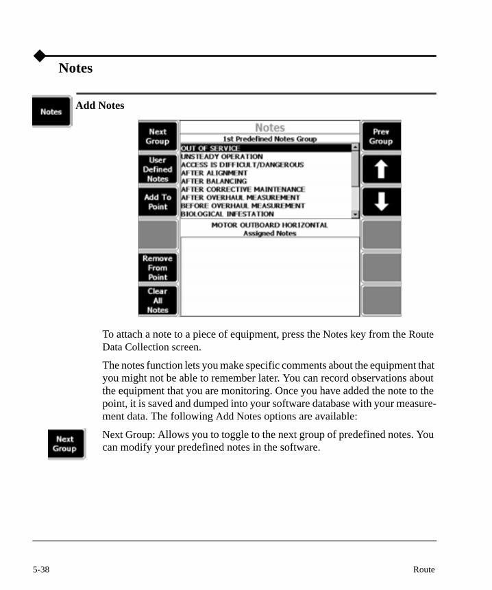
Notes
Add Notes
4
To attach a note to a piece of equipment, press the Notes key from the Route Data Collection screen.
The notes function lets you make specific comments about the equipment that you might not be able to remember later. You can record observations about the equipment that you are monitoring. Once you have added the note to the point, it is saved and dumped into your software database with your measure-ment data. The following Add Notes options are available:
Next Group: Allows you to toggle to the next group of predefined notes. You can modify your predefined notes in the software.
5-38 Route
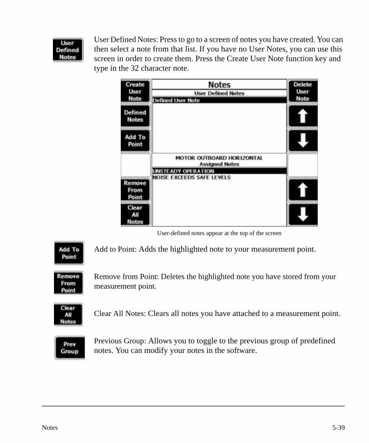
User Defined Notes: Press to go to a screen of notes you have created. You can then select a note from that list. If you have no User Notes, you can use this screen in order to create them. Press the Create User Note function key and type in the 32 character note.
User-defined notes appear at the top of the screen
Add to Point: Adds the highlighted note to your measurement point.
Remove from Point: Deletes the highlighted note you have stored from your measurement point.
Clear All Notes: Clears all notes you have attached to a measurement point.
Previous Group: Allows you to toggle to the previous group of predefined notes. You can modify your notes in the software.
5-39Notes

Up/Down Arrows: Allow you to scroll through the list of predefined notes or the list of stored notes on a measurement point.
5-40 Route
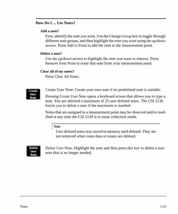
How Do I ... Use Notes?
Add a note?First, identify the note you want. Use the Change Group key to toggle through different note groups, and then highlight the note you want using the up/down arrows. Press Add to Point to add the note to the measurement point.
Delete a note?Use the up/down arrows to highlight the note you want to remove. Press Remove from Point to erase that note from your measurement point.
Clear all of my notes?Press Clear All Notes.
Create User Note: Create your own note if no predefined note is suitable.
Pressing Create User Note opens a keyboard screen that allows you to type a note. You are allowed a maximum of 25 user-defined notes. The CSI 2130 forces you to delete a note if the maximum is reached.
Notes that are assigned to a measurement point may be observed and/or mod-ified at any time the CSI 2130 is in route collection mode.
NoteUser defined notes stay stored in memory until deleted. They are not removed when route data or routes are deleted.
Delete User Note: Highlight the note and then press this key to delete a user note that is no longer needed.
5-41Notes
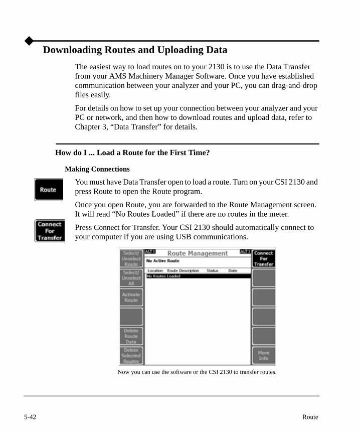
Downloading Routes and Uploading DataThe easiest way to load routes on to your 2130 is to use the Data Transfer from your AMS Machinery Manager Software. Once you have established communication between your analyzer and your PC, you can drag-and-drop files easily.
For details on how to set up your connection between your analyzer and your PC or network, and then how to download routes and upload data, refer to Chapter 3, “Data Transfer” for details.
How do I ... Load a Route for the First Time?
Making Connections
You must have Data Transfer open to load a route. Turn on your CSI 2130 and press Route to open the Route program.
Once you open Route, you are forwarded to the Route Management screen. It will read “No Routes Loaded” if there are no routes in the meter.
Press Connect for Transfer. Your CSI 2130 should automatically connect to your computer if you are using USB communications.
Now you can use the software or the CSI 2130 to transfer routes.
5-42 Route

Load a Route using Data TransferExpand the database tree and then expand the areas to get to the route level. Drag and drop the files you need from under the computer graphic to under the CSI 2130 graphic.
Load a Route using the CSI 2130
Connect the CSI 2130 to the computer to load routes.
Press Set Storage Location to toggle through the list of places where you can save your routes. Choose from Internal, Card, or Card 2).
NoteIf the version of the 2130 you have has only one card slot, you will not have the Card 2 option.
NoteA USB drive plugged in cannot be selected as a storage location from within an application.
5-43Downloading Routes and Uploading Data

Once you have chosen a storage location, press Load Routes. The database names appear at the top of the screen. Areas within each database appear at the bottom. Highlight the database you want to use, and select the area you need.
Highlight the database at the top of the screen, then highlight the area at the bottom.
Highlight each route you want to load and press Select. Press Load Route to load the routes you have selected.
Press Select and check the highlighted route to load onto your CSI 2130.
5-44 Route
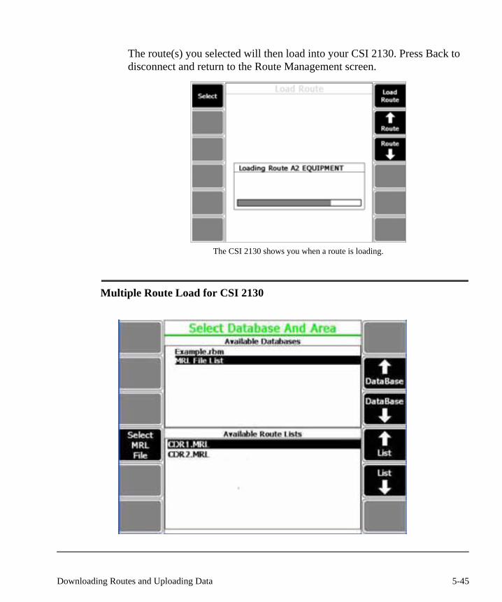
The route(s) you selected will then load into your CSI 2130. Press Back to disconnect and return to the Route Management screen.
The CSI 2130 shows you when a route is loading.
Multiple Route Load for CSI 2130
5-45Downloading Routes and Uploading Data

Multiple Route Load (MRL) allows Routes from multiple databases to be grouped into one file (.mrl). If these files have been previously set-up in the software, then the “MRL File List” will appear at the database level. Select the MRL from the list window to load all routes into the CSI 2130.
NoteMRL files are created from within the Route Management appli-cation.
What if I’ve Already Loaded a Route?If you have routes loaded in your CSI 2130, you may be forwarded to the Route Data Collection screen when you open the Route Program. If you want to add new routes, press ALT on the Route Data Collection Screen and then press Route Mgnt.
If you try to load a route with the same filename as a route that is already loaded into the CSI 2130, you get this error message:
You get an error message if you download a route that has the same filename as a route that is already loaded into the CSI 2130.
If you press Enter from this screen to continue, you will replace your old route with the new route and will loose all data.
5-46 Route

NoteThe above message will be shown when loading the same route to the same memory location. The same route can be loaded to the internal memory and external storage card.
5-47Downloading Routes and Uploading Data
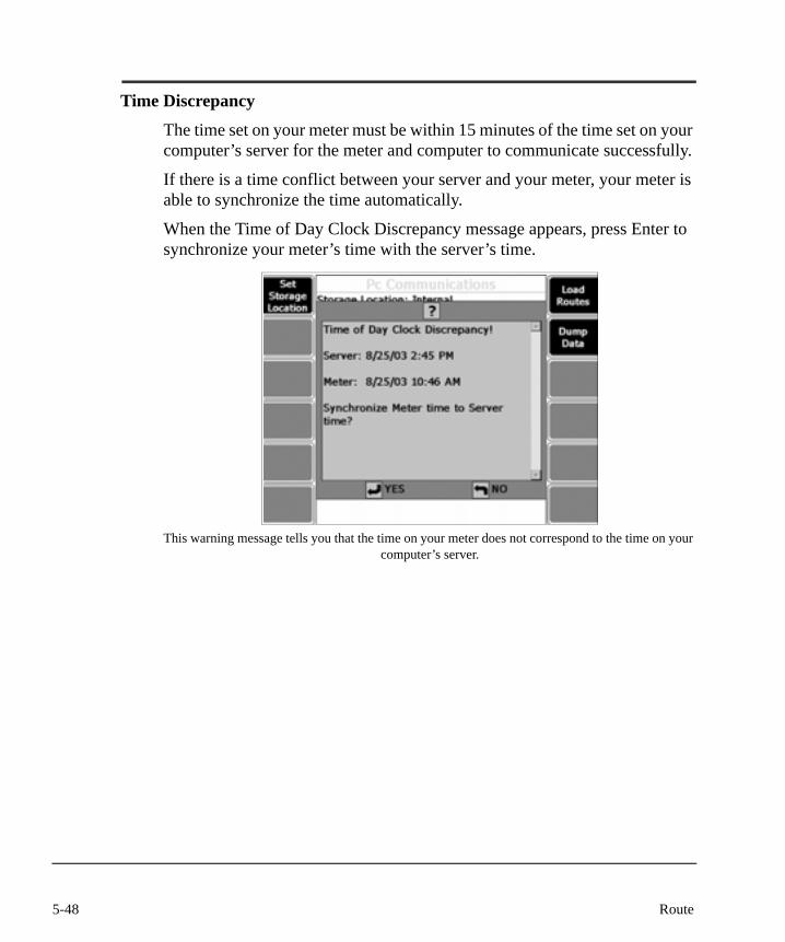
Time Discrepancy
The time set on your meter must be within 15 minutes of the time set on your computer’s server for the meter and computer to communicate successfully.
If there is a time conflict between your server and your meter, your meter is able to synchronize the time automatically.
When the Time of Day Clock Discrepancy message appears, press Enter to synchronize your meter’s time with the server’s time.
This warning message tells you that the time on your meter does not correspond to the time on your computer’s server.
5-48 Route
Chapter 6
Analysis Experts
Running the Experts The Experts perform best if you collect data and mark a frequency of interest in the spectrum before you run the test.
Selecting Analysis Experts:• Each Expert uses predefined settings for acquiring data if no measure-
ment point is defined.• If a route measurement point is active (even if data has not been col-
lected on the point), the Expert uses the setup information from the existing point to perform a customized acquisition.
• If data is collected and a cursor marks a certain frequency, the Expert performs a customized acquisition based on the marked frequency and other point setup information. Select the Expert immediately after marking the frequency—before you press the Reset key or move to another measurement point.
6-1

Analysis Experts
Analysis Experts on the main Analyze Application screen
High Frequency AnalysisUse this expert to acquire data beyond the standard maximum frequency of the route point or marked spectra.
Use High Frequency Analysis when there are a lot of peaks on the right hand side of the spectrum, or when a high frequency band such as HFD is in alarm.
High Resolution AnalysisUse the high-resolution analysis test to increase the resolution of spectral data. Increasing the spectral data is useful for separating closely spaced peaks. This expert acquires data with better resolution than the standard route or marked spectra.
6-2 Analysis Experts
For example: In a 3600 RPM motor, it can be difficult to distinguish vibration from two times the turning speed (misalignment) from two times the line fre-quency (120 Hz, electrical problem). If you see a high-amplitude vibration peak near 7200 CPM in the route spectrum, use the high-resolution expert to zoom in and separate the two frequencies. You may also use this feature to distinguish closely spaced sideband frequencies for rotor bar or gear mesh problems.
• If data has already been collected on the measurement point, the expert increases the resolution based on the original resolution setting.
• If you mark a frequency of interest in the spectrum before beginning the test, the expert applies increased resolution or zoom analysis to the specific frequency area.
• If you mark a frequency again and repeat the measurement, the resolu-tion increases each time until the analyzer is unable to provide addi-tional lines of resolution. Be aware that as resolution increases, it is possible for the test to take a long time to collect the data. For example, the test would take over 10 minutes if the Fmax is set at 10 Hz (600 CPM) with 6400 lines of resolution.
Bearing/Gear Analysis - PeakVueThis patented processing technique detects anti-friction bearing or gear defects at an earlier stage than normal vibration measurements. It also detects bearing defects on extremely slow turning shafts that do not generate enough vibration to be detected with normal measurements.
Due to the short duration of bearing impacts, a higher frequency sensor with an Fmax set between 10,0000 and 15,0000 Hz works best, even if you mea-sure slow speed machines. Place the sensor in the radial (horizontal) or axial position as near to the load zone of the bearing as possible, and on a very flat surface (without paint if possible).
Bearing defect frequencies appear in the PeakVue spectrum, just as they would in a normal spectrum, at their fundamental frequencies and harmonics. These peaks are non-synchronous. Gear defects appear as peaks at the gear’s shaft turning speed frequency and harmonics. PeakVue waveform data is cor-rected so that all spikes in the data are displayed on the positive side of the waveform. The amplitude of spikes in the waveform is an absolute measure-ment and determines the severity of impacting.
6-3
• If data has already been collected on the measurement point, the Expert starts with the original acquisition settings and adds the PeakVue pro-cessing.
• A variation: Set a new, lower Fmax for the PeakVue measurement if the original spectrum shows no vibration peaks past a certain fre-quency. To do this, mark the cursor to the right of the last vibration peak; then select the PeakVue expert. The Fmax of the new spectrum is lowered to the next available Fmax setting in the analyzer, above the marked frequency.
Application: PeakVue removes normal vibration signals and captures the actual amplitude of high frequency impacting from bearing or gear defects.
NoteMount the sensor on a stud or magnet and on a clean, flat surface (no paint if possible).
Low Frequency Analysis - Slow Speed Technology (SST)This test applies Slow Speed Technology (SST) processing and acquires data to help detect problems with low speed equipment. Use it to look at very low speed data (usually below 10 Hz) that has been integrated from acceleration to velocity or displacement. The SST process enhances the low frequency data by removing the “ski-slope” effect, and correcting the amplitude values of vibration peaks. For low frequency measurements, a special low frequency accelerometer is recommended, but SST works with a standard sensor as well.
The data is interpreted the same as regular spectra. A high amount of resolu-tion is used so that the harmonics of the very low fundamental frequencies are separated at very low frequencies.
• The Expert considers the original acquisition settings when it deter-mines the low frequency analysis settings, if data has been collected on the measurement point.
• If you mark a low frequency peak of interest in the spectrum before beginning the test, the Expert uses that frequency and sets the new Fmax equal to or just above the marked frequency.
6-4 Analysis Experts
Turning Speed DetectionUse this expert to confirm shaft-turning speed. This test confirms the shaft turning speed frequency. After you press the Enter key, type in the shaft turning speed you suspect and press Enter. The test collects a spectrum and detects the largest peak closest to that speed. The dominate peak nearest the suspected turning speed frequency is most likely the turning speed.
The turning speed detection expert is also available when you collect data on a variable-speed machine. When the analyzer prompts you, enter the machine RPM.
A spectrum is collected and displayed with a cursor that marks the turning speed peak. Press the Set RPM function key before pressing the Enter key and the analyzer accepts the new RPM value. If you do not press the Set RPM key, the analyzer uses the original RPM value.
Laser Speed DetectionUse this expert to confirm shaft-turning speed.
Using the Model 430 laser speed sensor, connect the speed sensor to the tach input and turn it on. Turn the sensor off when you are not using it.
If you use the Model 430 laser speed sensor with no route loaded, select the RPM range from the menu and press the Enter key.
NoteIf the tach power is turned off from the Tach menu in Manual Analyze, you can leave the switch for the speed sensor on. Selecting this expert automatically turns the power on for the Model 430 and turns the laser beam off after the reading is com-pleted. If the tach power is on and the switch is on, the Model 430 will stay on continuously.
6-5

Press the More Experts function key to reach the other Analysis Experts.
More Analysis Experts on the Analyze Application screen
Bump Test Equipment OffUse this test to check for resonance when high vibration is otherwise unex-plained. The spectrum may show a broad hump of energy or a single discrete peak. You want to determine if the high amplitude of a frequency is caused by high input force or low input force that is amplified by resonance
For best results with this type of test, turn off the machine in question. This is because the operational vibration amplitudes are usually higher in amplitude than the vibration response generated by impacting the machine with a rubber mallet. Use the hammer to impact the machine or structure near the trans-ducer, in the same direction. Use only one impact per average.
6-6 Analysis Experts
Single-channel resonance testing usually requires additional tests to confirm, but the results of the bump test should show a peak at the resonant frequency. The impacts from the hammer place a small amount of force into the system at all frequencies. A resonance naturally amplifies the vibration at the reso-nant frequency. The peaks in the spectral data represent the resonant fre-quency (or frequencies). Avoid running a machine at a resonant frequency, because the operational forces are amplified and cause excessively high vibration.
To perform the test in a more focused frequency range:
1) Collect an initial spectrum
2) Place the cursor over the possible resonant frequency
3) Mark the frequency
4) Begin the test
This should place the frequency of interest near the middle of the new spec-trum.
If data collection begins before the hammer strikes the machine, you need to increase the trigger level. To do this, select the Bump Test (Equip Off) test from the menu. Increase the Trig Level value to something greater than the default 0.5 value. This helps prevent background vibration from causing a false trigger and beginning the test too soon.
Bump Test Equipment RunningUse this test when you suspect resonance, but you cannot turn the machine off to perform a normal bump test. You may also remove background vibra-tion using this expert when you cannot turn background machinery off.
Use heavy rubber mallet to impact most equipment. Strike the equipment near the sensor and in the same direction as the sensor.
Start the test and begin impacting the machine immediately to get the “impact data” into the measurement buffer during the first set of averages.
The Bump Test: Equipment Running Analysis Expert uses negative averaging to remove the operational frequency, leaving the resonant frequencies for analysis.
6-7

If the running speed is at a resonant frequency, it creates a valley in the middle of the resonant peak (as the operational frequency is subtracted out). Be aware: the operational vibration may not get subtracted out if the running speed changes during the test.
To perform the test in a more focused frequency range:
1) Collect an initial spectrum
2) Place the cursor over the possible resonant frequency
3) Mark the frequency
4) Begin the test
This should place the frequency of interest near the middle of the new spec-trum.
Coast Down Peak HoldThis test checks for resonance. The operational frequency of the machine excites suspected resonance during coastdown. Begin data collection and then turn the machine off immediately. If the vibration peak at the shaft turning speed passes through a resonant frequency during the coastdown, the amplitude increases at that frequency.
To perform the test in a more focused frequency range:
1) Collect an initial spectrum
2) Place the cursor over the possible resonant frequency
1) Mark the frequency
2) Begin the test
3) Wait for the machine to coast to a stop
4) Press the Enter key to stop data collection and store it
5) Otherwise, data collection continues for the analyzer’s maximum number of averages.
Coast Down Peak and PhaseThis test confirms resonance, but requires tachometer input from the shaft turning speed. The goal is to have the operational vibration excite the reso-nance frequencies in the system as the equipment coasts to a stop.
6-8 Analysis Experts

1) Begin data collection
2) Confirm the analyzer is detecting tachometer pulses
3) Turn the machine off
4) The test records the amplitude and phase of the 1xRPM frequency as it coasts to a stop
The results show a peak at any resonant frequency. At a resonance, the phase goes through a 180-degree phase shift. This data is very useful in confirming resonance. By default, the peak/phase coastdown monitors the first harmonic of the turning speed.
To perform the test on a different harmonic:
1) Collect an initial spectrum
2) Place the cursor just to the left of the desired harmonic.
3) Begin the test.
4) Wait for the machine to coast to a stop
5) Press Enter to stop data collection
Rotor Bar Test Motor CurrentWhen you suspect rotor bar defects, connect a current clamp to the volts input of the analyzer adapter. Place the current clamp around one wire of the three-phase power source. Enter the correct sensitivity for the clamp, and be sure to account for a CT ratio if you measure on a secondary wire.
Sidebands around electrical line frequency, spaced at the number of poles times the motor’s slip frequency, indicate a rotor bar defect. If the difference between the sideband amplitudes and the line frequency amplitude is less than 60 dB, then suspect rotor bar problems.
6-9
Order TrackingThe Order Tracking expert allows you to acquire data from a machine that has a fluctuating rate of speed during data collection. A reference pulse must be supplied to the tachometer input of the CSI 2130 for this test. This tach pulse is typically from the shaft turning speed, but could be from a belt. Use this test when the machine speed is changing or drifting during data collection and causing vibration frequencies to look “smeared” between adjacent frequency lines. This test allows increased resolution of spectral data, which is useful for separating closely spaced peaks.
The resulting data is related to the reference pulse and is displayed in orders of turning. Frequencies that vary with turning speed won't look smeared in the data. However, frequencies that do not vary with turning speed, like elec-trical line frequency, may look smeared
• If you collected data on the measurement point, the Expert starts with the original acquisition settings and adds Order Tracking.
• A marked frequency is not used for any special data acquisition.
Synchronous AnalysisThe Synchronous Analysis expert acquires synchronous data on a machine when high non-synchronous energy obscures the synchronous frequencies you want to see.
The tachometer input needs a reference pulse for this test. This test is useful when the amount of non-synchronous energy (background vibration) is obscuring the synchronous frequency analysis or when transmitted vibration from other machines is excessive. This is also a good test to use for belt drive analysis. If the tachometer pulse is taken from the belt, only the vibration related to the belt frequencies will be left in the spectrum.
The resulting data is phase locked to the tachometer pulse. Only the turning speed vibration and it’s integer multiples will be left in the spectrum. The vibration not related to the reference tachometer pulse will have been removed from the data plot.
It is not always a good idea to use Synchronous Averaging, as sometimes the data that is not included is important. For example, non-synchronous energy could identify a rolling element bearing defect.
6-10 Analysis Experts

• If data has already been collected on the measurement point, the Expert will start with the original acquisition settings and add Synchronous Time Averaging.
• A marked frequency is not used for any special data acquisition in this test.
Synchronous averaging collects time waveforms that are synchronized to a once-per-rev tachometer pulse. These synchronous time waveforms are aver-aged together (in the time domain). The result is a frequency spectrum of this averaged waveform, displayed on the analyzer's screen. Use synchronous time averaging when you want to measure only vibration that is directly, har-monically related to the turning speed of a specific shaft.
Synchronous averaging is often used when there are several machines (or shafts on one machine), turning at slightly different speeds. It is possible to use synchronous averaging to remove the vibration of the other machines from the signal, This way, only the vibration from the reference machine remains.
You must have a tachometer that provides a once-per-rev pulse to use this expert. The machine shaft with the tachometer is the “reference” shaft. Vibra-tion from other shafts (turning at other speeds) and vibration from the refer-ence shaft that is not harmonically related to the turning speed are both averaged away.
Points to remember:
• You must have a good, steady, once-per revolution tachometer pulse. If not, you will get incorrect averaging results.
• Synchronous averaging does not eliminate non-synchronous vibra-tion--it only reduces the vibration. The amount of reduction depends on the number of averages you take. Compute the averages with the following formula:
reaction factor = the square root of the number of averages.
For example, if you take 100 averages, the non synchronous vibration is reduced by a factor of 10. If you take 10,000 averages, the non synchronous vibration is reduced by a factor of 100. You get to the point of diminishing returns quickly.
6-11
If Average Mode is set to “Synchronous,” the Trigger Mode is set to “Tach” automatically. The recommended values for the remaining parameters are:
• After completing the synchronous averaging process, the averaged spectrum is displayed automatically.
• Synchronous averaging adjusts for speed variations of the machine, typically from one half to twice the initial speed. The averaged spec-trum shows the 1x, 2x, and 3x, (etc.) RPM peaks at a frequency that corresponds to the average machine RPM during the measurement process.
Orbit Plot (Available only on a dual-channel CSI 2130.)Use this expert to plot the movement of the shaft centerline for orbit analysis. Orbit analysis can be tricky, but:
• A large diameter circle may indicate imbalance. • A sharp oval may indicate resonance. • A stationary circle within a circle may indicate misalignment.
Orbit plot is used for sleeve bearing analysis. Two probes should be mounted radially 90 degrees apart. Displacement probes are preferred and units should be displacement.
NoteThe orbit shape indicates machine condition.
Fmax anything desired, typically 200 Hz
Low Cutoff zero (0)
Lines limited to 1600, typically 400
Window hanning
Average Count
anything, typically 100
Average Type synchronous
Trigger Mode sets to TACH automatically
6-12 Analysis Experts
NotePerform orbit analysis with two sensors mounted 90 degrees apart at a bearing location in the radial direction. It is best to use displacement probes, but you may also use accelerometers.
• This test requires a dual-channel analyzer, a dual-channel point set up, and the turning speed. If you use a tachometer, the signal is recorded automatically. If the analyzer does not detect a tachometer signal, you must enter a turning speed.
Cross Channel Amplitude/Phase (Available only on a dual-channel CSI 2130.)
Use this expert to determine the phase shift between two sensor locations. This test is useful when you need to determine the phase shift between two sensor locations at a particular frequency. Use this test to distinguish between imbalance and misalignment or between imbalance and resonance by mea-suring the cross channel-phase at running speed.
To distinguish between unbalance and resonance, place one sensor in the ver-tical direction and the other in the horizontal direction at the bearing location. If the phase shift is approximately 90 degrees between the vertical and the horizontal directions, then imbalance is more likely the problem. If the phase shift is closer to 0 or 180 degrees between the vertical and the horizontal directions, then resonance is more likely the problem. Also, if the amplitude in one direction is greater than 10 times the amplitude in the other direction, then the problem is likely resonance.
To distinguish between unbalance and misalignment, place the sensors in the same orientation (direction) on either side of the coupling. If the phase shift is approximately 0 (or 360) degrees across the coupling then imbalance is more likely the problem. If the phase shift is closer to 180 degrees across the coupling then misalignment is more likely the problem.
• If you marked a peak in a spectrum before selecting this test, then the phase is determined for the marked frequency. If no peak has been marked, you are asked to input the frequency you need to measure.
6-13

Using Analysis Experts
Let this chart help you choose which analysis expert is most appropriate to analyze your machinery.
Symptom TestYou see unknown frequencies below the running speed.
High Resolution AnalysisLow Frequency Analysis
You see a peak (or peaks) that looks like a harmonic of the turning speed, but you are not completely sure. You are trying to confirm unbalance, misalignment, or looseness.
Synchronous AnalysisHigh Resolution Analysis with 2xTS peak marked
You need to distinguish between unbalance versus resonance.
Bump Test (equipment running)Bump Test (equipment off)High Resolution Analysis with 1xTS peak marked
You need to confirm if vibration is bearing related (non-synchronous).
High Frequency AnalysisSynchronous Analysis
You suspect a resonance problem. Bump Test (equipment running)Bump Test (equipment off)Coastdown (peak hold)--no tach signal Coastdown (peak/phase)--tach signal is available
You suspect an electrical problem. High Resolution Analysis with 2xTS peak markedHigh Resolution Analysis with 1xTS peak markedRotor Bar Test (motor current)
You suspect a rolling element bearing failure.
Bearing/Gear - PeakVueHigh Frequency Analysis
You notice that the equipment speed varies during data collection and is spearing the spectrum.
Order Tracking
You are unsure of turning speed Turning Speed Detection
You suspect gear problems Bearing/Gear - PeakVueHigh Resolution Analysis
6-14 Analysis Experts

Chapter 7
Analyze
Using AnalyzeFrom the home screen, press the Analyze function key to launch the program.
Analyze screen
The 2130 functions as a multi-purpose signal analyzer through Analyze Mode. This way, the analyzer can:
• Display spectral and waveform plots of collected analyze data.• Collect jobs, which are additional, user-defined measurements.• Display real-time spectral plots, waveforms, overall, temperature,
peak/phase, and DC measurements.• Collect and display cross-channel and zoom analysis measurements.
7-1
In Manual Analyze, you can set your own modes and parameters to use for collecting data. Press the Manual Analyze key to use the function. This brings you to the acquisition setup menu. Turn to “Manual Analyze” on page 7-9 for more information.
If you prefer not to set your own parameters, you can use the pre-defined Analysis Experts to troubleshoot. Access the Analysis Experts with keys on the bottom half of the screen, or press More Experts to get a second screen of experts. See Chapter 7 for more information about Analysis Experts.
When you press Review Data, you are given a list of measurements from your job to scroll through. Highlight the measurement you want to look at and press View Meas Data key to examine it. Review Data also shows the last data collected even if that data has not been stored. This data is in the temporary memory and will be overwritten when new data is collected.
Press this key to create a Job or change a Job. If you want to save any of your analysis data that is not on a route, you must save that data as a job.
Press the ALT button to go to a second screen of options in Analyze Applica-tion. The small ALT icons in the title bar and yellow highlights around the function keys are a hint that there are more functions if you press ALT.
7-2 Analyze

Analyze ALT screen
The Sensor Setup screen allows you to set the sensor parameters.
7-3

You can set sensor parameters for both A (Triax 1) and B (Triax 2).
The main sensor setup screen lets you set parameters for both A (Triax 1) and B (Triax 2)
7-4 Analyze

Press the ALT button to go to an alternate sensor setup screen.
The Alt sensor setup screen has information for a third and fourth sensor
NoteTriax 3 and Input 4 are only single-channel acquisitions. You must have a 648 Mux Adapter to use them.
7-5
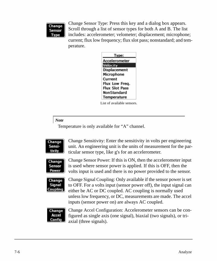
Change Sensor Type: Press this key and a dialog box appears. Scroll through a list of sensor types for both A and B. The list includes: accelerometer; velometer; displacement; microphone; current; flux low frequency; flux slot pass; nonstandard; and tem-perature.
List of available sensors.
NoteTemperature is only available for “A” channel.
Change Sensitivity: Enter the sensitivity in volts per engineering unit. An engineering unit is the units of measurement for the par-ticular sensor type, like g's for an accelerometer.
Change Sensor Power: If this is ON, then the accelerometer input is used where sensor power is applied. If this is OFF, then the volts input is used and there is no power provided to the sensor.
Change Signal Coupling: Only available if the sensor power is set to OFF. For a volts input (sensor power off), the input signal can either be AC or DC coupled. AC coupling is normally used unless low frequency, or DC, measurements are made. The accel inputs (sensor power on) are always AC coupled.
Change Accel Configuration: Accelerometer sensors can be con-figured as single axis (one signal), biaxial (two signals), or tri-axial (three signals).
7-6 Analyze
Set Overlap: Allows for faster data collection and is consistent with adequate data averaging. Data overlap controls the amount (%) that each new average overlaps the previous average when taking a measurement. This decreases the time required to collect data.
Overlapping data is a means of reusing a percentage of previously measured data to generate a new spectrum. The higher the overlap percentage, the less newly acquired data is needed to generate a spectrum, and thus faster the spectrum can be collected. This value ranges from 0% (no overlap) to 99%.The default overlap for the 2130 is 67%, and should be acceptable for most cases
Live Display Setup: Select the data that should be displayed during acquisi-tion. A dialog box appears when this key is pressed. Scroll through the list and select Status, Waveform, Spectrum, or the Dual option. This option is only used with Spectra and Third Octave acquisition modes.
Set Calib Factors: Press this key and go to a screen that allows you to modify the calibration factors listed below.
• Other channel: Allows you to toggle between channel A and channel B.• Edit Factors: Opens a screen so you can change the numbers for each calibra-
tion factor. Use the up/down arrow keys to scroll through the list. Press the enter key to return to the main Calibration Factors page.
• Show Current Factors: Displays current factors.• Show Default Factors: Returns the calibration factors back to factory default
settings.• Save Factors: Allows you to save your factors.
Caution!Changing calibration factors will affect data quality. Your ana-
lyzer is calibrated at the factory and should be re-calibrated annually.
Exits the Analyze program and returns you to the main screen.
7-7

Press Connect for Transfer to dump data to your computer for further analysis. Read more about this feature under “Connect for Transfer: Dumping Jobs” on page 7-62.
7-8 Analyze
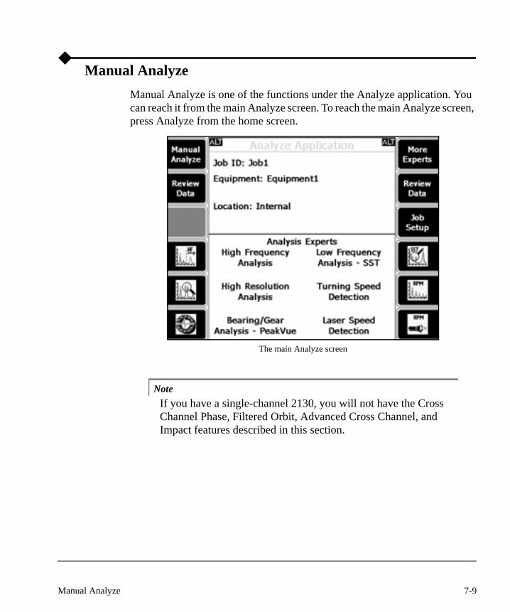
Manual AnalyzeManual Analyze is one of the functions under the Analyze application. You can reach it from the main Analyze screen. To reach the main Analyze screen, press Analyze from the home screen.
The main Analyze screen
NoteIf you have a single-channel 2130, you will not have the Cross Channel Phase, Filtered Orbit, Advanced Cross Channel, and Impact features described in this section.
7-9Manual Analyze

Press the Manual Analyze key on the main Analyze screen to open the Ana-lyze Setup menu.
The Manual Analyze screen
Press the Set Analyze Mode. A dialog box appears. Using the Arrow Up/Down keys you can scroll through a list of options until the one you want is highlighted. Press the Enter button to return to the Manual Analyze screen. Select the mode for the type of data you want to collect.
The list of available Analyze Modes.
7-10 Analyze
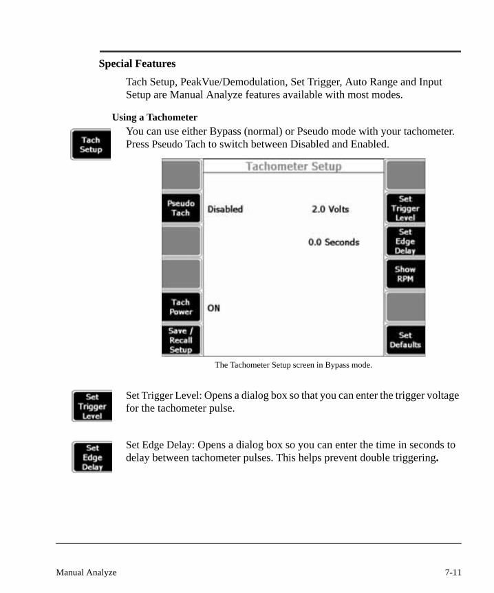
Special Features
Tach Setup, PeakVue/Demodulation, Set Trigger, Auto Range and Input Setup are Manual Analyze features available with most modes.
Using a TachometerYou can use either Bypass (normal) or Pseudo mode with your tachometer. Press Pseudo Tach to switch between Disabled and Enabled.
The Tachometer Setup screen in Bypass mode.
Set Trigger Level: Opens a dialog box so that you can enter the trigger voltage for the tachometer pulse.
Set Edge Delay: Opens a dialog box so you can enter the time in seconds to delay between tachometer pulses. This helps prevent double triggering.
7-11Manual Analyze

Show RPM: Press Show RPM to display the Last RPM and the Last Time.
1
Press Hide RPM to remove the RPM and Time features from your screen.
Tach Power: Toggle the tachometer’s power on and off.
Set Defaults: Returns you to the default tachometer settings for your analyzer.
Press Pseudo Tach to switch between Disabled and Enabled modes.
The Tachometer Setup screen in Pseudo mode.
Pseudo tach mode multiplies the incoming tach frequency by a ratio to gen-erate an output tach frequency to use during data acquisition. Use Pseudo mode when performing time synchronous averaging of gearboxes with inter-mediate shafts that cannot be accessed directly.
7-12 Analyze
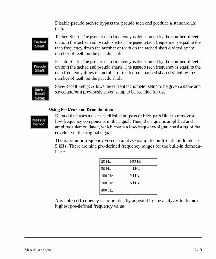
Disable pseudo tach to bypass the pseudo tach and produce a standard 1x tach.
Tached Shaft: The pseudo tach frequency is determined by the number of teeth on both the tached and pseudo shafts. The pseudo tach frequency is equal to the tach frequency times the number of teeth on the tached shaft divided by the number of teeth on the pseudo shaft.
Pseudo Shaft: The pseudo tach frequency is determined by the number of teeth on both the tached and pseudo shafts. The pseudo tach frequency is equal to the tach frequency times the number of teeth on the tached shaft divided by the number of teeth on the pseudo shaft.
Save/Recall Setup: Allows the current tachometer setup to be given a name and saved and/or a previously saved setup to be recalled for use.
Using PeakVue and DemodulationDemodulate uses a user-specified band-pass or high-pass filter to remove all low-frequency components in the signal. Then, the signal is amplified and amplitude demodulated, which create a low-frequency signal consisting of the envelope of the original signal.
The maximum frequency you can analyze using the built-in demodulator is 5 kHz. There are nine pre-defined frequency ranges for the built-in demodu-lator:
Any entered frequency is automatically adjusted by the analyzer to the next highest pre-defined frequency value.
20 Hz 500 Hz
50 Hz 1 kHz
100 Hz 2 kHz
200 Hz 5 kHz
400 Hz
7-13Manual Analyze
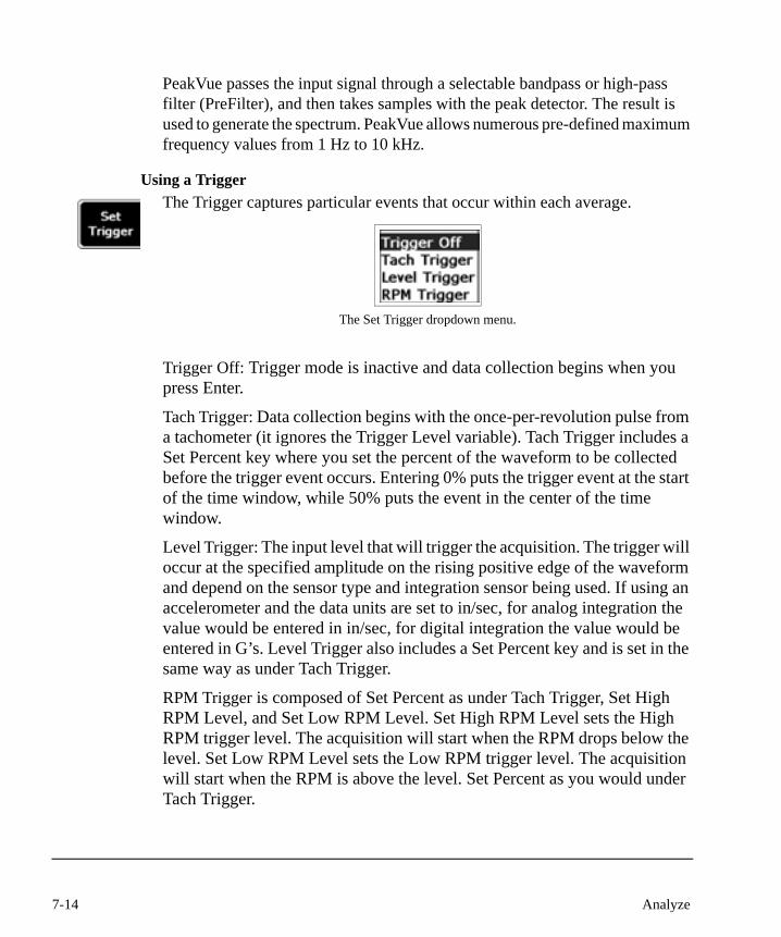
PeakVue passes the input signal through a selectable bandpass or high-pass filter (PreFilter), and then takes samples with the peak detector. The result is used to generate the spectrum. PeakVue allows numerous pre-defined maximum frequency values from 1 Hz to 10 kHz.
Using a TriggerThe Trigger captures particular events that occur within each average.
The Set Trigger dropdown menu.
Trigger Off: Trigger mode is inactive and data collection begins when you press Enter.
Tach Trigger: Data collection begins with the once-per-revolution pulse from a tachometer (it ignores the Trigger Level variable). Tach Trigger includes a Set Percent key where you set the percent of the waveform to be collected before the trigger event occurs. Entering 0% puts the trigger event at the start of the time window, while 50% puts the event in the center of the time window.
Level Trigger: The input level that will trigger the acquisition. The trigger will occur at the specified amplitude on the rising positive edge of the waveform and depend on the sensor type and integration sensor being used. If using an accelerometer and the data units are set to in/sec, for analog integration the value would be entered in in/sec, for digital integration the value would be entered in G’s. Level Trigger also includes a Set Percent key and is set in the same way as under Tach Trigger.
RPM Trigger is composed of Set Percent as under Tach Trigger, Set High RPM Level, and Set Low RPM Level. Set High RPM Level sets the High RPM trigger level. The acquisition will start when the RPM drops below the level. Set Low RPM Level sets the Low RPM trigger level. The acquisition will start when the RPM is above the level. Set Percent as you would under Tach Trigger.
7-14 Analyze
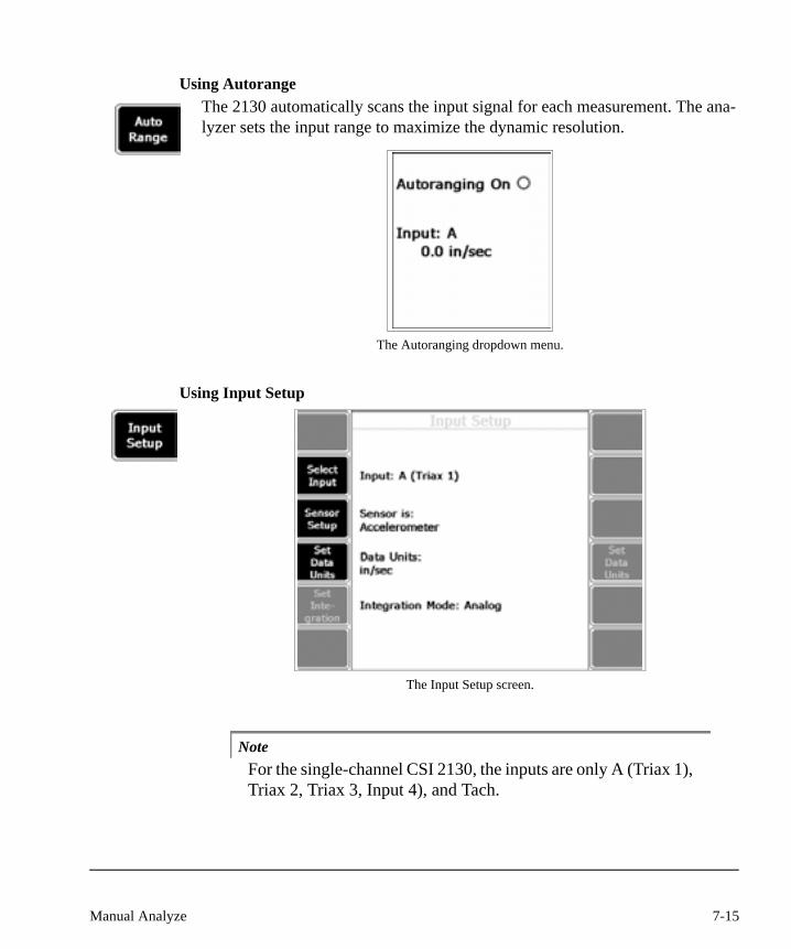
Using AutorangeThe 2130 automatically scans the input signal for each measurement. The ana-lyzer sets the input range to maximize the dynamic resolution.
The Autoranging dropdown menu.
Using Input Setup
The Input Setup screen.
NoteFor the single-channel CSI 2130, the inputs are only A (Triax 1), Triax 2, Triax 3, Input 4), and Tach.
7-15Manual Analyze
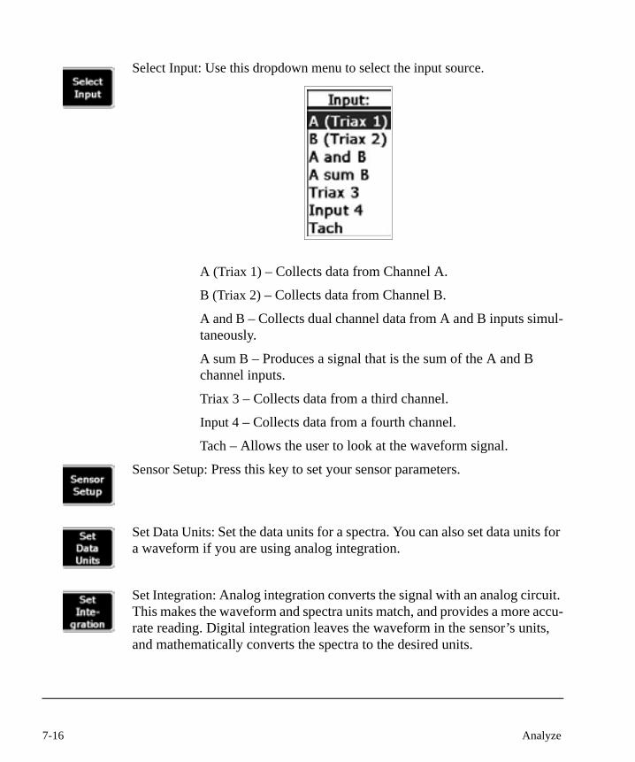
Select Input: Use this dropdown menu to select the input source.
2
A (Triax 1) – Collects data from Channel A.
B (Triax 2) – Collects data from Channel B.
A and B – Collects dual channel data from A and B inputs simul-taneously.
A sum B – Produces a signal that is the sum of the A and B channel inputs.
Triax 3 – Collects data from a third channel.
Input 4 – Collects data from a fourth channel.
Tach – Allows the user to look at the waveform signal.
Sensor Setup: Press this key to set your sensor parameters.
Set Data Units: Set the data units for a spectra. You can also set data units for a waveform if you are using analog integration.
Set Integration: Analog integration converts the signal with an analog circuit. This makes the waveform and spectra units match, and provides a more accu-rate reading. Digital integration leaves the waveform in the sensor’s units, and mathematically converts the spectra to the desired units.
7-16 Analyze

Spectra
The vibration spectrum is the basic tool for understanding the nature of the vibration. To create a spectrum that is as informative as possible, you must set the measurement parameters appropriately.
A vibration spectrum is a graph of vibration amplitude versus vibration fre-quency. The vibration spectrum of a machine component shows the frequen-cies at which the component is vibrating and the amplitude of vibration at each of these frequencies.Setting Spectrum Parameters
The Analyze Setup screen in Spectra mode.
NoteSpectra is the most commonly used Analyze mode.
7-17Manual Analyze

Set Spectra Params: Allows you to set spectra parameters. Brings you to a second screen of options:
The Spectra Parameters dropdown menu.
Set FMAX: Set the maximum frequency for your spectrum. The Fmax is the maximum frequency displayed on the spectrum. Or more specifically the fre-quency range, starting from zero, over which vibration amplitudes are dis-played.
In general, the higher the operating speed of a machine, the higher the fmax needs to be to capture all crucial information. For vibration involving fin-gered elements such as gear teeth, fan blades, pump vanes and bearing ele-ments, an fmax equal to 3 times the number of fingers multiplied by the operating speed is usually sufficient. For vibration not involving fingered ele-ments, an fmax equal to 10 times the operating speed is usually sufficient.
A setting of 200-400 Hz (12000-24000 cpm) is sufficient for most coast up, coast down recordings.
Set Low Cutoff: Use the number keys to enter a new number. Left and right arrows move the cursor. The Alt Delete Digit key deletes the digit to the left of the cursor. The Alt Clear number key clears the entire number. The Go-Back key reloads the original number.
The low cutoff removes very low frequency integration noise from the overall measurement and is normally set at 2 Hz.
7-18 Analyze

Set Lines: The resolution of the spectrum increases with the number of spectral lines used. This means the more spectral lines, the more information the spec-trum contains. However, if more spectral lines are used, it takes longer to mea-sure and more memory is used to store the spectrum. You may want to reserve high resolution measurements for applications such as when you need to dis-tinguish between two closely spaced vibration frequencies or when the fmax is very large. For coast-up, coast-down recordings, a setting of 400 is recom-mended.
For synchronous time, order tracking, and cross channel acquisitions the number of lines is limited to 1600. For dual channel acquisitions, the number of lines is limited to 6400. Use the up and down arrow keys to select a value. Enter accepts the value. Back reloads the original value.
2130 spectra consist of discrete spectral lines that are displayed at fixed fre-quency intervals. The height of each spectral line represents the amplitude of vibration at the frequency the spectral line is positioned.
NoteThe 2130 can have a maximum resolution of 12,800 lines for single channel data.
NoteYou can measure velocity in most situations. However, for low frequencies (below 1800 cpm), displacement spectra are more informative. For high frequencies (above 60k cpm), acceleration spectra are more informative.
Set Window: Waveform data is processed by FFT (Fast Fourier Transform) to create a spectral plot. To prevent the spectral lines from bleeding into each other, the data is usually multiplied by a Hanning window function.
NoteUse the Hanning window in most situations. A Uniform window is only used in certain transient applications where the entire signal is contained inside a single time block.
7-19Manual Analyze
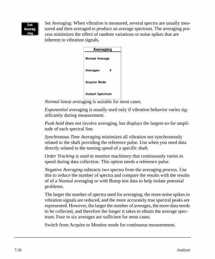
Set Averaging: When vibration is measured, several spectra are usually mea-sured and then averaged to produce an average spectrum. The averaging pro-cess minimizes the effect of random variations or noise spikes that are inherent to vibration signals.
Normal linear averaging is suitable for most cases.
Exponential averaging is usually used only if vibration behavior varies sig-nificantly during measurement.
Peak hold does not involve averaging, but displays the largest-so-far ampli-tude of each spectral line.
Synchronous Time Averaging minimizes all vibration not synchronously related to the shaft providing the reference pulse. Use when you need data directly related to the turning speed of a specific shaft.
Order Tracking is used to monitor machinery that continuously varies in speed during data collection. This option needs a reference pulse.
Negative Averaging subtracts two spectra from the averaging process. Use this to reduce the number of spectra and compare the results with the results of of a Normal averaging or with Bump test data to help isolate potential problems.
The larger the number of spectra used for averaging, the more noise spikes in vibration signals are reduced, and the more accurately true spectral peaks are represented. However, the larger the number of averages, the more data needs to be collected, and therefore the longer it takes to obtain the average spec-trum. Four to six averages are sufficient for most cases.
Switch from Acquire to Monitor mode for continuous measurement.
7-20 Analyze
Switch between Instant Spectra and Average spectrum to view either the last measurement or the average of all the measurements during data collection.
Set SST/Aweighting: Select Aweighting to apply a shape curve to the acquired frequency spectrum that approximates the frequency sensitivity of the human ear. A-weighting is used with microphone signals, and is used when you want to see perceived “loudness.”
SST (slow speed technology) lets the analyzer make accurate, low-frequency measurements when integrating to velocity or displacement. Normally, low frequency peaks are difficult to see when an accelerometer is used, and the peaks are converted to velocity or displacement. SST employs a special cor-rection technique to correct the non-linear response of the integrators and lets you accurately measure peaks as low as 10 RPM.
A high-sensitivity, low-frequency sensor is best for measurements as low as 10 RPM. Use general purpose accelerometer, such as Part No. A0760GP, for measurements as low as 40 RPM. Contact customer support for recommen-dations if you plan to measure lower frequencies.
7-21Manual Analyze

Waveform
A vibration waveform is a graph that shows how vibration level changes with time. The waveform shows the vibration level at any particular instant during the measurement period.
The analyzer’s waveforms are discrete graphs represented by a series of equally-spaced, discrete sample points (connected by straight lines). The more sample points in a spectrum, the higher the resolution of the waveform (but the more memory used).
To ensure a waveform is as informative as possible, you must set the mea-surement parameters appropriately.
Setting the Analyze mode to waveform monitors a continuous stream of time waveform data.
Setting Waveform Parameters
The Analyze Setup screen in Waveform mode.
Set FMAX: Set the maximum frequency for your waveform. The Fmax is the maximum frequency displayed on the waveform. Or more specifically the frequency range, starting from zero, over which vibration amplitudes are displayed.
7-22 Analyze
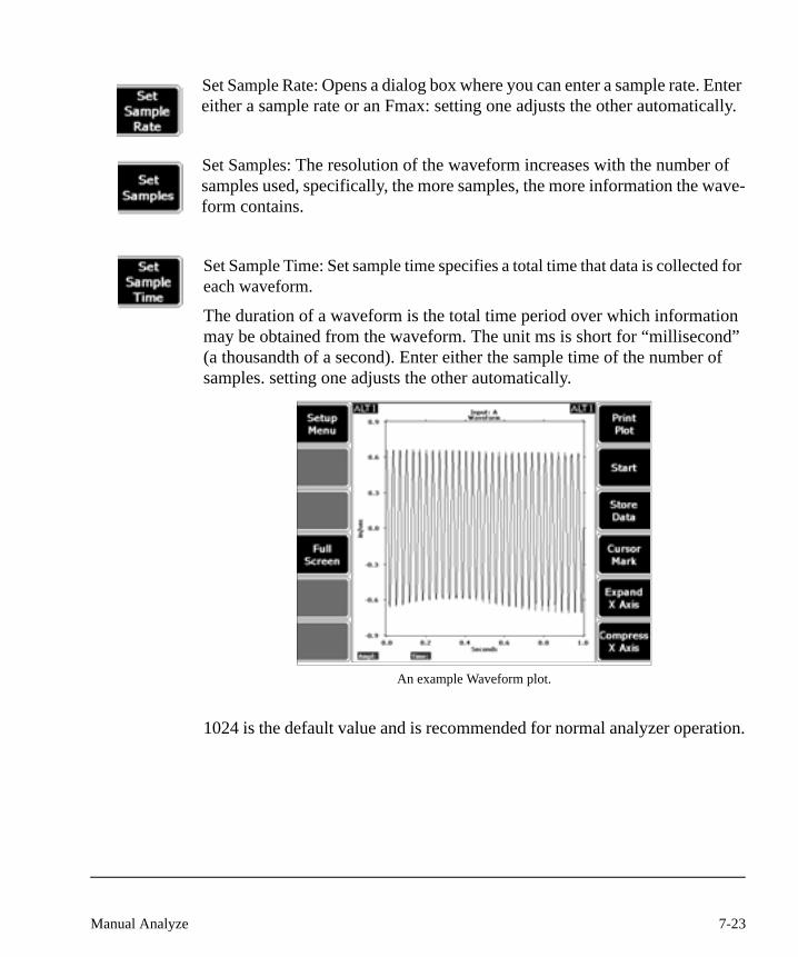
Set Sample Rate: Opens a dialog box where you can enter a sample rate. Enter either a sample rate or an Fmax: setting one adjusts the other automatically.
Set Samples: The resolution of the waveform increases with the number of samples used, specifically, the more samples, the more information the wave-form contains.
Set Sample Time: Set sample time specifies a total time that data is collected for each waveform.
The duration of a waveform is the total time period over which information may be obtained from the waveform. The unit ms is short for “millisecond” (a thousandth of a second). Enter either the sample time of the number of samples. setting one adjusts the other automatically.
An example Waveform plot.
1024 is the default value and is recommended for normal analyzer operation.
7-23Manual Analyze

Overall
Setting the Analyze mode to Overall allows you to watch a piece of machinery over longer times in order to monitor changes.
Setting Overall Parameters
The Analyze Setup screen in Overall mode.
Set Overall Mode: Set your Overall acquisition to Broadband or Frequency Band. Broadband mode acquires broadband waveform data, and calculates the overall as the RMS value of the waveform. The range of frequencies included in the overall value is 1 Hz to 80kHz.
Frequency Band mode calculates the overall value from a normal spectral acquisition and includes frequencies between the Fhigh and Flow values.
Set Spectra Params: When using the Frequency Band mode, specify the upper and lower frequency limit, the number of averages, etc.
Set Time Increments: When using Broadband mode, set the minimum wait time between each measurement.
7-24 Analyze

Set Number of Points: Determines the number of points that are collected during acquisition.
Set Collection Mode: Overall acquisition can be continuous or non-contin-uous. Continuous mode collects the required number of points and continues collecting data, replacing the oldest data with new data.
Non-continuous mode only collects the required number of points and then stops collecting data.
Set Alarm Level: Establish an alarm level for the measurement. If the mea-surement exceeds the specified alarm level, the analyzer gives a warning beep. The warning beeps continue until the acquisition stops or the signal drops back below the alarm level. Enter zero (0) to disable the alarm feature.
NoteFor dual overall acquisitions, the user can set an alarm for both A and B inputs.
Set Time Span: Determines the displayed time span of the trend plot.
DC Volts and Temperature
The analyze modes of DC Volts and Temperature measurements are similar to Overall measurements. The analyzer trends over time in order to produce a strip plot.
7-25Manual Analyze
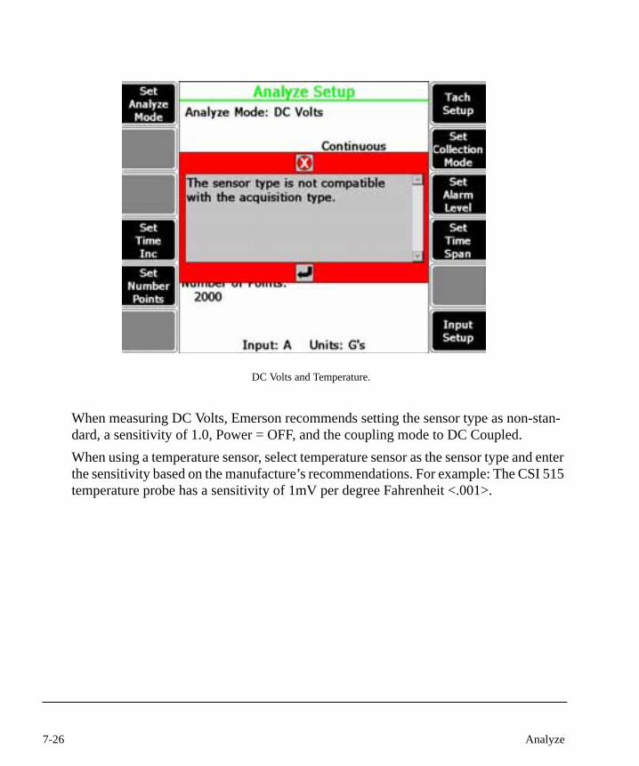
DC Volts and Temperature.
When measuring DC Volts, Emerson recommends setting the sensor type as non-stan-dard, a sensitivity of 1.0, Power = OFF, and the coupling mode to DC Coupled.When using a temperature sensor, select temperature sensor as the sensor type and enter the sensitivity based on the manufacture’s recommendations. For example: The CSI 515 temperature probe has a sensitivity of 1mV per degree Fahrenheit <.001>.
7-26 Analyze
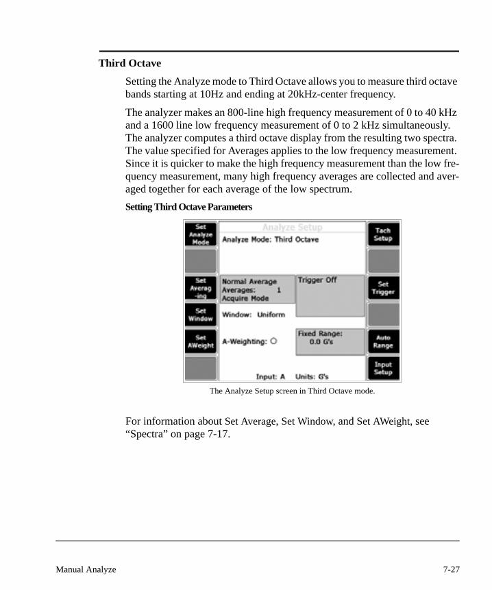
Third Octave
Setting the Analyze mode to Third Octave allows you to measure third octave bands starting at 10Hz and ending at 20kHz-center frequency.
The analyzer makes an 800-line high frequency measurement of 0 to 40 kHz and a 1600 line low frequency measurement of 0 to 2 kHz simultaneously. The analyzer computes a third octave display from the resulting two spectra. The value specified for Averages applies to the low frequency measurement. Since it is quicker to make the high frequency measurement than the low fre-quency measurement, many high frequency averages are collected and aver-aged together for each average of the low spectrum.Setting Third Octave Parameters
The Analyze Setup screen in Third Octave mode.
For information about Set Average, Set Window, and Set AWeight, see “Spectra” on page 7-17.
7-27Manual Analyze

For information about Tach Setup, Set Trigger, Auto Range and Input Setup, see “Special Features” on page 7-11.
An example Third Octave plot.
7-28 Analyze
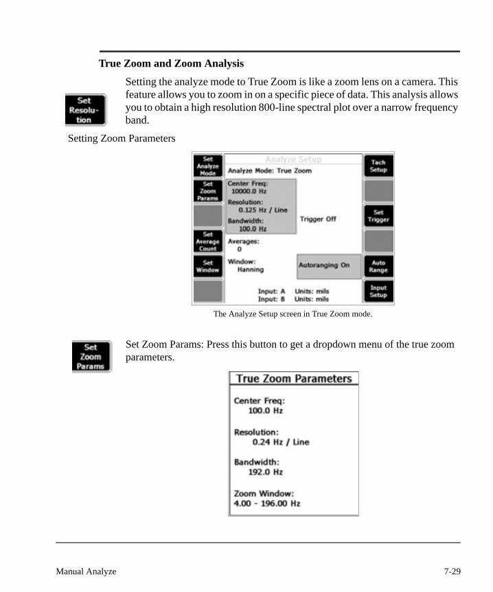
True Zoom and Zoom Analysis
Setting the analyze mode to True Zoom is like a zoom lens on a camera. This feature allows you to zoom in on a specific piece of data. This analysis allows you to obtain a high resolution 800-line spectral plot over a narrow frequency band.
Setting Zoom Parameters
The Analyze Setup screen in True Zoom mode.
Set Zoom Params: Press this button to get a dropdown menu of the true zoom parameters.
3
7-29Manual Analyze

Set Center Frequency: This is the frequency of interest.
Set Resolution: Enter the resolution in Hz or CPM (see more information about resolution on page 8-7).
Set Bandwidth: Set the bandwidth of the zoom frequency window.
NoteThe resolution and bandwidth fields work together. Changing one changes both settings.
Set Average Count: Enter the number of averages you want to use to compile your plot.
7-30 Analyze
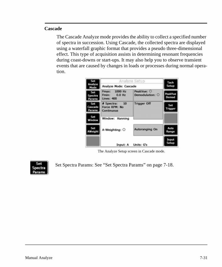
Cascade
The Cascade Analyze mode provides the ability to collect a specified number of spectra in succession. Using Cascade, the collected spectra are displayed using a waterfall graphic format that provides a pseudo three-dimensional effect. This type of acquisition assists in determining resonant frequencies during coast-downs or start-ups. It may also help you to observe transient events that are caused by changes in loads or processes during normal opera-tion.
The Analyze Setup screen in Cascade mode.
Set Spectra Params: See “Set Spectra Params” on page 7-18.
7-31Manual Analyze
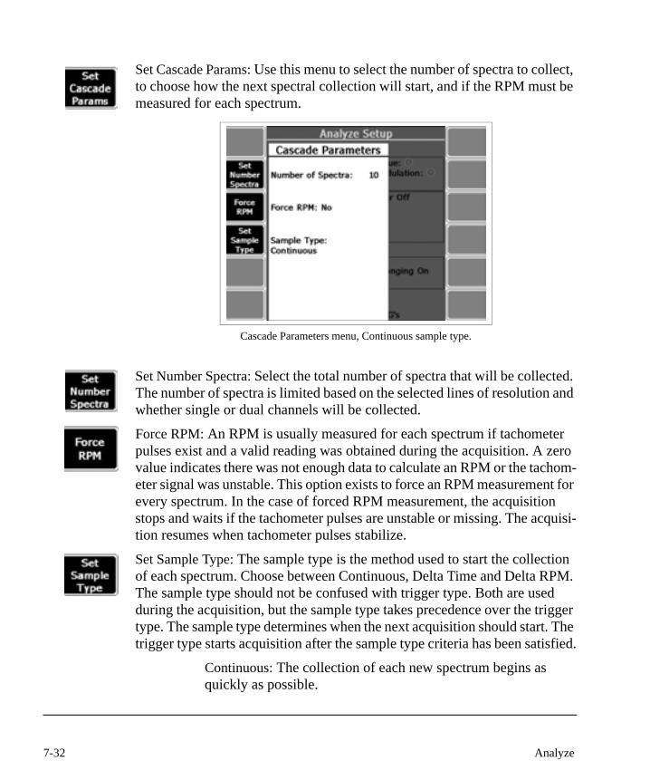
Set Cascade Params: Use this menu to select the number of spectra to collect, to choose how the next spectral collection will start, and if the RPM must be measured for each spectrum.
Cascade Parameters menu, Continuous sample type.
Set Number Spectra: Select the total number of spectra that will be collected. The number of spectra is limited based on the selected lines of resolution and whether single or dual channels will be collected.
Force RPM: An RPM is usually measured for each spectrum if tachometer pulses exist and a valid reading was obtained during the acquisition. A zero value indicates there was not enough data to calculate an RPM or the tachom-eter signal was unstable. This option exists to force an RPM measurement for every spectrum. In the case of forced RPM measurement, the acquisition stops and waits if the tachometer pulses are unstable or missing. The acquisi-tion resumes when tachometer pulses stabilize.
Set Sample Type: The sample type is the method used to start the collection of each spectrum. Choose between Continuous, Delta Time and Delta RPM. The sample type should not be confused with trigger type. Both are used during the acquisition, but the sample type takes precedence over the trigger type. The sample type determines when the next acquisition should start. The trigger type starts acquisition after the sample type criteria has been satisfied.
Continuous: The collection of each new spectrum begins as quickly as possible.
7-32 Analyze

Delta Time: The collection of each new spectrum begins after a specified time interval has elapsed, since the start of the previous spectrum.
Delta RPM: The collection of each new spectrum begins after a specified change in RPM.
Cascade Parameters menu, Delta Time sample type.
Set Time Delay: When using the Delta Time sample type, select the minimum time delay (in seconds), between the start of each collected spectrum. The delay period is measured from the start of the current acquisition to the start of the next.
7-33Manual Analyze

A minimum delay exists because of the processing time that is required for data acquisition. If non-zero values that are less than the minimum required are entered, they are increased to the minimum value automatically. If you enter zero, the spectra is collected as quickly as possible, without delay.
Cascade Parameters menu, Delta RPM sample type.
Set RPM Mode: When the Delta RPM sample type is selected, a change in RPM must be detected between each spectral collection. The RPM change can be detected in one of three ways:
+RPM: Increasing changes in RPM are detected.
-RPM: Decreasing changes in RPM are detected.
+/-RPM: Both increasing and decreasing changes in RPM are detected.
Set Delta RPM: When using Delta RPM sample type, select the minimum value of RPM change required between consecutive data collections.
Set Window: See “Set Window” on page 7-19.
7-34 Analyze

Set AWeight: Toggles A-weighting on and off. Select A-weighting to apply a shape curve to the acquired frequency spectrum that approximates the fre-quency sensitivity of the human ear. A-weighting is used with microphone signals, and is used when you want to see perceived “loudness.”
Tach Setup: See “Using a Tachometer” on page 7-11.
PeakVue/Demod: See “Using PeakVue and Demodulation” on page 7-13.
Set Trigger: This key enables the Tach Trigger, Level Trigger, or RPM Trigger modes to start Cascade acquisitions when the trigger level is reached. These trigger types are available in other acquisitions, see “Using a Trigger” on page 7-14 for more information.
Some notable differences exist when a trigger is used with a cascade acquisi-tion. The Level Trigger and RPM Trigger are only used to start collection of the very first spectrum in the series. All other spectra are collected without a trigger. Also, these two modes do not permit pre-triggering. When using the Tach Trigger with Cascade, a Set Tach Start option is available.
Tachometer Trigger Setup menu.
7-35Manual Analyze

Set Tach Start: This is only available when Tach Trigger is selected. It speci-fies how the trigger will be applied during the collection of a series of spectra.
All: A tachometer pulse triggers the start of each spectral collec-tion. In this mode, pre-triggering is permitted.
First: A tachometer pulse triggers the very first spectrum that is collected. All subsequent spectra is collected without using the tachometer pulse as a trigger. Pre-triggering is not permitted in this mode.
Autorange: See “Using Autorange” on page 7-15.
Input Setup: See “Input Setup” on page 8-15.
7-36 Analyze
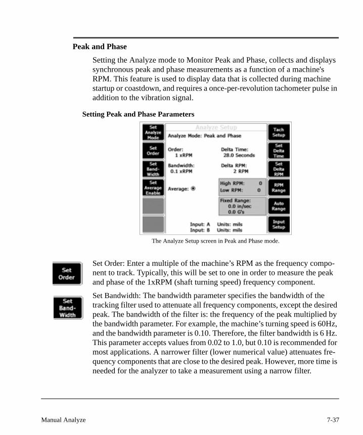
Peak and Phase
Setting the Analyze mode to Monitor Peak and Phase, collects and displays synchronous peak and phase measurements as a function of a machine's RPM. This feature is used to display data that is collected during machine startup or coastdown, and requires a once-per-revolution tachometer pulse in addition to the vibration signal.
Setting Peak and Phase Parameters
The Analyze Setup screen in Peak and Phase mode.
Set Order: Enter a multiple of the machine’s RPM as the frequency compo-nent to track. Typically, this will be set to one in order to measure the peak and phase of the 1xRPM (shaft turning speed) frequency component.
Set Bandwidth: The bandwidth parameter specifies the bandwidth of the tracking filter used to attenuate all frequency components, except the desired peak. The bandwidth of the filter is: the frequency of the peak multiplied by the bandwidth parameter. For example, the machine’s turning speed is 60Hz, and the bandwidth parameter is 0.10. Therefore, the filter bandwidth is 6 Hz. This parameter accepts values from 0.02 to 1.0, but 0.10 is recommended for most applications. A narrower filter (lower numerical value) attenuates fre-quency components that are close to the desired peak. However, more time is needed for the analyzer to take a measurement using a narrow filter.
7-37Manual Analyze

Set Average Enable: Select this function to vector average each new measure-ment with the previous measurement. This feature is useful when monitoring a running machine if the peak or phase readings fluctuate from measurement to measurement, or if the frequency of interest is modulated by nearby fre-quency components.
NoteThis option should not be enabled when doing a startup or coast-down data collection.
Set Delta Time: This is the time in seconds that elapse between data points that are being stored. If set to zero, a data point is stored whenever the RPM changes by the Delta RPM (or by 1% if not specified).
Set Delta RPM: This is the change in the RPM that must occur before a data point is stored. Set to zero to store a data point whenever the RPM changes by 1%.
RPM Range: These are the minimum and maximum RPM values. If the mea-sured RPM is less than the minimum value or greater than the maximum value, no data collection or analysis is performed. The message “RPM out of Range” displays. Enter zero (0) to disable this feature.
7-38 Analyze
Filtered Orbit
Setting the Analyze mode to Filtered Orbit is useful for analyzing the phase relationship between two channels at a specific order of turning speed. Orbit plots usually indicate the trace of the relative movement of a rotating shaft with respect to some reference point. The 2130 can create an orbit plot using the waveform data from any dual measurement point pair.
Time waveform data is normally plotted as amplitude (vertical) versus time (horizontal). The same waveform data can be used to generate an orbit plot by plotting channel A amplitude (horizontal) vs. channel B amplitude (ver-tical) from a pair of shaft displacement probes. The resulting display pattern represents the movement of the shaft.
Orbit plots can be generated using normal dual channel route based data, but this requires the user to set up the acquisition to collect the correct amount of data to generate a good orbit plot and it does not provide filtering. Using the Filtered Orbit feature in the Analyze program eliminates the complicated setup. Filtering the data provides added benefits:
You can arrange the orbit’s parameters so that only the frequencies you are interested in are included in the orbit plot.
The orbit plot is less complicated, so the pattern is easier to recognize.
Setting Orbit ParametersOrbit Mode: Toggle between the Bandpass and Lowpass Filtered Orbit modes.
7-39Manual Analyze

The Analyze Setup Screen in Bandpass Orbit mode.
Band Pass Filter: The analyzer calculates peak and phase data for both channels using a tachometer input. It then creates two wave-forms from the peak and phase data and plots these values in the X (horizontal) and Y (vertical) directions. The orbit plot is then a representation of a band pass filtered signal.
The Analyze Setup Screen in Lowpass Orbit mode.
7-40 Analyze
Low Pass Filter: Use this mode with or without a tachometer, and it includes all frequencies at and below RPM times orders. In the Low Pass mode the analyzer does low pass filtering on the data as it is collected. All frequencies above the “orders times RPM” value are filtered out when the waveforms are collected. The actual collected waveform data are plotted in the orbit. Since this method creates a plot that includes all frequencies from the desired order level and lower, it will show more complex orbits that can indicate rubs, misalignment, or oil whip.
Set Order: The Orbit Orders parameter selects between 1X, 2X, or 3X the shaft turning speed.
Set Number of Revolutions: This is the number of revolutions to display in the orbit plot. This can be a whole number from one through nine.
Use Tach: If a tachometer is not used, then the filter is set based on manual RPM entry. If a tachometer is used, the filter is constantly updated for changing machine speeds and the orbit will be phase related to the sensor.
NoteFiltered Orbit is only available for the dual-channel CSI 2130.
7-41Manual Analyze

Cross Channel Phase
Setting the Analyze mode to cross channel phase uses cross-channel spectra to calculate phase and coherence relationships between the two channels. You can set the mode to monitor a single frequency or to acquire full spectral plots.Setting Cross Channel Phase Parameters
The Analyze Setup screen in Cross Channel Phase mode.
Set Mode: The Single Frequency Monitor function calculates the cross power phase relationship between channels A and B at a specified frequency, and calculates a coherence value for this relationship.
In Full Spectrum mode, Dual channel spectral data is collected with a speci-fied number of averages and plots the phase, coherence, as well as the spectral data for each channel.
NoteCross Channel data cannot be stored.
7-42 Analyze

Set Frequency: The Frequency variable is used to specify the phase frequency for which the cross channel phase and coherence are calculated.
NoteThe Set Freq key is only seen from the Single Frequency mode.
NoteThe cross channel phase is only available on the dual-channel CSI 2130.
7-43Manual Analyze
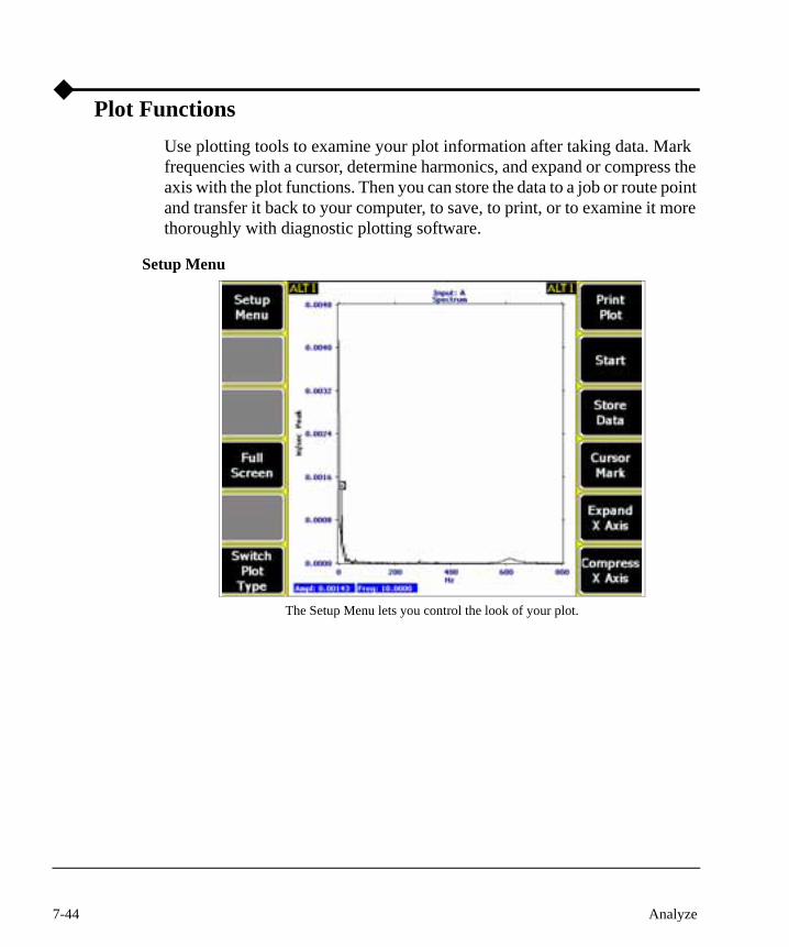
Plot FunctionsUse plotting tools to examine your plot information after taking data. Mark frequencies with a cursor, determine harmonics, and expand or compress the axis with the plot functions. Then you can store the data to a job or route point and transfer it back to your computer, to save, to print, or to examine it more thoroughly with diagnostic plotting software.
Setup Menu
The Setup Menu lets you control the look of your plot.
7-44 Analyze
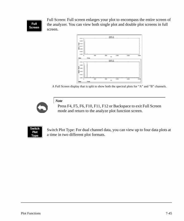
Full Screen: Full screen enlarges your plot to encompass the entire screen of the analyzer. You can view both single plot and double plot screens in full screen.
A Full Screen display that is split to show both the spectral plots for “A” and “B” channels.
NotePress F4, F5, F6, F10, F11, F12 or Backspace to exit Full Screen mode and return to the analyze plot function screen.
Switch Plot Type: For dual channel data, you can view up to four data plots at a time in two different plot formats.
7-45Plot Functions

You can view up to four plots at one time.
This is the “stacked” plot view.
7-46 Analyze
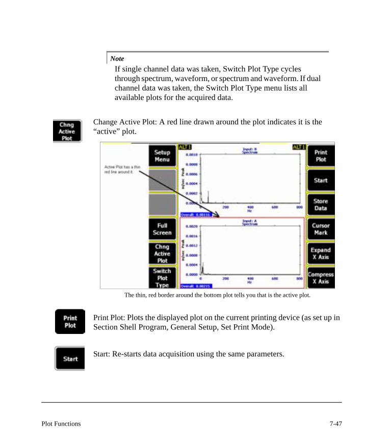
NoteIf single channel data was taken, Switch Plot Type cycles through spectrum, waveform, or spectrum and waveform. If dual channel data was taken, the Switch Plot Type menu lists all available plots for the acquired data.
Change Active Plot: A red line drawn around the plot indicates it is the “active” plot.
The thin, red border around the bottom plot tells you that is the active plot.
Print Plot: Plots the displayed plot on the current printing device (as set up in Section Shell Program, General Setup, Set Print Mode).
Start: Re-starts data acquisition using the same parameters.
7-47Plot Functions

Store Data: Stores your data to a route or job.
Current Job screen
Cursor Mark: The cursor mark provides a more accurate indication of the cursor’s location. This may be used to determine the exact frequency and amplitude of a peak. Place the cursor on top of any peak and press cursor mark to update the values. This key is also used to mark a frequency of interest for the analysis expert.
Expand X: Expands a section of the X axis. The total span of the x axis is cut in half. If a cursor is active, the new scale tries to center on the cursor position. If no cursor is active, the new scale expands the center section of the plot.
Compress X: Compresses the displayed area of the x axis. the total span of the x axis doubles. If a cursor is active the new scales tries to center on the cursor’s position. If no cursor is active, the new scale contracts around the center section of the plot.
7-48 Analyze

ALT screen keysBelow is a list of keys you will find by pressing the analyzer’s ALT button. A few of the keys are repeated from the first screen to the ALT screen.
4
Set RPM: The Set RPM only works if additional Analyze data is collected from a route point setup, the RPM marked will now become the new speed for the next route point to be collected. The Order selection is only available if Analyze data is collected from a route point setup. After the RPM has been set, pressing the X-Axis Units will toggle from Hz, CPM, and Orders.
Cursor Type: Press this key once to see the current cursor type. A green box will pop up in the middle of the screen listing the current cursor type. Quickly press it again to change the cursor type. Keep pressing until you see the cursor type you want. The six cursor types available are: normal, harmonic, moving harmonic, sideband cursors for spectrum plots, Harmonic Family, and Har-monic Difference.
7-49Plot Functions
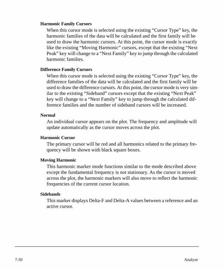
Harmonic Family CursorsWhen this cursor mode is selected using the existing “Cursor Type” key, the harmonic families of the data will be calculated and the first family will be used to draw the harmonic cursors. At this point, the cursor mode is exactly like the existing “Moving Harmonic” cursors, except that the existing “Next Peak” key will change to a “Next Family” key to jump through the calculated harmonic families.
Difference Family CursorsWhen this cursor mode is selected using the existing “Cursor Type” key, the difference families of the data will be calculated and the first family will be used to draw the difference cursors. At this point, the cursor mode is very sim-ilar to the existing “Sideband” cursors except that the existing “Next Peak” key will change to a “Next Family” key to jump through the calculated dif-ference families and the number of sideband cursors will be increased.
NormalAn individual cursor appears on the plot. The frequency and amplitude will update automatically as the cursor moves across the plot.
Harmonic CursorThe primary cursor will be red and all harmonics related to the primary fre-quency will be shown with black square boxes.
Moving HarmonicThis harmonic marker mode functions similar to the mode described above except the fundamental frequency is not stationary. As the cursor is moved across the plot, the harmonic markers will also move to reflect the harmonic frequencies of the current cursor location.
SidebandsThis marker displays Delta-F and Delta-A values between a reference and an active cursor.
7-50 Analyze
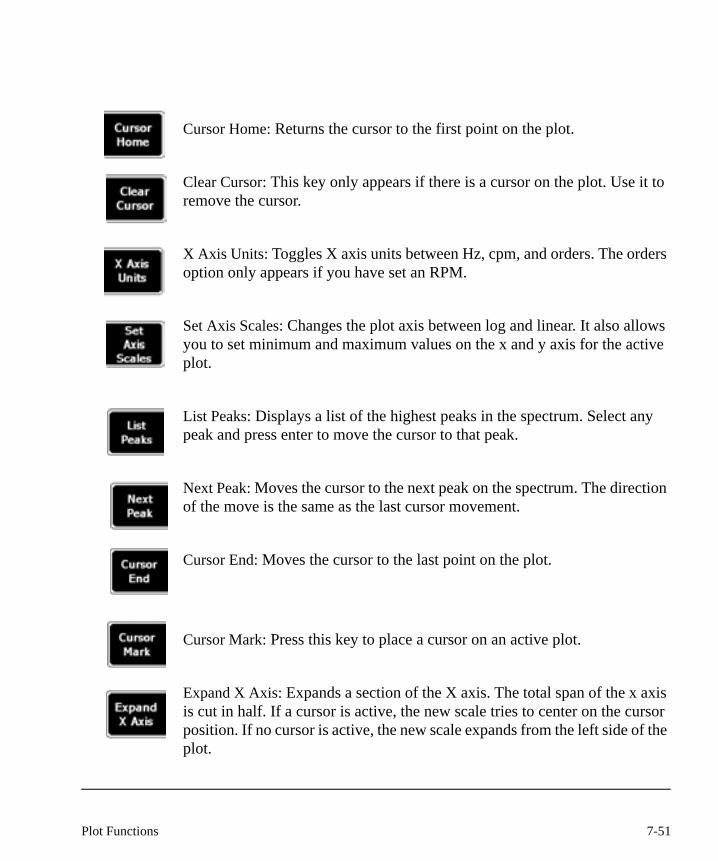
Cursor Home: Returns the cursor to the first point on the plot.
Clear Cursor: This key only appears if there is a cursor on the plot. Use it to remove the cursor.
X Axis Units: Toggles X axis units between Hz, cpm, and orders. The orders option only appears if you have set an RPM.
Set Axis Scales: Changes the plot axis between log and linear. It also allows you to set minimum and maximum values on the x and y axis for the active plot.
List Peaks: Displays a list of the highest peaks in the spectrum. Select any peak and press enter to move the cursor to that peak.
Next Peak: Moves the cursor to the next peak on the spectrum. The direction of the move is the same as the last cursor movement.
Cursor End: Moves the cursor to the last point on the plot.
Cursor Mark: Press this key to place a cursor on an active plot.
Expand X Axis: Expands a section of the X axis. The total span of the x axis is cut in half. If a cursor is active, the new scale tries to center on the cursor position. If no cursor is active, the new scale expands from the left side of the plot.
7-51Plot Functions

Compress X Axis: Compresses the displayed area of the x axis. the total span of the x axis doubles. If a cursor is active the new scales tries to center on the cursor’s position. If no cursor is active, the new scale contracts to the left.
7-52 Analyze
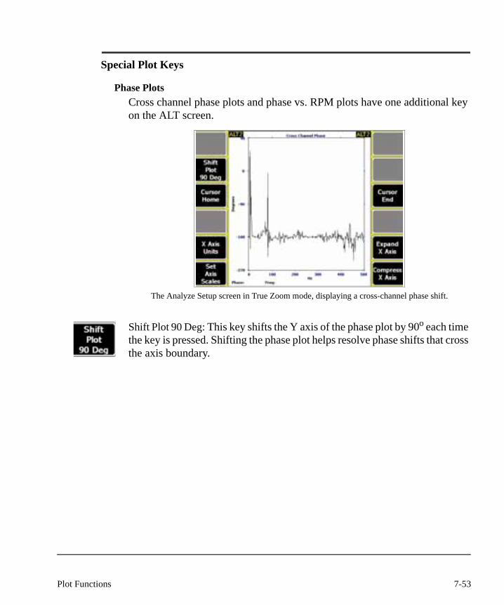
Special Plot Keys
Phase PlotsCross channel phase plots and phase vs. RPM plots have one additional key on the ALT screen.
The Analyze Setup screen in True Zoom mode, displaying a cross-channel phase shift.
Shift Plot 90 Deg: This key shifts the Y axis of the phase plot by 90o each time the key is pressed. Shifting the phase plot helps resolve phase shifts that cross the axis boundary.
7-53Plot Functions
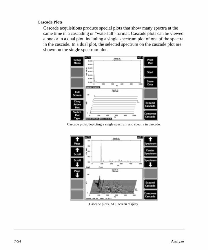
Cascade PlotsCascade acquisitions produce special plots that show many spectra at the same time in a cascading or “waterfall” format. Cascade plots can be viewed alone or in a dual plot, including a single spectrum plot of one of the spectra in the cascade. In a dual plot, the selected spectrum on the cascade plot are shown on the single spectrum plot.
Cascade plots, depicting a single spectrum and spectra in cascade.
Cascade plots, ALT screen display.
7-54 Analyze

Cascade plots may be compressed automatically by the analyzer if there are more spectra in the cascade than can fit on the plot. In this case, some inter-mediate spectra may be “skipped” or removed from the plot so that an over-view of the entire cascade can be viewed.
Expanding the cascade plot reduces the number of skipped spectra, but it also reduces the total range of spectra shown. This results in the plot leaving off spectra at the beginning or the end of the plot, and a section of total cascade data is displayed. The displayed section of the total cascade can be changed using the Page or Scroll keys.
A red arrow on the right side of the cascade plot indicates the current selected spectrum. The time relative to the start of the cascade and the speed measured when the selected spectrum was collected is shown at the bottom of the plot. If a single spectrum plot for the cascade is active then the selected spectrum is shown on that plot. The single spectrum plot changes if the selected plot in the cascade is changed.
Expand Cascade: Reduces the size of the cascade section. The number of skipped spectra reduces until none are skipped, and then the individual spectra are moved further apart.
Compress Cascade: Increases the size of the cascade section. The individual spectra move closer together and then the number of skipped spectra increases.
Page Up/Page Down: Move the section of the cascade that is shown by one of the number of spectra that is currently on the plot.
Scroll Up/Scroll Down: Move the section of the cascade shown by 1/4 of the number of spectra currently on the plot.
Spectrum Up/Spectrum Down: Change the currently marked spectrum.
Center Spectrum: Tries to center the cascade plot on the currently selected spectrum. The plot may not center completely if the selected plot is near the beginning or end of the cascade.
7-55Plot Functions

Auto Correlation
Waveform plots have an additional key on the ALT screen. The Enhance Pat-terns key is used to calculate the Auto Correlation waveform plot from the active waveform plot. The Auto Correlation function is a way to determine if there is a repetitive pattern within a time waveform.
Auto Correlation waveform plot
Enhance Patterns: When the active plot is a waveform plot that does not have an Auto Correlation plot calculated, this key is active and set to Enhance Pat-terns. When this key is active, it can be used to replace the active waveform plot (and only the active waveform plot, if data from a dual channel acquisi-tion is displayed) with an Auto Correlation plot. When the active plot is a waveform plot has an Auto Correlation plot calculated, this key is not used. In the Analyze program, this key is not available when acquiring data in the monitor mode.
7-56 Analyze
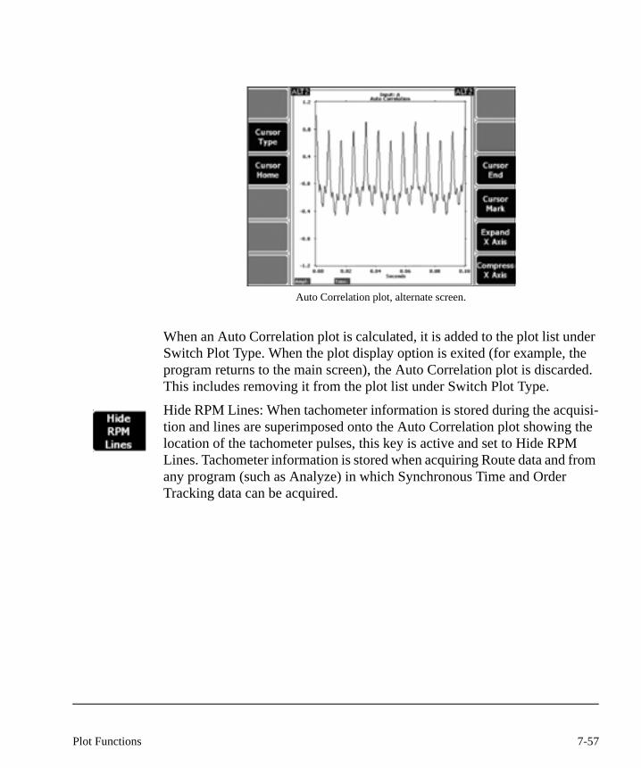
Auto Correlation plot, alternate screen.
When an Auto Correlation plot is calculated, it is added to the plot list under Switch Plot Type. When the plot display option is exited (for example, the program returns to the main screen), the Auto Correlation plot is discarded. This includes removing it from the plot list under Switch Plot Type.
Hide RPM Lines: When tachometer information is stored during the acquisi-tion and lines are superimposed onto the Auto Correlation plot showing the location of the tachometer pulses, this key is active and set to Hide RPM Lines. Tachometer information is stored when acquiring Route data and from any program (such as Analyze) in which Synchronous Time and Order Tracking data can be acquired.
7-57Plot Functions

When selected, the lines showing the location of the tachometer pulses are removed from the Auto Correlation plot and the key is set to Show RPM Lines.
Auto Correlation plot set to Show RPM Lines.
Show RPM Lines: When tachometer information is stored during the acqui-sition and no lines are superimposed onto the Auto Correlation plot showing the location of the tachometer pulses, this key is active and set to Show RPM Lines. When selected, RPM lines are superimposed onto the Auto Correlation plot showing the location of the tachometer pulses and the key is set to Hide RPM Lines.
7-58 Analyze
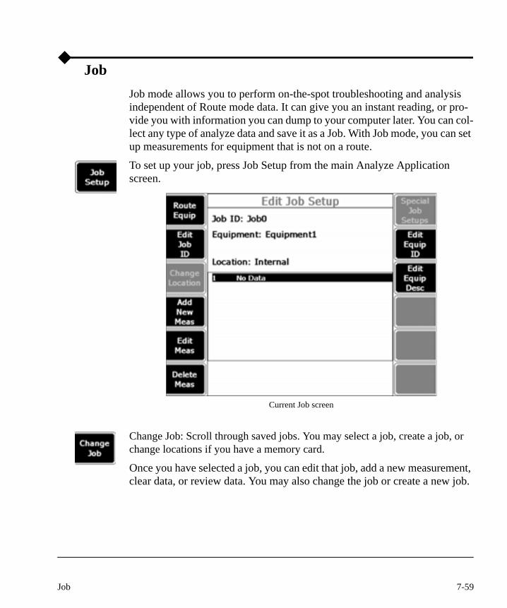
JobJob mode allows you to perform on-the-spot troubleshooting and analysis independent of Route mode data. It can give you an instant reading, or pro-vide you with information you can dump to your computer later. You can col-lect any type of analyze data and save it as a Job. With Job mode, you can set up measurements for equipment that is not on a route.
To set up your job, press Job Setup from the main Analyze Application screen.
Current Job screen
Change Job: Scroll through saved jobs. You may select a job, create a job, or change locations if you have a memory card.
Once you have selected a job, you can edit that job, add a new measurement, clear data, or review data. You may also change the job or create a new job.
7-59Job
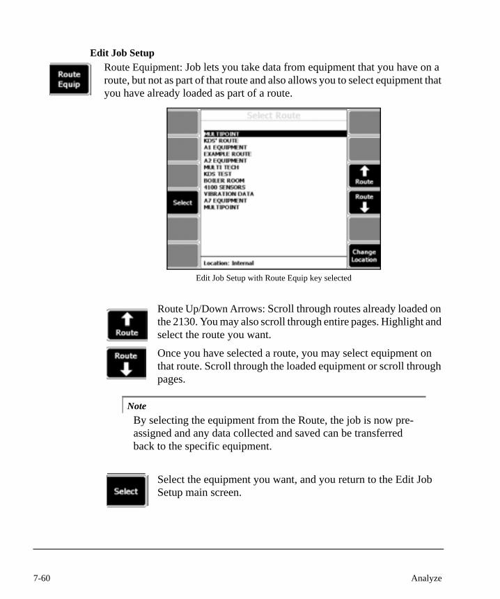
Edit Job SetupRoute Equipment: Job lets you take data from equipment that you have on a route, but not as part of that route and also allows you to select equipment that you have already loaded as part of a route.
Edit Job Setup with Route Equip key selected
Route Up/Down Arrows: Scroll through routes already loaded on the 2130. You may also scroll through entire pages. Highlight and select the route you want.
Once you have selected a route, you may select equipment on that route. Scroll through the loaded equipment or scroll through pages.
NoteBy selecting the equipment from the Route, the job is now pre-assigned and any data collected and saved can be transferred back to the specific equipment.
Select the equipment you want, and you return to the Edit Job Setup main screen.
7-60 Analyze

Edit your job’s ID. The screen becomes your keyboard here. The F1 key acts as A, B, C and 1-- press the key quickly to scroll through the four options (for example, three quick presses to get to C), and pause for five seconds to hold your choice and move to the next letter. Press the ALT key for more functions, such as Insert Over, Start, End, Backspace and Clear All. Press enter once you have finished.
Change Location: If you have one or more memory cards loaded into the ana-lyzer, the Change Location key appears. this key allows you to select a memory card from which to create a new Job or move an existing Job. If you have a CSI 2130 with one card slot, you will not see this option.
Add New Meas: Add a new measurement to your Job.
Edit Meas: Edit the information about a measurement point. you are allowed a maximum of three characters to describe your measurement point. An example point identification might be “MOH,” an abbreviation for motor out-board horizontal.
Delete Meas: Delete a measurement point. A warning screen comes up to make sure that you don’t inadvertently/accidentally delete a point and all of its corresponding data.
Edit Equip ID: Edit your measurement equipment ID. This name can be a maximum of 10 characters.
Meas Up/Down Arrows: Scroll through measurement points already stored on the 2130. You may also scroll through entire pages. Highlight and select the measurement point you want.
Press Enter when you’ve finished editing point information.
7-61Job

Delete Meas: Delete a measurement point. A warning screen comes up to make sure that you don’t inadvertently/accidentally delete a point and all of its corresponding data.
Edit Equip ID: Edit your measurement equipment ID. This name can be a maximum of 10 characters.
Edit Equip Descript: Edit an equipment’s description. You are allowed a max-imum of 28 characters to describe your equipment.
Point Scroll: Use these scroll keys to scroll through your list of measurements.
Press Enter button when you've finished editing your job setup.This returns you to the current job screen.
Create a new job: This brings you to Edit Job Setup screen. Once you've set up a job, press enter and go to manual analyze. From manual analyze, choose what kind of information you want (waveform, orbit, etc).
Review Data: Takes you back to the last data you collected in analyze. You can still store this information to a point, even if it is old (however, any new information is going to replace old information).
Connect for Transfer: Dumping Jobs
If you want to save any Analyze information from your 2130 to use with AMS Machinery Manager, you must attach that information to a job or a route.
You can Connect for Transfer via serial, Ethernet or USB ports. You must choose a specific location to save your job.
7-62 Analyze

Refer to Chapter Three, the communications section of this manual, for more information about dumping your job to your computer or network.
When you have taken measurements on your job or route points, you can transfer the data back to your computer for further analysis. From the main analysis application menu, press ALT to get the secondary menu. Notice the Dump Jobs icon. Make sure you have already attached your USB cable, Ethernet card, or serial port (depending on which you prefer to use) and have set the connection port in the communications setup in the Shell.
Press Connect for Transfer. The analyzer attempts to communicate with your computer. Notice the status bar in the middle of the screen.
You can dump your jobs to your computer using the analyzer.
If you are using an Ethernet connection, and the screen reads “Status: Con-nected,” press the Dump Data key. This brings you to the User Login Config-uration page. You must enter your company name, user login name, and password. Store your login so you don’t have to re-enter this information every time you want to dump. You will be asked to enter a 4-digit pin.Choose a pin number that is simple to type and easy to remember. Press enter to have the analyzer accept your pin.
The next time you need to dump data and get to the user login configuration screen, you can just press Recall Login key; type in your 4-digit pin, and the analyzer will automatically recall your company name, user login, and pass-word.
7-63Job

If using USB or Serial connections, you should connect without having to type in a user name and password.
Once you’ve logged in successfully, you return to the PC communications page. Notice on the second half of the page you can scroll through the jobs saved on the analyzer. Scroll through the jobs, and press Select to put a check-mark next to any job you want to dump. After selecting all the jobs you want to dump press the Begin Data Dump key.
Once all Jobs have been transferred to the database, you can press the Back-space button to disconnect, press the Reset button to return to Analyze, or unplug the USB cable.
5
F1 - Select: Use this key select jobs to transfer to the database.
F3 - Select All: Use this key to select all available jobs to transfer to the database.
F4 - Clear All: Use this key to deselect all previously selected jobs.
F6 - Clear Database Information: If a job as already been transferred to a database, use this key to clear the database name. This will allow the job to be transferred to another database or another PC.
F7 - Begin Data Dump: Use this key to begin the job transfer.
F8 and F9 - Up/Down: These keys will scroll through the list of stored jobs available for transfer.
7-64 Analyze
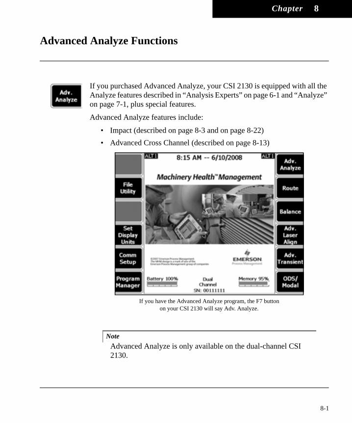
Chapter 8
Advanced Analyze Functions
If you purchased Advanced Analyze, your CSI 2130 is equipped with all the Analyze features described in “Analysis Experts” on page 6-1 and “Analyze” on page 7-1, plus special features.
Advanced Analyze features include:
• Impact (described on page 8-3 and on page 8-22)• Advanced Cross Channel (described on page 8-13)
If you have the Advanced Analyze program, the F7 buttonon your CSI 2130 will say Adv. Analyze.
NoteAdvanced Analyze is only available on the dual-channel CSI 2130.
8-1
Analyze Mode
Press Manual Analyze from the main Analyze Application screen. This brings you to the Analyze Setup screen.
8-2 Advanced Analyze Functions

Impact testing
Analyze Mode Impact screen.
Press Set Analyze Mode and choose Impact from the dropdown list.
Press Enter to go back to the Analyze Setup screen.
8-3Impact testing

Analyze Setup for Impact Mode
Set Spectra Params: The default setting for Impact is Fmax 1000Hz, Fmin 0.0 Hz, Lines: 400. For more information about setting spectra parameters, see “Setting Spectrum Parameters” on page 7-17.
Set Averaging: The default setting for Impact is 4 averages. This would mean impacting the machine four times when collecting data. For more information about setting averages, see “Set Averaging” on page 7-20.
Set Window: The default setting for Impact is a force/exponential window.
The Window parameter applies a shaping function to the waveform data before computing the FFT. Impact testing normally requires two window types. A force window is applied to the hammer channel and an exponential window is applied to the response channel. Selecting the force/exponential window type automatically applies these window types to the appropriate data.
The uniform window does not apply any shaping and is subject to leakage and amplitude errors. The uniform window can be used when analyzing transient signals that are completely contained within the analysis time record length.
8-4 Advanced Analyze Functions

You may have to perform a few sample measurements to configure the force/exponential window correctly. The options are:
Window Force/Exponential
Start Time Should be equal or slightly less than the percent pre-trigger in the Set Trigger menu. A good default value for Pre Trigger is 10%, Start Time 9%, until other window parameters are determined.
Force Width The duration of the force signal, expressed as a percentage of the overall sampling time. It requires initial test measurements in order to determine the actual force duration relative to the overall sampling time. 10% is a good default value.
COS Taper A feature that “smooths” the leading edge of both the force and exponential window and the trailing edge of the force window. A value of 10-20% is recommended.
Expo Decay Value at which amplitude has decreased by 1/e, where e= 2.7182. This should occur at 1/4 of the total time record, so a value of 20-25% is a good start.98% is the maximum value that can be entered. If you enter “zero,” you prompt the machine to automatically calculate a decay value.
8-5Impact testing
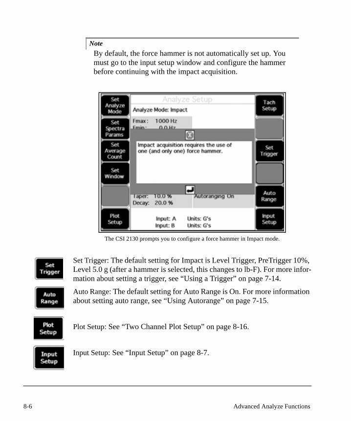
NoteBy default, the force hammer is not automatically set up. You must go to the input setup window and configure the hammer before continuing with the impact acquisition.
The CSI 2130 prompts you to configure a force hammer in Impact mode.
Set Trigger: The default setting for Impact is Level Trigger, PreTrigger 10%, Level 5.0 g (after a hammer is selected, this changes to lb-F). For more infor-mation about setting a trigger, see “Using a Trigger” on page 7-14.
Auto Range: The default setting for Auto Range is On. For more information about setting auto range, see “Using Autorange” on page 7-15.
Plot Setup: See “Two Channel Plot Setup” on page 8-16.
Input Setup: See “Input Setup” on page 8-7.
8-6 Advanced Analyze Functions

Input Setup
Input Setup screen with force hammer parameters
Input Setup lets you configure the parameters for your input sources. For more information about Input Setup, see “Using Input Setup” on page 7-15.
Analyze Input Setup defaults to Input: A and B in both Impact and Advanced Cross Channel modes.
• Press Enter to return to the Input Setup Screen. • Press Set Data Units if you need to change the units of measurement. • Press Enter to return to the Analyze Setup screen.
8-7Impact testing
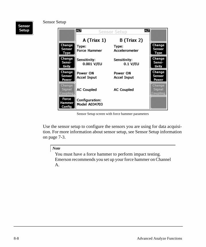
Sensor Setup
Sensor Setup screen with force hammer parameters
Use the sensor setup to configure the sensors you are using for data acquisi-tion. For more information about sensor setup, see Sensor Setup information on page 7-3.
NoteYou must have a force hammer to perform impact testing. Emerson recommends you set up your force hammer on Channel A.
8-8 Advanced Analyze Functions
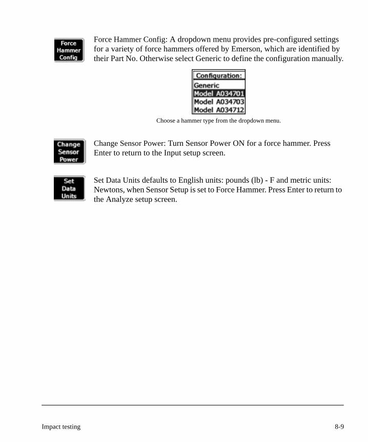
Force Hammer Config: A dropdown menu provides pre-configured settings for a variety of force hammers offered by Emerson, which are identified by their Part No. Otherwise select Generic to define the configuration manually.
Choose a hammer type from the dropdown menu.
Change Sensor Power: Turn Sensor Power ON for a force hammer. Press Enter to return to the Input setup screen.
Set Data Units defaults to English units: pounds (lb) - F and metric units: Newtons, when Sensor Setup is set to Force Hammer. Press Enter to return to the Analyze setup screen.
8-9Impact testing

Impact Acquisition Process
Place the sensor on the structure. A stud or magnetic mount is recommended.
Press Enter from the Analyze Setup screen to start data acquisition. In a few seconds, the message “Strike with force hammer,” appears at the bottom of the screen.
At this time, strike the structure with a hammer at a location that is two to four feet away from where the sensor is mounted.
Until the first strike is made, the analyzer’s front panel LED flashes green (about once per second) and beeps (if the keypad beeper is on). Press Enter, Reset, or Stop to abort the acquisition and return to the Analyze screen.
Once you have made the first strike with the force hammer, the data for the first average (1 of 4 in the example), displays.
The data for your first average displays after you make the first strike.
8-10 Advanced Analyze Functions
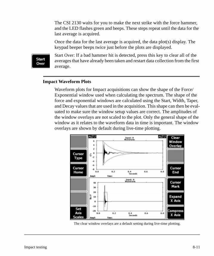
The CSI 2130 waits for you to make the next strike with the force hammer, and the LED flashes green and beeps. These steps repeat until the data for the last average is acquired.
Once the data for the last average is acquired, the data plot(s) display. The keypad beeper beeps twice just before the plots are displayed.
Start Over: If a bad hammer hit is detected, press this key to clear all of the averages that have already been taken and restart data collection from the first average.
Impact Waveform Plots
Waveform plots for Impact acquisitions can show the shape of the Force/Exponential window used when calculating the spectrum. The shape of the force and exponential windows are calculated using the Start, Width, Taper, and Decay values that are used in the acquisition. This shape can then be eval-uated to make sure the window setup values are correct. The amplitudes of the window overlays are not scaled to the plot. Only the general shape of the window as it relates to the waveform data in time is important. The window overlays are shown by default during live-time plotting.
The clear window overlays are a default setting during live-time plotting.
8-11Impact testing

Clear Window Overlay: Removes the window overlays from all waveform plots.
Display Window Overlay: Draws the window overlays on all of the waveform plots.
8-12 Advanced Analyze Functions

Advanced Cross Channel Testing
Analyze Mode Advanced Cross Channel screen.
Press Set Analyze Mode and choose Adv. Cross Channel from the dropdown list.
Press Return to go back to the Analyze Setup screen.
8-13Advanced Cross Channel Testing
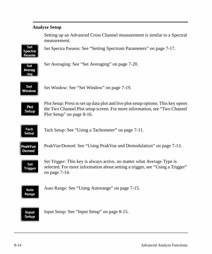
Analyze Setup
Setting up an Advanced Cross Channel measurement is similar to a Spectral measurement.
Set Spectra Params: See “Setting Spectrum Parameters” on page 7-17.
Set Averaging: See “Set Averaging” on page 7-20.
Set Window: See “Set Window” on page 7-19.
Plot Setup: Press to set up data plot and live plot setup options. This key opens the Two Channel Plot setup screen. For more information, see “Two Channel Plot Setup” on page 8-16.
Tach Setup: See “Using a Tachometer” on page 7-11.
PeakVue/Demod: See “Using PeakVue and Demodulation” on page 7-13.
Set Trigger: This key is always active, no matter what Average Type is selected. For more information about setting a trigger, see “Using a Trigger” on page 7-14.
Auto Range: See “Using Autorange” on page 7-15.
Input Setup: See “Input Setup” on page 8-15.
8-14 Advanced Analyze Functions

Input Setup
Input Setup for Advanced Cross Channel.
Input Setup lets you configure the parameters for your input sources. For more information about Input Setup, see “Using Input Setup” on page 7-15.
Sensor Setup: The sensor input automatically defaults to the dual channel A and B option in Advanced Cross Channel mode. If the units are displayed in G’s, that means both sensors are set to accelerometers.
Both input sensors are set to accelerometers in this example.
8-15Advanced Cross Channel Testing

Two Channel Plot SetupPress Plot Setup from the Analyze Setup screen to open the Two Channel Plot setup. Two Channel Plot Setup is only available if your analyze mode is set to Impact or Advanced Cross Channel.
With Two Channel Plot Setup, you can select the type of data plots you want to display during and after data acquisition.
Two Channel Plot Setup screen.
8-16 Advanced Analyze Functions

Set Plot, Force Hammer SelectedIf the Force Hammer is selected, this dropdown menu appears. Highlight the selection you need and press Enter.
Set Plot dropdown menu, if Force Hammer is selected.
Set Plot, No Force HammerIf no Force Hammer is selected, this dropdown menu appears. Highlight the selection you need and press Enter.
Set Plot dropdown menu, if Force Hammer is not selected.
8-17Two Channel Plot Setup

Set Plot Options Explained
Frequency Response Functions (FRF): FRF plots display like a spectrum, except you cannot list peaks.
The A/B FRF transfer function is the amount of force that is required to pro-vide a response at a given frequency. It is also the measure of Force/Output.
Three types of A/B FRF plots can be displayed during an impact acquisition (depending on the sensor setup). See the table on page 8-19 for more infor-mation.
The B/A FRF transfer function is the measured ratio of response of the struc-ture acceleration to a known excitation. It is also the measure of Output/Force.
Three types of B/A FRF plots can by displayed during an impact acquisition (depending on the sensor setup).
Waveform- Input: A Displays the waveform from the A channel signal
Waveform- Input: B Displays the waveform from the B channel signal
Spectrum- Input A Displays the spectrum from the A channel signal
Spectrum- Input B Displays the spectrum from the B channel signal
Coherence Describes the degree of linear relationship between to signals
Cross Channel Phase Displays the phase relationship of the channel A and channel B signals
A/B FRF Displays a spectrum representing the transfer function of channel A / channel B
B/A FRF Displays a spectrum representing the transfer function of channel B / channel A
8-18 Advanced Analyze Functions
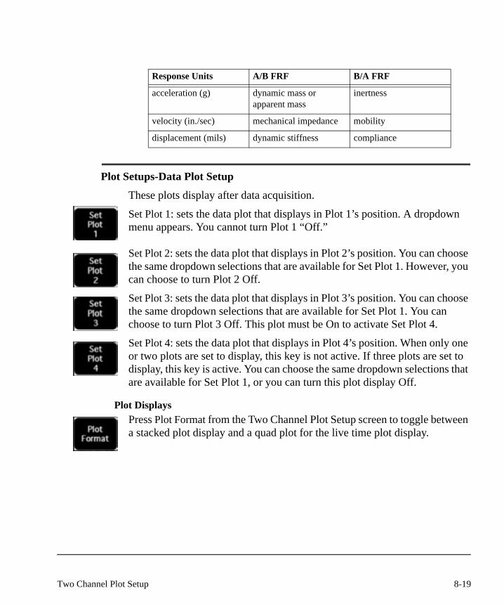
Plot Setups-Data Plot Setup
These plots display after data acquisition.
Set Plot 1: sets the data plot that displays in Plot 1’s position. A dropdown menu appears. You cannot turn Plot 1 “Off.”
Set Plot 2: sets the data plot that displays in Plot 2’s position. You can choose the same dropdown selections that are available for Set Plot 1. However, you can choose to turn Plot 2 Off.
Set Plot 3: sets the data plot that displays in Plot 3’s position. You can choose the same dropdown selections that are available for Set Plot 1. You can choose to turn Plot 3 Off. This plot must be On to activate Set Plot 4.
Set Plot 4: sets the data plot that displays in Plot 4’s position. When only one or two plots are set to display, this key is not active. If three plots are set to display, this key is active. You can choose the same dropdown selections that are available for Set Plot 1, or you can turn this plot display Off.
Plot DisplaysPress Plot Format from the Two Channel Plot Setup screen to toggle between a stacked plot display and a quad plot for the live time plot display.
Response Units A/B FRF B/A FRF
acceleration (g) dynamic mass or apparent mass
inertness
velocity (in./sec) mechanical impedance mobility
displacement (mils) dynamic stiffness compliance
8-19Two Channel Plot Setup

The stacked plot option displays plots the width of the display area, stacked on top of each other.
Three plots are in a stacked display.
8-20 Advanced Analyze Functions

The quad plot shows four plots in the quarters of the screen.
Four plots are in the quad display.
Plot Setups-Live Plot Setup
These plots display during data acquisition.
Set Plot 1: If the analyze mode is set to Advanced Cross Channel or Impact modes, the dropdown menus on page 8-17 displays. You can turn this plot Off.
Set Plot 2: Is only active if Set Plot 1 is activated. When active, Plot 2 displays a live time plot. Configure this plot with the menu items listed on page 8-17. You can turn this plot Off.
Set Plot 3: Is only active if Set Plot 2 is activated. When active, Plot 3 displays a live time plot. Configure this plot with the menu items listed on page 8-17. You can turn this plot Off.
Set Plot 4: Is only active if Set Plot 3 is activated. When active, Plot 4 displays a live time plot. Configure this plot with the menu items listed on page 8-17. You can turn this plot Off.
8-21Two Channel Plot Setup

Applications and Insights Related to Impact TestingIf you are new to this method of testing for machine resonance, please read this entire section before performing your first impact test. This chapter was written with the beginner in mind and doesn’t detail the theory of impact testing, but rather focuses on what you really need to know to successfully perform resonance tests.
Why perform an impact test?Impact testing determines the presence of resonant frequencies. An impact test can also find structural cracks and measure the dynamic stiffness of a structure.
What does the impact do to the machine?If you impact a machine by hitting it with a rubber mallet, you create a type of vibration that contains many vibration frequencies. Impacts are the stan-dard excitation force for measurement of resonant frequencies.
What’s a resonant frequency?Most structures have a resonant frequency. A resonant frequency is a natural frequency of vibration that is determined by the physical parameters of the vibrating object. The damping of mechanical vibrations in the structure at res-onant frequency is very weak.
It is easy to get an object to vibrate at its resonant frequencies, and once an object reaches resonant frequency, it takes a long time to decay. This can amplify the severity of other vibration sources, such as imbalance or mis-alignment.
How do I measure a resonant frequency?To measure the resonant frequency, excite the structure with a vibration source that contains a mixture of many frequencies. The frequencies that are near the resonance take longer to decay than other frequencies, and the struc-ture will “ring” at this resonant frequency. Use the CSI 2130 to analyze the ringing frequency that corresponds to the resonant frequency.
8-22 Advanced Analyze Functions

Should I use single-channel or dual-channel measurement?A single-channel measurement can only record the impact and identify the resonant frequency (or frequencies) of a structure. Use a dual-channel mea-surement to measure the amplification of a resonant frequency, determine stiffness and damping, and confirm that the recorded frequency is a resonance and no other background vibration.
A dual-channel measurement records the amount of force applied with an instrumented force hammer on one channel and records the response on the second channel.
A dual-channel CSI 2130 with the Advanced Two Channel special purpose program and an instrumented force hammer is required for dual-channel impact testing.
Understanding Impact Testing
The Impact TestTwo-channel impact testing is a fairly straightforward way to determine the resonant frequencies of machines, machine foundations, and other structures. Other methods exist, such as start-up or coast-down tests, single-channel “bump” tests, and resonance tests done with a shaker. However, these methods have analysis limitations that when performed individually, may not conclusively identify resonance.
1
8-23Applications and Insights Related to Impact Testing
Resonance Explained Resonance is a condition that occurs when a resonant frequency (sometimes called a natural frequency) is excited by an external forcing frequency.
The forcing frequency is amplified by the resonant frequency—the frequency at which a machine will naturally amplify vibration when excited. For example, a bell always possess the ability to vibrate at its resonant frequency. It will not sound until it is struck with the correct mallet.
All structures possess resonance, and just because a machine has a resonant frequency, that does not mean that the machine is faulty. Resonance is only a problem when a forcing frequency, such as one times the turning speed (TS), coincides with a resonant frequency. Often, if a machine is exhibiting very high vibration the analyst must answer the question “Is the machine shaking because it is way out of balance or is the machine shaking due to a small amount of unbalance that is exciting a resonance?”
There are several measurements that can be made while a machine is oper-ating to initially identify resonance such as a negative linear averaging bump test, phase measurements between the horizontal and vertical directions being 0 degrees or 180 degrees out of phase with a 90 degree shift in the direction of the sensor. Again, these tests can point to or suggest resonance, but the two-channel impact test using an instrumented force hammer and a response sensor such as an accelerometer will conclusively prove or disprove the pres-ence of a resonant frequency.
How Impact Testing WorksImpact testing is usually easier to use for most medium to light structures. Heavy structures such as locomotive engines, large multi-story structures, and satellites do not respond as well to impacting and often require more complex excitation methods such as dynamic shaker excitation or snap-back testing.
The impact test places a small amount of input force into a specific frequency range. Although the hammer impact may show a value of 100 pounds of force in the time waveform data, less than one pound of force will be input into the structure at each frequency. Different hammer designs exist and should be selected for the different types of structures.
8-24 Advanced Analyze Functions
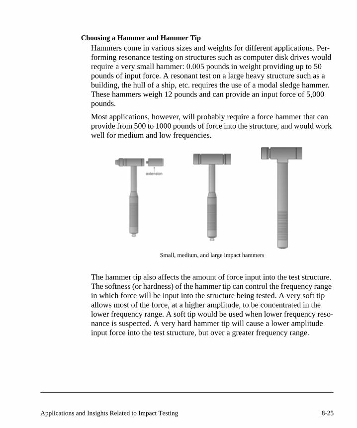
Choosing a Hammer and Hammer TipHammers come in various sizes and weights for different applications. Per-forming resonance testing on structures such as computer disk drives would require a very small hammer: 0.005 pounds in weight providing up to 50 pounds of input force. A resonant test on a large heavy structure such as a building, the hull of a ship, etc. requires the use of a modal sledge hammer. These hammers weigh 12 pounds and can provide an input force of 5,000 pounds.
Most applications, however, will probably require a force hammer that can provide from 500 to 1000 pounds of force into the structure, and would work well for medium and low frequencies.
Small, medium, and large impact hammers
The hammer tip also affects the amount of force input into the test structure. The softness (or hardness) of the hammer tip can control the frequency range in which force will be input into the structure being tested. A very soft tip allows most of the force, at a higher amplitude, to be concentrated in the lower frequency range. A soft tip would be used when lower frequency reso-nance is suspected. A very hard hammer tip will cause a lower amplitude input force into the test structure, but over a greater frequency range.
8-25Applications and Insights Related to Impact Testing

The harder tips should be used when higher frequency resonances are sus-pected. If you want to try this yourself, take a bell and impact it with a soft tennis ball and then with something harder like a baseball and notice the dif-ference in the sound of the bell. Generally, the harder baseball has excited the higher frequencies of the bell and the tennis ball will have excited the lower frequencies of the bell.
Hammer tip data plot.
When choosing the right hammer tip for the job, examine the spectrum of the hammer impact. The frequency range of the input force can be observed in the spectrum of the hammer impact. If necessary, try different tips until a tip that provides the input force over the correct frequency range is found.
Two-Channel Verses Single-Channel TestingFor years, people with a single-channel analyzer have been able to perform “bump tests.” These test are a good first indication as to whether a structure may be resonant at or near equipment forcing frequencies. However, since there is no way to measure the relationship between the hammer blow and the vibration sensor’s response, you cannot be really sure the vibration measured by the sensor was caused by the hammer.
The vibration sensor may pick up vibration from nearby machinery that is still running, other impacts occurring in the plant may cause the structure nearby to shake at its natural frequency, and so on. If a single-channel ana-lyzer is used for resonance testing then other single-channel resonance tests should be performed in addition to the bump test.
8-26 Advanced Analyze Functions

The two-channel impact test can definitively measure the resonant frequen-cies of a structure. This test has the capability of measuring not only the output of the system measured at the vibration sensor, but also the input force at the hammer. The two-channel analyzer in the Advanced Two-Channel downloadable program can calculate the relationships between the hammer and the vibration sensor. The three most important measurements to the field analyst are the frequency response function (FRF), cross-channel phase, and the cross-channel coherence.
Simply put, the FRF displays the frequency of the resonance, the phase plot identifies the phase shift at the suspected resonant frequency, and the coher-ence plot provides the data validity information.
Definitions of Frequency Response Function, Phase, and CoherenceThe Frequency Response Function is defined as the Fourier transform of the output signal divided by the Fourier transform of the input signal. For the CSI 2130, the hammer is considered the input signal and should be connected to channel A. An accelerometer should be used for the output (or response) and should be connected to channel B. The FRF measurement would then be output divided by input, or channel B divided by channel A. This type of FRF measurement is sometimes called “Inertance” or “Accelerance.”
In an inertance plot, a resonant frequency will be observed as a peak in the spectral data plot. There are actually six different FRF measurements that can be made or calculated from the inertance measurement.
Frequency Response Function Data Type (Units) Resonance
Inertance Acceleration/Force (G’s/LBF) Peak
Mobility Velocity/Force (IPS/LBF) Peak
Compliance Displacement/Force (MIL/LBF) Peak
Effective Mass Force/Acceleration (LBF/G’s) Valley
Impedance Force/Velocity (LBF/IPS) Valley
Dynamic Stiffness Force/Displacement (LBF/MIL) Valley
8-27Applications and Insights Related to Impact Testing

The phase measurement provides the phase difference at each line of resolu-tion. Phase is important because at resonance the phase will shift approxi-mately 180 degrees if the structure is lightly damped. A less than 180 degree phase shift could mean that the structure is more heavily damped or that the structure’s motion at the resonant frequency is not primarily in the direction of the accelerometer and/or the hammer.
Coherence measurement is critical to the Impact testing validation. Coher-ence is a measure of how much of the output vibration was caused by the input force. If all of the output vibration was caused by the input force, the coherence will be at a value of 1.0 (or very close to 1.0) It is almost impos-sible to achieve a value of 1.0 (perfect coherence) over the entire frequency range.
Fortunately, the test can be considered valid as long as the coherence is greater than 0.75. If the coherence is less than 0.75, then it is possible that the response is being caused by other vibration inputs besides the input force hammer being used in the test. The coherence is an averaged function and its value will always be 1.0 after the first impact. Generally, four to six averages should be taken at each measurement location.
Drive Point Measurements and Transfer Point MeasurementsWhen the vibration sensor is placed at the same location as the hammer impact point, this measurement is called a drive point. Each combination of resonance testing measurements should always include a drive point mea-surement. If the data is going to used in a modal analysis software package, then a drive point measurement is absolutely critical.
2
8-28 Advanced Analyze Functions
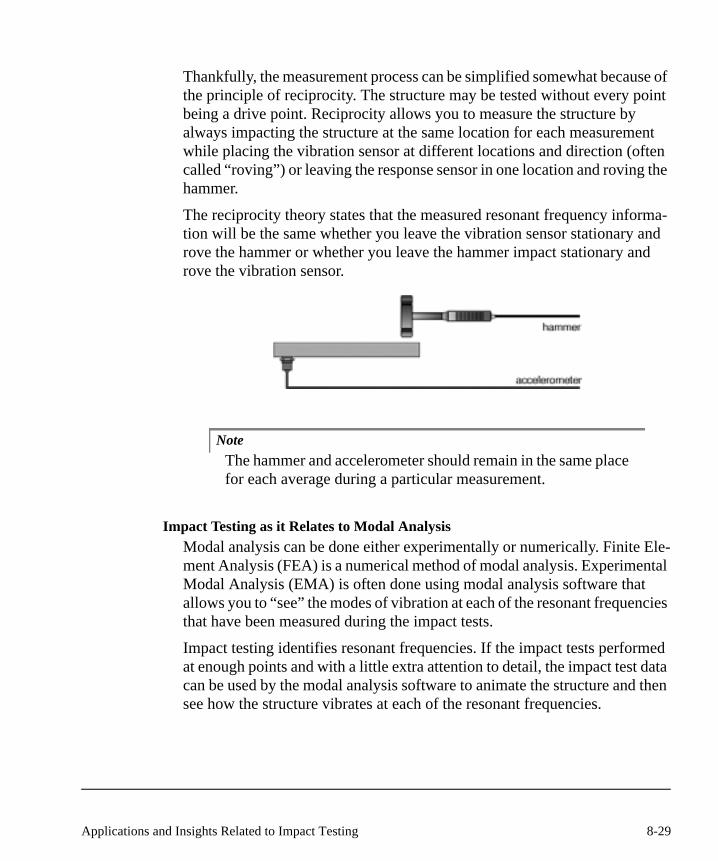
Thankfully, the measurement process can be simplified somewhat because of the principle of reciprocity. The structure may be tested without every point being a drive point. Reciprocity allows you to measure the structure by always impacting the structure at the same location for each measurement while placing the vibration sensor at different locations and direction (often called “roving”) or leaving the response sensor in one location and roving the hammer.
The reciprocity theory states that the measured resonant frequency informa-tion will be the same whether you leave the vibration sensor stationary and rove the hammer or whether you leave the hammer impact stationary and rove the vibration sensor.
3
NoteThe hammer and accelerometer should remain in the same place for each average during a particular measurement.
Impact Testing as it Relates to Modal AnalysisModal analysis can be done either experimentally or numerically. Finite Ele-ment Analysis (FEA) is a numerical method of modal analysis. Experimental Modal Analysis (EMA) is often done using modal analysis software that allows you to “see” the modes of vibration at each of the resonant frequencies that have been measured during the impact tests.
Impact testing identifies resonant frequencies. If the impact tests performed at enough points and with a little extra attention to detail, the impact test data can be used by the modal analysis software to animate the structure and then see how the structure vibrates at each of the resonant frequencies.
8-29Applications and Insights Related to Impact Testing
Testing performed only to identify resonant frequencies, and not in support of a modal analysis study, can usually be accomplished with a few measurement points. Modal analysis often involves 10 or more measurement locations measured horizontally, vertically, and/or axially.
The remainder of this chapter focuses on how to best capture quality impact test data as it relates to identifying resonant frequencies. A full discussion of experimental modal analysis is outside the scope of this user manual.
Preliminary Testing Considerations
Have a PlanIt is important for all impact tests to have test procedures in place to correctly identify structure resonance. These test procedures may be written down or not. The experienced analyst will have a goal in mind as to what is to be accomplished with the impact tests that are to be performed.
Most likely, the structure will be tested to identify the presence of resonant frequencies at or near a forcing frequency such as one times the turning speed or its harmonics, one time belt frequency and/or its harmonics, vane or blade pass frequencies, etc.
Determine Frequency Range and Lines of ResolutionFor most testing, a problem has already been suspected based on spectral data collected during routine data collection or other special testing. The recom-mended maximum frequency (Fmax) for your impact test should be roughly two times the highest frequency where you suspect a resonance. For example, if you suspect resonance in the 80 to 100 Hz range, you should collect data to at least 200 Hz.
Experienced analysts may examine the frequency range four to five times above the highest suspected resonant frequency to get a better idea of what the machine is experiencing. Be careful, because your hammer may not put enough energy into the system at higher frequencies to make this measure-ment valid. Do not try to take data above the Fmax of your sensor or above the frequency range of the input force hammer tip.
8-30 Advanced Analyze Functions
For most testing, set the lines of resolution equal to the Fmax in Hz. For example, if the Fmax is set to 400 Hz, choose 400 lines of resolution. This results in a one second time waveform and this works well for most medium to heavy structures.
Lighter structures may need a longer time waveform, that may well mean a lower Fmax and/or more lines of resolution.
Choosing an Accelerometer and a HammerMake sure the right equipment is selected. Select an instrumented force hammer that allows force to be input at adequate amplitudes and in the right frequency range. (See “How Impact Testing Works” on page 8-24.)
Lightweight structures have higher frequency resonances and need light-weight, high-frequency accelerometers. The accelerometers should be attached with a mounting wax or lightweight epoxy. The object is to not change the structure to be measured by adding additional mass from the placement of the sensor. This will usually cause the measured resonance to be lower than the actual resonance due to the added mass of the sensor.
Large heavy structures have lower resonant frequencies and require acceler-ometers that measure in this frequency range. These sensors are often heavier than the sensors used for high frequency testing. This is not a problem since the structure is heavy and the additional mass of a heavier accelerometer will not effect the impact measurement.
If you are unsure, contact your sensor supplier to ensure that you have the cor-rect sensor and hammer for the job. Some firms rent equipment for special impact testing projects that call for equipment that may only be needed occa-sionally.
Exploratory Impacts As the testing begins, you should make some trial runs before data is saved. Ensure that good data will be acquired from the extreme positions of the test structure. In other words, try impacting at one end of the structure while the accelerometer is placed at the other end. The goal here is to ensure that the force transmits through the structure well. Examining the coherence data should indicate how well the force is transmitted. If good force transmission is not occurring, then the response location may need to be moved.
8-31Applications and Insights Related to Impact Testing
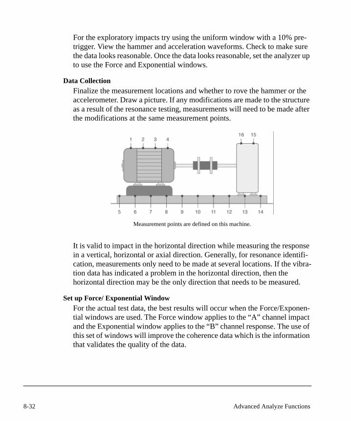
For the exploratory impacts try using the uniform window with a 10% pre-trigger. View the hammer and acceleration waveforms. Check to make sure the data looks reasonable. Once the data looks reasonable, set the analyzer up to use the Force and Exponential windows.
Data CollectionFinalize the measurement locations and whether to rove the hammer or the accelerometer. Draw a picture. If any modifications are made to the structure as a result of the resonance testing, measurements will need to be made after the modifications at the same measurement points.
Measurement points are defined on this machine.
It is valid to impact in the horizontal direction while measuring the response in a vertical, horizontal or axial direction. Generally, for resonance identifi-cation, measurements only need to be made at several locations. If the vibra-tion data has indicated a problem in the horizontal direction, then the horizontal direction may be the only direction that needs to be measured.
Set up Force/ Exponential WindowFor the actual test data, the best results will occur when the Force/Exponen-tial windows are used. The Force window applies to the “A” channel impact and the Exponential window applies to the “B” channel response. The use of this set of windows will improve the coherence data which is the information that validates the quality of the data.
8-32 Advanced Analyze Functions

Recommended Force/Exponential Window Settings(Based on a 10% pre-trigger selection)
The Force width can be decreased if the data appears to have substantial noise in it and the measured coherence is poor. A tighter force window may improve the coherence. Do not, however, narrow the force window to the point that the actual force information is being windowed out of the measure-ment.
The display of the FRF is really one half of the picture; coherence is the other half. Collected data should be displayed with the FRF of acceleration response divided by the force input (B/A) as one plot (usually the upper plot), and the coherence as the other plot (usually displayed as the lower plot). It is the coherence data that validates, or proves, the acceptability of the FRF data.
Remember, resonance is identified as a peak in the FRF. The coherence must be above 0.75 for the data to be considered valid over the frequency ranges of interest. As the cross channel data are averaged functions, the coherence will tend to decrease as the number of averages increases.
When taking the data, take at least four averages—six to eight averages is better. After the measurements have been made, save the data. Label the data making sure the data label matches what you have in your test sketch. Also, make sure it is described well in the analyzer as well as the test sketch. If the data shows a peak in the FRF plot, coherence above 0.75 in the coherence plot, and a phase change approaching 180 degrees in the phase plot, then the data has identified a resonance in the mechanical system.
A coherence value below 0.75 may be an indication of faulty sensor or sensor cable, poor signal processing setup, or non-linear structures due to loose parts or cracks in the structure.
Window Parameter Parameter Value (% of total time record)
Start Time 9
Force Width 10
Cosine Taper 10
Exponential Decay 25
8-33Applications and Insights Related to Impact Testing
Summary
Once a resonant frequency has been confirmed as a problem, the next step is solving the resonance problem.
A resonance cannot be eliminated completely; the solution to a resonance problem is always one of the four things listed below:
• Move the forcing frequency to not coincide with the structures natu-rally present resonant frequency.
• Move the resonant frequency by changing the mass or the stiffness of the structure.
• Add more damping to the structure. (This is often the most difficult solution.)
• Design and install a tuned Dynamic Vibration Absorber (DVA). The first two solutions typically result in the most permanent type of fix. If a five-bladed fan excites a resonance at five times turning speed, then changing to six or seven blades would be an example of changing the forcing fre-quency. Adding mass lowers the resonant frequency and adding stiffness will raise the resonant frequency. Damping absorbs the vibration energy at reso-nance and is often the only solution for variable speed machines. The DVA solution is not always permanent and these devices have been known to break loose from a structure.
Fixing a resonance problem often involves some type of structural redesign that should only be done by qualified personnel. Emerson can recommend qualified specialists to help you in your solution of resonance problems if the expertise to solve these problems does not exist at your facility.
Resonance testing with the two-channel advanced diagnostic downloadable program can be easy, exciting, and beneficial. It puts the power of sophisti-cated testing techniques in the hands of field personnel who can identify sig-nificant structural problems in their own facilities without calling in additional resources from outside the plant.
8-34 Advanced Analyze Functions

Chapter 9
Advanced Transient
What is Advanced Transient?Advanced transient allows acquisition of large unbroken time waveforms, similar to a digital tape recorder. A stored time waveform can then be post-processed to generate a spectrum from any section of the waveform.
The 2130 Advanced Transient Analysis program extends the advanced diag-nostic capabilities of the CSI Model 2130 Machine Analyzer. This program enables the Model 2130 Analyzer to simultaneously collect a continuous time waveform from up to two input channels. Although the input signal can be from any compatible dynamic transducer, vibration is most commonly measured.
Transient analysis is typically used by machine analysts who want to investigate the behavior of a machine under varying (transient) conditions, such as during speed or load changes. This application is a very useful tool when troubleshooting repetitive machining operations such as boring or grinding. The fundamental procedure consists of collecting the time waveform over the period of time when an event of interest is likely to occur, such as during one complete cycle of a machining operation, during a process change on a compressor, or during the coastdown of a machine rotor, etc. After the data has been acquired it may then be examined for any changes in pattern, frequency, or amplitude that are of interest. These “events” will then be analyzed to reveal how the machine is responding to these transient events or what is causing these events to occur.
Emerson’s patented PeakVue® technology can be applied to the input signal while acquiring the transient waveform. Transient waveforms can be post processed by the Model 2130 Analyzer to expand the display on specific time segments of interest. Selected time segments may be displayed as frequency and amplitude spectra (FFTs) using from 200 to 6400 lines of resolution.
A video tutorial about the configuration and use of the CSI2130 Advanced transient application can be found at: http://www.compsys.com/technology/CSI2130/CSI2130_inettools.html.
9-1
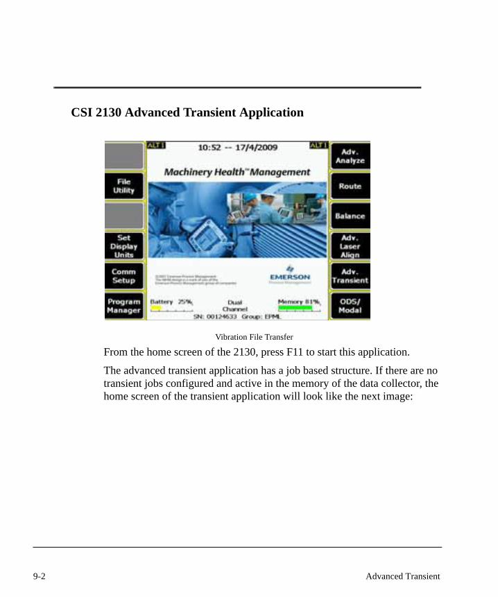
CSI 2130 Advanced Transient Application
Vibration File Transfer
From the home screen of the 2130, press F11 to start this application.
The advanced transient application has a job based structure. If there are no transient jobs configured and active in the memory of the data collector, the home screen of the transient application will look like the next image:
9-2 Advanced Transient

All other functionalities are grey out as long as there is not at least 1 job con-figured. If the advanced transient application has started, and a job configured in the active memory, the home screen of the advanced transient application will look like:
9-3
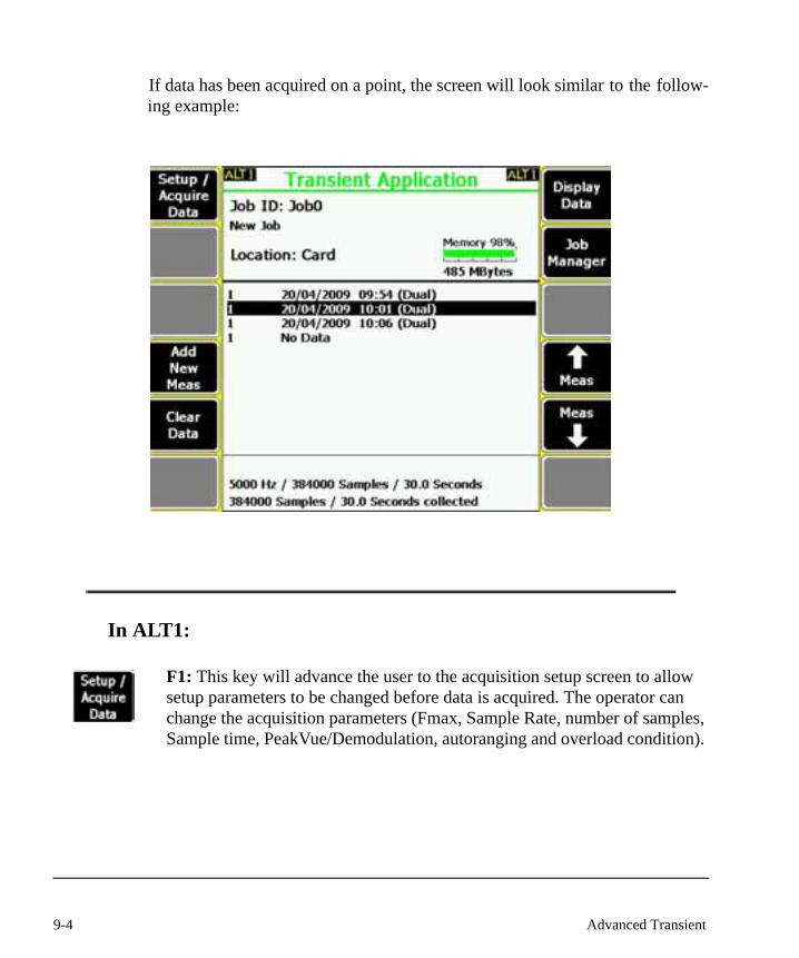
If data has been acquired on a point, the screen will look similar to the follow-ing example:
In ALT1:
F1: This key will advance the user to the acquisition setup screen to allow setup parameters to be changed before data is acquired. The operator can change the acquisition parameters (Fmax, Sample Rate, number of samples, Sample time, PeakVue/Demodulation, autoranging and overload condition).
9-4 Advanced Transient

Before going to the setup screen, if data has been acquired on this measure-ment, the operator is asked if previously acquired data is to be deleted. If the answer is no, then the setup screen is displayed, but no parameters may be changed. The operator has to exit with the “Back” key. If the answer is yes, then the data is deleted (deleted data is not recoverable) and the setup screen is displayed.
F4: This key allows the operator to add another measurement to the job. The setup for the new acquisition is not defined. When the operator goes to acquire data for the first time on a measurement, the setup will be the same as the last acquisition or the setup from the last reviewed acquisition.
Before adding the new measurement, the application checks to make sure there is enough memory to add a new measurement. A warning message will appear if there is not enough memory for a new measurement.
F5: This key is active only if data has been acquired on the active measure-ment. If any data has been acquired for this measurement and the key is pressed, then the application will ask the operator if the data is really meant to be cleared. Press “Back” for No or press “Enter” for Yes. If the operator answers Yes, then the application will clear (delete) the data. When deleting data from a measurement, any setup parameters stored on the measurement are not deleted.
Caution!Use extreme caution when using the Clear Data function when the analyzer contains important collected data. After answering Yes, the data can not be retrieved.
F7: This key is only active if data has been acquired on the highlighted mea-surement. If data has been acquired, the application will display the data forthe current Measurement.
F8 Job Manager: This key takes the operator to the job manager routines.From here, the operator can select jobs, edit jobs, change memory locationto/from external memory cards, or transfer jobs to a host computer.
9-5

The job manager mode is explained in detail starting from page 7-55.
F10 and F11: The Measurement Up and MeasurementDown keys are used to highlight (select) a measurement. These keys movethrough the list of measurements one measurement at a time. Measurementselection auto repeats and accelerates if these keys are held down. The Up andDown arrow keys will do the same.
Information on the highlighted measurement is displayed on 3 lines on the bot-tom of the screen.
The first line displays the measurement description, if one is required to beentered into the description field.
If data has been acquired or a setup defined for this measurement, the secondline displays acquisition parameters (Fmax, number of samples, sample time).
If data has been acquired for this measurement, the third line displays the actualnumber of samples acquired and actual time of acquisition.
Note
9-6 Advanced Transient

In ALT2:
F3: This key takes the operator to the Sensor setup screen. This is the same sen-sor Setup as in the Manual Analyze application. Here the operator can setupSensor Type, Sensor Sensitivity, Sensor Power On/Off, Signal Coupling andAccelerometer Configuration. More details can be found on page 7-3.
F4: This key takes you to the Tach Setup screen. This is the same Tach Setup asin Analyze (more details are on page 7-10). Parameters that can be modifiedinclude: Pseudo Tach Enabled/Disabled, Tach Power On/Off, Trigger Level,Edge Delay and RPM display.
F5: This key takes the operator to the Data Display Settings screen. The DataDisplay Settings displayed and edited here are global parameters and are globalsettings used each time data is viewed. The following parameters can be sethere: number of points, number of lines, window type, spectrum units and showtach times.
F6: If there are more than two plots available, this key will start the Select Plotscreen that will set which plot or plots will be displayed. The format for display-ing multiple plots can also be set. Formats selected here will be global parame-ters and used each time plot routines are started.
9-7

F7: This key will end the “Transient” application and return to the home screen.
9-8 Advanced Transient
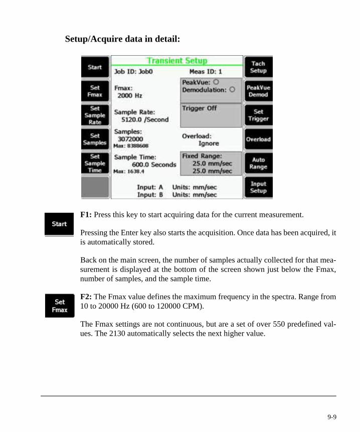
Setup/Acquire data in detail:
F1: Press this key to start acquiring data for the current measurement.
Pressing the Enter key also starts the acquisition. Once data has been acquired, itis automatically stored.
Back on the main screen, the number of samples actually collected for that mea-surement is displayed at the bottom of the screen shown just below the Fmax,number of samples, and the sample time.
F2: The Fmax value defines the maximum frequency in the spectra. Range from10 to 20000 Hz (600 to 120000 CPM).
The Fmax settings are not continuous, but are a set of over 550 predefined val-ues. The 2130 automatically selects the next higher value.
9-9

Changing Fmax adjusts the Sample Rate as they are related. Fmax = (SampleRate)/(2.56). In addition, changing Fmax will change the Sample Time, butchanging the Sample Time does not change Fmax. Fmax = (Number of Sam-ples)/(2.56*Sample Time)
F3: The Sample Rate value defines the rate of acquisition in number of samplesper second. Values may range from 25.6 to 51200. Setting the Sample Rateautomatically adjusts Fmax: Sample Rate = 2.56*Fmax.
In addition, changing the Sample Rate adjusts the Sample Time, but setting theSample Time does not adjust the Sample Rate. Sample rate = (Number of Sam-ples)/(Sample Time).
F4: The Samples value sets the number of samples to collect. The minimumnumber of samples that can be collected is 512. The maximum number of sam-ples is 16777216 for a single channel acquisition and 8388608 for a dual chan-nel acquisition. Also the maximum number of samples that can be collected islimited by the amount of memory available for data storage.
Changing the number of samples will adjust the Sample Time. Number of Sam-ples = Sample Rate * Sample Time.
F5: The Sample Time value sets the duration of the acquisition in seconds. Thesample Time minimum is 0.01 or the amount of time to acquire a minimum of512 samples. The maximum Sample Time is 655360 for a single channel acqui-sition and 327680 for a dual channel acquisition. The Sample Time is also lim-ited by the amount of memory available for data storage.
In most application, the operator will only specify the Fmax (F2) and theSample Time (F5). Based on those 2 values, the Sample Rate (F3) andNumber of Samples (F4) will be adjusted automatically.
F7: This key takes you to the tach setup screen. This is the same tach setupscreen as in Analyze (more details are on page 7-10). Parameters that can bemodified include: Pseudo Tach Enabled/Disabled, Tach Power On/Off, TriggerLevel, Edge Delay and RPM display.
Note
9-10 Advanced Transient

F8: Press this key to set PeakVue or Demodulation and the prefilter associatedwith these parameters (more details are on Page 7-12).
F9: This key enables/disables the Tach Trigger. If a Tach Trigger is enabled,then the operator can choose to “Store Tach Times”.
F10: This key toggles the decision on what to do if an “overload” conditionoccurs between Ignore and Stop.
When set to Ignore, when an overload condition is encountered it is ignored andthe acquisition continues. When set to Stop, when an overload condition isencountered the acquisition is stopped and data collected up to the overload willbe stored.
F11: This key toggles the autorange function between Quick, Full or Off.
In Quick mode, the analyzer will automatically adjust the gain in order to getthe best dynamic range of the incoming signal.
In Full mode, the analyzer looks at the incoming signal for the full length oftime specified in an acquisition before adjusting the gain.
In Off mode, the operator must input the fixed range for the analyzer. If norange is input, the analyzer is reset to quick mode.
F12: Press this key to change the input source, sensor type, parameters and dataunits. The integration mode is always analog in the transient application mode.After completing the Setup/Acquire Data the F1 Start or Enter key will start themeasurement.
9-11

During data collection, the 2130 screen will remain in the acquire data screen,but the remaining time will count down to zero.
After collecting the data, the screen will change into the display data screen.
There are 2 pages with function keys. Pressing the ALT key will toggle betweenthe 2 pages.
9-12 Advanced Transient

ALT1:
F1 Data Display settings: This key takes the operator to the Data Display Set-tings screen. The Data Display Settings displayed and edited here are localparameters and are temporary. They are only valid while viewing the currentdata. The following parameters can be set here:
Number of points, number of lines, window type, spectrum units and show tachtimes.
9-13
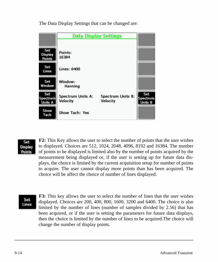
The Data Display Settings that can be changed are:
F2: This Key allows the user to select the number of points that the user wishesto displayed. Choices are 512, 1024, 2048, 4096, 8192 and 16384. The numberof points to be displayed is limited also by the number of points acquired by themeasurement being displayed or, if the user is setting up for future data dis-plays, the choice is limited by the current acquisition setup for number of pointsto acquire. The user cannot display more points than has been acquired. Thechoice will be affect the choice of number of lines displayed.
F3: This key allows the user to select the number of lines that the user wishesdisplayed. Choices are 200, 400, 800, 1600, 3200 and 6400. The choice is alsolimited by the number of lines (number of samples divided by 2.56) that hasbeen acquired, or if the user is setting the parameters for future data displays,then the choice is limited by the number of lines to be acquired.The choice willchange the number of display points.
9-14 Advanced Transient

F4: The window option is used to apply a shaping function to the waveform sig-nal before computing the FFT spectrum. The Hanning windows shapingsmooths out end effects and reduce leakage in the spectrum, and therefore rec-ommended for normal analyzer operation. The uniform window option does notapply any shaping and is subject to leakage and amplitude errors. This windowcan be used when analyzing transient signals that are completely containedwithin the analysis time record length.
F5: This parameter specifies the units for the analyzer spectrum only. Thechoices are: Acceleration, Velocity or Displacement. If the data was convertedto Velocity units on acquisition, then the only choices are velocity and displace-ment. If the data was converted to Displacement Units on acquisition, then thereis no choice, Displacement Units must be used.
F6: This feature may be enabled only when Tachometer data has been acquired.It will cause dotted lines to be overlaid on the waveform display showing thelocation of the tachometer pulses. Tach lines are not available for the full tran-sient waveform view.
F11: This parameter specifies the units for the analyzer spectrum only. Thechoices are: Acceleration, Velocity or Displacement. If the data was convertedto Velocity units on acquisition, then the only choices are velocity and displace-ment. If the data was converted to Displacement Units on acquisition, then thereis no choice, Displacement Units must be used.
F2: When a full transient waveform plot is displayed, a section of waveformtime represented by two solid vertical lines is superimposed onto the displayedplot. Pressing the Scroll Left and Scroll Right keys will move the selected sec-tion of the transient waveform left/right by 512 points (200 lines). The wave-form and spectrum will be updated with the data contained in the new selectedsection.
F3: When a full transient waveform plot is displayed, a section of waveformtime represented by two solid vertical lines is superimposed onto the displayed
9-15

plot. Pressing the Scroll Left and Scroll Right keys will move the selected sec-tion of the transient waveform left/right by 512 points (200 lines). The wave-form and spectrum will be updated with the data contained in the new selectedsection.
F4: Displays the plot for the entire screen. The Up, Down, Left and Right arrowkeys will work for the active plot. Pressing any of the lower soft keys or theGoBack key will cause the plot display to go back to its normal size and the softkeys will be visible.
F5: Switches the active plot between the plots visible on the screen. A box willbe drawn around the active plot. All key functions will apply to the active plot
F6: For most applications, if there are more than two plots available, this keywill start the Select Plot screen that will set which plot or plots will be dis-played. The format for displaying multiple plots can also be set. If there are onlytwo plots available, this key will toggle between a dual plot and the two individ-ual plots.
9-16 Advanced Transient
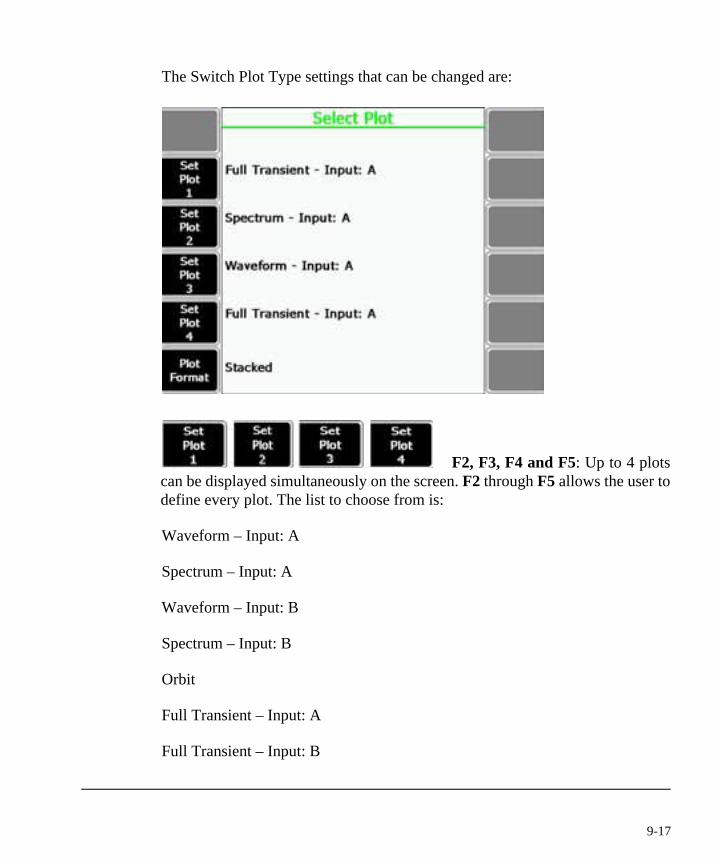
The Switch Plot Type settings that can be changed are:
F2, F3, F4 and F5: Up to 4 plotscan be displayed simultaneously on the screen. F2 through F5 allows the user todefine every plot. The list to choose from is:
Waveform – Input: A
Spectrum – Input: A
Waveform – Input: B
Spectrum – Input: B
Orbit
Full Transient – Input: A
Full Transient – Input: B
9-17

F6: This key sets the format for how multiple plots are displayed. The stackedformat is default and will show the plots with the width of the display area andstacked one on top of the others. The Quad format will show four plots in thequarters of the screen.
F7: This will print the current plot to the printing device.
F8: When a full transient waveform plot is displayed, a section of waveformtime represented by two solid vertical lines is superimposed onto the displayedplot. The width of the section depends on the number of points and number oflines defined under the Display Settings function. Pressing the Page Left andPage Right key will move the selected section of the transient waveform left/right by the number of points.
F9: When a full transient waveform plot is displayed, a section of waveformtime represented by two solid vertical lines is superimposed onto the displayedplot. The width of the section depends on the number of points and number oflines defined under the Display Settings function. Pressing the Page Left andPage Right key will move the selected section of the transient waveform left/right by the number of points.
Example of Stacked Plot Format Example of Quad Plot Format
9-18 Advanced Transient
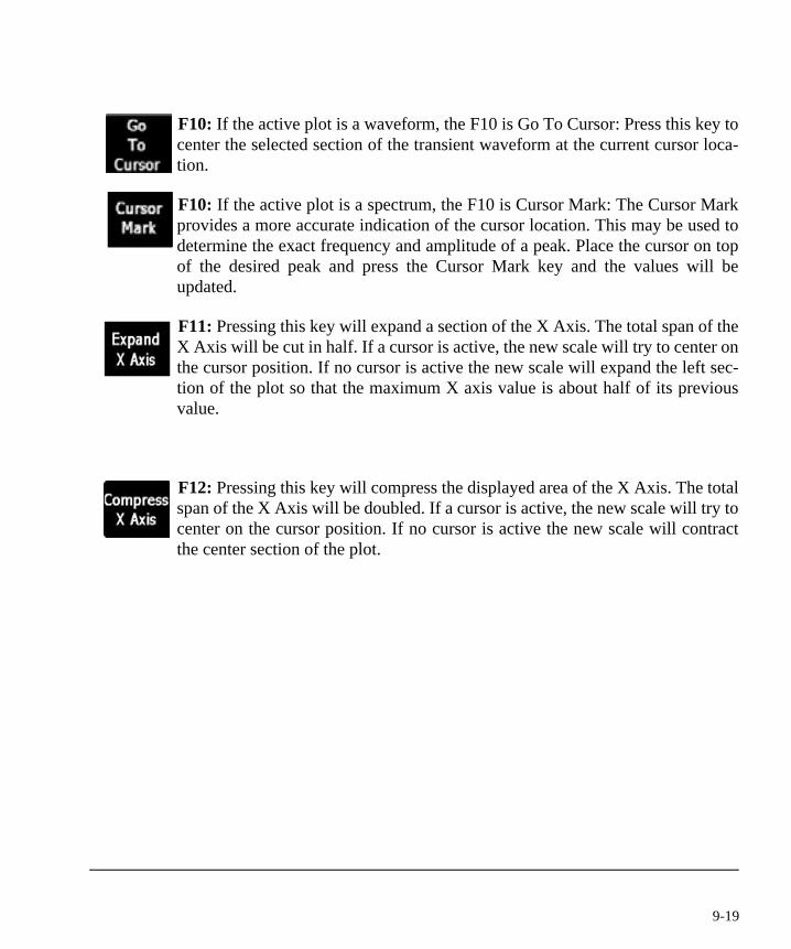
F10: If the active plot is a waveform, the F10 is Go To Cursor: Press this key tocenter the selected section of the transient waveform at the current cursor loca-tion.
F10: If the active plot is a spectrum, the F10 is Cursor Mark: The Cursor Markprovides a more accurate indication of the cursor location. This may be used todetermine the exact frequency and amplitude of a peak. Place the cursor on topof the desired peak and press the Cursor Mark key and the values will beupdated.
F11: Pressing this key will expand a section of the X Axis. The total span of theX Axis will be cut in half. If a cursor is active, the new scale will try to center onthe cursor position. If no cursor is active the new scale will expand the left sec-tion of the plot so that the maximum X axis value is about half of its previousvalue.
F12: Pressing this key will compress the displayed area of the X Axis. The totalspan of the X Axis will be doubled. If a cursor is active, the new scale will try tocenter on the cursor position. If no cursor is active the new scale will contractthe center section of the plot.
9-19
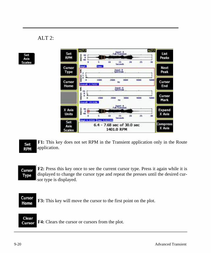
ALT 2:
F1: This key does not set RPM in the Transient application only in the Routeapplication.
F2: Press this key once to see the current cursor type. Press it again while it isdisplayed to change the cursor type and repeat the presses until the desired cur-sor type is displayed.
F3: This key will move the cursor to the first point on the plot.
F4: Clears the cursor or cursors from the plot.
9-20 Advanced Transient
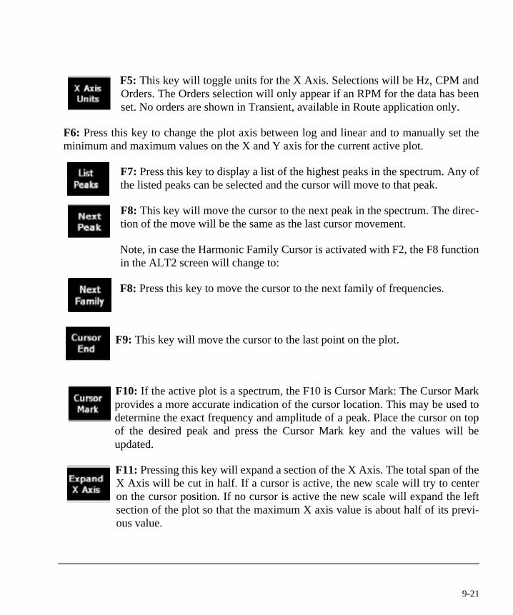
F5: This key will toggle units for the X Axis. Selections will be Hz, CPM andOrders. The Orders selection will only appear if an RPM for the data has beenset. No orders are shown in Transient, available in Route application only.
F6: Press this key to change the plot axis between log and linear and to manually set theminimum and maximum values on the X and Y axis for the current active plot.
F7: Press this key to display a list of the highest peaks in the spectrum. Any ofthe listed peaks can be selected and the cursor will move to that peak.
F8: This key will move the cursor to the next peak in the spectrum. The direc-tion of the move will be the same as the last cursor movement.
Note, in case the Harmonic Family Cursor is activated with F2, the F8 functionin the ALT2 screen will change to:
F8: Press this key to move the cursor to the next family of frequencies.
F9: This key will move the cursor to the last point on the plot.
F10: If the active plot is a spectrum, the F10 is Cursor Mark: The Cursor Markprovides a more accurate indication of the cursor location. This may be used todetermine the exact frequency and amplitude of a peak. Place the cursor on topof the desired peak and press the Cursor Mark key and the values will beupdated.
F11: Pressing this key will expand a section of the X Axis. The total span of theX Axis will be cut in half. If a cursor is active, the new scale will try to centeron the cursor position. If no cursor is active the new scale will expand the leftsection of the plot so that the maximum X axis value is about half of its previ-ous value.
9-21
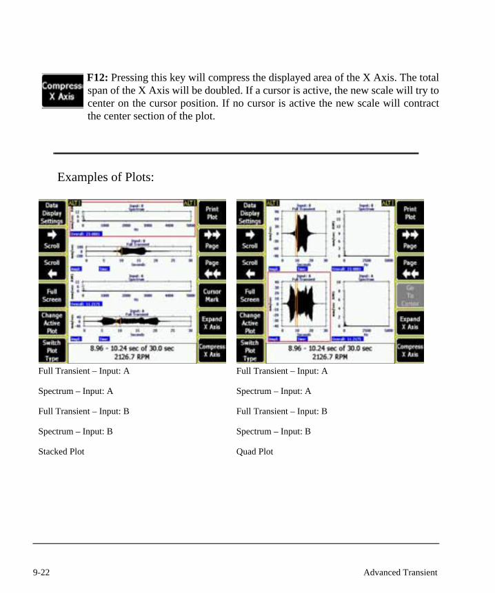
F12: Pressing this key will compress the displayed area of the X Axis. The totalspan of the X Axis will be doubled. If a cursor is active, the new scale will try tocenter on the cursor position. If no cursor is active the new scale will contractthe center section of the plot.
Examples of Plots:
Full Transient – Input: A
Spectrum – Input: A
Full Transient – Input: B
Spectrum – Input: B
Stacked Plot
Full Transient – Input: A
Spectrum – Input: A
Full Transient – Input: B
Spectrum – Input: B
Quad Plot
9-22 Advanced Transient

Full Transient – Input: A
Spectrum – Input: A
Waveform – Input: A
Stacked Plot
Full Transient – Input: A
Spectrum – Input: A
Waveform – Input: A
Quad Plot
Full Transient – Input: B
Spectrum – Input: B
Waveform – Input: B
Stacked Plot
Full Transient – Input: B
Spectrum – Input: B
Waveform – Input: B
Quad Plot
9-23

Full Transient – Input: A Full Transient – Input: B
Spectrum – Input: A Spectrum – Input: B
9-24 Advanced Transient

Waveform – Input: A Waveform – Input: A
Full Transient – Input: A
Full Transient – Input: B
Orbit
Stacked plot
Full Transient – Input: A
Full Transient – Input: B
Orbit
Quad plot
9-25

This overview is only a limited list with possible plots and is far from complete,but it should give a good overview of the possibilities.
Example (Case Study)
The Run up coast down from a fan was measured with 2 channels.
Channel A is measured in Horizontal direction.
Channel B is measured in Vertical direction.
The motor is frequency driven and the maximum speed is 2970 RPM.
The run up, steady state and coast down were measured in 3 minutes.
Orbit
9-26 Advanced Transient
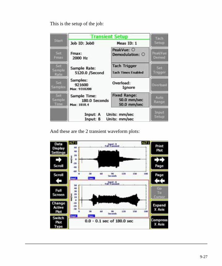
This is the setup of the job:
And these are the 2 transient waveform plots:
9-27

This is the Full transient Input B + spectrum and waveform during startup whenthe speed is 595 RPM.
9-28 Advanced Transient
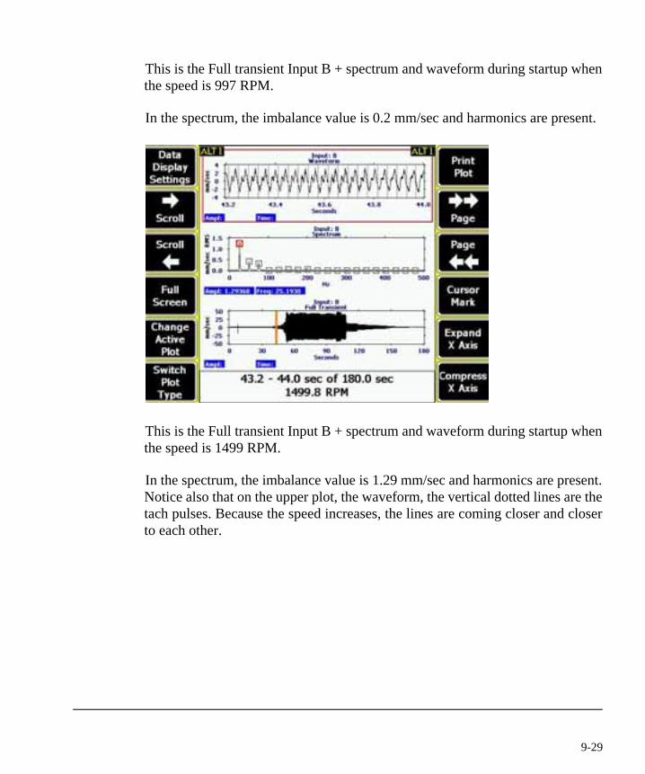
This is the Full transient Input B + spectrum and waveform during startup whenthe speed is 997 RPM.
In the spectrum, the imbalance value is 0.2 mm/sec and harmonics are present.
This is the Full transient Input B + spectrum and waveform during startup whenthe speed is 1499 RPM.
In the spectrum, the imbalance value is 1.29 mm/sec and harmonics are present.Notice also that on the upper plot, the waveform, the vertical dotted lines are thetach pulses. Because the speed increases, the lines are coming closer and closerto each other.
9-29
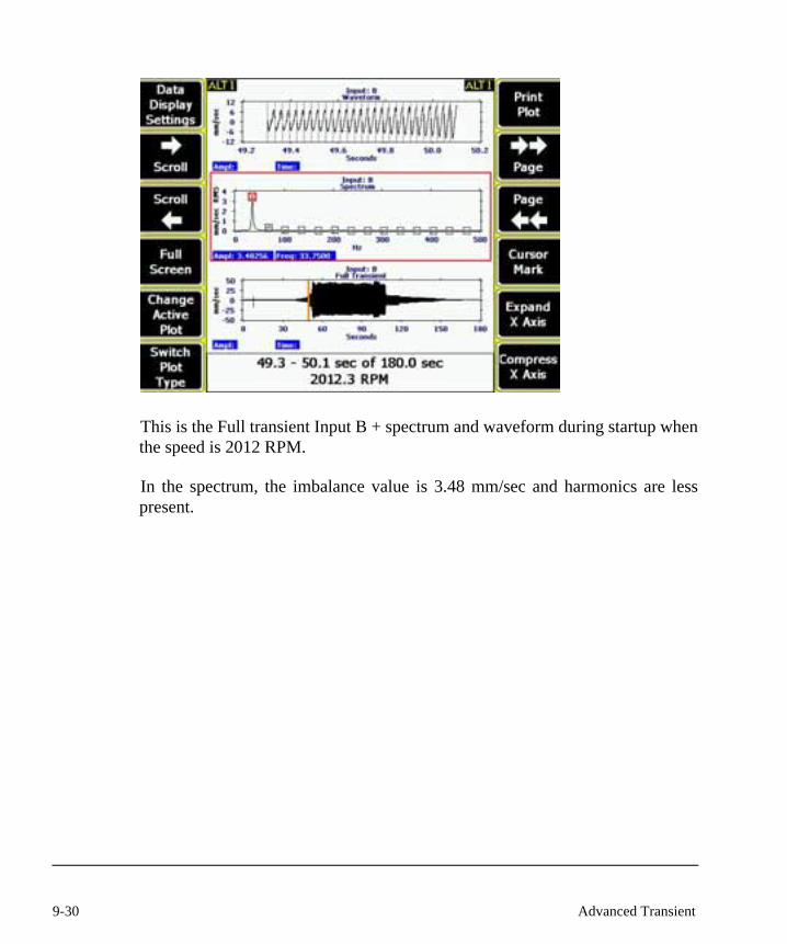
This is the Full transient Input B + spectrum and waveform during startup whenthe speed is 2012 RPM.
In the spectrum, the imbalance value is 3.48 mm/sec and harmonics are lesspresent.
9-30 Advanced Transient
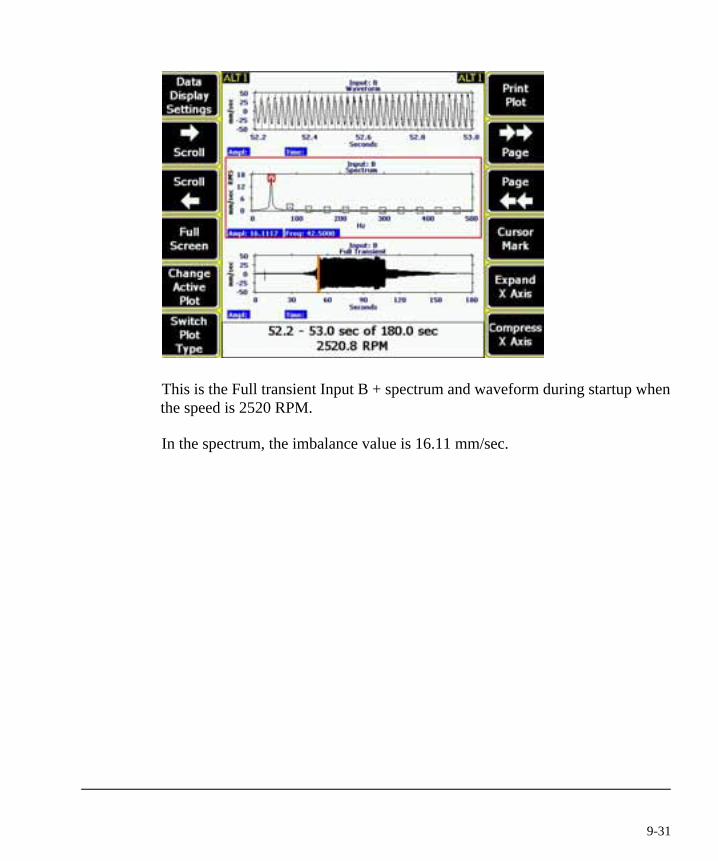
This is the Full transient Input B + spectrum and waveform during startup whenthe speed is 2520 RPM.
In the spectrum, the imbalance value is 16.11 mm/sec.
9-31

This is the Full transient Input B + spectrum and waveform during full speed.The speed is 2971 RPM.
In the spectrum, the imbalance value is 25.19 mm/sec.
9-32 Advanced Transient
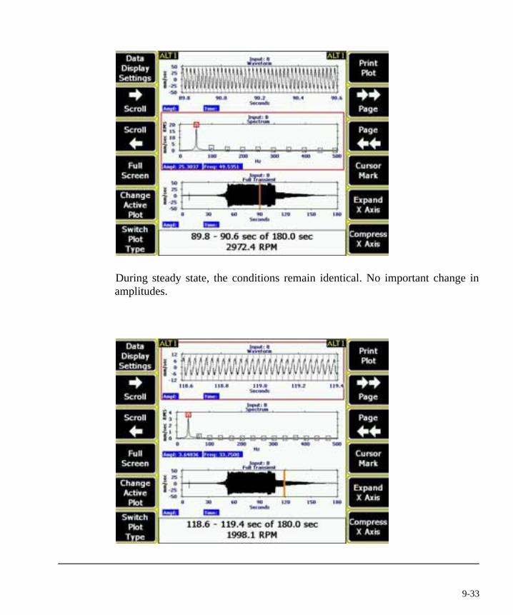
During steady state, the conditions remain identical. No important change inamplitudes.
9-33

This is the Full transient Input B + spectrum and waveform during Runout whenthe speed is 1998 RPM.
In the spectrum, the imbalance value is 3.64 mm/sec.
This is the Full transient Input B + spectrum and waveform during Runout whenthe speed is 1003 RPM.
In the spectrum, the imbalance value is 0.10 mm/sec.
Just like all job based data, the acquired information can be transferred into theAMS Machinery Health Manager for advanced analysis, reporting andarchiving.
9-34 Advanced Transient

The following plots are only a few examples of additional plots and tools insidethe Vibration Analysis software module that can be applied on data collectedwith the CSI 2130 Advanced Transient module.
Full Transient Input A Hz based Waterfall plot.
9-35

Order based colored Waterfall plot. A referenceand a primary cursor are installed.
Trend plot of all the energy between the referenceand the primary cursor in the waterfall plot.Because the waterfall plot was order based, and thereference cursor was just below 1 x RPM and theprimary cursor was just above 1 x RPM, this trendplot indicates the imbalance value during the tran-sient job.
During the start up, the critical speed is 1155 RPM.During the run out, the critical speed (imbalancevalue) is 1180 RPM
9-36 Advanced Transient

Full Transient Input A + colored waterfall plot. Hzbased
Full Transient Input B + colored waterfall plot. Hzbased
Full Transient Input A and B + unfiltered orbit at2974 RPM
Full Transient Input A and B + filtered orbit (1 xRPM BP) at 2974 RPM
9-37

Full Transient Input A + RPM plot + detailed spec-trum and waveform at 1669 RPM.
Full Transient Input B + RPM plot + detailed spec-trum and waveform at 2974 RPM.
Nyquist and Bode plot during start up. Amplitudesversus RPM
Nyquist and Bode plot during start up. Amplitudesversus Time.
9-38 Advanced Transient
Chapter 10
ODS Modal
What is an Operating Deflection Shape?The CSI 2130 ODS/Modal downloadable program provides a convenient user interface for acquiring ODS and Modal data. The data is formatted for use with ME'scope ODS/Modal analysis software. Data is uploaded through Data Transfer, viewed from Vibration Analysis and then exported to ME’Scoope software for analysis. The Advanced Cross-Channel program (part#A2130S3) is also included as part of this package.
Traditionally, an ODS has been defined as the deflection of a structure at a particular frequency. However, an ODS can be defined more generally as any forced motion of two or more points on a structure. Specifying the motion of two or more points defines a shape. Stated differently, a shape is the motion of one point relative to all others. Motion is a vector quantity, which means that it has location and direction associated with it. This is also called a Degree of Freedom, or DOF.
What is MODAL?
Modal Analysis is the process of determining the modal characteristics (nat-ural frequency, mode shape and damping) of an elastic structure. The utiliza-tion of the term “structure” in the definition For Modal Analysis does not imply that the method is limited to classical civil engineering structures such as bridges and buildings. It can be used to define the modal characteristic of any structure including mechanical equipment (fans, pumps, compressors, rolling mills, paper machines, computer components, etc.).
10-1

Hereinafter the term “structure” shall refer to the components of mechanical equipment as well as the structural framework supporting same.
All structures have at least one natural frequency. Most structures have many natural frequencies. Structures are very sensitive to dynamic forces that have a frequency at or near a natural frequency. The excitation of a natural fre-quency is commonly referred to as resonance. The magnitude of the fre-quency at which resonance will occur is dependent upon the distribution of mass (weight) and stiffness of a structure.
If a machine produces a force near the natural frequency of the structure, vibration levels will most probably be excessive. This can result in a less than optimal performance level of the equipment and can cause premature failure of structural and mechanical components of the machine due to fatigue.
The excitation of natural frequency is the most common reason for excessive vibrations in mechanical equipment. The source of vibration may be due to unbalance, misalignment, gear mesh, etc. However, in many cases, the response (vibration level) to these dynamic forces would be acceptable if a natural frequency was not excited. It is for this reason that Modal Analysis is one of the most important and powerful tools that a vibration analyst can employ.
Modal Analysis can be separated into two categories; Experimental Modal Analysis (EMA) and Finite Element Analysis (FEA).
10-2 ODS Modal
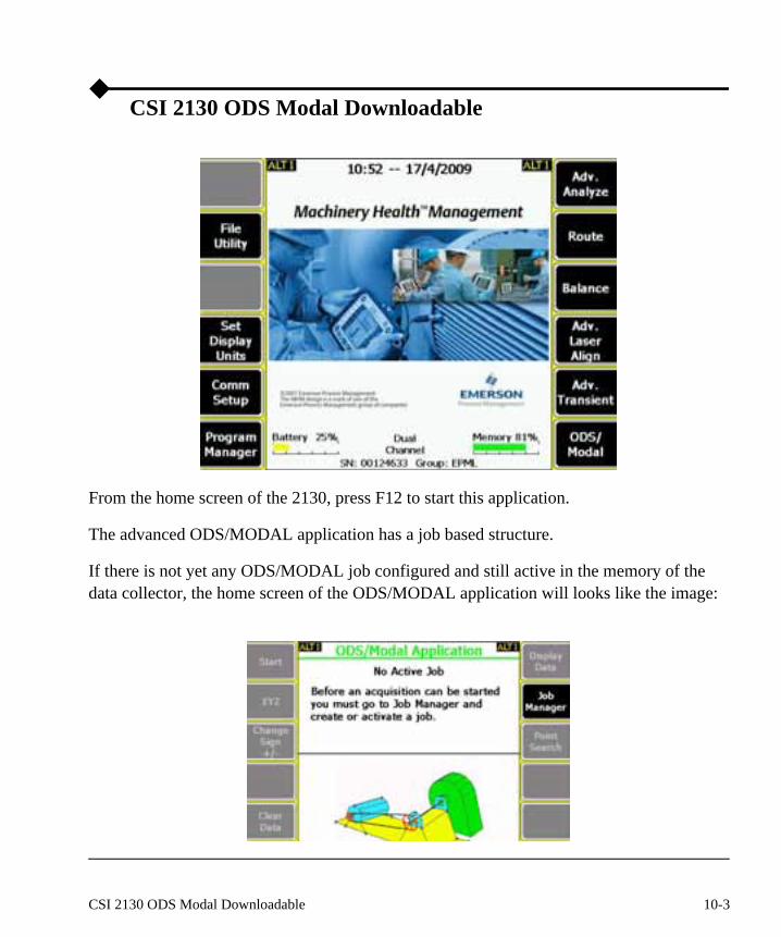
CSI 2130 ODS Modal Downloadable
From the home screen of the 2130, press F12 to start this application.
The advanced ODS/MODAL application has a job based structure.
If there is not yet any ODS/MODAL job configured and still active in the memory of the data collector, the home screen of the ODS/MODAL application will looks like the image:
10-3CSI 2130 ODS Modal Downloadable
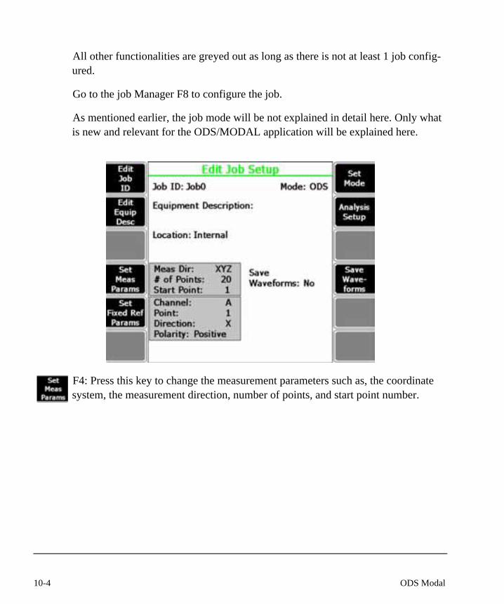
All other functionalities are greyed out as long as there is not at least 1 job config-ured.
Go to the job Manager F8 to configure the job.
As mentioned earlier, the job mode will be not explained in detail here. Only what is new and relevant for the ODS/MODAL application will be explained here.
F4: Press this key to change the measurement parameters such as, the coordinate system, the measurement direction, number of points, and start point number.
10-4 ODS Modal
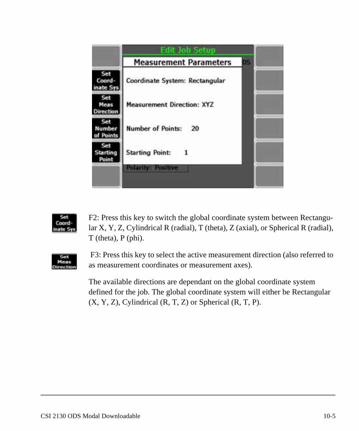
F2: Press this key to switch the global coordinate system between Rectangu-lar X, Y, Z, Cylindrical R (radial), T (theta), Z (axial), or Spherical R (radial), T (theta), P (phi).
F3: Press this key to select the active measurement direction (also referred to as measurement coordinates or measurement axes).
The available directions are dependant on the global coordinate system defined for the job. The global coordinate system will either be Rectangular (X, Y, Z), Cylindrical (R, T, Z) or Spherical (R, T, P).
10-5CSI 2130 ODS Modal Downloadable
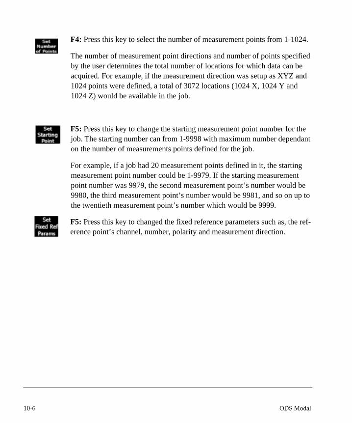
F4: Press this key to select the number of measurement points from 1-1024.
The number of measurement point directions and number of points specified by the user determines the total number of locations for which data can be acquired. For example, if the measurement direction was setup as XYZ and 1024 points were defined, a total of 3072 locations (1024 X, 1024 Y and 1024 Z) would be available in the job.
F5: Press this key to change the starting measurement point number for the job. The starting number can from 1-9998 with maximum number dependant on the number of measurements points defined for the job.
For example, if a job had 20 measurement points defined in it, the starting measurement point number could be 1-9979. If the starting measurement point number was 9979, the second measurement point’s number would be 9980, the third measurement point’s number would be 9981, and so on up to the twentieth measurement point’s number which would be 9999.
F5: Press this key to changed the fixed reference parameters such as, the ref-erence point’s channel, number, polarity and measurement direction.
10-6 ODS Modal
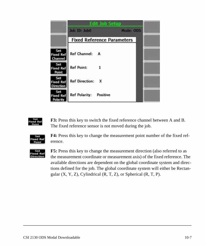
F3: Press this key to switch the fixed reference channel between A and B. The fixed reference sensor is not moved during the job.
F4: Press this key to change the measurement point number of the fixed ref-erence.
F5: Press this key to change the measurement direction (also referred to as the measurement coordinate or measurement axis) of the fixed reference. The available directions are dependent on the global coordinate system and direc-tions defined for the job. The global coordinate system will either be Rectan-gular (X, Y, Z), Cylindrical (R, T, Z), or Spherical (R, T, P).
10-7CSI 2130 ODS Modal Downloadable

F6: Press this key to change the measurement polarity of the fixed reference. The polarity can be either positive or negative.
The polarity of the measurement indicates the direction in which a measure-ment is to be made when data is acquired. The direction of the measurement is usually determined by the construction of the equipment data is being acquired on. In certain locations on the equipment it may not be possible to orient the sensor in the positive direction; therefore, a negative direction mea-surement must be specified.
F7: Press this key to switch the job mode between ODS and MODAL. When creating a new job or when editing an existing job with no data stored, this key is used to set up the operating mode and appropriate values for the job. Once any data is stored in the job, the job’s mode of operation can not be modified.
When this key is selected, a warning message is displayed. If it is desired to continue and change the existing setup, choose YES by pressing the Enter key. If it is not desired to continue and change the existing setup, choose No by pressing the Back key. Since some of the options are different between the two modes, the last setup specified for a mode is restored when using this key to switch between modes.
10-8 ODS Modal
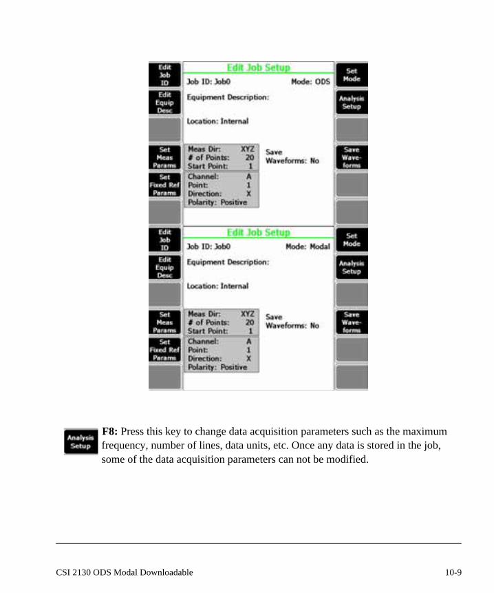
F8: Press this key to change data acquisition parameters such as the maximum frequency, number of lines, data units, etc. Once any data is stored in the job, some of the data acquisition parameters can not be modified.
10-9CSI 2130 ODS Modal Downloadable
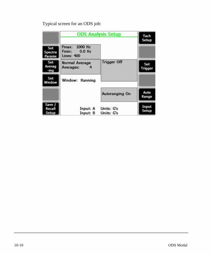
Typical screen for an ODS job:
10-10 ODS Modal
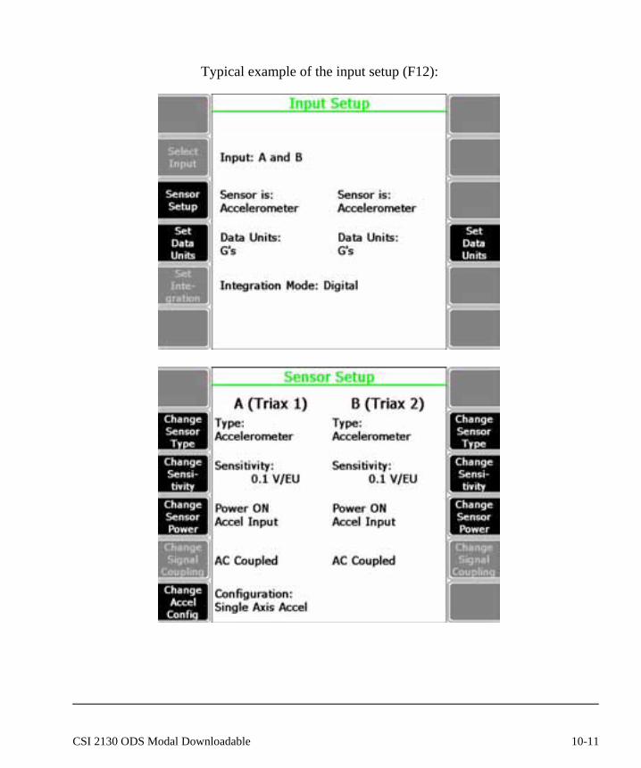
Typical example of the input setup (F12):
10-11CSI 2130 ODS Modal Downloadable
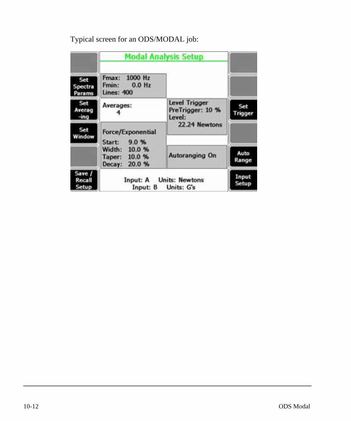
Typical screen for an ODS/MODAL job:
10-12 ODS Modal

Typical example of the input setup (F12):
10-13CSI 2130 ODS Modal Downloadable

F10: Press this key to switch between saving and not saving waveform data with the ODS/Modal data. The time waveforms are not required for ODS/MODAL jobs, but may be stored for reference.
After configuring a job, the home screen of the ODS/MODAL application will look like:
10-14 ODS Modal
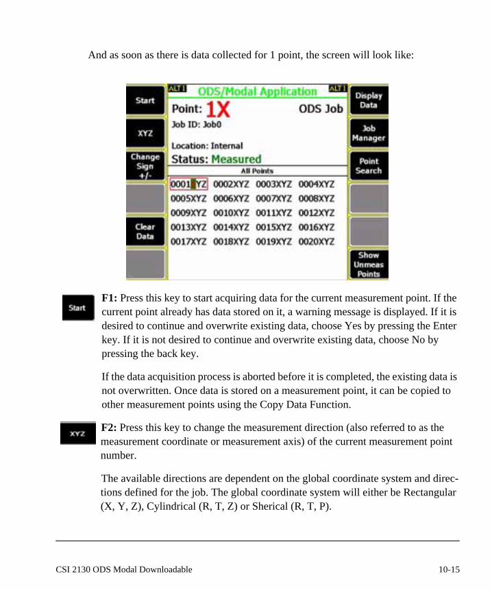
And as soon as there is data collected for 1 point, the screen will look like:
F1: Press this key to start acquiring data for the current measurement point. If the current point already has data stored on it, a warning message is displayed. If it is desired to continue and overwrite existing data, choose Yes by pressing the Enter key. If it is not desired to continue and overwrite existing data, choose No by pressing the back key.
If the data acquisition process is aborted before it is completed, the existing data is not overwritten. Once data is stored on a measurement point, it can be copied to other measurement points using the Copy Data Function.
F2: Press this key to change the measurement direction (also referred to as the measurement coordinate or measurement axis) of the current measurement point number.
The available directions are dependent on the global coordinate system and direc-tions defined for the job. The global coordinate system will either be Rectangular (X, Y, Z), Cylindrical (R, T, Z) or Sherical (R, T, P).
10-15CSI 2130 ODS Modal Downloadable

F3: Press this key to change the polarity of the current measurement point between positive (no sign displayed) and negative (-).
The polarity of the measurement indicates the direction in which a measurement is to be made when data is acquired. The direction of the measurement is usu-ally determined by the construction of the equipment data is being acquired on. In certain locations on the equipment it may not be possible to orient the sensor in the positive direction; therefore, a negative direction measurement must be specified.
A measurement point’s polarity can be changed after data has been acquired and stored for that measurement point.
F5: Press this key to clear the data from the current measurement point.
A warning message is displayed before any data is cleared. If clearing the selected data is desired, choose Yes by pressing the Enter key. If clearing the selected data is not desired, choose No by pressing the Back key.
Caution!Use extreme caution when using the Clear Data function when the analyzer contains important collected data. After answering Yes, the data can not be retrieved.
F7: Press this key to display the data for the current measurement point.
F8: Press this key to create a new job, edit an existing job, activate a job, or transfer a job to the host computer.
F9: Press this key to change the current measurement point by specifying a new point number and direction.
From the Point Search screen, use the number keys to enter a new number. Use the Up and Down Arrow keys to select the measurement direction. The Delete Digit key deletes the digit to the left of the cursor. The Clear Number key clears the entire number. The Back key reloads the original number.
10-16 ODS Modal
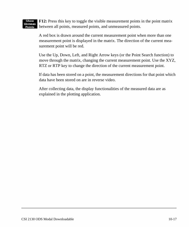
F12: Press this key to toggle the visible measurement points in the point matrix between all points, measured points, and unmeasured points.
A red box is drawn around the current measurement point when more than one measurement point is displayed in the matrix. The direction of the current mea-surement point will be red.
Use the Up, Down, Left, and Right Arrow keys (or the Point Search function) to move through the matrix, changing the current measurement point. Use the XYZ, RTZ or RTP key to change the direction of the current measurement point.
If data has been stored on a point, the measurement directions for that point which data have been stored on are in reverse video.
After collecting data, the display functionalities of the measured data are as explained in the plotting application.
10-17CSI 2130 ODS Modal Downloadable

10-18 ODS Modal
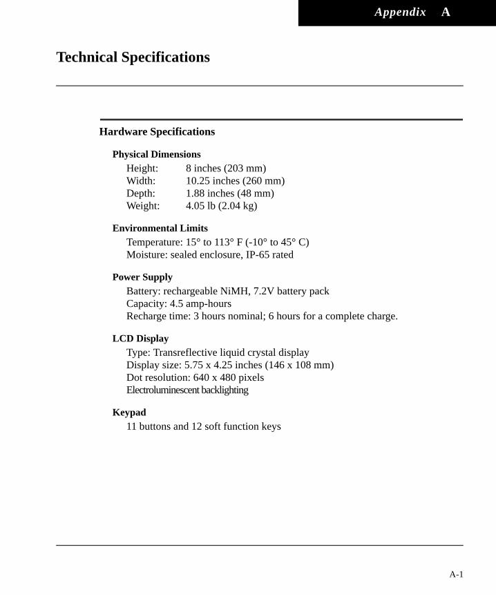
Appendix A
Technical Specifications
Hardware Specifications
Physical DimensionsHeight: 8 inches (203 mm)Width: 10.25 inches (260 mm)Depth: 1.88 inches (48 mm)Weight: 4.05 lb (2.04 kg)
Environmental LimitsTemperature: 15° to 113° F (-10° to 45° C) Moisture: sealed enclosure, IP-65 rated
Power SupplyBattery: rechargeable NiMH, 7.2V battery packCapacity: 4.5 amp-hours Recharge time: 3 hours nominal; 6 hours for a complete charge.
LCD DisplayType: Transreflective liquid crystal displayDisplay size: 5.75 x 4.25 inches (146 x 108 mm)Dot resolution: 640 x 480 pixelsElectroluminescent backlighting
Keypad11 buttons and 12 soft function keys
A-1
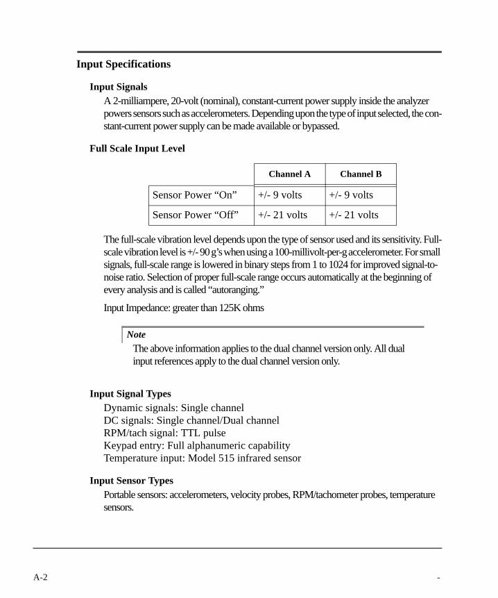
Input Specifications
Input SignalsA 2-milliampere, 20-volt (nominal), constant-current power supply inside the analyzer powers sensors such as accelerometers. Depending upon the type of input selected, the con-stant-current power supply can be made available or bypassed.
Full Scale Input Level
The full-scale vibration level depends upon the type of sensor used and its sensitivity. Full-scale vibration level is +/- 90 g’s when using a 100-millivolt-per-g accelerometer. For small signals, full-scale range is lowered in binary steps from 1 to 1024 for improved signal-to-noise ratio. Selection of proper full-scale range occurs automatically at the beginning of every analysis and is called “autoranging.”
Input Impedance: greater than 125K ohms
NoteThe above information applies to the dual channel version only. All dual input references apply to the dual channel version only.
Input Signal TypesDynamic signals: Single channel DC signals: Single channel/Dual channelRPM/tach signal: TTL pulseKeypad entry: Full alphanumeric capabilityTemperature input: Model 515 infrared sensor
Input Sensor TypesPortable sensors: accelerometers, velocity probes, RPM/tachometer probes, temperature sensors.
Channel A Channel B
Sensor Power “On” +/- 9 volts +/- 9 volts
Sensor Power “Off” +/- 21 volts +/- 21 volts
A-2 -

Installed sensors: Any vibration or dynamic sensor with a voltage output; any DC-type signal.
Input Unit Types
The CSI 2130 calculates the integration or differentiation necessary to convert from sensor units to other units for display purposes. The CSI 2130 uses analog integration circuitry for conversions from acceleration to velocity or displacement.
Tachometer InputThe tachometer input measures a once-per-rev pulse. This capability lets the analyzer mea-sure RPM and synchronous vibration and phase.
RPM range: 6 to 100,000 RPMTach input level: TTL input, built in conditioning for non-TTL signals, adjustable trigger.
Pseudo TachGenerates tach pulses for hidden shafts.
Triaxial Sensor InputInternal multiplexer for automatic sequencing of triaxial measurements.
AutorangingThe CSI 2130 automatically scans the input signal for each measurement. The analyzer sets the input range to maximize the dynamic resolution.
Demodulator and PeakVueBuilt-in demodulator and PeakVue function, with selectable filters.
Vibration Signals Units
Acceleration g’s
Velocity In./sec or mm/sec
Displacement Mils or microns
Other dynamic signals Any user-specified unit
DC Signals Any user-specified unit
A-3
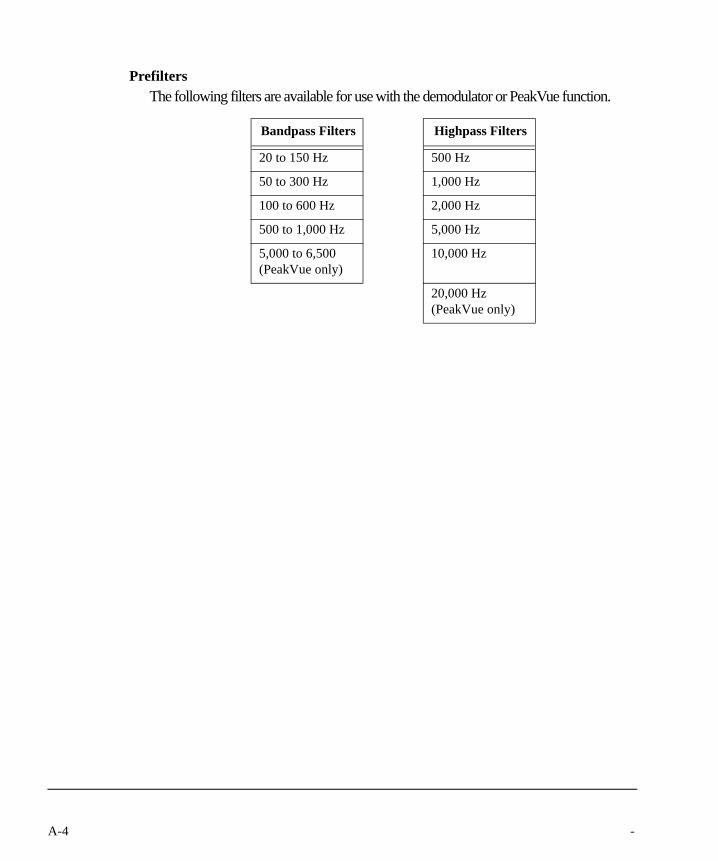
PrefiltersThe following filters are available for use with the demodulator or PeakVue function.
Bandpass Filters Highpass Filters
20 to 150 Hz 500 Hz
50 to 300 Hz 1,000 Hz
100 to 600 Hz 2,000 Hz
500 to 1,000 Hz 5,000 Hz
5,000 to 6,500 (PeakVue only)
10,000 Hz
20,000 Hz (PeakVue only)
A-4 -

Measurement Specifications
Frequency AnalysisA/D converter: 16 bits of accuracy.Dynamic range: Converter has 96 dB range. (Coupled with analog integration this provides better than 120dB for typical applications.)Averaging modes: normal, exponential, peak hold, order tracking, negative averaging, synchronous timeNumber of averages: 5,000 in Route mode, 10,000 in Job mode.Resolution: 1/3 Octave, 100, 200, 400, 800, 1600, 3200, 6400, or 12800 lines of resolution. True Zoom provides effective resolution of up to 300,000 lines.Frequency range: DC to 10 Hz minimum
DC to 80 kHz maximumResponse: flat to DC for non-integrated and DC-coupled signals;
optional AC coupling -3 dB at 1 HzFrequency Units: Hz, CPM, Orders.Automatic Integrator Correction feature allows precise measurement of low fre-quency vibrations down to 0.2 Hz.Full-scale range: 3mV to 21V.Noise floor: typically less than 0.2 µV for a 400-line spectrum at 1000 Hz
maximum frequency.Windows: Hanning or uniform.Integration: None, Single, Double (Analog or Digital).
CursorSpectrum Single, Harmonic, Moving Harmonic, Sideband, and Time/Frequency for waveform.
ScalingLinear or Log, both X and Y.
Data Storage CapacityCSI 2130 with PCMCIA Slot(s) Internal memory: 32 MB for programs and data storage.External memory: memory expandable with off the shelf ATA and Compact Flash RAM cards.
A-5

CSI 2130 with Ethernet port and SD SlotInternal memory: 256 MB for programs and data storage.External memory: memory expandable with off the shelf SD Flash and RAM cards.
Number of Stored SpectraCan store 1,000 400-line spectra for each MB of memory. Generally, with spectra, wave-form, and trend parameters, 1 MB is sufficient for 200 to 300 measurement points.
Data Analysis Speed400 line / 1000 HZ spectrum / 67% overlap: 7 avg/sec
1600 line / 1000 Hz spectrum / 67% overlap: 2 avg/sec
A-6 -

Output
Communications with Host computerThese communication outputs include USB, Ethernet, Serial, E-mailable data files. To use a USB, computer must have a USB port and run Windows 2000, XP, or Windows VISTA. To use Ethernet, a card and cable must be inserted into the analyzer. To use Serial commu-nications, the computer must have an RS232 serial link. Baud rates may be selected between 57.6K and 115.2K.
A-7

A-8 -
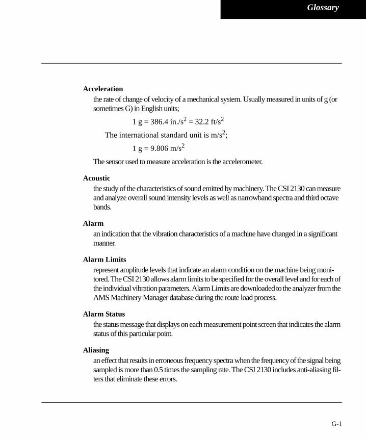
Glossary
Accelerationthe rate of change of velocity of a mechanical system. Usually measured in units of g (or sometimes G) in English units;
1 g = 386.4 in./s2 = 32.2 ft/s2
The international standard unit is m/s2;
1 g = 9.806 m/s2
The sensor used to measure acceleration is the accelerometer.
Acousticthe study of the characteristics of sound emitted by machinery. The CSI 2130 can measure and analyze overall sound intensity levels as well as narrowband spectra and third octave bands.
Alarman indication that the vibration characteristics of a machine have changed in a significant manner.
Alarm Limits represent amplitude levels that indicate an alarm condition on the machine being moni-tored. The CSI 2130 allows alarm limits to be specified for the overall level and for each of the individual vibration parameters. Alarm Limits are downloaded to the analyzer from the AMS Machinery Manager database during the route load process.
Alarm Status the status message that displays on each measurement point screen that indicates the alarm status of this particular point.
Aliasingan effect that results in erroneous frequency spectra when the frequency of the signal being sampled is more than 0.5 times the sampling rate. The CSI 2130 includes anti-aliasing fil-ters that eliminate these errors.
G-1
Amplitudethe magnitude (RMS, peak, peak-to-peak, average, or dc) of a measured signal.
Analog Integrationa method of converting from acceleration to the equivalent velocity signal or converting a velocity signal to the equivalent displacement signal. Analog integration is superior to the equivalent digital method as it produces much less low-frequency components in the vibra-tion spectrum.
Analysis Parametersdivides the frequency spectrum into bands that are individually measured and analyzed.
Analysis Parameter Setsincludes up to 12 individual analysis parameters, and also contains instructions that tell the machinery analyzer how to acquire data.
Autorangingthe process of automatically adjusting the input gain of an analyzer to match the amplitude of a signal. Optimizes the use of the dynamic range of the analyzer and improves signal-to-noise ratio.
Averaginga method of collecting data where the spectra are averaged together to eliminate random noise.
A-Weightinga frequency spectrum shaping that is applied to frequency spectra in acoustics. The effect is designed to approximate the way that the human ear perceives the loudness of sound. Sound levels are reduced at low frequencies and at very high frequencies where the ear is less sensitive. There are national and international standards for A-weighting.
Bandwidth the analysis frequency range over which data will be collected. For normal route measure-ments, this is listed by the “BW =” parameter located on the screen display. It can be spec-ified as a frequency range in Hz, as an order-based analysis (for example 10xRPM), or in CPM.
G-2

Baud Rateunit of speed for data transmission over a serial communications link. The CSI 2130 sup-ports baud rates from 57.6K and 115.2K baud.
Bode Plota graphic plot that shows how the 1xRPM amplitude and phase have varied with the RPM of a machine. These are always measured over a startup or coastdown of a machine and are used to identify shaft resonances and other signal characteristics.
CoherenceA function of frequency which describes the degree of linear relationship between two sig-nals. Used to assess cross-channel measurement quality, locate noise sources, and to check out transmission paths.
CPMcycles per minute. Favored by many in machine vibration analysis because the vibration caused by unbalance shows up at a frequency in CPM equal to the RPM of the shaft. 60 cycles per minute (CPM) is equivalent to one (1) cycle per second which equals one (1) hertz.
Crest Factorthe ratio of peak to RMS levels of a signal. A single-frequency signal has a crest factor of 1.414; random noise has a crest factor of approximately 3; signals with impulsive content have higher crest factor values. The crest factor can be used to check for impacting, such as caused by rolling bearing defects.
Cursora manually controlled marker that can be moved across the plot display indicating fre-quency and amplitude at the cursor location.
Decibels (dB)a logarithmic system of non-dimensional units that measures the size of a quantity relative to a reference level. Any quantity can be measured in this way, as can any two quantities with the same dimensions be compared using decibel measure.
Given a reference power (amplitude squared) level Wref, any other power quantity W, having the same dimensions, may be expressed in decibels using the formula:
1
dB = 10log10W
Wref
G-3
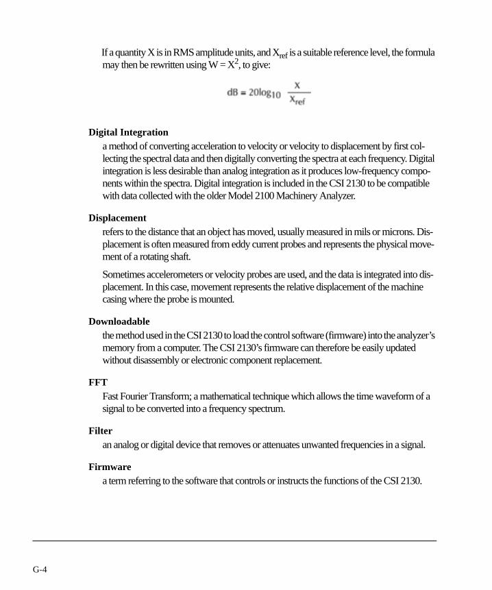
If a quantity X is in RMS amplitude units, and Xref is a suitable reference level, the formula may then be rewritten using W = X2, to give:
2
Digital Integrationa method of converting acceleration to velocity or velocity to displacement by first col-lecting the spectral data and then digitally converting the spectra at each frequency. Digital integration is less desirable than analog integration as it produces low-frequency compo-nents within the spectra. Digital integration is included in the CSI 2130 to be compatible with data collected with the older Model 2100 Machinery Analyzer.
Displacementrefers to the distance that an object has moved, usually measured in mils or microns. Dis-placement is often measured from eddy current probes and represents the physical move-ment of a rotating shaft.
Sometimes accelerometers or velocity probes are used, and the data is integrated into dis-placement. In this case, movement represents the relative displacement of the machine casing where the probe is mounted.
Downloadablethe method used in the CSI 2130 to load the control software (firmware) into the analyzer’s memory from a computer. The CSI 2130’s firmware can therefore be easily updated without disassembly or electronic component replacement.
FFTFast Fourier Transform; a mathematical technique which allows the time waveform of a signal to be converted into a frequency spectrum.
Filteran analog or digital device that removes or attenuates unwanted frequencies in a signal.
Firmwarea term referring to the software that controls or instructs the functions of the CSI 2130.
dB = 20log10X
Xref
G-4
Frequencynumber of times an “event” repeats in a specific period of time. Units are hertz (Hz equals cycles per second) or CPM (cycles per minute).
Fundamentalprimary frequency of rotation for a machine (1xRPM); usually causes the highest peak of energy in the spectrum.
Fundamental Frequencya peak selected as the basis from which harmonic peaks are marked.
g’s a unit of acceleration, commonly used with the English system of units; One (1) g repre-sents the acceleration due to gravity at sea level and is approximately equal to 386.4 in./s2, or 32.2 ft/s2 (9.806 m/s2).
Hanninga shaping function applied to a time record before the FFT is calculated in order to smooth out end effects and reduce leakage in the spectrum. Usually the default window type to use when analyzing continuous signals because of the compromise between frequency dis-crimination and leakage suppression.
Harmonican integer multiple of a fundamental frequency.
Harmonic Marker a marker that appears on a spectral display to indicate the harmonic peaks of a fundamental peak.
Hertz a unit of frequency equal to cycles per second (CPS), usually abbreviated as Hz. One (1) hertz is equivalent to one (1) cycle per second, which equals 60 cycles per minute (CPM).
HFD high-frequency detection; the amplitude of vibration in g’s over a broad frequency band from 5 kHz up to 20 kHz or greater.
G-5

ICMInfluence Coefficient Method; the method used by the analyzer to calculate balancing solu-tions.
Impact Testa type of test used to investigate the properties of a structure, in which the structure is caused to vibrate by an impulsive load from an instrumented hammer, and the vibratory response is picked up by a vibration transducer.
Integrator see Signal Integration Mode.
Linesthe number of lines of resolution used for the spectrum calculation. Resolution (in Hz) equals maximum frequency divided by the number of Lines.
Live-timea feature that allows the CSI 2130 to dynamically display the spectrum (or waveform) during data collection.
Measurement Pointany location or point on a machine where measurements are made.
Mil(s)a unit of measure for displacement (thousandths of an inch).
Modema device that enables remote communications between the host computer and the analyzer over telephone lines.
Multiplane Balancing a method of balancing a machine that allows the measurement of the imbalance at several planes along the shaft of the machine. Correction weights are then added in each of these planes. Multiplane Balancing, as opposed to single plane balancing, is usually required when a machine has several rotating elements, such as flywheels, tightly coupled on a shaft and closely spaced.
G-6
Notesspecific observations that can be stored on the measurement point of a machine along with the collected data. These observations can be predefined notes from the AMS Machinery Manager database, user-defined notes that have been created via the analyzer's keypad, or a combination of the two methods.
Nyquist Plota polar plot of the peak amplitude and phase of the 1xRPM vibration component across a change in machine speeds. The Nyquist plot is typically used during startup or coastdown analysis to identify shaft resonances.
1/3-Octavemethod of measuring a signal by measuring the signal levels within a set of bandpass filters that have a bandwidth of 1/3 octave.
Order Tracking a measurement of a signal from a machine whose speed is changing with time, showing the level of one or more orders as a function of machine speed or time.
Overlapa function that speeds up data collection at low frequencies. The definable range of overlap for the CSI 2130 is 0 to 99% with 67% being the recommended value.
Peakthe largest signal level seen in a waveform over a period of time. For sinusoidal signals, the peak signal level is always 1.414 times the RMS value of the signal level. For non-sinu-soidal signals, the peak level is often larger than the result that this formula would produce.
Peak-to-Peakthe difference between the maximum and the minimum levels (positive or negative) in a signal over a given period of time. For a sinusoidal (single frequency) signal, the peak-to-peak level is always two times the peak level and 2.828 ( ) times the RMS level. For non-sinusoidal (multiple frequency) signals this is no longer true and there is no simple rela-tionship between peak-peak, peak, and RMS levels.
Period the time required for one complete cycle of a periodic signal.
2 2
G-7

Phase1xRPM phase represents the location of the shaft of a machine in degrees (0 to 360) with respect to the tachometer pulse where the largest vibration occurs.
Plane designates one or more of the rotating elements of a machine that is to be balanced. Each plane lies perpendicular to the line that defines the axis of rotation.
Pointany location on a machine where measurements are required; used interchangeably with measurement point.
Pre-Trigger triggered data acquisition using a delay such that the time record starts before the trigger event.
Data Transfer AMS Machinery Manager’s communications program that enables the host computer to transfer routes and data to and from the analyzer.
Real-TimeFFT frequency spectrum of an analog signal displayed instantaneously and continuously.
Resolutionthe frequency range represented by one line of an FFT spectrum. Found by dividing the maximum analysis frequency by the number of lines. The resolution in Hz is equal to the inverse of the data record length in seconds.
RMSroot mean square. When applied to a dynamic signal such as vibration or sound, refers to an averaged level of a function obtained by averaging the square of the signal level over a period of time (or number of data records), then taking the square root of the result.
Routeone or more machines and their respective measurement points organized in an efficient sequence for data collection.
G-8
Sidebanda frequency component that represents the effect of modulation on a signal. If a modulated signal has more than one component, each component will show sidebands. A sideband is spaced off from the frequency of the modulated signal by an amount equal to the modu-lating frequency. If the modulating signal has multiple components or if there is frequency modulation, the sideband pattern may be very complicated including sum and difference frequencies between the sideband component frequencies (intermodulation effects).
Signal Integration Mode provides a choice of analog or digital modes for the integration of signals. See also Analog Integration and Digital Integration.
Spectrumthe frequency domain representation of a signal. In practical measurements, the spectrum is usually displayed as a plot of magnitude verses frequency over a limited frequency range.
Station a grouping of machines within a company or a plant for the purpose of predictive mainte-nance; may include the entire facility or a logical division thereof; can then be subdivided into routes of machines for data collection.
Subharmonicsvibration frequencies which are integer fractions of the running speed (example 1/2 RPM, 1/3 RPM, etc.) or some other fundamental frequency.
Tachometera device that generates a pulse signal corresponding to the revolution of a shaft; used to measure turning speed. A single pulse per revolution may be used to trigger data acquisition synchronously with shaft rotation.
Transienta non-steady-state signal of brief duration; often refers to a startup or coastdown of a machine.
Trendplotting a number of measurements of a parameter over time.
G-9
Trigger causes the machinery analyzer to start data collection upon the receipt of a specified dynamic signal from a sensor or a pulse from a tachometer.
Uniform Window analyzing a signal without shaping; no window is applied. Sometimes used for collection of non-steady-state data.
Velocity the rate of change of displacement of a mechanical system. Units are inches per second (in/s or ips) in English units and m/s, cm/s, or mm/s in SI units. Can be measured directly with a velocity sensor or by integrating an acceleration signal from an accelerometer.
Vibration Parameters(also individual analysis parameters) up to twelve frequency band-limited parameters that are measured from the vibration signal. These parameters are defined in the analysis param-eter set and are loaded into the machinery analyzer for each point from the AMS Machinery Manager database.
Waveformanalog or digital representation of a signal or function displayed as amplitude vs. time.
Window see Hanning Window and Uniform Window.
G-10

Index
AAccel
set acceleration 2-11Accessories 1-5
Optional 1-5Typical sensor package 1-5
Advanced Analyze 8-1Advanced Cross Channel 8-13
Advanced Analyze 8-13Analyze Setup 8-14Input Setup 8-15Sensor Setup 8-15
ALT Screen 2-36Analysis Experts 6-1
Bump TestEquipment Off 6-6Equipment Running 6-7
Coast DownPeak and Phase 6-8Peak Hold 6-8
Cross Channel Amplitude/Phase 6-13High Frequency 6-2High Resolution 6-2Laser Speed Detection 6-5Low Frequency
Slow Speed Technology 6-4Orbit Plot 6-12Order Tracking 6-10Peakvue
Bearing/Gear 6-3Rotor Bar Test Motor Current 6-9selecting 6-1Synchronous 6-10Turning Speed Detection 6-5
Analyze 7-1Advanced 8-1Manual Analyze 7-2Special Features 7-11
Analyze Modeset 7-10
Autorange 7-15Averaging 7-20Aweighting 7-21
BBacklight
set backlight 2-41set backlight time 2-40
Base Firmwareupdating 2-29
battery packchanging 1-28recharging 1-27use and care 1-18
Baud Rateset baud rate 2-15
Bearing/Gear Analysis - PeakVue 6-3Beeper
set keypad beeper 2-38set status beeper 2-38
Bump Test Equipment Off 6-6Bump Test Equipment Running 6-7
Ccalibration factors 7-7clock
set Model 2130’s time 5-48
I-1
Coast Down Peak and Phase 6-8Coast Down Peak Hold 6-8Coherence 8-27compatibility 4-1Connect
set connection port 2-13Cross Channel Amplitude/Phase 6-13Cross Channel Phase 7-42
DData 3-1, 3-3dB ref
set decibel reference 2-12DC Volts 7-25decibel reference
set dB ref 2-12Demodulation 7-13DHCP
Dynamic Host Configuration Protocol 2-17Display
set display units 2-10Dumping Jobs 7-62
EEnd 7-7Ethernet
set up an ethernet card connection 2-16
Ffactors 7-7Filtered Orbit 7-39FMAX 7-18, 7-22Force 8-33Force Hammer 8-9Force Hammer Configuration 8-9Force/ Exponential Window
setting up 8-32force/exponential 8-4
Frequency Response Function 8-27Frequency Response Functions (FRF) 8-18
GGeneral Operations 4-1Group Status 5-29
Timer 5-26
HHammer
choosing a hammer and hammer tip for impact testing 8-25
High Frequency Analysis 6-2High Resolution Analysis 6-2Host
set host info 2-20set host name 2-21
IImpact
Advanced Analyze 8-3Analyze Setup 8-4Input Setup 8-7Sensor Setup 8-8Start Over 8-11
Impact Acquisition 8-10Impact Testing
Advanced Analyze Waveform Plots 8-11applications and insights 8-22Choosing a Hammer and Hammer Tip 8-25Data Collection 8-32Drive Point Measurements 8-28Exploratory Impacts 8-31Modal Analysis 8-29Preliminary Testing Considerations 8-30Summary 8-34Transfer Point Measurements 8-28understanding 8-23
I-2
Input Setup 7-15IP Address
set IP address 2-21is 3-1
JJob 7-59
Change Job 7-59Edit Job Setup 7-60
Kkey
Change Axis TypeFrequency Axis 2-12Plot Axis 2-12
Change Device Name 2-14Change English Metric 2-11Change Hz CPM
Frequency Units 2-12Decrease Contrast 2-41Default Contrast 2-41Enable / Disable DHCP 2-17File Utility 2-3Host Port ID 2-21, 2-22Increase Contrast 2-41Set Displace(ment) 2-11Set Host Info 2-20Set IP Address 2-19Set Veloc(ity) 2-11Setup Ethernet 2-16Version 2-37
LLaser Speed Detection 6-5Low Cutoff 7-18, 7-29Low Frequency Analysis - Slow Speed Technology
(SST) 6-4
MManual Analyze 7-2, 7-9Memory Utility 2-47multiple data sets
deleting 5-18
NNavigator 3-4NonStandard
set nonstandard 2-11Notes 5-38
How do I add a note? 5-41
OOrbit Mode
Low Pass Filter 7-40Orbit Modes
Band Pass Filter 7-40Orbit Plot 6-12Orbit plots 7-39Order Tracking 6-10Overall 7-24overlap 7-7Override Control 5-27
PPeak and Phase 7-37PeakVue 7-13Phase 8-27Plot Functions 7-44
Impact for Advanced Analyze 8-11Setup Menu 7-44
Change Active Plot 7-47Clear Cursor 7-51Compress X 7-48, 7-52Cursor End 7-51Cursor Home 7-51Cursor Mark 7-48, 7-51
I-3

Cursor Type 7-49Expand X 7-48, 7-51Full Screen 7-45List Peaks 7-51Next Peak 7-51Set Axis 7-51Set RPM 7-49Start 7-47Store Data 7-48Switch Plot Type 7-45, 7-47X Axis Units 7-51
Plot SetupTwo Channel 8-16
Powerset automatic power off 2-39
Precautions 1-2Program Manager 2-23Programs
how to add or update 2-24how to delete 2-32load a new splash screen 2-33update the base firmware 2-29
RResonance 8-24resonant frequency 8-22Rotor Bar Test Motor Current 6-9Route 5-1
Alt Keys and Functions 5-19Data Collection 5-6Data Storage Mode 5-22Exit Route 5-28Group Status Timer 5-26Keys and Functions 5-11Loading a Route 5-42Loading Routes 5-42Measurement Point Display 5-8More Point Info 5-29New RPM 5-28Notes 5-38
Percent Overlap 5-23Point Advance Mode 5-21Reset the sensitivity on a sensor 5-6Select Data Display 5-21Sensor Button Mode 5-25Set HFD Averages 5-22Set Integrate Mode 5-24Set Overall Mode 5-23Set up a tachometer 5-7Start Acquisition 5-13status message 5-9Tach Setup 5-28Take data 5-6Temperature Sensor Configuration 5-25Tips 5-1User Setup 5-6Using a Route 5-1What is a Route? 5-1
Route Management 5-31
SSample Rate 7-23Sample Time 7-23Samples 7-23Set Backlight Time
To change the time 2-40Set FMAX 7-18, 7-22Set Lines 7-19Set Low Cutoff 7-18Set Power Off
To change the time 2-39Set Spectra Parameters 7-18Shell 2-1Slow Speed Technology (SST) 6-4Special Text 1-1Spectra 7-17Spectrum Parameters 7-17Splash Screen 2-33
I-4

SST (slow speed technology) 7-21SST/Aweighting 7-21Standard Equipment 1-5Switch Plot Type 7-45, 7-47Synchronous Analysis 6-10
TTachometer 7-11Temperature 7-25Third Octave 7-27Time Discrepancy 5-48Trigger 7-14True Zoom 7-29Turning Speed Detection 6-5Two Channel
Data Plot 8-19Live Plot 8-21Plot 8-16Plot Options 8-18
UUSB 3-6User Defined Notes 5-41User Setup 5-20Using Analysis Experts 6-14
WWaveform 7-22
Advanced Analyze Impact 8-11Window
Force/Exponential 8-4, 8-14Uniform 8-4
windowforce/exponential 8-4
I-5

I-6


