Mann-Whitney U or Wilcoxon Rank-Sum Tests · Wilcoxon Rank-Sum test may be made using the standard...

PASS Sample Size Software NCSS.com

503-1 © NCSS, LLC. All Rights Reserved.

Chapter 503

Mann-Whitney U or Wilcoxon Rank-Sum Tests Introduction This procedure provides sample size and power calculations for one- or two-sided two-sample Mann-Whitney U or Wilcoxon Rank-Sum Tests. This test is the nonparametric alternative to the traditional two-sample t-test. Other names for this test are the Mann-Whitney-Wilcoxon test or the Wilcoxon-Mann-Whitney test.

The design corresponding to this test procedure is sometimes referred to as a parallel-groups design. This design is used in situations such as the comparison of the income level of two regions, the nitrogen content of two lakes, or the effectiveness of two drugs.

There are several statistical tests available for the comparison of the center of two populations. You can examine the sections below to identify whether the assumptions and test statistic you intend to use in your study match those of this procedure, or if one of the other PASS procedures may be more suited to your situation.

Other PASS Procedures for Comparing Two Means or Medians Procedures in PASS are primarily built upon the testing methods, test statistic, and test assumptions that will be used when the analysis of the data is performed. You should check to identify that the test procedure described below in the Test Procedure section matches your intended procedure. If your assumptions or testing method are different, you may wish to use one of the other two-sample procedures available in PASS. These procedures are Two-Sample T-Tests Assuming Equal Variance, Two-Sample T-Tests Allowing Unequal Variance, Two-Sample Z-Tests Assuming Equal Variance, and Two-Sample Z-Tests Allowing Unequal Variance. There is also a Mann-Whitney U or Wilcoxon Rank-Sum Tests (Simulation) procedure available. The methods, statistics, and assumptions for those procedures are described in the associated chapters.

If you wish to show that the mean of one population is larger (or smaller) than the mean of another population by a specified amount, you should use one of the clinical superiority procedures for comparing means. Non-inferiority, equivalence, and confidence interval procedures are also available.

Test Assumptions When running a Mann-Whitney-Wilcoxon test, the basic assumptions are random sampling from each of the two populations and that the measurement scale is at least ordinal. These assumptions are sufficient for testing whether the two populations are different. If we can additionally assume that the two populations are identical except possible for a difference in location, then this test can be used as a test of equal means or medians.

http://www.ncss.com/

PASS Sample Size Software NCSS.com Mann-Whitney U or Wilcoxon Rank-Sum Tests


Test Procedure If we assume that the two populations differ only in location, with µ1 and µ2 representing the means of the two populations of interest, and that 21 µµδ −= , the null hypothesis for comparing the two means (or medians) is

0:0 =δH . The alternative hypothesis can be any one of

0:1 ≠δH

0:1 >δH

0:1 <δH

depending upon the desire of the researcher or the protocol instructions. A suitable Type I error probability (α) is chosen for the test, the data is collected, and the data from both groups are combined and then ranked.

The Mann-Whitney test statistic is defined as follows in Gibbons (1985).

zW N N N C

sW

=−

+ ++1

1 1 2 12

( )

where

( )W Rank X kk

N

1 11

1

==∑

The ranks are determined after combining the two samples. The standard deviation is calculated as

s N N N NN N t t

N N N NW

i ii=

+ +−

−

+ + −=∑

1 2 1 21 2

3

1

1 2 1 2

112 12 1

( )( )

( )( )

where ti is the number of observations tied at value one, t2 is the number of observations tied at some value two, and so forth.

The correction factor, C, is 0.5 if the rest of the numerator of z is negative or -0.5 otherwise. The value of z is then compared to the standard normal distribution.

The null hypothesis is rejected in favor of the alternative if,

for 0:1 ≠δH ,

2/αzz < or 2/1 α−> zz ,

for 0:1 >δH ,

α−> 1zz ,

or, for 0:1 <δH ,

αzz < .

Comparing the z-statistic to the cut-off z-value (as shown here) is equivalent to comparing the p-value to α.




Power Calculation for Mann-Whitney U or Wilcoxon Rank-Sum Tests The power calculation for the Mann-Whitney U or Wilcoxon Rank-Sum Test is the same as that for the two-sample equal-variance t-test except that an adjustment is made to the sample size based on an assumed data distribution as described in Al-Sunduqchi and Guenther (1990). The sample size 𝑛𝑛𝑖𝑖′ used in power calculations is equal to

𝑛𝑛𝑖𝑖′ = 𝑛𝑛𝑖𝑖 𝑊𝑊⁄ ,

where 𝑊𝑊 is the Wilcoxon adjustment factor based on the assumed data distribution.

The adjustments are as follows:

Distribution W

Double Exponential 2 3⁄

Logistic 9 𝜋𝜋2⁄

Normal 𝜋𝜋 3⁄

This section describes the procedure for computing the power from 𝑛𝑛1′ and 𝑛𝑛2′ , 𝛼𝛼, the assumed 𝜇𝜇1 and 𝜇𝜇2, and the assumed common standard deviation, 𝜎𝜎1 = 𝜎𝜎2 = 𝜎𝜎. Two good references for these methods are Julious (2010) and Chow, Shao, Wang, and Lokhnygina (2018).

If we call the assumed difference between the means 𝛿𝛿 = 𝜇𝜇1 − 𝜇𝜇2, the steps for calculating the power are as follows:

1. Find 𝑡𝑡1−𝛼𝛼 based on the central-t distribution with degrees of freedom,

𝑑𝑑𝑑𝑑 = 𝑛𝑛1′ + 𝑛𝑛2′ − 2.

2. Calculate the non-centrality parameter:

𝜆𝜆 =𝛿𝛿

𝜎𝜎� 1𝑛𝑛1′

+ 1𝑛𝑛2′

3. Calculate the power as the probability that the test statistic t is greater than 𝑡𝑡1−𝛼𝛼 under the non-central-t distribution with non-centrality parameter 𝜆𝜆:

𝑃𝑃𝑃𝑃𝑃𝑃𝑃𝑃𝑃𝑃 = Pr𝑁𝑁𝑁𝑁𝑁𝑁−𝑐𝑐𝑐𝑐𝑁𝑁𝑐𝑐𝑐𝑐𝑐𝑐𝑐𝑐−𝑐𝑐(𝑡𝑡 > 𝑡𝑡1−𝛼𝛼|𝑑𝑑𝑑𝑑 = 𝑛𝑛1′ + 𝑛𝑛2′ − 2,𝜆𝜆).

The algorithms for calculating power for the opposite direction and the two-sided hypotheses are analogous to this method.

When solving for something other than power, PASS uses this same power calculation formulation, but performs a search to determine that parameter.




A Note on Specifying the Means/Medians or Difference in Means/Medians When means are specified in this procedure, they are used to determine the assumed difference in means for power or sample size calculations. When the difference in means is specified in this procedure, it is the assumed difference in means for power or sample size calculations. It does not mean that the study will be powered to show that the mean difference is this amount, but rather that the design is powered to reject the null hypothesis of equal means if this were the true difference in means. If your purpose is to show that one mean is greater than another by a specific amount, you should use one of the clinical superiority procedures for comparing means.

A Note on Specifying the Standard Deviation The sample size calculation for most statistical procedures is based on the choice of alpha, power, and an assumed difference in the primary parameters of interest – the difference in means in this procedure. An additional parameter that must be specified for means tests is the standard deviation. Here, we will briefly discuss some considerations for the choice of the standard deviation to enter.

If a number of previous studies of a similar nature are available, you can estimate the variance based on a weighted average of the variances, and then take the square root to give the projected standard deviation.

Perhaps more commonly, only a single pilot study is available, or it may be that no previous study is available. For both of these cases, the conservative approach is typically recommended. In PASS, there is a standard deviation estimator tool. This tool can be used to help select an appropriate value or range of values for the standard deviation.

If the standard deviation is not given directly from the previous study, it may be obtained from the standard error, percentiles, or the coefficient of variation. Once a standard deviation estimate is obtained, it may useful to then use the confidence limits tab to obtain a confidence interval for the standard deviation estimate. With regard to power and sample size, the upper confidence limit will then be a conservative estimate of the standard deviation. Or a range of values from the lower confidence limit to the upper confidence limit may be used to determine the effect of the standard deviation on the power or sample size requirement.

If there is no previous study available, a couple of rough estimation options can be considered. You may use the data tab of the standard deviation estimator to enter some values that represent typical values you expect to encounter. This tool will allow you to see the corresponding population or sample standard deviation. A second rough estimation technique is to base the estimate of the standard deviation on your estimate of the range of the population or the range of a data sample. A conservative divisor for the population range is 4. For example, if you are confident your population values range from 45 to 105, you would enter 60 for the Population Range, and, say, 4, for ‘C’. The resulting standard deviation estimate would be 15.

If you are unsure about the value you should enter for the standard deviation, we recommend that you additionally examine a range of standard deviation values to see the effect that your choice has on power or sample size.




Procedure Options This section describes the options that are specific to this procedure. These are located on the Design tab. For more information about the options of other tabs, go to the Procedure Window chapter.

Design Tab The Design tab contains most of the parameters and options that you will be concerned with.

Solve For

Solve For This option specifies the parameter to be solved for from the other parameters. The parameters that may be selected are Power, Sample Size, Effect Size (Means or Difference), and Alpha. In most situations, you will likely select either Power or Sample Size.

The ‘Solve For’ parameter is the parameter that will be displayed on the vertical axis of any plots that are shown.

Test Direction

Alternative Hypothesis Specify whether the alternative hypothesis of the test is one-sided or two-sided. If a one-sided test is chosen, the hypothesis test direction is chosen based on whether the difference (δ = μ1 - μ2) is greater than or less than zero.

• Two-Sided H0: δ = 0 vs. H1: δ ≠ 0.

• One-Sided Upper: H0: δ ≤ 0 vs. H1: δ > 0

Lower: H0: δ ≥ 0 vs. H1: δ < 0

Data Distribution This option makes appropriate sample size adjustments for the Mann-Whitney U or Wilcoxon Rank-Sum test. Results by Al-Sunduqchi and Guenther (1990) indicate that power calculations for the Mann-Whitney U or Wilcoxon Rank-Sum test may be made using the standard t-test formulations with a simple adjustment to the sample size. The size of the adjustment depends upon the actual distribution of the data. They give sample size adjustment factors for three distributions. Select a distribution similar in shape to your data.

If Ni is the group sample size and W is the adjustment factor, then the distribution-adjusted group sample size is

Ni' = Ni/W

The options are:

• Double Exponential The sample size adjustment factor, W, is equal to “2/3”.

• Logistic The sample size adjustment factor, W, is equal to “9/π²”.

• Normal The sample size adjustment factor, W, is equal to “π/3”.




Power and Alpha

Power Power is the probability of rejecting the null hypothesis when it is false. Power is equal to 1 - Beta, so specifying power implicitly specifies beta. Beta is the probability obtaining a false negative with the statistical test. That is, it is the probability of accepting a false null hypothesis.

The valid range is 0 to 1. Different disciplines have different standards for setting power. The most common choice is 0.90, but 0.80 is also popular.

You can enter a single value, such as 0.90, or a series of values, such as .70 .80 .90, or .70 to .90 by .1.

When a series of values is entered, PASS will generate a separate calculation result for each value of the series.

Alpha Alpha is the probability of obtaining a false positive with the statistical test. That is, it is the probability of rejecting a true null hypothesis. The null hypothesis is usually that the parameters of interest (means, proportions, etc.) are equal.

Since Alpha is a probability, it is bounded by 0 and 1. Commonly, it is between 0.001 and 0.10.

Alpha is often set to 0.05 for two-sided tests and to 0.025 for one-sided tests.

You can enter a single value, such as 0.05, or a series of values, such as .05 .10 .15, or .05 to .15 by .01.


Sample Size (When Solving for Sample Size)

Group Allocation Select the option that describes the constraints on N1 or N2 or both.

The options are

• Equal (N1 = N2) This selection is used when you wish to have equal sample sizes in each group. Since you are solving for both sample sizes at once, no additional sample size parameters need to be entered.

• Enter N1, solve for N2 Select this option when you wish to fix N1 at some value (or values), and then solve only for N2. Please note that for some values of N1, there may not be a value of N2 that is large enough to obtain the desired power.

• Enter N2, solve for N1 Select this option when you wish to fix N2 at some value (or values), and then solve only for N1. Please note that for some values of N2, there may not be a value of N1 that is large enough to obtain the desired power.

• Enter R = N2/N1, solve for N1 and N2 For this choice, you set a value for the ratio of N2 to N1, and then PASS determines the needed N1 and N2, with this ratio, to obtain the desired power. An equivalent representation of the ratio, R, is

N2 = R * N1.

• Enter percentage in Group 1, solve for N1 and N2 For this choice, you set a value for the percentage of the total sample size that is in Group 1, and then PASS determines the needed N1 and N2 with this percentage to obtain the desired power.




N1 (Sample Size, Group 1) This option is displayed if Group Allocation = “Enter N1, solve for N2”

N1 is the number of items or individuals sampled from the Group 1 population.

N1 must be ≥ 2. You can enter a single value or a series of values.

N2 (Sample Size, Group 2) This option is displayed if Group Allocation = “Enter N2, solve for N1”



R (Group Sample Size Ratio) This option is displayed only if Group Allocation = “Enter R = N2/N1, solve for N1 and N2.”

R is the ratio of N2 to N1. That is,

R = N2 / N1.

Use this value to fix the ratio of N2 to N1 while solving for N1 and N2. Only sample size combinations with this ratio are considered.

N2 is related to N1 by the formula:

N2 = [R × N1],

where the value [Y] is the next integer ≥ Y.

For example, setting R = 2.0 results in a Group 2 sample size that is double the sample size in Group 1 (e.g., N1 = 10 and N2 = 20, or N1 = 50 and N2 = 100).

R must be greater than 0. If R < 1, then N2 will be less than N1; if R > 1, then N2 will be greater than N1. You can enter a single or a series of values.

Percent in Group 1 This option is displayed only if Group Allocation = “Enter percentage in Group 1, solve for N1 and N2.”

Use this value to fix the percentage of the total sample size allocated to Group 1 while solving for N1 and N2. Only sample size combinations with this Group 1 percentage are considered. Small variations from the specified percentage may occur due to the discrete nature of sample sizes.

The Percent in Group 1 must be greater than 0 and less than 100. You can enter a single or a series of values.

Sample Size (When Not Solving for Sample Size)

Group Allocation Select the option that describes how individuals in the study will be allocated to Group 1 and to Group 2.

The options are

• Equal (N1 = N2) This selection is used when you wish to have equal sample sizes in each group. A single per group sample size will be entered.

• Enter N1 and N2 individually This choice permits you to enter different values for N1 and N2.




• Enter N1 and R, where N2 = R * N1 Choose this option to specify a value (or values) for N1, and obtain N2 as a ratio (multiple) of N1.

• Enter total sample size and percentage in Group 1 Choose this option to specify a value (or values) for the total sample size (N), obtain N1 as a percentage of N, and then N2 as N - N1.

Sample Size Per Group This option is displayed only if Group Allocation = “Equal (N1 = N2).”

The Sample Size Per Group is the number of items or individuals sampled from each of the Group 1 and Group 2 populations. Since the sample sizes are the same in each group, this value is the value for N1, and also the value for N2.

The Sample Size Per Group must be ≥ 2. You can enter a single value or a series of values.

N1 (Sample Size, Group 1) This option is displayed if Group Allocation = “Enter N1 and N2 individually” or “Enter N1 and R, where N2 = R * N1.”



N2 (Sample Size, Group 2) This option is displayed only if Group Allocation = “Enter N1 and N2 individually.”



R (Group Sample Size Ratio) This option is displayed only if Group Allocation = “Enter N1 and R, where N2 = R * N1.”

R is the ratio of N2 to N1. That is,

R = N2/N1

Use this value to obtain N2 as a multiple (or proportion) of N1.

N2 is calculated from N1 using the formula:

N2=[R x N1],

where the value [Y] is the next integer ≥ Y.

For example, setting R = 2.0 results in a Group 2 sample size that is double the sample size in Group 1.

R must be greater than 0. If R < 1, then N2 will be less than N1; if R > 1, then N2 will be greater than N1. You can enter a single value or a series of values.

Total Sample Size (N) This option is displayed only if Group Allocation = “Enter total sample size and percentage in Group 1.”

This is the total sample size, or the sum of the two group sample sizes. This value, along with the percentage of the total sample size in Group 1, implicitly defines N1 and N2.

The total sample size must be greater than one, but practically, must be greater than 3, since each group sample size needs to be at least 2.

You can enter a single value or a series of values.




Percent in Group 1 This option is displayed only if Group Allocation = “Enter total sample size and percentage in Group 1.”

This value fixes the percentage of the total sample size allocated to Group 1. Small variations from the specified percentage may occur due to the discrete nature of sample sizes.

The Percent in Group 1 must be greater than 0 and less than 100. You can enter a single value or a series of values.

Effect Size

Input Type Indicate what type of values to enter to specify the effect size. Regardless of the entry type chosen, the test statistics used in the power and sample size calculations are the same. This option is simply given for convenience in specifying the effect size.

The difference is calculated using the formula

δ = μ1 - μ2

The choices are

• Means Enter μ1 (Group 1 Mean) and μ2 (Group 2 Mean).

• Difference in Means Enter the difference, δ, directly.

Both choices also require you to enter the standard deviation, σ.

Effect Size – Means

µ1 (Mean of Group 1) Enter a value for the assumed mean of Group 1. The calculations of this procedure are based on difference between the two means, μ1 - μ2. This difference is the difference at which the design is powered to reject equal means.

μ1 can be any value (positive, negative, or zero).

You can enter a single value, such as 10, or a series of values, such as 10 20 30, or 5 to 50 by 5.


µ2 (Mean of Group 2) Enter a value for the assumed mean of Group 2. The calculations of this procedure are based on difference between the two means, μ1 - μ2. This difference is the difference at which the design is powered to reject equal means.

μ2 can be any value (positive, negative, or zero).






Effect Size – Difference in Means

δ Enter a value for the assumed difference between the means of Groups 1 and 2. This difference is the difference at which the design is powered to reject equal means.

δ = μ1 - μ2

δ can be any non-zero value (positive or negative).



Standard Deviation

σ (Standard Deviation) The standard deviation entered here is the assumed standard deviation for both the Group 1 population and the Group 2 population.

σ must be a positive number.

You can enter a single value, such as 5, or a series of values, such as 1 3 5 7 9, or 1 to 10 by 1.


Press the small 'σ' button to the right to obtain calculation options for estimating the standard deviation.




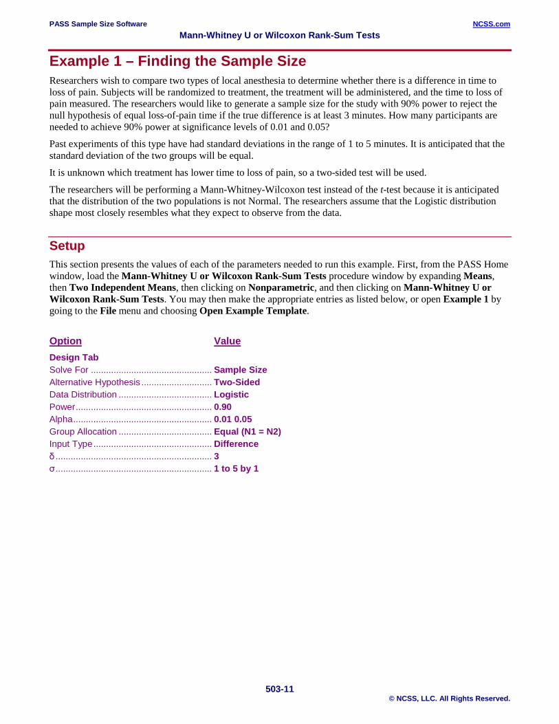
Example 1 – Finding the Sample Size Researchers wish to compare two types of local anesthesia to determine whether there is a difference in time to loss of pain. Subjects will be randomized to treatment, the treatment will be administered, and the time to loss of pain measured. The researchers would like to generate a sample size for the study with 90% power to reject the null hypothesis of equal loss-of-pain time if the true difference is at least 3 minutes. How many participants are needed to achieve 90% power at significance levels of 0.01 and 0.05?

Past experiments of this type have had standard deviations in the range of 1 to 5 minutes. It is anticipated that the standard deviation of the two groups will be equal.

It is unknown which treatment has lower time to loss of pain, so a two-sided test will be used.

The researchers will be performing a Mann-Whitney-Wilcoxon test instead of the t-test because it is anticipated that the distribution of the two populations is not Normal. The researchers assume that the Logistic distribution shape most closely resembles what they expect to observe from the data.

Setup This section presents the values of each of the parameters needed to run this example. First, from the PASS Home window, load the Mann-Whitney U or Wilcoxon Rank-Sum Tests procedure window by expanding Means, then Two Independent Means, then clicking on Nonparametric, and then clicking on Mann-Whitney U or Wilcoxon Rank-Sum Tests. You may then make the appropriate entries as listed below, or open Example 1 by going to the File menu and choosing Open Example Template.

Option Value Design Tab Solve For ................................................ Sample Size Alternative Hypothesis ............................ Two-Sided Data Distribution ..................................... Logistic Power ...................................................... 0.90 Alpha ....................................................... 0.01 0.05 Group Allocation ..................................... Equal (N1 = N2) Input Type ............................................... Difference δ .............................................................. 3 σ .............................................................. 1 to 5 by 1




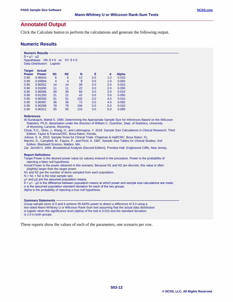
Annotated Output Click the Calculate button to perform the calculations and generate the following output.

Numeric Results

Numeric Results ──────────────────────────────────────────────────────────── δ = μ1 - μ2 Hypotheses: H0: δ ≠ 0 vs. H1: δ ≠ 0 Data Distribution: Logistic Target Actual Power Power N1 N2 N δ σ Alpha 0.90 0.95643 6 6 12 3.0 1.0 0.010 0.90 0.93894 4 4 8 3.0 1.0 0.050 0.90 0.90052 14 14 28 3.0 2.0 0.010 0.90 0.91690 11 11 22 3.0 2.0 0.050 0.90 0.90596 30 30 60 3.0 3.0 0.010 0.90 0.91250 21 21 42 3.0 3.0 0.050 0.90 0.90260 51 51 102 3.0 4.0 0.010 0.90 0.90487 36 36 72 3.0 4.0 0.050 0.90 0.90268 78 78 156 3.0 5.0 0.010 0.90 0.90312 55 55 110 3.0 5.0 0.050 References Al-Sunduqchi, Mahdi S. 1990. Determining the Appropriate Sample Size for Inferences Based on the Wilcoxon Statistics. Ph.D. dissertation under the direction of William C. Guenther, Dept. of Statistics, University of Wyoming, Laramie, Wyoming. Chow, S.C., Shao, J., Wang, H., and Lokhnygina, Y. 2018. Sample Size Calculations in Clinical Research, Third Edition. Taylor & Francis/CRC. Boca Raton, Florida. Julious, S. A. 2010. Sample Sizes for Clinical Trials. Chapman & Hall/CRC. Boca Raton, FL. Machin, D., Campbell, M., Fayers, P., and Pinol, A. 1997. Sample Size Tables for Clinical Studies, 2nd Edition. Blackwell Science. Malden, MA. Zar, Jerrold H. 1984. Biostatistical Analysis (Second Edition). Prentice-Hall. Englewood Cliffs, New Jersey. Report Definitions Target Power is the desired power value (or values) entered in the procedure. Power is the probability of rejecting a false null hypothesis. Actual Power is the power obtained in this scenario. Because N1 and N2 are discrete, this value is often (slightly) larger than the target power. N1 and N2 are the number of items sampled from each population. N = N1 + N2 is the total sample size. μ1 and μ2 are the assumed population means. δ = μ1 - μ2 is the difference between population means at which power and sample size calculations are made. σ is the assumed population standard deviation for each of the two groups. Alpha is the probability of rejecting a true null hypothesis. Summary Statements ───────────────────────────────────────────────────────── Group sample sizes of 6 and 6 achieve 95.643% power to detect a difference of 3.0 using a two-sided Mann-Whitney U or Wilcoxon Rank-Sum test assuming that the actual data distribution is logistic when the significance level (alpha) of the test is 0.010 and the standard deviation is 1.0 in both groups.

These reports show the values of each of the parameters, one scenario per row.




Plots Section

These plots show the relationship between the standard deviation and sample size for the two alpha levels.




Example 2 – Comparing the Power to the T-Test with Normal Data Suppose a new corn fertilizer is to be compared to a current fertilizer. The current fertilizer produces an average of about 74 lbs. per plot. The researchers need only show that there is difference (increase) in yield with the new fertilizer. With 90 plots available, they would like to examine the power of the test if the improvement in yield is at least 10 lbs.

Researchers plan to use a one-sided test with alpha equal to 0.05. Previous studies indicate the standard deviation for plot yield to be 25 lbs. The distribution of plot yield values is unknown, so the researchers would like to see the loss in power if the distribution turns out to be Normal and the Mann-Whitney-Wilcoxon test is used rather than the standard t-test. The power for this scenario with the standard t-test is 0.594.

Setup This section presents the values of each of the parameters needed to run this example. First, from the PASS Home window, load the Mann-Whitney U or Wilcoxon Rank-Sum Tests procedure window by expanding Means, then Two Independent Means, then clicking on Nonparametric, and then clicking on Mann-Whitney U or Wilcoxon Rank-Sum Tests. You may then make the appropriate entries as listed below, or open Example 2 by going to the File menu and choosing Open Example Template. Option Value Design Tab Solve For ................................................ Power Alternative Hypothesis ............................ One-Sided Data Distribution ..................................... Normal Alpha ....................................................... 0.05 Group Allocation ..................................... Equal (N1 = N2) Sample Size Per Group .......................... 45 Input Type ............................................... Means μ1 ............................................................ 84 μ2 ............................................................ 74 σ .............................................................. 25

Output Click the Calculate button to perform the calculations and generate the following output.

Numeric Results

Numeric Results ──────────────────────────────────────────────────────────── δ = μ1 - μ2 Hypotheses: H0: δ ≤ 0 vs. H1: δ > 0 Data Distribution: Normal Power N1 N2 N μ1 μ2 δ σ Alpha 0.56868 45 45 90 84.0 74.0 10.0 25.0 0.050

The power of the Mann-Whitney test in this scenario is 0.56868. This power is only slightly less than the power of the t-test (0.594) for the corresponding scenario.




Example 3 – Validation using Chow, Shao, Wang, and Lokhnygina (2018) Chow, Shao, Wang, and Lokhnygina (2018) presents an example on page 53 of a two-sided two-sample t-test sample size calculation for equal group sizes in which δ = 0.05, σ = 0.1, alpha = 0.05, and power = 0.80. They obtain a sample size of 64 for each group.

The Mann-Whitney U or Wilcoxon Rank-Sum test power calculations are the same as the two-sample t-test except for an adjustment factor for the assumed data distribution. If we set the data distribution to Normal, we should get a result of N1 = N2 = 64 × π/3 = 67.021, which rounds up to 68.

Setup This section presents the values of each of the parameters needed to run this example. First, from the PASS Home window, load the Mann-Whitney U or Wilcoxon Rank-Sum Tests procedure window by expanding Means, then Two Independent Means, then clicking on Nonparametric, and then clicking on Mann-Whitney U or Wilcoxon Rank-Sum Tests. You may then make the appropriate entries as listed below, or open Example 3 by going to the File menu and choosing Open Example Template.

Option Value Design Tab Solve For ................................................ Sample Size Alternative Hypothesis ............................ Two-Sided Power ...................................................... 0.80 Alpha ....................................................... 0.05 Group Allocation ..................................... Equal (N1 = N2) Input Type ............................................... Difference δ .............................................................. 0.05 σ .............................................................. 0.1

Output Click the Calculate button to perform the calculations and generate the following output.

Numeric Results

Numeric Results ──────────────────────────────────────────────────────────── δ = μ1 - μ2 Hypotheses: H0: δ ≠ 0 vs. H1: δ ≠ 0 Data Distribution: Normal Target Actual Power Power N1 N2 N δ σ Alpha 0.80 0.80146 68 68 136 0.1 0.1 0.050

The sample size of 68 in each group matches the expected result.


Mann-Whitney U or Wilcoxon Rank-Sum Tests · Wilcoxon Rank-Sum test may be made using the standard...

Documents

Transcript of Mann-Whitney U or Wilcoxon Rank-Sum Tests · Wilcoxon Rank-Sum test may be made using the standard...