Manipulator trajectory planning

Václav Hlaváč Czech Technical University in Prague Faculty of Electrical Engineering Department of Cybernetics Czech Republic http://cmp.felk.cvut.cz/~hlavac

Courtesy to several authors of presentations on the web.

2

Lecture outline

We consider a robotic manipulator (open kinematic chain) for simplicity. Generalization of methods for mobile robots comes in future lectures. Problem formulation - trajectory generation. Path vs. trajectory. Path planning vs. trajectory generation. Joint space vs. operational (Cartesian) space. Via points and point to point planning / trajectory

generation. Trajectory approximation / interpolation functions.

3

Terminology: path vs. trajectory

Both terms are often confused and used as synonyms informally. Path: an ordered locus of points in the space

(either joint or operational), which the manipulator should follow. Path is a pure geometric description of motion.

Trajectory: a path on which timing law is specified, e.g., velocities and accelerations in its each point.

4

Robot Motion Planning

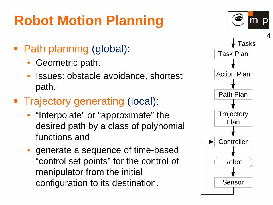
Path planning (global): • Geometric path. • Issues: obstacle avoidance, shortest

path. Trajectory generating (local):

• “Interpolate” or “approximate” the desired path by a class of polynomial functions and

• generate a sequence of time-based “control set points” for the control of manipulator from the initial configuration to its destination.

Task Plan

Action Plan

Path Plan

TrajectoryPlan

Controller

Sensor

Robot

Tasks

5

Trajectory generation, problem formulation

The aim of the trajectory generation: to generate inputs to the motion control system which ensures that the planned trajectory is executed.

The user or the upper-level planner describes the desired trajectory by some parameters, usually: • Initial and final point (point-to-point control). • Finite sequence of points along the path (motion through

sequence of points). Trajectory planning/generation can be performed

either in the joint space or operational space.

6

Minimal requirements

Capability to move robot arm and its end effector from the initial posture to the final posture.

Motion laws have to be considered in order not to: • violate saturation limits of joint drives. • excite the modeled resonant modes of the mechanical

structure. Device planning algorithm (in the sense of the

motion generation) which generates smooth trajectories. Question: Why should trajectories be smooth?

7

Joint space vs. operational space

Joint-space description: • The description of the motion to be made by the robot by

its joint values. • The motion between the two points is unpredictable.

Operational space description: • In many cases operational space = Cartesian space. • The motion between the two points is known at all times

and controllable. • It is easy to visualize the trajectory, but it is difficult to

ensure that singularity does not occur.

8

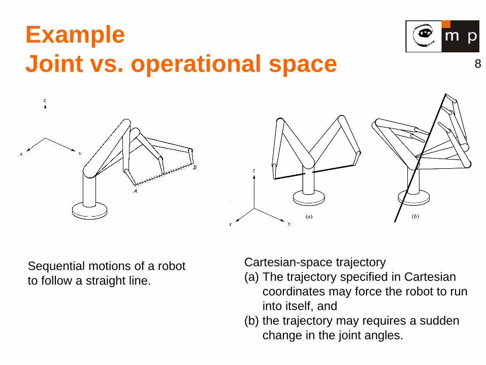
Example Joint vs. operational space

Cartesian-space trajectory (a) The trajectory specified in Cartesian

coordinates may force the robot to run into itself, and

(b) the trajectory may requires a sudden change in the joint angles.

Sequential motions of a robot to follow a straight line.

9

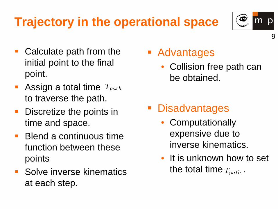
Trajectory in the operational space

Calculate path from the initial point to the final point.

Assign a total time to traverse the path.

Discretize the points in time and space.

Blend a continuous time function between these points

Solve inverse kinematics at each step.

Advantages • Collision free path can

be obtained. Disadvantages

• Computationally expensive due to inverse kinematics.

• It is unknown how to set the total time .

10

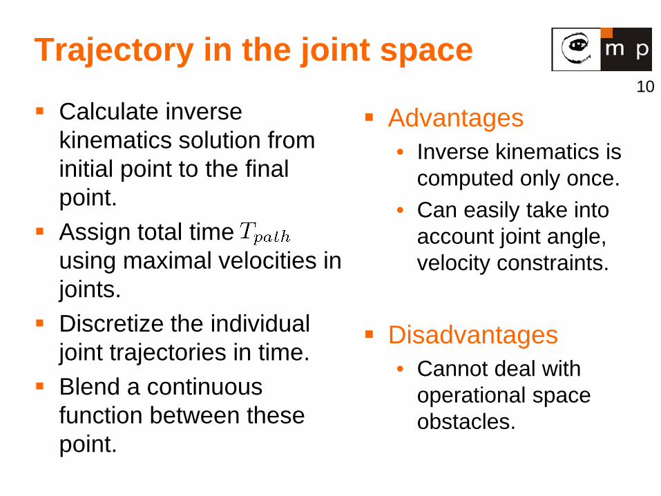
Trajectory in the joint space

Calculate inverse kinematics solution from initial point to the final point.

Assign total time using maximal velocities in joints.

Discretize the individual joint trajectories in time.

Blend a continuous function between these point.

Advantages • Inverse kinematics is

computed only once. • Can easily take into

account joint angle, velocity constraints.

Disadvantages

• Cannot deal with operational space obstacles.

11

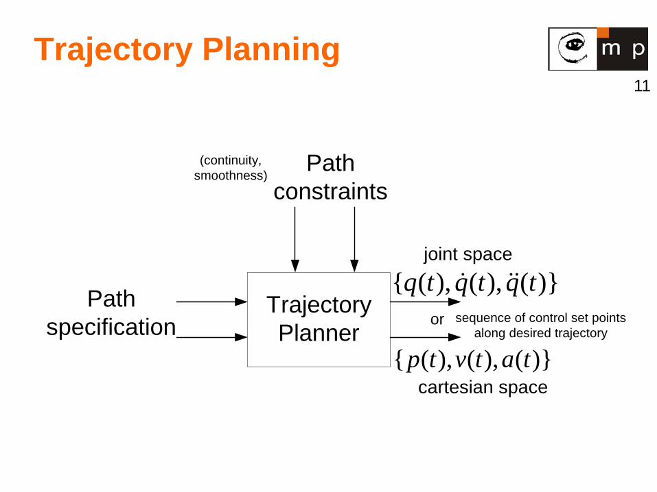
Trajectory Planning

sequence of control set pointsalong desired trajectory

(continuity,smoothness)

TrajectoryPlanner

Pathconstraints

Pathspecification

)}(),(),({ tqtqtq

)}(),(),({ tatvtp

joint space

cartesian space

or

12

The best planning approach

Combination of via points (global plan) and point to point (locally between two points). Via points provides a course approximation

of the path.

13

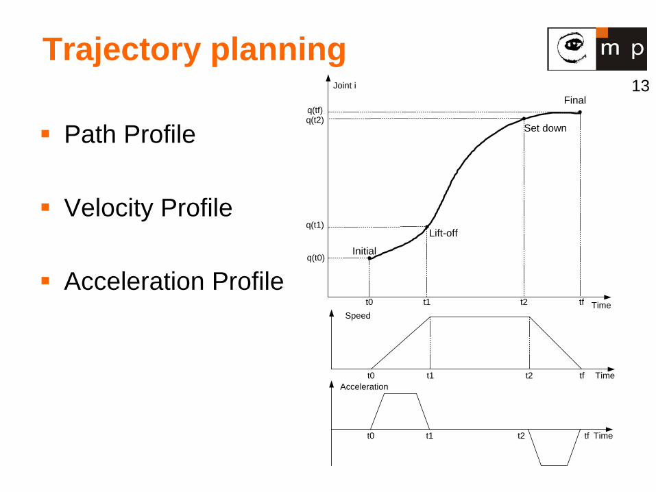
Trajectory planning

Path Profile

Velocity Profile

Acceleration Profile

t0 t1 t2 tf Time

q(t0)

q(t1)

q(t2)q(tf)

Initial

Lift-off

Set down

FinalJoint i

t0 t1 t2 tf Time

Speed

t0 t1 t2 tf Time

Acceleration

14

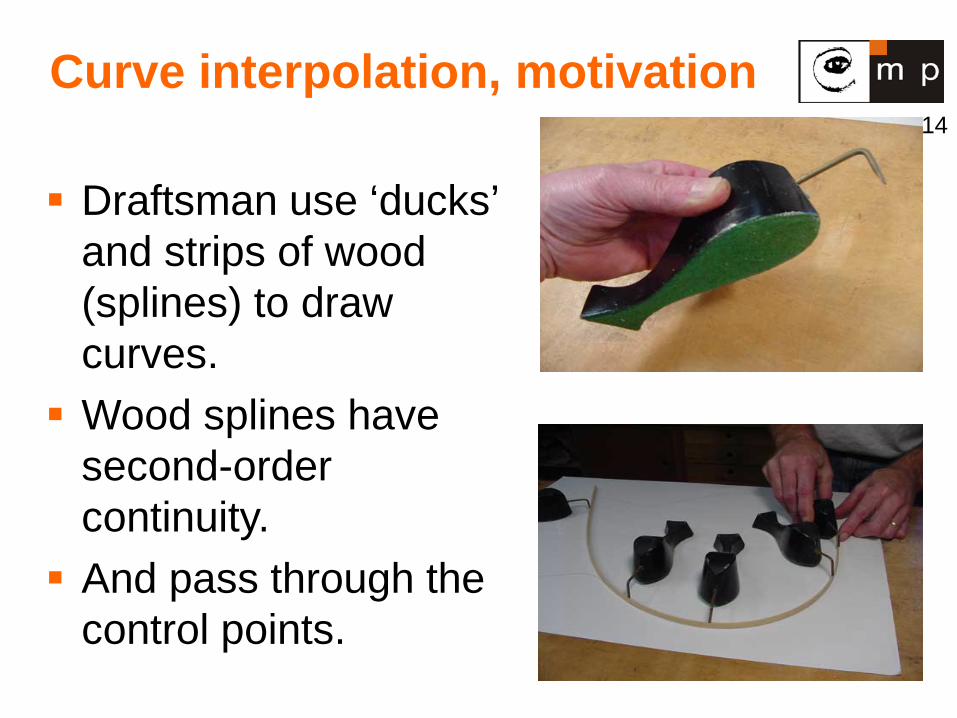
Curve interpolation, motivation

Draftsman use ‘ducks’ and strips of wood (splines) to draw curves. Wood splines have

second-order continuity. And pass through the

control points.

15

Function used for interpolation

For instance: Polynomials of different orders. Linear functions with parabolic blends. Splines.

16

Trajectory generation, basics

Different approaches will be demonstrated on a simple example

Let us consider a simple 2 degree of freedom robot.

We desire to move the robot from Point A to Point B.

Let’s assume that both joints of the robot can move at the maximum rate of 10 degree/sec.

17

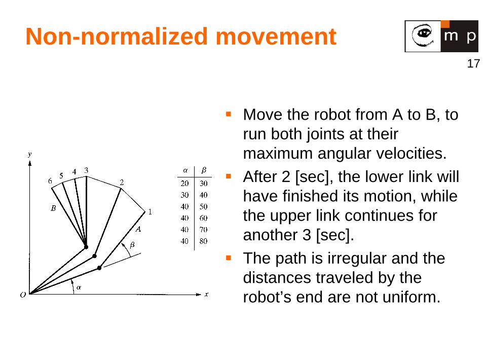
Non-normalized movement

Move the robot from A to B, to run both joints at their maximum angular velocities.

After 2 [sec], the lower link will have finished its motion, while the upper link continues for another 3 [sec].

The path is irregular and the distances traveled by the robot’s end are not uniform.

18

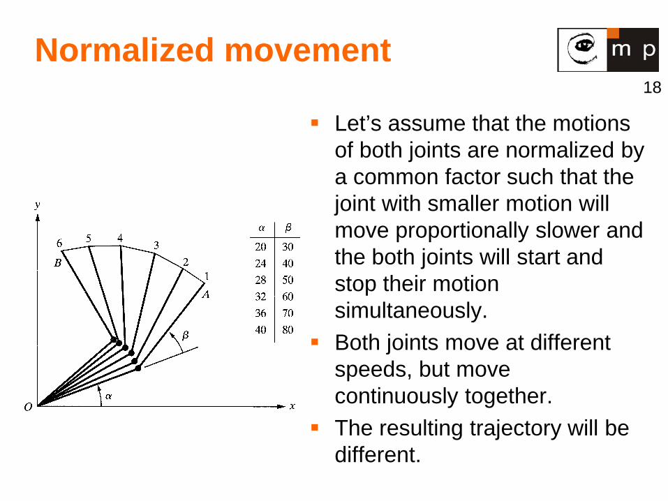
Normalized movement

Let’s assume that the motions of both joints are normalized by a common factor such that the joint with smaller motion will move proportionally slower and the both joints will start and stop their motion simultaneously.

Both joints move at different speeds, but move continuously together.

The resulting trajectory will be different.

19

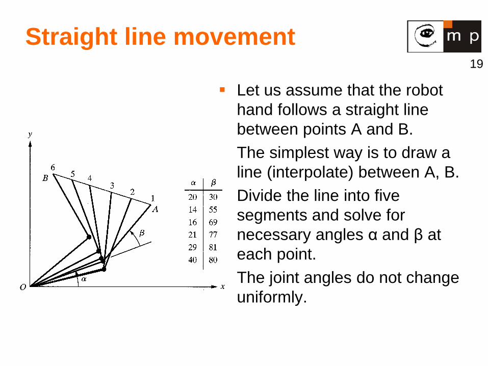
Straight line movement

Let us assume that the robot hand follows a straight line between points A and B.

The simplest way is to draw a line (interpolate) between A, B.

Divide the line into five segments and solve for necessary angles α and β at each point.

The joint angles do not change uniformly.

20

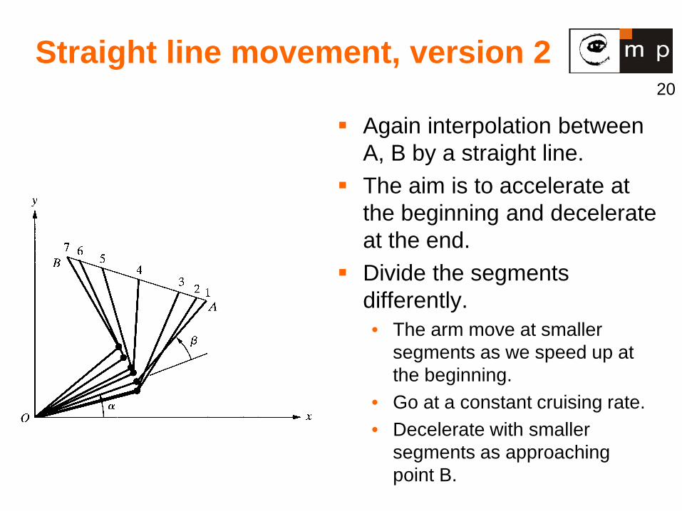
Straight line movement, version 2

Again interpolation between A, B by a straight line.

The aim is to accelerate at the beginning and decelerate at the end.

Divide the segments differently. • The arm move at smaller

segments as we speed up at the beginning.

• Go at a constant cruising rate. • Decelerate with smaller

segments as approaching point B.

21

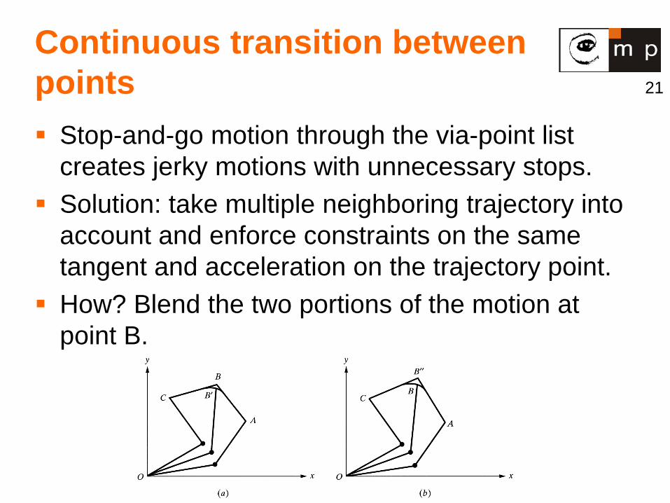
Continuous transition between points Stop-and-go motion through the via-point list

creates jerky motions with unnecessary stops. Solution: take multiple neighboring trajectory into

account and enforce constraints on the same tangent and acceleration on the trajectory point.

How? Blend the two portions of the motion at point B.

22

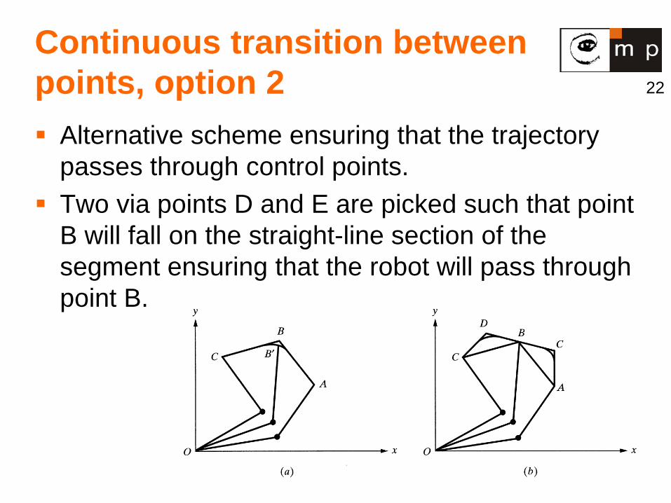
Continuous transition between points, option 2 Alternative scheme ensuring that the trajectory

passes through control points. Two via points D and E are picked such that point

B will fall on the straight-line section of the segment ensuring that the robot will pass through point B.

23

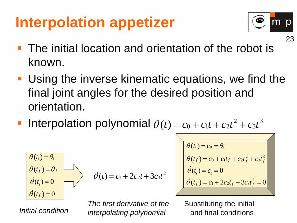
Interpolation appetizer The initial location and orientation of the robot is

known. Using the inverse kinematic equations, we find the

final joint angles for the desired position and orientation.

Interpolation polynomial

33

2210)( tctctcct +++=θ

iit θθ =)(

fft θθ =)(

( ) 0itθ =

0)( =ftθ

2321 32)( tctcct ++=θ

ii ct θθ == 0)(3

32

210)( ffff tctctcct +++=θ

1( ) 0it cθ = =

032)( 2321 =++= fff tctcctθ

Initial condition The first derivative of the interpolating polynomial

Substituting the initial and final conditions

24

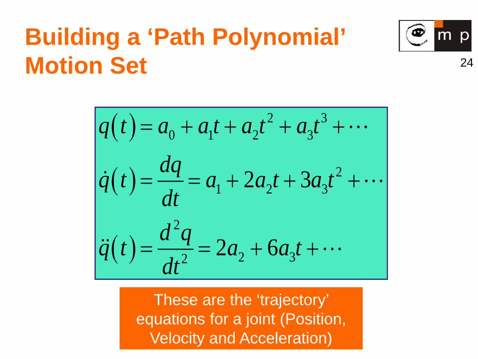
Building a ‘Path Polynomial’ Motion Set

( )

( )

( )

2 30 1 2 3

21 2 3

2

2 32

2 3

2 6

q t a a t a t a tdqq t a a t a tdtd qq t a a tdt

= + + + +

= = + + +

= = + +

These are the ‘trajectory’ equations for a joint (Position,

Velocity and Acceleration)

25

Solving the ‘Path Polynomial’ implies finding ai’s for specific paths

We would have “boundary” conditions for position and velocity at both ends of the path. We would have the desired total time of

travel. Using these conditions we can solve for

a0, a1, a2 and a3 to build a 3rd order path polynomial for the required motion.

26

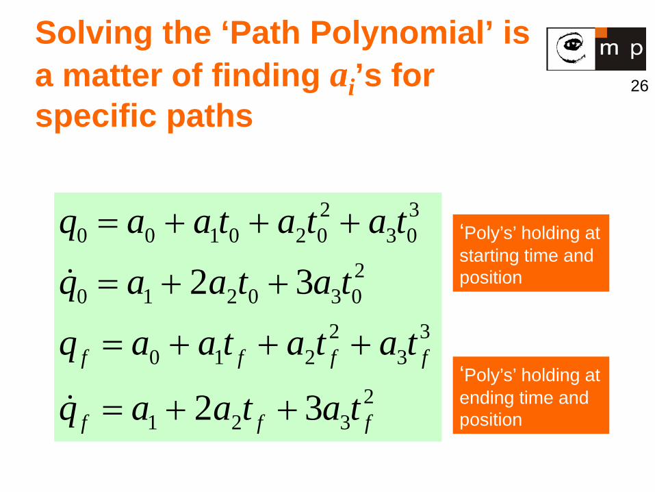
Solving the ‘Path Polynomial’ is a matter of finding ai’s for specific paths

2 30 0 1 0 2 0 3 0

20 1 2 0 3 0

2 30 1 2 3

21 2 3

2 3

2 3f f f f

f f f

q a a t a t a t

q a a t a t

q a a t a t a t

q a a t a t

= + + +

= + +

= + + +

= + +

‘Poly’s’ holding at starting time and position

‘Poly’s’ holding at ending time and position

27

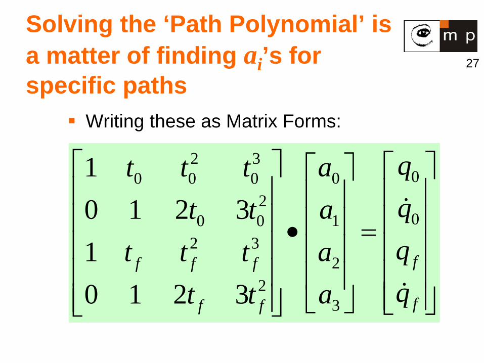
Writing these as Matrix Forms: 2 3

000 0 02

010 02 3

22

3

10 1 2 310 1 2 3

ff f f

ff f

qat t tqat tqat t tqat t

• =

Solving the ‘Path Polynomial’ is a matter of finding ai’s for specific paths

28

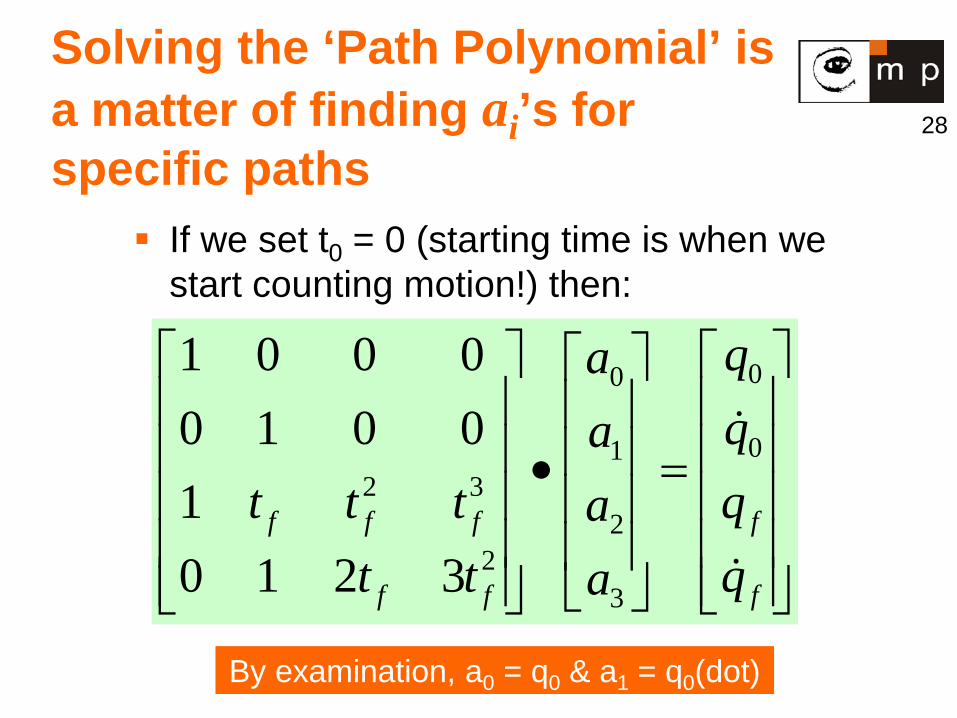
If we set t0 = 0 (starting time is when we start counting motion!) then:

00

012 3

22

3

1 0 0 00 1 0 010 1 2 3

f f f f

f f f

qaqa

t t t qat t qa

• =

By examination, a0 = q0 & a1 = q0(dot)

Solving the ‘Path Polynomial’ is a matter of finding ai’s for specific paths

29

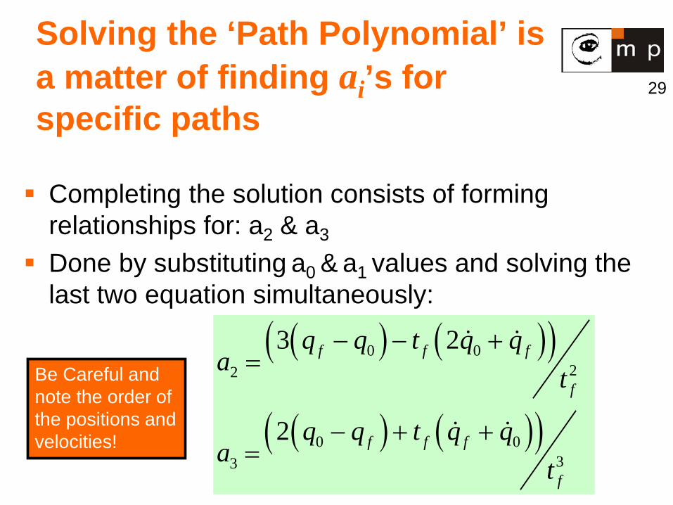
Completing the solution consists of forming relationships for: a2 & a3

Done by substituting a0 & a1 values and solving the last two equation simultaneously: ( ) ( )( )

( ) ( )( )

0 022

0 033

3 2

2

f f f

f

f f f

f

q q t q qa t

q q t q qa t

− − +=

− + +=

Be Careful and note the order of the positions and velocities!

Solving the ‘Path Polynomial’ is a matter of finding ai’s for specific paths

30

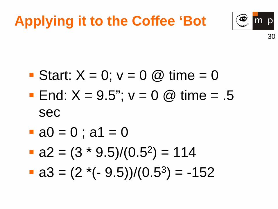
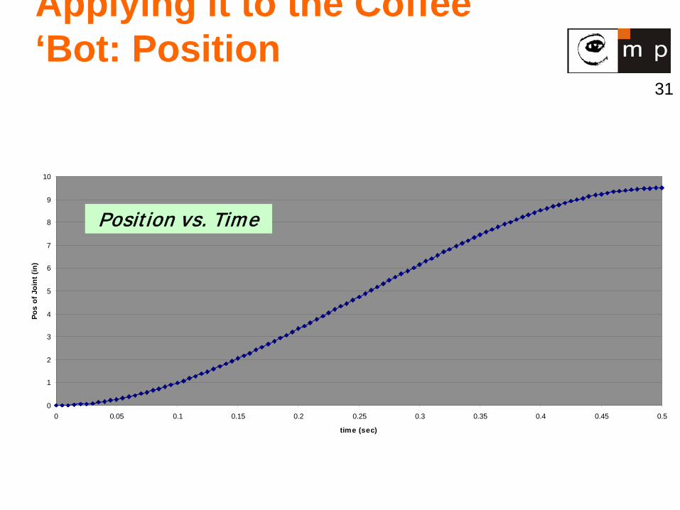
Applying it to the Coffee ‘Bot

Start: X = 0; v = 0 @ time = 0 End: X = 9.5”; v = 0 @ time = .5

sec a0 = 0 ; a1 = 0 a2 = (3 * 9.5)/(0.52) = 114 a3 = (2 *(- 9.5))/(0.53) = -152

31

Applying it to the Coffee ‘Bot: Position

0

1

2

3

4

5

6

7

8

9

10

0 0.05 0.1 0.15 0.2 0.25 0.3 0.35 0.4 0.45 0.5

time (sec)

Pos

of J

oint

(in)

Position vs. Time

32

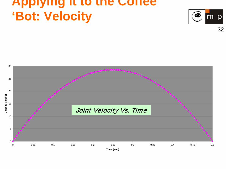
Applying it to the Coffee ‘Bot: Velocity

0

5

10

15

20

25

30

0 0.05 0.1 0.15 0.2 0.25 0.3 0.35 0.4 0.45 0.5

Time (sec)

Vel

ocity

(in/

sec)

Joint Velocity Vs. Time

33

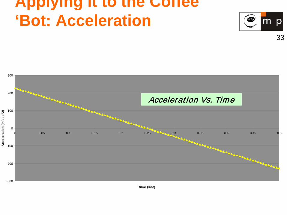
Applying it to the Coffee ‘Bot: Acceleration

-300

-200

-100

0

100

200

300

0 0.05 0.1 0.15 0.2 0.25 0.3 0.35 0.4 0.45 0.5

time (sec)

Acc

eler

atio

n (in

/sec

^2)

Acceleration Vs. Time

34

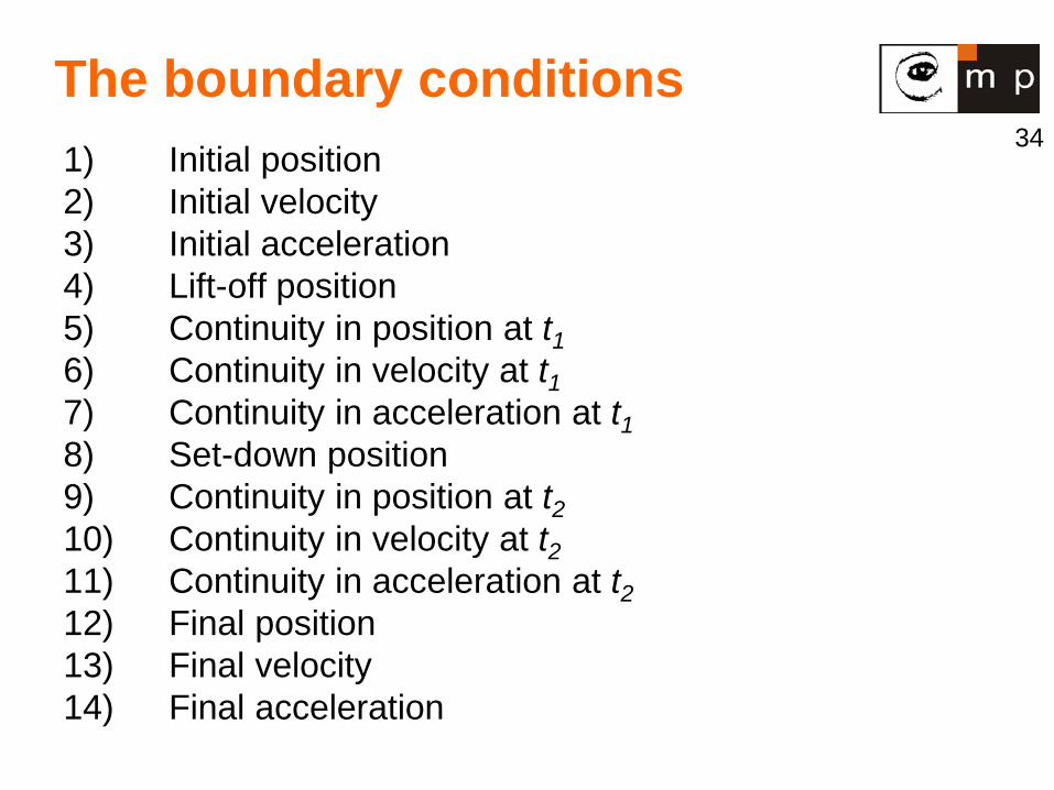
The boundary conditions 1) Initial position 2) Initial velocity 3) Initial acceleration 4) Lift-off position 5) Continuity in position at t1 6) Continuity in velocity at t1 7) Continuity in acceleration at t1 8) Set-down position 9) Continuity in position at t2 10) Continuity in velocity at t2 11) Continuity in acceleration at t2 12) Final position 13) Final velocity 14) Final acceleration

35

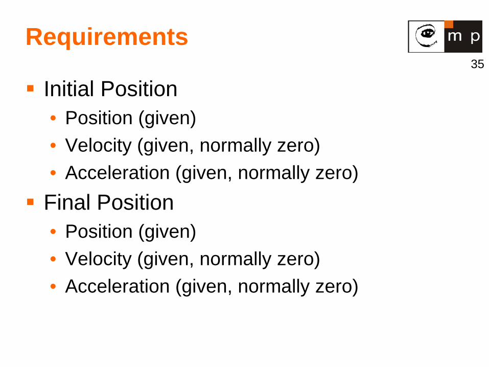
Requirements

Initial Position • Position (given) • Velocity (given, normally zero) • Acceleration (given, normally zero)

Final Position • Position (given) • Velocity (given, normally zero) • Acceleration (given, normally zero)

36

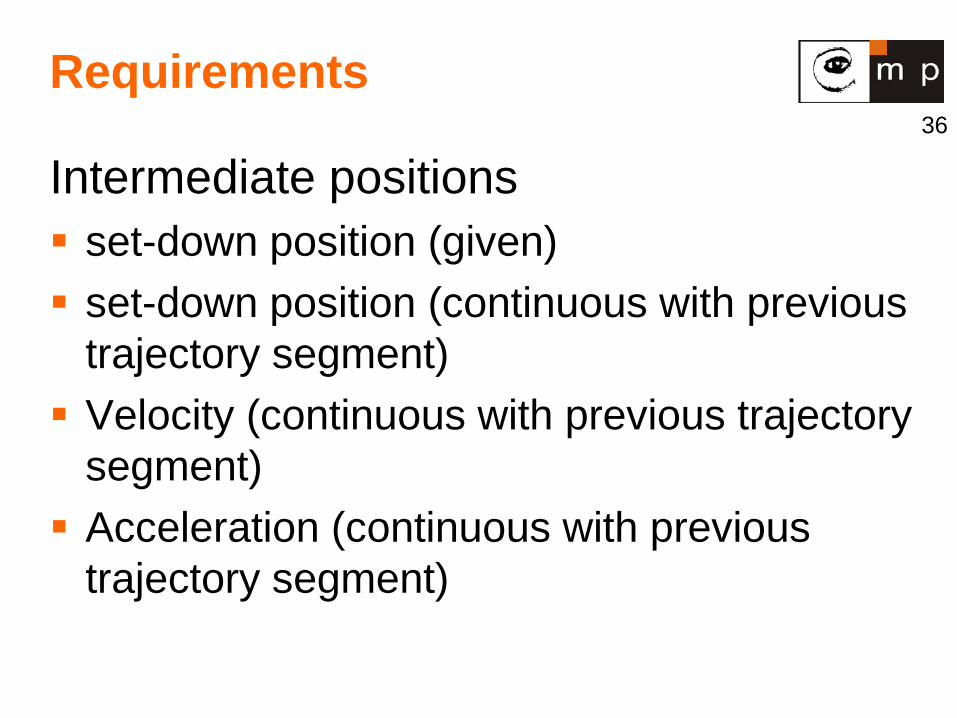
Requirements

Intermediate positions set-down position (given) set-down position (continuous with previous

trajectory segment) Velocity (continuous with previous trajectory

segment) Acceleration (continuous with previous

trajectory segment)

37

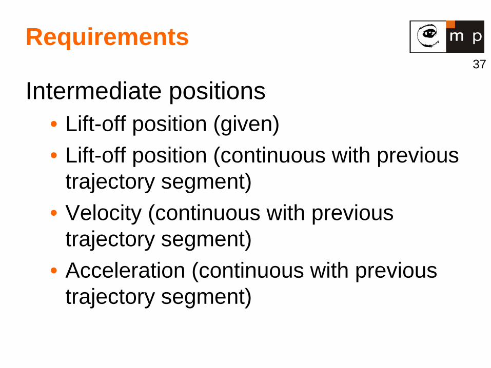
Requirements

Intermediate positions • Lift-off position (given) • Lift-off position (continuous with previous

trajectory segment) • Velocity (continuous with previous

trajectory segment) • Acceleration (continuous with previous

trajectory segment)

38

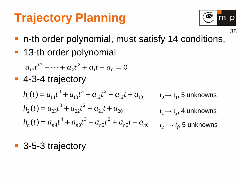
Trajectory Planning n-th order polynomial, must satisfy 14 conditions, 13-th order polynomial

4-3-4 trajectory

3-5-3 trajectory

0012

213

13 =++++ atatata

022

23

34

4

20212

223

232

10122

123

134

141

)(

)(

)(

nnnnnn atatatatathatatatath

atatatatath

++++=

+++=

++++= t0 → t1, 5 unknowns

t1 → t2, 4 unknowns

t2 → tf, 5 unknowns

39

References

B. Siciliano et al. Robotics (Modeling, planning and control), Springer, Berlin, 2009, chapter 4: Trajectory planning, pages 161-189.