Managing Production across the Supply Chain. © 2008 Pearson Prentice Hall --- Introduction to...

Managing Production across the Supply Chain

© 2008 Pearson Prentice Hall --- Introduction to Operations and Supply Chain Management, 2/e --- Bozarth and Handfield, ISBN: 0131791036

Chapter 15, Slide 2

Chapter ObjectivesBe able to: Explain the activities that make up planning and control in a

typical manufacturing environment. Explain the linkage between sales and operations planning

(S&OP) and master scheduling. Complete the calculations for the master schedule record and

interpret the results. Explain the linkage between master scheduling and material

requirements planning (MRP). Complete the calculations for the MRP record and interpret the

results. Discuss the role of production activity control and vendor order

management and how these functions differ from the higher-level planning activities.

Explain how distribution requirements planning (DRP) helps synchronize the supply chain, and complete the calculations for a simple example.


Chapter 15, Slide 3

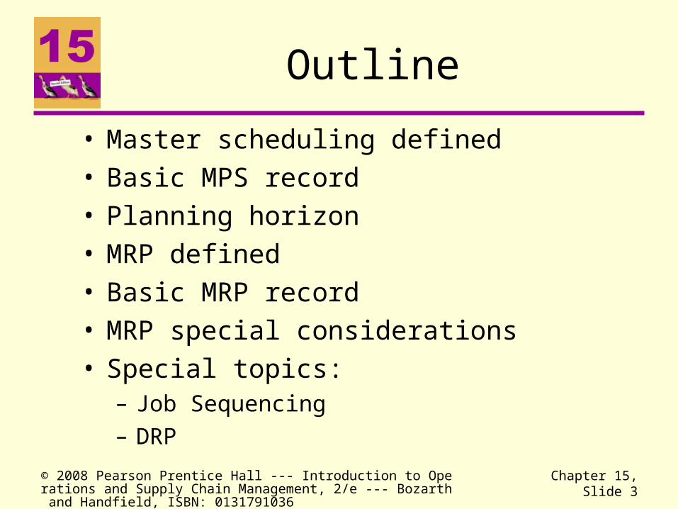
Outline

• Master scheduling defined• Basic MPS record• Planning horizon• MRP defined• Basic MRP record• MRP special considerations• Special topics:

– Job Sequencing– DRP


Chapter 15, Slide 4

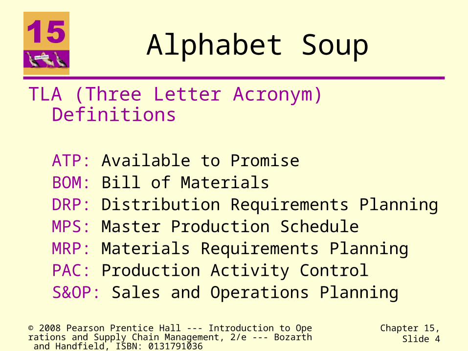
Alphabet Soup

TLA (Three Letter Acronym) Definitions

ATP: Available to PromiseBOM: Bill of MaterialsDRP: Distribution Requirements PlanningMPS: Master Production ScheduleMRP: Materials Requirements PlanningPAC: Production Activity ControlS&OP: Sales and Operations Planning


Chapter 15, Slide 5

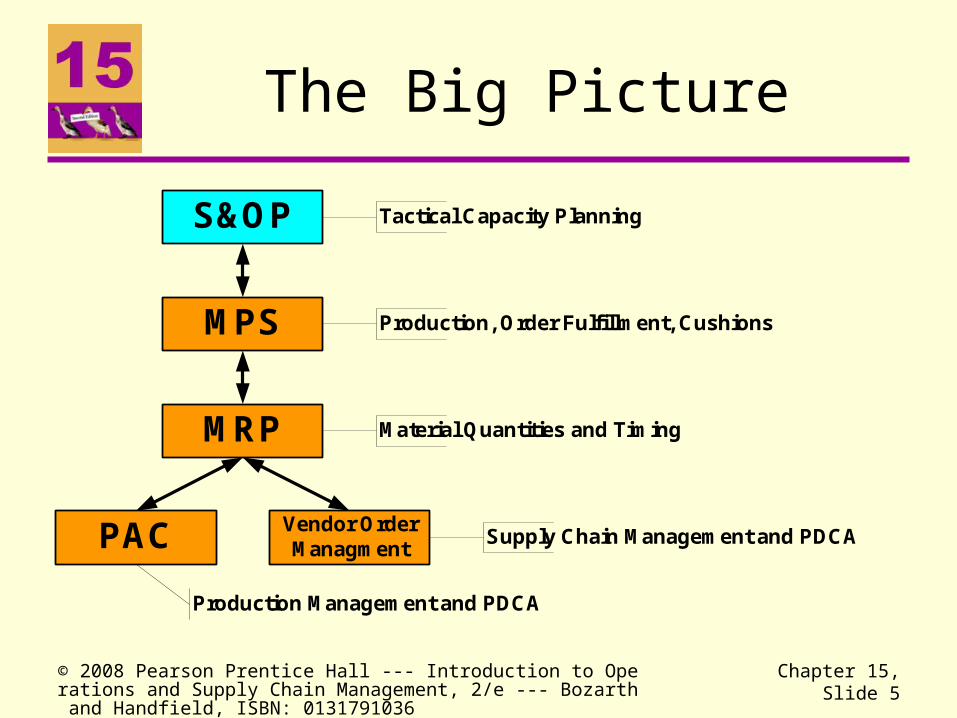
The Big Picture

S&OP

MPS

MRP

Vendor OrderManagmentPAC

Tactical Capacity Planning

Production, Order Fulfillment, Cushions

Material Quantities and Timing

Supply Chain Management and PDCA

Production Management and PDCA


Chapter 15, Slide 6

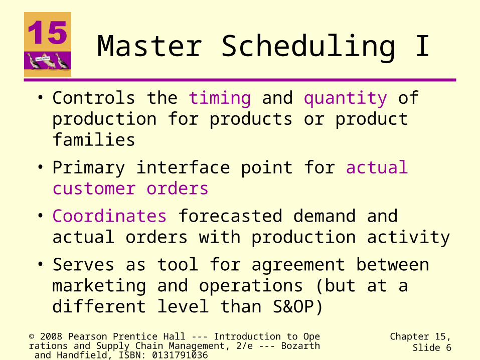
Master Scheduling I

• Controls the timing and quantity of production for products or product families

• Primary interface point for actual customer orders

• Coordinates forecasted demand and actual orders with production activity

• Serves as tool for agreement between marketing and operations (but at a different level than S&OP)


Chapter 15, Slide 7

Master Scheduling II

• Feeds data to more detailed material planning

• Indicates the quantity and timing (i.e., delivery times) for a product or group of products

• More detailed than S&OP

weekly versus monthly

specific products versus “average”


Chapter 15, Slide 8

Link between S&OP and MPS

Month: January February MarchOutput: 200 300 400

Push Mowers 25 25 25 25Self-propelled 35 40Riding 12 13

January (weeks) 1 2 3 4

S&OP

MPS


Chapter 15, Slide 9

Master Scheduling Criteria

The Master Production Schedule must:

Satisfy the needs of marketing

Be feasible for operations

Match with supply chain capability


Chapter 15, Slide 10

MPS Formulas: Definitions

• ATPt = Available to promise in period t

• EIt = Ending Inventory for period t (same as projected on-hand inventory for next period)

• Ft = Forecasted demand for period t

• MPSt = MPS quantity available in period t

• OBt = orders booked for period t



MPS Formulas:

dueisMPSpositivenextwhenperiodzwhere

OBMPSEIATP

OBFMPSEIEI

t

z

tiittt

ttttt

1

1

1 ),max(



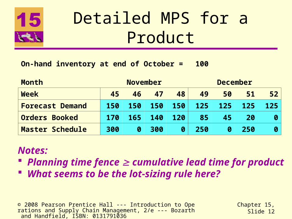
Detailed MPS for a Product

Notes: Planning time fence cumulative lead time for product What seems to be the lot-sizing rule here?

On-hand inventory at end of October = 100

Month November December

Week 45 46 47 48 49 50 51 52

Forecast Demand 150 150 150 150 125 125 125 125

Orders Booked 170 165 140 120 85 45 20 0

Master Schedule 300 0 300 0 250 0 250 0



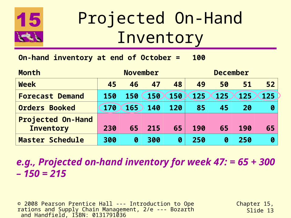
Projected On-Hand Inventory



Week 45 46 47 48 49 50 51 52

Forecast Demand 150 150 150 150 125 125 125 125

Orders Booked 170 165 140 120 85 45 20 0

Projected On-Hand Inventory 230 65 215 65 190 65 190 65

Master Schedule 300 0 300 0 250 0 250 0

e.g., Projected on-hand inventory for week 47: = 65 + 300 – 150 = 215



Available-to-Promise

ATP (Week 45) = 100 + 300 – (170 + 165) = 65ATP (Week 47) = 300 – (140+120) = 40ATP (Week 49) = 250 – (85 + 45) = 120



Week 45 46 47 48 49 50 51 52

Forecast Demand 150 150 150 150 125 125 125 125

Orders Booked 170 165 140 120 85 45 20 0


Master schedule 300 0 300 0 250 0 250 0

Available-to-Promise 65 40 120 230



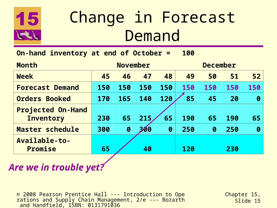
Change in Forecast Demand

Are we in trouble yet?



Week 45 46 47 48 49 50 51 52

Forecast Demand 150 150 150 150 150 150 150 150

Orders Booked 170 165 140 120 85 45 20 0


Master schedule 300 0 300 0 250 0 250 0




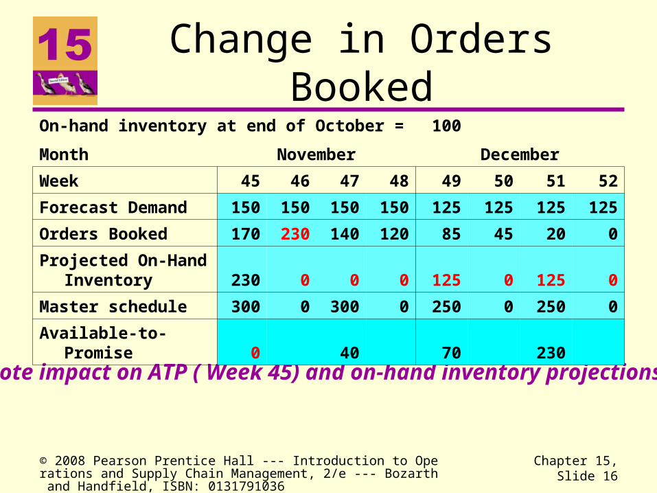
Change in Orders Booked

Note impact on ATP ( Week 45) and on-hand inventory projections



Week 45 46 47 48 49 50 51 52

Forecast Demand 150 150 150 150 125 125 125 125

Orders Booked 170 230 140 120 85 45 20 0


Master schedule 300 0 300 0 250 0 250 0




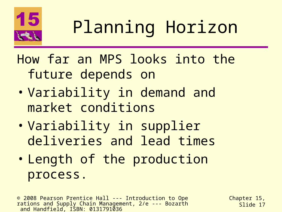
Planning Horizon

How far an MPS looks into the future depends on

• Variability in demand and market conditions

• Variability in supplier deliveries and lead times

• Length of the production process.



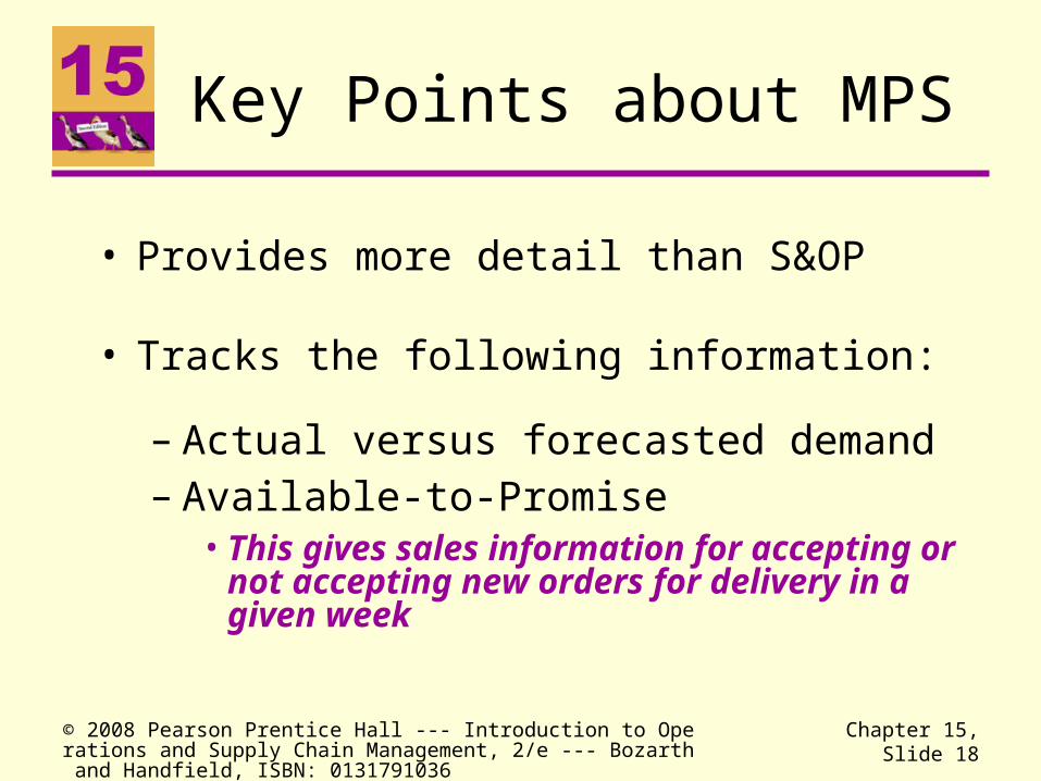
Key Points about MPS

• Provides more detail than S&OP

• Tracks the following information:

– Actual versus forecasted demand– Available-to-Promise

• This gives sales information for accepting or not accepting new orders for delivery in a given week



A Final View of Master Scheduling

S&OP

MPS

MarketingOperations & Supply Chain

Rough-Cut Capacity Plan



Material Requirements Planning

• MRP in the planning cycle

• The logic of MRP

– an extended example

• Considerations of MRP



So Far ...

We have only considered labor, overall inventory levels, and equipment:

S&OP Master scheduling Rough-Cut Capacity

Planning

But we haven’t ordered the materials!



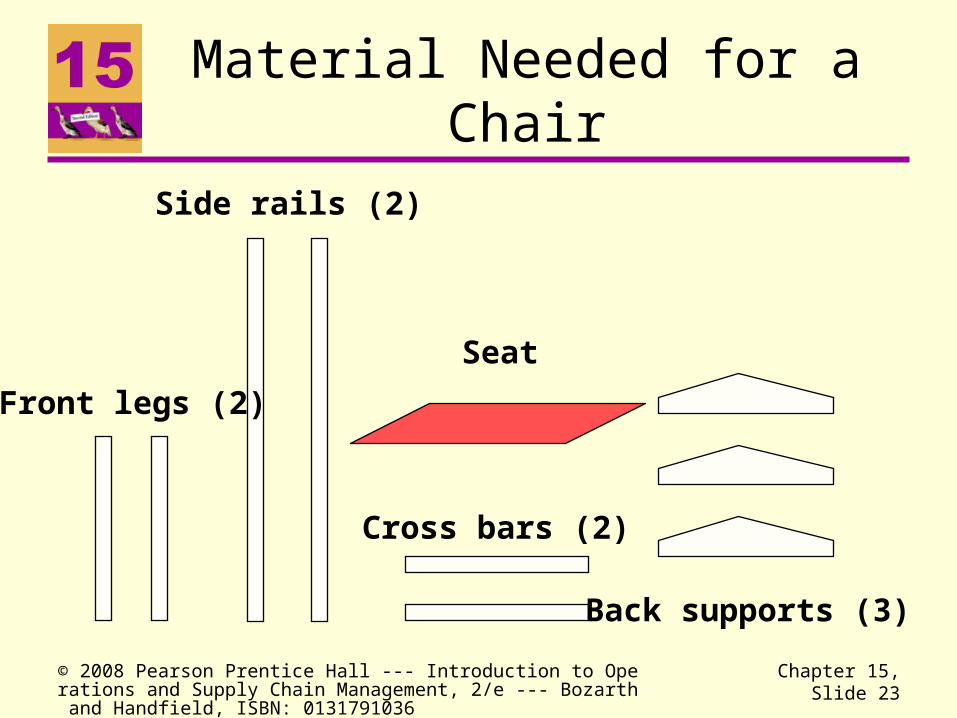
We’ve scheduled 500 chairs to be ready five weeks from now . . .

. . . Now what?



Back supports (3)

Side rails (2)

Front legs (2)

Cross bars (2)

Seat

Material Needed for a Chair



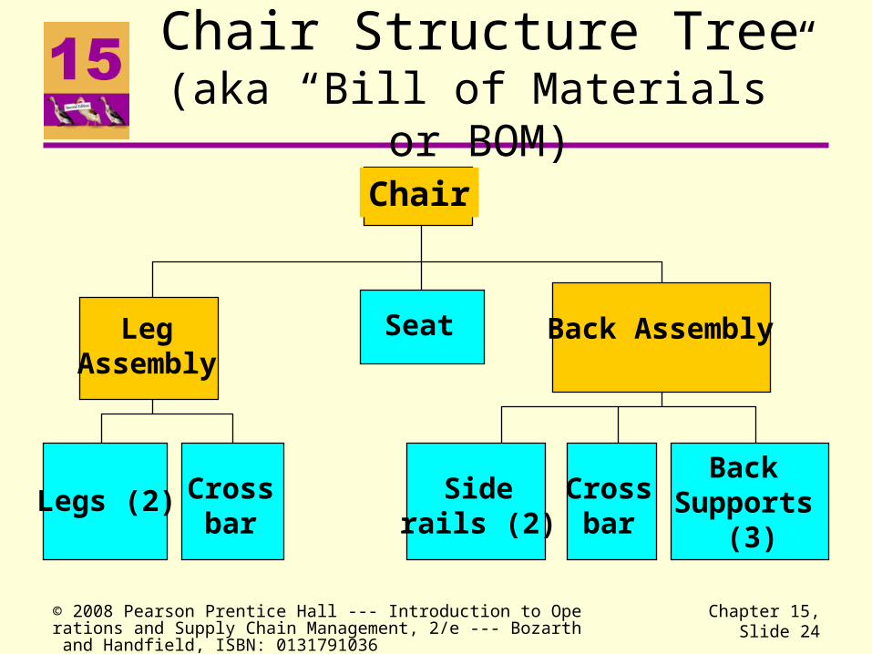
Chair Structure Tree(aka “Bill of Materials” or BOM)

Chair

LegAssembly

Seat Back Assembly

Legs (2) Crossbar

Siderails (2)

Crossbar

BackSupports

(3)



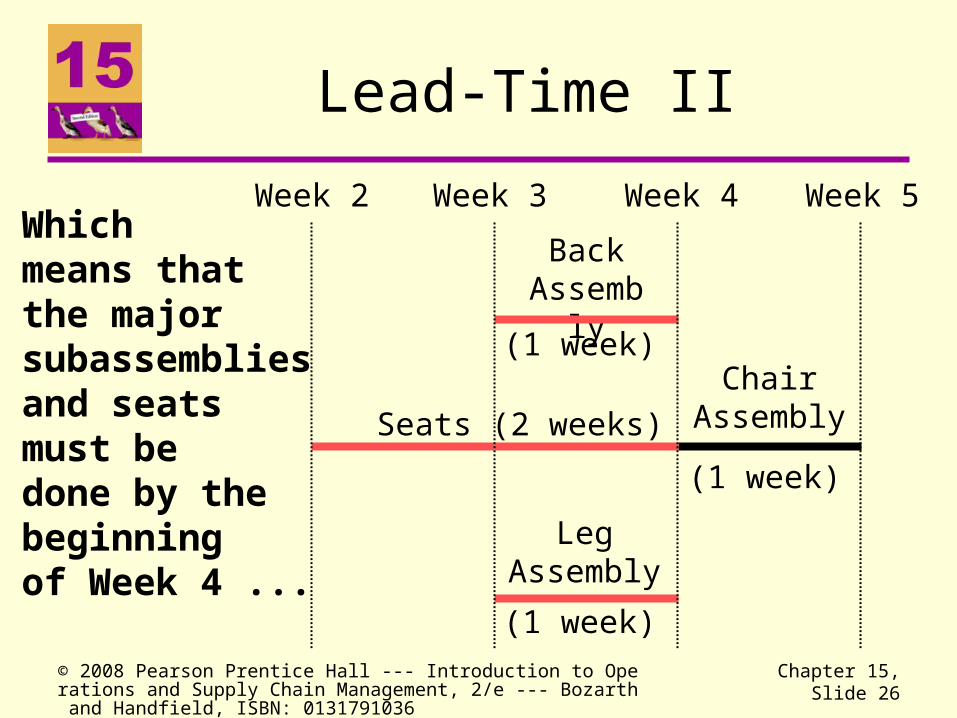
ChairAssembly

(1 week)

Week 5Week 4

If final assembly takes one week, then we must startthe assembly at the beginningof Week 4 . . .

Lead-Time I



ChairAssembly

BackAssembly

LegAssembly

(1 week)

(1 week)

(1 week)

Seats (2 weeks)

Week 5Week 4Week 3Week 2Whichmeans thatthe majorsubassembliesand seats must bedone by thebeginningof Week 4 ...

Lead-Time II



ChairAssembly

BackAssembly

LegAssembly

(1 week)

(1 week)

(1 week)

Back Support (2 weeks)

Legs (2 weeks)

Side Rails (2 weeks)

Cross Bar (2 weeks)

Cross Bar (2 weeks)

Seats (2 weeks)

Week 5Week 4Week 3Week 2Week 1

Lead-Time III



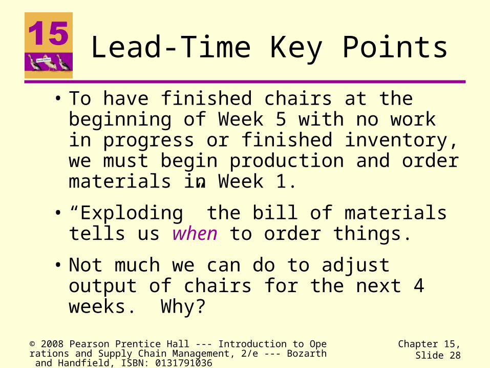
Lead-Time Key Points

• To have finished chairs at the beginning of Week 5 with no work in progress or finished inventory, we must begin production and order materials in Week 1.

• “Exploding” the bill of materials tells us when to order things.

• Not much we can do to adjust output of chairs for the next 4 weeks. Why?



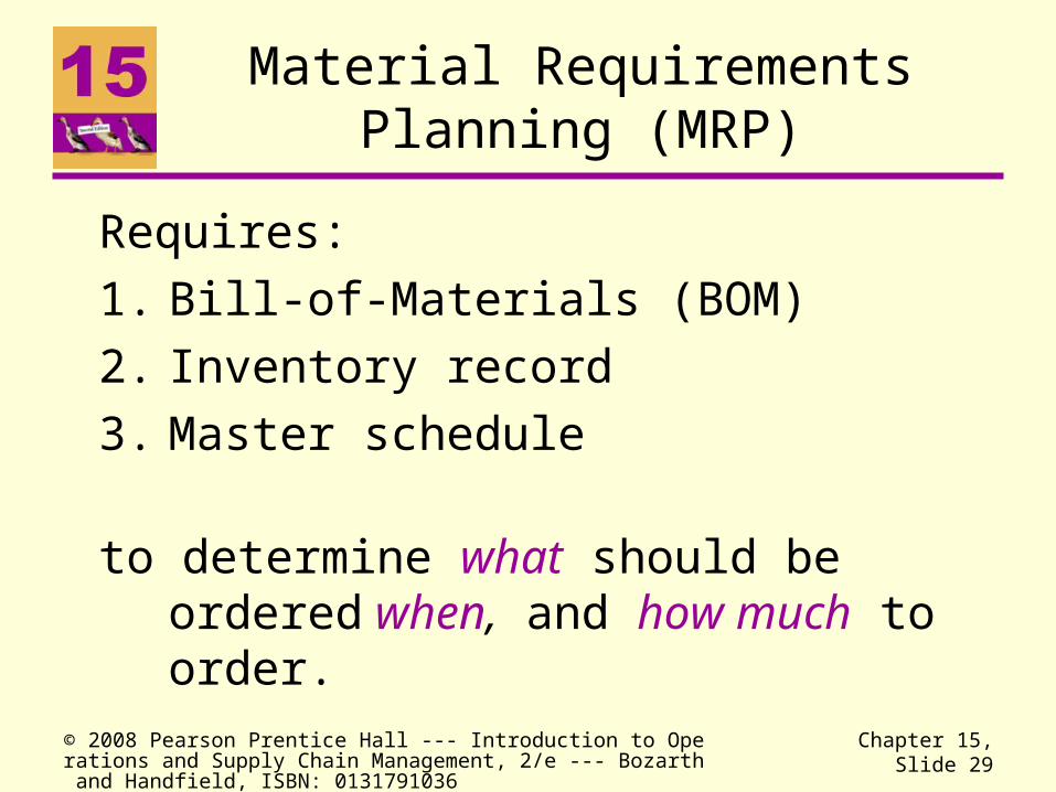
Material Requirements Planning (MRP)

Requires:

1. Bill-of-Materials (BOM)

2. Inventory record

3. Master schedule

to determine what should be ordered when, and how much to order.



End items are also known as “Level 0” items

The MRP Process Starts with the MPS

Chairs Lead Time = 1 week

1 2 3 4 5 6 7MPS Due Date 0 0 0 0 500 400 400Start Assembly 0 0 0 500 400 400 0

Week



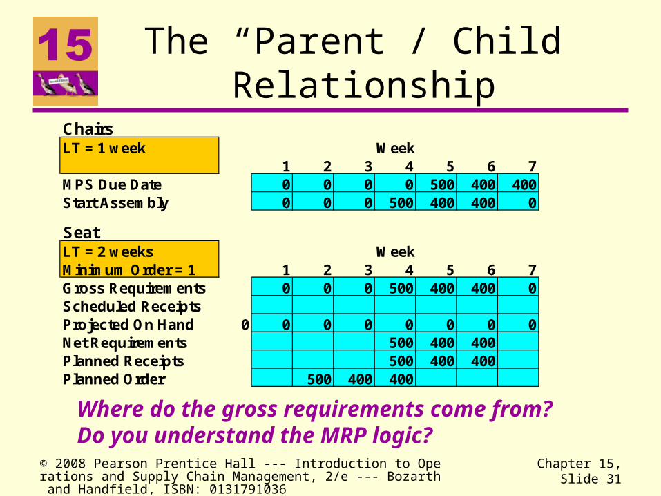
Where do the gross requirements come from?Do you understand the MRP logic?

The “Parent / Child” Relationship

ChairsLT = 1 week


SeatLT = 2 weeksMinimum Order = 1 1 2 3 4 5 6 7Gross Requirements 0 0 0 500 400 400 0Scheduled ReceiptsProjected On Hand 0 0 0 0 0 0 0 0Net Requirements 500 400 400Planned Receipts 500 400 400Planned Order 500 400 400

Week

Week



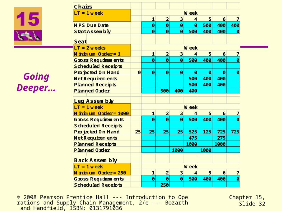
Going Deeper…

ChairsLT = 1 week


SeatLT = 2 weeksMinimum Order = 1 1 2 3 4 5 6 7Gross Requirements 0 0 0 500 400 400 0Scheduled ReceiptsProjected On Hand 0 0 0 0 0 0 0 0Net Requirements 500 400 400Planned Receipts 500 400 400Planned Order 500 400 400

Leg AssemblyLT = 1 weekMinimum Order = 1000 1 2 3 4 5 6 7Gross Requirements 0 0 0 500 400 400 0Scheduled ReceiptsProjected On Hand 25 25 25 25 525 125 725 725Net Requirements 475 275Planned Receipts 1000 1000Planned Order 1000 1000

Back AssemblyLT = 1 weekMinimum Order = 250 1 2 3 4 5 6 7Gross Requirements 0 0 0 500 400 400 0Scheduled Receipts 250

Week

Week

Week

Week



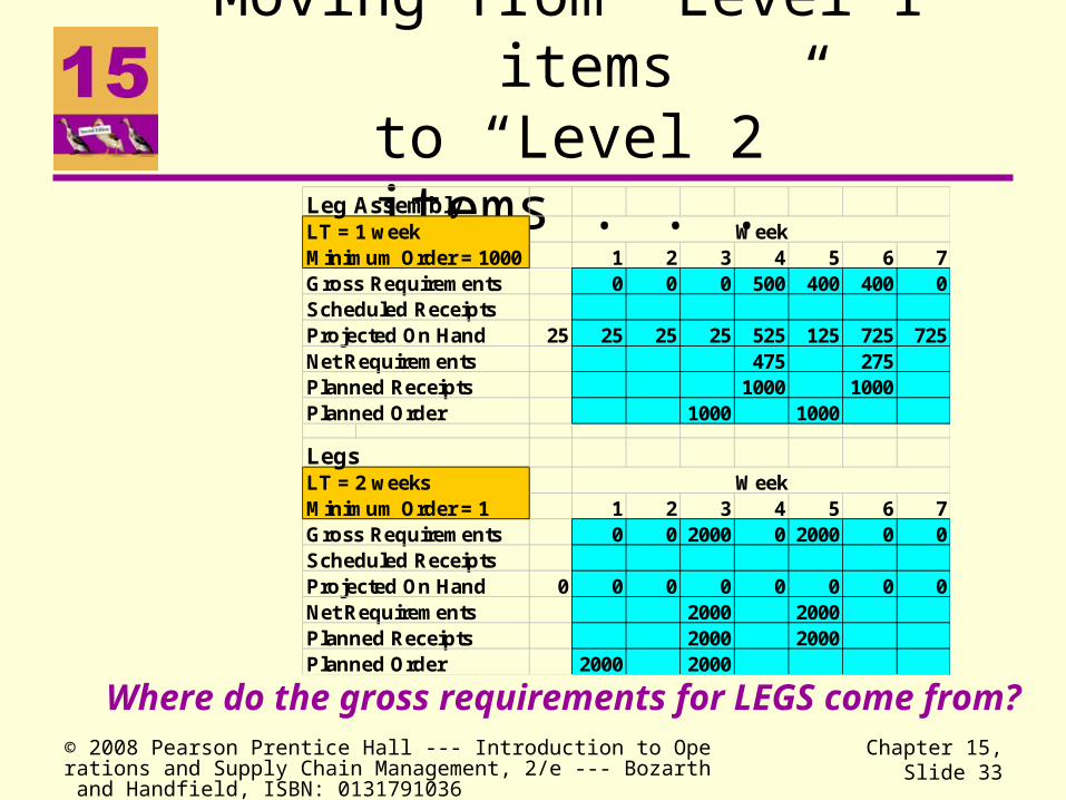
Where do the gross requirements for LEGS come from?

Moving from “Level 1” itemsto “Level 2” items . . . Leg AssemblyLT = 1 weekMinimum Order = 1000 1 2 3 4 5 6 7Gross Requirements 0 0 0 500 400 400 0Scheduled ReceiptsProjected On Hand 25 25 25 25 525 125 725 725Net Requirements 475 275Planned Receipts 1000 1000Planned Order 1000 1000

LegsLT = 2 weeksMinimum Order = 1 1 2 3 4 5 6 7Gross Requirements 0 0 2000 0 2000 0 0Scheduled ReceiptsProjected On Hand 0 0 0 0 0 0 0 0Net Requirements 2000 2000Planned Receipts 2000 2000Planned Order 2000 2000

Week

Week



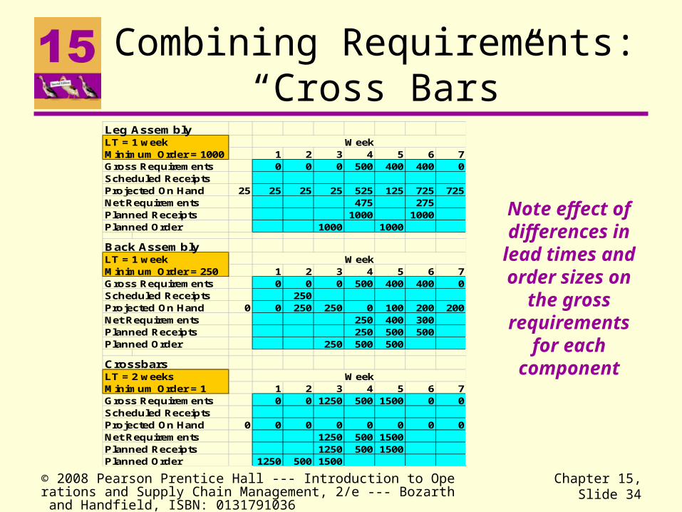
Combining Requirements: “Cross Bars”

Note effect of differences in lead times and order sizes on

the gross requirements

for each component


Back AssemblyLT = 1 weekMinimum Order = 250 1 2 3 4 5 6 7Gross Requirements 0 0 0 500 400 400 0Scheduled Receipts 250Projected On Hand 0 0 250 250 0 100 200 200Net Requirements 250 400 300Planned Receipts 250 500 500Planned Order 250 500 500

CrossbarsLT = 2 weeksMinimum Order = 1 1 2 3 4 5 6 7Gross Requirements 0 0 1250 500 1500 0 0Scheduled ReceiptsProjected On Hand 0 0 0 0 0 0 0 0Net Requirements 1250 500 1500Planned Receipts 1250 500 1500Planned Order 1250 500 1500

Week

Week

Week



Impact of Longer Lead Times

We cannot do this since the planned order would be in the past…. Thus the 250 crossbars will be delivered late one week to back assembly. What does this do to our chair schedule?


Back AssemblyLT = 2 weeksMinimum Order = 250 1 2 3 4 5 6 7Gross Requirements 0 0 0 500 400 400 0Scheduled Receipts 250Projected On Hand 0 0 250 250 0 100 200 200Net Requirements 250 400 300Planned Receipts 250 500 500Planned Order 250 500 500

CrossbarsLT = 2 weeksMinimum Order = 1 1 2 3 4 5 6 7Gross Requirements 0 250 1500 500 1000 0 0Scheduled ReceiptsProjected On Hand 0 0 0 0 0 0 0 0Net Requirements 250 1500 500 1500Planned Receipts 250 1500 500 1500Planned Order 250 1500 500 1000

Week

Week

Week



Do You Understand ...

• Why it is important to have an accurate BOM and accurate inventory information?

• Why we need to “freeze” production schedules?

• Where gross requirements come from?

• The difference between planned and scheduled receipts?



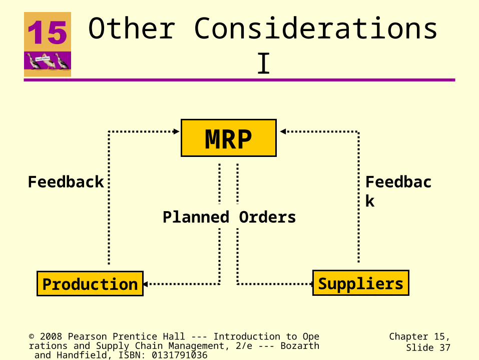
Other Considerations I

Planned Orders

Feedback Feedback

Production Suppliers

MRP



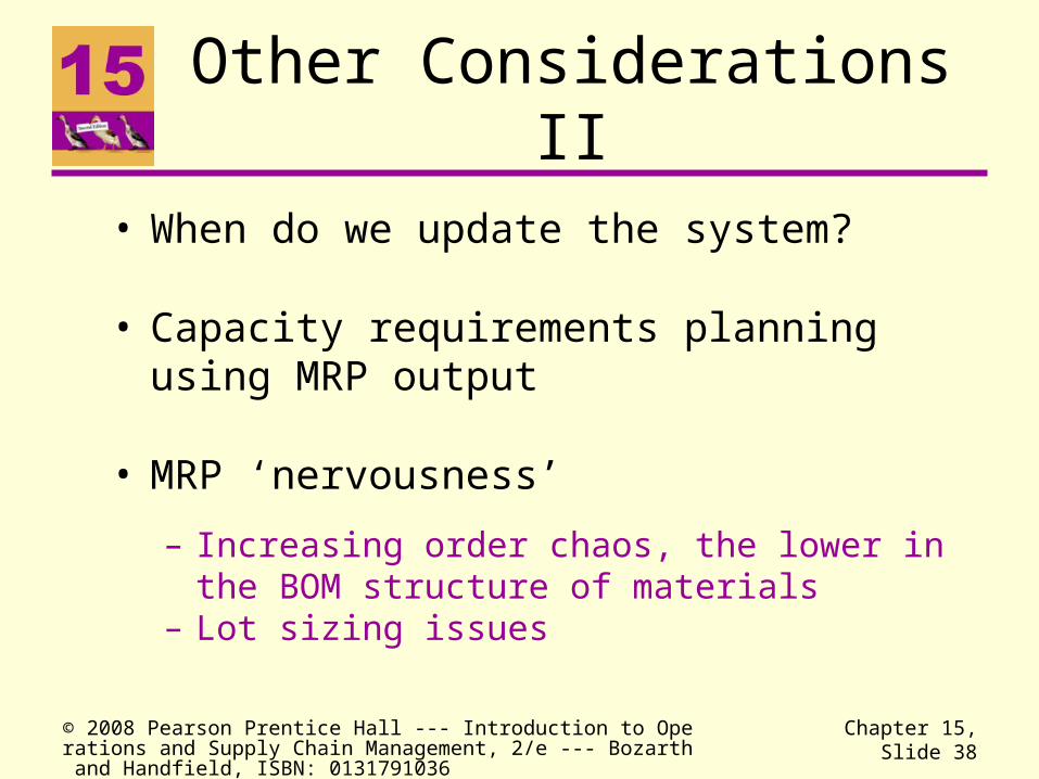
Other Considerations II

• When do we update the system?

• Capacity requirements planning using MRP output

• MRP ‘nervousness’

– Increasing order chaos, the lower in the BOM structure of materials

– Lot sizing issues



Recall ...

Look at the “lumpiness” of demand for legs


LegsLT = 2 weeksMinimum Order = 1 1 2 3 4 5 6 7Gross Requirements 0 0 2000 0 2000 0 0Scheduled ReceiptsProjected On Hand 0 0 0 0 0 0 0 0Net Requirements 2000 2000Planned Receipts 2000 2000Planned Order 2000 2000

Week

Week



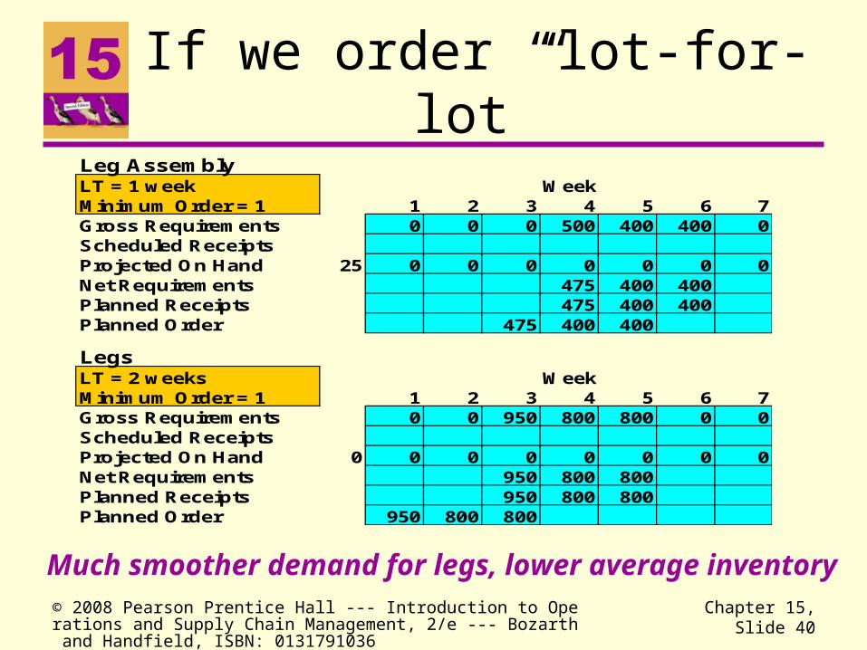
If we order “lot-for-lot”

Much smoother demand for legs, lower average inventory

Leg AssemblyLT = 1 weekMinimum Order = 1 1 2 3 4 5 6 7Gross Requirements 0 0 0 500 400 400 0Scheduled ReceiptsProjected On Hand 25 0 0 0 0 0 0 0Net Requirements 475 400 400Planned Receipts 475 400 400Planned Order 475 400 400

LegsLT = 2 weeksMinimum Order = 1 1 2 3 4 5 6 7Gross Requirements 0 0 950 800 800 0 0Scheduled ReceiptsProjected On Hand 0 0 0 0 0 0 0 0Net Requirements 950 800 800Planned Receipts 950 800 800Planned Order 950 800 800

Week

Week



Job Sequencing

• Rules:FCFS — first come, first servedEDD — earliest due dateCritical ratio — work time remaining divided

by days left before due date

• Performance measure:Average lateness — sum of days late for each

job divided by total number of jobs



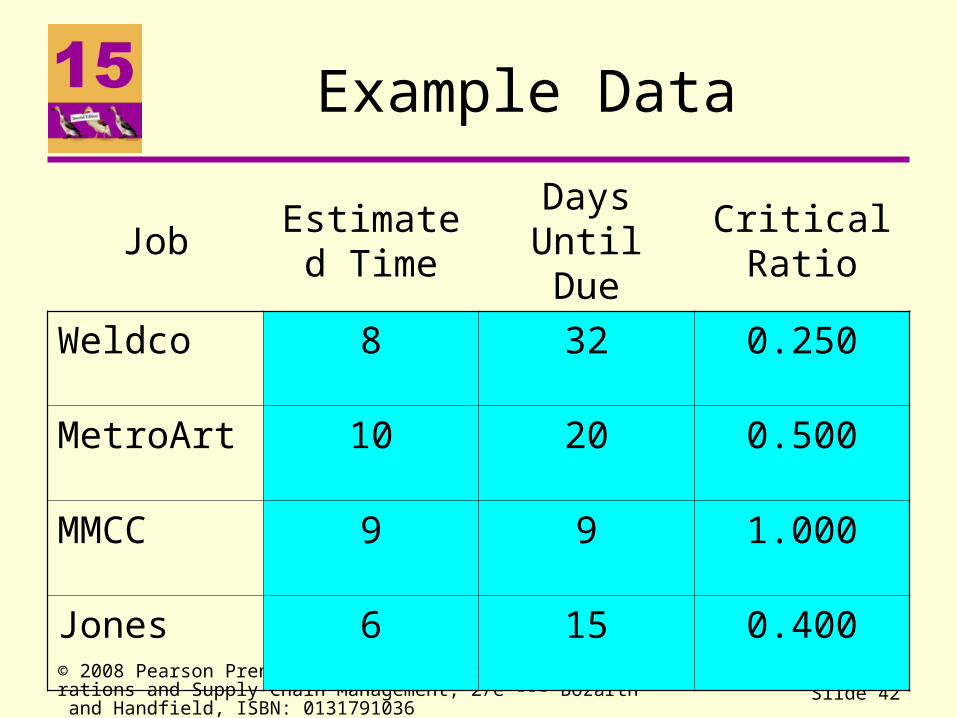
Example Data

JobEstimated

TimeDays Until

DueCritical Ratio

Weldco 8 32 0.250

MetroArt 10 20 0.500

MMCC 9 9 1.000

Jones 6 15 0.400



Example FCFS

JobEstimated

Time

Days Until Due

Start EndDays Late

Weldco 8 32 0 8 0

MetroArt 10 20 8 18 0

MMCC 9 9 18 27 18

Jones 6 15 27 33 18

Average lateness = 36/4 = 9 days



Example EDD

JobEstimated

Time

Days Until Due

Start EndDays Late

MMCC 9 9 0 9 0

Jones 6 15 9 15 0

MetroArt 10 20 15 25 5

Weldco 8 32 25 33 1

Average lateness = 6/4 = 1.5 days



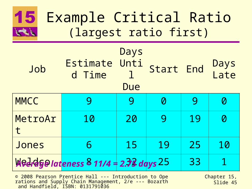
Example Critical Ratio(largest ratio first)

JobEstimated

Time

Days Until Due

Start EndDays Late

MMCC 9 9 0 9 0

MetroArt 10 20 9 19 0

Jones 6 15 19 25 10

Weldco 8 32 25 33 1

Average lateness = 11/4 = 2.75 days



Interpretation

• Here the EDD rule gives better average lateness. Compare with FCFS results.

• Note that the critical ratio does not do as well as EDD compared to the text example for Carlos Restoration. Why?



Distribution Requirements Planning (DRP)

• Anticipates downstream demand– Uses this information, not predetermined

reorder points or periodic reviews, to determine when to order

• Computer-based software systems needed to deal with the added complexity



Suppose we forecast demand for Wholesaler A for the next 8 days (the best time horizon to use will depend on many factors)

Based on this, we anticipate that Wholesaler A will order on Day 3

DRP Example I

Wholesaler A

ROP = 50, Q = 200 Day 1 Day 2 Day 3 Day 4 Day 5 Day 6 Day 7 Day 8Forecast Demand 20 20 20 20 20 20 20 20Ending Inventory 85 65 45 225 205 185 165 145 125Expected Order 200



We extend the analysis to include Wholesaler B Combined, we expect to see orders on Days 3 and 4

Wholesaler A


Wholesaler B


Total Orders 200 200

DRP Example II



The distributor then uses this information to plan its own orders. In this case, suppose it takes two days for the supplier to replenish; based on the information, the distributor would order on Day 1

Wholesaler A


Wholesaler B


Distributor

Q = 400 Day 1 Day 2 Day 3 Day 4 Day 5 Day 6 Day 7 Day 8Total Expected Orders 200 200Ending Inventory 50 50 50 250 50 50 50 50 50Planned Receipts 400Planned Orders 400

DRP Example III



DRP Benefits

Helps improve customer service Provides a better and faster understanding of

the impact of shortages and/or promotions

Helps reduce costs InventoryFreightProduction

Provides integration between the stages in the supply chain



DRP Constraints

• Accurate forecasts and inventory levels– Necessary to anticipate correctly when orders will be

placed• Consistent and reliable lead times

– To ensure that orders can be placed and arrive by the time they are needed

• “Nervousness”– Even light changes in demand for downstream partners

can have a significant impact on order volumes, especially when order sizes are relatively high

Case Study in Managing Production

The Realco Breadmaster

Managing Production across the Supply Chain. © 2008 Pearson Prentice Hall --- Introduction to...

Documents

Transcript of Managing Production across the Supply Chain. © 2008 Pearson Prentice Hall --- Introduction to...