Managing a Liquidity Trap:Monetary and Fiscal Policy∗

Iván Werning, MIT

August 2011

Abstract

I study monetary and fiscal policy in liquidity trap scenarios, where the zero bound

on the nominal interest rate is binding. I work with a continuous-time version of the

standard New Keynesian model. Without commitment the economy suffers from de-

flation and depressed output. I show that, surprisingly, both are exacerbated with

greater price flexibility. I examine monetary and fiscal policies that maximize utility

for the agent in the model and refer to these as optimal throughout the paper. I find

that the optimal interest rate is set to zero past the liquidity trap and jumps discretely

up upon exit. Inflation may be positive throughout, so the absence of deflation is not

evidence against a liquidity trap. Output, on the other hand, always starts below its

efficient level and rises above it. I then study fiscal policy and show that, regardless

of parameters that govern the value of “fiscal multipliers” during normal or liquid-

ity trap times, at the start of a liquidity trap optimal spending is above its natural

level. However, it declines over time and goes below its natural level. I propose a de-

composition of spending according to “opportunistic” and “stimulus” motives. The

former is defined as the level of government purchases that is optimal from a static,

cost-benefit standpoint, taking into account that, due to slack resources, shadow costs

may be lower during a slump; the latter measures deviations from the former. I show

that stimulus spending may be zero throughout, or switch signs, depending on pa-

rameters. Finally, I consider the hybrid where monetary policy is discretionary, but

fiscal policy has commitment. In this case, stimulus spending is typically positive and

increasing throughout the trap.

∗For useful discussions I thank Manuel Amador, George-Marios Angeletos, Emmanuel Farhi, Jordi Galíand Ricardo Reis, as well as seminar participants. All remaining errors are mine.

1

1 Introduction

The 2007-8 crisis in the U.S. lead to a steep recession, followed by aggressive policy re-sponses. Monetary policy went full tilt, cutting interest rates rapidly to zero, where theyhave remained since the end of 2008. With conventional monetary policy seemingly ex-hausted, fiscal stimulus worth $787 billion was enacted by early 2009 as part of the Amer-ican Recovery and Reinvestment Act. Unconventional monetary policies were also pur-sued, starting with “quantitative easing”, purchases of long-term bonds and other assets.In August 2011, the Federal Reserve’s FOMC statement signaled the intent to keep inter-est rates at zero until at least mid 2013. Similar policies have been followed, at least duringthe peak of the crisis, by many advanced economies. Fortunately, the kind of crises thatresult in such extreme policy measures have been relatively few and far between. Perhapsas a consequence, the debate over whether such policies are appropriate remains largelyunsettled. The purpose of this paper is to make progress on these issues.

To this end, I reexamine monetary and fiscal policy in a liquidity trap, where the zerobound on nominal interest rate binds. I work with a standard New Keynesian model thatbuilds on Eggertsson and Woodford (2003).1 In these models a liquidity trap is defined asa situation where negative real interest rates are needed to obtain the first-best allocation.I adopt a deterministic continuous time formulation that turns out to have several advan-tages. It is well suited to focus on the dynamic questions of policy, such as the optimal exitstrategy, whether spending should be front- or back-loaded, etc. It also allows for a simplegraphical analysis and delivers several new results. The alternative most employed in theliterature is a discrete-time Poisson model, where the economy starts in a trap and exitsfrom it with a constant exogenous probability each period. This specification is especiallyconvenient to study the effects of suboptimal and simple Markov policies—because theequilibrium calculations then reduce to finding a few numbers—but does not afford anycomparable advantages for the optimal policy problem.

I examine policies that maximize welfare for the agent in the model and refer to themthroughout as optimal. I consider the policy problem under commitment, under discre-tion and for some intermediate cases. I am interested in monetary policy, fiscal policy, aswell as their interplay. What does optimal monetary policy look like? How does the com-mitment solution compare to the discretionary one? How does it depend on the degree ofprice stickiness? How can fiscal policy complement optimal monetary policy? Can fiscal

1Eggertsson (2001, 2006) study government spending during a liquidity trap a New Keynesian model,with the main focus is on the case without commitment and implicit commitment to inflate afforded byrising debt. Christiano et al. (2011), Woodford (2011) and Eggertsson (2011) consider the effects of spendingon output, computing “fiscal multipliers”, but do not focus on optimal policy.

2

policy mitigate the problem created by discretionary monetary policy? To what extent isspending governed by a concern to influence the private economy as captured by "fiscalmultipliers", or by simple cost-benefit public finance considerations?

I first study monetary policy in the absence of fiscal policy. When monetary policylacks commitment, deflation and depression ensue. Both are commonly associated withliquidity traps. Less familiar is that both outcomes are exacerbated by price flexibility.Thus, one does not need to argue for a large degree of price stickiness to worry about theproblems created by a liquidity trap. In fact, quite the contrary. I show that the depressionbecomes unbounded as we converge to fully flexible prices. The intuition for this resultis that the main problem in a liquidity trap is an elevated real interest rate. This leadsto depressed output, which creates deflationary pressures. Price flexibility acceleratesdeflation, raising the real interest rate further and only making matters worse.

As first argued by Krugman (1998), optimal monetary policy can improve on this direoutcome by committing to future policy in a way that affects current expectations favor-ably. In particular, I show that, it is optimal to promote future inflation and stimulate aboom in output. I establish that optimal inflation may be positive throughout the episode,so that deflation is completely avoided. Thus, the absence of deflation, far from being atodds with a liquidity trap, actually may be evidence of an optimal response to such a situ-ation. I show that output starts below its efficient level, but rises above it towards the endof the trap. Indeed, the boom in output is larger than that stimulated by the inflationarypromise.

There are a number of ways monetary policy can promote inflation and stimulateoutput. Monetary easing does not necessarily imply a low equilibrium interest rate path.Indeed, as in most monetary models, the nominal interest rate path does not uniquelydetermine an equilibrium. Indeed, an interest rate of zero during the trap that becomespositive immediately after the trap is consistent with positive inflation and output afterthe trap.2 I show, however, that the optimal policy with commitment involves keepingthe interest rate down at zero longer. The continuous time formulation helps here becauseit avoids time aggregation issues that may otherwise obscure the result.

Some of my results echo findings from prior work based on simulations for a Poissonspecification of the natural rate of interest. Christiano et al. (2011) reports that, when thecentral bank follows a Taylor rule, price stickiness increases the decline in output during

2For example, a zero interest during the trap and an interest equal to the natural rate outside the trap.This is the same path for the interest rate that results with discretionary monetary policy. However, in thatcase, the outcome for inflation and output is pinned down by the requirement that they reach zero uponexiting the trap. With commitment, the same path for interest rates is consistent with higher inflation andoutput upon exit.

3

a liquidity trap. Eggertsson and Woodford (2003), Jung et al. (2005) and Adam and Billi(2006) find that the optimal interest rate path may keep it at zero after the natural rateof interest becomes positive. To the best of my knowledge this paper provides the firstformal results explaining these findings for inflation, output and interest rates.

An implication of my result is that the interest rate should jump discretely upon exit-ing the zero bound—a property that can only be appreciated in continuous time. Thus,even when fundamentals vary continuously, optimal policy calls for a discontinuous in-terest rate path.

Turning to fiscal policy, I show that, there is a role for government spending dur-ing a liquidity trap. Spending should be front-loaded. At the start of the liquidity trap,government spending should be higher than its natural level. However, during the trapspending should fall and reach a level below its natural level. Intuitively, optimal govern-ment spending is countercyclical, it leans against the wind. Private consumption startsout below its efficient level, but reaches levels above its efficient level near the end of theliquidity trap. The pattern for government spending is just the opposite.

The optimal pattern for total government spending masks two potential motives. Per-haps the most obvious, especially within the context of a New Keynesian model, is themacroeconomic, countercyclical one. Government spending affects private consumptionand inflation through dynamic general equilibrium effects. In a liquidity trap this may beparticularly useful, to mitigate the depression and deflation associated with these events.

However, a second, often ignored, motive is based on the idea that government spend-ing should react to the cycle even based on static, cost-benefit calculations. In a slump,the wage, or shadow wage, of labor is low. This makes it is an opportune time to producegovernment goods. During the debates for the 2009 ARRA stimulus bill, variants of thisargument were put forth.

Based on these notions, I propose a decomposition of spending into "stimulus" and"opportunistic" components. The latter is defined as the optimal static level of govern-ment spending, taking private consumption as given. The former is just the differencebetween actual spending and opportunistic spending.

I show that the optimum calls for zero stimulus at the beginning of a liquidity trap.Thus, my previous result, showing that spending starts out positive, can be attributedentirely to the opportunistic component of spending. More surprisingly, I then showthat for some parameter values stimulus spending is everywhere exactly zero, so that,in these cases, opportunistic spending accounts for all of government spending policyduring a liquidity trap. Of course, opportunistic spending does, incidentally, influenceconsumption and inflation. But the point is that these considerations need not figure into

4

the calculation. In this sense, public finance trumps macroeconomic policy.Another implication is that, in such cases, commitment to a path for government

spending is superfluous. A naive, fiscal authority that acts with full discretion and per-forms the static cost-benefit calculation chooses the optimal path for spending.

These results assume that monetary policy is optimal. Things can be quite differentwhen monetary policy is suboptimal due to lack of commitment. To address this I studya mixed case, where monetary policy is discretionary but fiscal policy has the power tocommit to a government spending path. Positive stimulus spending emerges as a way tofight deflation. Indeed, the optimal intervention is to provide positive stimulus spendingthat rises over time during the liquidity trap. Back-loading stimulus spending provides abigger bang for the buck, both in terms of inflation and output. Since price setting is for-ward looking, spending near the end promotes inflation both near the end and earlier. Inaddition, any improvement in the real rate of return near the end of the liquidity trap im-proves the output outcome level for earlier dates. Both reasons point towards increasingstimulus spending.

If the fiscal authority can commit past the trap, then it is optimal to promise lowerspending immediately after the trap, and converge towards the natural rate of spendingafter that. Spending features a discrete downward jump upon exiting the trap. Intuitively,after the trap, once the flexible price equilibrium is attainable, lower government spend-ing leads to a consumption boom. This is beneficial, for the same reasons that monetarypolicy with commitment promotes a boom, because it raises the consumption level dur-ing the trap. Thus, the commitment to lower spending after the trap attempts to mimicthe expansionary effects that the missing monetary commitments would have provided.

The rest of the paper is organized as follows. Section 2 introduces the model. Section3 studies the equilibrium without fiscal policy when monetary policy is conducted withdiscretion. Section 4 studies optimal monetary policy with commitment. Section 5 addsfiscal policy and studies the optimal path for government spending alongside optimalmonetary policy. Section 6 considers mixed cases where monetary policy is discretionary,but fiscal policy enjoys commitment.

2 A Liquidity Trap Scenario

The model is a continuous-time version of the standard New Keynesian model. The envi-ronment features a representative agent, monopolistic competition and Calvo-style stickyprices; it abstracts from capital investment. I spare the reader another rendering of the de-tails of this standard setting (see e.g. Woodford, 2003, or Galí, 2008) and skip directly to

5

the well-known log-linear approximation of the equilibrium conditions which I use in theremainder of the paper.

Euler Equation and Phillips Curve. The equilibrium conditions, log linearized aroundzero inflation, are

x(t) = σ−1(i(t)− r(t)− π(t)) (1a)

π(t) = ρπ(t)− κx(t) (1b)

i(t) ≥ 0 (1c)

where ρ, σ and κ are positive constants and the path {r(t)} is exogenous and given. Wealso require a solution (π(t), x(t)) to remain bounded. The variable x(t) represents theoutput gap: the log difference between actual output and the hypothetical output thatwould prevail at the efficient, flexible price, outcome. Inflation is denoted by π(t) andthe nominal interest rate by i(t). Finally, r(t) stands for the “natural rate of interest”,i.e. the real interest rate that would prevail in an efficient, flexible price, outcome withx(t) = 0 throughout.

Equation (1a) represents the consumer’s Euler equation. Output growth, equal toconsumption growth, is an increasing function of the real rate of interest, i(t)− π(t). Thenatural rate of interest enters this condition because output has been replaced with theoutput gap. Equation (1b) is the New-Keynesian, forward-looking Phillips curve. It canbe restated as saying that inflation is proportional, with factor κ > 0, to the present valueof future output gaps,

π(t) = κ

ˆ ∞

0e−ρsx(t + s)ds.

Thus, positive output gaps stimulate inflation, while negative output gaps produce defla-tion. Finally, inequality (1c) is the zero-lower bound on nominal interest rates (hereafter,ZLB).

As for the constants, ρ is the discount rate, σ−1 is the intertemporal elasticity of substi-tution and κ controls the degree of price stickiness. Lower values of κ imply greater pricestickiness. As κ → ∞ we approach the benchmark with perfectly flexible prices, wherehigh levels of inflation or deflation are compatible with minuscule output gaps.

A number of caveats are in order. The model I use is the very basic New Keynesiansetting, without any bells and whistles. Basing my analysis on this simple model is con-venient because it lies at the center of many richer models, so we may learn more generallessons. It also facilitates the normative analysis, which could quickly become intractable

6

otherwise. On the other hand, the analysis abstracts from unemployment, and omits dis-tortionary taxes, financial constraints and other frictions which may be relevant in thesesituations.

Quadratic Welfare Loss. I will evaluate outcomes using the quadratic loss function

L ≡ 12

ˆ ∞

0e−ρt

(x(t)2 + λπ(t)2

)dt. (2)

According to this loss function it is desirable to minimize deviations from zero for bothinflation and the output gap. The constant λ controls the relative weight placed on theinflationary objective. The quadratic nature of the objective is convenient and can be de-rived as a second order approximation to welfare around zero inflation when the flexibleprice equilibrium is efficient.3 Such an approximation also suggests that λ = λ/κ forsome constant λ, so that λ→ 0 as κ → ∞, as prices become more flexible, price instabilitybecomes less harmful.

The Natural Rate of Interest. The path for the natural rate {r(t)} plays a crucial role inthe analysis. Indeed, if the natural rate were always positive, so that r(t) ≥ 0 for all t ≥ 0,then the flexible price outcome with zero inflation and output gap, π(t) = x(t) = 0 forall t ≥ 0, would be feasible and obtained by letting i(t) = r(t) for all t ≥ 0. This outcomeis also optimal, since it is ideal according to the loss function (2).

The situation described in the previous paragraph amounts to the case where the ZLBconstraint (1c) is always slack. The focus of this paper is on situations where the ZLBconstraint binds. Thus, I am interested in cases where r(t) < 0 for some range of time.For a few results it is useful to further assume that the the economy starts in a liquiditytrap that it will eventually and permanently exit at some date T > 0:

r(t) < 0 t < T

r(t) ≥ 0 t ≥ T.

3In order to be efficient, the equilibrium requires a constant subsidy to production to undo the monop-olistic markup. An alternative quadratic objective that does not assume the flexible price equilibrium isefficient is 1

2´ ∞

0 e−ρt ((x(t)− x)2 + λπ(t)2) dt for x > 0. Most of the analysis would carry through to thiscase.

7

I call such a case a liquidity trap scenario. A simple example is the step function

r(t) =

r t ∈ [0, T)

r t ∈ [T, ∞)

where r > 0 > r. I use the step function case in some figures and simulations, but it is notrequired for any of the results in the paper.

Finally, I also make a technical assumption: that r(s) is bounded and that the integral´ t0 r(s)ds be well defined and finite for any t ≥ 0.

3 Monetary Policy without Commitment

Before studying optimal policy with commitment, it is useful to consider the situationwithout commitment, where the central bank is benevolent but cannot credibly announceplans for the future. Instead, it acts opportunistically at each point in time, with absolutediscretion. This provides a useful benchmark that illustrates some features commonly as-sociated with liquidity traps, such as deflationary price dynamics and depressed output.I will also derive some less expected implications on the role of price stickiness. The out-come without commitment is later contrasted to the optimal solution with commitment.

3.1 Deflation and Depression

To isolate the problems created by a complete lack of commitment, I rule out explicit rulesas well as reputational mechanisms that bind or affect the central bank’s actions directlyor indirectly. I construct the unique equilibrium as follows.4 For t ≥ T the natural rate ispositive, r(t) = r > 0, so that, as mentioned above, the ideal outcome (π(t), x(t)) = (0, 0)is attainable. I assume that the central bank can guarantee this outcome and implementsit so that (π(t), x(t)) = (0, 0) for t ≥ T.5 Taking this as given, at all earlier dates t < T thecentral bank will find it optimal to set the nominal interest rate to zero. The resulting no-

4In this section, I proceed informally. With continuous time, a formal study of the no-commitment caserequires a dynamic game with commitment over vanishingly small intervals.

5Although this seems like a natural assumption, it presumes that the central bank somehow overcomesthe indeterminacy of equilibria that plagues these models. Usually this can be accomplished, for example,by adherence to a Taylor rule, with appropriate coefficients. However, following such a rule requires com-mitment, off the equilibrium path, which is not possible here. However, note that this issue is completelyseparate from the zero lower bound on interest rates. Thus, the assumption that (π(t), x(t)) = (0, 0) canbe guaranteed for t ≥ T allows us to focus on the interaction between no commitment and a liquidity trapscenario.

8

0 −rπ

x

π = 0

x = 0

t = T

Figure 1: The equilibrium without commitment, featuring i(t) = 0 for t ≤ T and reaching(0, 0) at t = T.

commitment outcome is then uniquely determined by the ODEs (1a)–(1b) with i(t) = 0for t ≤ T and the boundary condition (π(T), x(T)) = (0, 0).6

This situation is depicted in Figure 1 which shows the dynamical system (1a)–(1b) withi(t) = 0 and depicts a path leading to (0, 0) precisely at t = T. Output and inflation areboth negative for t < T as they approach (0, 0). Note that the loci on which (π(t), x(t))must travel towards (0, 0) is independent of T, but a larger T requires a starting pointfurther away from the origin. Thus, initial inflation and output are both decreasing in T.Indeed, as T → ∞ we have that π(0), x(0)→ −∞.

Proposition 1. Consider a liquidity trap scenario, with r(t) < 0 for t < T and r(t) ≥ 0for t ≥ T. Let πnc(t) and xnc(t) denote the equilibrium outcome without commitment. Theninflation and output are zero after t = T and strictly negative before that:

πnc(t) = xnc(t) = 0 t ≥ T

6This outcome coincides with the optimal solution with commitment if one constrains the problem byimposing (π(T), x(T)) = (0, 0). In other words, the ability to commit to outcomes within the intervalt ∈ [0, T) is irrelevant; also, the ability to commit once t = T is reached is also irrelevant. What is crucial isthe ability to commit ex ante at t < T to outcomes for t = T.

9

πnc(t) < 0 xnc(t) < 0 t < T.

Moreover, π(t) and x(t) are strictly increasing in t for t < T. In the limit as T → ∞, if thenatural rate satisfies

´ T0 r(t; T)ds→ −∞, then

πnc(0, T), xnc(0, T)→ −∞.

The equilibrium features deflation and depression. The severity of both depend, amongother things, on the duration T of the liquidity trap. Both becomes unbounded as T → ∞.In this sense, discretionary policy making may have very adverse welfare implications.

How can the outcome be so dire? The main distortion is that the real interest rateis set too high during the liquidity trap. This depresses consumption. Importantly, thiseffect accumulates over time. Even with zero inflation consumption becomes depressedby σ−1 ´ T

t r(t)ds. For example, with log utility σ = 1 if the natural rate is -4% and the traplasts two years the loss in output is at least 8%. Moreover, matters are just made worse bydeflation, which raises the real interest rate even more, further depressing output, leadingto even more deflation, in a vicious cycle.

Note that it is the lack of commitment during the liquidity trap t < T to policy ac-tions and outcomes after the liquidity trap t ≥ T that is problematic. Policy commitmentduring the liquidity trap t < T is not useful. Neither is the ability to announce a credibleplan at t = T for the entire future t ≥ T. Indeed, if we add (π(T), x(T)) = (0, 0) as aconstraint, then the no commitment outcome is optimal, even when the central bank en-joys full commitment to any choice over (π(t), x(t), i(t))t 6=T satisfying (1a)–(1b) for t < Tand t > T. What is valuable is the ability to commit during the liquidity trap to pol-icy actions and outcomes after the liquidity trap. In particular, to something other than(π(T), x(T)) = (0, 0).

3.2 Harmful Effects from Price Flexibility

How is this bleak outcome affected by the degree of price stickiness? One might ex-pect things to improve when prices are more flexible. After all, the main friction in NewKeynesian models is price rigidities, suggesting that outcomes should improve as pricesbecome more flexible. The next proposition, perhaps counterintuitively, shows that thereverse is actually the case.

Proposition 2. When prices are more flexible, the outcome without commitment features lower

10

inflation and output. That is, if κ < κ′ then

πnc(t, κ′) < πnc(t, κ) < 0 and xnc(t, κ′) < xnc(t, κ) < 0 for all t < T.

Indeed, for given T > 0 and t < T in the limit as κ → ∞

π(t, κ), x(t, κ)→ −∞

and L(κ)→ ∞.

According to this result, without commitment, price stickiness is beneficial. Thisis punctuated by the limit as we approach perfectly flexible prices, which implies un-bounded levels of deflation and depression. This upsets the common perception thatsevere consequences from a liquidity trap require significant levels of price stickiness.Quite the contrary, sticky prices hold back deflation and mitigate depressions.

To gain intuition for this result, note that the Phillips curve equation (1b) implies that,for a given negative output gap, a higher κ creates more deflation. More deflation, in turn,increases the real interest rate i−π. By the Euler equation (1a) this requires higher growthin the output gap x; since x = 0 at t = T, this translates into a lower level of x for earlierdates t < T. In words, flexible prices lead to more vigorous deflation, raising the realinterest rate and depressing output. Lower output reinforces the deflationary pressures,creating a vicious cycle. The proof in the appendix echoes this intuition closely.

A similar result is reported in the analysis of fiscal multipliers by Christiano et al.(2011). They compute the equilibrium when monetary policy follows a Taylor rule andthe natural rate of interest is a Poisson process. In this context, they show that outputmay be more depressed if prices are more flexible—they do not pursue a limiting resulttowards full flexibility.7 My result is somewhat distinct, because it applies to a situationwith optimal discretionary monetary policy, instead of a Taylor rule, and it holds for anydeterministic path for the natural rate. Another difference is that in a Poisson environ-ment an equilibrium fails to exist, when prices are too flexible. Despite these differences,the logic for the effect is the same in both cases.8

It is worth remarking that both the zero lower bound and the lack of commitment arenot critical. The same result holds for any path of the natural rate {r(t)} if we assumethe central bank sets the nominal interest rate above the natural rate i(t) = r(t) + ∆ with

7Basically the same Poisson calculations in Christiano et al. (2011) appear also in Woodford (2011) andEggertsson (2011), although the effects of price flexibility are not their focus and so they do not discuss itseffects.

8De Long and Summers (1986) make the point that, for given monetary policy rules, price flexibility maybe destabilizing, even away from a liquidity trap, in the sense of increasing the variance of output.

11

∆ > 0 for some period of time t ≤ T and then switches back to the first best outcomex(t) = π(t) = 0, with i(t) = r(t) for t > T. The zero lower bound and the lack ofcommitment just serve to motivate such a scenario, but it could also result from policymistakes in interest rate setting.9

The conclusion that price flexibility is always harmful relies on the lack of commit-ment. Indeed, when the central bank can commit to an optimal policy, price flexibilitymay be beneficial. Interestingly, this depends on parameters. Before studying optimalpolicy, however, it is useful to consider the effects of commitment to simple non-optimalpolicies.

3.3 Elbow Room with a Higher Inflation Target

We now ask whether there are simple policies the central bank can commit to that avoidthe depression and deflation outcomes obtained without commitment. Consider a planthat keeps inflation and output gap constant at

π(t) = −r > 0 x(t) = −1κ

r > 0 for all t ≥ 0.

It follows that i(t) = r(t) + π(t), so that i(t) = 0 for t < T while i(t) = r + π > r > 0 fort ≥ T.

Although this policy is not optimal, it behaves well in the limit as prices become fullyflexible. Indeed, in this limit as κ → ∞ the output gap converges uniformly to zero whileinflation remains constant. Thus, if we adopt the natural case where λ = λ/κ → 0,the loss function converges to its ideal value of zero, L(κ) → 0. Compare this to thedire outcome without commitment in Proposition 2, where the output gap and lossesconverge to −∞.

Just as in the case without commitment, this simple policy sets the nominal interestrate to zero during the liquidity trap, for t < T. Note that after the trap, for t > T, thenominal interest rate is actually set to a higher level than the case without commitment.Thus, the advantages of this simple policy do not hinge on lower nominal interest rates,but quite the contrary. Higher inflation here coincides with higher nominal interest rates,due to the Fischer effect. One may still describe the outcome as resulting from loosermonetary policy, but the point is that the kind of monetary easing needed to avoid thedeflation and depression does not require lower equilibrium nominal interest rates. As

9Of course a symmetric result holds for ∆ < 0. There is a boom in output alongside inflation. Theundesirable boom and inflation are amplified when prices are more flexible, in the sense of a higher κ.

12

we shall see in the next section, the optimal policy with commitment does feature lower,indeed zero, nominal interest rates.

This idea is more general. For any path for the natural interest rate {r(t)}, set a con-stant inflation rate given by

π(t) = π = −mint≥0

r(t)

and an output gap of x(t) = x = κπ. This plan is feasible with a non-negative nominalinterest rates i(t) ≥ 0. These simple policy capture the main idea behind calls to tol-erate higher inflation targets that leave more “elbow room” for monetary policy duringliquidity traps (e.g. Summers, 1991; Blanchard et al., 2010). However, given the forwardlooking nature of inflation in this model, what is crucial is the commitment to higher in-flation after the liquidity trap. This contrasts with the conventional argument, where ahigher inflation rate before the trap serves as a precautionary sacrifice for future liquiditytraps.

It is perhaps surprising that commitment to a simple policy can avoid deflation anddepressed output altogether. Of course, they do so at the expense of inflation and over-stimulated output. If the required inflation target π or output gap x are large, or if theduration of the trap T is small, these plans may be quite far from optimal, since theyrequire a permanent sacrifice for the loss function.10 This motivates the study of optimalmonetary policy which I take up next.

4 Optimal Monetary Policy

I now turn to optimal monetary policy with commitment. The central bank’s problemis to minimize the objective (2) subject to (1a)–(1c) with both initial values of the states,π(0) and x(0), free. The problem seeks the most preferable outcome, across all thosecompatible with an equilibrium. In what follows I focus on characterizing the optimalpath for inflation, output and the nominal interest rate.11

10The reason the output gap x is strictly positive is the New Keynesian model’s non-vertical long-runPhillips curve. Some papers have explored modifications of the New Keynesian model that introduceindexation to past inflation. Some forms of full indexation imply that a constant level of inflation does notaffect output nor welfare. Thus, with the right form of indexation very simple policies may be optimal orclose to optimal. Of course, this is not the case in the present model without indexation.

11I do not dedicate much discussion to the question of implementation, in terms of a choice of (pos-sibly time varying) policy functions that would make the optimum a unique equilibrium. It is wellunderstood that, once the optimum is computed, a time varying interest rate rule of the form i(t) =i∗(t) + ψ(π(t)− π∗(t)) + ψ(x(t)− x∗(t)) ensures that this optimum is the unique local equilibrium. Eg-gertsson and Woodford (2003) propose a different policy, described in terms of an adjusting target for aweighted average of output and the price level, that also implements the equilibrium uniquely.

13

4.1 Optimal Interest Rates, Inflation and Output

The problem can be analyzed as an optimal control problem with state (π(t), x(t)) andcontrol i(t) ≥ 0. The associated Hamiltonian is

H ≡ 12

x2 +12

λπ2 + µxσ−1(i− r− π) + µπ (ρπ − κx) .

The maximum principle implies that the co-state for x must be non-negative throughoutand zero whenever the nominal interest rate is strictly positive

µx(t) ≥ 0, (3a)

i(t)µx(t) = 0. (3b)

The law of motion for the co-states are

µx(t) = −x(t) + κµπ(t) + ρµx(t), (3c)

µπ(t) = −λπ(t) + σ−1µx(t). (3d)

Finally, because both initial states are free, we have

µx(0) = 0, (3e)

µπ(0) = 0. (3f)

Taken together, equations (1a)–(1c) and (3a)–(3f) constitute a system for {π(t), x(t), i(t),µπ(t), µx(t)}t∈[0,∞). Since the optimization problem is strictly convex, these conditions,together with appropriate transversality conditions, are both necessary and sufficient foran optimum. Indeed, the optimum coincides with the unique bounded solution to thissystem.

Suppose the zero-bound constraint is not binding over some interval t ∈ [t1, t2]. Thenit must be the case that µx(t) = µx(t) = 0 for t ∈ [t1, t2], so that condition (3c) impliesx(t) = κµπ(t), while condition (3d) implies µπ(t) = −λπ(t). As a result,

x(t) = κµπ(t) = −κλπ(t) = σ−1(i(t)− r(t)− π(t)).

Solving for i(t) givesi(t) = I(π(t), r(t)),

14

whereI(π, r) ≡ r(t) + (1− κσλ)π,

is a function that gives the optimal nominal rate whenever the zero-bound is not binding.This is the interest rate condition derived in the traditional analysis that assumes the ZLBnever binds (see e.g. Clarida, Gali and Gertler, 1999, pg. 1683). Note that this rate equalsthe natural rate when inflation is zero, I(0, r) = r. Thus, it encompasses the well-knownprice stability result from basic New-Keynesian models. Away from zero inflation, theinterest rate generally departs from the natural rate, unless σλκ = 1.

Given this result, it follows that I∗(π∗(t), r(t)) ≥ 0 is a necessary condition for thezero-bound not to bind. The converse, however, is not true.

Proposition 3. Suppose {π∗(t), x∗(t), i∗(t)} is optimal. Then at any point in time t eitheri∗(t) = I(π∗(t), r(t)) or i∗(t) = 0. Moreover

I(π∗(t), r(t)) < 0 for t ∈ [t0, t1) =⇒ i∗(t) = 0 for t ∈ [t0, t2]

with t2 > t1.

According to this result, the nominal interest rate should be held down at zero longerthan what current inflation warrants. That is, the optimal path for the nominal interestrate is not the upper envelope

i∗(t) 6= max{0, I(π∗(t), r(t))}.

Instead, the nominal interest rate should be set below this envelope for some time, at zero.The notion that committing to future monetary easing is beneficial in a liquidity trap

was first put forth by Krugman (1998). His analysis captures the benefits from futureinflation only. It is based on a cash-in-advance model where prices cannot adjust withina period, but are fully flexible between periods. The first best is obtained by committingto money growth and inducing higher future inflation. Thus, inflation is easily obtainedand costless in the model. Eggertsson and Woodford (2003) work with the same NewKeynesian model as I do here. They report numerical simulations where a prolongedperiod of zero interest rates are optimal. My result provides the first formal explanationfor these patterns. It also clarifies that the relevant comparison for the nominal interestrate i∗(t) is the unconstrained optimum I(π∗(t), r(t)), not the natural rate r(t); the twoare not equivalent, unless κσλ = 1. The continuous time framework employed here helpscapture the bang-bang nature of the solution. A discrete-time setting can obscure thingsdue to time aggregation.

15

One interesting implication of my result is that the optimal exit strategy features adiscrete jump in the nominal interest rate. Whenever the zero-bound stops binding thenominal interest must equal I(π∗(t), r(t)), which given Proposition 3, will generally bestrictly positive. Thus, optimal policy requires a discrete upward jump, from zero, inthe nominal interest rate. Even when economic fundamentals vary smoothly, so thatI(π∗(t), r(t)) is continuous, the best exit strategy calls for a discontinuous hike in thenominal interest rate.

The previous result characterizes nominal interest rates, but what can be said aboutthe paths for inflation and output? This question is important for a number of reasons.First, output and inflation are of direct concern, since they determine welfare. In contrast,the nominal interest rate is merely an instrument to influence output and inflation. Sec-ond, as in most monetary models, the equilibrium outcome is not uniquely determinedby the equilibrium path for the nominal interest rate. A central bank wishing to imple-ment the optimum needs to know more than the path for the nominal interest rate. Forexample, the central bank may employ a Taylor rule centered around the target path forinflation i(t) = i∗(t) + ψ(π(t)− π∗(t)) with ψ > 1. Finally, understanding the outcomefor inflation and output sheds light on the kind of policy commitment required.

The next proposition provides results for inflation and output. Inflation must be pos-itive at some point in time. Indeed, in some cases, inflation is always positive, despitethe liquidity trap. Output, on the other hand, must switch signs. Thus, a future boom inoutput is created, but the initial recession is never completely avoided.

Proposition 4. Suppose the first-best outcome is not attainable and that {π∗(t), x∗(t), i∗(t)}is optimal. Then inflation must be strictly positive at some point in time. Output is initiallynegative, but becomes strictly positive at some point. If κσλ = 1 then inflation is initially zeroand is nonnegative throughout, π∗(0) = 0 and π∗(t) ≥ 0 for all t ≥ 0.

There are two things optimal monetary policy accomplishes. First and most obvious,it promotes inflation. This helps mitigate the deflationary spiral during the liquidity trap.Lower deflation, or even inflation, lowers the real rate of interest, which is the true root ofthe problem in a liquidity trap. Second, due to the non-neutrality of money, it stimulatesfuture output, after the trap. This percolates back in time, increasing output during thetrap. Anticipating a boom, consumers lower their saving and increase current consump-tion, mitigating the negative output gap.

In this model the two goals are related, since inflation requires a boom in output. Thus,pursuing the first goal already leads, incidentally, to the second, and vice versa. Impor-tantly, the nominal interest rate path implied by Proposition 3 stimulates a larger boom

16

than that required by the inflation promise. To see this, suppose that along the optimalplan I(π∗(t), r(t)) ≥ 0 for t ≥ t1, and I(π∗(t), r(t)) < 0 otherwise. The optimal plan thencalls for i∗(t) = 0 over some interval t ∈ [t1, t2]. However, consider an alternative planthat has the same inflation at t1, so that π(t1) = π∗(t1), but, in contradiction with Propo-sition 3, features i(t) = I(π(t), r(t)) for all t ≥ t1.12 Suppose also that, for both plans,the long-run output gap is zero: limt→∞ x(t) = limt→∞ x∗(t) = 0. It then follows thatx(t1) < x∗(t1). In this sense, holding down the interest rate to zero stimulates a boomthat is greater than the one implied by the inflation promise.

Figure 2 plots the equilibrium paths for a numerical example. The parameters are setto T = 2, σ = 1, κ = .5 and λ = 1/κ. These choices are made for illustrative purposesand to ensure that κσλ = 1. They do not represent a calibration. The choices are tiltedtowards a flexible price situation. Relative to the New Keynesian literature, the degree ofprice stickiness is low (high κ) and the planner is quite tolerant of inflation (low λ). It isalso common to set a lower value for σ, on the grounds that investment, which may bequite sensitive to the interest rate, has been omitted from the analysis.

The black line represents the equilibrium with discretion; the blue line, the optimumwith commitment. With discretion output is initial depressed by about 11%, at the op-timum this is reduced to just under 4%. The optimum features a boom which peaks atabout 3% at t = T. The discretionary case features significant deflation. In contrast, be-cause κσλ = 1 optimal inflation starts at zero and is always positive. Both paths end atorigin, which represents the ideal first-best outcome. However, although the optimumreaches it later at T = 2.7, it circles around it, managing to stay closer to it on average.This improves welfare.

One implication of Proposition 4 is that, whenever the first best is unattainable, op-timal monetary policy requires commitment. Output is initially negative x∗(0) ≤ 0, butmust turn strictly positive x∗(t′) > 0 at some future date for t′ > 0. This implies that, ifthe planner can reoptimize and make a new credible plan at time t′, then this new planwould involve initially negative output x∗(t′) ≤ 0. Hence, it cannot coincide with theoriginal plan which called for positive output.

Note that the kind of commitment needed in this model involves more than a promisefor future inflation, at time T, as in Krugman (1998). Indeed, my discussion here em-phasizes commitment to an output boom. More generally, the planning problem featuresboth π and x as state variables, so commitment to deliver promises for both inflation and

12Note that, depending on the value of κσλ, the interest rate may even be greater than the natural rater(t). The fact that this policy is consistent with positive inflation and output after the trap even thoughit may have higher interest rates than the discretionary solution underscores, once again, that monetaryeasing does not necessarily manifest itself in lower equilibrium interest rates.

17

−0.04 −0.02 0 0.02−0.12

−0.08

−0.04

0

0.04

Figure 2: A numerical example showing the full discretion case (black) and optimal com-mitment case (blue).

output are generally required.Proposition 4 highlights the case with κσλ = 1, where inflation starts and ends at zero

and is positive throughout. This case occurs when the costate µπ(t) on the Phillips curveis zero for all t ≥ 0. This case turns out to be an interesting benchmark. Numerical resultsshow the following pattern, which I state as a conjecture.13

Conjecture. Suppose {π∗(t), x∗(t), i∗(t)} is optimal and not equal to the first best. If κσλ < 1then π∗(t) > 0 for all t. If κσλ > 1 then π∗(0) < 0.

Liquidity traps are commonly associated with deflation, but these results suggest thatthe optimum completely avoids deflation in some cases. This is more likely to be the caseif prices are less flexible (low κ), if the intertemporal elasticity of substitution is high (lowσ), or if the central bank is not too concerned about inflation (low λ). Note that if we setλ = λ/κ, then κσλ = λσ, so the degree of price flexibility κ drops out of the conditiondetermining the sign of initial inflation. In the other case, when κσλ < 1, the optimumdoes feature deflation initially, but transitions through a period of positive inflation as

13I verified this conjecture numerically for a very wide set of the parameter values in the step-wise liq-uidity trap scenario. My procedure solves the optimum in near closed form as a solution to an ODE withboundary conditions. Thus, it is very fast, essentially instantaneous for a single parametrization. Thismakes checking the conjecture automatically over a large set of parameters feasible. To do so, for each pa-rameter I set up a dense and wide grid of values. Using loops, I then had the conjecture checked over theCartesian product of these grids.

18

shown by Proposition 4. Numerical simulations return to deflation and a negative outputgap.

It is worth noting that prolonged zero nominal interest rates are not needed to pro-mote positive inflation and stimulate output after the trap. Indeed, there are equilibriawith both features and a nominal interest rate path given by i(t) = max{0, I(π(t), r(t))}.In the liquidity trap scenario, the same is true for the interest rate path considered underpure discretion, i(t) = 0 for t < T and i(t) = r(t) for t ≥ T. Without commitment,a unique equilibrium was obtained by adding the condition that the first best outcomeπ(t) = x(t) = 0 was implemented for t ≥ T. However, positive inflation and output,π(T), x(T) ≥ 0 are also compatible with this very same interest rate path. This is possi-ble because equilibrium outcomes are not uniquely determined by equilibrium nominalinterest rates. Policy may still be described as one of monetary easing, even if this is notnecessarily reflected in equilibrium nominal interest rates.14

4.2 A Simple Case: Fully Rigid Prices

To gain intuition it helps to consider the extreme case with fully rigid prices, where κ = 0and π(t) = 0 for all t ≥ 0.15 Consider the liquidity trap scenario, where r(t) < 0 for t < Tand r(t) > 0 for t > T, and suppose we keep the nominal interest rate at zero until sometime T ≥ T, and implement x(t) = π(t) = 0 after T. Output is then

x(t; T) ≡ σ−1ˆ T

tr(s)ds.

Note that if T = T then x(t, T) < 0 for t < T, a special case of Proposition 1. Moregenerally, output rises up to time T, and then falls and reaches zero at time T. Higher Tincreases the path for output x(·, T) in a parallel fashion, so that, as long as T is greaterthan T, but not too large, output starts out strictly negative and then turns strictly positivefor a while. Larger values of T shrink the initially negative output gaps, but lead to largerpositive gaps later.

It follows that, starting from T = T an increase in T improves welfare, since the loses

14To be specific, suppose policy is determined endogenously according to a simple Taylor rule, with atime varying intercept, i(t) = i(t) + φππ(t) with φπ > 1. In the unique bounded equilibrium, a temporarilylow value for i(t) typically leads to higher inflation π(t), but not necessarily a lower equilibrium interestrate i(t). The outcome for the nominal interest rate i(t) depends on various parameters. Either way, thesituation with temporarily low i(t) may be described as one of “monetary easing”.

15The same conditions we will obtain for κ = 0 here can be obtained if we consider the limit of the generaloptimality conditions derived above as κ → 0. However, it is more revealing to derive the optimalitycondition from a separate perturbation argument.

19

from creating positive output gaps are second order, while the gains from reducing thepre-existing negative output gaps are first order. More formally, the optimum minimizesthe objective V(T) ≡ 1

2

´ ∞0 e−ρtx(t; T)2dt, implying

V′(T∗) = r(T∗)σ−1ˆ T∗

0e−ρtx(t; T∗)dt = 0.

It follows that T < T∗ < T where x(0, T) = 0. Monetary easing goes beyond the liquiditytrap, but stops short of preventing a recession. Indeed, the optimality condition impliesthat the present value of output is zero

´e−ρtx(t)dt = 0, so that the recession and the

subsequent boom average out.When prices are fully rigid inflation is zero regardless of monetary policy. Creating

inflation cannot be the point of monetary easing. Instead, commiting to zero nominalinterest rates is useful here because it creates an output boom after the trap. This helpsmitigate the earlier recession. The logic is completely different from Krugman’s case,which isolated the inflationary motive for monetary easing. Next I turn to a graphicalanalysis of intermediate cases, where both motives are present.

4.3 Stitching a Solution Together: A Graphical Representation

To see the solution graphically, consider the particular liquidity trap scenario with thestep function path for the natural rate of interest: r(t) = r < 0 for t < T but r(t) = r ≥ 0for t ≥ T. It is useful to break up the solution into three separate phases, from back tofront. I first consider the solution after some time T > T when the ZLB constraint is nolonger binding (Phase III). I then consider the solution between time T and T with theZLB constraint (Phase II). Finally, I consider the solution during the trap t ∈ [0, T] (PhaseI).

After the Storm: Slack ZLB Constraint (Phase III). Consider the problem where theZLB constraint is ignored, or no longer binding. If this were true for all time t ≥ 0 thenthe solution would be the first best π(t) = x(t) = 0. However, here I am concerned witha situation where the ZLB constraint is slack only after some date T > T > 0, at whichpoint the state (π(T), x(T)) is given and no longer free, so the first best is generally notfeasible.

The planning problem now ignores the ZLB constraint but takes the initial state (π0, x0)

as given. Because the ZLB constraint is absent, the constraint representing the Euler equa-tion is not binding. Thus, it is appropriate to ignore this constraint and drop the output

20

0π

x

x = φπ

Figure 3: The solution without the ZLB constraint.

gap x(t) as a state variable, treating it as a control variable instead. The only remain-ing state is inflation π(t).16 Also note that the path of the natural interest rate {r(t)} isirrelevant when the ZLB constraint is ignored.

I seek a solution for output x as a function of inflation π. Using the optimality con-ditions with µx(t) = 0 one can show that i(t) = I∗(π(t), r(t)) as discussed earlier, withoutput satisfying

x(t) = φπ(t)

and costate µπ(t) = φκ π(t), where φ ≡ ρ+

√ρ2+4λκ2

2κ so that φ > ρ/κ. The last inequalityimplies that the ray x = φπ is steeper than that for π = 0. Thus, starting with anyinitial value of π the solution converges over time along the loci x = φπ to the origin(π(t), x(t))→ (0, 0). These dynamics are illustrated in Figure 3.

16One can pick any absolutely continuous path for x(t) and solve for the required nominal interest rateas a residual: i(t) = σx(t) + π(t) + r(t). Discontinuous paths for x(t) can be approximated arbitrarilywell by continuous ones. Intuitively, it is as if discontinuous paths for {x(t)} are possible, since upwardor downward jumps in x(t) can be engineered by setting the interest rate to ∞ or −∞ for an infinitesimalmoment in time. Formally, the supremum for the problem that ignores the ZLB constraint, but carries bothπ(t) and x(t) as states, is independent of the current value of x(t). Since the current value of x(t) does notmeaningfully constrain the planning problem, it can be ignored as a state variable.

21

0−rπ

x

π = 0

x = 0

x = φπ

Figure 4: The solution for t > T with the ZLB constraint.

Just out of the Trap (Phase II). Consider next the problem for t ≥ T incorporating theZLB constraint for any arbitrary starting point (π(T), x(T)). The problem is stationarysince r(t) = r > 0 for t ≥ T.

If the initial state lies on the loci x = φπ, then the solution coincides with the oneabove. This is essentially also the case when the initial state satisfies x < φπ, since one canengineer an upward jump in x to reach the loci x = φπ.17 After this jump, one proceedswith the solution that ignores the ZLB constraint. In contrast, the optimum features aninitial state that satisfies x > φπ. Intuitively, the optimum attempts to reach the red lineas quickly as possible, by setting the nominal interest rate to zero until x = φπ.

These dynamics are illustrated in Figure 3 using the phase diagram implied by thesystem (1a)–(1b) with i(t) = 0. The steady state with x = π = 0 involves deflation and anegative output gap: π = −r < 0 and x = − ρ

κ r < 0. As a result, for inflation rates nearzero the output gap falls over time. As before, the red line denotes the loci x = φπ, forthe solution to the problem ignoring the ZLB constraint. For two initial values satisfyingx > φπ, the figure shows the trajectories in green implied by the system (1a)–(1b) withi(t) = 0. Along these paths x(t) and π(t) fall over time, eventually reaching the loci

17For example, set i(t) = ∆/ε > 0 for a short period of time [0, ε) and choose ∆ so that x(ε) = φπ(ε). Asε ↓ 0 this approximates an upward jump up to the x = φπ loci at t = 0.

22

0 −rπ

x

π = 0

x = 0

x = φπ

Figure 5: The solution for t ≤ T and r(t) = −r < 0 with the ZLB constraint binding.

x = φπ. After this point, the state follows the solution ignoring the ZLB constraint,staying on the x = φπ line and converges towards the origin.

During the Liquidity Trap (Phase I) During the liquidity trap t ≤ T the ZLB constraintbinds and i(t) = 0. The dynamics are illustrated in Figure 5 using the phase diagramimplied by equations (1a) and (1b) setting i(t) = 0. For reference, the red line denotingthe optimum ignoring the ZLB constraint is also show.

Unlike the previous case, the steady state x = π = 0 for this system now has positiveinflation and a positive output gap: π = −r > 0 and x = − ρ

κ r > 0. In contrast to theprevious phase diagram, also featuring i(t) = 0, for inflation rates near zero the outputgap rises over time. Two trajectories are shown in green. Both trajectories start at t = 0below the red line are above it at t = T. In one case the inflation rate is initially negative,while in the other it is positive. In both cases the output gap is initially negative andbecomes positive some time before t = T.

Figure 6 puts the three phases together to display two possible optimal paths for allt ≥ 0. The two trajectories illustrated in the figure are quite representative and illustratethe possibilities described in Proposition 4.

As these figures suggest one can prove that the nominal interest rate should be kept

23

0π

x

π = 0

x = φπ

Figure 6: Two possible paths of the solution for t ≥ 0.

at zero past T. The following proposition follows from Proposition 3 and elements of thedynamics captured by the phase diagrams.

Proposition 5. Consider the liquidity trap scenario with r(t) = r < 0 for t < T and r(t) = r >0 for t ≥ T. Suppose the path {π∗(t), x∗(t), i∗(t)} is optimal. Then there exists a T > T suchthat

i(t) = 0 ∀t ∈ [0, T].

There are two ways of summarizing the optimal plan. In the first, the central bankcommits to a zero nominal interest rate during the liquidity trap, for t ∈ [0, T]. It alsomakes a commitment to an inflation rate and output gap target (π∗(T), x∗(T)) after thetrap. However, note that here

x∗(T) > φπ∗(T)

so that the promised boom in output is higher than that implied by the inflation promise.Commitment to a target at time T is needed not just in terms of inflation, but also in termsof the output gap.

Another way of characterizing policy is as follows. The central bank commits to set-ting a zero interest rate at zero for longer than the liquidity trap, so that i(t) = 0 fort ∈ [0, T] with T > T. It also commits to implementing an inflation rate π(T) upon exit of

24

0π

x

x = φπ

Figure 7: The optimum with the added constraint that π(t) ≤ 0 for all t ≥ 0.

the ZLB, at time T. In this case, no further commitment regarding x(T) is required, sincex(T) = φπ(T) is ex-post optimal given the promised π(T). Note that the level of inflationpromised in this case may be positive or negative, depending on the sign of 1− κσλ. Acommitment to positive inflation once interest rates become positive is not necessarily afeature of all optimum.

4.4 Avoiding Inflation

It is widely believed that the main purpose of monetary easing in a liquidity trap is topromote inflation. Yet I have already shown that there is more to it than that. Optimalmonetary policy also seeks to stimulate an output boom. Indeed, when prices are fullyrigid inflation is just not in the cards and only this second purpose is present.

Another useful exercise is to consider imposing an arbitrary restriction to avoid pos-itive inflation: π(t) ≤ 0 for all t ≥ 0. This restriction cannot be motivated within thebasic New Keynesian model laid out here. The costs from inflation are already includedin the loss function. However, one may still want to account for political or economicconstraints outside the model that make an increase in inflation more costly. The extremecase is the one considered here, where inflation is just ruled out.

The optimum in this restricted case is illustrated in Figure 7. The optimal path goes

25

along the same arc as the no-commitment solution shown in Figure 1. However, insteadof reaching the origin at t = T it now goes through the origin earlier and reaches a strictlypositive output level at t = T. To minimize the quadratic objective it is best for output totake on both signs: the boom in output at later dates helps mitigate the recession early on.Positive inflation is avoided here by promising to approach, in the long run, the originfrom the bottom-left quadrant, with deflation and negative output.

Once again, this highlights the non-inflationary role monetary policy can play in aliquidity trap. Note that low interest rates are crucial in accomplishing this outcome.Indeed, If we considered the best equilibrium with both the restriction that π(t) ≥ 0 forall t ≥ 0 and π(t) = I(π(t), r(t)) for t ≥ T, then we isolate the no-commitment solutionas shown in Figure 1.

5 Government Spending: Opportunistic and Stimulus

I now introduce government spending as an additional instrument. I first consider thefull optimum over both fiscal and monetary policy. I then turn to a more restricted case,where monetary policy is conducted with complete discretion and is, thus, suboptimal.Fiscal policy, on the other hand, is chosen with commitment. This captures the notion that,for both technical and political reasons, announcements of future government spendingmay be more credible than those for monetary policy. Finally, I briefly discuss the casewhere both fiscal and monetary policy are conducted with full discretion.

The planning problem is now

minc,π,i,g

12

ˆ ∞

0e−ρt

((c(t) + (1− Γ)g(t))2 + λπ(t)2 + ηg(t)2

)dt

subject to

c(t) = σ−1(i(t)− r(t)− π(t))

π(t) = ρπ(t)− κ (c(t) + (1− Γ)g(t))

i(t) ≥ 0

x(0), π(0) free.

Here the constants satisfy η > 0 and Γ ∈ (0, 1); the variable c(t) = (C(t)−C∗(t))/C∗(t) ≈log(C(t)) − log(C∗(t)) represents the private consumption gap, while g(t) = (G(t) −G∗(t))/C∗(t) represents the government consumption gap, normalized by private con-sumption.

26

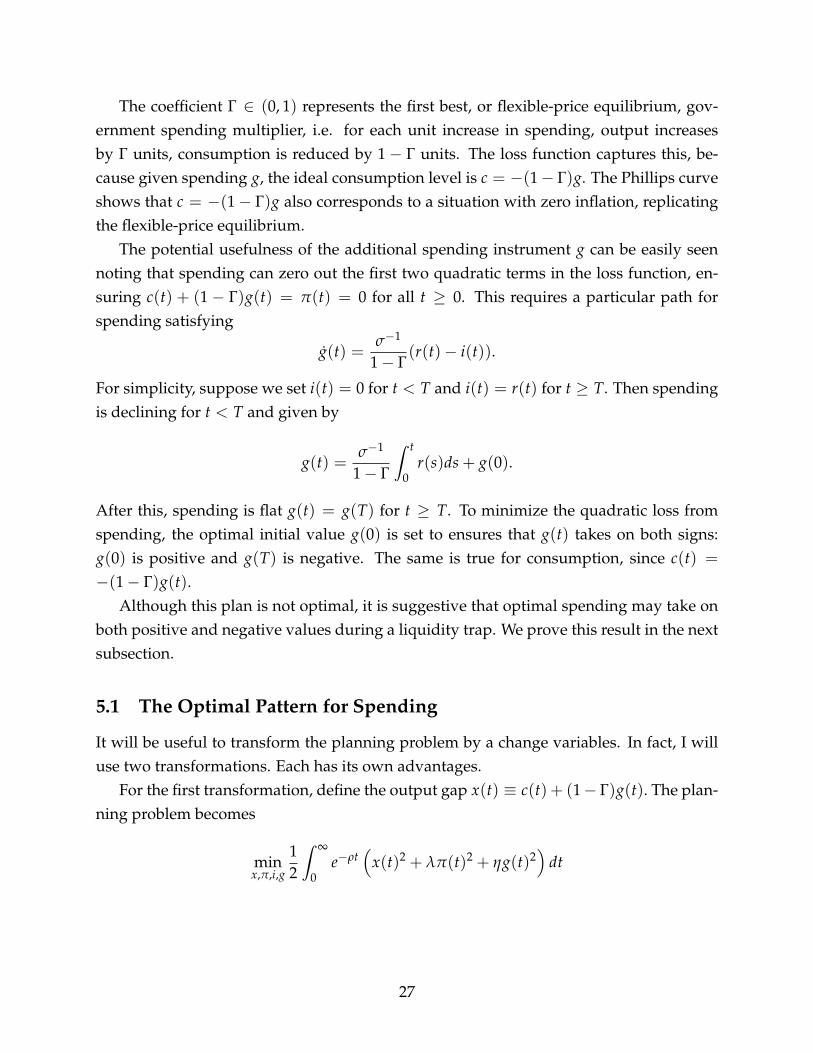
The coefficient Γ ∈ (0, 1) represents the first best, or flexible-price equilibrium, gov-ernment spending multiplier, i.e. for each unit increase in spending, output increasesby Γ units, consumption is reduced by 1− Γ units. The loss function captures this, be-cause given spending g, the ideal consumption level is c = −(1− Γ)g. The Phillips curveshows that c = −(1− Γ)g also corresponds to a situation with zero inflation, replicatingthe flexible-price equilibrium.

The potential usefulness of the additional spending instrument g can be easily seennoting that spending can zero out the first two quadratic terms in the loss function, en-suring c(t) + (1− Γ)g(t) = π(t) = 0 for all t ≥ 0. This requires a particular path forspending satisfying

g(t) =σ−1

1− Γ(r(t)− i(t)).

For simplicity, suppose we set i(t) = 0 for t < T and i(t) = r(t) for t ≥ T. Then spendingis declining for t < T and given by

g(t) =σ−1

1− Γ

ˆ t

0r(s)ds + g(0).

After this, spending is flat g(t) = g(T) for t ≥ T. To minimize the quadratic loss fromspending, the optimal initial value g(0) is set to ensures that g(t) takes on both signs:g(0) is positive and g(T) is negative. The same is true for consumption, since c(t) =

−(1− Γ)g(t).Although this plan is not optimal, it is suggestive that optimal spending may take on

both positive and negative values during a liquidity trap. We prove this result in the nextsubsection.

5.1 The Optimal Pattern for Spending

It will be useful to transform the planning problem by a change variables. In fact, I willuse two transformations. Each has its own advantages.

For the first transformation, define the output gap x(t) ≡ c(t) + (1− Γ)g(t). The plan-ning problem becomes

minx,π,i,g

12

ˆ ∞

0e−ρt

(x(t)2 + λπ(t)2 + ηg(t)2

)dt

27

subject to

x(t) = (1− Γ)g(t) + σ−1(i(t)− r(t)− π(t))

π(t) = ρπ(t)− κx(t)

i(t) ≥ 0

x(0), π(0) free.

This is an optimal control problem with i(t) and g(t) as controls and x and π as states.According to the objective, the ideal level of government spending, given the state vari-ables x(t) and π(t), is always zero, g(t). However, because spending also appears in theconstraints, it may help relax them. In particular, spending enters the constraint associ-ated with the consumer’s Euler equation. Indeed, the change in spending g(t) plays arole that is analogous to the nominal interest rate i(t). Unlike the latter, the former is notrestricted to being nonnegative.

Since government spending relaxes the Euler equation, it should be zero whenever thezero-bound constraint is not binding, which is the case whenever i(t) > 0. Conversely, ifthe zero-bound constraint binds and i(t) = 0 then government spending is not generallyzero. As the next proposition shows, spending is initially positive, then becomes negative,and finally returns to zero.

Proposition 6. Suppose the zero lower bound binds over the interval (t0, t1) and is slack in aneighborhood outside it. Then g(t0) > 0, g(t1) = 0 with g(t) < 0 for t < t1 in a neighborhoodof t1.

This result confirms the notion that government spending should be front loaded. Itmay seem surprising, however, that optimal spending takes on both positive and negativevalues. The intuition is as follows. Initially, higher spending helps compensate for thenegative consumption gap at the start of a liquidity trap. However, recall that optimalmonetary policy eventually engineers a consumption boom. If government spendingleans against the wind, we should expect lower spending. The next subsection refinesthis intuition by decomposing spending into an opportunistic and a stimulus component.

Figure 8 provides a numerical example, following the same parametrization used forthe example in Section 4, with the additional parameters Γ = 0.5 and η = .5. The figureshows both consumption and output. As we see from the figure consumption is not asaffected as output is in this case.

28

0 0 0 0.01 0.01 0.01

−0.04

−0.03

−0.02

−0.01

0

0.01

0.02

0.03

Figure 8: A numerical example. The optimum without spending (blue) vs. the optimumwith spending for output (red) and consumption (orange).

5.2 Opportunistic vs. Stimulus Spending

Even a shortsighted government that ignores dynamic general equilibrium effects on theprivate sector, finds reasons to increase government spending during a slump. When theeconomy is depressed, the wage, or shadow wage, is lowered. This provides a cheapopportunity for government consumption.

Based on this notion, I define an opportunistic component of spending, the level thatis optimal from a simple static, cost-benefit calculation. I then define the stimulus compo-nent of spending as the difference between actual spending and the opportunistic com-ponent. More precisely, given private consumption c, define opportunistic spending byminimizing the loss function,

g∗(c) ≡ arg maxg

{(c + (1− Γ)g)2 + ηg2

},

Define stimulus spending as the difference between actual and opportunistic spending,

g(t) ≡ g(t)− g∗(c(t)).

Note thatg∗(c) = −1− Γ

ηψc,

29

c + (1− Γ)g∗(c) = ψc,

with the constant ψ ≡ η/(η + (1− Γ)2) ∈ (0, 1). Thus, opportunistic spending leans

against the wind, ψ < 1, but does not close the gap, ψ > 0.Using these transformations, I rewrite the planning problem as

minx,π,i,g

12

ˆ ∞

0e−ρt

(c(t)2 + λπ(t)2 + η g(t)2

)dt

subject to

c(t) = σ−1(i(t)− r(t)− π(t))

π(t) = ρπ(t)− κ (ψc(t) + (1− Γ)g(t))

i(t) ≥ 0,

c(0), π(0) free.

where λ = λ/ψ and η = η/ψ2. According to the loss function, the ideal level of stimulusspending is zero. However, stimulus may help relax the Phillips curve constraint.

This problem is almost identical to the problem without spending. The only newoptimality condition is

g(t) =κ(1− Γ)

ηµπ(t). (4)

This gives a first result. Unlike total spending, stimulus spending is initially zero.

Proposition 7. Stimulus spending is always initially zero g(0) = 0.

Thus, total spending at the start of a liquidity trap is entirely opportunistic.18

To say more, note that the costate for the Phillips curve, unlike the costate for the Eulerequation, is not restricted to being nonnegative and the path it takes actually depends onparameters. Indeed, my main result for stimulus spending exploits this fact, providing abenchmark where stimulus spending is always zero.

Proposition 8. Suppose κσλ = 1. Then at an optimum g(t) = 0 for all t ≥ 0.

18Another implication of equation (4) is that stimulus spending, unlike total spending, may be nonzeroeven when the zero lower bound constraint is not currently binding and will never bind in the future. Thisoccurs whenever inflation is nonzero. Indeed, since total spending must be zero, stimulus spending mustbe canceling out opportunistic spending. This makes sense. If we have promised positive inflation, forexample, then we require a positive gap. Opportunistic spending would call for lower spending, but doingso would frustrate stimulating the promised inflation.

30

0 1 2 3

-0.02

0

0.02

0.04

0.06

0.08

Figure 9: Total spending (blue), opportunistic spending (green) and stimulus spending(red) for a numerical example. Both the case with monetary commitment (circles) anddiscretion (triangles) are shown.

Thus, under the conditions of the proposition, spending is entirely determined by itsopportunistic considerations. It is as if spending were chosen by a purely static cost-benefit calculation, with no regards for its dynamic general equilibrium impact on theeconomy. By implication, in this case government spending could be determined by anaive agency, lacking commitment, that performs a static cost-benefit calculation, ignor-ing the dynamic effects this has on the private sector.

Figure 9 displays the optimal paths for total, opportunistic and stimulus spending forour numerical example (with the same parameters as those behind Figure 8). Spendingstarts at 2% of output above it’s efficient level. It then falls at a steady state reachingalmost 2% below its efficient level of output. In this example, spending is virtually allopportunistic. Stimulus spending is virtually zero.

Away from this benchmark, numerical simulations show that stimulus starts at zero, ithas a sinusoidal shape, switching signs once. When κσλ > 1 it first becomes positive, thenturns negative, eventually asymptoting to zero from below; when κσλ < 1 the reversepattern obtains: first negative, then turns positive, eventually asymptoting to zero fromabove. In most cases, stimulus spending is a small component of total spending.

The results highlight that positive stimulus spending is just not a robust feature ofthe optimum for this model. Opportunistic spending does affect private consumption,

31

by affecting the path for inflation. In particular, by leaning against the wind, it promotesprice stability, mitigates both deflations and inflations. However, the effects are inciden-tal, in that they would be obtained by a policy maker choosing spending that ignoresthese effects.

6 Spending with Discretionary Monetary Policy

I now relax the assumption of full commitment and consider a mixed case, where mon-etary policy is discretionary, as in Section 3, while government spending is carried outwith commitment during the trap.

More specifically, consider the liquidity trap scenario, where r(t) < 0 for t < T andr(t) ≥ 0 for t ≥ T. Once the liquidity trap is over, monetary policy will implement theflexible-price equilibrium, so that c(t) + (1 − Γ)g(t) = 0 and π(t) = 0 for all t ≥ T.During the trap, the nominal interest rate is set to zero, i(t) = 0 for t < T. In contrast,the government spending can be credibly announced, at least for some time. I initiallyassume that spending after T is chosen with discretion, implying that g(t) = 0 for t ≥ T.I then consider the case with commitment on the entire path for government spending,for all t ∈ [0, ∞).

Government spending may be a powerful tool in this scenario. Absent spending, de-flation and depression prevail. But, as I argued above, spending can avoid both, achievinga zero output gap and inflation rate, c(t) + (1− Γ)g(t) = π(t) = 0 for all t ≥ 0. It does soby filling in the gap left by consumption. Of course, this simple plan is suboptimal. Next,I study optimal spending commitments.

6.1 Commitment to spending during the liquidity trap

The planning problem is essentially the same as before19 with the additional constraintthat

π(T) = c(T) = 0.

Once again the optimality condition gives

g(t) =κ(1− Γ)

ηµπ(t)

19Except that we may impose i(t) = 0 for t < T since this is chosen by the monetary authority. However,the optimum will also feature this interest rate path.

32

with the law of motion for the co-states as before. Thus, just as before, stimulus spendingis initially zero.

It is difficult to formally characterize the rest of the solution. I make progress by con-sidering small stimulus spending interventions, starting from spending. Specifically, con-sider appending the constraint

ˆ ∞

0e−ρtg(t)2dt ≤ G,

to the planning problem. Here G is a parameter. Setting G = 0 implies the no commit-ment outcome, without spending or stimulus, which involves deflation and depression.For G > 0 large enough the constraint no longer binds. The idea is to characterize theoptimum for small enough G > 0. This allows us to use the above formula for spending,with the costates evaluated at the original no spending and no discretion equilibrium.

Proposition 9. g(0) = 0. For small enough G > 0, g(t) ≥ 0 and is strictly increasing in t.Moreover, total spending is positive g(t) > 0 for all t ∈ [0, T).

Simulations support that this pattern generally carries over for the case where G ischosen freely. Figure 9 confirms this for the numerical example from the previous sec-tions. In this example, total spending is quite large and relatively flat. As opportunisticspending falls, stimulus spending rises and compensates.

6.2 Commitment to spending after the liquidity trap

I now relax the assumption that fiscal policy cannot commit past T. Thus, I now considera situation where spending is chosen for the entire future {g(t)}∞

t=0, allowing for g(t) 6= 0for t ≥ T.

This problem can be simplified by looking at the subproblem from t ≥ T. Clearly forany positive consumption c(T) > 0 the optimum calls for i(t) = 0 and g(t) = g(t) fort ∈ [T, T + ∆] and g(t) for t > T + ∆, where

g(t) = −(1− Γ)c(T) +σ−1

1− Γ

ˆ t

Tr(s)ds

and ∆ is defined so that g(T + ∆) = 0. Such a plan implies a tail cost

Ψ(c(T)) ≡ η

ˆ ∆

0e−ρsη g(T + s)2ds.

33

The planning problem can be rewritten as

minx,π,i,g

12

ˆ T

0e−ρt

(c(t)2 + λπ(t)2 + η g(t)2

)dt + e−ρTΨ(c(T))

subject to

c(t) = σ−1(i(t)− r(t)− π(t))

π(t) = ρπ(t)− κ (ψc(t) + (1− Γ)g(t))

i(t) ≥ 0,

π(T) = 0.

Under this formulation c(T) is a free variable, but the planner incurs a cost Ψ(c(T)). Thenew optimality condition (replacing c(T) = 0) is the transversality condition

µc(T) = Ψ′(c(T)).

A similar result applies in this case. For a small intervention, stimulus spending is pos-itive and increasing. Now, however, spending after the trap is negative, to promote aboom in consumption c(T), which helps raise the level of consumption at earlier dates,during the trap.

7 Conclusion

This paper has revisited monetary policy during a liquidity trap. The continuous timesetup up offers some distinct advantages in terms of the analysis and results that areobtained. Some of my results support the findings from prior work based on simulations.Pptimal monetary policy in the model is engineered to promote inflation and an outputboom. It does so, in part, by commiting to holding the nominal interest rate at zero for anextended period of time.

To the best of my knowledge, my results on government spending have no clear paral-lel in the literature. In particular, the decomposition between opportunistic and stimulusspending is novel and leads to unexpected results.

When both fiscal and monetary policy are coordinated, I find that optimal govern-ment spending starts at a positive level, but declines and become negative. However, Ishow that most of these dynamics are explained by a cost-benefit motive for spending,

34

which, by definition, ignores the effects this spending has on private consumption andinflation. At the model’s optimum, stimulus spending is always initially zero. Moreover,depending on parameters. stimulus may be identically zero throughout or deviate fromzero changing signs. However, simulations show stimulus spending playing a modestrole.

This situation can be very different when monetary policy is suboptimal due to thelack of commitment. In this case, the model’s optimal policy calls for positive and in-creasing stimulus spending during the trap and lower spending after the trap.

References

Adam, Klaus and Roberto M. Billi, “Optimal Monetary Policy under Commitment witha Zero Bound on Nominal Interest Rates,” Journal of Money, Credit and Banking, October2006, 38 (7), 1877–1905.

Blanchard, Olivier, Giovanni Dell’Ariccia, and Paolo Mauro, “Rethinking Macroeco-nomic Policy,” Journal of Money, Credit and Banking, 09 2010, 42 (s1), 199–215.

Christiano, Lawrence, Martin Eichenbaum, and Sergio Rebelo, “When is the govern-ment spending multiplier large?,” Journal of Political Economy, February 2011, 119 (1).

Clarida, Richard, Jordi Gali, and Mark Gertler, “The Science of Monetary Policy: A NewKeynesian Perspective,” Journal of Economic Literature, December 1999, 37 (4), 1661–1707.

Eggertsson, Gauti B., “Real Government Spending in a Liquidity Trap,” 2001.

, “The Deflation Bias and Committing to Being Irresponsible,” Journal of Money, Creditand Banking, March 2006, 38 (2), 283–321.

, “What Fiscal Policy is Effective at Zero Interest Rates?,” in “NBER MacroconomicsAnnual 2010, Volume 25” NBER Chapters December 2011, pp. 59–112.

and Michael Woodford, “The Zero Bound on Interest Rates and Optimal MonetaryPolicy,” Brookings Papers on Economic Activity, 2003, 34 (2003-1), 139–235.

Galí, Jordi, Monetary Policy, Inflation, and the Business Cycle: An Introduction to the NewKeynesian Framework, Princeton University Press, 2008.

35

Jung, Taehun, Yuki Teranishi, and Tsutomu Watanabe, “Optimal Monetary Policy at theZero-Interest-Rate Bound,” Journal of Money, Credit and Banking, October 2005, 37 (5),813–35.

Krugman, Paul R., “It’s Baaack: Japan’s Slump and the Return of the Liquidity Trap,”Brookings Papers on Economic Activity, 1998, 29 (1998-2), 137–206.

Long, James Bradford De and Lawrence H. Summers, “Is Increased Price FlexibilityStabilizing?,” American Economic Review, December 1986, 76 (5), 1031–44.

Summers, Lawrence, “Panel discussion: price stability ; How should long-term monetarypolicy be determined?,” Proceedings, Aug. 1991, 23 (3, part 2: Price Stability), 625–631.

Woodford, Michael, Interest and Prices: Foundations of a Theory of Monetary Policy, Prince-ton University Press, 2003.

, “Simple Analytics of the Government Expenditure Multiplier,” American EconomicJournal: Macroeconomics, January 2011, 3 (1), 1–35.

A Proof of Proposition 1

Recall that π(t) = x(t) = 0 for t ≥ T. In integral form the equilibrium conditions fort < T are

x(t) =ˆ T

tσ−1(r(s) + π(s))ds,

π(t) = κ

ˆ T

te−ρ(s−t)x(s)ds.

Substituting inflation π(t) we can write this as a single condition for the output path{x(t)}

x(t) = σ−1ˆ T

t

(r(s) + κ

ˆ T

se−ρ(z−s)x(z)dz

)ds.

Define the operator associated with the right hand side of this expression:

T[x](t) = σ−1ˆ T

t

(r(s) + κ

ˆ T

se−ρ(z−s)x(z)dz

)ds = a(t) + κ

ˆ T

tm(z− t)x(z)dz

36

with a(t) ≡ σ−1 ´ Tt r(z)dz and m(s) ≡ (σρ)−1(1 − e−ρs), note that m is nonnegative,

strictly increasing, with m(0) = 0 and lims→∞ m(s) = M ≡ (σρ)−1 > 0.The operator T maps the space of continuous functions on (−∞, T] onto itself. An

equilibrium x∗ is a fixed point T[x∗] = x∗. Since an equilibrium represents a solution toan initial value problem for a linear ordinary differential equation, there is a unique fixedpoint x∗. The T operator is linear and monotone (since m ≥ 0), so that if xa ≥ xb thenT[xa] ≥ T[xb].

Fix an interval [t, T]. Although T is not a contraction, starting from any continuousfunction x0 that is bounded on [t, T] and defining xn ≡ Tn[x0] we obtain a sequence thatconverges uniformly on [t, T] to the unique fixed point xn → x∗. To prove this claim, notethat since |x0(t)| ≤ B and |r(t)| ≤ R then

|x1(t)− x0(t)| ≤ |a(t)|+ κ

ˆ T

tm(z− t) |x0(t)| ≤

(R

κM+ B

)κM|T − t|.

In turn

|x2(t)− x1(t)| = |T[x1](t)− T[x0](t)| ≤ κ

ˆ T

tm(z− t) |x1(z)− x0(z)| dz

≤ κMˆ T

t|x1(z)− x0(z)| dz ≤

(R

κM+ B

)(κM)2 |T − t|2

2.

By induction it follows that

|xn(t)− xn−1(t)| ≤(

RκM

+ B)(κM)n |T − t|n

n!.

It follows that∞

∑n=1|xn − xn−1(t)| ≤

(R

κM+ B

)eκM|T−t|.

As a consequence for any m ≥ n

|xn − xm(t)| ≤m

∑j=n+1

|xj − xj−1(t)| ≤∞

∑j=n+1

|xj − xj−1(t)|

Since the right hand converges to zero as n → ∞, for any ε > 0 and t′ < T there exists anN such that for all n, m ≥ N we have

|xn(t)− xm(t)| ≤ ε

37

for all t ≥ t′. Thus, {xn} is a Cauchy sequence on a complete metric space, implying thatxn → x∗ where x∗ is a bounded function. Since the operator T is continuous it followsthat x∗ is a fixed point x∗ = T[x∗].

Note that starting from the zero function x0(t) = 0 for all t we obtain x1(t) = a(t) < 0for t < T. Since the operator T is monotone, the sequence {xn} is decreasing x0 ≥ x1 ≥· · · ≥ xn ≥ · · · Thus, x∗(t) < x1(t) < 0 for all t < T. This implies π∗(t) < 0 for t < T.

Next I establish that both inflation and output x∗(t) and π∗(t) are monotone. Notethat ∂

∂t T[x](t) = a′(t) −´ T

t m′(z − t)x(z)dz. Since a′(t) = −σ−1r(t) > 0 and x∗(t) < 0for t < T we have that T[x∗](t) = x∗(t) is strictly increasing in t for t < T. Likewise,differentiating we find π(t) = ρκ

´ ∞0 e−ρz(x(t + s)− x(t))ds, which implies π∗(t) > 0 for

t < T given that x∗(t + s) ≥ x∗(t) with strict inequality for s > 0 and t + s ≤ T.Finally note that

x∗(t; T) = σ−1ˆ T

t(r(s; T)− π∗(s; T))ds ≤ σ−1

ˆ T

tr(s; T)ds

and since´ T

0 r(s; T)ds → −∞ as T → ∞ it follows that´ T

t r(s; T)ds → −∞, implyingx∗(t; T)→ −∞ for t < T. Using that x∗(t, T) ≤ 0, this implies that

π∗(t, T) = κ

ˆ ∞

te−ρ(s−t)x∗(s; T)ds ≤ κ

ˆ t+1

te−ρ(s−t)x∗(s; T)ds

≤ κx∗(t + 1; T)ˆ t+1

te−ρ(s−t)ds

As T → ∞ we have that x∗(t + 1; T)→ −∞, so it follows that π∗(t; T)→ −∞ for any t.

B Proof of Proposition 2

Consider two values κ0 < κ1 with associated equilibria x∗0 and x∗1 . Let T[·; κ] be the op-erator defined in the proof of Proposition 1 associated with κ. Define the sequence xn =

Tn[x∗0 ; κ1]. Since x∗0(t) < 0 for t < T, it follows that x1(t) = T[x∗0 ; κ1] < T[x∗0 ; κ0] = x0(t)for t < T. Since the operator T[·; κ0] is monotone, this implies that {xn} is a decliningsequence. Since the sequence converges to x∗1 . This proves that x∗0(t) > x1(t) > · · · >xn(t) > · · · > x∗1(t) for t < T. This implies that π∗1(t) < π∗0(t) for t < T.

To prove the limit result as κ1 → ∞ it suffices to show that T[x∗0 ; κ1](t) → −∞ for all

38

t < T. This follows from

T[x∗0 ; κ1](t) = a(t) + κ

ˆ T

tm(z− t)x∗0(z)dz ≤ κ1

ˆ T

tm(z− t)a(z)dz

and the result follows from the fact that´ T

t m(z− t)a(z)dz < 0 for all t < T. The sameimplication for π∗(t; κ) then follows.

The following estimate for the loss function

L ≥ˆ ∞

0e−ρtx(t)2dt ≥

ˆ T/2

0e−ρtx(t; κ)2dt ≥ x(T/2; κ)2

ˆ T/2

0e−ρtdt

where I have used that x is nonpositive and increasing. The result then follows sincex(T/2; κ)→ −∞.

C Proof of Proposition 3

Suppose i(t) > 0 for t ∈ (t′, t′ + ε) with ε > 0. Then it must be that µ(t) = µ(t) = 0 fort ∈ [t′, t′ + ε). However, whenever µx(t) ≤ 0 we have

˙µx(t) = −x(t) + κµπ(t) + ρµx(t)

≤ −σ−1(i(t)− r(t)− π(t))− κλπ(t)

= σ−1 (I∗(π(t), t)− i(t))

where I have used that µx(t) ≥ 0.It follows that if I∗(π(t), t) < 0 for t ∈ (t′ − ε, t′) then ˙µx(t) < 0. Since µx(t′) = 0 this

implies µx(t) > 0 for t ∈ (t′ − ε, t′). Given that µx(t′) = 0 this then implies that µx(t) < 0for t ∈ (t′ − ε, t′), a contradiction with the optimality conditions.

D Proof of Proposition 4

The initial conditions require µx(0) = µπ(0) = 0. The non-negativity requirement for µx

then requires µx(0) = −x(0) ≥ 0, implying x(0) ≤ 0.To establish that inflation must be positive at some point, consider the perturbation

x(t, ε) = x(t) + ε and

π(t, ε) = κ

ˆ ∞

0e−ρsx(t + s, ε)ds = κ

ˆ ∞

0e−ρsx(t + s)ds + κ

ˆ ∞

0e−ρsεds = π(t) +

κ

ρε.

39

Note that the perturbation is feasible for all ε > 0 since higher inflation relaxes the ZLBconstraint σx(t) ≥ −r(t)− π(t). In terms of the loss function

L(ε) =12

ˆ ∞

0e−ρt

(x(t, ε)2 + λπ(t, ε)2

)dt

we have

L′(0) =ˆ ∞

0e−ρt

(x(t) + λ

κ

ρπ(t)

)dt =

1κ

π(0) + λκ

ρ

ˆ ∞

0e−ρtπ(t)dt ≤ 0.

Hence, negative inflation π(t) ≤ 0 for all t ≥ 0 with strict inequality over some range,implies L′(0) < 0, a contradiction with optimality.

Now suppose κσλ = 1. Suppose (π(t), x(t)) satisfy the ODE system (1a)–(1b) withi(t) = 0 for t ∈ [0, T] with T > T. Now set µπ(t) = 0 and define µx(t) = σλπ(t) so that

µπ = 0 = −λπ + σ−1µx

µx(t) = σλ(ρπ(t)− κx(t)) = −x(t) + ρσλπ(t)

are both satisfied. It follows that (π(t), x(t))t∈[0,T] together with π(t) = x(t) = 0 for t > Tis optimal if and only if π(t) ≥ 0 and π(0) = π(T) = 0 and x(T) = 0.

To establish that x(t) must be positive for some t ≥ 0, proceed by contradiction. Sup-pose x(t) ≤ 0 for all t ≥ 0. This implies that π(t) ≤ 0 for all t ≥ 0, a contradiction.

40