Managerial Statistics

1 | P a g e

COURSE DOCKET*

SUBJECT: MANAGERIAL STATISTICS

PGDM TERM – I

FACULTY: ROHIT R. MUTKEKAR

*Disclaimer: Course Docket will help you for quick reference and provides fundamental inputs,

hence cannot be substitute for text book/reference books

2 | P a g e

Course Docket

Subject: Managerial Statistics

Correlation Analysis

Introduction

Classification Correlation

o Positive/Negative/Zero Correlation

o Simple/Multiple/Partial Correlation

o Linear/Non-Linear Correlation

Degree of Correlation

Methods to determine Simple Correlation

o Scatter Diagram Method

o Karl Pearson Method

o Spearmen’s Rank Correlation Method

Properties of Correlation

o Examples on Simple Correlation Analysis

1. The following data provides details regarding sales and net profit for some of the top auto

makers during the quarter July-September 2006. Find the co-efficient of correlation using

an appropriate method and interpret the result.

Company Average Sales (X)

(Rs. Crores)

Average Profit (Y)

(Rs. Crores)

Tata Motors 6484.8 466

Hero Honda 2196.5 224.2

Bajaj Auto 2444.7 345.4

TVS Motor 1032.9 35.1

Bharat Forge 461.6 63.4

Ashok Leyland 1635.8 94.7

M & M 2365.5 200.6

Maruti Udyog 3426.5 315.7

Source: Economic Times, 11th October, 2006

3 | P a g e

Coefficient of Determination (r2)

2. The following are the monthly figures of advertising expenditures and sales of a firm. It is

generally found that the advertising expenditures has an impact on sales. Determine the

co-efficient of correlation for the data provided using rank correlation method.

Month Adv Expenditure (Rs’ 000) Sales (Rs’000)

Jan 50 1200

Feb 60 1500

March 90 1600

April 70 2000

May 120 2200

June 150 2400

July 140 2500

Aug 160 2600

Sept 190 2800

Oct 170 2900

Nov 200 3100

Dec 250 3900

3. Find the co-efficient of correlation between the two kinds of assessment of postgraduate

students’ performance in a college using the rank correlation method.

Name

Assessment Marks

Internal External

A 51 50

B 63 72

C 73 74

D 46 50

E 50 58

F 60 66

G 47 50

H 36 30

I 60 35

4 | P a g e

Statistical Significance of Correlation

o For Karl Pearson’s Method

o For Spearmen’s Rank Method

Assignment 1

1. Calculate the co-efficient of correlation for the original data given in Example 1 using

Karl Pearson’s method. Determine the amount of variation in the result as compared to

the round of values. What can you conclude from this exercise?

2. A group of students of management programme at a certain institute were selected at

random. Their IQ and the marks obtained by them in the paper on decision science were

recorded. The details are as follows –

IQ Marks

Scored

120 85

110 80

130 90

115 88

125 92

120 87

Calculate co-efficient of correlation using Karl Pearson’s and Spearmen’s Rank Method

and test for statistical significance in both the cases at 5% l.o.s.

3. Given below is the data about revenues and profit after tax for the quarter July-

September 2007 of some cement companies. Compute the co-efficient of correlation

using appropriate method and interpret the result. Also test the statistical significance at

1%.

Company Revenues

(Rs Crores)

Profit after Tax

(Rs Crores)

ACC 13 2.5

Ambuja 21 3.2

Ultratech 10 2.6

Shree 9 1.4

India 5 1.1

Bagalkot 3 0.8

5 | P a g e

Regression Analysis

Introduction

Types of Regression

o Simple Regression

o Multiple Regression

Simple Linear Regression Analysis using Least Squares Method

o Examples on Simple Regression Analysis using Least Squares Method

1. A group of students of management programme at a certain institute were selected at

random. Their IQ and the marks obtained by them in the paper on decision science were

recorded. The details are as follows –

IQ Marks

Scored

120 85

110 80

130 90

115 88

125 92

120 87

Fit a regression equation and interpret the result so obtained.

2. A national level organization wishes to prepare a manpower plan based on the ever

growing sales offices in the country. Data pertaining to manpower and the number of sales

offices for previous is given below-

Fit a regression model for the given data and estimate the manpower required if the

organization targets to have 43 sales offices at the end of 2015.

Manpower Sales Offices

370 22

386 25

443 28

499 31

528 33

616 38

6 | P a g e

3. The following data is relates to training and performance of salesmen employed in a

company.

Fit a regression model and determine the weekly sales that is likely to be attained by a

salesman who is given 16 hours of training.

Regression Co-efficients

Standard Error of Estimate

Co-efficient of Determination

How good is the Regression?

Multiple Regression Analysis

Introduction

General form of Multiple Regression Model

Standard Error for Multiple Regression Model

o Examples on Multiple Regression Analysis

1. Fit a regression model for the following data and interpret the result

Sales

(Rs.Lakh)

Adv Expenses

(Rs’000)

Selling

Offices

100 40 10

80 30 10

60 20 7

120 50 15

150 60 20

90 40 12

70 20 8

130 60 14

Training (hrs.) Performance(Avg weekly sales)

20 44

5 22

10 25

13 32

12 27

7 | P a g e

2. The owner of a chain of the stores wishes to forecast net profit with the help of next years

projected sales of food and non-food items. The data about the current year’s sales of food

items, sales of non-food items as also net profit for all the ten stores are available as follows-

Fit a regression model and interpret the result.

Adjusted Coefficient of Determination

Multicollinearity in Multiple Regression

Selection of Independent Variables in a Regression Model

Assignment 2

1. For the following data fit regression equations of-

i. Net Profit on Net Sales

ii. P/E ratio on Net Sales

For the group of these companies

Name of the

Company

Net Sales(Rs. Cr)

(Sept, 2005)

Net Profit (Rs. Cr)

(Sept, 2005)

P/E Ratio

(31st Oct, 2005)

Infosys 7836 2170.9 32

Wipro 8051 1831.4 30

Bharti 8211 1655.8 31

Hero Honda 9771 1753.5 128

ITC 8086 868.4 16

Satyam 8422 2351.3 20

HDFC 3996 844.8 23

Tata Motors 18368 1314.9 14

Siemens 2753 254.7 38

Interpret the result in terms of standard error, R2 and significance of regression model.

Net Profit

(Rs.Cr)

Sales of Food

Items (Rs.Cr)

Sales of Non-Food Items

(Rs.Cr)

5.6 20 5

4.7 15 5

5.4 18 6

5.5 20 5

5.1 16 6

6.8 25 6

5.8 22 4

8.2 30 7

5.8 24 3

6.2 25 4

8 | P a g e

2. A company wants to assess the impact of R&D expenditure (Rs. Cr) on Annual profits

(Rs. Cr). The following table give information for the past 8 years.

Year R&D expenditure Annual profits

2006 9 45

2007 7 42

2008 5 41

2009 10 60

2010 4 30

2011 5 34

2012 3 25

2013 2 20

Fit a regression model. Interpret the result in terms of standard error, R2 and significance

of regression model.

3. Ashwin, owner of a business unit, is concerned about the sales pattern of his product. He

realizes that there are many factors that might help explain sales, but believes that

advertising and prices are major determinants. He has collected data from the past

records which are as follows-

Sales (unit sold) 37 65 75 87 22 29

Advertising (No of ads) 07 10 14 17 13 10

Price (Rs’000) 129 115 140 130 145 140

Fit a regression model. Interpret the result in terms of standard error, R2 and significance

of regression model.

9 | P a g e

Introduction to Statistical Inference

Introduction

Parameter

Statistic

Sample Space

Sampling Distribution

Standard Error

Testing of Hypothesis

Hypothesis

Statistical Hypothesis

o Simple Hypothesis

o Composite Hypothesis

Null Hypothesis

Alternative Hypothesis

Test Statistic

Null Distribution

Critical (Rejection) Region

Acceptance Region

Errors in Hypothesis Testing

Actual Fact Decision based on

sample

observation

Inference Error

H0 is true Accept H0 Correct Decision --

H0 is true Reject H0 Incorrect Decision Type I

H0 is false Accept H0 Incorrect Decision Type II

H0 is false Reject H0 Correct Decision --

Type I Error

Type II Error

Size of the test (Level of Significance)

Power of the test

One Tail Test

Two Tail Test

Procedure in Hypothesis Testing

o Formulation of Hypothesis

o Set up a suitable significance level

o Select the test criterion

o Computation

o Decision making

10 | P a g e

Large Sample Tests (Z Tests)

Z-Test for Single Mean (Theory)

Here the null hypothesis is given by,

H0: 𝜇 = 𝜇0

For the above null hypothesis, we may have any one of the following alternatives,

a) H1: 𝜇 ≠ 𝜇0 (Two tail test)

b) H1: 𝜇 > 𝜇0 (One tail test – Upper)

c) H1: 𝜇 < 𝜇0 (One tail test – Lower)

Now the test statistic under H0 is given by,

𝑍𝑜𝑏𝑠 =�̅� − 𝜇0

𝜎

√𝑛

~ 𝑁(0,1)

�̅� denotes sample mean

𝜇0 denotes standard value at which the population mean 𝜇 is tested

𝜎 denotes population standard deviation

𝑛 denotes sample size

(Noted: If 𝝈 is not specified then we need to use the sample standard deviation‘s’)

Decision Making

a) If we are testing H0: 𝜇 = 𝜇0 vs H1: 𝜇 ≠ 𝜇0 at α level of significance, then we can reject

H0 if 𝑍𝑜𝑏𝑠 is lying outside the interval (−𝑍α2⁄ , +𝑍α

2⁄ )

b) If we are testing H0: 𝜇 = 𝜇0 vs H1: 𝜇 > 𝜇0 at α level of significance, then we can reject

H0 if 𝑍𝑜𝑏𝑠 > 𝑍α

c) If we are testing H0: 𝜇 = 𝜇0 vs H1: 𝜇 < 𝜇0 at α level of significance, then we can reject

H0 if 𝑍𝑜𝑏𝑠 < - 𝑍α

Here 𝑍α and 𝑍α2⁄ are Normal Table (Z) values at α level of significance

Z-Test for Two Means (Theory)


H0: 𝜇1 = 𝜇2


a) H1: 𝜇1 ≠ 𝜇2 (Two tail test)

b) H1: 𝜇1 > 𝜇2 (One tail test – Upper)

c) H1: 𝜇1 < 𝜇2 (One tail test – Lower)


𝑍𝑜𝑏𝑠 =�̅�1 − �̅�2

√𝜎1

2

𝑛1+

𝜎22

𝑛2

~ 𝑁(0,1)

11 | P a g e

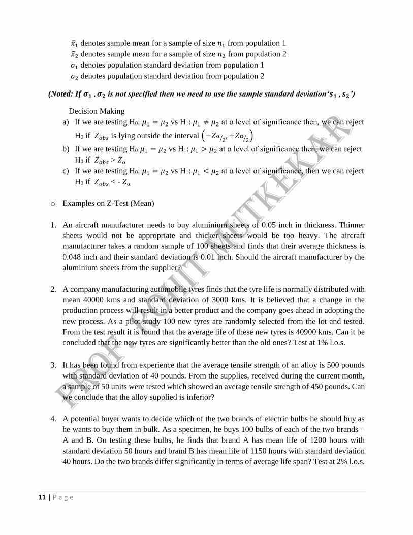
�̅�1 denotes sample mean for a sample of size 𝑛1 from population 1


𝜎1 denotes population standard deviation from population 1

𝜎2 denotes population standard deviation from population 2

(Noted: If 𝝈𝟏 , 𝝈𝟐 is not specified then we need to use the sample standard deviation‘𝒔𝟏 , 𝒔𝟐’)

Decision Making

a) If we are testing H0: 𝜇1 = 𝜇2 vs H1: 𝜇1 ≠ 𝜇2 at α level of significance then, we can reject


2⁄ )

b) If we are testing H0:𝜇1 = 𝜇2 vs H1: 𝜇1 > 𝜇2 at α level of significance then, we can reject


c) If we are testing H0: 𝜇1 = 𝜇2 vs H1: 𝜇1 < 𝜇2 at α level of significance, then we can reject


o Examples on Z-Test (Mean)

1. An aircraft manufacturer needs to buy aluminium sheets of 0.05 inch in thickness. Thinner

sheets would not be appropriate and thicker sheets would be too heavy. The aircraft

manufacturer takes a random sample of 100 sheets and finds that their average thickness is

0.048 inch and their standard deviation is 0.01 inch. Should the aircraft manufacturer by the

aluminium sheets from the supplier?

2. A company manufacturing automobile tyres finds that the tyre life is normally distributed with

mean 40000 kms and standard deviation of 3000 kms. It is believed that a change in the

production process will result in a better product and the company goes ahead in adopting the

new process. As a pilot study 100 new tyres are randomly selected from the lot and tested.

From the test result it is found that the average life of these new tyres is 40900 kms. Can it be

concluded that the new tyres are significantly better than the old ones? Test at 1% l.o.s.

3. It has been found from experience that the average tensile strength of an alloy is 500 pounds

with standard deviation of 40 pounds. From the supplies, received during the current month,

a sample of 50 units were tested which showed an average tensile strength of 450 pounds. Can

we conclude that the alloy supplied is inferior?

4. A potential buyer wants to decide which of the two brands of electric bulbs he should buy as

he wants to buy them in bulk. As a specimen, he buys 100 bulbs of each of the two brands –

A and B. On testing these bulbs, he finds that brand A has mean life of 1200 hours with

standard deviation 50 hours and brand B has mean life of 1150 hours with standard deviation

40 hours. Do the two brands differ significantly in terms of average life span? Test at 2% l.o.s.

12 | P a g e

5. An automobile company is interested in testing the average mileage given by one of the car

brand in two different cities i.e. Delhi and Mumbai. The company surveyed 100 car owners in

Delhi and found the average mileage is 12 kms and it surveyed 150 owners in Mumbai and

found the average mileage is 12.5 kms. The standard deviation for mileage of this brand of car

is known to be 0.9 kms. Can we conclude that the cars gives better average in Mumbai as

compared to Delhi? Test at 5% l.o.s.

Examples on Z test using MS Excel

1. A business school in its advertisement claims that the average salary of its graduates in a

particular lean year is at par with the average salaries offered at the top five business schools.

A sample of 35 graduates, from the business school whose claim was to be verified, was taken

at random. The average salary offered at the top five business schools in that year was given

as Rs.750000. Test the validity of the claim.

Student Salary(000's)

1 750

2 600

3 600

4 650

5 700

6 780

7 860

8 810

9 780

10 670

11 690

12 550

13 610

14 715

15 755

16 770

17 680

18 670

19 740

20 760

21 775

22 845

23 870

24 640

25 690

26 715

27 630

28 685

29 780

30 635

13 | P a g e

31 770

32 665

33 780

34 550

35 620

2. A large organization produces electric light bulbs in each of its two factories (A and B). It is

suspected that the quality of production from factory A is better than factory B. To test this

assertion the organization collets samples from factory A and B, and measures how long each

light bulb works (in hours) before it fails (relevant data is given below). Both population

variances are known i.e. Var(A)=52783 and Var(B)=61560. Test the assertion at 5% l.o.s.

Factory A Factory B

900 1052

1276 947

1421 886

1014 788

1246 1188

1507 928

975 983

1177 970

1246 766

875 1369

816 737

983 1114

1119 354

988 1347

1137 1062

1227 756

858 1052

941 754

1299 990

1110 950

929 783

843 816

1156 658

867 504

1454 1076

1403 500

1165 1025

1653 649

1288 1166

1187 498

945

1002

14 | P a g e

Z-Test for Single Proportion (Theory)


H0: 𝑃 = 𝑃0


a) H1: 𝑃 ≠ 𝑃0 (Two tail test)

b) H1: 𝑃 > 𝑃0 (One tail test – Upper)

c) H1: 𝑃 < 𝑃0 (One tail test – Lower)


𝑍𝑜𝑏𝑠 =𝑝 − 𝑃0

√𝑃0. 𝑄0

𝑛

~ 𝑁(0,1)

𝑝 denotes sample proportion

𝑃0 standard value at which the population proportion P is tested

𝑄0 = 1 − 𝑃0


Decision Making

a) If we are testing H0: 𝑃 = 𝑃0 vs H1: 𝑃 ≠ 𝑃0 at α level of significance then we can reject


2⁄ )

b) If we are testing H0: 𝑃 = 𝑃0 vs H1: 𝑃 > 𝑃0 at α level of significance then we can reject


c) If we are testing H0: 𝑃 = 𝑃0 vs H1: 𝑃 < 𝑃0 at α level of significance then we can reject


Z-Test for Two Proportions (Theory)


H0: 𝑃1 = 𝑃2


a) H1: 𝑃1 ≠ 𝑃2 (Two tail test)

b) H1: 𝑃1 > 𝑃2 (One tail test – Upper)

c) H1: 𝑃1 < 𝜇2 (One tail test – Lower)


𝑍𝑜𝑏𝑠 =𝑝1 − 𝑝2

√𝑃.̂ 𝑄.̂ (1𝑛1

+1

𝑛2)

~ 𝑁(0,1)

Where �̂� = 𝑛1𝑝1+𝑛2𝑝2

𝑛1+𝑛2 and �̂� = 1 − �̂�

𝑝1 denotes sample proportion for a sample of size 𝑛1 from population 1

𝑝2 denotes sample proportion for a sample of size 𝑛2 from population 2

𝑃1 denotes population proportion for population 1

𝑃2 denotes population proportion for population 2

15 | P a g e

Decision Making

a) If we are testing H0: 𝑃1 = 𝑃2 vs H1: 𝑃1 ≠ 𝑃2 at α level of significance then we can reject


2⁄ )

b) If we are testing H0:𝑃1 = 𝑃2 vs H1: 𝑃1 > 𝑃2 at α level of significance then we can reject


c) If we are testing H0: 𝑃1 = 𝑃2 vs H1: 𝑃1 < 𝑃2 at α level of significance then we can reject


o Examples on Z-Test (Proportion)

1. It is known from the past data that 10% of the families in a certain locality subscribe to a

periodical called Outlook. Of late, there has been some apprehension that the subscription rate

has declined. In order to test whether there has been a decline, a random sample of 100 families

were surveyed from the locality and it was found that 7 families did subscribe for Outlook.

Can it be concluded that the subscription rate has really declined? Test at 5% l.o.s.

2. The owner of a departmental stores claims that majority of his customers use credit/debit card

as their payment option. To verify the claim made, 800 customers were randomly observed

during the given time and it was found that 420 made payment using credit/debit card. Discuss

whether the information supports the view and test the same at 1% l.o.s.

3. A cable TV operator claims that 50% of the homes in a city have opted for his services. Before

sponsoring advertisements on the local cable channel, a firm conducted a survey and found

that 280 homes out of 600 to have cable TV service provided by the operator. On this basis of

the data can we accept the claim made by the cable operator? Test at 1% l.o.s.

4. A company is considering two different ads for promotion of a new product. After watching

both the ads, the management believes that advertisement A is more effective than

advertisement B. Two test market areas with virtually identical consumer characteristics are

selected. Advertisement A is used in one area and B in another. In a random sample of 60

customers who saw advertisement A, 18 tried the product and similarly a random sample of

100 customers who saw advertisement B, 22 tried the product. Does this indicate that

advertisement A is more effective than advertisement B, test at 5% l.o.s.

5. You obtain a large number of components to an identical specification from 2 sources. You

notice that some of the components are from the suppliers own plant at Pune and some are

from the plant at Bangalore. You would like to know whether the proportion of defective

components are the same or there is a difference between them. For this, you take a random

sample of 600 components from each plant and find the sample proportion of defective

components as 0.015 and 0.017 respectively. Test at 1% l.o.s., whether the proportion of

defectives differ significantly with respect to these two plants.

16 | P a g e

Small Sample Tests (t Tests)

t-Test for Single Mean (Theory)


H0: 𝜇 = 𝜇0


a) H1: 𝜇 ≠ 𝜇0 (Two tail test)

b) H1: 𝜇 > 𝜇0 (One tail test – Upper)

c) H1: 𝜇 < 𝜇0 (One tail test – Lower)


𝑡𝑜𝑏𝑠 =�̅� − 𝜇0

𝑠

√𝑛 − 1

~ 𝑡(𝑛 − 1)degree of freedom

�̅� denotes sample mean

𝜇0 denotes standard value at which the population mean 𝜇 is tested

𝑠 denotes sample standard deviation


Decision Making

a) If we are testing H0: 𝜇 = 𝜇0 vs H1: 𝜇 ≠ 𝜇0 at α level of significance then, we can reject

H0 if 𝑡𝑜𝑏𝑠 is lying outside the interval (−𝑡α2⁄ , +𝑡α

2⁄ )

b) If we are testing H0: 𝜇 = 𝜇0 vs H1: 𝜇 > 𝜇0 at α level of significance then, we can reject

H0 if 𝑡𝑜𝑏𝑠 > 𝑡α

c) If we are testing H0: 𝜇 = 𝜇0 vs H1: 𝜇 < 𝜇0 at α level of significance then, we can reject

H0 if 𝑡𝑜𝑏𝑠 < - 𝑡α

Here 𝑡α and 𝑡α2⁄ are t distribution table values at α level of significance

t-Test for Two Means (Theory)


H0: 𝜇1 = 𝜇2


a) H1: 𝜇1 ≠ 𝜇2 (Two tail test)

b) H1: 𝜇1 > 𝜇2 (One tail test – Upper)

c) H1: 𝜇1 < 𝜇2 (One tail test – Lower)


𝑡𝑜𝑏𝑠 =�̅�1 − �̅�2

√𝑛1𝑠1

2 + 𝑛2𝑠22

𝑛1 + 𝑛2 − 2 . (𝑛1 + 𝑛2

𝑛1. 𝑛2)

~ 𝑡(𝑛1 + 𝑛2 − 2)degree of freedom

17 | P a g e



𝑠1 denotes sample standard deviation for a sample of size 𝑛1 from population 1

𝑠2 denotes sample standard deviation for a sample of size 𝑛2 from population 2

Decision Making

a) If we are testing H0: 𝜇1 = 𝜇2 vs H1: 𝜇1 ≠ 𝜇2 at α level of significance then we can reject

H0 if 𝑡𝑜𝑏𝑠 is lying outside the interval (−𝑡α2⁄ , +𝑡α

2⁄ )

b) If we are testing H0:𝜇1 = 𝜇2 vs H1: 𝜇1 > 𝜇2 at α level of significance then we can reject


c) If we are testing H0: 𝜇1 = 𝜇2 vs H1: 𝜇1 < 𝜇2 at α level of significance then we can reject


o Examples on t-Test (Mean)

1. The mean nicotine content of a brand of cigarette is 20.0 mgs. A new process is proposed to

lower the nicotine content without affecting the quality. To test the new process, 16 cigarettes

are selected at random from the output obtained from the test plant. The sample mean nicotine

content is found to be 18.5 mg with standard deviation of 2 mg. Is the claim for the new

process justified? Test at 5% l.o.s.

2. A car manufacturer claims that its new car gives a mileage of atleast 15 kms/litre of petrol. A

sample of 10 cars is taken at random, and their mileage recorded are as follows:

16.2, 15.7, 16.3, 16.0, 15.8, 15.7, 15.6, 15.6, 15.7, 15.4

Is there any statistical evidence to support the claim of the manufacturer about the mileage?

3. A local car dealer wants to know if the purchasing habits of a buyer buying extras have

changed. He is particularly interested in male buyers. Based upon the previous experience he

finds that the average of extras purchased is $2000. As a test he collects details of extras

purchased by the last 7 male customers i.e. ($) 2300, 2386, 1920, 1578, 3065, 2312 and 1790.

Test whether the extras purchased on average has changed.

18 | P a g e

4. Two types of drugs viz. A and B were used on 5 and 7 patients respectively for reducing their

weight. Drug A was imported and drug B was indigenous. The decrease in the weight after

using the drug for six months was as follows:

Drug A Drug B

10 8

12 9

13 12

11 14

14 15

10

9

Test whether there is any significant difference in the efficacy of the two drugs with respect

to average weight lost.

5. A physical instructor has an opinion that students who are associated with athletics are taller

in height as compared to those who do not. Among 16 students who were selected at random

it was found that 6 students were associated with athletics and the remaining were not

associated with athletics. Their heights recorded are as below-

Height (cms)

Athletes Non-Athletes

176 172

173 167

171 175

172 169

177 169

169 172

174

170

167

170

Test at 1 % l.o.s whether the opinion of the physical instructor is valid?

19 | P a g e

Paired t-Test (Theory)


H0: There is no significant difference after as compared to before (𝜇1 = 𝜇2)

For the above null hypothesis have the following alternative,

H1: There is a significant difference after as compared to before

(𝜇1 > 𝜇2 𝑜𝑟 𝜇1 < 𝜇2 )


𝑡𝑜𝑏𝑠 =�̅� − 𝐷

𝑠𝑑

√𝑛 − 1

~ 𝑡(𝑛 − 1)degree of freedom

Where, �̅� = ∑ 𝑑

𝑛 and 𝑠𝑑 = √∑ 𝑑2

𝑛− (

∑ 𝑑

𝑛)

2

Here d = Before Score – After Score / Score 1 – Score 2

D the standard value at which the hypothesis is tested

(Note: If D is not specified then take it as zero)

Decision Making

a) If we are testing H0:𝜇1 = 𝜇2 vs H1: 𝜇1 > 𝜇2 at α level of significance then we can reject


b) If we are testing H0: 𝜇1 = 𝜇2 vs H1: 𝜇1 < 𝜇2 at α level of significance then we can reject


o Examples on Paired t-test

6. Super Slim is advertising a weight reduction programme which claims that more than 10 lbs

weight loss is possible in first 30 days. Twenty six subjects were independently and randomly

selected for study, and their weights before and after the weight loss programme were

recorded. The data is as follow-

Weight (lbs)

Before After

170 170

159 153

162 129

153 143

177 137

167 134

158 133

178 128

141 152

163 142

20 | P a g e

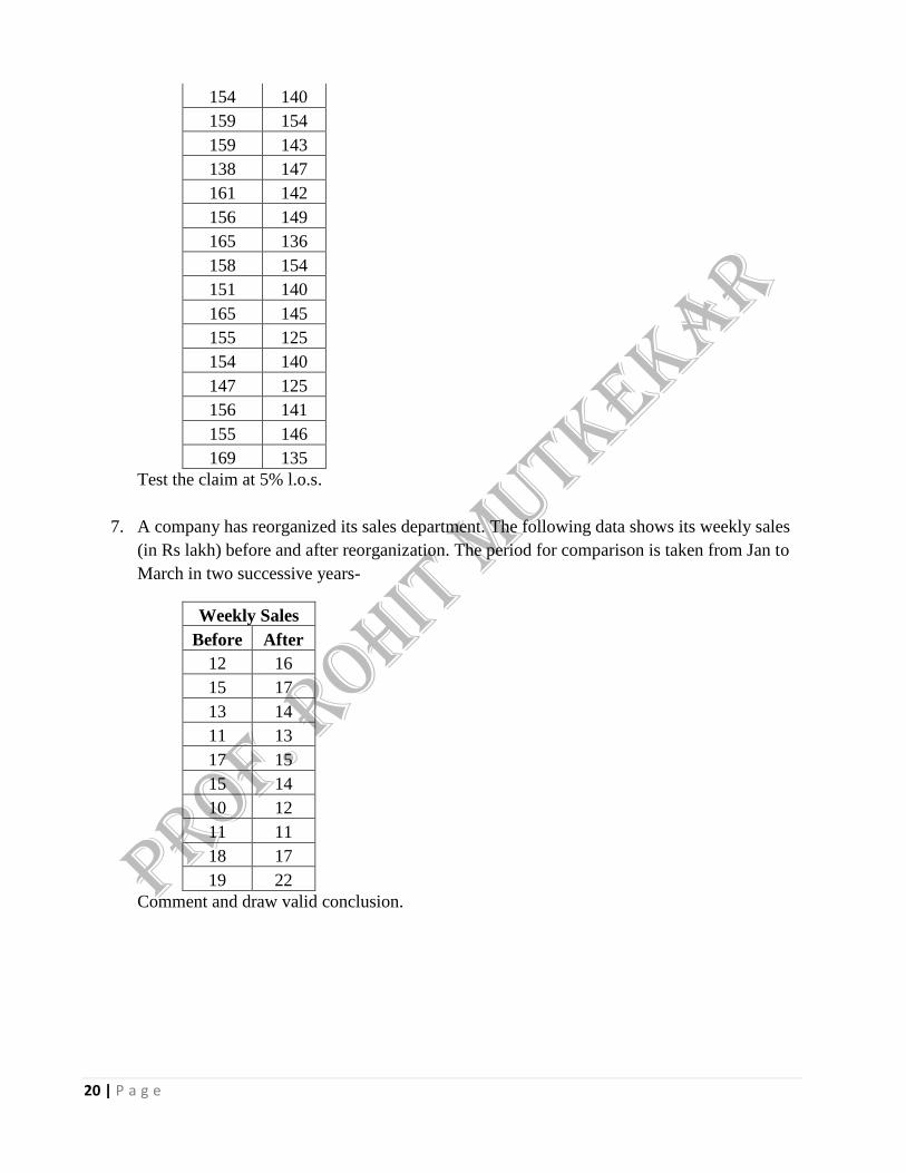
154 140

159 154

159 143

138 147

161 142

156 149

165 136

158 154

151 140

165 145

155 125

154 140

147 125

156 141

155 146

169 135

Test the claim at 5% l.o.s.

7. A company has reorganized its sales department. The following data shows its weekly sales

(in Rs lakh) before and after reorganization. The period for comparison is taken from Jan to

March in two successive years-

Weekly Sales

Before After

12 16

15 17

13 14

11 13

17 15

15 14

10 12

11 11

18 17

19 22

Comment and draw valid conclusion.

21 | P a g e

8. A local pizza restaurant and a local branch of a national chain are located across the street

from a college campus. The local pizza restaurant advertises that it delivers to the dormitories

faster than the national chain. In order to determine whether this advertisement is valid, you

and some of friends have decided to order pizzas from both the outlets at different time. The

delivery times in minutes are as given below-

Local Chain

16.8 22

11.7 15.2

15.6 18.7

16.7 15.6

17.5 20.8

18.1 19.5

14.1 17

21.8 19.5

13.9 16.5

20.8 24


Assignment 3

1. The cinema-goers were 800 people out of a sample of 1000 persons during the period of a

fortnight in a town where no TV programme was aired. Similarly cinema-goers were 700

people out of a sample of 2800 persons during a fortnight where a TV programme was aired.

Do you think that there has been a significant decrease in proportion of cinema-goers due to

the introduction of TV programmes?

2. An insurance agent has claimed that the average age of policy holders who insured through

him is less than the average for all agents which he estimates as 30 years. A random sample

of 100 policy holders who have insured through him gave the following age distribution-

Age in years No of persons insured

16 – 20 12

21 – 25 22

26 – 30 20

31 – 35 30

36 – 40 16


22 | P a g e

3. Two salesmen A and B are working in a certain district. From a sample survey conducted by

the head office, the following results were obtained. State whether there is any significant

difference in the average sales between the two salesmen?

A B

Number of Sales 20 15

Average Sales (in Rs’000) 170 200

Standard Deviation (in Rs’000) 20 25

4. Ten persons were appointed in officer cadre in an office. Their performance was evaluated by

giving a test and the marks were recorded out of 100. They were given two months’ training

and another test was held and the marks were recorded out of 100. The details are as below-

Employees Marks Before Training Marks After Training

A 80 84

B 76 70

C 92 96

D 60 80

E 70 70

F 56 52

G 74 84

H 56 72

I 70 72

J 56 50

Can it be conclude that the employees have benefited by the training?

5. As per the ET-TNS consumer confidence survey, published in Economic Times dt. 10th

November, 2006, the consumer confidence indices for some of the cities changed from

December 2005 to September 2006, as follows. Is the difference significant?

City December 2005 September 2006

Delhi 106 83

Jaipur 117 142

Mumbai 112 126

Ahmedabad 123 108

Kolkota 83 84

Bhubaneshwar 137 144

Bangalore 137 138

Kochi 113 134

23 | P a g e

Chi-Square Test for Independence of Attributes (Theory)


H0: The two attributes are independent


H1: The two attributes are dependent

Here the observed frequencies are given in tabular form called Contingency table.

We need to calculate the expected frequencies using the formula,

𝐸 =𝑅𝑜𝑤 𝑇𝑜𝑡𝑎𝑙 𝑋 𝐶𝑜𝑙𝑢𝑚𝑛 𝑇𝑜𝑡𝑎𝑙

𝐺𝑟𝑎𝑛𝑑 𝑇𝑜𝑡𝑎𝑙


𝜒2𝑜𝑏𝑠

= ∑(𝑂 − 𝐸)2

𝐸 ~ 𝜒2[(𝑟 − 1)x(c − 1)]degree of freedom

Where,

O denotes Observed Frequencies

E denotes Expected Frequencies

r denotes number of rows

c denotes number of columns

Decision Making

We are testing H0 vs H1 at α level of significance, where we can reject H0 if 𝜒2𝑜𝑏𝑠

> 𝜒α2

𝜒α2denotes chi square table value at α level of significance

o Examples on Chi-Square Test for Independence of Attributes

1. The marketing agency gives the following information about the age group of the sample

informants and their liking for a particular model of scooter which a company plans to

introduce:

Age group of the informants

Total Below 20 20-39 40-59

Liked 125 420 60 605

Disliked 75 220 100 395

Total 200 640 160 1000

On the basis of the above data can it be concluded that the model appeal is independent of the

age group of the informants?

24 | P a g e

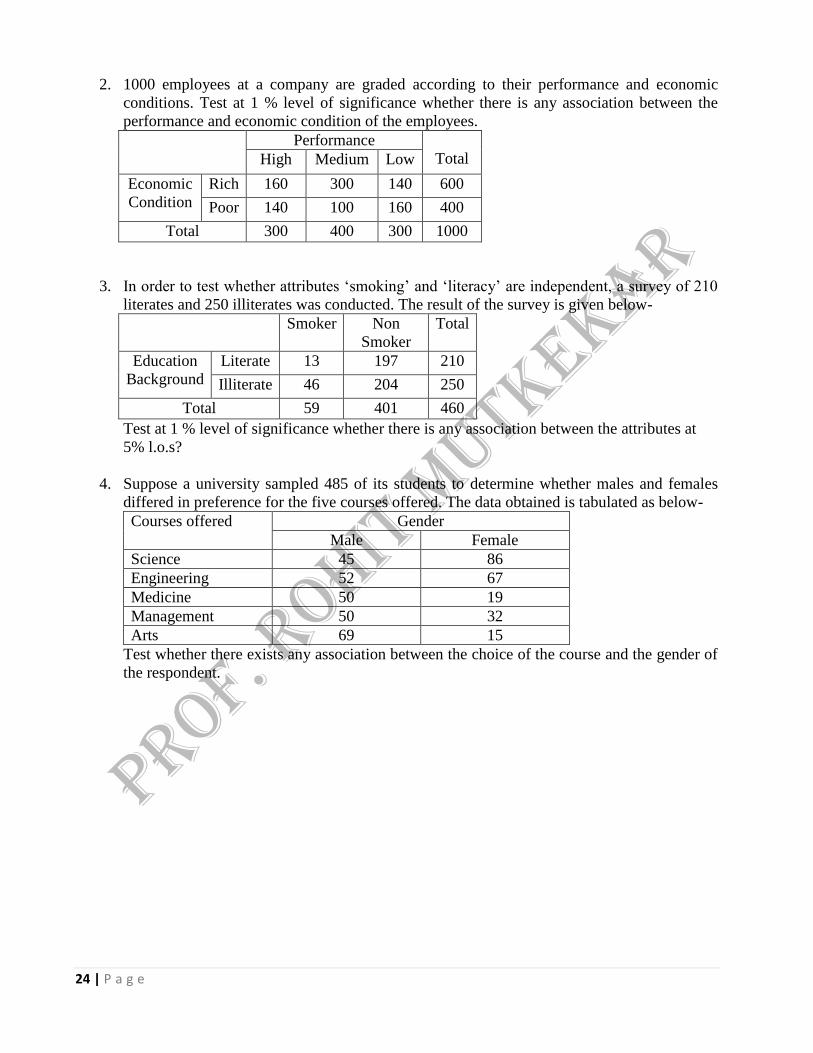
2. 1000 employees at a company are graded according to their performance and economic

conditions. Test at 1 % level of significance whether there is any association between the

performance and economic condition of the employees.

Performance

Total High Medium Low

Economic

Condition

Rich 160 300 140 600

Poor 140 100 160 400

Total 300 400 300 1000

3. In order to test whether attributes ‘smoking’ and ‘literacy’ are independent, a survey of 210

literates and 250 illiterates was conducted. The result of the survey is given below-

Smoker Non

Smoker

Total

Education

Background

Literate 13 197 210

Illiterate 46 204 250

Total 59 401 460

Test at 1 % level of significance whether there is any association between the attributes at

5% l.o.s?

4. Suppose a university sampled 485 of its students to determine whether males and females

differed in preference for the five courses offered. The data obtained is tabulated as below-

Courses offered Gender

Male Female

Science 45 86

Engineering 52 67

Medicine 50 19

Management 50 32

Arts 69 15

Test whether there exists any association between the choice of the course and the gender of

the respondent.

25 | P a g e

Chi-Square Test for Goodness of Fit


H0: The theoretical and observed frequency distribution is a good fit.


H1: The theoretical and observed frequency distribution is not a good fit.


𝜒2𝑜𝑏𝑠

= ∑(𝑂 − 𝐸)2

𝐸 ~ 𝜒2(n − k − 1)degree of freedom

Where,

O denotes Observed Frequencies

E denotes Expected Frequencies

k denotes Additional Constraints

Decision Making

We are testing H0 Vs H1 at α level of significance, where we can reject H0 if 𝜒2𝑜𝑏𝑠

> 𝜒α2

𝜒α2denotes chi-square table value at α level of significance

(Note: If the expected frequencies are found to be less than 5 then it should be pooled with either

the preceding or succeeding frequency term)

o Examples on Chi-Square Test for Independence of Attributes

1. A survey of 64 families with 3 children each is conducted and the number of male children

in each family is noted. The results are tabulated as follows-

No of Male Children 0 1 2 3 Total

No of Families 6 19 29 10 64

Test whether male and female children are equi-probable?

2. The following data relates to the number of mistakes on each page of a book containing 180

pages.

No of Mistakes / page 0 1 2 3 4 ≥5 Total

No of Pages 130 32 15 2 1 0 180

Test whether Poisson distribution is a good fit to the observed distribution.

3. A sample analysis of examination results of 200 MBAs was made. It was found that 46

students had failed, 68 students secured pass class, 62 secured second class and the remaining

secured first class. Are these figures commensurate with the general examination result that is

in the ratio of 2:3:3:2 for various categories respectively? Test at 1% l.o.s.

4. The divisional manager of a retail chain believes that average number of customers entering

each of the five stores in his division weekly is the same. In a given week, the manager reports

the following number of customers in the stores as: 3000, 2960, 3100, 2780, 3160. Test the

divisional manager’s belief at 5% l.o.s.

26 | P a g e

Assignment 4

1. A trainee risk manager for an investment bank has been told that the level of risk is related to

the industry type. For the sample data presented in the contingency table analyze whether

perceived risk is dependent upon the type of industry identified?

Industry Class

Manufacturing Retail Financial

Level of

Risk

Low 81 38 16

Moderate 46 42 33

High 22 26 29

2. An employment agency has recently implemented a new training programme to develop the

interview skills of potential job applicants. Based upon the collected data can we say

confidently that the data can be modelled using binomial distribution? (Test at 1% l.o.s).

No of Interview Successes 0 1 2 3

Frequency 78 143 43 13

3. A motorway safety officer believes that the number of accidents per week occurring on a

stretch of motorway can be modelled using Poisson distribution. A sample data collect for the

study is given below-

No of accidents/week 0 1 2 3 4 5 6 ≥7

Frequency 10 12 12 9 5 3 1 0

Test whether Poisson distribution is a good fit to the observed distribution.

4. A university has recently set up a satellite department within a local college of higher

education. The university claims that 35%, 26%, 25% and 14% of the undergraduate students

are in department A, B, C and D respectively. A random sample of 320 students finds the

following number of students in department A-D: 132, 89, 64 and 35 respectively. Test the

claim at 1% l.o.s.

27 | P a g e

Analysis of Variance (ANOVA)

Introduction

One Way Analysis of Variance (One Way ANOVA) – Theory

Here the null hypothesis is given by

H0: There is no significant difference between the population means

And the corresponding alternative hypothesis is given by

H1: There is a significant difference between atleast one pair of population means

Here the calculation is done using ANOVA table called One Way ANOVA Table

Sources of

Variation

Sum of

Squares

(SS)

Degree of

Freedom

Mean Sum of

Squares

(MSS)

F-Ratio

Between the

Sample

SSB k-1 MSB=SSB/k-1 MSB/MSE

Within the

Sample

SSE n-k MSE=SSE/n-k

Total Variation SST n-1

Now the test statistics is given by-

𝐹𝑜𝑏𝑠 =𝑀𝑆𝐵

𝑀𝑆𝐸 ~ 𝐹(𝑘 − 1, 𝑛 − 𝑘)𝑑𝑒𝑔𝑟𝑒𝑒 𝑜𝑓 𝑓𝑟𝑒𝑒𝑑𝑜𝑚

Here,

n denotes total number of observations

k denotes number of entities under study

Decision Making

We are testing H0 Vs H1 at α level of significance, where we can reject H0 if 𝐹𝑜𝑏𝑠 > 𝐹α

𝐹α denotes F table value at α level of significance

o Examples on One Way ANOVA

1. To assess the significance of possible variation in performance of a company (which has

four plants in different cities) was conducted and the results are given below.

Plant A Plant B Plant C Plant D

08 12 18 13

10 11 12 09

12 09 16 12

08 14 06 16

07 04 08 15

Carry out analysis of variance and interpret the result.

28 | P a g e

2. The following table gives the yields on 15 sample plots under three varieties of seeds namely

A, B and C.

A: 20, 21, 23, 16, 20

B: 18, 20, 17, 15, 25

C: 25, 28, 22, 28, 32

Find out if the average yields of the land with different varieties of seed show significant

differences.

Two Way Analysis of Variance (Two Way ANOVA) without Replication –

Theory

Here the null hypothesis are given by

H0R: There is no significant difference between the factors along the rows

H0C: There is no significant difference between the factors along the columns

And the corresponding alternative hypothesis is given by

H1R: There is a significant difference between the factors along the rows

H1C: There is a significant difference between the factors along the columns

Here the calculation is done using ANOVA table called Two Way ANOVA Table

Sources of

Variation

Sum of

Squares

(SS)

Degree of

Freedom

Mean Sum of

Squares

(MSS)

F-Ratio

Between the

Rows

SSR r-1 MSR=SSR/r-1 MSR/MSE

Between the

Columns

SSC c-1 MSC=SSC/c-1 MSC/MSE

Residual

SSE (r-1)(c-1) MSE=SSE/(r-1)(c-1)

Total Variation SST n-1

Now the test statistics is given by-

𝐹1𝑜𝑏𝑠 =𝑀𝑆𝑅

𝑀𝑆𝐸 ~ 𝐹(𝑟 − 1, (r − 1)(c − 1))𝑑𝑒𝑔𝑟𝑒𝑒 𝑜𝑓 𝑓𝑟𝑒𝑒𝑑𝑜𝑚

𝐹2𝑜𝑏𝑠 =𝑀𝑆𝐶

𝑀𝑆𝐸 ~ 𝐹(𝑐 − 1, (r − 1)(c − 1))𝑑𝑒𝑔𝑟𝑒𝑒 𝑜𝑓 𝑓𝑟𝑒𝑒𝑑𝑜𝑚

Here,

n denotes total number of observations (n=cr)

r denotes number of rows

c denotes number of columns

29 | P a g e

Decision Making

1. We are testing H0R Vs H1R at α level of significance, where we can reject H0 if 𝐹1𝑜𝑏𝑠 >

𝐹1α

𝐹1α denotes F table value at α level of significance for (r-1,(r-1)(c-1))degree of freedom

2. We are testing H0C Vs H1C at α level of significance, where we can reject H0 if 𝐹2𝑜𝑏𝑠 >

𝐹2α

𝐹2α denotes F table value at α level of significance for (c-1,(r-1)(c-1))degree of freedom

o Examples on Two Way Analysis of Variance (Two Way ANOVA) without Replication

3. A company has appointed four salesmen A, B, C and D and observed their sales in three

seasons – summer, winter and monsoon. The figures (in Rs. Lakh) are given in the

following table-

Seasons

Salesmen

A B C D

Summer 36 36 21 35

Winter 28 29 31 32

Monsoon 26 28 29 29

Using 5% l.o.s, perform analysis of variance on the above data and interpret the results.

4. The following data represents the number of units of production per day turned out by

four different workers using five different machines:

Workers

Machine Type

A B C D E

I 4 5 3 7 6

II 5 7 7 4 5

III 7 6 7 8 8

IV 3 5 4 8 2

On the basis of the data given in the table, can it be concluded that-

i. The mean productivity is the same for different machines

ii. The workers don’t differ with regard to productivity.

30 | P a g e

o Examples on Two Way Analysis of Variance (Two Way ANOVA) with Replication

5. The following data refers to the yields of rice on two plots each with combination of the

verity of rice and type of fertilizers

Fertilizer A Fertilizer B Fertilizer C Fertilizer D

Verity 1 6 4 8 6

5 5 6 4

Verity 2 7 6 6 9

6 7 7 8

Verity 3 8 5 10 9

7 5 9 10

Test the above case at 1% l.o.s.

6. Reliable tyre dealer wishes to assess the quality of lives of three different brands of tyres

sold by it. It also wants to assess whether the lives of these tyres is the same for four brands

of cars on which they are been used. Thus, each brand of tyres was tested on each of the

four brands of cars. Further, the dealer wishes to ascertain the equality of lives for each

combination of brands of tyre and car. The mileage obtained are given as follows-

Car A Car B Car C Car D

Tyre 1 32 30 34 36

31 29 33 38

33 28 36 39

31 30 35 40

Tyre 2 38 39 40 41

37 40 41 39

38 41 42 40

39 39 43 42

Tyre 3 32 33 40 45

30 32 42 43

31 30 41 42

33 31 40 46

Test the above case at 5% l.o.s.

31 | P a g e

Assignment 5

1. Three training methods were compared to see if they led to greater productivity after training.

The productivity measures for individuals trained by different methods are as below-

Method 1 36 26 31 20 34 25

Method 2 40 29 38 32 39 34

Method 3 32 18 23 21 33 27

At 1 % l.o.s test whether three training methods lead to different levels of productivity?

2. The following table gives the data on the performance of three different detergents at three

water temperatures. The performance was obtained on the basis ‘whiteness’ readings based

on specially designed equipment for nine loads of washing-

Water Temp.

Detergent

A B C

Cold Water 45 43 55

Warm Water 37 40 56

Hot Water 42 44 46

Analysis the above case using ANOVA at 5% l.o.s.

3. The manager of a bank in Mumbai is responsible for ATM operations in three areas in the

city, viz. Andheri, Vile Parle and Santa Cruz. When he took over the operations, he faced the

problem of cash running out from the ATM machines. To study the problem he collected data

from all the three areas to check whether ATMs in all three areas need equal amount of cash.

He also wanted to know whether ATMs at different locations needed the same amount of cash

or not. So he collected the following data about cash withdrawals(in Rs. Lakhs) during the

last four months which is tabulated as below-

Areas Locations

Station Market Bank

Andheri 40 37 35

39 39 34

41 37 38

39 36 32

Santa Cruz 38 36 34

42 37 35

40 34 33

39 35 34

Vile Parle 38 39 35

39 34 35

39 37 34

41 36 33

Analyze the above case at 1% l.o.s.

Managerial Statistics

Documents

Transcript of Managerial Statistics