MANAGERIAL ECONOMICSINTRODUCTION, BASIC PRINCIPLES

February 17 – March 10, 2014Session 1 - 4

a hypothetical case …

• What if Walmart came to central Europe?

• Get some basic facts about:

– the company– The environment – PESTLE, industry, market, competition

…– Go through the notes up ahead and try to tackle the

hypothetical question

Running a company? Or about to get started? Questions & worries exceed answers and security

• Running a company? Or about to get started? • More questions & worries than answers and security

– How does the economic environment look? What will it be like next and following years? Why?

• What about major econ indicators? -> past, present, future• What about the industry we are in?• What about the market and market segment(s) we are in?

Demand?• What about our decision-making capacity? Resources? Time?

Getting started?

Dealing w/issues from the 1st day of ops & even long before

– A great idea for a product?• because of nonexistence of a competitive product and reasonable

market for it? OR• Because of a huge market although product is NOT unique?

– let’s invest time to look at it …• From a strategic standpoint -> then analyze each factor

– Worth the time and making $ commitments? -> make $ & other types of investments?

• What to invest in? Why? Opportunity cost = vacation in Tahiti?• Where to get $? -> limited resources -> How to appraise the business?• What about Human Capital? Physical assets? Working capital?

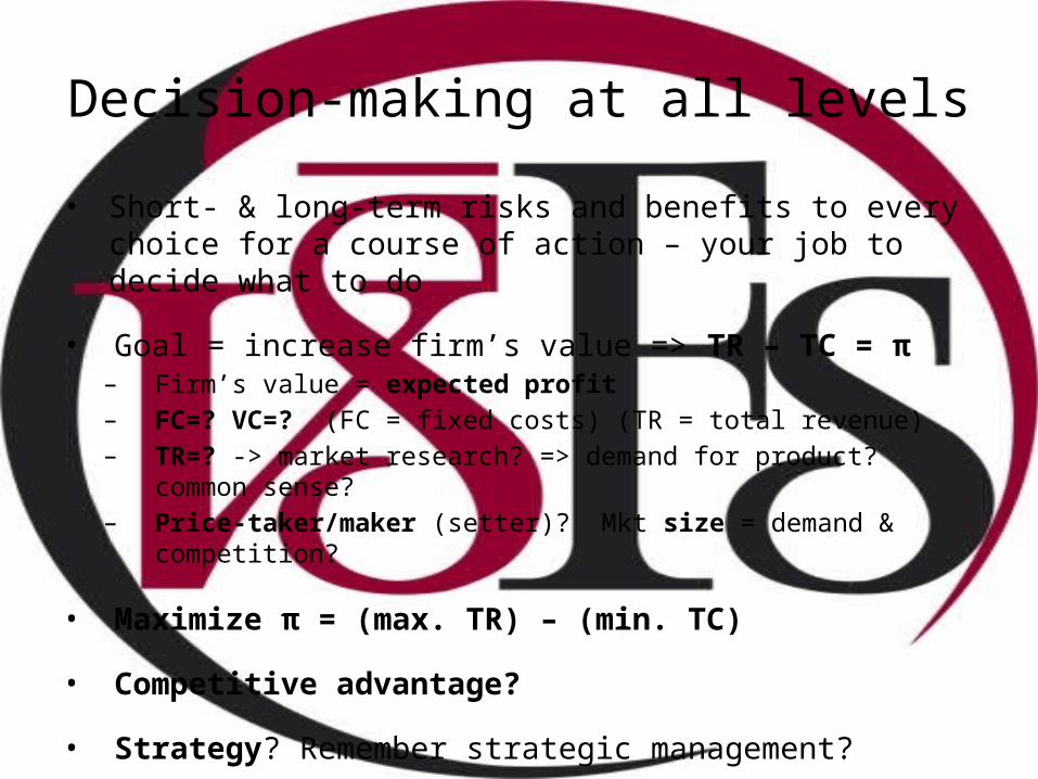
Decision-making at all levels

• Short- & long-term risks and benefits to every choice for a course of action – your job to decide what to do

• Goal = increase firm’s value => TR – TC = π– Firm’s value = expected profit– FC=? VC=? (FC = fixed costs) (TR = total revenue)– TR=? -> market research? => demand for product? common sense?– Price-taker/maker (setter)? Mkt size = demand & competition?

• Maximize π = (max. TR) – (min. TC)

• Competitive advantage?

• Strategy? Remember strategic management?

Strategic Management ModelExisting Existing business model

Mission, vision, goals, objectives, corp. values

SWOT => Strategic

choice

External analysis ->

opportunities, threats

Internal analysis -> strengths,

weaknessesFunctional-level strategies

Business-level strategies

Corporate-level strategies

Strategy implementation

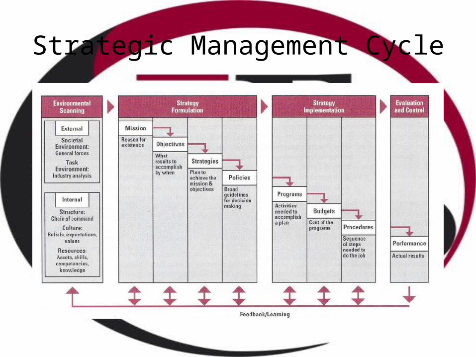
Strategic Management Cycle

Strategic management – mgmt for distant horizons = TOP MANAGEMENT

• Series of destinations which are coming closer with time for everyone– Where was the company yesterday? (if applicable)– Where is the company now ($, ext. environment, market)? What

conditions is it in (internally)?– Where will the company be tomorrow? vs. Where can the company

be tomorrow? vs. Where is the company likely to be tomorrow – if we do a, b, c, or nothing at all?

• Nothing happens by itself =>=> What are the business objectives? -> WHERE TO?=> What are the best ways to achieve these objectives? ->

HOW, WHEN?=> What resources are necessary to execute the plan? ->

w/WHAT & WHOM

From top management down - decisions

• CEO, COO, CFO, CTO – make strategic decisions to optimize => choose between the BAD and WORSE but based on what?

• … on the outcome of analysis of stats data from middle-level management – accounting, $ dept, marketing, HR …

• External & internal environment modify the direction and

pace every day

Common managerial mistakes

• Never increase output just to reduce avg costs

• Grabbing a greater mkt share often times reduces π

• Do NOT maximize π margin -> it does NOT maximize total π

• Maximizing TR reduces π

• Minimizing HR costs => lowers productivity

What assets do we have available?Corporate capital structure

• How do we finance the entire set of:- current operations &- continuity = growth

– Short-term & long-term debt• Issuing bonds• Long-term payables

– Common & preferred equity• Common stock – primary owners (shares) who benefit most• Preferred stock – fixed dividends + NO voting rights like common

shareholders• Retained earnings - $ to be reinvested or pay off debt (surplus

earned)

What assets do we have available?Corporate capital structure

• How much cash-flow should we generate? Why?

• Current assets – used up (utilized) w/in 1 year period– Cash, acc receivables, inventory

• Fixed assets – source of benefits beyond 1-year horizon– Real property (building, real-estate), equipment

Corporate capital structure• Balance sheet (p.237, Exhibit 5-19)

– Liquidity – are we able to meet short-term $ obligations?– Solvency = liquidity with time-dependent factors –> long-term

• Title: International Financial Statement Analysis• Author: Robinson, Thomas

• Sample problem (p. 230, 231)– A & B .. current assets but:

• A … over 50% of assets = cash; B … 6% of assets = cash• A … no current lia’s; B … $2.5 mil of current lia’s !! (cash-flow

fluctuations = death unless B manages to collect receivables or issues more bonds or brings in investors)

• Title: International Financial Statement Analysis• Author: Robinson, Thomas

• Leverage = Little capital = big risk• Debt-to-equity ratio … financing by debt = risk of default• That is – using leverage to invest risky if the investment moves against you => loss is

greater than had the investment been made with equity

Annual reports

• Czech Airlines - annual report 2010 (p.94 - 95)• http://www.csa.cz/en/portal/quicklinks/news/vyrocnizpravy.htm

• Zappos - annual report 2009• http://www.slideshare.net/Devcorporate/zappos-financials-1781754

• BMW - annual report 2012• http://www.bmwgroup.com/e/0_0_www_bmwgroup_com/investor_relations/finanzberichte/ueberblick.shtml

• Your own start-up?• How do you set up your asset, lia, equity structure and why?

Revenues and costs overview

1. From the accounting perspective2. From the “production” perspective

• Maximize π = (max. TR) – (min. TC)

• How do we “know” how much $ we will be making and spending?– Market data - qualitative, quantitative …– Where does it come from?– Available for our product?– Time vs. $ to be invested to get such data– Reliability issues– Price-taker/maker (setter)? - mkt size = demand & competition?

Revenues and costs overviewRevenue Management & Planning

• Some businesses (industries) start off with loss, then swing into 0+ profits, then back to loss and then start making profit

– seasonality factors (ski-resorts, restaurants, hotels, airlines)

• Floating vs. fixed prices– analyzing micro-level consumer behavior and optimizing product

availability and prices => max. profit– dynamic revenue management planning => avg Ps, avg Qs and avg TC– airlines, hotels – choosing the right time to customize the product for

the customer (of our choice)

• Do all industries face seasonalities?

Revenues and costs overview

• Revenue recognition– $ before sale of good/service – unearned revenue– $ at the time of good/service delivery– Good/service before $ - receivables– Examples …

• Expense recognition– Matching principle

• expenses recognized when revenues are recognized

– Systematic allocation of costs –> in the absence of cause & effect• Periods in which benefits are provided -> costs = expenses (accounting)

– Immediate recognition• Costs recognized as expenses because they have no future benefit OR were

recorded as asset and benefits came to end OR neither matching no systematic allocation principles are not uselful

Accounting ratios

• Return on sales = Net profit margin– Net income / revenue– If costs have gone up faster than sales -> lower profit margin

• Operating profit margin– Operating profit / net sales– Profit margin before interest and taxes– Dynamic figures -> comparison needed

• Int’l Financial Statement Analysis – p. 180

Revenues and costs overview

• Plan for & minimize TC = FC + VC– Costing – ABC – activity-based costing– Maximize time and HR efficiencies -> productivity– MRP (material requirement planning) – current expenses

• Costs in short-run– Production function, VC, FC, diminishing marginal product, AC curves,

MC curves, TC, AVC, AP, MP, estimates …

• Costs in long-run– Production isoquants, isocost curves, optimum combination of inputs,

cost optimization (impossible in short-run), long-run vs. short-run …– Chapters 8 – 10 (pp. 284 – 386) – Managerial Economics foundations of business analysis and

strategy, tenth edition – Christopher R. Thomas, S. Charles, Maurice

Bakery – $ analysis

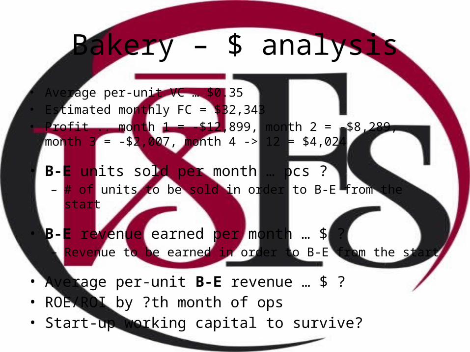
Bakery – $ analysis• Average per-unit VC … $0.35• Estimated monthly FC = $32,343• Profit .. month 1 = -$12,899, month 2 = -$8,289, month 3 = -$2,007,

month 4 -> 12 = $4,024

• B-E units sold per month … pcs ?– # of units to be sold in order to B-E from the start

• B-E revenue earned per month … $ ?– Revenue to be earned in order to B-E from the start

• Average per-unit B-E revenue … $ ?• ROE/ROI by ?th month of ops• Start-up working capital to survive?

Bakery – $ analysis

Bakery – sales & revenue plan

Answers

• B-E units sold per month … 17,255 pcs

• B-E revenue earned per month … $ 38,336

• Average per-unit B-E revenue … $ 2.22

• ROE/ROI by 9th month of ops

• Start-up working capital to survive = $ 23,195

Cost planning, control, analysis – reverse marketing?

• Start-up project/business – set your goals– Budget -> milestones -> operational level breakdown -> back-check ->

evaluation– Project manager OR CEO or executive level -> project manager ->

departments -> reporting to 1 level up at each level -> performance evaluation

• Established operations – objectives defined– Current balance of actual vs. planned expenses => adjust current

budget -> adjust $ for & timing of milestones -> re-adjust op level costs -> evaluation of cost-management performance

– Performance cycle complete -> report to 1 level up at each level -> performance evaluation

Cost planning, control, analysis – closer look

• Budgeting first– total $ available at beginning + new $ coming from external sources– then cost breakdown by milestones/time periods/activities– applying prices to the purchase/hire of inputs within a time frame:

• HR (aka Human Capital)• “raw” material – semi-finished products (tangible items vs. intangible

services)• Inflation, IR• Degree of cost assignment precision – how accurately are costs assigned

to items/activities

• Cost control– Degree of freedom and competency of decision-making at level– Instantaneous checks of actual against planned costs

Cost planning, control, analysis – closer look

• BuffersA. additional time needed for building a back-end mechanism of a

website:1. Individual ops took longer and/or2. Higher expenses incurred by supplier and/or3. Unexpected (unaccounted for) problems/issues occurred

B. Inflation, IR, loss of HR, dynamic developments on the market …

C. HR and legal aspects• Capacity to make decisions and take action• i.e. education (needed and/or required by law), experience

• Use precedent where possible

Cost planning, control, analysis – closer look

What happens if costs exceed $ available?

• Re-allocation / re-distribution of $:– within departments, items– at milestones

• Re-definition of objectives at each level

• More $ obtained– Depending on projected revenues & profits -> ROE, ROI …

Production and costs in the short-runIntro

• Long-run … Q = f (L, K, Ī)– L … variable labor– K … variable capital– Ī … pre-determined (fixed) input … $ investment made for months and years

ahead -> used for acquiring variable K and L over a period in future

• Short-run … Q = f (L, K¯ ) -> Q = f (L)– Capital is purchased for a period ahead -> output varies with varying input =

labor only

• Sunk costs– $ paid for an input and never recovered once the input is no longer needed

• Avoidable costs– $ for inputs we can recover or avoid paying if qty produced = 0

Production in the short-runIntro

• TP = Q, AP = Q/L• MP = ∆Q/∆L = dQ/dL

At Q = 3• dMP/dL = 0 … MP = max• TP starts growing at decreasing rate

At Q = 4• MP = AP• MP must be > AP for AP to grow• E.g. avg grade = 85 -> if you score

80 next time => avg grade drops

Law of diminishing MP• # of PC’s < # of PC employees + space

Production in the short-run Changes in fixed inputs

Buy 2 more PC’s & cars & office => TP (aka Y or Q) grows at any given point – i.e. with the same 5 employees -> # of cruises sold or # of lessons provided or widgets sold grows

Same principle as w/MC

Costs in short-run

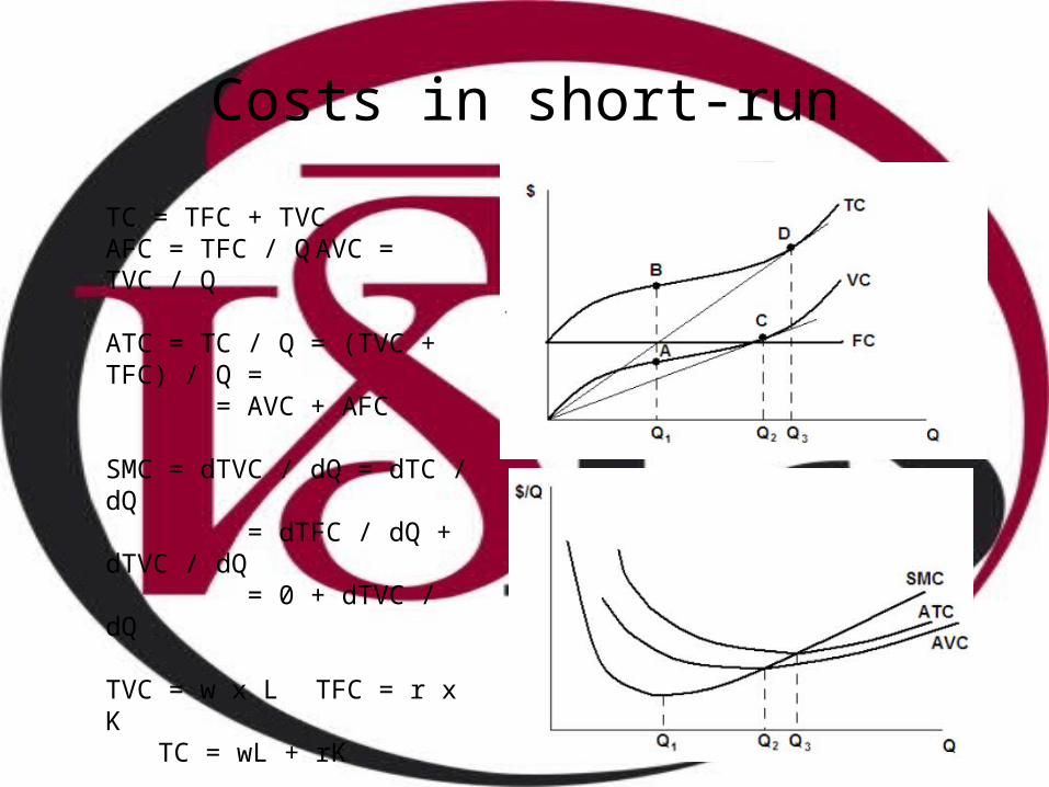
TC = TFC + TVCAFC = TFC / Q AVC = TVC / Q

ATC = TC / Q = (TVC + TFC) / Q = = AVC + AFC

SMC = dTVC / dQ = dTC / dQ = dTFC / dQ + dTVC / dQ = 0 + dTVC / dQ

TVC = w x L TFC = r x KTC = wL + rK

AVC = (wL) / Q = (w x L) / (AP x L) = w / AP

SMC = d(wL) / dQ = w (dL / dQ) = w / MP … w is a constant

Sample problems

PROBLEM 1:Which of the following costs in the airline industry are FC, VC and quasi FC?a. Cost of in-flight good and beveragesb. Jet fuel expendituresc. Pilots’ wagesd. Monthly lease payments for aircraft (48-month term)e. Monthly fee for passenger check-in at its destinations

PROBLEM 2:Q = K²L²K is fixed in s-r at 2 units; cost of K is $3/unitL is a VC; its cost is $4/hourTC=?, production function = ?, L in terms of Q = ?, TFC = ?, TVC = ?, SMC = ?,ATC = ?, AVC = ?, AP = ?, MP = ?

Production and costs in the long-runIntro

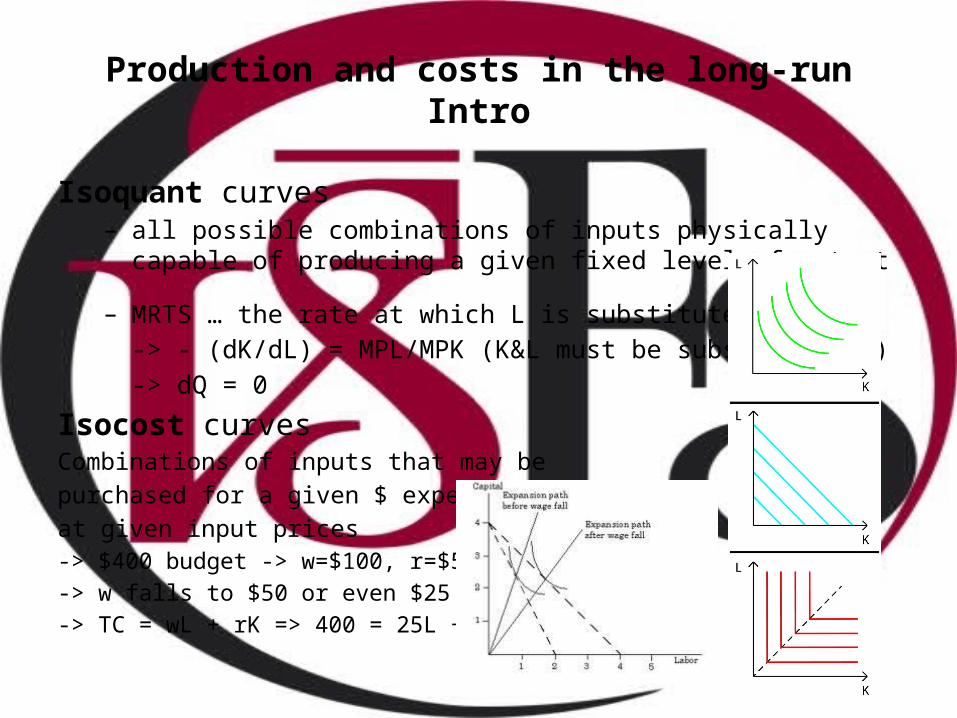
Isoquant curves– all possible combinations of inputs physically capable of producing a

given fixed level of output

– MRTS … the rate at which L is substituted for K-> - (dK/dL) = MPL/MPK (K&L must be substitutable)

-> dQ = 0

Isocost curvesCombinations of inputs that may be purchased for a given $ expenditureat given input prices-> $400 budget -> w=$100, r=$50-> w falls to $50 or even $25-> TC = wL + rK => 400 = 25L + 50K

Production and costs in the long-runOptimal combination of inputs

Slope of isoquant = slope of isocost at optimum

Production and costs in the long-runOptimal combination of inputs

• Searching for:1. Cost minimization

a) Input combination that minimizes TC for a given production levelIf w = $40 and r = $60:

• at S … TC = 60L + 100K = (60x40) + (100x60) = $ 8,400• At Q … TC = (90x40) + (60x60) = $ 7,200 -> MRTS = w/r

b) MP approach to TC minimization -> comparison of MU (benefit) / dollar spent on each activity

- i.e. MU1 / P1 = MU2 / P2 ? -> which activity gives higher marginal benefit

- i.e. at optimal level -> MU1 / P1 = MU2 / P2 -> MRTS = MPL / MPK = w / r -> MPL / w = MPK / r

-> in numbers? What can we arrive at?

Production and costs in the long-runOptimal combination of inputs

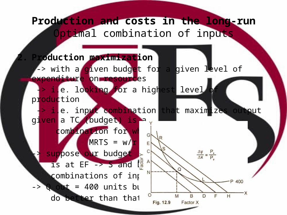
2. Production maximization -> with a given budget for a given level of expenditure on resources -> i.e. looking for a highest level of production -> i.e. input combination that maximizes output given a TC (budget) is a combination for which:

MRTS = w/r … or … MPL/w = MPK / r-> suppose our budget is at EF -> S and L .. 2 of many combinations of inputs X & Y-> Q out = 400 units but we can do better than that

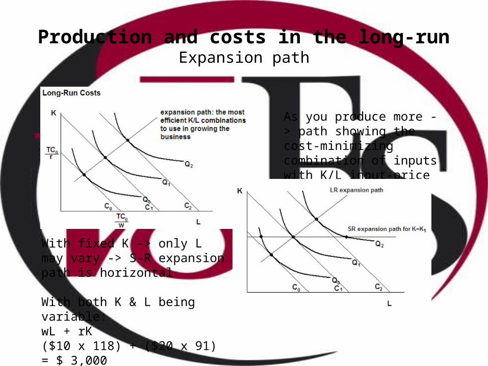
Production and costs in the long-runExpansion path

As you produce more -> path showing the cost-minimizing combination of inputs with K/L input-price ratio held constant

With fixed K -> only L may vary -> S-R expansion path is horizontal

With both K & L being variable:wL + rK($10 x 118) + ($20 x 91) = $ 3,000($10 x 148) + ($20 x 126) = $ 4,000Draw the expansion curve

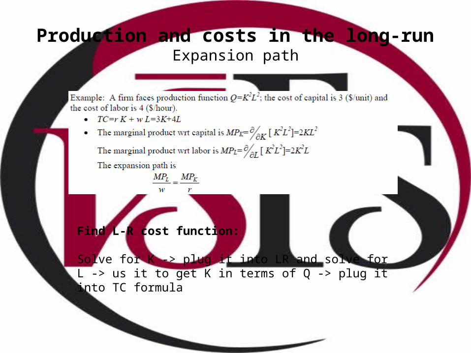
Production and costs in the long-runExpansion path

Find L-R cost function:

Solve for K -> plug it into LR and solve for L -> us it to get K in terms of Q -> plug it into TC formula

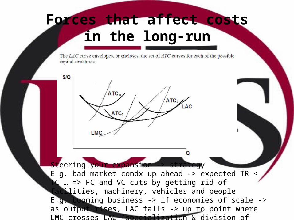
Forces that affect costsin the long-run

Steering your expansion -> strategyE.g. bad market condx up ahead -> expected TR < TC … => FC and VC cuts by getting rid of facilities, machinery, vehicles and peopleE.g. booming business -> if economies of scale -> as output rises, LAC falls -> up to point where LMC crosses LAC (specialization & division of labor => higher productivity => lower unit costs)

Business expansion ?

• Economies of scope– Occurs when the joint cost of producing 2 or more goods/services is

less than the sum of the separate costs of producing the goods/services

• Buying economies of scale– Qty discounts on input prices – large buyers of inputs– i.e. LAC shifts downward at the point of discount

• Learning / experience economies– Cumulative output increases causing workers to become more

productive as they learn by doing => LAC shifts downward