MANAGEMENT OF A SHARED, AUTONOMOUS, ELECTRIC VEHICLE FLEET: 1

IMPLICATIONS OF PRICING SCHEMES 2 3

T. Donna Chen 4

Assistant Professor 5 Department of Civil & Environmental Engineering 6

The University of Virginia 7

tdchen@virginia.edu 8

9 Kara M. Kockelman 10

(Corresponding author) 11 E.P. Schoch Professor of Engineering 12

Department of Civil, Architectural and Environmental Engineering 13

The University of Texas at Austin 14 kkockelm@mail.utexas.edu 15

Phone: 512-471-0210 16

17

ABSTRACT 18 This paper models the market potential of a fleet of shared, autonomous, electric vehicles (SAEVs) 19

by employing a multinomial logit mode choice model in an agent-based framework and different 20 fare settings. The mode share of SAEVs in the simulated mid-sized city (modeled roughly after 21

Austin, Texas) is predicted to lie between 14 and 39%, when competing against privately-owned, 22 manually-driven vehicles and city bus service. This assumes SAEVs are priced between $0.75 and 23 $1.00 per mile, which delivers significant net revenues to the fleet owner-operator, under all 24

modeled scenarios, assuming 80-mile-range electric vehicles and remote/cordless Level II 25 charging infrastructure and up to $25,000 of per-vehicle automation costs. Various dynamic 26

pricing schemes for SAEV fares show that specific fleet metrics can be improved with targeted 27 strategies. For example, pricing strategies that attempt to balance available SAEV supply with 28

anticipated trip demand can decrease average wait times by 19 to 23%. However, tradeoffs also 29 exist within this price-setting: fare structures that favor higher revenue-to-cost ratios (by targeting 30

high-value-of-travel-time [VOTT] travelers) reduce SAEV mode shares, while those that favor 31 larger mode shares (by appealing to a wider VOTT range) produce lower payback. 32 33

KEYWORDS 34 Carsharing, autonomous vehicles, electric vehicles, mode choice, travel costs, taxis 35

INTRODUCTION 36 Technology is quickly changing the landscape of urban transportation. With mobile computing 37

enabling the fast rise of the shared-use economy, carsharing is emerging as an alternative mode 38

that is more flexible than transit but less expensive than traditional (private-vehicle) ownership. 39 Electric vehicle (EV) sales are on the rise with plug-in EVs’ market share growing from 0.14% in 40 2011 to 0.67% in 2014 (Plug in America 2015).Growing plug-in EV adoption should be helpful to 41 most regions in achieving air quality standards for ozone and particulate matter, and ultimately 42 greenhouse gases. Motivated by roadway safety and the growing burden of congested urban 43

driving, automated driving technologies are emerging and private purchases of self-driving 44 vehicles may be possible by 2020 (Bierstadt et al. 2014). 45

There are natural synergies between shared AV (SAV) fleets and EV technology. SAVs resolve 46

the practical limitations of today’s non-autonomous EVs, including traveler range anxiety, access 47 to charging infrastructure/special outlets, and charge-time management. A fleet of shared 48 autonomous electric vehicles (SAEVs) relieves such concerns, by managing range and charging 49

activities based on real-time trip demand and established charging-station locations, as 50 demonstrated in Chen et al. (2016). However, when SAEVs make their debut in cities, these 51 vehicles will not exist in a vacuum. SAEVs will be competing against existing modes (private 52 owned vehicles, transit, and non-motorized modes) for trip share. In this paper, a mode choice 53 model is added to Chen et al.’s (2016) agent-based framework in order to anticipate SAEV market 54

shares in direct competition with other modes. A fleet of 80-mile-range SAEVs is paired with 55 Level II charging infrastructure to deliver relatively fleet operations, and a variety of pricing 56 strategies are employed while examining the shifting mode shares. 57

PRIOR RESEARCH 58

Recent research has examined the operations of self-driving vehicles in a shared setting, primarily 59 focusing on metrics like empty-vehicle miles traveled (VMT), average wait times, and private 60

vehicle replacement rates (Kornhauser et al. [2013], Fagnant and Kockelman [2014], Spieser et al. 61 [2014], ITF [2015], Chen et al. [2016], etc.). Very few have yet simulated AV effects in 62

competition with other modes of travel. 63

Levin and Boyles (2015) recently simulated mode choice of privately-owned AVs (versus transit, 64 private car travel, and walk/bike) with a fixed trip table for a small (downtown) section of Austin, 65

Texas. Their model allows such AVs to strategically re-position themselves to avoid high parking 66 fees (while incurring added fuel costs, but no traveler time costs), and uses dynamic traffic 67

assignment over a 2-hour peak (morning) period. Their special test cases showed transit demand 68 falling as more user classes (segmented by value of travel time [VOTT]) had access to AVs, with 69 61% of low-VOTT travelers decreasing their transit use. They allowed link capacities to rise as a 70

function of the proportion of AVs on each link, so congestion did not worsen as the number of 71

vehicle trips rose sharply (due to empty-vehicle parking repositioning). Childress et al. (2015) used 72 Seattle, Washington’s activity-based travel model (including short-term travel choices and long 73 term work-location and auto-ownership choices) to anticipate AV technology impacts (from higher 74

roadway capacities, lowered VOTTs, reduced parking costs, and increased car-sharing) on 75 regional travel patterns. Their model estimated that higher income households are more likely to 76

choose the AV mode, as expected (since the technology is costly and alternate use of in-vehicle 77 time VOTT reductions for higher-VOTT travelers are likely to be more significant). With SAVs 78

priced at $1.65 per mile (reflecting costs of current ride-sharing taxi services, like Lyft and Uber), 79 drive-alone trips were predicted to fall by one-third and transit shares rose by 140%, as households 80 released traditional vehicles and acquired AVs or turned to SAVs along with other travel options, 81 since they were no longer “tied” to the fixed cost (and round-trip restrictions) of vehicle ownership 82

and storage. 83

The above two simulations are largely limited to private AV ownership (except for one scenario 84 [out of four] in Childress et al. [2015]). Furthermore, their mode choice simulations assumed fixed 85

prices/costs for AV (and SAV) use. Due to the variable nature of SAV availability and user wait 86 times, as well as different costs associated with empty VMT for refueling SAVs and passenger 87 pick-up, SAV pricing may best be “smart-priced” to improve fleet performance metrics. The agent-88 based framework employed in this paper allows for mode choice in the context of each trip (based 89

on a trip’s time-of-day [to allow for “surge pricing” during peak demand periods] and distance, 90

and its traveler’s VOTT) and follows SAEV fleet utilizationthrough a series of simulated travel 91 days to appreciate the effects of various dynamic pricing strategies on mode shares and SAV trip-92 making behaviors. 93

METHODOLOGY 94

The model in this paper builds off of Chen et al.’s (2016) discrete-time agent-based model, 95 which examines the operations of SAEVs and conventionally-fueled SAVs serving roughly 10% 96 of all trips in a 100-mile by 100-mile region. The simulation is gridded to quarter-mile by 97 quarter-mile trip generation and service cells, as shown in Figure 1. Similar to Chen et al. (2016), 98

the trip generation process used here produces each trip based on an average daily rate for each 99 cell (which depends on the local population density, and thus the Euclidean distance to the 100 regional centerpoint in this idealized region), then assigns the destination cell based on trip 101

distance (drawn from the U.S. 2009 National Household Travel Survey’s [NHTS’s] distribution). 102 Average daily trip rates (as shown in Table 1) represent 100% of trips in the simulated region, with rates 103 roughly following the population densities and trip generation rates of Austin, Texas’ travel demand 104 model. Here, a multinomial logit (MNL) mode choice model is added to the agent-based model to 105 allow all trips in the region to choose among private vehicle, transit, and SAEV modes. Trips less 106

than 1 mile in distance (under the NHTS 2009 distribution) are not studied here, since such 107 travelers may often prefer to walk. Since most walking trips in the U.S. are under 1 mile in 108 length, and bike trips are few in the U.S.(Santos et al. 2011), non-motorized modes are not 109

simulated here. 110

111

Figure 1. Regional Zones System 112

Table 1. Total (Motorized) Trip Generation Rates and Travel Speeds by Zone 113

Population Density

(persons/mi2)

Avg Trip Gen. Rate

(trips/cell/day)

SAEV Travel Speed

(mi/hr)

Peak Off-Peak

Downtown 7500-50,000 1287 15 15

Urban 2000-7499 386 24 24

Suburban 500-1999 105 30 33

Exurban <499 7 33 36

114 The amount of money travelers are willing to pay to save travel time and distance varies with each 115 traveler, trip type, day of week, and even driver’s state of mind. To relate each trip to an individual 116 traveler and his/her mode choice in this model, a VOTT is generated for each trip, based on trip 117 purposes and wage rates (per hour). According to the 2009 NHTS, 18.7% of person-trips per 118

household are for work and work-related business trips (Santos et al. 2011). The other 81.3% of 119

trips (for shopping, family/personal errands, school, worship, social, and recreational activities) 120

are combined here, as non-work. After randomly assigning a trip purpose, an income is assigned 121 for the individual traveler based on US Census (2009) data on personal income of individuals 122

residing inside metropolitan areas. SAVs presumably operate more efficiently in densely 123 developed locations than sparsely populated areas (Burns et al. 2013, Fagnant and Kockelman 124

2015), and individual incomes in metro areas tend to be higher than those in rural areas (with 125 personal incomes averaging 33 percent higher, according to US Census [2009]). Hourly wages 126 used in the model here are derived from 2009 Census data on personal income of this living inside 127

metropolitan areas (an average of $48,738 per person per year), and converted to an hourly wage 128 assuming 2000 work hours per year.(US Census 2009).Using USDOT (2011) guidelines, VOTT 129

is assumed to be 50% of hourly wage for personal trips and 100% of hourly wage for business/work 130 trips, yielding Figure 2’s VOTT distributions. 131

132 133

134

0.0

0.1

0.2

0.3

0.4

0.5

0.6

0.7

0.8

0.9

1.0

$0

$3

$6

$8

$11

$14

$17

$20

$22

$25

$28

$31

$34

$36

$39

$42

$45

$48

$50

$53

$56

$59

$62

$64

$67

$70

$73

$76

$78

$81

$84

$87

$90

$92

Mean = $22.95/hr

Median = $16.40/hr

Figure 2a. Work Trips 135

136

137

Figure 2b. Non-Work Trips 138

Figure 2. VOTT Distributions for Work (2a) and Non-Work (2b) Trips 139

In an MNL model, the probability of an individual choosing an alternative is assumed to 140 monotonically increase with that alternative’s systematic utility (Koppelman and Bhat 2006), 141

assuming all other modes’ attributes remain constant, and can be expressed as the following: 142 143

Pr(𝑖) =exp(𝑉𝑖)

exp(𝑉𝑃𝑉)+exp(𝑉𝑇𝑟𝑎𝑛𝑠𝑖𝑡)+exp(𝑉𝑆𝐴𝐸𝑉) (1) 144

145

where 𝑖 denotes the alternative for which the probability is being computed; 𝑉𝑃𝑉, 𝑉𝑇𝑟𝑎𝑛𝑠𝑖𝑡, and 146

𝑉𝑆𝐴𝐸𝑉 denote the systematic utilities of private vehicle, transit, and SAEV, respectively, for a 147 specific origin-destination-traveler-time of day trip. 148

Private Vehicle 149

In this mode choice model, private vehicle utility is modeled as a function of VOTT, operating 150

costs, and parking fees in the destination zone as seen in the equation below: 151 152

𝑉𝑃𝑉 = −𝑉𝑂𝑇𝑇 (𝐷𝑖𝑠𝑡𝑎𝑛𝑐𝑒𝑡𝑟𝑖𝑝

𝑆𝑝𝑒𝑒𝑑𝑃𝑉) − $0.152(𝐷𝑖𝑠𝑡𝑎𝑛𝑐𝑒𝑡𝑟𝑖𝑝) − 𝑃𝑎𝑟𝑘𝑖𝑛𝑔𝐷 (2) 153

154

where 𝑉𝑂𝑇𝑇 is the individual monetary valuation of value of travel time drawn from distributions 155

in Figure 2, 𝐷𝑖𝑠𝑡𝑎𝑛𝑐𝑒𝑡𝑟𝑖𝑝 is the distance of the requested trip, 𝑆𝑝𝑒𝑒𝑑 is equivalent to SAEV 156

average speeds shown in Table 1), $0.152 is the equivalent vehicle operating cost per cell based 157

0.0

0.1

0.2

0.3

0.4

0.5

0.6

0.7

0.8

0.9

1.0$

0$

1

$3

$4

$6

$7

$8

$10

$11

$13

$14

$15

$17

$18

$20

$21

$22

$24

$25

$27

$28

$29

$31

$32

$34

$35

$36

$38

$39

$41

$42

$43

$45

$46

$48

Mean = $11.98/hr Median = $8.50/hr

VOTT ($/hr)

on AAA’s (2014) estimate of $0.608 per mile, and 𝑃𝑎𝑟𝑘𝑖𝑛𝑔𝐷 is the parking fee in the destination 158 zone. In this model, parking cost is assumed to be $0 for all business trips, since 95% of commuters 159 who drive to work park for free at the workplace (Shoup and Breinholt 1997) and other business 160

transportation are often priced in a distorted market with expense accounts. For personal trips, 161 parking for private vehicles is assumed to be $0 for trips that end in suburban or exurban cells, $2 162 for trips that end in urban cells, and $4 for trips that end in downtown cells. 163 164

Transit 165

For simplification, the transit mode modeled here emulates local city bus service, the most 166 common form of transit in US cities. Similar to private vehicles, the utility of the transit mode also 167 depends on transit travel speeds and individual traveler’s VOTT. In addition, access time and fare 168 are considered in the transit utility equation below: 169 170

𝑉𝑡𝑟𝑎𝑛𝑠𝑖𝑡 = −(2) (𝑉𝑂𝑇𝑇

60) (𝐴𝑇𝑂 + 𝐴𝑇𝐷) − 𝑉𝑂𝑇𝑇 (

𝐷𝑖𝑠𝑡𝑎𝑛𝑐𝑒𝑡𝑟𝑖𝑝

𝑆𝑝𝑒𝑒𝑑𝑡𝑟𝑎𝑛𝑠𝑖𝑡) − 𝐹𝑎𝑟𝑒𝑡𝑟𝑎𝑛𝑠𝑖𝑡 (3) 171

172

Where 𝑆𝑝𝑒𝑒𝑑𝑡𝑟𝑎𝑛𝑠𝑖𝑡 is modeled at 25% slower than Table 1’s SAEV speeds during off-peak hours 173

and 20% slower during peak hours due to stops (roughly based on Austin’s travel demand model’s 174

travel time skims), $2 is the assumed one way 𝐹𝑎𝑟𝑒𝑡𝑟𝑎𝑛𝑠𝑖𝑡 based on the $2.04 per unlinked trip 175

fare average from the 2013 National Transit Database Urbanized Data (APTA 2013), and 𝐴𝑇𝑂 and 176

𝐴𝑇𝐷 are the access and wait times in minutes based on the trip’s origin and destination cell 177 following Table 2. 178

Table 2. Transit Access & Wait Time by Zone 179

Zone Transit Access &

Wait Time (min.)

Downtown 3

Urban 9

Suburban 21

Exurban 60

180

Transit access and wait time for exurban cells are penalized (valued at 60 minutes) in the utility 181 function due to the fact that most transit trips to and from exurban areas require transfers (either 182 from private car to transit, or one bus route to another bus route) in the majority of local bus service 183 route designs. Furthermore, access time for transit is modeled at double the VOTT compared to 184 in-vehicle travel time (IVTT). This penalty reflects the general discomfort of time spent walking, 185

bicycling, and waiting outside of vehicles as compared to being inside a vehicle, as recommended 186

in Wardman (2014). Though seated IVTT on transit modes is typically valuated as less onerous 187

than IVTT in a private car (presuming that the traveler can perform more productive or leisure 188 activities while seated on a bus as compared to driving a car), standing IVTT on transit modes is 189 considered more onerous than driving a private vehicle (Wardman 2014). Thus, in this model, 190 transit IVTT is simplified to be valued the same as private vehicle IVTT. 191

SAEV 192

The structure of the SAEV utility valuation (Equation 4) is similar to that of transit, except where 193 transit utility is modeled with a simplified flat price, the SAEV mode incorporates several pricing 194

schemes to examine the impact of pricing on SAEV mode share and fleet operations. The SAEV 195

utility is expressed as: 196 197

𝑉𝑆𝐴𝐸𝑉 = −(2) (𝑉𝑂𝑇𝑇

60) (2.5 + 5𝑛𝑤𝑙𝑖𝑠𝑡) − (0.35)𝑉𝑂𝑇𝑇 (

𝐷𝑖𝑠𝑡𝑎𝑛𝑐𝑒𝑡𝑟𝑖𝑝

𝑆𝑝𝑒𝑒𝑑𝑆𝐴𝐸𝑉) − 𝐹𝑎𝑟𝑒𝑆𝐴𝐸𝑉 (4) 198

199

Where 𝑛𝑤𝑙𝑖𝑠𝑡 is the number of time steps a trip has been on the SAEV waitlist and 𝐹𝑎𝑟𝑒 is the 200 traveler out-of-pocket cost. The first term of this utility function models the onerousness of waiting 201 for an SAEV, valuated at double the IVTT as is done in the transit utility equation. When a trip is 202 generated, the traveler assumes the wait time is 2.5 minutes (half of a time step). If the trip is 203 waitlisted, the traveler re-evaluates mode choice in each of the subsequent time steps the trip 204 remains on the waitlist, and adds 5 minutes to the wait time for each time step the traveler has been 205

on the waitlist. In other words, the longer a trip remains on the waitlist, the more the SAEV utility 206 decreases, and the less likely the traveler will choose SAEV mode. 207

The second term of this utility function models the cost of SAEV IVTT. Unlike transit, a traveler 208 will not have to stand in a SAEV. Thus, a traveler can use the IVTT in a SAEV to work, read, 209 listen to music, or pursue other productive or leisure activities. In the base case, this reduction in 210 travel time cost is modeled at 35% of the IVTT in a non-autonomous private vehicle (where the 211

traveler would be driving), equivalent to the valuation of seated riding time on transit (Concas and 212 Kolpakov 2009). This value is varied in the sensitivity analysis section to examine the impact of 213

IVTT valuation on SAEV mode share. SAEV speeds (shown in Table 1) are assumed to be the 214 same as private vehicle speeds. 215

The last term of the SAEV utility function is the fare. In this model, four pricing strategies are 216

explored: simple distance-based, origin-based, destination-based, and combination pricing. Each 217 pricing scheme is discussed in detail below. 218

Distance-Based Pricing 219

In simple distance-based pricing, the fare is determined proportional to the trip distance as seen in 220

Eq. 5. This pricing scheme is similar to the usage-based (by mileage or time) pricing schemes of 221 current non-autonomous carsharing services. 222 223

𝐹𝑎𝑟𝑒𝑆𝐴𝐸𝑉 = $0.2125 × 𝐷𝑖𝑠𝑡𝑎𝑛𝑐𝑒𝑡𝑟𝑖𝑝 (5) 224

225 Using overhead costs for similarly scaled transit services and assuming operating margins of 10%, 226 Chen et al. (2016) estimate a fleet of SAEVs can be offered at $0.66 to $0.83 per occupied mile of 227 travel, depending on type of fleet vehicles and charging infrastructure. To be conservative, $0.85 228 per mile ($0.2125 per cell) is used as the base fare for simple distance pricing. This per-mile fare 229

is also varied in the sensitivity analysis to examine the effects of higher and lower fares on SAEV 230

market share. 231

Origin-Based Pricing 232

Vehicle relocation is one of the biggest challenges facing operators of non-autonomous carsharing 233 services (see, e.g. Barth and Todd 1999, Correia and Antunes 2012). The origin-based pricing in 234 Equation 6 builds off of Correia and Antunes’ (2012) suggestion that variable pricing policies 235 which encourage trips to balance the demand and availability of vehicles at carsharing stations 236 could contribute to more profitable operations. Here, origin-based pricing attempts to minimize 237

empty vehicles miles traveled for relocation by incentivizing trips originating in a cell that has a 238

surplus of vehicles and penalizing trips originating in a cell that has a deficit of vehicles. 239

240

𝐹𝑎𝑟𝑒𝑆𝐴𝐸𝑉 = ($0.2125 × 𝐷𝑖𝑠𝑡𝑎𝑛𝑐𝑒𝑡𝑟𝑖𝑝)𝑆𝐷𝑀𝑢𝑙𝑡𝑖𝑝𝑙𝑖𝑒𝑟 (6) 241

where 𝑆𝐷𝑀𝑢𝑙𝑡𝑖𝑝𝑙𝑖𝑒𝑟 = 0.5, when (𝑆𝐴𝐸𝑉𝑆𝑢𝑝𝑝𝑙𝑦𝐵,𝑡

𝑆𝐴𝐸𝑉𝑆𝑢𝑝𝑝𝑙𝑦𝑏,𝑡) (

𝑇𝑟𝑖𝑝𝐷𝑒𝑚𝑎𝑛𝑑𝑏,𝑡+1

𝑇𝑟𝑖𝑝𝐷𝑒𝑚𝑎𝑛𝑑𝐵,𝑡+1) < 0.1 242

𝑆𝐷𝑀𝑢𝑙𝑡𝑖𝑝𝑙𝑖𝑒𝑟 = 1, when 10 > (𝑆𝐴𝐸𝑉𝑆𝑢𝑝𝑝𝑙𝑦𝐵,𝑡

𝑆𝐴𝐸𝑉𝑆𝑢𝑝𝑝𝑙𝑦𝑏,𝑡) (

𝑇𝑟𝑖𝑝𝐷𝑒𝑚𝑎𝑛𝑑𝑏,𝑡+1

𝑇𝑟𝑖𝑝𝐷𝑒𝑚𝑎𝑛𝑑𝐵,𝑡+1) > 0.1 243

𝑆𝐷𝑀𝑢𝑙𝑡𝑖𝑝𝑙𝑖𝑒𝑟 = 2, when (𝑆𝐴𝐸𝑉𝑆𝑢𝑝𝑝𝑙𝑦𝐵,𝑡

𝑆𝐴𝐸𝑉𝑆𝑢𝑝𝑝𝑙𝑦𝑏,𝑡) (

𝑇𝑟𝑖𝑝𝐷𝑒𝑚𝑎𝑛𝑑𝑏,𝑡+1

𝑇𝑟𝑖𝑝𝐷𝑒𝑚𝑎𝑛𝑑𝐵,𝑡+1) > 10 244

245

In Eq. 6, 𝑆𝐴𝐸𝑉𝑆𝑢𝑝𝑝𝑙𝑦𝐵,𝑡 is the total number of available SAEVs across all blocks B in the current 246

time step, 𝑆𝐴𝐸𝑉𝑆𝑢𝑝𝑝𝑙𝑦𝑏,𝑡 is the number of vehicles available in the 2-mile by 2-mile block b 247

around the origin cell in the current time step, 𝑇𝑟𝑖𝑝𝐷𝑒𝑚𝑎𝑛𝑑𝑏,𝑡+1 is the number of trips (based on 248

average generation rates shown in Table 1) anticipated to originate from the 2-mile by 2-mile block 249

b surrounding the origin cell in the subsequent time step, and 𝑇𝑟𝑖𝑝𝐷𝑒𝑚𝑎𝑛𝑑𝐵,𝑡+1 is the total trip 250

demand anticipated for the subsequent time step. Essentially, origin-based pricing compares the 251 proportions of trip demand and available vehicle supply in a 2-mile by 2-mile block out of the 252 entire region. Thus, trips that originate in a block with an excess of vehicles (defined by when the 253

product of vehicle supply and trip demand ratios is less than 1) will be cheaper than trips that 254 originate in a block with a deficit of vehicles (defined by when the product of vehicle supply and 255

trip demand ratios is greater than 1). This ratio of ratios is then normalized by the 𝑆𝐷𝑀𝑢𝑙𝑡𝑖𝑝𝑙𝑖𝑒𝑟 256 term, which halves the SAEV fare when supply is at least 10 times greater than demand and 257

doubles the SAEV fare when demand is at least 10 times greater than supply. By incorporating the 258

𝑆𝐷𝑀𝑢𝑙𝑡𝑖𝑝𝑙𝑖𝑒𝑟 term in place of using absolute ratios, extreme pricing scenarios are avoided. It is 259 worth noting that this pricing strategy is rule-based and serves the purpose of illustrating the effect 260

of demand-based pricing on SAEV mode share, but the pricing is not optimized for SAEV fleet 261 performance or profit. 262

Destination-Based Pricing 263

As demonstrated in Chen et al. (2016), up to 5% of a SAEV fleet’s VMT can be attributed to 264 unoccupied miles traveled for charging purposes. The destination-based pricing scheme in 265 Equation 7 attempts to minimize these empty vehicle miles by incentivizing trips that end in a cell 266

close to a charging station site and penalize trips that end in a cell far away from a charging station 267 site. 268 269

𝐹𝑎𝑟𝑒𝑆𝐴𝐸𝑉 = $0.2125(𝐷𝑖𝑠𝑡𝑎𝑛𝑐𝑒𝑡𝑟𝑖𝑝 + 𝐷𝑖𝑠𝑡𝑎𝑛𝑐𝑒𝑐ℎ𝑎𝑟𝑔𝑒) (7) 270

271

In Equation 7, 𝐷𝑖𝑠𝑡𝑎𝑛𝑐𝑒𝑐ℎ𝑎𝑟𝑔𝑒 represents the distance from the destination cell to the closest 272

charging station site. Thus, the destination-based fare prices both occupied miles traveled during 273

the trip and the unoccupied miles traveled to a charging station after a trip is complete. 274

Combination Pricing 275

The last fare structure tested here (Equation 8) is simply a combination of origin- and destination-276 based pricing presented in Equations 6 and 7. 277 278

𝐹𝑎𝑟𝑒𝑆𝐴𝐸𝑉 = $0.2125(𝐷𝑖𝑠𝑡𝑎𝑛𝑐𝑒𝑡𝑟𝑖𝑝 + 𝐷𝑖𝑠𝑡𝑎𝑛𝑐𝑒𝑐ℎ𝑎𝑟𝑔𝑒)𝑆𝐷𝑀𝑢𝑙𝑡𝑖𝑝𝑙𝑖𝑒𝑟 (8) 279

RESULTS 280

In order to understand the impact of introducing a new SAEV mode on existing private vehicle 281

and transit modes, it crucial to examine mode choice in the context of only having the latter two 282 modes. In other words, before introducing SAEVs, what mode would the travelers have chosen 283 for their trips? And what mode will they choose once SAEVs are available? 284

Two-Mode Model 285

Mode choice results from the two-mode model are shown in Table 3. Using the private vehicle 286

and transit utility functions described previously, the model yielded 85.2% private vehicle trips 287 and 14.8% transit trips. For comparison, according to the 2009 American Community Survey, 288 76.4% of US workers who live and work inside the same metropolitan area commute by drive 289

alone mode and 7.8% commute by public transit (McKenzie and Rapino 2011). While trips with 290 low VOTT are served by both private vehicle and transit modes (both with minimum VOTTs of 291 $0), trips valuated at over $21.20 per hour are only served by private vehicles. The long right tail 292

of the VOTT distribution for private vehicle trips (with maximum VOTT at $90.80 per hour) is 293 evident when looking at averages: mean VOTT for a private vehicle trip is 4.5 times the mean 294 VOTT for a transit trip. In a similar manner, short trips are served by both private vehicles and 295

transit, but transit is consistently the preferred mode for longer trips (over 119 miles). 296

In the simplified transit pricing modeled here, longer trips will incur higher operating costs for 297

private vehicles while fare remains flat at $2 for transit, hence the preference for transit mode as 298 trip lengths grow longer. Model results also show that where there are significant parking costs, 299 transit is preferred over private vehicle mode. Hypothetically, trips served by transit would have 300

averaged $1.15 in parking fees per trip had the trips been served by private vehicle. Trips that 301

actually chose private vehicle mode averaged just $0.32 in parking fees per trip. Likewise, when 302 transit access times are significant, private vehicle mode is preferred. Trips that chose transit mode 303 had an average total origin and destination access time of 44 minutes, while trips that chose private 304

vehicle mode would have hypothetically averaged 74 minutes for origin and destination access 305 had transit mode been chosen. 306

Table 3. Attributes of Private-Vehicle and Transit Trips in Two-Mode Model 307

Private-Vehicle

Trips

Transit

Trips

Mode Share 85.19% 14.81%

VOTT

($/hr)

Mean $16.16 $3.56

Median $11.40 $2.75

Std Dev $15.04 $3.29

Max $90.80 $21.20

Min $0.00 $0.00

Trip Distance (mi)

Mean 8.83 17.21

Median 5.00 10.13

Std Dev 10.83 19.47

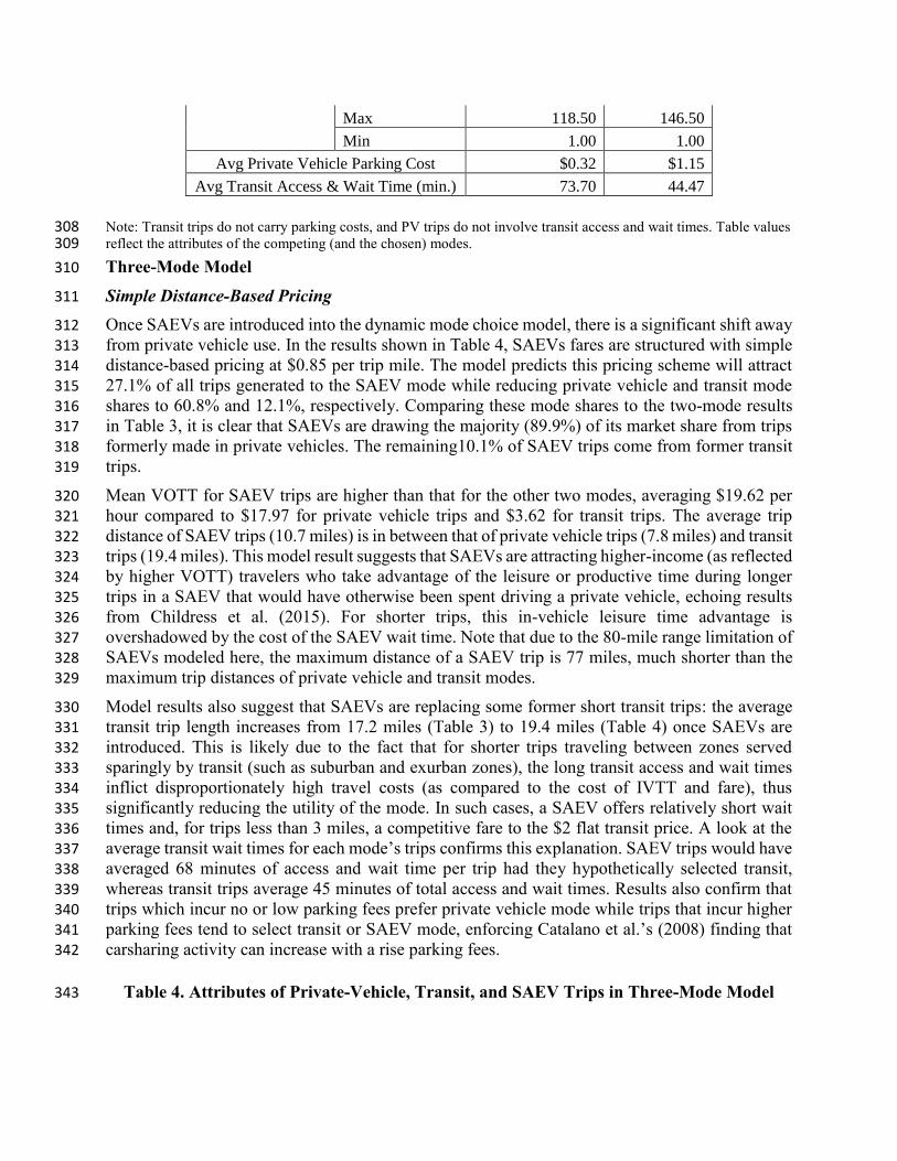
Max 118.50 146.50

Min 1.00 1.00

Avg Private Vehicle Parking Cost $0.32 $1.15

Avg Transit Access & Wait Time (min.) 73.70 44.47

Note: Transit trips do not carry parking costs, and PV trips do not involve transit access and wait times. Table values 308 reflect the attributes of the competing (and the chosen) modes. 309

Three-Mode Model 310

Simple Distance-Based Pricing 311

Once SAEVs are introduced into the dynamic mode choice model, there is a significant shift away 312 from private vehicle use. In the results shown in Table 4, SAEVs fares are structured with simple 313 distance-based pricing at $0.85 per trip mile. The model predicts this pricing scheme will attract 314

27.1% of all trips generated to the SAEV mode while reducing private vehicle and transit mode 315 shares to 60.8% and 12.1%, respectively. Comparing these mode shares to the two-mode results 316

in Table 3, it is clear that SAEVs are drawing the majority (89.9%) of its market share from trips 317 formerly made in private vehicles. The remaining10.1% of SAEV trips come from former transit 318

trips. 319

Mean VOTT for SAEV trips are higher than that for the other two modes, averaging $19.62 per 320 hour compared to $17.97 for private vehicle trips and $3.62 for transit trips. The average trip 321

distance of SAEV trips (10.7 miles) is in between that of private vehicle trips (7.8 miles) and transit 322 trips (19.4 miles). This model result suggests that SAEVs are attracting higher-income (as reflected 323

by higher VOTT) travelers who take advantage of the leisure or productive time during longer 324 trips in a SAEV that would have otherwise been spent driving a private vehicle, echoing results 325 from Childress et al. (2015). For shorter trips, this in-vehicle leisure time advantage is 326

overshadowed by the cost of the SAEV wait time. Note that due to the 80-mile range limitation of 327

SAEVs modeled here, the maximum distance of a SAEV trip is 77 miles, much shorter than the 328 maximum trip distances of private vehicle and transit modes. 329

Model results also suggest that SAEVs are replacing some former short transit trips: the average 330

transit trip length increases from 17.2 miles (Table 3) to 19.4 miles (Table 4) once SAEVs are 331 introduced. This is likely due to the fact that for shorter trips traveling between zones served 332 sparingly by transit (such as suburban and exurban zones), the long transit access and wait times 333

inflict disproportionately high travel costs (as compared to the cost of IVTT and fare), thus 334 significantly reducing the utility of the mode. In such cases, a SAEV offers relatively short wait 335 times and, for trips less than 3 miles, a competitive fare to the $2 flat transit price. A look at the 336 average transit wait times for each mode’s trips confirms this explanation. SAEV trips would have 337 averaged 68 minutes of access and wait time per trip had they hypothetically selected transit, 338

whereas transit trips average 45 minutes of total access and wait times. Results also confirm that 339 trips which incur no or low parking fees prefer private vehicle mode while trips that incur higher 340

parking fees tend to select transit or SAEV mode, enforcing Catalano et al.’s (2008) finding that 341 carsharing activity can increase with a rise parking fees. 342

Table 4. Attributes of Private-Vehicle, Transit, and SAEV Trips in Three-Mode Model 343

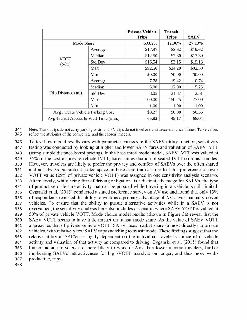
Private Vehicle

Trips

Transit

Trips SAEV

Mode Share 60.82% 12.08% 27.10%

VOTT

($/hr)

Average $17.97 $3.62 $19.62

Median $12.50 $2.80 $13.30

Std Dev $16.54 $3.15 $19.13

Max $92.50 $24.20 $92.50

Min $0.00 $0.00 $0.00

Trip Distance (mi)

Average 7.78 19.42 10.74

Median 5.00 12.00 5.25

Std Dev 8.05 21.37 12.51

Max 100.00 150.25 77.00

Min 1.00 1.00 1.00

Avg Private Vehicle Parking Cost $0.27 $0.88 $0.56

Avg Transit Access & Wait Time (min.) 65.82 45.17 68.04

Note: Transit trips do not carry parking costs, and PV trips do not involve transit access and wait times. Table values 344 reflect the attributes of the competing (and the chosen) models. 345

To test how model results vary with parameter changes to the SAEV utility function, sensitivity 346

testing was conducted by looking at higher and lower SAEV fares and valuation of SAEV IVTT 347 (using simple distance-based pricing). In the base three-mode model, SAEV IVTT was valued at 348 35% of the cost of private vehicle IVTT, based on evaluation of seated IVTT on transit modes. 349

However, travelers are likely to prefer the privacy and comfort of SAEVs over the often shared 350 and not-always guaranteed seated space on buses and trains. To reflect this preference, a lower 351

VOTT value (25% of private vehicle VOTT) was assigned in one sensitivity analysis scenario. 352 Alternatively, while being free of driving obligations is a distinct advantage for SAEVs, the type 353

of productive or leisure activity that can be pursued while traveling in a vehicle is still limited. 354 Cyganski et al. (2015) conducted a stated preference survey on AV use and found that only 13% 355

of respondents reported the ability to work as a primary advantage of AVs over manually-driven 356 vehicles. To ensure that the ability to pursue alternative activities while in a SAEV is not 357

overvalued, the sensitivity analysis here also includes a scenario where SAEV VOTT is valued at 358 50% of private vehicle VOTT. Mode choice model results (shown in Figure 3a) reveal that the 359 SAEV VOTT seems to have little impact on transit mode share. As the value of SAEV VOTT 360 approaches that of private vehicle VOTT, SAEV loses market share (almost directly) to private 361 vehicles, with relatively few SAEV trips switching to transit mode. These findings suggest that the 362

relative utility of SAEVs is highly dependent on the individual traveler’s choice of in-vehicle 363 activity and valuation of that activity as compared to driving. Cyganski et al. (2015) found that 364

higher income travelers are more likely to work in AVs than lower income travelers, further 365 implicating SAEVs’ attractiveness for high-VOTT travelers on longer, and thus more work-366 productive, trips. 367 368

369

Figure 3a. Mode Share Sensitivity to SAEV VOTT Effects 370

371

372

Figure 3b. Mode Share Sensitivity to SAEV Fares 373

57.90%

60.82%

67.66%

11.46%

12.08%

12.84%

30.64%

27.10%

19.51%

0.25

0.35

0.50

Private Vehicle Transit SAEVS

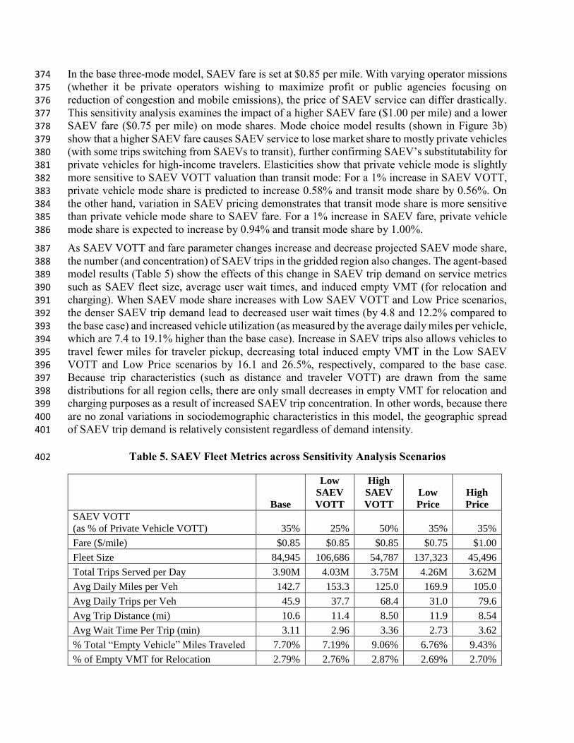
AE

V V

OT

T/P

rivat

e V

ehic

le V

OT

T

71.42%

60.82%

50.31%

14.22%

12.08%

10.64%

14.36%

27.10%

39.05%

$1.00

$0.85

$0.75

Private Vehicle Transit SAEV

SA

EV

Pri

ce

($/m

ile)

In the base three-mode model, SAEV fare is set at $0.85 per mile. With varying operator missions 374

(whether it be private operators wishing to maximize profit or public agencies focusing on 375 reduction of congestion and mobile emissions), the price of SAEV service can differ drastically. 376 This sensitivity analysis examines the impact of a higher SAEV fare ($1.00 per mile) and a lower 377

SAEV fare ($0.75 per mile) on mode shares. Mode choice model results (shown in Figure 3b) 378 show that a higher SAEV fare causes SAEV service to lose market share to mostly private vehicles 379 (with some trips switching from SAEVs to transit), further confirming SAEV’s substitutability for 380 private vehicles for high-income travelers. Elasticities show that private vehicle mode is slightly 381 more sensitive to SAEV VOTT valuation than transit mode: For a 1% increase in SAEV VOTT, 382

private vehicle mode share is predicted to increase 0.58% and transit mode share by 0.56%. On 383 the other hand, variation in SAEV pricing demonstrates that transit mode share is more sensitive 384 than private vehicle mode share to SAEV fare. For a 1% increase in SAEV fare, private vehicle 385 mode share is expected to increase by 0.94% and transit mode share by 1.00%. 386

As SAEV VOTT and fare parameter changes increase and decrease projected SAEV mode share, 387 the number (and concentration) of SAEV trips in the gridded region also changes. The agent-based 388

model results (Table 5) show the effects of this change in SAEV trip demand on service metrics 389 such as SAEV fleet size, average user wait times, and induced empty VMT (for relocation and 390

charging). When SAEV mode share increases with Low SAEV VOTT and Low Price scenarios, 391 the denser SAEV trip demand lead to decreased user wait times (by 4.8 and 12.2% compared to 392 the base case) and increased vehicle utilization (as measured by the average daily miles per vehicle, 393

which are 7.4 to 19.1% higher than the base case). Increase in SAEV trips also allows vehicles to 394 travel fewer miles for traveler pickup, decreasing total induced empty VMT in the Low SAEV 395

VOTT and Low Price scenarios by 16.1 and 26.5%, respectively, compared to the base case. 396 Because trip characteristics (such as distance and traveler VOTT) are drawn from the same 397 distributions for all region cells, there are only small decreases in empty VMT for relocation and 398

charging purposes as a result of increased SAEV trip concentration. In other words, because there 399

are no zonal variations in sociodemographic characteristics in this model, the geographic spread 400 of SAEV trip demand is relatively consistent regardless of demand intensity. 401

Table 5. SAEV Fleet Metrics across Sensitivity Analysis Scenarios 402

Base

Low

SAEV

VOTT

High

SAEV

VOTT

Low

Price

High

Price

SAEV VOTT

(as % of Private Vehicle VOTT) 35% 25% 50% 35% 35%

Fare ($/mile) $0.85 $0.85 $0.85 $0.75 $1.00

Fleet Size 84,945 106,686 54,787 137,323 45,496

Total Trips Served per Day 3.90M 4.03M 3.75M 4.26M 3.62M

Avg Daily Miles per Veh 142.7 153.3 125.0 169.9 105.0

Avg Daily Trips per Veh 45.9 37.7 68.4 31.0 79.6

Avg Trip Distance (mi) 10.6 11.4 8.50 11.9 8.54

Avg Wait Time Per Trip (min) 3.11 2.96 3.36 2.73 3.62

% Total “Empty Vehicle” Miles Traveled 7.70% 7.19% 9.06% 6.76% 9.43%

% of Empty VMT for Relocation 2.79% 2.76% 2.87% 2.69% 2.70%

% of Empty VMT for Charging 1.81% 1.83% 1.77% 1.79% 1.82%

% of Empty VMT for Traveler Pickup 3.10% 2.60% 4.43% 2.28% 4.90%

Max % of Concurrent In-Use Vehicles 38.6% 41.5% 34.7% 48.1% 29.1%

Max % of Concurrent Charging Vehicles 53.5% 54.1% 47.99% 58.0% 40.7%

Operational Cost per Equivalent Occupied

Mile Traveled $0.389 $0.383 $0.400 $0.378 $0.409

Daily Revenue $9.41M $12.8M $5.24M $16.2M $4.29M

Revenue-to-Cost Ratio 2.00 2.04 1.92 1.85 2.19

403

Interestingly, the average trip distance of scenarios with high SAEV trip demand (Low SAEV 404 VOTT and Low Price) are longer than those of scenarios with low SAEV trip demand (High SAEV 405 VOTT and High Price). So while the vehicles in high-demand scenarios are utilized for more miles 406 each day, they actually serve fewer trips per day. However, the households who take these longer 407

trips as SAEV VOTT and fare decrease are different, as reflected by the revenue to cost ratios. 408 Both the Low SAEV VOTT and Low Price scenarios demand a bigger fleet (to serve increased 409

SAEV demand) compared to the base case, but the Low SAEV VOTT scenario registers a bigger 410 profit margin than the base case while the Low Price scenario does the opposite. As discussed 411 previously, travelers who can do productive work while traveling in a SAEV will view their time 412

in a SAEV as less costly, especially as trip distances increase. In the Low SAEV VOTT scenario, 413 more high income travelers’ longer trips are captured by SAEV mode. On the other hand, the Low 414

Price scenario captures longer trips from lower income travelers, as the advantage of SAEVs’ 415 shorter wait times outweigh the fare advantage of transit in trips that travel between suburban and 416 exurban zones. 417

Overall, the largest absolute daily revenue is generated by the Low Price scenario, simply due to 418 the significantly increased trip demand. However, when revenue is compared to costs, the High 419

Price scenario yields the most favorable ratio. 420

Origin, Destination, and Combination Pricing 421

Sensitivity testing results revealed that different assumptions in SAEV VOTT and fare results in a 422 wide range (14-39%) of SAEV mode shares. These different trip demands require different 423

infrastructure investments and location placements to accommodate increasing and decreasing trip 424 densities. They also heavily impact revenue and profit margins, as shown in Table 5. 425

Next, this study analyzes how various pricing strategies can affect fleet operations (with the same 426 vehicle fleet size, charging infrastructure, and trip demand). Table 6’s results employ the charging 427

strategies described in the Mode Choice Methodology section, all assuming SAEV VOTT to be 428 35% of private vehicle VOTT and a base distance pricing of $0.85 per mile. 429 430

Pricing Scheme

Distance-

Based

Origin-

Based

Destination-

Based Combo

Private Vehicle Mode Share 60.8% 63.9% 67.2% 68.6%

Avg Private Vehicle VOTT ($/hr) $17.97 $17.57 $17.01 $17.57

Avg Private Vehicle Trip Distance (mi) 7.78 8.31 7.67 8.16

Transit Mode Share 12.1% 11.7% 12.0% 13.1%

Avg Transit VOTT ($/hr) $3.62 $3.58 $3.31 $3.57

Avg Transit Trip Distance (mi) 19.4 19.1 18.2 18.7

SAEV Mode Share 27.1% 24.4% 20.8% 18.3%

Avg SAEV VOTT ($/hr) $19.62 $18.78 $21.92 $23.17

Avg SAEV Trip Distance (mi) 10.6 10.1 12.6 12.2

Total Trips Served per Day 3.90M 3.85M 3.72M 3.68M

Avg Daily Miles per Veh 142.7 122.6 117.1 101.2

Avg Daily Trips per Veh 45.9 45.3 43.9 43.3

Avg Wait Time Per Trip (min) 3.11 2.51 3.03 2.40

% Total “Empty Vehicle” Miles Traveled 7.70% 8.11% 7.37% 7.83%

% of Empty VMT for Relocation 2.79% 3.72% 3.11% 4.24%

% of Empty VMT for Charging 1.81% 1.98% 1.80% 2.02%

% of Empty VMT for Traveler Pickup 3.10% 2.41% 2.46% 1.57%

Operational Cost per Equivalent

Occupied Mile Traveled $0.389 $0.398 $0.395 $0.405

Daily Revenue $9.41M $8.16M $8.35M $7.27M

Revenue to Cost Ratio 2.00 1.97 2.12 2.08

Table 6: SAEV Fleet Metrics across Distinctive Pricing Strategies 431

Compared to distance-based pricing, the origin-based pricing scheme seems effective in reaching 432

a more balanced vehicle supply and demand. This is reflected by the 22.3% reduction in 433 unoccupied VMT for traveler pickup (compared to distance-based pricing), which then 434 corresponds to a 19.3% reduction in average SAEV wait times. However, this efficiency 435

improvement comes with a 10% reduction in SAEV demand (mode share drops from 27.1% in 436 distance-based pricing to 24.4% in origin-based pricing) and 13.3% decrease in daily revenue. The 437

disproportionate revenue reduction is a result of discounted SAEV trips being more accessible to 438 lower-VOTT households, as witnessed in the 4.3% reduction in average SAEV VOTT between 439

distance- and origin-based pricing. 440

Destination-based pricing, compared to distance-based pricing, exhibits a negligible (less than 1%) 441

reduction in empty VMT for charging purposes. Due to the coverage-maximizing nature of the 442 charging station site generation methodology used here (discussed in detail in Chen et al. [2016]), 443 the distance between the destination cell and the nearest charging station varies little. However, 444 this pricing scheme did have the effect of discouraging shorter trips from choosing SAEV mode, 445

as the charging surcharge of the SAEV fare becomes a larger portion of the overall fare as trip 446 distances decrease. As discussed previously, high-VOTT travelers favor long SAEV trips. Thus, 447 the decrease in short SAEV trips is accompanied by an 11.7% increase in average SAEV VOTT. 448

The combination pricing scheme results shows some characteristics of both the origin- and 449

destination-based pricing schemes: Average SAEV wait times are reduced by 22.8% and average 450 SAEV VOTT increases 18.1%. The performance metrics of the combination pricing scheme seems 451 to have two aspects which appeal to time-sensitive/high-VOTT travelers: minimized wait times 452

and pricing which favors longer-distance trips. This pricing scheme also resulted in the highest 453 transit mode share and lowest SAEV mode share. 454

SUMMARY AND CONCLUSIONS 455

This study explores the impact of pricing strategies on SAEV market share in a discrete-timed 456 agent-based model of a simulated region with private vehicle, transit, and SAEVs serving as the 457

mode choice alternatives. The model specification delivers roughly an 85%/15% split between 458

private vehicles and transit trips before the introduction of SAEVs. When the SAEV mode is 459 offered at $0.85 per mile (and users are assumed to value SAEV IVTT at 35% the cost of private 460 vehicle IVTT), the model estimates that 27% of all person-trips in the region (of at least 1 mile in 461

distance) will select SAEVs (with 90% of these trips previously choosing private vehicle travel, 462 before introduction of SAEVs). 463

Sensitivity analysis suggests that SAEV market share can range from 14% to 39% under plausible 464 variations in SAEV VOTT and fare assumptions. Under all scenarios, SAEVs prove to be 465 substitutable for private vehicle travel, assuming that single-occupant shared vehicle trips offer 466

equal utility as single-occupant private vehicle trips for all trip types While private vehicle mode 467 share is most sensitive to persons’ VOTT during SAEV travel, transit mode share is most sensitive 468 to SAEV fare assumptions. These results suggest that once EV and AV technologies gain market 469 maturity and become less costly, low-VOTT trip makers will start to choose SAEVs over transit, 470

particularly in areas with poor transit service (as reflected by longer transit-access and wait times), 471 echoing findings from Levin and Boyles’ (2015) center-city, peak-period simulation. Model results 472

also suggest that SAEVs will attract longer trips away from private vehicles, particularly among 473 high-VOTT travelers who find SAEV travel much less burdensome than driving. Vehicle features 474

that encourage and enhance work productivity (such as reliable WiFi, ergonomic work surfaces 475 and seating, and reduced road noise) will likely attract longer trips from high-VOTT travelers 476 willing to pay higher fares (Mokhtarian et al. 2013). Like airlines, public SAEV operators may 477

find the best balance of profitability and service completeness by offering a refined, work-478 enhancing vehicle environment at higher fares to serve high-VOTT travelers (similar to the first- 479

and business-class airplane cabins) and a discounted, sufficiently basic service to serve low-VOTT 480 travelers (similar to economy-class airplane cabins). 481

Model outputs from various SAEV pricing schemes show that specific fleet metrics can be 482

improved via targeted strategies. For example, fares that seek to balance available SAEV supply 483

with anticipated trip demand (over space and time) can decrease average wait times by 19 to 23%, 484 demonstrating the effectiveness of congestion pricing in a vehicle-balancing framework. However, 485 trade-offs are evident in these pricing schemes: fare structures that favor higher revenue-to-cost 486

ratios (by targeting higher-VOTT travelers) inevitably reduce SAEV mode shares, while those that 487 favor greater market share (by appealing to a wider range of travelers and VOTTs) inevitably 488

produce lower revenue-to-cost ratios. These pricing outputs emphasize the role of the SAEV 489 operators’ goals when selecting a fare structure. For private SAEV operators, whose goal typically 490

is to maximize profits, a combination pricing scheme that minimizes user wait times while 491 discouraging shorter trips (which tend to incur a higher level of empty VMT-to-occupied VMT) 492 are most suitable. For a public SAEV operator, whose goal presumably is to maximize equitable 493 access to SAEVs while still reducing wait times, a supply-and-demand (origin-based) pricing 494 scheme may be most suitable. 495

496 The model outputs also reinforce the importance of efficient parking prices, since SAEVs will be 497

more competitive against private vehicles in areas which prices parking marginally according to 498 usage rather than subsidies through development policies (e.g. requiring developers to provide 499 specific numbers of parking spaces per retail square footage) or employer-provided 500 benefits.Under-priced and inefficiently-priced parking spaces in most U.S. and non-U.S. cities 501 play a direct role in increasing traffic congestion, housing inaffordability, sprawl, and mobile-502 source emissions (Litman 2011). Inefficient parking prices also cause undervaluation of one of 503

SAEVs’ key benefits: reduced parking demand (and out-of-pocket parking costs), decreasing their 504

competitive advantage relative to private vehicles. 505

The pricing strategies and sensitivity analysis explored here offer insights on the many factors that 506 influence SAEV mode shares and fleet performance. However, this agent-base model and 507

application is limited in various ways. For example, more than three modes are possible, including 508 privately-held AVs, which may become very popular, so a vehicle-ownership model (upstream) is 509 needed, along with non-motorized modes and trip distances below 1 mile. Furthermore, a shared-510 vehicle trip may not offer the same utility as a privately-owned-vehicle trip for all trip types. For 511 example, the transport of children and the elderly frequently require special equipment (carseats 512

and wheel-chair accessible features) that may not be available in fleet vehicles. Nevertheless, while 513 autonomous driving technology is in its infancy (and expensive), SAEVs offer users access to AV 514 technology without significant up-front investment. Additionally, as mentioned in the results 515 discussion, the lack of more individual trip-maker and trip-type attributes over space and time (by 516

time-of-day and day-of-year) oversimplifies the mode (and destination) choice process. In reality, 517 urban geography is highly heterogeneous in terms of trip generation and attraction rates, by time 518

of day and across demographic characteristics. Moreover, trips are segments of complex tours with 519 a variety of constraints on them. More clustered origins and destinations, and routing opportunities 520

may make the systems more efficient, but variations over the days of week and months of year 521 may make fixed fleets less able to serve all comers. Fortunately, pricing can be made flexible, and 522 vehicles can hold more than one traveler, so operators have a variety of price-setting strategies to 523

explore. The future is uncertain, but interesting and full of opportunity for those who make use of 524 these new technologies in socially meaningful ways. 525

ACKNOWLEDGEMENTS 526 The authors are very grateful for National Science Foundation support for this research (in the 527 form of an IGERT Traineeship), Dr. Daniel Fagnant of the University of Utah for providing the 528

base framework for which this model was built upon, Josiah Hannah at UT Austin for 529

programming support, and Prateek Bansal at UT Austin for regional trip data. 530

531

REFERENCES 532

AAA (2014) Your Driving Costs: How Much Are You Really Paying to Drive? Available at: 533 http://publicaffairsresources.aaa.biz/wp-content/uploads/2014/05/Your-Driving-Costs-2014.pdf 534

APTA (2013) 2013 National Transit Data Tables: Urbanized Area Data. Available at: 535

http://www.apta.com/resources/statistics/Pages/NTDDataTables.aspx 536

Barth, M. and Todd, M. (1999) Simulation Model Performance Analysis of a Multiple Station 537 Shared Vehicle System. Transportation Research Part C 7, pp.237-259. 538

Bierstedt, J., Gooze, A., Gray, C., Peterman, J., Raykin, L. and Walters, J. (2014) Effects of Next-539 Generation Vehicles on Travel Demand and Highway Capacity. January 2014. FP Think. 540

Available at: 541

http://orfe.princeton.edu/~alaink/Papers/FP_NextGenVehicleWhitePaper012414.pdf 542

Burns, L., William J., and Scarborough, B. (2013) Transforming Personal Mobility. The Earth 543

Institute – Columbia University. New York. 544

Catalano, M., Lo Casto, B. and Migliore, M. (2008). Car sharing demand estimation and urban 545 transport demand modelling using stated preference techniques, European Transport, 40, 33-50. 546

Chen, T.D., Kockelman, K.M., and Hanna, J.P. (2016) “Operations of a Shared, Autonomous, 547 Electric Vehicle Fleet: Implications of Vehicle & Charging Infrastructure Decisions” 548

forthcoming in Transportation Research Part A: Policy and Practice. 549

Childress, S., Nichols, B., Charlton, B., and Coe, S. (2015) “Using an Activity-Based Model to 550

Explore Possible Impacts of Automated Vehicles,” presented at the 94th Annual Meeting of the 551 Transportation Research Board. Washington, DC, January 2015. 552

Concas, S. and Kolpakov, A. (2009) “Synthesis of Research on Value of Time and Value of 553 Reliability.” Center for Transportation Research Report #BD549-46, University of South 554 Florida. Available at: http://www.nctr.usf.edu/pdf/77806.pdf 555

Correia, G.H. and Antunes, A.P. (2012) “Optimization Approach to Depot Location and Tripl 556 Selection of One-Way Carsharing Systems,” Transportation Research Part E: Logistics and 557 Transportation Review 48(1), pp.233-247. 558

Cyganski, R., Fraedrich, E., and Lenz, B. (2015) “Travel-Time Valuation for Automated 559

Driving: A Use-Case-Driven Study,” presented at the 94th Annual Meeting of the Transportation 560

Research Board. Washington, DC, January 2015. 561

Fagnant, D. and Kockelman, K.M. (2014). The Travel and Environmental Implications of Shared 562 Autonomous Vehicles, Using Agent-Based Model Scenarios. Transportation Research Part C 563 Vol (40): 1-13. 564

International Transport Forum (2015) Urban Mobility System Upgrade: How Shared Self-565 Driving Cars Could Change City Traffic, OECD Corporate Partnership Report, May 2015. 566

Kornhauser, A. (2013) PRT Statewide Application: Conceptual Design of a Transit System 567

Capable of Serving Essentially All Daily Trips. Urban Public Transportation Systems 2013: pp. 568 357-368. 569

Levin, M.W. and Boyles, S.D. (2015) Effects of Autonomous Vehicle Ownership on Trip, Mode, 570

and Route Choice, presented at the 94th Annual Meeting of the Transportation Research Board. 571 Washington, DC, January 2015. 572

Litman, T. (2011) Parking Pricing Implementation Guidelines. Victoria Transport Policy 573 Institute, March. Available at: http://www.vtpi.org/parkpricing.pdf 574

McKenzie, B. and M. Rapino (2011) Commuting in the United States: 2009. American 575

Community Survey Reports #ACS-15, US Department of Commerce Economics and Statistics 576 Administration, September. Available at: https://www.census.gov/prod/2011pubs/acs-15.pdf 577

Mokhtarian, P.L, Neufeld, A.J., Dong, Z., Circella, G. (2013) Did Free Wi-Fi Made a Difference 578

to Amtrak’s Capitol Corridor Service? An Evaluation of the Impact on Riders and Ridership. 579 Institute of Transportation Studies Research Report UCD-ITS-RR-13-03, University of 580 California, Davis. Available at: http://www.its.ucdavis.edu/research/publications/publication-581

detail/?pub_id=1845 582

Plug in America (2015) The Promotion of Electric Vehicles in the United States: A Landscape 583

Assessment, May 2015. Available at: http://images.pluginamerica.org/Landscape/The-584 Promotion-of-Electric-Vehicles-in-the-US-final.pdf 585

Santos, A., McGuckin., N., Nakamoto, Y., Gray, D., and Liss, S. (2011) Summary of Travel 586

Trends: 2009 National Household Travel Survey. Federal Highway Administration Report 587

#FHWA-PL-11-022. Washington, D.C. 588

Shoup, D. and Breinholt, M.J. (1997) “Employer-Paid Parking: A Nationwide Survey of 589 Employers’ Parking Subsidy Policies,” in The Full Social Cost and Benefits of Transportation. 590

Eds. D. Greene, D. Jones and M. Delucchi. Heidelberg: Springer-Verlag, pp. 371-385. 591

Spieser, K., Ballantyne, K., Treleaven, K., Zhang, R., Frazzoli, E., Morton, D., and Pavone, M. 592 (2014). “Toward a Systematic Approach to the Design and Evaluation of Automated Mobility-593 on-Demand Systems: A Case Study in Singapore.” In G. Meyer and S. Beiker (Eds.), Road 594

Vehicle Automation: Lecture Notes in Mobility (pp. 229-245). Switzerland: Springer 595 International Publishing. 596

US Census (2009) Table 702: Money Income of People-Selected Characteristics by Income 597

Level: 2009. Available at: 598 http://www.census.gov/compendia/statab/cats/income_expenditures_poverty_wealth.html 599

US Department of Transportation (2011) Revised Departmental Guidance on Valuation of 600 Travel Time in Economic Analysis. Memorandum, September 28. Available at: 601

http://www.transportation.gov/sites/dot.dev/files/docs/vot_guidance_092811c.pdf 602

Wardman, M. (2014) Valuing Convenience in Public Transport. International Transport Forum 603

Discussion Paper 2014-02, April. Available at: 604 http://www.internationaltransportforum.org/jtrc/DiscussionPapers/DP201402.pdf 605