MaMoRa1990

Kemoirs of the American Kathematical Society Received on: 11-01-90 Cal tech Libraries

Memoi rs of the American Mathematical Society

Number 436

J. E. Marsden R. Montgomery and T. Ratiu

Reduction,. symmetry, and phases in mechanics

Published by the

AMERICAN MATHEMATICAL SOCIETY Providence, Rhode Island, USA

November 1990 . Volume 88 . Number 436 (first of 2 numbers)

1980 Mathematics Subject Classification (1985 Revision). Primary 58F, 70H.

Library of Congress Cataloging-in-Publication Data

Marsden, Jerrold E. Reduction, symmetry, and phases in mechanics/J. E. Marsden, R. Montgomery, and T.

Ratiu. p. cm. - (Memoirs of the American Mathematical Society, ISSN 0065-9266; no. 436 (Nov.

1990)) ·Volume 88, number 436 (first of 2 numbers)." Includes bibliographical references (p. ). ISBN. 0-8218-2498-8 1. Mechanics, Analytic. 2. Symmetry groups. 3. Holonomy groups. I. Montgomery, R.

(Richard), 1956-. II. Ratiu, Tudor S. III. Title. IV. Series: Memoirs of the American Mathematical Society; no. 436. QA3.A57 no. 436 [QA808] 510 s-dc20 [531]

90-1~43

CIP

Subscriptions and orders for publications of the American Mathematical Society should be addressed to American Mathematical Society, Box 1571, Annex Station, Providence, RI 02901-1571. All orders must be accompanied by payment. Other correspondence should be addressed to Box 6248, Providence, RI 02940-6248. .

SUBSCRIPTION -INFORMATION. The 1990 subscription begins with Number 419 and consists of six mailings, each containing one or more numbers. Subscription prices for 1990 are $252 list, $202 institutional member. A late charge of 10% of the subscription price will be imposed on orders received from nonmembers after January 1 of the subscription year. Subscribers outside the United States and India must pay a postage surcharge of $25; subscribers in India must pay a postage surcharge of $43. Each number may be ordered separately; please specify number when ordering an individual number. For prices and titles of recently released numbers, see the New Publications sections of the NOTICES of the American Mathematical Society.

BACK NUMBER INFORMATION. For back issues see the AMS Catalogue of PlIblications.

MEMOIRS of the American Mathematical Society (ISSN 0065-9266) is published bimonthly (each volume consisting usually of more than one number) by the American Mathematical Society at 201 Charles Street, Providence, Rhode Island 02904-2213. Second Class postage paid at Providence, Rhode Island 02940-6248. Postmaster: Send address changes to Memoirs of the American Mathematical SOCiety, American Mathematical Society, Box 6248, Providence, RI 02940-6248.

COPYING AND REPRINTING. Individual readers of this publication, and nonprofit libraries acting for them, are permitted to make fair use of the material, such as to copy an article for use in teaching or research. Permission is granted to quote brief passages from this publication in reviews, provided the customary acknowledgment of the source is given.

Republication, systematic copying, or multiple reproduction of any material in this publication (including abstracts) i~ permitted only under license from the American Mat.hematical Society. Requests for such permission should be addressed to the Executive Director, American Mathematical Society, P.O. Box 6248, Providence, Rhode Island 02940-6248.

The owner consents to copying beyond that permitted by Sections 107 or 108 of the U.S. Copyright Law, proVided that a fee of $1.00 plus $.25 per page for each copy be paid directly to the Copyright Clearance Center, Inc., 27 Congress Street, Salem, Massachusetts 01970. When paying this fee please use the code 0065-9266/90 to refer to this publication. This consent does not extend to other kinds of copying, such as copying for general distribution, for advertising or promotional purposes, for creating new collective works, or for resale.

Copyright @ 1990, America;, Mathematical Society. All rights reserved. Printed in the United States of America.

The paper used in this book is acid-free and falls within the guidelines established to ensure permanence and durability. €9 10987654321 95 94 93 92 91 90

Contents

Introduction, 1

~ 1 Some Examples, 3

~ 2 Reconstruction of dynamics for Hamiltonian systems, 19

~ 3 Reconstruction of dynamics for Lagrangian systems, 26

~4 Ehresmann connections and holonomy, 36

~5 Reconstruction phases, 42

~ 6 A veraging connectio~ns, 56

~ 7 Existence, uniqueness and curvature of the Hannay~ Berry connections, 63 .

~ 8 The Hannay~ Berry connection in the presence of additional symmetry, 69

~ 9 The Hannay~ Berry. connection on level sets of the momentum map, 74

~ 1 0 Case I: Bundles of symplectic manifolds with the canonical connection;

integrable systems, 76

~ 11 Case 11: Cartan connections; moving systems, 87

~ 1 2 The Cartan angles; the ball in the hoop and the Foucault pendulum, '12 ~ 1 3 Induced connections on the tower of bundles, 98

~ 14 The Hannay~Berry connection for general systems, 104

References, 107

ill

Abstract

Various holonomy phenomena are shown to be instances of the reconstruction procedure

for mechanical systems with symmetry. We systematically exploit this point of view for fixed

systems (for example with controls on the internal, or reduced, variables) and for slowly moving

systems in an adiabatic context. For the latter, we obtain the phases as the holonomy for a

connection which synthesizes the Cartan connection for moving mechanical systems with the

Hannay-Berry connection for integrable systems. This synthesis allows one to treat in a natural

way examples like the ball in the slowly rotating hoop and also non-integrable mechanical systems.

Acknowledgements We thank J. Anandan, A. Fischer, J. Koiller, P. Krishnaprasad, R.

Littlejohn, A. Pines, A. Weinstein, and the referee for their valuable comments.

Manuscript Received April 10, 1989 In Revised Form: January 5,1990

J.E. Marsden, Department of Mathematics, University of California, Berkeley, CA 94720. Research partially supported by NSF grant DMS 8702502 and DOE Contract DE-AT03-88ER-12097.

R. Montgomery, Department of Mathematics, University of California, Santa Cruz, CA 95064. Research partially supported by an NSF postdoctoral fellowship and NSF grant DMS 8702502.

T. Ratiu, Department of Mathematics, University of California, Santa Cruz, CA 95064. Research partially supported by NSF grant DMS 8701318-01, and AFOSRJDARPA contract F49620-87-C- 0118.

iv

Introduction

This paper is concerned with the interpretation of the Hannay-Berry phase for classical

mechanical systems as the holonomy of a connection on a bundle associated with the given

problem. The techniques apply to the quantum case in the spirit of Aharonov and Anandan [1987],

Anandan [1988] and Simon [1983] using the well known fact that quantum mechanics can be

regarded as aninstance of classical mechanics (see for instance Abraham and Marsden [1978]). In

carrying this out there 'are a number of interesting new issues beyond that found in Hannay [1985]

and Berry [1984], [1985] that arise. Already this is evident for the example ofthe ball in the hoop

discussed in Berry [1985]; some remarks on this example are discussed in.§l below. For slowly

varying integrable systems and for some aspects of the nonintegrable case, progress was made

already by Golin, Knauf, and Marmi [1989] and Montgomery [1988]. The situation for the

integrable case has been generalized to the context of families of Lagrangian manifolds by

Weinstein [1989a,b]. However, these do not satisfactorily cover even the ball in the hoop

example. For this and other examples, there is need for a development of the formulation, and it is

the purpose of this paper to give one, following the line of investigation initiated by these papers.

One of the crucial new ingredients in the present paper is the introduction of a connection that is

associated to the movement of a classical system that we term the Cartan connection. It is

related to the theory of classical spacetimes that was developed by Cartan [1923] (see for example,

Marsden and Hughes [1983] for an account). Another ingredient is the systematic use of symmetry

and reduction, which are the key concepts needed to generalize to the nonintegrable case. In fact it

is through the reconstruction process that the holonomy enters.

The paper begins in § 1 with some simple examples. The purpose is. to give an idea of the

Cartan connection. The fIrst example is the ball in the hoop. The second example is the problem of

two coupled rigid bodies to illustrate some of the ideas involved in reconstruction (here there are no

slowly varying parameters, but there is still holonomy). We also give the Aharonov-Anandan

formula for quantum mechanics (given in detail in §4) and a resume of slowly varying integrable

systems from Golin, Knauf, and Marmi [1989] and Montgomery [1988]. Finally, we give the

example of reconstructing the motion of a freely spinning rigid body.

§§2 and 3 deal with the general theory of reconstruction. Given a phase space P and a

symmetry group G, we show how to reconstruct the dynamics on P from dynamics on the

reduced spaces. If J : G --+ 1,1* is an equivariant momentum map for the G-action, the reduced

space is P fl = J-1(/1)/Gw where Gfl is the coadjoint isotropy at /1. This reconstruction is done

using a choice of connection on the principal Gfl-bundle J-1(/1) --+ P fl (assuming the action is

free). In case P is a cotangent bundle, there is a family of natural choices of connections

1

2 Marsden, Montgomery, and Ratiu

depending on a choice of metric on the configuration space and on a choice of transverse cross section to the Gil -orbit. We shall later refer to this one as the mechanical connection. Another

one is built out of the canonical one-form and applies when Gil is abelian. The mechanical

connection connection was defined by Guichardet [1984] and is closely related to connections

defined by Smale [1970] and Kummer [1981]. For the case of cotangent bundles of semisimple

Lie groups, the first includes the second as a special case.

We treat both the Lagrangian and Hamiltonian cases, since in the former the procedure is

considerably more concrete because the Euler-Lagrange equations are of second order. In these

sections there are no slowly varying parameters, but there are connections and holonomy. The

connections are combined with the Hannay-Berry construction in §14.

§4 gives,for the convenience of the reader, background material on Ehresmann

connections, curvature and holonomy that is needed for the paper. It is illustrated with the

Aharonov-Anandan formula and other examples of mechanical systems-such as the top in a

gravitational field and coupled planar rigid bodies in §5. In §§6, 7 and 8 we present the basic

defining properties and the existence and uniqueness of the Hannay-Berry connection. A crucial

aspect of the construction is to take a given connection and average it relative to the action of a

group G. This action also defines a parametrized momentum map I, which plays an important

role. We generalize the theory developed in Montgomery [1988], and Golin, Knauf, and Marmi

[1989] for trivial bundles with symplectic fibers and the standard connection to nontrivial fiber

bundles whose fibers are Poisson manifolds and with a connection compatible with this structure.

It is important to allow a nontrivial connection at this stage, even if the bundle is trivial, in order to

deal with moving sY,stems, like the ball in the hoop. For moving systems, the nontrivial

connection used is the Cartan connection described in §11. §9 gives another way to look at the

Hannay-Berry connection by utilizing the momentum map for the group G. §10 studies the

important case of slowly moving integrable systems. This is the case that motivated the

development in Montgomery [1988], Golin, Knauf, and Marmi [1989], and Weinstein [1989a,b].

We generalize this to our context.

§ 12 presents a general construction for inducing connections on a tower of two bundles: E

~ F ~ M with a given a connection on E ~ M and a family of fiberwise connections on E ~

F. This is applied in §13 with E = I-l(/l), F = 1-1(/l)/GIl

, and M the parameter space. This is a

parametrized version of the bundle of reduced spaces. This construction allows us to glue together the Hannay-Berry connection and the connection on the bundle J-1(/l) ~ P Il used in §§2 and 3

to obtain a connection on 1-1(/l) ~ l-l(/l)/GIl

• The holonomy of this synthesized connection

gives the desired phase changes in many of the equations.

In this paper, there are three lines of investigation one can focus on if desired. We regard

§4 on Ehresmann connections as necessary background for all three. The three lines are:

1 Reconstruction ideas: §IC, D, F,§2, 3,5,13

2 Adiabatic phases and moving systems: §IA, 8, E, 6, 7, 8, 9, 10, 11, 12

3 Synthesis and future directions: §13, 14.

§ 1 Some Examples

In this section we present some elementary examples exhibiting the general geometric

features that will be discussed in the body of the paper. They focus on the ideas of reconstruction

of dynamics and the "phases" obtained when reconstruction is performed on a closed loop. In this

case, we shall distinguish between a geometric and a dynamic phase. Such phenomena naturally

occur in Hamiltonian systems depending on a parameter, for example, in moving systems or in

integrable systems depending on a "slow" parameter. The reader will find additional examples in

§5. In particular, the rotating top in a gravitational field (the heavy top) and the dynamics of a

system of planar coupled rigid bodies are treated there. The formula for the phase of the system of

coupled planar rigid bodies is first computed by hand in §5E, so this can b~ read as part of the

present section if desired.

Before beginning arty serious examples, we will give an elementary example-Elroy's

beanie-which still illustrates many of the interesting features of more complicated examples. In

general, the theory and examples in this work can be divided into two types-those involving

adiabatic phenomena and those that are "pure mechanical" or "pure reconstruction". Our first main

example on moving systems in § lA is of the adiabatic type, while Elroy's beanie is purely

mechanical.

Example-Elroy's Beanie Consider two planar rigid bodies joined by a pin joint at their center a/masses. Let 11 and 12 be their moments of inertia, and 91' and 92 be the angle they

make with a fixed inertial direction, as in the figure .

. t ine:al frame

Elroy's Beanie

3


Elroy and his beanie

Conservation of angular momentum states that 1181 + 1292 = Il = constant in time, where

the overdot means time derivative. The shape space of a system is the space whose points give

the shape of the system. In this case, shape space is the circle SI parametrized by the hinge angle 'V = 82 - 81 . We parametrize the configuration space of the system not by 81 and 82

but by 8 = 81 and 'V. Conservation of angular momentum reads

that is, d8 + _1_2_ d'V = __ Il_ dt . II + 12 11 + 12

(1)

The left hand side of (1) is the mechanical connection discussed in detail in §2.4. Suppose that the

beanie (body #2) goes through one full revolution so that 'V increases from. 0 to 21t. Suppose,

moreover, that the total angular momentum is zero: Il = O. From (1) we see that the entire

configuration undergoes a net rotation of

Symmetry, Reduction, and Phases in Mechanics 5

I f21t (I) ~9 = - _2_ d", = - _2_ 21t. 11 + 12 0 11 + 12

(2)

This is the amount by which Elroy rotates, each time his beanie goes around once.

Notice that the result (2) is independent of the detailed dynamics and only depends on the

fact that angular momentum is conserved and the beanie goes around once. In particular, we get the

same answer even if there is a "hinge potential" hindering the motion or if there is a control present

in the joint. Also note that if Elroy wants to rotate by - 21tk 1 .: I radians, where k is an 1 2

integer, all he needs to do is spin his beanie around k times, then reach up and stop it. By

conservation of angular momentum, he will stay in that orientation after stopping the beanie.

Here is a geometric interpretation of this calculation. The connection we used is Amech =

d9 + -I ~ 1 d",. This is a flat connection for the trivial principal SI-bundle 1t: SI x SI ~ S1 1 + 2

given by 1t(9, 'II) = 'II. Formula (2) is the holonomy of this connection, when we traverse the

base circle, 0 ~ 'II ~ 21t. (We note that this is the same connection that appears in the Aharonov

Bohm effect.)

§lA Moving systems

Begin with a reference configuration Q and a Riemannian manifold S. Let M be a space

of embeddings of Q into S and let II\ be a curve in M. If a particle in Q is following a curve

q(t), and if we imagine the configuration space Q moving by the motion mt, then the path of the

particle in S is given by II\(q(t». Thus, its velocity in S is given by the time derivative:

(1)

where Zt' defined by Zt(mt(q» = ~t mt(q), is the time dependent "ector field (on S with

domain II\(Q» generated by the motion II\ and Tq(t)mt'w is the derivative (tangent) of the map

II\ at the point q(t) in the direction w. To simplify the notation, we write

Consider a Lagrangian on TQ of the form kinetic minus potential energy. Using (1), we thus

choose

(2)

where V is a given potential on Q and U is a given potential on S.


Put on Q the (possibly time dependent) metric induced by the mapping mt. In other

words, we choose the metric on Q that makes ~ into an isometry for each t In many examples

of mechanical systems, such as the ball in the hoop given below, mt is already a restriction of an

isometry to a submanifold of S, so the metric on Q in this case is in fact time independent. Now

we take the Legendre transform of (2), to get a Hamiltonian system on T*Q. Recall (see, for

example, Abraham and Marsden [1978] or Arnold [1978]), that the Legendre transformation is

given by p = oL. Taking the derivative of (2) with respect to v in the direction of w gives: ov

where p·w means the natural pairing between the covector pET q~t)Q and the vector w E

T q(t)Q, (, > Ij(t) denotes the metric inner product on the space S at the point q(t) and T denotes

the tangential projection to the space mt(Q) at the point q(t). Recalling that the metric on Q,

denoted ( '>q(t) is obtained by declaring mt to be an isometry, (3a) gives

(3b)

where .., denotes the index lowering operation at q(t) using the metric on Q. The (in general time

dependent) Hamiltonian is given by the prescription H = p·v - L, which in this case becomes

Hmt(q, p) = ~ IIpll2 - ~Zt) - ~ IIZf-F + V(q) + U(q(t»

= Ho(q, p) - ~Zt) - ~ 1IZf-IF + U(q(t», (4)

where Ho(q, p) = ~ II P 112 + V(q), the time dependent vector field Zt E X(Q) is defined by Zt(q)

= "'t-l[Zt(~(q»F, the momentum function ~Y) is defined by ~Y)(q, p) = p·Y(q) for Y E

X(Q), and where Zf denotes the orthogonal projection of Zt to mt(Q). Even though the

Lagrangian and Hamiltonian are time dependent, we recall that the Euler-Lagrange equations for

Lm are equivalent to Hamilton's equations for H . These give the correct equations of motion t ' mt for this moving system. (An interesting example of this is fluid flow on the rotating earth, where it

is important to consider the fluid with the motion of the earth superposed"rather than the motion

relative to anobserver.)

Let G be a Lie group that acts on Q. (For the ball in the hoop, this will be the dynamics of Ho itself). We assume for the general theory that Ho is G-invariant. Assuming the "averaging principle" (el Arnold [1978], for example) we replace Hmt by its G-average,

(5)


where (-) denotes the G-average. This principle is hard to justify in general and is probably only

justified fortorusactions for integrable systems. We will only use it in this case in examples, so

we proceed with the form (5). Furthermore, we shall discard the term t (II zt-F); we assume it is

small compared to the rest of the terms. Thus, define

The dynamics of 9f on the extended space T*Q x M is given by the vector field

(7)

The vector field

(8)

has a natural interpretation as the horizontal lift of Zt relative to a connection, which we shall call

the Hannay-Berry connection induced by the Cartan connection; see §ll and §l2,

especially Theorem 11.3. The holonomy of this connection is interpreted as the Hannay-Berry

phase of a slowly moving constrained system. Let us give a few more details for the case of the

ball in the rotating hoop.

§ 1 B The ball in the rotating hoop

In the following example, we follow some ideas of 1. Anandan.

Consider Figure lB-l which shows a hoop (not necessarily circular) on which a bead

slides without friction. As the bead is sliding, the hoop is slowly rotated in its plane through an

angle 9(t) and angular velocity met) = e(t) k. Let s denote-the arc length along the hoop,

measured from a reference point on the hoop and let q(s) be the vector from the origin to the

'corresponding point on the hoop; thus the shape of the hoop is determined by this function q(s) .

The unit tangent vector is q'(s) and the position of the reference point q(s(t)) relative to an

inertial frame in space is Re(l)q(S(t)), where Re is the rotation in the plane of the hoop through

an angle 9.

8 Marsden; Montgomery, and Ratiu

k

Figure IB-I

The configuration space is diffeomorphic to the circle Q = SI with length L the length of the

hoop. The Lagrangian L(s, ~ t) is simply the kinetic energy of the particle; i.e., since

d , . dt Re(t) q(s(t» = RO(t)q (s(t» s(t) + RO(t)[oo(t) x q(s(t»J ,

we set . 1 ,. 2

L(s, Sot) = 2mnq(s)s+ ooxq(s) II· , (1)

The Euler-Lagrange equations

become

:t m[s+ q'. (00 xq)J = m[Sq"· (00 x q) + sq'· (00 x q') + (00 x q). (00 x q')]

since II q'1I2 = 1 . Therefore

i.e., s + q". (00 x q)s + q'. (cO x q) = Sq". (00 x q) + (00 x q). (00 x q')

S - (00 x q). (00 x q') + q'. (cO x q) = O.

The second and third terms in (2) are the centrifugal and Euler forces respectively. We

rewrite (2) as

S = 002 q. q' - cO q sin a

where a is as in Figure 1-1 and q = II q II. From (3), Taylor's formula with remainder gives

(2)

(3)

s(t) = So + sot + J; (t - t') {00(t')2 q . q'(s(t'» - W(t')q(s(t'» sin a(s(t'»} dt' . (4)


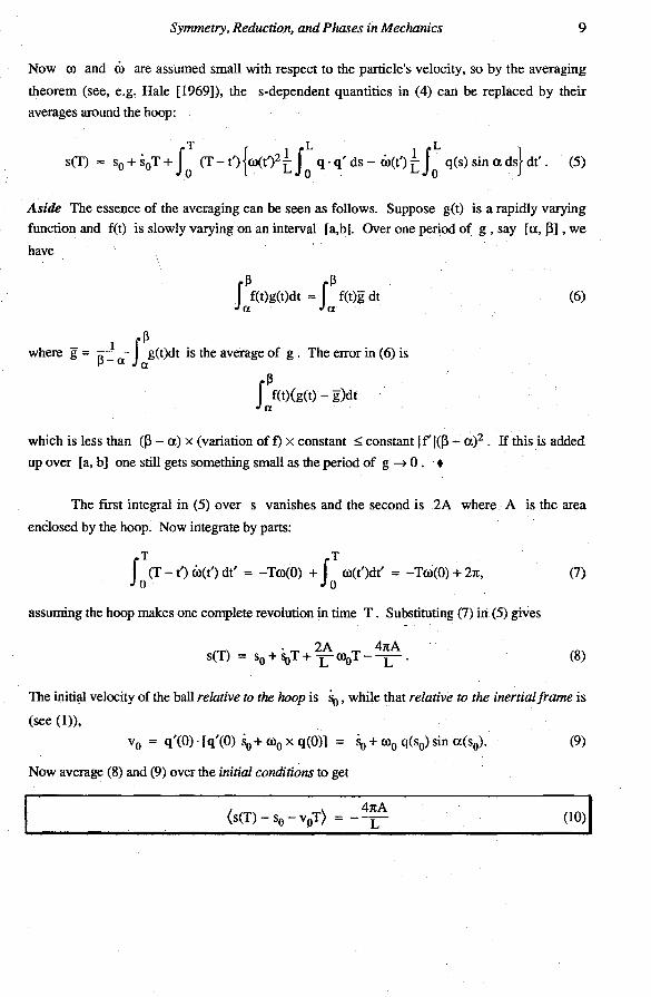
Now ro and ro are assumed small with respect to the particle's velocity, so by the averaging

theorem (see, e.g. Hale [1969]); the s-dependent quantities in (4) can be replaced by their

averages around the hoop:

. JT { 1 JL . 1 JL } seT) '" So + SoT + 0 (T - t') ro(t')2r:: 0 q. q' ds - ro(t') r:: 0 q(s) sin a ds dt'. (5)

Aside The essence of the averaging can be seen as follows. Suppose get) is a rapidly varying

function and f(t) is slowly varying on an interval [a,b]. Over one period of g, say [a, /3] , we

have

f3 f3 Lf(t)g(t)dt '" J

a f(t)g dt (6)

f3 where g = f3 ~ a J ag(t)dt is the average of g. The error in (6) is

f3 J af(t) (g(t) - g)dt

which is less than (/3 - a) x (variation of f) x constant ~ constant 1 f' 1(/3 - up. If this is added

up over [a, b] one still gets something small as the period of g ~ O. •

The first integral in (5) over s vanishes and the second is 2A where A is the area

enclosed by the hoop. Now integrate by parts:

T T J 0 (T - t') ro(t') dt' = - Tro(O) + J 0 ro(t')dt' = - Tro(O) + 21t, (7)

assuming the hoop makes one complete revolution in time T. Substituting (7) in (5) gives

(8)

The initial velocity of the ball relative to the hoop is So, while that relative to the inertial frame is

(see (1»,

(9)

Now average (8) and (9) over the initial conditions to get


which means that on average, the shift in position is by 4~A between the rotated and nonrotated

hoop. Note that if 010 = 0 (the situation assumed by Berry [1985]) then averaging over initial

conditions is not necessary. This process of averaging over the initial conditions that we naturally

encounter in this example is related to the recent work of Golin and Manni [1989] on experimental

procedures to measure the phase shift

This extra length 4~A is sometimes called the Hannay-Berry phase. Expressed in 2 '

angular measure, it is 81t /. In § llB we show, using the Cartan connection, how to realize this L

answer as the holonomy of the associated Hannay-Berry connection.

§lC Coupled planar pendula

We return now to an example similar to Elroy's beanie, with which we began. Consider

two coupled pendula in the plane moving under the influence of a potential depending on the hinge angle between them. Let r 1 ' r2 be the distances from the joint to their centers of mass and let 91

and 92 be the angles formed by the straight lines through the joint and their centers of mass

relative to an inertial coordinate system fixed in space, as in Figure IC-I. The Lagrangian of this

system is

and is therefore of the form kinetic minus potential energy, where the kinetic energy is given by the metric on ]R2 '

y

----------------Q-~--~------~x

Figure IC-I

To illustrate the ideas, we look at the special case II\ = ri =1 so that

and

The group Sl acts on configuration space ']['2 = {(91' 92)} by 9· (91' 92) = (9 + 91' 9 + 92)

so L is invariant under this action. Letting <P = (91 + 92)/...[2 and \jI = (91 - 92)1{2 , we see that

9· (<p, \jI) = (<p + 9, \jI) and hence that the induced momentum map for the lifted ~ction J: T*']['2

~ R is given by J(~, \jI, pep' pv) = Pep. Therefore the reduced space J-l(Il)/Sl is diffeomorphic

to T* S 1 = {('If, pv)} with the canonical symplectic structure. The Hamiltonian on T*']['2 is

H(<p, \jI, pep' pv) = ~ (p~ + p~) + V({2 \jI)

and the reduced Hamiltonian is

The equations of motion for H are

<p = Pep' P", = 0 (1)

\jf = Pv' Pv = - {2 v'C...[2 \jI) . (2)

Equations (2) are Hamilton's equations for HI! on the reduced space.

Assume that we have solved (2) with initial conditions ('lfo, pVo) and are given the initial

conditions (<Po' \jIo. Pepo = 11, pVo) of a solution for the system (1), (2). To find the solution for

(<p(t), \jI(t), Pep(t), pv(t» of (1), (2) we proceed in two steps:

Step 1 Consider the curve d(t) = (<Po' \jI(t), 11, pv(t».

Step 2 Solve the equation 9'(t) = 11, 9(0) = 0 yielding 9(t) = Ilt .

. Then the solution to (1), (2) is given by c(t) = 9·d(t) = (<po + Ilt, \jI(t), 11, pv(t».

This method is quite general and applies to all Hamiltonian systems. We will discuss it in

§2 and §3. To get a feeling of what is happening, we make some remarks. The principal

Sl-bundie J-1(1l) = {(<p, 'If, 11, pv)} ~ T*Sl , (<p, \jI, 11, pv) 1-7 ('If, pv) has a connection whose

horiwntal space at any point is generated by the vector fields {~ , ~}. Then the curve d(t) in ov oPv

Step 1 is simply the horizontal lift of the integral curve of the reduced system ('If(t), pv(t»

12 Marsden~ Montgomery, and Ratiu

through (<Po' '1'0,11, P'lfo)' Note that this connection on J-l (l1) ~ T*Sl is the pull-back of the

connection on 'f2 ~ Sl , (<p, '1') H '1', whose horizontal space at any point is generated by a~ ,

by the map which is the restriction of the cotangent bundle projection T*'f2 ~ 'f2 to J-1(11).

Relative to this connection and identifying T*'j['2 with TJ['2 using the kinetic energy metric ds2 = ,

dcp2 + dV2, 11 is. the generator of the vertical part of this curve; note II aiJcp 112 = II iJ~ 112 = 1.

Thus the differential equation in Step 2 is on the group Sl and has right hand side given by the

generator of the vertical part of the horizontally lifted curve in Step 1. Roughly, this describes

the method of reconstruction of dynamics. We shall explain this in §2 and address the

specific case of Lagrangian systems in §3, circumventing the use of the connection in Step 1.

UD Coupled bodies, linkages and optimal control

The above example can be generalized to the case of coupled rigid bodies. Already the case

of a single rigid body in space is an interesting example that will be discussed in §lG below. For

several coupled rigid bodies, the dynamics is quite complex. For instance for bodies in the plane,

the dynamics is known to be chaotic, despite the presence of stable relative equilibria. See Dh,

Sreenath, Krishnaprasad, and Marsden [1989]. Berry phase phenomena for this type of example

are quite interesting and are related to some of the work of Wilczek and Shapere on locomotion in

micro-organisms. (See, for example, Shapere and Wilczek [1987]). In this problem, control of the

system's internal variables can lead to phase changes in the external variables. These choices of

variables are related to the variables in the reduced and the unreduced phase spaces, as we shall

'see. In this setting one can formulate interesting questions of optimal control such as "when a cat

falls and turns itself over in mid flight (all the time with zero angular momentum!) does it do so

with optimal efficiency in terms of say energy expended?"


Figure ID-I

There are interesting answers to these questions that are related to the dynamics of Yang

Mills particles moving in the associated gauge field of the problem. See Montgomery [1989] and

references therein. This bundle approach to mechanics will be a theme developed in this work as

well.

We give two simple examples of how this works. Additional details will be given for this

type of example in §5. First, consider three coupled bars (or coupled planar rigid bodies) linked

together with pivot (or pin) joints, so the bars are free to rotate relative to each other. Assume the

bars are moving freely on the plane with no external forces and that the angular momentum is zero.

However, assume that the joint angles can be controlled with, say, motors in the joints. Figure

ID-I shows how the joints can be manipulated, each one going through an angle of 2n; and yet

the overall assemblage rotates through and angle n;. A formula for the reconstruction phase

applicable to examples of this type is given in Krishnaprasad [1989].

A second example is the dynamics of linkages; see §5E for more details. This type of

example is consideres in Krishnaprasad [1990], Yang and Krishnaprasad [1989], and

Krishnaprasad and Yang [1990], including comments on the relation with the three manifold


theory of Thurston. Here one considers a linkage of rods. say four rods linked by pivot joints as in

Figure ID-2. The system is free to rotate without external forces or torques, but there are

assumed to be torques at the joints. When one turns the small "crank" the whole assemblage turns

even though the angular momentum, as in the previous example, stays zero.

overall phase rotation of the assemblage

Figure ID-2

§ IE Quantum mechanics

The original motivation for geometic phases came from quantum mechanics. Here the

important contributions historically were by Kato in 1950 (for the quantum adiabatic theorem),

Longuet-Higgins in 1958 for anomalous spectra in rotating molecules, Berry [1984] who ftrst saw

the geometry of the phenomena for a variety of systems, and Simon [1983] who explicitly realized

the phases as the holonomy of the Chern-Bou connection. For more information on quantum

mechanical phases, and for the references quoted, see the collection of 'papers in Shapere and

Wilczek [1988].

For the purposes of the present work, the paper of Aharonov and Anandan [1987] plays an

important role. They got rid of the adiabaticity and showed that the phase for a closed loop in

projectivized complex Hilbert space is the exponential of the symplectic area of a two-dimensional

manifold whose boundary is the given loop. The symplectic form in question is naturally induced

on the projective space from the canonical symplectic form of complex Hilbert space (minus the


imaginary part of the inner product) via reduction, as in Abraham and Marsden [1978]. We shall

show in §4 that this formula is the holonomy of the closed loop relative to a principal SC

connection on complex Hilbert space and is a particular case of the holonomy formula in principal

bundles with abelian structure group.

Littlejohn [1988] has shown that the Bohr-Sommerfeld and Maslov phases of semi

classical mechanics can be viewed as incarnations of Berry's phase. To do this he notes that

Gaussian wave-packets define an embedding of classical phase space into Hilbert space, then uses

the Aharonov-Anandan point of view on phases, together with the variational formulation of

quantum mechanics. The quantum-classical relation between the phases is also considered in

Hannay [1985], Anandan [1988], and Weinstein [1989a,b].

§IF Integrable systems

Consider an integrable system with action-angle variables (11' 12, ... , ~, el' e2, ••. , en)

and with a Hamiltonian H(l1' 12, ••. In' el' e2, •.• en; m) that depends on a parameter m E M.

Let c be a loop based at a point IIlo in M. We want to compare the angular variables in the toms

over mo' once the system is slowly changed as the parameters undergo the circuit c. Since the

dynamics in the fiber varies as we move along c, even if the actions vary by a negligible amount,

there will be a shift in the angle variables due to the frequencies roi = dH!dli of the integrable

system; correspondingly, one defines

1

dynamic phase = f 0 roi(I, c(t))) dt .

Here we assume that the loop is contained in a neighborhood whose standard action coordinates

are defined. In completing the circuit c , we return to the same toms, so a comparison between the

angles makes sense. The actual shift in the angular variables during the circuit is the dynamic

phase plus a correction term called the geometric phase. One of the key results is that this

geometric phase is the holonomy of an appropriately constructed connection called the Hannay

Berry connection on the torus bundle over M which is constructed from the action-angle

variables. The corresponding angular shift, computed by Hannay [1985], is called Hannay's

angles, so the actual phase shift is given by

Ae = dynamic phases + Hannay's angles.

The geometric construction of the Hannay-Berry connection for classical systems is given in terms

of momentum maps and averaging in Golin, Knauf, and Marmi [1989] and Montgomery [1988].


In this paper we will put this geometry into a more general context and will synthesise it with our

work on connections associated with moving systems.

§lG The Rigid Body

The motion of a rigid body is a geodesic with respect to a left-invariant Riemannian metric

(the inertia tensor) on 80(3). The corresponding phase space is P = T*80(3) and the momentum

map J : P ~ R3 for the left 80(3) . action is right translation to the identity. We identify so(3)*

with so(3) via the Killing form and identify R3 with so(3) via the map v H v where v(w) = v x w, x being the standard cross product. Points in so(3)* are regarded as the left reduction of

T*80(3) by 80(3) and are the angular momenta as seen from a body-fixed frame. The reduced

spaces J-1(Il)!GI! arddentified with spheres in R3 of Euclidean radius If 11 If, with their

symplectic form wI! = - dS 1/111/1 where dS is the standard area form on a sphere of radius /111/1

and where GI! consists of rotations about the Il-axis. The trajectories of the reduced dynamics

are obtained by intersecting a family of homothetic ellipsoids (the energy ellipsoids) with the

angular momentum spheres. In particular, all but at most four of the reduced trajectories are

periodic. These four exceptional trajectories are the well known homoclinic trajectories. Suppose a reduced trajectory Il(t) is given on P /!' with period T. After time T, by how

much has the rigid body rotated in space? The spatial angular momentum is 1t = 11 = gIl, which is

the conserved value of J . Here g E 80(3) is the attitude of the rigid body and II is the body

angular momentum. If Il(O) = Il(T) then 11 = g(O)Il(O) = g(T)Il(T) and so g(T)-lll = g(O)-lll

i.e., g(T)g(O)-l is a rot~tion about the axis 11. We want to compute the angle of this rotation.

To answer this question, let c(t) be the corresponding trajectory in J-1(1l) C P. Identify

T*80(3) with 80(3) x R3 by left trivialization, so c(t) gets identified with (g(t), Il(t». Since

the reduced trajectory Il(t) closes after time T, we recover the factthat c(T) = gc(O) for some g

E Gw Here, g = g(T)g(O)-l in the preceding notation. Thus, we can write

g = exp[(8e)~] (1)

where ~ = III JIll n identifies g I! with JR. by a~ H a, for a E JR.. Let .D be one of the two

spherical caps on S2 enclosed by the reduced trajectory, A be the corresponding oriented solid

angle, i.e., IAI = (area D)//lIl/l2, and let HI! be the energy of the reduced trajectory. All norms

are taken relative to the Euclidean metric of JR.3. We shall prove below that modulo 21t, we have

89 = -- W + 2H T = -A + :::.:l!:.:. . 1 {J } 2H T 111111 D I! I! 111111

(2)


(The special case of this formula for a symmetric free rigid body was given by Hannay [1985] and

Anandan [1988], formula (20».

dynamic phase

holonomy (geometric phase)

0;..I0 __ ~

horizontal lift of reduced trajectory

~-]~educ{:d trajectory

1 J . 1 T Figure IG-l For Gil = Sl, (log holonomy) = 1IJ.l1I D 00

11, (log dynamic phase) = 1IJ.l1I J 0 ~(t) dt, where,

. T = period of reduced trajectory and 0011 = reduced symplectic form.

To prove (2), we choose the connection one-form on J-1(1l) to be (see Proposition 2.2)

1 A=-a

111111 Il (3)

where all is the pull back to J-1(1l) of the canonical one-form a on T*SO(3). The curvature of

A as a two-form on the base Pit' the sphere ofiadius 111111 in JR3, is given by

18 Marsden; Montgomery. and Ratiu

1 1 --00 =--dS.

II~II IL 1I~1I2 (4)

The first terms in (2) represent the geometric phase. i.e., the holonomy of the reduced trojectory

with respect to this connection. By Corollary 4.2, the logarithm of the holonomy (modulo 21t) is

given as minus the integral over D of the curvature, i.e., it equals

1 J 1 - 00 = - -- (area D) = -A (mod 21t) II~II D IL 1I~1I2

(5)

The second terms in (2) represent the dynamic phase. By the algorithm of Proposition 2.1 it is calculated in the following way. First one horizontally lifts the reduced closed trojectory rI(t)

to J-l(~) relative to the connection (3). This horizontal lift is easily seen to be (identity, rI(t» in

the left trivalization of T~80(3) as 80(3) x]R3. Second, one computes

~(t) = (A· XH)(rI(t» .

Since in coordinates

~. ~ . d d 8 = £.. Pi dq' and XH = £.. p'-. + - terms

IL i i dq' dP

for pi = l gijpj• gij being the inverse of the Riemannian metric gij on 80(3). we get J

(81L

·XH)(rI(t» = lPipi = 2H(identity, rI(t» = 2HIL , 1

where HIL is the value of the energy on S2 along the integral curve rI(t). Consequently.

t _ 2HIL ~() - II~II ~

Third, since set) is independent of t, the solution of the equation

2HIL g = gS = II~II g~ is (

2H t ) get) = exp =:g:. ~ II~II

so that the dynamic phase equals

2H ~e =::.:I!: T (mod 21t)

d II~II

(6)

(7)

(8)

(9)

Formulas (5) and (9) prove (2). Note that (2) is independent of which spherical cap one chooses

amongst the two bounded by rI(t). Indeed, the solid angles on the unit sphere defined by the two

caps add to 41t, which does not change formula (2).

~2 Reconstruction of Dynmnics for Hamiltonian Systems

This section presents a reconstruction method for the dynamics of a given Hamiltonian

system from that of the reduced system. The method and formulas found here are applied in the

next section to Lagrangian systems.

§2A General Considerations

We begin with the abstract reconstruction method. Let P be a Poisson manifold on which

a Lie group acts in a Hamiltonian manner and has a momentum map J: P ~ g*; -here 9 is the

Lie algebra of G and g* is its dual. For a weakly regular value 11 E g* of J, assuming that

the reduced space P 11 : = J-1 (1l)/G 11 is a smooth manifold with the canonical projection a

surjective submersion, PIl a Poisson manifold (see Marsden and Ratiu[1986] for the general

theory of Poisson reduction). Given f, h: P 11 -+lR, lift them to J-1(1l) by 1t1l

, then extend

them to G-invariant functions on J-1( 0Il)' where 0Il is the coadjoint orbit of 11 in g*, and

then extend these functions arbitrarily to f, h: P ~ R The Poisson bracket of f and h in the

Poisson structure of P 11 is defined by {f, h} 01t1l

= {f I 0Il' h lOll}' If P is symplectic, then P 11

is also symplectic (see Marsden and Weinstein [1974] and Abraham and Marsden [1978], Chapter 4). If H : P ~ lR is a G-invariant Hamiltonian it induces a Hamiltonian HIl : P 11 ~ lR and the

flow of the Hamiltonian vector field XH on P 11 is the Gil-quotient of the flow of XH on J-1(1l).

" Assume that an integral curve cll (t) of XH on P 11 is known. For Po E

" -J-1(1l), we search for the corresponding integral curve c(t) = Ft(po) of XH such that 1t

1l(c(t» =

cll(t), where 1t1l

: J-1(1l) ~ P 11 is the projection. Pick a smooth curve d(t) in J-1(1l) such that

d(O) = Po and 1t1l (d(t» = cll (t). Write c(t) = <D g(t)(d(t» for some curve get) in Gil to be

determined. We have

Since <D;XH = X <t>*H = XH ' (1) gives g

This is an equation for get) written in terms of d(t) only. We solve it in two steps:

19

Step 1 Find ~(t) E gil such that

Step 2 With ~(t) determined, solve the non-autonomous ordinary differential equation on GIL:

g'(t) = TeLg(t)(~(t»), with g(O) = e.

Step 1 is typically of an algebraic nature; in coordinates, for matrix Lie groups, (3) is just a matrix

equation. We show later how ~(t) can be explicitly computed if a connection is given on J-l(J.I.)

~ P W Step 2 gives an answer "in quadratures" if G is abelian as we shall see in formula (5)

below. In general (4) cannot be solved explicitly and represents the main technical difficulty in the

reconstruction method. With get) determined, the desired integral curve c(t) is given by c(t) =

<D g(t)(d(t». The same construction works on PIG, even if the G-action does not admit a

momentum map ..

Step 2 can be carried out explicitly when G is abelian. Here the connected component of the identity of G is a cylinder lRP x Tk-p and the exponential map exp(~l' ... , ~k) = (~l' ... , ~, ~P+l (mod 2n), ... , ~k(mod 2n» is onto, so we can write get) = exp T](t), T](O) = O. Therefore

~(t) = Tg(t)L _l(g'(t») = T]'(t) since T]' and T] commute, i.e., T](t) = Jot ~(s)ds. Thus the g(t)

solution of (4) in Step 2 when G is abelian is

get) = exp U; ~(s)ds ) (5)

This reconstruction method depends on the choice of d(t). With additional structure, d(t)

can be chosen in a natural geometric way. What is needed is a way of lifting curves on the base of

a principal bundle to curves in the total space. We do this using connections. One can object at this

point that at the moment, reconstruction involves integrating one ordinary differential equation,

whereas introducing' a connection will involve integration of two ordinary differential equations,

one for the horizontal lift and one for constructing the solution of (4) from it. However, for the

determination of phases, there are some situations in which the phase ca:n be computed without

actually solving either equation, so one actually solves no differential equations; a specific case is

the rigid body, discussed in §lG. In other circumstances, one can compute the horizontal lift

explicitly (see Marsden, Ratiu, and Raugel [1990]). However, in general, without such added

information,it is true that the number of equations in principle is two rather than one. Suppose that nil: J-1(1l) ~ PIl is a principal Gil-bundle with a connection A. This

means that A is a gil-valued one-form on J-1(1l) c P satisfying


ii L*A=Ad 0 A g g

Let d(t) be the horizontal lift of cll

through Po; i.e., Ad'(t) = 0, 1t1l 0 d = cll ' and d(O) =

Po'

2.1 Theorem Suppose 1t1l

: J-10l) ~ P Il is a principal Gil-bundle with connection A. Let

cll

be an integral curve of the reduced dynamical system on P w Then the corresponding curve c

(through Po E 1t~l(cll(O») of the system on P is determined asfollows:

Horizontally lift cll

to form the curve d in J-1(1l) through Po'

i i Set ~(t) = fit . XH(d(t», so that ~(t) is a curve in gw

iii Solve the equation get) = g(t)· ~(t).

Then c(t) = g(t)·d(t) is the integral curve of the system on P with initial condition Po'

Suppose cll

is a closed curve; thus, both c and d reintersect the same fiber. Write

d(l) = g . d(O) and c(1) = h· c(O)

for g, h E Gil' Note that h = gel) g . (6)

The Lie group element g (or the Lie algebra element log g) is called the geometric phase. It is

the holonomy of the path cll

with respect to the connection A and has the important property of

being parametrization independent. The Lie group element gel) (or log g(l» is called the

dynamic phase. For compact or semi-simple G, Gil is generically abelian. The computation of g(1) and

g are then relatively easy, as was indicated above.

§2B Cotangent Bundle with G Ii one Dimensional

We now discuss the case in which P = T*Q, and G acts on Q and therefore on P by

cotangent lift. In this case the momentum map is given by the formula

where ~ E gil' uq E T~Q, e = LPi dqi is the canonical one-form and -.l is the interior product. i


Assume GIL is the circle group or the line. Pick a generator ~ E gil' ~"# O. For

instance, one can choose the shortest ~ such that expC21t~) = 1. Identify gIL with the real line

via co ~ ro~. Then a connection one-form is a standard one-form on j-1C/-L).

2.2 Proposition Suppose GIL == S1 or R Identify gIL with lR via a choice of generator

~. Let ell denote the pull-back of the canonical one-form to j-1C/-L). Then

1 A=--e ®~

(/-L,~) Il

is a connection one-form on j-1C/-L) ~ Pit" Its curvature as a two-form on the base P Il is

where roll is the reduced symplectic form onP It"

Proof Since G acts by cotangent lift, it preserves e, and so ell is preserved by GIL and

therefore A is GIL-invariant. Also, A~p = [~p -' e / (/-L, ~)]~ = [j~/(/-L, ~)]~ = ~. This

verifies that A is a connection. The calculation of its curvature is straightforward. (See §4 and note that ro = - de in our conventions.) _

Remarks 1 The result of Proposition 2.2 holds for any exact symplectic manifold. We shall

use this in §5A. 2 In the next section we shall show how to construct a connection on j-1(/-L) ~ P Il

in general. For the case Q = G it includes the connection in 2.2. For Q = 80(3) this recovers

the connection for the rigid body. We will return to this point shortly.

§2C Cotangent Bundles - General Case

If GIL is not abelian, the formula for A given above does not satisfy the second axiom of

a connection. However, if the bundle Q ~ QlGIl has a connection, we ~ill show below how this

induces a connection on j-1(/-L) ~ (T*Q)1t" To do this, we recall the cotangent bundle reduction

theorem of Satzer, Marsden and Kummer (see Abraham and Marsden [1978], §4.3 and Kummer

[1981]).

Assume the Lie group G acts freely on the left on Q; lift this to a symplectic action on

T*Q. The momentum map of this lift is j(aq).~ = aq·~Q(q), where a q E T~Q, ~ E g, and

~Q(q) = !I £=0 (exp e~'q) is the infinitesimal generator of the G-action on Q defined by S·

Assume that ~ is a weakly regular value and that J-l(~)/G~ = (T*Q)~ is a smooth manifold and

that the canonical projection 1t~: J-l(~) ~ (T*Q)~ is a surjective submersion. Let g~ = {11 E

g 1 (ad 11)*~ = O} be the isotropy Lie algebra at ~; i.e., the Lie algebra of Gw and denote by 11'

= (~I g~) E g:, the restriction of ~ to g~. Assume that p~: Q ~ Q/G~ is a principal bundle

and Y E Ql(Q; g~) is a left connection one-fonn on Q, i.e., "«11Q) = 11 for all 11 E g~ and 'Y

is G~-equivariant: Yg.q(g ·v) = Adl"{(v» for all g E Gw q E Q, V E TqQ~

2.3 Theorem Let curv(y) be the curvature of Y and let B be the pull-back by the cotangent

bundle projection T* (Q/G~) ~ Q/G~ of the two form on Q/Gil induced by the 11' -component

~'·curv(y) E Q2(Q) of curv(y); thus ~'·curv(y) is a closed real-valued Molom! on Q and B

is a closed two-form on T* (Q/GIl). Endow T*<Q/G~) with the symplectic form ro - B, where

(J) is the canonical twolorm of the cotangent bundle. Then (T*Q)~ is symplectically embedded in

(T*(Q/GIl), ro - B) and its image is a vector subbundle with base Q/Gw This embedding is onto

if and only if g = gw

Denote by J~: T*Q ~ g: the induced momentum map, i.e., JIl(uq) = J(uq) I g~ . From

the proof of the theorem, which is ultimately based on a momentum shift in the fiber, it follows

that this diagram commutes:

(T*Q)~ -----------"'.-'T*(Q/GIl) - Q/G~

[uqJ 1 • [uq -~" Yl)] 1-1 --------- [q]

where tiUq) = u q - ~"Yl') is fiber translation by the ~'-component of the .connection fonn and

where [uq - ~"Yq(-)] means the element of T*(Q/GIl

) detennined by u q - ~'·YqC). Call the

composition of the two maps on the bottom of this diagram (J: [uq] E (T*Q)1l H [q] EQ/G~ . A


natural way of inducing a connection on J-1(1l) ~ (T*Q)1l is to be consistent with this theorem,

i.e., by pull-back in the diagram above.

2.4 Corollary The connection onejorm yE Q1(Q; gil) induces a connection onejorm yll

E Q1(r1(1l); gil) by pull-back: yll = (1t 0 tll)*y , i.e.,

Similarly curvcYll) = (1to til) * cUIV(y) and in particular the Il'-component of the curvature of this

connection equals B, the pull-back of Il'·curv(y).

The proof is a direct verification.

2.5 Corollary Assume that PIl : Q ~ Q/GIl

is a principal Gil-bundle with a connection y E

Q1(Q; gil). If R is a G-invariant Hamiltonian on T*Q inducing the Hamiltonian HIl on

(T*Q)1l and ca(t) is an integral curve of XH ' denote by d(t) a horizontal lift of ca(t) in J!

J-1(1l) relative to the natural connection of Corollary 2.4 and let q(t) = 1t(d(t» be the base

integral curve of c(t). Then set) of step ii in Theorem 2.1 is given by

set) = y(q(t»-FH(d(t»),

where FH: T*Q ~ TQ is the fiber derivative of H, i.e., FH(uq)·/3q = ~I t=O H(uq + t/3q).

If Q carries a G-invariant Riemannian metric «,» define an associated connection Ymech

E Q1 (Q; gil) by declaring the horizontal space at any q E Q to be the orthogonal complement of

the vertical space. Assume also that the Hamiltonian H is of the form kinetic energy with respect

to the metric ((,» plus a G-invariant potential energy.

2.6 Corollary Under these hypotheses, step iiin Proposition 2.1 is equivalentto ii'S(t) E gil is given by

set) = Ymech(q(t»·d(t)#, where d(t) E T~(tP.

Proof Apply Corollary 2.4 and use the fact that FH(u) = u#. (In coordinates, aaR = gllVpv ). q q ~

•


In this case, 'Ymech is closely related to the mechanical connection that appears in the

work of Smale [1970], Guichardet [1984], Wilczek and Shapere [1988], Montgomery

[1988,90a,b], Lewis, Marsden, Simo and Posbergh [1989] and Simo, Lewis and Marsden

[1989]. It is given explicitly as follows: let ~(q): g!J. ~ g; be defined by ][!J.(S)(ll) = (SQ(q),

llQ(q» be the J.!-locked inertia tensor. This name is used because for coupled rigid (or rigid

flexible) structures, ][!J. (q) is the inertia tensor of the system with the joints locked in the

configuration q, thereby forming a rigid body. Then 'Ymech: TQ ~ g!J. is

where vqb is the one-form corresponding to the vector Vq via the metric. Shapere and Wilzcek

call this the "master formula".

Besides choosing the connection 'Ymech to be defined by the metric orthogonal to the G!J.

orbits, one can use other complements. Here is one such:

2.7 Corollary If Q = G, dim G!J. = 1, and S is a generator of g!J.,' the one-form 'YR E

Ql(G) given by

( ) - _l-T*R () 'YR g - (J.!, S) g g-l J.!

induces via the procedure in Corollery 2.4 the connection A E Ql(J-C(J.!)) given in Proposition

2.2, where JL(ug) = T:Rg(Ug). Here, (J.!, S) is the naturaipairing between J.! and S·

Proof The axioms of a left principal G!J.-connection, namely 'YR(Sa) = S and'YR(hg)(Tg~(vg))

= 'YR(g)(v g) for all hE Gg and v gET gG are straightforward-verifications; recall that Sa (g) =

TeRg(S)' Moreover, for ug E J-C(J.!) and UUg

E TUg (J-C(J.!», we have

~3 Reconstruction of Dynamics for Lagrangian Systems

In this section we reconstruct the dynamics of a given Lagrangian system with symmetry

from the reduced dynamics. We begin by recalling the basic facts about Lagrangian systems.

§3A Lagrangian Systems

If Q is a manifold, L: TQ -t R is a smooth function, and 't : TQ -t Q the projection, let

lFL : TQ -t T*Q be the fiber derivative of L given by

lFL(v) . w = .Q.I L(v + lOW), dE 10=0

for v, w E TqQ. If Q denotes the canonical symplectic structure on T*Q, let QL = (lFL)*Q, a

closed two form on TQ. If QL is a (weak) symplectic form, we call L regular. In local charts

this is equivalent to the second derivative in the fiber variable to be a (weakly) non-degenerate

bilinear form. If lFL is a diffeomorphism, L is called hyperregular and lFL the Legendre

transformation. Returning to a general Lagrangian L, let A(v) = lFL(v)· v be the action of

Land E = A - L the energy of L. A vector field Z E X(TQ) is called a Lagrangian

system, if iZQL::::; dE, where iz denotes the interior product (or contraction) with Z. If L is

regular, then Z is a second order equation, i.e., T't 0 Z = identity on TQ, where 't : TQ -t Q is

the tangent bundle projection. In general, if we assume that Z is second order, then locally

Lagrange's equations hold:

where q(t) = dq(t)/dt and Dl and D2 denote the partial Frechet derivatives. Moreover, E is

conserved by the flow of Z. In this section we will assume that Z isa second order equation. If L is hyperregular, then Z = X E is the Hamiltonian vector field relative to QL defined

by E. Then H = Eo (lFL)-l : T*Q -t R defines a Hamiltonian system XH on T*Q whose flow

is conjugate by lFL to that of XE on TQ. The fiber derivative lFH: T*Q -t TQ of H (defined

in Corollary 2.5) is the inverse of lFL. Conversely, if H: T*Q -t R is hyperregular. i.e., lFH:

T*Q -t TQ is diffeomorphism, let e(XH) be the action of H, where e is the canonical one

form on T*Q. Our convention is Q = -de. Let A = e(XH) 0 (lFH)-l, E = H 0 (lFHtl, and L =

26


A-E. Then L is the Lagrangian system inducing H and the above prescription defines a

bijective correspondence between hyperregular Lagrangians on TQ and hyperregular

Hamiltonians on T*Q. Moreover, the base integral curves (i.e., the projections of the integrals

curves on TQ and T*Q onto Q) of XE and XH coincide. See, e.g., Abraham and Marsden

[1978] for the proofs.

Let a Lie group G act on Q and that L is invariant under the lifted G-action to TQ. The

Legendre transformation lFL is equivariant relative to this action and the cotangent lifted action on

T*Q, and so A, E, QL' and Z are G-invariant. Assuming that (TQ)/G is a smooih manifold

with the projection p: TQ ~ (TQ)/G a surjective submersion, E induces a smooth function EG

and Z a smoothvectorfield ZG on (TQ)/G; the flow of ZG conserves EG. The question we

shall address in this section is the following: given an integral curve cG(t) of ZG' coCO) = [Vq]

and Vq E T qQ, construct the integral curve c(t) of Z satisfying c(O) = v q.

§3B Reconstruction for Q = G

We begin with the simplest case: Q = G with a left-invariant Lagrangian L: TG ~ JR.,

L(TgLh(Vg» = L(vg), where h, g E G, Vg E TgG, ~: G ~ G denotes \eft-translation by h,

~(k) = hk, and Tg~: Tp ~ ThgG is its tangent map.

3.1 Proposition Let L: TG ~ JR. be a left-invariant Lagrangian such that its Lagrangian

vector field Z E X(TG) is a second order equation. Let ZG E X( g) be the induced vector field

on (TG)/G '" 9 and let ~(t) be an integral curve of Zo. If get) EGis the solution of the non

autonomous ordinary differential equation get) = TeLg(t)~(t), g(O) = e,and g E G then vet) = TeLgg(t)~(t) is the integral curve of Z satisfying v(O) = TeLg ~(O) and vet) projects to ~(t),

i.e., TL't(v(t»-1 vet) = ~(t).

Proof Let vet) be the integral curve of Z satisfying v(O) = TeLg~(O) for a given element ~(O)

E g. Since ~(t) is the integral curve of Za whose flow is conjugated to the flow of Z by left

. translation, we have TL't(v(t»-1 vet) = ~(t). If h(t) = 't(v(t», since Z is a second order equation,

we have

vet) = h(t) = Te~(t) ~(t) and h(O) = 't(v(O» = g

so that letting get) = g-lh(t) we get g(O) = e and

This determines get) uniquely from ~(t) and so


In general, Za is not Hamiltonian. However, if L is hyperregular, then the Legendre

transformation FL will induce a Poisson structure on g. In fact, in this case, we can reconstruct

the dynamics of the induced Hamiltonian system.

3.2 Corollary Let L: TG ~ JR be a left-invariant hyperregular Lagrangian, H: T*G ~ JR

the induced Hamiltonian, and h: g~ ~ JR the induced Hamiltonian on the dual g * of g

endowed with the Lie-Poisson structure; h = HI g*. Let Il(t) be an integral curve of X h(ll) =

ad (~~)* 11, 11(0) = T!Lg(Ug), u g E G fixed. If ~(t) = (JF1L)-lll(t) and g(t) is the solution of

. . * * g(t) = TeLg(t) ~(t), g(O) == e, then u(t) = T L(gg(t))-IIl(t) is the integral curve of X H on T G,

a(O) = u g and u(t) projects to Il(t),i.e., T!L1t

(a,(t)) = Il(t); 1C: T*G ~ G denotes the cotangent

bundle projection.

The proof is a consequence of the previous result and the fact that FL commutes with left

translation: FL 0 TLg = T*Lg -I 0 FL.

§3C General Q

In §3B we studied reconstruction for the case of Lie-Poisson reduction for a given

invariant Lagrangian. In the general case, instead we take a symplectic reduction viewpoint. Given

is L: TQ~ JR, G-invariant, Z E X«TQ) its Lagrangian vector field which we assume to be a

second order equation. The lift of the G-action to TQ induces an equivariant momentum map J:

TQ ~ g* given by

(1)

for Vq E TqQ, ~ E g. Let 11 E g* be a weakly regular value of J apd assume that PIl : Q ~

QlGw TQ ~ (TQ)/GIl

are principal GIL-bundles, where GIL is the co adjoint isotropy group at

11. By conservation of J, GIL acts on J-1(1l) so we can form the reduced space (TQ)1l = J-1(Il)/GW Given is v q E J-1 (11) and an integral curve cit) of the induced vector field ZIl E

X«TQ)Il)' cll(O) = [vq]; we want to explicitly find the integral curve c(t) satisfying c(O) = vq.

For this purpose we formulate the tangent bundle version of Theorem 2~3 of the previous section.


3.3 Proposition Let IJ.' = IJ.I gJ.1 and JJ.1: TQ ~ g: be given by JJ.1(vq)·11 = lFL(v)·11Q(q)

for all 11 E gJ.1" Assume that there is a vector field Y J.1 E £(Q) such that Y J.1 (Q) C (JI1)-l(IJ.') and

Y J.1 is G-equivariant: Y J.1(g.q) = g·Y J.1(q). Then there is an embedding Cj>J.1: (TQ)J.1 = J-l(IJ.)/GI1 ~ T(Q/GJ.1) whose range is a vector subbundle with base QlGJ.1" This embedding is onto if and

only if g = gil" If L : TQ ~ lR is a G-invariant Lagrangian whose Lagrangian vector field Z E

£(TQ) is a second order equation, let c(t) denote an integral curve of Z and let q(t) = 't(c(t» be

the corresponding base integral curve, where 't: TQ ~ Q is the tangent bundle projection. Let

CJp.(t) = PJ.1(q(t» be the corresponding curve in QlGJ.1 and Y J.1 E £«QlGJ.1) the vectorfield induced

by YJ.1" Then the intelJral curve cit) of ZJ.1 covered by c(t) is Cj>~l(q~(t) - Yiqit))). The

curve qit) is the image of cJ.1(t) by Y J.1 followed by the projection T(QlGJ.1} ~ QlGJ.1"

Proof The fIrst part of the proof is a restatement of the standard proof of Theorem 2.3. Indeed,.

Y J.1 induces, by equivariance, the vector fIeld Y J.1 on QlGJ.1: Y J.1 0 PJ.1 = TPI1 0 Y J.1"DefIne the

projection 'til: (TQ)11 ~ Q/GI1 by 't11([vq]) = [q], so that PI1 0 't = 'til 0 1tJ.1' where, as usual, 1t11 :

J-l(lJ.) ~ (TQ)J.1 is the canonical projection. Let ~: (JJ.1)-l ~ (F)-l(O) be given by ~(v q) = v q

Y J.1(q) and let Cj>J.1: (TQ)J.1 ~ T(QlGJ.1) be the induced map, Cj>11 0 1t11 = TPI1 o~, defIned on the set

J-l(IJ.). Then Cj>11 is an embedding and it is easy to see that it is onto iff, g = gJ.1 by comparing

(JI1)-l(O) with J-l(O).

For the second part, let cl1(t) = 1t11(c(t» be the integral curve of ZI1 covered by c(t). Then

qit) = PI1(q(t» = (pl1 0 't)(c(t» = ('tJ.1 0 1t11)(c(t» = 'tJ.1(cit». Let us show that q~(t) - Yiqit» is

in the range of Cj>J.1" We have

q~(t) - Y J.1(qit» = Tpiq'(t» - q~(t) - Y l1(p/q(t»

= TpJ.1(q'(t» - TPI1(Y l1(q(t» = TPI1(q'(t) - Y l1(q(t))).

Since Z is a second order equation, q'(t) = c(t). By conservation of J, c(t) E J-l(lJ.) for all t,

so q'(t) - Y iq(t» = Vq'(t» and thus

Therefore, the integral curve cit) covered by c(t) equals cl1(t) = Cj>'~{q~(t) - YJ.1(q/t») and the

proposition is proved. _

In general, Zjl. is not a second order equation. However, its integral curves are still

uniquely determined by the corresponding base integral curves i.e., by their projections on QlGw We next tum to the question of reconstruction of dynamics. We are given a base integral curve ~(t) of Zjl. determined by the initial conditions ~(O) and ~(O) and an equivariant vector field

Yjl. with values in (Jjl.)-1 (V), implementing the embedding of (TQ)jl. into T(QlGjl.)' We want to

reconstruct the integral curve c(t) = q'(t) of Z covering cit) = <p~1(qjl.(t) - Yjl.(qit))). For this

purpose, let "(E Q1(Q; gjl.) be a connection for the principal Gjl.-bundle Pjl.: Q -? QlGW Horizontally lift ~(t) to a curve qh(t) in Q with qh(O) = q(O):

(2)

for Vq E TqQ .and Vv E Tv (TQ). (Note that if L is hyperregular, i.e., lFL: TQ -? T*Q is a q q

diffeomorphism, then (lFL)* yjl. = "t, for yjl. the connection given in Corollary 2.4). In Step i of the reconstruction procedure we horizontally lift cjl.(t) to a curve d(t) in J-1(1l) with d(O) = c(O): 1tjl.(d(t» = cjl.(t) and "t(d(t» . d'(t) = O. To determine d(t), we begin by showing that

t(d(t» = qh(t). Indeed, t(d(t» covers qjl.(t): pjl.(t(d(t))) = (tjl. 0 1tjl.)(d(t» = 1tjl.(cit» = qjl.(t).

Moreover, since (t 0 d)'(t) = Tt(q'(t», the horizontality condition on d(t) becomes y(t(d(t»·(to

d)'(t) = 0, i.e, t(d(t» is horizontal. Finally, since t(d(O» = t(c(O» = q(O) = qh(O), the equality

t(d(t» = qh(t) follo~s by uniqueness of horizontal lift.

Next, we show that qh(t) is the 'Y-horizontal part of d(t). Indeed, since 1tjl.(d(t» = cfL(t) =

<p~1(q~(t) - Y jl.(qfL(t») by Proposition 3.3, we have

whence

~(t) - Y jl.(qfL(t» = (<PfL 0 1tfL)(c(t» = (<pjl. 0 1tfL)(d(t» = (TpfL 0 tfL)(d(t»

= TPjl.(d(t) - Yjl.(qh(t») = TpfL(d(t» - Y fL(piqh(t»)

= TpfL(d(t» - Y fL(~(t»,

q~(t) = TPfL(d(t».

Since Tpjl.(q~(t» = q~(t), it follows that d(t) - q~(t) is vertical, so q~(t) is the horizontal part of

d(t) and thus there is a unique ~(t) E gfL such that

(4)


Note that S(O)Q(q) is the vertical part of the initial condition v q. The only remaining condition on

d(t) is that it lie in J-1(1), i.e., that

(5)

for all 11 E g . This condition uniquely determines S(t) by the formula S(t) = -y(qh(t»)-d(t). We

have proved the following:

3.4 Corollary Under the hypotheses and notations of Proposition 3.3, let ~(t) be the base

integral curve of ZIL E X«TQ)IL) with initial conditions qlL(O), q~(O) and clL(t) == q>1(q~(t) -

Yi~(t») the corresponding integral curve of ~. Let 'YE n1(Q; gIL) be a connection on the

principal GIL-bundle PIL

: Q ~ Q/Gw Then the integral curve c(t) = q'(t) of Z E X(TQ)

covering clL(t) with initial condition Vq E ~l(clL(O» isfound in the following way:

horizontally lift ~(t) to a curve qh(t) in Q, qh(O) = q;

i i determine S(t) E gIL from the system

for all 11 E g; this implies that the horizontal part of the initial condition Vq is q~(O)

and the vertical part is S(O)Q(q);

iii solve the non-autonomous ordinary differential equation g'(t) = TeLg(t)S(t) with initial

condition g(O) = e on the Lie subgroup GW Then the base integral curve q(t) of Z with initial conditions q(O) = q, q'(O)::: v q is given by

q(t) = g(t)·qh(t) and the integral curve of Z with initial condition v q is q'(t) = g(t)·(q~(t) +

S(t)Q(qh(t»).

The vector field Y IL E X(Q) postulated in the hypotheses of Proposition 3.3 can be

chosen consistent with the connection 'f given by (3). Namely, derme

Y ig) = lFL(Il'·'Y(g», (6)

i.e., Y lL(g) is the Legendre transform of the Il'-component of the connection 'Y E Ql(Q; gIL)·

This choice for hyperregular Lagrangians (i.e., if lFL is a vector bundle isomorphism between

TQ and T*Q) allows one to pass freely between the Lagrangian and Hamiltonian point of views

both at the unreduced and reduced levels. We shall use this remark in §4D.


§3D Simple Mechanical Systems

To specialize this corollary to the case of Lagrangians of kinetic minus potential type, let

(Q, (,» be a Riemannian manifold with positive definite, G-invariant metric (,) and let V: Q

~lR bea G-invariantpotential. Then the classical Lagrangian L(vq)=!lIvqIl2-V(q) is G

invariant. The metric induces a principal connection on PIL : Q ~ Q/GIL by declaring the

horizontal subbundle to equal the orthogonal complement of the vertical subbundle. The condition detennining ~(t) E gIL becomes

(1)

for all 11 E g. Condition (1) implies that q~(O) is the horizontal part and ~(O)Q(q) the vertical

part of the initial condition Vq E TqQ. Split g = gIL E9 E for some complement E of gIL" Ifin

(1) 11 is taken to lie in gli' then by the defmition of the connection,

(2)

for all 11 E gIL' an equality uniquely detennining ~(t)Q('lb(t» for every t, and hence by freeness

of the GIL-action, uniquely determining ~(t) E gIL" There are still dim G - dim GIL equations to

be satisfied; these hold automatically by the previous corollary. We have thus proved the

following:

3.5 Corollary In the hypotheses of Proposition 3.3, let L(v q) =! II v q 112 - V(q), where

( ,) is a G-invariant positive definite Riemannian metric on Q and V : Q ~ lR is G-invariant.

Let Z E ,*(TQ) be the Lagrangian vector field of L and let ZI! E ,*«TQ)IL) be the induced

vector field on the reduced space. Let v q E J-l(~) and let qlL(t) be the base integral curve of ZIL

with initial conditionsltlL(vq). Then the integral curve c(t) of Z with initial condition c(O) = Vq

isfound in thefollowing way: endow the principal GIL-bundle PIL : Q ~ Q/GIL with the connection 'Ymech whose

horizontal subbundle is the orthogonal complement relative to (,) of the vertical

subbundle; ii horizontally lift qlL(t) to a curve qh(t) in Q satisfying qh(O)= q;

iii determine ~(t) E gIL from the algebraic system (~(t)Q(qh(t», 11Q(qh(t») = WTl for all

11 E gIL; this implies that q~(O) and ~(O)Q(q) are the horizontal and vertical parts of

the initial condition v q ;

iv solve the non-autonomous equation g'(t) = TeLg(t) ~(t), g(O) = e in GIL'

Then q(t) = g(t)·<ht(t) is the base integral curve of Z with initial conditions q(O) = q, q'(O)= Vq

and c(t) = q'(t) = g(t)·(q~(t) + ~(t)Q(qh(t») is.!he integral curve of Z with initial conditon c(O) =

vq•

It is easy to check that the Legendre transfonn of c(t) gives the integral curve of the

associated Hamiltonian system as obtained in 2.1 relative to the connection in 2.6.

There are several important situations when step ivcan be carried out explicitly. a If Gil is abelian, the equation g'(t) = TeLg(t) ~(t), g(O) = e, has solution w.ven by get)

= exp J; ~(s)ds. If Gil = SI, ~(s) can be explicitly determined from condition iii and hence the

reconstruction method 'bf Corollary 3.5 has an explicit solution. Indeed, if we denote by ~ E gil

a generator of gil' then (a(t)~)Q = a(t)~Q' so that by ii we get l.l:~ = (a(t)~Q(qh(t», ~Q(qh(t») = aCt) II ~(qh(t» IF and hence '

aCt) = 1.1. • ~ 2'

II ~Q(qh(t» II

Thus writing get) = exp(6(t)~), the solution of the equation in iv is given by

3.6 Corollary Let (Q, ( ,» be a Riemannian manifold with a G-invariant metric and V: Q

~ R be a G-invariant function. Assume Gil equals SI or R and let ~ be a generator of

gil' If Vq E J-l (ll) = {u E TQ I (u, ~Q(q) ) = Il'~} and qll is the base integral curve of the

induced vector field Z!l E X«TQ)Il) with initial conditions 1t1l

(vq), the base integral curve and

solution of the Lagrangian vector field Z given by L(vq> = ~ Itvqll2- V(q) with initial condition

v is given by

were

and qh(t) is the horizontal lift of ~(t) satisfying qh(O) = q.

b A second case in which the equation g'(t) = TeLg(t) ~(t) can be solved, even if Gfl is

non-abelian when ~(t) = ~(O) = ~ is constant. Theng(t) = exp(t~) is the solution. This holds if

9 admits a non-degenerate metric (,) satisfying

(6)

for any q E Q. This condition is prohibitively strong. For example, it implies that (,) defines a positive definite metric on 9. Denoting by g : Q ~ Q the action of G on Q, this relation

implies by G-invariance of the metric (,) on Q that:

(Adg~' Adg 11) = «Adg ~)Q(q), (Adgl1)Q(q» = (g'!.l ~Q(q), <l>g'!.ll1Q(q»

= (T g(~Q(g-1.q», T g(l1Q(g-1.q») = (~Q(g-l.q), l1Q(g-l'q» = (~, 11),

i.e., ( ,) must in addition be bi-invariant. This excludes semisimple Lie algebras of non-compact

type. What is even worse, if G is compact and we are interested in classical Lagrangian systems

on TGdefined by left-invariant metrics on G, this condition forces the metric (,) to be bi

invariant: (~, 11) == (~a(e), l1a(e» = (~, 11) . This hypothesis thus fails for the free rigid body

(unless it is spherically symmetric). A class of compact Lie group actions where such a condition

holds occurs in Kaluza-Klein theories; see Montgomery [1989]. Using condition iii in Corollary 3.5, condition (6) implies that ~(t) is constant: (~(t), 11) = (~(t)Q (qh(t», l1Q(qh(t») = 11'11 and

therefore ~(t) =~, where (~,.) = III 9w

3.7 Corollary Let (Q, ( ,» be a Riemannian manifold with a G-invariant metric and a G

invariant Lagrangia~. L =t II v q 112 - V(q). Assume 9 carries a positive definite bi-invariant

metric (,) satisfying (~, 11) = (~(q), l1dq» for all q E Q. Then the solution of the Lagrangian

vector field on TQ with initial condition Vq E J-1(1l) is determined from the solution of the

reduced system by following steps i - iv in Corollary 3.5 with get) = exp(t~) for ~ E 9J.1

determined by (~,.) = III 9w

c Another class of problems where g'(t) = TeLg(t)~(t) is explicitly solvable is as follows.

We begin by trying to find a real valued function f(t) such that get) ~ exp(f(t)~(t» solves this

equation. Since g(O) = e, we require f(O) = O. We have

g'(t) = (Tf(t)!;(t)exp)(f'(t) ~(t) + f(t) ~'(t».

Symmetry, Reduction, and Phases in Mechanics

1 = f(t) (Tf(t)l;(t)exp)(f(t) ~(t» = (Tf(t)~(t)exp)(~(t»

so that g'(t) = TeLg(t) ~(t) for g(t) = exp f(t) ~(t) is satisfied if and only if

£'(t) ~(t) + f(t) ~'(t) = ~(t).

This requires ~'(t) = a(t) ~(t) in which case f(t) is given by

f(t) = f err r a(r)dr] ds . o It t

N

35

This procedure Can be generalized as follows. Consider f(t) = L fi(t)~(i)(t) and assume i=1

i that it commutes with ~(t) for all t, and N

ii ~(N+1)(t) = L a;<t) ~(i)(t), for some functions ao(t), ... , aN(t). i=1

Then proceeding as before and using the formula (T1'\exp)(~)= TeLexP1'\(~) for [~, 11] = 0 one is

led to the system of ordinary differential equations with variable coefficients r = Af + v, where

Here g = exp(f1~1 + ... + fN~N) is sometimes called the Magnus expansion.

d Another method by which one can treat g' = TeLg~ was pointed out by P S.

Krishnaprasad. If Gil is solvable, this method leads to explicit solutions. Write·

g = exp(flx1)exp(f2x2)···exp(f~xn)

for a suitable basis {xi} of gil' For solvable Gil' Wei and Norman [1984] showed that the fi's

can be obtained by quadrature. For 80(3) it leads to some nonlinear equations for f1' f2, f3

which do not seem to be integrable by quadratures.

§4 Ehresmann 'Connections and H olonomy

In this section, we review some of the relevant facts from the theory of connections that

will be needed. The exposition is by no means complete and is provided for the convenience of the

reader. For applications to phases, the context of principal G-bundles is not adequate for all the

examples, so we work in the larger framework of Ehresmann connections. These connections

were introduced in Ehresman [19501. Since our needs are modest, we do not attempt to survey the

vast modern literature on connections, but we do make some historical remarks below.

§4A Ehresmann Connections

Let 7t: E .~ M be a surjective submersion, V = ker T7t the vertical subbundle of TE

and Xvert(E; M)its space of sections, elements of which are called vertical vector fields. An

Ehresmann connection on 7t : E ~ M is a smooth subbundle H of TE called the

horizontal subbundle such that H El3 V = TE. The space of sections of H, denoted by

Xhor(E; M) is the space of horizontal vector fields. Since T7t I H : H ~ TM is an

isomorphism on every fiber it has a fiberwise inverse called the horizontal lift operator horp:

T1[(p)M ~ TpE for all pEE, i.e., horp = (Tp7tI~)-l. Since H is a smooth subbundle of TE,

the horizontal lift defines a linear map hor: X(M) ~ ~or(E; M) by (hor X)(p) = horp(X(p».

In general,a lift of a vector v E TmM is a vector field lift v along (and in general not

tangent to) lrl(m) such that Tm7t(lift v) = v and v H lift v is linear. Given X E X(M) , define

lift X : E ~ TE by (lift X)(p) = (lift X)(7t(p»(p) and note that (lift X)(p) E TpE. We say that

the lift is smooth if lift X E X(E) for all X E X(M). With these definitions, we see that an

Ehresmann connection is alternatively defined by a smooth lift hor: X(M) ~ X(E) such that if

1\ = horp(T1[(p)M), then H = U ~ is a smooth subbundle of TE complementary to V . . ~E .

For any u E TpE, let u = uhor + uvert be its decomposition into its horizontal and vertical

parts. The vertical projection y(p): TpE ~ Vp given by y(p)(u) = uvert defines a smooth V

valued one-form y E Ql(E; V), called the connection one form. This form satisfies yp = identity on V p. Conversely, given y with 'Yp = identity on V p' it uniquely determines a smooth

horizontal lift by

horp v = v - y(p)(V) (1)

36

where ve Tn(p)M and ve TpE is an arbitrary vector satisfying Ten:(v) = v. Thus an

Ehresmann connection is equivalently described by a horizontal subbundle, a horizontal lift, or a

vector bundle valued connection one-form which is the identity on the vertical subbundle.

If ex e Ok(E), its covariant exterior derivative Dex e Ok+1(E) is defined by

(2)

where Xo, ... , Xk e X(E) and ~hor is the horizontal part of X, taken pointwise. In terms of

pointwise operations, we can write, with a minor abuse of notation,

If A. e Ok(E; V) is a V-valued k-fonn, where V is the vertical subbundle of TE , the

covariant derivative DA. e Ok+1(E; V) is defined using Carlan's formula:

(-I)i[xJ:1or ~(xhor. Xv. xhor)] vert 1 ,A 0' .. e, l' ... , k

(4)

+ "" (_l)i+j~([xhor xhon Xhor XV XV Xhor) .£...J Ai' j J, 0 , ... , i'···' j"'" k O~i<j";k

where Xo, ... , Xk e X(E) and above a vector field means that it is deleted. As above, the

covariant derivative of A. can be thought of as a (k + l)-fonn on M with values in Xvert(E; M) ,

or equivalently, as a (k + I)-linear skew symmetric map DA.: X(M) x ... x X(M) ~ Xvert(E;

M), namely

(5)

If ye 01(E; V) is a connection one-fonn, then Dy = 0 e 02(E; V) is called the curvature of

y. Sometimes we shall write curv(y) for the curvature of y. Since y annihilates horizonal

vectors,(4) gives O(X, Y)(p) = - y(p)([xhor, yhor](p» (6)

and its induced map on the base Q: X(M) x X(M) ~ Xvert(E; M) is given by Q(V, W) =

O(hor V, hor W) = hor[U, W] - [hor U, hor W]; this follows from the identity [hor U, hor W]hor

= hor[U, W] which we now prove. By definition of the horizontal lift, [hor U, hor w]hor is

horizontal and Tn:([hor U, hor w]hor) = Tn:([hor U, hor W]) = [V, W] because hor V and U


are x-related and x-relatedness is bracket preserving. Note that n and Q determine each other

uniquely. We just saw how n induces Q. Conversely, let Q be given by (6). This

determines 0 uniquely on horizontal vectors and so declaring izO = 0 for all Z E Xvert(E; M)

determines 0 on X(E) x X(E). The formula for 0 follows from the definition of Q and the

fact that Y(P) is the vertical projection TpE ~ V p'

Bianchi's identity states that DO = O. This is proved by using the definition of the

covariant derivative and the remark that the Lie bracket of any vertical with any projectable vector

field is again vertical; a vector field on E is projectable if it is x-related to some vector field on

M. For example, the bracket of any horizontally lifted vector field with a vertical vector field is

again vertical. Let m(t), t E [0, 1] be a smooth path in M. A horizontal lift of m(t) is a smooth

path p(t) in E such that x(p(t» = m(t) and the tangent vector p(t) to p(t) is horizontal for

every t E [0, 1]. If x: E ~ M is a locally trivial fiber bundle, then given a smooth path m(t) ,

in M with IIlo = m(O), 0 :S; t :S; 1 and Po E x-1(m(0», there is a unique locally defined

horizontal lift p(t) of m(t) satisfying p(O) = Po' If p(t) can be extended for all t E [0, I), we

call the connection complete. We will generally assume this is the case; if E is a locally trivial

finite dimensional fiber bundle with structure group acting transitively on the fibers and if the

Ehresman connection is invariant under the action, then the connection is complete using the

following local existence argument, compactness of [0, 1] and the fact that the time of existence is

independent of the position on a given fiber. In particular, completeness holds for principal

connections. To prove local existence and uniqueness of horizontal lifts, it suffices to do so for the

case of a trivial bundle E = M x F with x: M x F ~ M the projection. The equality

y(m, f)(u, v) = v + A(m, f)(u) (7)

for mE M, f E F , U E TmM ,and v E TrF defines a bijective correspondence between

connection one-forms yE nl(M x F; V) and smooth sections of the bundle L(TM, TF) ~ M x

F of vector bundle maps from TM to TF with base M x F . Thus (u, v) is horizontal iff v = - A(m, f)(u), so that if m(t) is a path in M, define p(t) = (m(t), f(t» with f(t) the solution of

the time dependent differential equation

df(t) . dt = - A(m(t), f(t»m(t) (8)

with initial condition f(O) = fo ,where Po = (IIlo, fo)' By local existence and uniqueness for

differential equations this defines f(t) (and hence p(t» for small t. If the path m(t) is constant and equal to IIlo, then p(t) is also constant and equal to Po' Let m(t) be a general path, m(O) =

mo and m(1) = mi' If eit) is the horizontal lift of m(t) satisfying ep(O) = p e It-1(ffio) , then

the map sending p to ep(s) defines, by uniqueness of horizontal lift, a bijection from Jrl(ffio) to

It-1(m1). By smooth dependence of solutions of ordinary differential equations on initial

conditions, it follows that this map is a diffeomorphism; it is called the parallel transport

operator.

Historical Remarks We thank Arthur Fischer for the following remarks. An Ehresmann connection 'Y on a

fiber bundle It: E ~ M induces an Ehresmann connection T'Y on the tangent bundle Tlt: TE -+

TM in a functorial way. (This is due to Kobayashi [1957] for the principal bundle case and to

Vilms [1967] for the ~t!ctor bundle case). More interestingly, the connection 'Y also induces a

connection 'f1 on the vertical bundle vE : VE ~ E, called the Berwald connection (see Yano

and Okubo [1961], Vilms [1968], and Tong Van Duc [1975].) The original work of Berwald

[1926, 1933, 1939] was for the case of E = TM. In particular, formula (4) above may be viewed

as the covariant exterior derivative with respect to the Berwald connection 'f1 induced by the given

Ehresmann connection. •

§4B Holonomy

Now let m(t), t e [0, 1] be a closed path in N , m(O) = ffio. The diffeomorphism of

It-1(mo) onto itself given by parallel transport along m(t) is called the holonomy of the path

m(t). It is easy to see that parallel transport sends juxtaposition of loops based at ffio into the

composition of diffeomorphisms of It-1(mo)' Thus the holonomy operation is a group

homomorphism of L(mo) , the loop group at ffio' to the diffeomorphism group of It-1(mo); its

image J{(mo) is called the holonomy group at mo' It is straightforward to see that if M is

connected all holonomy groups are conjugate: g..{(ffio) and J{(m1) are conjugate by the parallel

transport along any path connecting ffio to mI' Thus if M is connected, we speak of J{, the

holonomy group of the connection. If : E x G ~ E is a (by tradition, right) Lie group action of . G on E and the

connection y is G-invariant, i.e., if f\,.g = Tp g(Hp) for all peE, g e G, then parallel

transport is equivariant This happens if It: E ~ M is a principal G-bundle and ye 01(E; g) is

a principal connection: horizontal lift commutes with the G-action. Here we have identified the

vertical bundle V with M x g, which is done by using the group action. This map is G

equivariant when we take the action on E x 9 to be the diagonal one:

(e, ~).g = (e'g, Ad 1 ~). g-

Consequently, the G-equivariance of A. as a g-valued one-fonn means that

The holonomy can be realized more explicitly in the principal bundle case by fixing a point p E

X-l(Ino). Associate to every holonomy operator <p E 9I(mcY the group element g of G by <P(p)

= p . g. We will call this the holonomy measured/rom p. If we measured the holonomy from pi = P . gl instead, we would find that g gets replaced by gIl ggl. This is because <p commutes

with right multiplication.

In what follows, we consider the case of principal bundles for which the computation of

the holonomy of a path is theoretically very simple.

4.1 PropOSition Let 1t : E ~ M be a principal G-bundle and y E nl(E; g) a principal

connection. Let c be a closed path in M which is contained in the open set U. Suppose s: U c

M ~ E is a local section and set a = s*y so that a is a g-valued one{orm on U. Let g(t) be

the solution to

d~~t) = _ a (:) .g(t)

with g(O) = 1. Then the holonomy 0/ c, measured/rom s(c(O» is g(l).

Remark The solution g to this equation is written Pexp ( - L a) in the physics literature,

where IP denotes "path ordering".

Proof The section s induces a local trivialization of E in the usual way: write e = s(x) . g.

Let (c(t), g(t» be the "coordinates" of the horizontal lift c of c in this trivialization. By the

transfonnation law for connections,

in this trivialization. Here we have used matrix notation for simplicity: that is, we write g-lag =

Adg

_l 0 a. The condition that a curve c be horizontal is that c*y = 0 i.e., {~~) = O. In our

coordinates this reads

-l( ('dC) Qg) g a\..dt ·g+dt = 0 i.e., Qg ('dC)

dt = - a \..dt . g(t) . •


Now assume that G is abelian; then it is a cylinder ]Rk x ']['S-k and in particular each g is

of the form exp 11. Therefore 1L 1 g = it so, by the proposition, the holonomy element is g-

g(l) = exp 11(1) = exp (-I; (s*y)(m(A» . m'(A)dA) = exp (-II s* dY) (10)

where the last equality is obtained by Stokes' theorem and II denotes the integral over the two

dimensional submanifold of M whose boundary is the loop m(t), t E [0, 1]. Such a surface may

not always exist in which case the last equality in (10) is dropped in the expression of the

holonomy. For example, a circle which is one of the generators of a torus does not bound any

surface on the torus. This case actually occurs in the dynamics of three coupled rigid bodies (see

§5). Returinng to the case when m(t) does bound a surface, the structure equations imply that dy = Dy = n, the curvature of y. Thus, thinking of the curvature as a two-form on the base with

values in the adjoint bundle, which for abelian groups is trivial, we obtain the well-known result:

4.2 Coronary If 1t: E ~ M is a principal G-bundle with G abelian and yE nl(E; g) is a

principal connection, then the holonomy of the closed path m(t) in M,is given by the group

element

holonomy = exp( - II dY) = exp (- II n ).

where the integral is taken over any two-dimensional submanifold in M whose boundary is m(t).

For the SI-connection on J-l (ll) ~ T*QI1

given in Proposition 2.2 the holonomy of a

closed loop is given by

the integral being taken over the two-manifold in M whose boundary is the given loop. Returning

to the reconstruction formula for the free rigid body given in Example 1F, note that the fIrst term

in (IF .2) is the holonomy of the closed integral curve on S2.

~5 Reconstruction Phases

In this section we give a number of examples of how to compute phases that arise from

pure reconstruction (i.e., without adiabaticity) using the theory of the preceding section. The free

rigid body was already indicated in the introduction. Here we consider a number of other

mechanical systems. In addition, we compute the rigid body phase using another choice of

connection and compute the phase for the heavy top. In particular, we see that the nice choice of

connection for the free rigid body is not so convenient for the heavy top, primarily because it does

not drop down to configuration space. We also compute phases for some other examples,

including coupled planar rigid bodies.

~5A Quantum Mechanics

Classical holonomy can be used for the computation of the geometric Berry phase in

quantum mechanics, using the well known fact that quantum mechanics is a special case of

classical mechanics, and the SchrOdinger equation is a special case of Hamilton's equations. These

points are discussed in Abraham and Marsden [1978] and references therein. In this spirit, we

have:

5.1 Proposition (Aharonov and Anandan [1987]) The holonomy of a loop in projective

complex Hilbert space is the exponential of twice the symplectic area of any two-dimensional

submanifold whose boundary is the given loop.

Proof Let J{ be a complex Hilbert space and M = pJ{, the space of complex lines in J{. In

Corollary 4.2, let E = J{, G = SI and use the connection A defined by

A('1J}<p = Re ( - i'll, <p) = -1m ('II, <p)

where <p, 'II E J{ and (,) is the Hermitian inner product. The curvature is the differential of A

and equals

where 0) E Q2(J{) is the usual symplectic form on complex Hilbert space. Therefore - fJ Q =

2 fJ ro = twice the symplectic area of the 2-manifold whose boundary is the given loop, where ro is

the reduced symplectic form on projective Hilbert space P J{. •

42

Remarks a The result of Proposition 5.1 can be derived from Proposition 2.2 (generalized to

exact symplectic manifolds). Take P = 9l, with the symplectic form oo(<p, "') = - 1m (<p, "'),

and the SI-action the multiplication of a vector by a scalar of the form ei9• Then G = Gil = SI

for any Il E g* = JR. The generator of g is taken to be 1. If ~ E JR, then ~!J{(<p) = i~<p for

any <p E J-{ so that the momentum map J : J-{ -+ JR is J ( <p) = - II <p 112/2. The symplectic form co

is exact and 00 = - d8, where 8(<p)·", = ~ 1m (<p, "'). The level set J-t( -~) is the sphere in

J-{ of radius 1 and P Il = pJ-{. Thus the connection A is precisely the one used in the proof of

Proposition 5.1.

b The connection A used in the proof of 5.1 is the connection used in Simon [1985] .•

§5B Phases for simple mechanical systems with S l.symmetry

Let (Q, (-, .») be a Riemannian manifold, G a Lie group acting by isometries on Q and

assume H(aq) = ~ lIaqUZ + V(q) is a classical Hamiltonian, where V: Q -+ R is a G-invariant

potential energy and lIaqll denotes the norm of the bundle metric induced by (.,.) on T*Q,

i.e., lIaqll = lIaq#lI, where #: T*Q -+ TQ is the index raising operation induced by the metric.

The momentum map J: T*Q -+ g* is J(aq).~ = aq·~q(q) for any ~ E g. Let Il E g* and

assume throughout this section that Gil = SI and that PIl : Q -+ QlGIl and 1t1l

: J-l (Il)-+

(T*Q)1l are principal SI-bundles. Let ~ be a generator of gil implementing the isomorphism of

gil with JR. Let cll(t) be an integral curve of the reduced system with Hamiltonian HIl on

(T*Q)1l and assume it is periodic with period T. If c(t) denotes_the reconstructed integral curve

lying in the level set J-l (Il), then

c(t) = exp(<p~)·c(O) (1)

for some angle <p, called the total phase of the integral curve c(t). In this section we shall

compute <p in two ways, by choosing the connection A of Proposition 2.2 and the connection

~ech of Corollary 2.4 where Y = Ymech is the mechanical connection associated to the given

metric. See the discussion surrounding Corollary 2.6. We begin with the connection A E n l (J-l(Il)) given by

A = -18 Il·C Il

(2)


where ell is the pull-back of the canonical one-fonn e of T*Q to J-1(1l). Let dA (t) denote the

A-horizonallift of ell (t) and qA (t) = 1t(dA (t» its base curve, where 1t: T*Q ~ Q is the

canonical projection. By Theorem 2.1, c(t) = exp('II(t)~)·dA(t), where Vet) = (AXH)(dA(t» =

e(dA(t»'XH(dA(t»/(Il'~)' Thus the base integral curve get) of c(t) equals g(t):= 1t(c(t» =

exp('II(t)~)·dA(t), whence by G-invariance of V, we get V(qA(t» = V(q(t» = V l1(ql1(t», where

V 11 : Q/GI1 ~ R is induced by V via V = V 11 0 PI1 and qit) is the projection of ell (t) E (T*Q)11

to Q/GI1 (see Proposition 2.2). Thus,

where HI1 is the constant value of the reduced Hamiltonian on the integral curve el1(t). Therefore

t

'II(t) = Il\ (2Hl1t - 2 fo V l1(q(S»dS) . (3)

Since the curvature of the connection (2) is - rol1/(Il'~)' where roll is the reduced symplectic

fonn on (T*Q)11' Corollary 4.2 shows that the holonomy is the exponential of

(4)

where D is a two-dimensional surface in (T*Q)11 whose boundary is el1(t). As we discussed in

§4B such a surface might not always exist, but we shall assume it does, for convenience, in the

sequel. Consequently, by the reconstruction method of Theorem 2.1, the total phase of the

integral curve e(t) in J-1(1l) equals

cp = _1 Jf ro + 2(HI1 - (V,) )T Il'~ D 11 Il' ~

(5a)

where t

(VI1) = ~ fo Viqit»dt (5b)

is the average of the potential V on the base integral curve ~(t). Note that if Q = 80(3), V = 0,

and H is the kinetic energy of a free rigid body, (5) reduces to fonnula (2) in §lG by choosing ~

= Illllllil and where we have identified 50(3) and its dual with R3 in the usual manner (using

the Killing fonn). Next we turn to thetotal phase computation using the connection ~ech induced by the

mechanical connection 'Ymech' We begin by translating the results of Corollary 3.6 to the


cotangent bundle setting. The notation will be that of §3C and §3D, namely, L denotes a

classical Lagrangian with energy E(vq) = ~ I1v qll2 + V(q), lFL = b : TQ ~ T*Q is the

corresponding Legendre transform which is a vector bundle isomorphism, c~(t) is an integral

curve of the reduced system on (TQ)w and c(t) is a reconstructed integral curve on the 11-level

set of the momentum map. We shall fix the mechanical connection 'Ymech E nl(Q) inducing both

the connections "?mech (in Corollary 2.4) and 'fuiech (see (3) in §3C). In addition, we shall use

in the cotangent bundle reduction theorem both in cotangent (Proposition 2.3) and tangent

(Proposition 3.3) formulations, the embeddings into T*(Q/G~) and T(QlG~) respectively as

being given by momentum or velocity shifts induced by 'Y (see closing comments in §3C). We

let H = Eo (FL)-l be the corresponding Hamiltonian system on T*Q. Since (lFL)*"?mech = ~ech

as remarked in §3C, lFL will transport all information from the Lagrangian side to the

Hamiltonian side. For example, if (lFL)~: (TQ)~ ~ (T*Q)~ is the induced diffeomorphism, we

conclude that e~(t) = lFL(cit)) is an integral curve of the reduced Hamiltonian system on (T*Q)w

that e(t) = lFL(c(t» is the reconstructed integral curve on J-1(11), and that d(t) = lFL(d(t» is the

"?mech-horizontallift of e~(t) iff d(t) is the "fmech-horizontallift of c~(t). Thus by Corollary 3.6

we have

e(t) (6)

with

(7)

where qh(t) E Q is the 'Ymech-horizonallift of the projection ~(t) E Q/G~ of the reduced integral

curve e/t) E (T*Q)~ c T*cQlG~) .

Let us determine the "?mech -holonomy of the periodic curve c~(t) with period T. In the

proof of Corollary 3.4 we showed that the 'fmech-horizontal lift of cit) is the curve d(t) = q~(t)

+ (11'~)~Q(qh(t»)!1I ~Q(qh(t»112 (see formula (4) in §3C). Thus since d(t) = d(t)b and the group

action is by isometries, the holonomy of e~(t) measured from c(O) equals the holonomy of cit)

measured from c(O). Let k E G~ = Sl be the holonomy of qit) measured from q(O), i.e.,

(8)

Since G~ is abelian and ~ E gw the vector fidd ~Q is equivariant and we get


d(T) = qh(T) + II~Q~~~»1I2 ~Q(qh(T»

k ' (0) + 11' ~ k r ( (0» 'qh IIk'~Q(qh(0»1I2 ''oQ qh

k-d(O) (9)

i.e., the holonomy of cfl.(t) measured from c(O) equals the holonomy of qfl.(t) measured from

q(O) = 't(c(O» = 1t(c(O». Letting k = exp(x~), we conclude from Theorem 2.1 and (7) that the

total phase equals

(10)

We collect formulas (5) and (10) in the following:

5.2 Proposition Given is a simple mechanical system on T*Q with Hamiltonian H.

Assume that/or 11 E g*, Gfl. = Sl, that j-1(1l) ~ (T*Q)fl. and Q ~ QlGIL are principal Sl_

bundles and that 'Ymech E Q1(Q) is the connection on the second bundle whose horizontal

subbundle is the orthogonal complement of the vertical bundle. Let cit) E j-1(1l) be a periodic

integral curve with period To/the reduced system with energy HIL and let qfl.(t) E QlGfl. beits

base integral curve. Then the total phase o/the reconstructed integral curve on the level set j-1(1l)

measuredfrom c(O) equals

where ~ is a generator of gw rofl. is the reduced symplectic form on (T*Q)w V is the potential

energy 0/ H, (V fl.) is the average over qfl.(t) o/the induced function V fl.: QlGfl. ~ JR, qh(t) is

the 'Ymech-horizontallift to Q o/qfl.(t), and X is the 'Ymech-holonomy ofqit) measured/rom

q(O) := n(c(O». Here,n is a two-dimensional surface in (T*Q)fl. whose boundary is cit) and

whose existence is assumed. The first terms in the two formulas are the geometric and the second

the dynamic phases.


§5C Phases for the Free Rigid Body

As we already remarked, if Q = 80(3) is endowed with the left invariant Riemannian metric whose value at the identity is (x, y) = x'][y, ][ = diag(Il' 12, I3}, Ii >0, i = 1, 2, 3, V = 0,

and ~ = IlIII Ilil , the total phase formula given by the fIrst equality in Proposition 5.2 is equal to

formula (2) in § 1.F, namely

2H,? cp = -A + IIIlIl '

where Hit is the energy of the solution curve l1(t) on the sphere, T is its period, and A is the

oriented solid angle it bounds. We shall derive below a similar formula but using the connection

~ech which is given by the second equality in Proposition 5.2.

We begin by explicitly computing the connection 'Ymech on the principal Sl-bundle Pit:

80(3) ~ 80(3)/S l '" S2,pig) = g-ll-L If ug E Tg80(3}, since ~ is the generator of gil' ~ =

Wll Ilil we can write the horizontal plus vertical decomposition of ug as

Since Vg is horizontal, i.e., orthogonal in the Riemannian metric of 80C~) to ~g, we conclude

that (ug, ~g) = A.(~g, ~g), or using left-invariance, (g-l.ug, g-l~g) = A.(g-l~g, g-l~g), whence

A. = (g-l·ugf·][g-l~/g-l~.][g-l~, where v: 50(3) ~ R3 is the inverse of the Lie algebra

homomorphism

- x3 X2] o - Xl E 50(3) .

Xl ° -Therefore, the connection form 'Ymech E Ql(80(3» is given by

(2)

To compute the dynamic phase, we need to determine the horizontal lift gh(t) E 80(3) of

the closed path l1(t) on S2, the sphere of radius II Illi. By (1), gh(t) is the horizontal lift of

l1(t) iff

(3)


However, the square of the nonn of eSO

(3/gh(t» = egh(t) in the 80(3) metric is by left

invariance and (3), gh(t)-l~_][gh(t)-l~ = "1l\2 ll(t)-][ll(t), so that the dynamic phase in the

second fonnula of Proposition 5.2 equals

T 3J dt II~II 0 ll(t)-][ll(t)

(4)

To detennine the geometric phase, we need to compute the curvature of the connection (2)_

On 80(3) this equals dYmech- By Canan's fonnula, dYmech(X' Y) = X[Ymech -Y] - Y[Ymech oX]

- Ymech-[X, Y] for any two vector fields X, Y e X(80(3». If X(g) = TeLgx, x e JR.3 we

have (g-l·X(g)f-][g-l~

g-l~.][g-l~

X·][g-l~

g-l~_][g-l~

Therefore

dYmecli(g)(TeL;, TeLgY)

= _ I ,{(g-l~.][g-l~)[][y.(X X g-l~) _ ][x.(y X g-l~) + (x X y).][g-l~] (g-1~.][g-1~)2

- 2(y·][g-1~)(x x g-l~)_][g-l~) + 2(x_][g-1~)(y x g-1~).][g-1~)}.(5)

The curvature n as a two-fonn on the base S2, the sphere of radius "~II, is given by the

condition p:n = dYmech. Since

(6)

we get n(g-l~)(g-l~ x x, g-l~ X y) = dYmech(g)(T~gi, TeLgY) so that letting II = g-l~, one

has IIlllI=II~1I and (5) yields

n(ll)(n x x, II x y) = - II ~ II {(ll.][ll)[l!y.(x x ll)- ][x-(y x ll) + (x x y)-][ll] (ll-][ll) 2

- 2(y-m)(x x ll)-][ll) + 2(x-][ll)(yx ll)-][ll)} _

Up to a factor of 2, the last two tenns equal

((ll x lIII)·y)(m·x) - (II x lIII)·x)(lIII·y)

= (II x lIII) x lIII)·(y x x)

= (lIlIII112II - (IJ.lIII)lIII)·(x x y) so that Q becomes

Q(II)(IIxx,Ilxy) = - 1IJ.111 2{(II'lIII)II.(lIYXX-lIXXY) (II'lIII) .

- (II·lIII)«x x y)·lIll) + 2UlIll WIJ.(x x y}}.

However,

so that ll·(lIy x x - lIx x y) - lIIJ.(x x y} = - (trlI)ll·(x x y)

Q(II)(ll x x, II x y) = _1IJ.1U 2 [211mU2 - (IJ.m)(trlI}]II'(x x y) (II·lIll)

= _ 211lIll 112 - (IJ.lIII)(trlI) dS(II)(II x x,n x ) (ll·lIll)2 y

49

(7)

where dS(Il)(II x x, II x y) = II J.111IJ.(x x y) is the area element on the sphere of radius II J.111.

Thus the total phase of the integral curve starting at c(O) E J-1(J.1), re,constructed from the

periodic orbit ll(t) of period T on the sphere of radius II J.111 is (mod 2n:) equal to

<P = II 211 lIll 112 :- (IHll)(trlI) ds + II J.1 113 IT dt D (II·lIIl)2 0 II(t)·lIll(t)

(8)

where D is the spherical cap bounded by II(t). The fIrst term is the geometric and the second the

dynamic phase. The right hand sides of (1) and (8) are equal since they both represent the total

phase of the same integral curve. We see here how the split of the total phase into geometric and

dynamic phases is entirely dependent on the chosen connection. -The same phenomenon will be

discussed for the ball in the hoop example (see §lB) in §12B.


§5D Phases for the heavy top

The notations and conventions are as in the previous example, except that the Hamiltonian equals

(1)

where k is the unit vector of the spatial Oz-axis, g is the gravitational acceleration pointing in the

negative direction of Oz, M is the total mass of the body, the fixed point about which the body is

moving is the origin, and X is the unit vector of the straight line segment of length l connecting

the origin to the center of mass of the body. The Hamiltonian is left-invariant under the rotations

about the spatial Oz-axis and the corresponding momentum map is J: T*SO(3) ~ JR, -J(h, TI) =

hTI-k, where T*SO(3) is identified with SO(3) x JR3 via left translations. The reduced spaces

J-1(Il)/Sl are generically cotangent bundles of spheres with the symplectic form equal to the

canonical form plus a magnetic term, or, equivalently coadjoint orbits in 50(3)* = JR3 x JR3, 0 = {(TI, n I nr =Il, II r 112 = I); the map J-1(1l) ~ 0 is given by ~ ~ (T:~(~) = TI, where

h-1k = r, as in Marsden, Ratiu, and Weinstein [1984]. After an appropriate momentum shift

(see Proposition 2.3), the cotangent bundle projection TI: 0 ~ S2 of 0 onto the sphere of

radius 1, is given by 1t(TI, r) = r.

Let (TI(t), ret»~ be a periodic orbit of period T of the heavy top equations. Then

considering the connection 'Ye n1(SO(3» whose horizontal bundle is the orthogonal (relative to

the rigid body metric) of the vertical bundle, all considerations of the previous example apply and

we get the total phase formula

(2)

where D is the spherical cap on the unit sphere inclosed by the closed curve ret), t e [O,T].

Next, let us recompute the total phase using the connection A of Proposition 2.2. Since

in the left trivialization, J-1(1l) = {(h, TI) I hTI·k = TI-r = Il} and 9(h, TI)(hx. A) = TI·x, the

connection one-form (2) in this case becomes

A(h,TI)(hx, A) = 1 TI· x . 1.1.

(3)

The A-horizontal lift of the closed curve (TI(t), ret»~ is (h(t), TI(t» e J-1(1l), where h(t) is

uniquely determined by the conditions

h(t)-lk = ret) and (h(t)-lli(t)r·TI(t) = ° . (4)


Therefore, the cotangent bundle projection of this horizontal lift is h(t) and hence

V(h(t» = Mgtk·hX = Mgtr(t)·X. (5)

Thus, by Proposition 5.2, the dynamic phase is

(6)

The geometric phase is obtained in the following way. Let 'D be a two-dimensional surface in

T*SO(3)11 = 0 == TS2 bounded by the integral curve (II(t), r(t» and let

ffill(II, n«II x x + r x y, r x x), (II x x' + r x y', r x x'»)

= - IJ.(x x x') - r·(x x y' - x' x y) (7)

be the orbit symplectic form on O. Then the geometric phase equals

(8)

By (6) and (8), the total phase equals

(9)

Again, as in §SB, two distinct formulas, (2) and (9), are obtained for the total phase.

§5E Phases for Coupled Planar Rigid Bodies

In this section we compute the phase for another mechanical system with S1 symmetry,

namely a system of coupled rigid bodies in the plane. We thank P.S. Krishnaprasad for informing

us of this example; see Krishnaprasad [1990] and Krishnaprasad and Yang [1990] for more

information. Following Krishnaprasad's lecture at the Geometric Phases workshop at MSI-Cornell

University (October 10-13, 1989), we frrst calculate the phase "by hand" without using any of the

general theory, and then we shall show that the formula so obtained is a speci~l case of fonnula

(10) in §SB (see Proposition 5.2).

We consider n bodies forming a chain, as in Figure SE·l. The center of mass motion

has been assumed to have been eliminated, so the configuration space Q = 'f'1 = S 1 X ••. x S 1 is

the product of n copies of the circle. The ith circle describes the orientation of body i with

respect to an inertial frame. We let qi E SI denote this angle for the ith body and note that from

these angles, the configuration of the bodies in the plane is known.

t inerti: frame

Figure SE-I

As shown in Sreenath et. ai.[1988], the equations for the dynamics of coupled planar rigid

bodies are the Euler-Lagrange equations for a Lagrangian of the following form:

1 n . . L :::; - ~ O)IJ .. O)I

2 L.. IJ (1)

i.j=1

where at:::; qi. The matrix Jij is a positive definite inertia-type matrix that depends in a nontrivial

way on the angles qi. The Hamiltonian H: rQ ~ 1R corresponding to (1) is obtained by the

usual Legendre transform, Pi:::; Jijcoi, giving

(2)

where pj is the inverse matrix of Jij .

Imagine two types of motion. First, we consider free motion according to the Lagrangian

or Hamiltonian system just described and second, the motion where the joints are controlled with a torque Ti exerted on body i by body i + 1 by, say, a motor at the joint between the bodies.

Here, i:::; 1, .. ; n - 1 and the torques are internal, so in either case, the angular momentum of the

overall system is conserved. Corresponding to overall rotations of the system, the group S 1 acts

on Q by the 'diagonal action <po (q I, q2, ... , qn) = (q 1 + <p, q2 + <p, ••• , q~, + <p) and hence on the

tangent and the cotangent spaces by the tangent and the cotangent lift. The Lagrangian and the

Hamiltonian are both invariant under this action, as is reflected by the invariance of the matrix J .

In fact, J depends only on the phase differences, ei = qi+l_ qi. Notice that the phase

differences parametrize the shape space S = QjSI = -rn-I. The reduced space is therefore T*S.

The unreduced motion occurs on the space of qi's and the reduced motion on the space of ei's.

Note that for n = 3, the shape space is the two torus, so possible difficulties with a loop on S not


being the boundary of a surface in S can certainly occur. Identify the Lie algebra of Sl with JR.;

if ~ E JR., then the infinitesimal generator is given by ~(q) = ~ t -;. The associated i=l dq

n momentum map is J(q, p)~ = ~ L Pi = ~e·]'co, where e is the column vector consisting of n

I's. Write

(2)

91 + ... + 8n_1

which defines the matrix M. Suppose that the unreduced motion takes place with angular

momentum J.l. = J(q, p)~ = ~e-]'co. Substitution from (2) gives

so that

• J.l. ],M9 q1 = COl = --- _ ---

~e·(]'e) ~e·(]'e) (3)

Integration of (3) along a given curve c(t), 0:5; t :5; T in shape space gives

(A choice of ~ corresponds to a choice of the unit of time.) Note that the second term of (4) can

be written as an integral over the shape space curve.

f ],Md8

c~e·(]'e) (5)

where we regard ],Md8 as a one form on S. In particular, (5) is parametrization independent,

which is a hallmark of a geometric phase. The first term of (4) corresponds to the dynamic phase

" and is parametrization dependent. Both integrals are regarded as integrals over a curve in shape

space S. From (4) we can construct the change in q1, and from this and the supposed known

changes in the 8i , get the phase changes in the remaining variables, thus reconstructing the

dynamics explicitly in terms of quadratures, with or without intemaJ torques. We are, of course,

most interested in these formulas when the curve in shape space is closed, but at this point it can be


a general curve. To be even more explicit, for the case of two bodies, and using the formula for J

from Sreenath et. al.[1988], one finds that (5) equals

f 12 + ed l d2 sin9 ---"---'----~-- d9 , 11 + 12 + 2ed l d2 sin9

(6)

where 9 is the single joint angle, 11 and ~ are augmented moments of inertia of the two bodies

(see Sreenath, et. al. [1988] for the definition), e = ml~ is the reduced mass and d. are the . . m

1 + m

2 1

distances from the center of mass to the hinge point for body i. We remark that (6) can be

integrated explicitly (see for instance Frohlich [1979]), although the corresponding formula for n

bodies is rather complicated.

Formula (4) can be derived from our Proposition 5.2. Indeed, we assert that the formula

(10) in Section 5B gives formula (4) above as a special case. To see this, first note that the connection 'Ymech is given from the remarks following Corollary 3.6 by

e·Jdq 'Ymech = -J

e' e (7)

Indeed, it is easily verified that (7) defines a connection one form and it is clear from its expression

that its horizontal subspace (i.e., the kernel of (7)) is the (metric) J-orthogonal complement to the

SI_ orbits, that is to the space spanned by the vector e. The general formula from Proposition 5.2 is

(8)

In this formula, the phase cp is the phase in the SI fiber for the reconstructed motion. In our

case, the projection Q ~ S has a fiber which we identify with the phase of the first body, namely

with ~ql. By definition, the term X is the holonomy for the connection 'Ymech' This is most

easily computed using the formula (10) of §4.B. Indeed, here one interprets the matrix M as the

derivative of a global section s for the bundle Q ~ S and so the pull-back of the form (7) is just

* JMd9 s 'Ymech = ~e.(Je)

whose integral is the second term of (4). Thus, the second term of (4) is exactly the geometric

phase, that is, the first term of (8). To deal with the second term of (8), take S = ~ and use the fact n 0

that ~(q) = ~ L -i = ~e, as we have seen. Thus, i= 10q


recalling that JT depends on the joint angles only, so that this expression does not require the

computation of the horizontal lift qh ' but depends only on the reduced variables. Thus, it is clear

that the second term of (8) gives the fIrst term of (4), so our assertion is proved.

When the reduced curve bounds a surface in S (which need not happen if the curve has

non trivial homology class on the torus-that is, if it winds around the torus nontrivially) then the

holonomy can be converted to a surface integral of the curvature of the mechanical connection.

Formula (5) of section SB provides an alternative formula for the phase in the case there

are no torques. (Torques are not allowed in that formula since it involves the energy of the reduced

curve and with internal or external torques, this need not be conserved.) To include the possibility of torques, one replaces the term 2HI! T with the integral of 2HI! along the reduced curve. That

is, we have

(9)

where

In this formula, note that the reduced symplectic form is on T*S = T*']["1-1 and the surface D is

chosen to span the curve (8, Pe)' where Pe is the conjugate momentum to the joint velocities 9. Note that the computation of the double integral in (9) involves the magnetic terms of the reduction,

which involves the computation of the curvature of the mechanical connection. Also, the reduced energy HI! is rather complicated. It is computed in Sreenath et.al. [1988]. One substitutes (3) in

(1). This expression involves the amended potential for the reduction.

It seems, therefore, that for examples like coupled rigid bodies, the approach using the

mechanical connection rather than the canonical one form conrrection A gives the most tractable

results.

~6 Averaging Connections

The purpose of this section is to define the Hannay-Berry connection by the averaging

process. The main properties of such connections are given here and will be shown to characterize

the connections in the next section.

§6A Families of Actions

Let 1t: E ~ M be a Poisson fiber bundle, i.e., 1t is a surjective submersion, all fibers are

Poisson manifolds, and the transition functions are Poisson maps. Let G be a Lie group. A

family of Hamiltonian G-actions on E is a smooth (left) G-action on E such that each

fiber 1t-1(m) is invariant under the action and the action restricted to each fiber is Hamiltonian,

i.e., it is Poisson and it admits a fiberwise momentum map I: E ~ g* . This means that for each

l; E g , we have (1)

where ~E(P) =.!ll (exp E~·p) is the infinitesimal generator of the action defined by ~ and dE t=O

JS~(p) is the Hamiltonian vector field on the fiber through p defined by the function II;: E ~ R

restricted to this fiber. Here, II; denotes the real valued function defined by II;(p) = I(p)-~ , for

pEE and ~ E g. Since the action on each fiber is Hamiltonian, the symplectic leaves of the

fiber are G-invariant. Also, note that the Casimirs are G-invariant.

An Ehresmann connection on 1t: E ~ M is called Poisson, if its horizontal lift is a

Poisson bracket derivation, i.e.,

(hor Z)[{f, h)] = IChor Z)[f] , h} + If, (hor Z)[h]) (2)

for all f, h : E ~ R and Z E X(M). Here, the bracket means that the functions are restricted to

the fibers and the bracket is computed fiberwise. Equivalently, (2) says that

D{f, h}-K = {Df·X, h} + If, Dh·X} (2')

for all X E X(E) , where D is the covariant differentiation defined by hor. As we shall see later,

our two main examples, the Cartan connection and the Hannay-Berry connection built from it (or

from another suitable connection) do satisfy the condition (2).

56


If the fibers are symplectic, this notion is the same as that of a symplectic connection.

Symplectic connections have been studied by Lichnerowicz [1978], Hess [1981], Marsden, Ratiu

and Raugel [1990], and Guillemin and Lerman [1989].

At present, these two structures -- the connection and the G-action -- have no relationship

to each other. The goal of this section is to show how a given connection can be altered so that

DI = 0 (3)

holds. (In doing so, we may also have to alter I by adding to it fiberwise Casimirs.)

6.1 Theorem: Averaging of Connections Let 1t : E ~ M be a fiber bundle and y E

gl(E, V) an Ehresmann connection. Suppose the compact Lie group G acts on E by bundle

transformations, not necessarily covering the identity. Then the average. (y) of y is also an

Ehresmann connection. Moreover the G-action commutes with the action of parallel translation

with respect to (y).

Proof Since y is vector-bundle valued we have to be careful in defining its average. If g is a

bundle automorphism we define the pull-back g*y of y by

(g*y)(e)·v = Tg-l·y(g·e)·Tg·v.

This works because Tg maps V to V. Define the average of 'Y by

(y) = I~ 1 fG (g*y) dg (4)

where dg is a Haar measure and IG 1 is the total volume of G.

To check that the V-valued one form (y) is a connection one-form, we need only check

that it is the identity on the vertical bundle V. Indeed, if v E V then g*y-v = v, so that

1 f 1 f .. (y)·v = 1 GIG (g*y)·v dg = 1 GIG v dg = v.

One also checks that

g*(y) = (y) for g E G.

It follows that G takes (y)-horizontal spaces to (y)-horizontal subspaces. Now let c(t) be a curve

in M and c a horizontal lift of c. It follows that g·c is a horizontal lift of g·c. (Since G acts

by bundle automorphisms it induces an action of G on M.) Thus the G-action commutes with

parallel translation. (Note that this Proposition· still holds if 1t : E ~ M is just a submersion.) •

§6B The Hannay-Berry Connection

We now return to the setting where G defines a family of Hamiltonian G-actions. Fix a Poisson Ehresmann connection with horizontal lift horo and corresponding covariant

differentiation operator Do.

6.2 Definition The Hannay-Berry (HB) connection induced by the Poisson-Ehresmann connection horo is the Ehresmann connection on It: E ~ M obtained by averaging horo according to equation (4). We will let D denote its covariant derivative, hor its horizontal lift,

and Y E Ql(E, ker Tlt) its connection one-form.

If A is any tensor field defined along (as opposed to on) a G-invariant submanifold of E,

its average (A) is the smooth G-invariant tensor field of the same type defined along the same

submanifold by

_1 J * (A) = I GIG (<1> g A) dg ,

where <1>: G x E ~ E is the G-action on E. Note that (A) is a G-invariant tensor field.

6.3 Proposition Suppose G is compact and connected. Then the HB connection satisfies

the following properties:

It is Poisson. i i If v E TmM then its HB horizontal lift is given by hor v = (horo v).

iii hor Z = horoZ + XKoZ ' for a smoothfunction KZ: E ~ Rand Z E X(M).

i V The connection onejorm of the HB connection is given by

y(v) = Yo(v) - X KoT7t(v) (p), for v E Tp E.

V (KZ) is afiberwise Casimir function. vi D(A) = (DA) = (dA) 0 Phor ,for any I.E Qk(E), k = 0, 1, ... , where Phor is the

horizontal projection relative to hor. vii DIS·horZ = (DoISohor Z) is a Casimir for each ~ E 9 and Z E X(M). Moreover,

DI = (Do I) and hence DI = ° iff (Do I) = 0.

Remarks

1 The function K in property iii can, in many examples, be constructed using symmetry

properties. See §8.

2 Property vi holds for any averaged connection. The rest of the properties are

consequences of the following general principle:

If E has structure group (j, and both Yo and G preserve this structure, then (Yo)

also preserves this structure. In the HB case, (j is the group of Hamiltonian

automorphisms of the fiber.

Instead of trying to prove this general principle, we will prove proposition 6.3 "by hand."

The proof of part iv of proposition 6.3 will follow from a lemma which we prove first. •

6.4 Lemma Let 1t.: E ~ M be a Poisson fiber bundle and horo be the horizontallijt of a

Poisson-Ehresmann connection. Then

In particular, if E is also endowed with afamily of Hamiltonian G-actions with parametrized

momentum map I: E ~ g* ,then

foral! ZE X(M) and ~ E g.

Proof For any g: E ~ R we have

(horOZ)[Xf[g]] - Xf[(horoZ)[g]]

(horoZ)[{g, f)] - {(horoZ)[g], f}

{g, (horoZ)[f]} = X(hor Z)[f][g] o

and the first fonnula is proved. The second follows from the first and the equality ~E = XI;. •

Proof of 6.3 ii Let v E TmM. hor v is defined by the two conditions: T1t·hor v = v, (y)·hor v = o.

Since T1t·hor v = v and G is fiber-preserving, (horov) automatically satisfies the first

condition. Therefore (5)

where Y is some vertical vector field on Em. Since «horov» = (horov), we have (Y) = o. We now check that (horov) satisfies the second condition. It is automatically G-invariant:

T<l>g·(horov)e = (horov)goeo Thus

_1_J T<ll-l.y dg = (Y) 0, = IG I G g g·e

and the second condition is satisfied.

iii Since G is compact and connected, the exponential map is onto. We can write g = exp ~ for some ~ E 9 . By Lemma 6.4,

<ll;(hciroZ) - horoZ = J ~ ~t <ll:xp t~ (horoZ)dt = J ~ <ll:xp t~[~E' horoZ]dt

1 1 -J 0 <ll:xp t~XdI~. horoZ dt = -J 0 X:xpu;«dI~. hor;:)dt = Xfz(g)

where 1

fz(g) = -10 <ll:xp t~(dI~.horoZ)dt : E ~ lR ,

a smooth function on E. The function fz depends on ~ E g. Since there can be more than one

way to write g = exp ~ , let g = exp 11 for some other 11 E 9 and denote by hz(g) the

corresponding smooth function on E. Therefore

i.e., fz(g) - hz(g) is. fiberwise a Casimir and in particular is G-invariant. Therefore

Y = hor Z - horoZ = (horoZ) - horoZ = -1-f <ll;(hor Zo)dg -horoZ IGI G

= _1_J (<ll;(hOroZ)-hOroZ \g = _1_J X f (g)dg = XK.Z IGI G r IGI G z


where K- Z = _1_ J fz(g) dg. Since any two possible fz(g)'s differ by a Casimir, the IGI G

difference of their averages is again a Casimir, so any two possible K-Z's differ by a Casimir,

which makes XK.Z well defined.

i For each Z E ,*(M), horoZ and XK-Z are both Poisson derivations. Thus, hor Z,

which is their sum by iii, is a Poisson derivation.

iv This is a restatement of iii .

V Since G acts canonically on the fiber and using the definition of the average,

Therefore (K· Z) is fiberwise a Casimir.

vi We prove the result for A = f , a function on E, the prooffor general k-forms being

similar. Letting Z E ,*(M) and using that hor Z is G-invariant, we get

D(f)·horZ = d (_I_J cI>*fdg). horZ = _1_J cI>;(df.horZ)dg IGI G g IGI G

(df·hor Z)

= _1_J cI>*(DfhorZ)dg = (_I_J cI>;(Df)dg)horz =,(Dt}hor Z . IGI G g IGI G

We have proved that D(f)·hor Z = (Df)·hor Z = (dfhor Z). Since cI>;~E = ~E for any ~ E

9 and g E G, we have

since Df'~E = O. Therefore both D(f) and (Df) vanish for vert~cal vectors, proving the equality

D(f) = (Df). Finally, since (Dot) 0 Phor vanishes on vertical vector fields, the string of equalities

in vi is proved, if we show that

(df)·hor Z = (Df.hor Z) = (dfhor Z)

for all Z E ,*(M). But this has been shown above.

vii Since hor Z is G-invariant, [hor Z, ~E] = 0 for all ~ E 9 . But ~E = Xrc.' so

by lemma 6.4 we have X ~ = O. Thus DIC,·hor Z is a fiberwise Casimir. Since G DI"·hor Z

acts in a Hamiltonian fashion, it leaves fiberwise Casimirs invariant. Consequently by iii,


DI~·hor Z = (DI~·hor Z) = (dI~.(horo Z + XK.Z»

= (DoI~.horoZ) + (dl~.XK.Z) = (Dol )·hor Z - (~E[K·Z])

= (Dol~).hor Z - ~E [(K·Z)] = (Dol~).hor Z.

Thus DI~ and (Dol~) coincide on horizontal vectors relative to the HB connection. Since both

vanish on vertical vectors, we get DI~ = (Dol~). •

§7 Existence, Uniqueness, and Curvature of the Hannay-Berry Connection

In this section we show that the HB connection is the unique Ehresmann connection on 1t :

E ~ M satisfying three conditions. We also calculate its curvature. As in §5, we assume E has

a family of Hamiltonian G-actions with a parametrized momentum map I: E ~ g * and let horo

denote the horizontal lift of a Poisson Ehresmann connection. The proofs in this section are almost

verbatim from Montgomery [1988].

§7A Characterization of the HB Connection

7.1 Theorem Let hor be the horizontal lift of an Ehresmann connection on 1t: E ~ M

satisfying

Then

a DI::;: 0 , where D is the covariant differentiation given by hor; this says that parallel

translation relative to hor preserves the level sets of I; , b hor Z = horoZ + XK.Z for a smooth function K-Z: E ~ JR, where Z H K-Z is

linear; C (K-v) is a Casimir function on 1t-I (m) where v E TmM; replacing K-v by

K-v - (K-v) , we can assume that this Casimir is zero.

such a connection is unique;

ii such a connection exists if and only if the 'adiabatic condition'

(A)

holds, in which case it is the Hannay-Berry connection, and its covariant differentiation

on functions is given by

Dfu = Dof·u + If, K·T1t(u)} (1)

for any u E TE .

Proof i Suppose there are two horizontal lifts horl' hor2 satisfying a,b and C. By b,

horlv = horov + XK!.v ' hor2v == horov + X K2.V • Thus horlv - hor2v::;: X K !.v-K2.v so that by

a, dIXK !.v-K2.v = O. Therefore, for each ~ E g,

63


and thus K(v - ~·v is G-invariant by connectedness of G. In particular K(v - K2·v = (K(v - ~'v) = (K1·v) - (K2·v) = 0 by c. Therefore K(v = K2·v for any v E TM and

the two connections are equal.

ii For any ~ E g and Z E X(M), b gives

o = DI~·hor Z = dI~.horoZ + dI~.XK'Z = DoI~'hor Z - ~E[K-Z]

so that using c and proceeding as in 6.3vi, we conclude

This shows that (A) is a necessary condition for existence. Now assume, conversely, that (Dol) = O. The HB connection satisfies a, b, and C by

proposition 6.3.

Formula (1) is an immediate consequence of6.3iii.

Remark We call condition (A) the 'adiabatic condition' because in the context of a family of

completely integrable systems this equality is the content of the classical adiabatic theorem. See

also §9.

7.2 Corollary If G is semisimple and I is equivariant the adiabatic condition (A) holds.

Consequently, the HB connection satisfies property a, b, and C of Theorem 7.1.

Proof By properties vi and vii of Proposition 6.3, DI = (DI) = D{I). By equivariance (I)~ =

I(~} for every S E g . Now (S) is an Ad-invariant vector. Since G is semi-simple this means

(~) = 0, consequently (I) = 0, and thus DI = O. (Recall that for semisimple Lie groups the adjoint

representation is irreducible.) _

7.3 Corollary Suppose, for each v E TmMthere is a functioh R·v: n:-1(m) ~ R

satisfying

dI~'horov + {I~, K-v} = 0 (2)

for all ~ E g . Set K-v = R·v - (K"·v) and hor v = horov + XK.v ' Assume (Dol) = 0 .

Then hor defines the HE connection.


Proof hor so defined clearly determines an Ehresmann connection satisfying properties b and

C of 7.1. To prove property a, fix ~ E 9 and compute for Z E X(M)

dII;.(horoZ + XK.Z) = {II;, K-Z} + dII;·horoZ

{II;, K-Z} + dII;.horoZ - {II;, (K·Z)} = ~E[(K.Z)] 0

by G-invariance of (K-Z). By uniqueness, hor defines the HB connection. _

§7BCurvature of the Hannay-Berry Connection

7.4 Corollary In addition to the hypothesis of7.1, assume that the curvature no of horo is

Hamiltonian i.e., Qo(Zl' Z2) = XK.(z!, Z2) for some K-(Zl'~) : E ~ lR. • Then the curvature

n : X(M) x X(M) ~ Xvert(E; M) of the HB connection is also Hamiltonian, and given by

Proof By definition of curvature,

Write hor Zj = horOZj + XK.Z; , i = 1,2, so that by Lemma 6.4,

[hor Zl' hor Z2] = [horOZ} + X K.Z! ' horo~ + XK-q]

= [horOZ}, horOZ2] - Xd(K-Z!). horoZ2 +-Xd(K'Z2)' horoZ! - X{K-Z!. K-Z2 }

= [horOZl' horOZ2] + XF!2 (4)

where (5)

Let us show that F}2 - K(Zl'~) satisfies

(6)

for all ~ E 9 . Indeed


+ dI~.[horOZl' horOZ2] + {I~, F12 } - {I~, K-(Zl' Z2)}

= (horOZ1)[(hor Z2 - XK'Z)[I~]] - (horOZ2)[(hor Zl - X K,Zt )[I~]] + {I~, F12}

= - (horOZl)[{I~, K-Z2)] + (horOZ2)[{I~, K-Z1)] + {I~, F l2 }

= - {(hor Zl)[I~] - X K,Zt [I~], K-Z2} - {I~, (horOZI)[K·Z2]} +

{(hor Z2)[I~] - XK'Z2[I~], K.Z1} + {I~, (horOZ2)[K-Z1]) + {I~, F12 }

= {{I~, K-Z1 }, K-Z2} + {{K-Z2, I~}, K-Z1} - {I~, (horOZI)[K-Z2]

- (horOZ2)[K-Z1] - F12 }

= - {{K· Zl' K . Z2}, I~} - {I~, (K . Zl' K . Z2}) = 0

so (6) holds. Therefore, by 7.3, F12 - K-(Zl' Z2) - (F12 - K-(Zl' ~» is the Hamiltonian

function generating the HB connection for [Zl' ~], i.e.,

By (4),

Q(Zl'~) = hor[Zl' Z2] - [hor Zl' hor ~]

= X F12-(Fd - XK,(Zt. Z2HK-(Zt. q» + horO[ZI'~] - [horOZI, horOZ2] - X F12

= X-(Fd - XK-(Zt. Z2) + X(K.(Zt, Z2» + Qo(Zl' ~) = X-(F.t:V + (K-(Zt· Z2» .

By 6.3vi and G-invariance of hor Zl ' the condition (K-Z2) = 0 implies

i.e.,

o = D(K·Z2)·hor Zl = (D(K·Z2»·hor Zl = d«K·Z2)·hor Zl)

= (d(K-Z2)·horOZI + d(K.Z2)·XK.Z ) ;

and similarly

Therefore

(F l2) = - ({K-Zl' K·Z2) + (d(K- Z2)·horOZI) - (d(K·Z1)·horOZ2)

= - ({K'ZI, K-Z2) + ({K·Zl' K-Z2) + ({K'Z I, K-Z2» = ({K-Zl' K-Z2)) . •


§7C Hamiltonian One-jorms

From Theorem 7.1, it follows that the HB connection is uniquely determined by the one

form on M given by Z E Je(M) H K-Z E functions on E modulo fiber-Casimirs. This

function is in general not G-invariant since horo isn't. We shall call this one-form the

Hamiltonian one-form of the HB connection.

7.5 Theorem Let 1t: E ~ M be a Poisson fiber bundle having afamily of Hamiltonian G

actions with parametrized momentum map I: E ~ g* and Poisson-Ehresmann connection horo.

Assume that the curvature no of horo is Hamiltonian, i.e., Q(Zl' ~) = XK-(Zj.Z2) for all Zl'

~ E X(M). Let L( g, erE» be the vector space of linear maps of the Lie algebra· g of G to the

space aE) offiberwise Casimir functions. Then (Dol) is the pull-back of a closed L( g, C(E))

valued one10rm on the base M.

Proof We show that (DoIS) is a closed form for any ~ E g . First, we prove that (DoIS)

vanishes on vertical vectors u E ker Tp1t. Indeed,

(DoIS) (p)·u = _1_J W;(DoIS)(p).u dg = _1_J dI/;(W/p».Ph~r (TpWg(u»dg, (7) IGI G IGI G 0

where Phoro is the horizontal projection defined by horo ' Since u is vertical, so is TpWiu)

because 1t 0 W g = 1t. Therefore P horo (Tp c1> g(u» = O. Thus the integrand in (7) is zero and hence

(Dol/;)(p)·u = 0 .

Second, we show that d(Dol) vanishes on horizontal lifts. By 6.3vii, for Zl' Z2 E

X(M) wehave

(hor Zt)[(DoIS).horZ2] - (hor Zz)[(Dol/;).hor Zt]

- (DoIS)[hor Zl' hor Z2]

(har Zt)[DI!;.hor Zt] - (hor ~)[DlS.hor Zt]

(her Zt)[dl/;.hor Z2] - (hor Z2)[dIS.hor Zt]

= d{dIS)(hor Zl' hor Z2) - dI/;· n(hor Zt' hor ~)

= {I~, ({K·Zl' K·Z2}) - (K· Zl' Z2»} = 0

by G-invariance of the ({K-Zl' K'~}) - (K·(Zl' Z2» and conservation of momentum maps.


By step one, d(Do I/;) vanishes on any pair of vertical vector fields. Indeed, if V I' V 2

are vertical vector fields, then so is [V I' V 2] and thus

Finally, let us show that d(Dol/;) vanishes on a pair formed by a horizontal and a vertical

vector field. Indeed, for Z E .3\(M) and V E .3\venCE; M),

d(Doll;)·(hor Z, V) = (hor Z)[(Dol/;)·V] - V[(Doll;)·hor Z] - (Dol/;)·[hor Z, V]

= - V[DI/;·hor Z] = - V[dl/;·hor Z] .

By 6.4, XdI~ohor Z = [hor Z, ~E] = 0 since hor Z is G-invariant. Therefore dl/;·hor Z is a

Casimir function on every fiber, i.e., as a function of E with values in C(E), it is constant.

Consequently, as a C(E)-valued one-form, d(Dol/;).(hor Z, V) = o. These four steps prove that: i d(DoI/;) = 0

ii (Dol/;) is a one-form on E vanishing on vectors that are tangent to the fibers and

(Dol/;) . hor Z = dll;· hor Z is constant as a C(E)-valued function on E, i.e.,

(Doll;) is the pull-back of a one-form a/; on M with values in C(E).

Since 1t is a surjective submersion, ii implies that da/; = 0 .•

7.6 Corollary In a simply connected neighborhood U of any point mo E M there is a

L( g, C(E»-valuedfunction f on U such that I' = (I + f 0 1t) 11t-l (U) satisfies (Dol') = 0 .

Proof Let a denote the L(g, C(E»-valued one-form on M whose pull-back is (Dol) and

define

f(m)=-Sffi a ffio

where the integral is taken over any path connecting °offio to an arbitrary point mE U . By simple

connectivity of U, f is well defined, and so df = - a on U. Then Do(f 0 1t) = d1t*f = 1t*df = - a = - (Doll;). •

In particular, if M is simply connected, the parametrized momentum map I can always be chosen such that (Do I) = O. Thus, for Poisson fiber bundles with simply connected base, the HB

connection preserves the level sets of a carefully chosen parametrized momentum map of the

Hamiltonian G-action.

§8 The Hannay-Berry Connection in the Presence of Additional Symmetry

In this section we. use symmetry to simplify the computation of the HB connection. Letting

It : E ~ M, I: E ~ g*, and horo be as in the previous sections, assume there is another Lie

group H acting on the left on E leaving I invariant, i.e., I(h·p) = I(P) for all hE Hand p

E E. If TI E l:J, the Lie algebra of H, the vertical projection TIE - PhoroTlI:l is a vector field

tangentto the fibers of E; Phor denotes, as usual, the horizontal projection relative to horo. We , 0

say that the H-action is Hamiltonian if there is a function J : E ~ l:J*, called the momentum

mapping such that

(1)

where j'l(p) = J(TI)(p). In particular, the G-action is Hamiltonian.

In the examples, H acts by bundle transformations on E. This means that the action

covers an action on M. In the examples, the group G is isomorphic to the isotropy subgroup of a

point m of M i.e., G = Hm.

In I~(h·p) = I~(p), let ~ E g, h = exp tTl, and take the time deriv~tive at t = 0 to get

By 7.3,

where vTJ = Tplt(TlE(P)) E T1t(p)M has horizontal lift relative to horo equal to PhoroTlE(P). This

will determine the Hannay-Berry connection if T1t(p)M = Tplt( {TlE(P) I TI e; g}). We have proved:

8.1 Proposition Let n: : E ~ M be a Poisson fiber bundle with afamity of Hamiltonian G

actions with parametrized momentum map I: E ~ g* and with a Poisson-Ehresmann connection

horo. Assume (Dol) = o. Let another Lie group H act on -E in a Hamiltonian fashion with

momentum map J: E ~ l:J*. Assume that H leaves I invari~nt and that the tangent spaces to the

H-orbits on E project by Tlt onto the corresponding tangent space of M. Then the HB

connection satisfies (2).

As in Montgomery [1988], formula (2) is useful for computing the HB connection for'

many interesting systems. We now set the stage to illustrate the usefulness of this idea; the results

69


will be summarized in Proposition 8.2. Assume that E = P x O~, where O~ is an adjoint orbit

of a compact Lie group G and ~ is a regular element, so the adjoint isotropy subgroup G{; is a

maximal torus in G. Assume P . is a Poisson manifold and endow E with the trivial connection whose horizontal subbundle is 0 x O~ c T(P x O~). This connection is a Poisson-Ehresmann

connection on P x~. Let (,) be a bi-invariant metric on 9 and use it to identify g* and g.

Assume that the G-action has an equivariant momentum map J: P ~ g* and define I: P x O~

~ g~ by

(I(p, TI), A.) = (J(p), i,,(I..», (3)

where A. E g~ and i,,: g~ ~ 9 is given by i,,(I..) = Adhl.., where h E G~ is chosen to satisfy

T\ = Adh~' Such an h E G~ always exists since T\ E O~ and the definition of i" is independent

of h since G~ is abelian. Since G~ is a torus, the functions p f-+ (I(p, TI), S), S E g~ generate

a torus action on P, depending smoothly on TI. This action, together with the trivial action on

O~ defines an action of G~ on P x O~ with parametrized momentum map I. Since ig.1p.) = g.~(I..) for any A. E g~ and g E G, the bi-invariance of the metric (,) and the equivariance of

J imply that I is invariant under the G-action on P x O~; the momentum map of this action is

(p, TI) f-+ J(P) - T\ .

We can apply Proposition 8.1 to this situation, with H there replaced by G, and G by G~. We begin by verifying the adiabatic condition (Dol) = O. Since any vector tangent to O~ at

h is of the form [S, TIl for some S E g, then for A. E g~ and vp E Tl ' we get

(DoI(p, TlHvp' [S, TID, A.) = (dI(p, TI)-(O, [s, TID, A.) = (J(p), [s, i,,(I..)]) = (AdIr1[J(p), s], A.), , -

whence (4)

where Adh~ = T\ and JP'~ : 9 ~ g~ is the orthogonal projection relative to the metric (,).

Taking the G~-average of (4), we get

(5)

Writing S = Sl + S2' where Sl E g~ and S2 E gt, we conclude that [J(p), sJ = [J(p), S2] , since g~ is abelian and both J(p) and Sl belong to g~. Therefore, lP'~[J(p), S2] = 0 . since

[g~, 9 t] c gt and we conclude that (Dol) = o. By (2), the Hamiltonian one-form of the HB connection for PEP, TI E O~ and A. E g,

is given by (6)

However


If A = At + A2 where Al E gl1 and A2 E g*, then Adg_1At = Al and Adg_l~ E g* = gt,

so that (7)

Therefore, by (6) and (7),

(8)

where ~: g ~ 9~ is the orthogonal projection relative to the metric (,). Therefore by 6.3

the horizontal lift of the HB connection has the expression

(hor Aq (11»(P, 11) = (XJ~(A)' Aq (11»)

and the connection one-fonn is

(9)

(10)

for all vp E TpP and Aol11) E Tl1 0t;. The curvature is given by the Hamiltonian vector field

whose Hamiltonian is the average of {K-Aq (11), K-Aq(11)} = {J~A, JlP*A'} = J[lP*A, lP*A1

(see Corollary 7.4), i.e.,

(11)

Finally, let us compute the holonomyof a given closed path 11(t) in 0t;, where 11(0) =

11(1) = 110' It is a diffeomorphism of the fiber P in 1t: P x 0t; ~ 0t; obtained by parallel

transport along the path 11 (t). To compute it, consider the principal Gt;-bundle. cr : G ~ 0t;, cr(g)

= AdgC and endow it with the canonical connection 'Yc E Ql(G; 9t;) given by

(12)

where v gET P and lP't;: g ~ 9t; is the orthogonal projection relative to the bi-invariant metric

( , ). The horizontal lift of this connection is given by

(13)

The curvature of this connection, thought of as a one-fonn on the base q with values in gl; (the

adjoint bundle is trivial since GI; is abelian), is therefore given by

where 11 = Adg~. - According to Corollary 4.2 the holonomy of the standard connection Yc on

cr : G ~ 01; is given by hc = exp( -JJ curv(Yc) ) E GI;' where the integral is taken over any two

mainfold in 01; whose boundary is given by the closed path 11(t). Let us rephrase this in tenns

of horizontal lifts of curves. By (11), if g(t) is the horizontal lift of 11(t) in G, then it must

satisfy

(15)

where 11(t) is the solution of ~ (t) = [A,(t), 11(t)], and the holonomy hc E Gl; is characterized by

(16)

We shall use this to explicitly compute the holonomy of the closed path 11(t) in 1t: P x 01;

~ 01;' By (9), if (p(t), 11(t», p(O) = Po' h(O) = 110' is the horizontal lift of the path 11(t) we

must have

p(O) = Po .

But by (15), ~(t)A,(t) = Tg(t)Rg(t)-1 g(t), where g(t) is the horizontal lift of 11(t) in the canonical

bundle (J: G ~ 01;' Therefore, by definition of the momentum map, p(t) satisfies the

differential equation

p(t) = (T g(t)Rg(t)-1 g(t) 1 (P(t», p(O» = Po . (17)

Now consider the curve g(t)g(O)-l. Po' where g(t) is the solution of (15). Note that at t = 0

this curve passes through Po' Using the general fonnula Tg<<P.(p»(vg) ,= (TgRg-I(Vg»p(g·p),

where <P: G x P ~ P is the given G-action, we see that

(18)

i.e., by (17) and (18), p(t) and g(t)g(Ot1.po _ satisfy the same differential equation, so, by

uniqueness, p(t) = g(t)g(O)-l·PO and hence by (16), p(l) = g(l)g(O)-l·PO = hc'po . We have

proved the following:


8.2 Proposition Let P be a Poisson manifold and G a compact Lie group acting on P

with equivariant momentum map J : P ~ g* . Let ~ E 'g be a regular element and consider the

torus action on P whose momentum map for each 1'\ E O~ is given by

(I(p, 1'\), A) = (I(P), ~(A», A E g~

where ~: g~ ~ g, is given by ~(A) = Adh(A) for h E G~ satisfying 1'\ = Adh~' Let G~ act

trivially on the adjoint orbit O~. Then the trivial connection on 1t: P x O~ ~ O~ induces the HB

connection whose Hamiltonian one-form, horizontal lift and connection form are given respectively

by (K-[A, 1'\])(p, 1'\) = (J(p), lP*A)

(hor[A, 1'\])(p, 1'\) = (X J P~(A)(P), [A, 1'\] )

for A E g, 1'\ E O~, PEP, vp E TpP. The curvature of the Hannay-Berry connection, as a

two-form on the base with values in g~ is given by

Q ([A, 1'\], [A', 1'\])(p, 1'\) = (- X(J(~(A).P~(A')])(P)' 0) . The Hannay-Berry connection preserves the level sets of I. The holonomy of the closed path 1'\(t) in O~ is the diffeomorphism of P given by the action of the group element he representing

the holonomy of 1'\(t) in the canonical bundle (J : G ~ O~.

Remark When the G~-action is free, there is an alternative description of the bundle and the

HB connection on 1-1(11) within P x O~. Consider the two projections

Byequivariance, Pl(P"21(x» = O~ for each x E 1-1 (11)/G. By freeness, P21(x) == G. Thus,

restricting PI to P"21(x), we have the homogeneous bundle G ~ O~ = G/G~. Consequently,

is a bundle of homogeneous bundles. In the case of the Foucault pendulum, 1-1Cll)lG is a point,

so that 1-1(11) == G = 80(3) .

§9 The Hannay-Berry Connection on Level Sets of the Momentum Map

By property a of Theorem 7.1, the HB connection induces a connection on any level set

of I. Indeed, if 1.1. E g* is a (weakly) regular value, then Tp(l-l(I.I.» = ker dl(p), and property

a states that dl(p)· vanishes on horizontal vectors, i.e. the Hannary-Berry horizontal lift at a point

of 1-1(1.1.) is necessarily tangent to 1-1(1.1.). The proof of Theorem 7.1 i shows that this

connection is unique with the propeities b and c.

9.1 Proposition The HB connection induces a unique connection on each submanifold 1-1(1.1.) (for 1.1. a weakly regular value) satisfying properties band C of Theorem 7.1.

There is another way to describe this connection. Fix a weakly regular value 1.1. E g* of 1 and let 1tJi : I-l(~) -+ M be the restriction of 1t to 1-1(1.1.). Let us assume that 1tJi is sUljective.

This is in general not the case. If G = ']['fl, Golin et al. [1989] prove that 1tJi is surjective; see also

Proposition 10.6 where we sketch their proof. Let us assume throughout this section that 1tj.L is

surjective. It is also a submersion: T1t restricted to any horizontal subspace is an isomorphism

onto the corresponding tangent space to M and, as we just argued, ker dl(p) contains the

horizontal space at p. The group G does not act on 1-1(1.1.), but the coadjoint isotropy subgroup

Gj.L does. For Z E X~) , defme

horJiZ = (horoZ)Ji := _1_J q,;(horoZ)dg (1) IGj.L1 GJi

where IGj.L1 is the volume of Gj.L in the induced Haar measure dg on Gj.L from the one given on

G. As before, we assume that 1t: E -+ M is endowed with a Poisson-Ehresmann connection

horo . A priori, it is not clear that horj.LZ is a vector field tangent to 1-1(1.1.). To show this, let

p E 1-1(1.1.) , m = 1t(p) , v E TmM, and ~ E gw the Lie algebra at Gj.L' By equivariance of 1 (if

it is not equivariant, work with the induced affine action of G on g~ - see Abraham and

Marsden [1978, Proposition 4.2.7] for this procedure), we. have

-I

Ig

';(p) = I(p) (Adg-ll(p»-~ = Adg"'.ll.l.'~ = I.I..~ = I(p) @ = I;(p) = I;(g·p) = (q,;I;)(p) ,

so that

74

-1-1 <l>;(DoI<;.horlL v)(p)dg IGILI GJ.I.

-1-1 (<l>;(DoI<;).horlLv)(p)dg = (DoI<;}IL(p).(horlLv)(p) IGILI GIL

75

Therefore, denoting by, DIL the covariant derivative induced by horw we get the analog of

Proposition 6.3 vii,

(2)

Thus (Dol}1L = 0, iff DJ.l.1 = 0 and horJ.l. v is tangent to 1-1(11).

The verification of properties b and C is done as in Proposition 6.3 with G replaced by GJ.I.' E by 1-1(11) , and G-averages by GJ.I.-averages. Therefore by Proposition 9.1, (1)

defines the unique connection on 1-1(11) -+ M satisfying properties band C of Theorem 7.1,

since if (K· Z}J.I. = 0 , by Fubini's theorem on bundles, it follows that \K-Z) = o. We have

proved the following:

9.2 Theorem In the hypotheses of Theorem 7.1, assume in addition that 1-1(11) -+ M is

onto for all weakly regular values 11 and (Dol}J.I. = 0 for all 11 E g* . Then (1) defines the

induced HB connection on 1-1(11) -+ M for all weakly regular values 11 of 1 .

Remark If 1-1(11) -+ M is a principal GIL-bundle, then the HB connecti<)ll is a principal

connection, since the horizontal lift is manifestly Gil-invariant. Such a situation occurs for slowly

varying integrable systems discussed in the next section.

~ 10 Case I: Bundles with the Canonical Connection; Integrable Systems and Hannay's Angle

In this section we treat a large class of Poisson fiber bundles which come equipped with a

Poisson-Ehresmann connection and study the inducedHB connection.

A bundle of symplectic manifolds is a fiber bundle x: E ~ M all of whose fibers

are symplectic and whose transition functions are symplectic. Gotay et al. [1980] gave conditions

guaranteeing the existence of a presymplectic (i.e., closed) form ro on E whose pull-back to each

fiber is the given fiber symplectic form. We assume that such a closed two-form roonE is

given and call x: (E, ro) ~ M a coherent bundle of symplectic manifolds.

As remarked in Gotay et al. [1983], any coherent bundle of symplectic manifolds comes

equipped with an Ehresmann connection. Indeed, if V = ker Tx is the vertical;bund1e of TE,

then each fiber Vp of V, where pEE, is a symplectic vector space. Define the subbundle H

to be the ro-orthogonal complement to V

~ =V:= {u E TJ!I ro(p)(u, v)=O for all v E V};

H = U ~ is a subbundle of TE since the rank of ro is constant on connected components of peE

M. We claim that TE == H EB V. To prove this, note that if u E H n V then ro(u, v) = 0 for all

v E V, so that u = 0 by non-degeneracy of ro on V and thus H n V = (O}. Now consider the

map T pE ~ T;E ~ V; , the first arrow being u H roe u, .) and the second, the restriction of a

linear functional on T pE on the subspace V p' Since V p is symplectic, this linear map TJ! ~ V;

is onto~ The kernel of this map equals V: = ~ and thus dim TpE - dim ~ = dim V; = dim V p'

This proves the claim. Thus, H is the horizontal subbundle of an Ehresmann connection on E. Let horo denote its horizontal lift: (horow)(p) = (Tpx)-lw for WE Tn(p)M. We denote by Do

the covariant differentiation defined by horo .

A function f: E ~ JR, defines a vertical Hamiltonian vector field Xf by

(1)

where x(P) = m and jm is the fiber inclusion x-l(m) ~ E. We note that this is not the usual

Hamiltonian vector field corresponding to the presymplectic form roo The vertical Poisson bracket is defined by (f, h} = ro(Xf' Xh). One easily checks that:

10.1 Proposition A projectable vector field Y E -*(E) is a Poisson bracket derivation if

and only if the Lie derivative £yO> vanishes on any pair of vertical vectors.

76

Symmetry, Reduction, andPhases in Mechanics 77

Now let us assume that Y = horoZ for some Z E ~(M). By Proposition 10.1, horoZ

is a Poisson bracket derivation if and only if (£horoZOl)(Xp Xh) = 0 for any f, h : E ~ R. Since

ol is closed we have

(£horoZ ol)(Xf, Xh) = (dihoroZ ol)(Xf, Xh)

= XlOl(horoZ, Xh)] - Xh[Ol(horoZ, Xf)] - Ol(horoZ, [Xf' Xh]) = 0 (2)

since ol vanishes on every pair of horizontal and vertical vector fields; the last temi is also zero

since [Xi' X h] == - Xlf. h) is vertical. Thus we have proved the following:

10.2 Proposition The canonical connection horo of the coherent bundle of symplectic

manifolds 1t: (E, ol) ~ M is a Poisson-Ehresmann connection.

10.3 Proposition Let Jlo denote the curvature of the canonical connection horo . Thenfor

any Zl'~. E X(M) we have

Proof For Zl' ~ E X(M) and V E Xvert(E; M) ,

(i Oo(Zl'Zz)Ol)(V) = Ol(Uo(Zl' Z2)' V)

Now we use the formula:

= Ol(horo[Zl' ~], V) - Ol([horOZl' horoZ2], V)

= - Ol([horOZl' horo~]' V) .

(dOl)(A, B, C) = A[Ol(B,C)] - B[Ol(A, C)] + C[Ol(A, B)]

- Ol([A, B], C) + Ol([A, C], B) :- Ol([B, C], A)

(3)

(4)

with A = horOZl' B = horo~' C = V . In (4), the first and second summands vanish. Also, since

the bracket of a vertical with a horizontally lifted vector field is again vertical, the fifth and sixth

terms also vanish. Since dOl = 0 by hypothesis, we get

i.e.,

If G is a compact Lie group defining a family of Hamiltonian G-actions on 1t: (E, ol) ~

M, then the action <P restricted to every fiber 1t-1(m) preserves ol pulled back to x--1(m). If

we denote by q,m: G x 1t-1(m) ~ x--l(m) the restriction of the G-action <P to 1t-1(m), then this

says that (~)*ro = ro on x-l(m). In general, <l»;ro * ro on E. Let horo denote the horizontal

lift of the connection induced by roo Let hor denote the horizontal lift of the induced Hannay

Berry connection.

10.4 Theorem Assume that there is an equivariant momentum map I in the presymplectic

sense for the averagedform (ro) on E, i.e.,

(5)

for all ~ E g. Then the following hold.

I: E~ g* is a parametrized momentum map for the family of Hamiltonian G

actions on E.

I I There is a unique decomposition (ro) = ro + d cr, where cr is a one-form on E

annihilating all vertical vectors. I I I The Hamiltonian one-form Z ~ K-Z of the HB connection is cr 0 horo .

iv The horizontal distribution of the HB connection is the (ro)-orthogonal complement of

the vertical subbundle.

v Let Q(X, Y) = - (ro)(Xh, yh), where X, Y E X(E) and Xh, yh denote their

horizontal parts relative to hor. The horizontal distribution of the HB connection

equals the characteristic subbundle of (ro) + n ,i.e. a vector v E TpE is horizontal

if and only if (ro)(v, u) + Q(v, u) = 0 for all u E T pE .

v i The HB connection preserves the level sets of I ,i.e., DI = O. vii The adiabatic condition (Dol) = 0 holds.

vi I I The curvature of the HB connection is a Hamiltonian vector field with Hamiltonian

junction equal to n(hor Zl' hor~) for Zl' Z2 E X(M), i.e.,

Remarks 1 Properties II, lv, v, and vi were obtained for the case of a trivial bundle with fiber an exact symplectic manifold and horo the trivial connection by Golin, Knauf, and Manni [1989].

2 If the G-action preserves ro, then D = Do for then ro = (ro).

Proof i We begin by showing that ro and (ro) coincide on vertical vectors. Indeed, if u, v

E Vp=kerTp1t are vertical vectors, then Tp<l»iu)=Tp<l»~u) and similarly for v,sothat

= _1_J «<D~)*CO)(p)(u, v) dg = co(p)(u, v) . IGI G

Thus, if I is the momentum map defined by (co) on E (in the presymplectic sense), then for any

~ E g, V E V p we have

dll;(p)(v) = (co)(P)(~E(P), v) = CO(P)(~E(P), v)

since both ~E(P) and v are vertical. But this says that on the fiber through p, II; is a momentum

map of the G-action, i.e: I is a parametrized momentum map of the action.

i i Since G is compact, the exponential map is onto. So if g E G , write g = exp ~ and

hence

since

where we have written 1

erg = J 0 <D:xp II; il;E(co - (co») dt E Ql(E) . (6)

Since co and (co) coincide on vertical vector fields, erg annihilates all vertical vectors; hence 0 =

(er) will also annihilate all vertical vectors. Averaging we obtain:- (co) - co = do ~

iii In the proof of Proposition 6.3, we gave an explicit formula for K-Z , namely

K·Z = (fz)' (7)

. where

(8)

fot g = exp ~. However, since

we see that (6) and (8) imply that K-Z = er(horoZ) .


iv We have seen in i that the presymplectic form (ro) when restricted to each fiber

coincides with ro, and hence is symplectic in each fiber. Therefore, (E, (ro» is a coherent bundle

of symplectic manifolds and hence defines a canonical connection whose horizontal subbundle is

V(w), the (ro)-orthogonal complement of Y. On the other hand, if Y is a vertical vector field, by

iii, the fact that cr(W) = 0 for any vertical vector field W, and hor Z = horoZ + XK.Z ' we get

(ihor z{ro»(Y) = (ro)(hor Z, Y) = ro(horoZ + XO(horoZ>' Y) + dcr(hor Z, Y)

= ro(Xo(horoZ>' Y) + (hor Z)[cr(Y)] - Y[cr(hor Z)] - cr([hor Z, Y])

= d(cr(horoZ»'Y - Y[cr(horoZ + XK.Z)]

= Y[cr(horoZ)] - Y[cr(horoZ)] = 0,

which says that the horizontal subbundle of the HB connection is included in y(ro). Since its

complement is Y, it equals· y(w}.

v Let u, v E TpE and write u = uh + uy , V = vh + vy • Using iv, write

(ro)(u, v) - n(u, v) = ro(uy , vy )

which shows that the left hand side vanishes for all u E TpE if and only if Vy = 0, i.e., v is

horizontal.

vi The statement is equivalent to

dI~·hor Z = 0

for all ~ E g, Z E X(M). By vi and the defmition of I we get

dI~·hor Z = (ro)(~E' hor Z) = 0 .

vii By Proposition 6.3 vii, DI = 0 is equivalent to (Dol)';" O. The result now follows

from vi.

viii The curvature formula is a direct consequence of Theorem 7.1, Corollary 7.4, and

Proposition 10.3 provided we show

By G-invariance of hor Zl and hor ~ we have

(ro)(hor Zl' hor~) = -1-1 W;(ro(hor Zl' hor ~»dg IGI G

= -1-1 W;{K-Zl' K-Z2 }dg + -1-1 W;(ro(horOZl' horOZ2»dg IGI G IGI G ...


There are important cases in which the hypothesis of this theorem is always satisfied.

10.5 Proposition Assume that the coherent bundle of symplectic manifolds 1t: (E, co) ~ M

is exact, i.e., there is a one-form 8 on E such that co = - d8. Then any family of symplectic

G-actions is Hamiltonian and its parametrized momentum map is given by

Proof (8) is G-invariant and hence £~ (8) = O. This says that

The situation described in this section for E = P x M, where (P, co) is a given sympletic

manifold, 1t: P x M ~ M the canonical projection, using the presymplec~c form on E obtained

by pulling back ro by the projection of E to P, and horothe trivial conrtection, has been treated

in detail by Montgomery [1988] and by Golin, Knauf, and Marmi [1989]. The following

proposition appears in these papers.

10.6 Proposition Suppose that the parameter dependent Hamiltonian H: P x M ~ lR

defines a completely integrable system for each value of the parameter m EM and that I: P x M

~ lRn is a parametrized set of global action variables, dim P = 2n. Assume that the adiabatic

condition (dMI) = 0 holds. Then the HB connection on P x M preserves the ievel sets of I. If

Il E lRD is a regular value of 1(· , fin) for ajued fin EM, if I-I(Il), I-I(Il) n (P x {m)) and

M are connected, and if the sets I-I(Il) n (P x {m}) are compactfor all.m EM, then I-I(Il) ~

M is a principal torus bundle and the HB connection is a principal connection.

For loops c in M based at fin (small enough in general, or arbitrary, ifwe guarantee

that 1-1(11) ~ M is a principal torus bundle), the holonomy of the HB connection coincides with

Hannay's angle [1985], namely

where (81, ••. , en) is the parameter dependent set of angle variables defined by I.

Proof Assume for the moment (as in §9) that the restriction of 7t to l-l(fJ.) covers M. We

fIrst prove the theorem under this additional hypothesis. The fIrst part is a direct consequence of the general theory if we prove that l-l(fJ.) --+ M is a principal torus bundle. Since l-l(fJ.) is

compact, parallel translation in l-l(fJ.) is complete. Parallel translation along a path connecting

mo to an arbitrary m E M defInes a diffeomorphism of the fIber I-I (fJ.) " (P x (roo}) with the

fIber 1-1(fJ.)" (P x (m}). Both fIbers are orbits of the torus action on P x M defIned by the

integrability assumption of H and this diffeomorphism intertwines the torus action. Thus

l-l(fJ.) --+ M is a principal torus bundle.

Next we compute the horizontal lift of the HB connection induced by the trivial connection (horoZ)(p, m) = (0, Z(m». Since hor is the horizontal lift for the averaged connection,

(hor Z)[f](p) = _1_ f (horoZ)[f 0 <f> j](g.p) dg IGI G g-

(9)

for Z E X(M) , f: E --+ lR , pEE, and g E G. Apply (9) to our case taking f to be each of ei,

Ii, xa and Z = a/axa, where Ii are the coordinate representations of the action I: P x M --+ g*

for each fIxed value of the parameter, and e i are the corresponding canonically conjugate

variables, i.e., the angle variables defmed by I. We get

i.e.,

By hypothesis (ali/axa) = 0 , so that

hor ~ = (aei)aei ~ + ~

axa axa axa aei axa '

Therefore, if c is a curve in M and if (ei(t), Ii(t), xa(t» is the horizontal lift of c given in

coordinates by (xa(t», t E [0, IJ, then the differential equations defIning the horizontal lift are

dei _ (aei) dxa dli _ dt - axa dt ' dt - 0 .

Integrate the first equation over the path c with initial condition ei(O) = eA and get

Thus, if c is a loop based at mo' the holonomy of this path is 6(1) - 60 = Ie (dM 6) , which is

the fonnula for Hannay's angles. To complete the proof of the theorem, we address the issue of why 1-1(1l)f]rfl is diffeo

morphic to the parameter space M. The projection 1t: P x M -7 M induces a map 1-1(1l)!f'l-7

M which is smooth and injective since 1-1(1l) n (P x (m)) consists of exactly one torus, as we

have seen at the beginning of the proof, using parallel translation. This argument also shows that it

is a local diffeomorphism, so all that remains to be shown is that it is surjective. This is equivalent

to proving that the set of values of I is parameter independent. We begin by remarking that by

the generalization of Poincare's last geometric theorem, the tori for nearby values of the parameters

intersect (see Arnold [1978], Appendix 3). To prove the theorem, we need the global version of this result, for our case, i.e., if as assumed, Il is a regular value of 1(·, roo) =: lmo then we need

to show that for all mE M the tori ~(Il) and 1~(Il) intersect. If this is shown, then clearly J.L

is in the range of 1m and thus the range of the parametrized momentum map is parameter

independent.

An ingenious proof of this fact was given by Golin, Knauf, and Marmi [1989]. We

reproduce here their proof for the sake of completeness. Let c(t), t E [0, 1] be a smooth path in

M connecting mo to m. Then the Hamiltonian one-fonn of the HB connection given by c'(t) ,

namely K-c'(t) = a(c'(t» defines a time dependent Hamiltonian on P. Its evolution operator

(flow) gives hence a parameter dependent symplectic transfonnation 'l't: P -7 P. It is this

transfonnation, which by horizontal lift, maps the tori of different values of the parameters to each

other, as we saw at the beginning of the proof. So, what one has to exclude is the situation that an orbit starting at a point on the torus ~(Il) is undefined for a time to < 1 .

Let us argue by contradiction and assume that such an orbit and to do exist. Then there is

a smaller t1 < to such that the torus l«h(ll) does not intersect l;;:o(ll) for otherwise, by

compactness there would be an accumulation point p E ~~(Il) with I(p, c(tt» == Il. By openness

of regular values, there is an open neighborhood U of Il and ~ E ]t1' to[ such that I«h(v):I- 0

for all v E U and t E [0, t2]. By Jost's theorem, P fibers locally asa torus bundle; i.e., locally

P is of the fonn B x Tn, for B an open ball in ]Rn. By the Lagrangian embedding theorem,

there is an embedding A. of this piece of Pinto T*Tn, which sends the torus 1~~(Il) to the

zero section. Since the set S = {p E PI I«!)(p) E U for some t E [O,~]} is compact with non

empty interior, define a time dependent Hamiltonian ~ on T*Tfl with t-independent compact

support A.(S) by Ht(A.(P» = a(c'(t»(p) for all p in some open subset of S given by shrinking

U to a smaller neighborhood of Il. Let <PI be the time dependent flow in T*Tfl generated by

H t• So <Pt is a family of Hamiltonian isotopies. The other tori 1«~)(Il) are Lagrangian

submanifolds of T*Tn via the embedding A.. So, we reduced the problem to the study of the

intersection of the Lagrangian manifolds Tfl and <Pt(Tfl) in T*Tfl. Hofer [1985] has shown that

the number of intersections of <PI (N) with N in T*N for N compact is at least CL(N) + 1,

where CL(N) is the cup-length of the homology ring of N; for generalizations see Laudenbach and Sikorav [1985]. This result implies for our case that ~(Il) n Ic(t~(Il) contains at least n + I

points, a contradiction. •

Remarks 1 For thenon-integrable case, we suspect that the image of the momentum map can be

parameter dependent.

2 Connectivity of the fibers 1-1(11) n (P x (m)) is automatic if P is compact. This was

proved by Atiyah [1982] and Guillemin and Sternberg [1984] in the course of the proof of the

convexity theorem for images of momentum maps given by toral actions. Moreover; the image of

I(·,m) up to translation, depends only on the cohomology class of P. (Y. Guillemin, private

conversation.) We can fix the image by insisting that its center of mass is the origin: JP

I(·,m) =

O. Since the image is independent of the parameter, 1-1(11) automatically projects onto all of M.

3 The adiabatic condition (dMI) = 0 is not always satisfied. For example, if 1 defines

global action variables on. P and f: M ~ Rn, then 1 + f 0 n; generates the same toral action as

I, but (dM(1 + f 0 n;» = (dM I) + dM f .

4 If we deal with slOWly varying one degree of freedom systems, (dMI) = 0 implies that

I is an adiabatic invariant (Arnold [1978], [1983]). This means that for a time scale of order 1/e,

the actions vary by O(e) as e ~ 0; e measures how slowly the system varies: The proof of

adiabatic invariance depends on the averaging method, and fails for higher degree of freedom

systems. Instead, an almost adiabatic invariance holds. This means that for all initial conditions

except for a set of measure O(e), adiabatic invariance holds. See Golin and Marmi [1989] or

Arnold [1978] and especially references to Neistadt therein. +

Let us address this last question in more detail. By the Liouville-Arnold and lost theorems

for completely integrable systems whose level sets for the action are compact, we have generically

a locally trivial-fibration of phase space as a torus bundle. Now consider a parameter dependent

family of Hamiltonian systems with parametrized actions I: P x M ~ Rn. Restrict I· to the open

subset of P where P is B x P, for B an open ball in Rn. Consider. a basis (cl' ... , cn) of

the first homology of Tn (P thought of as being the torus at the point· (po' roo», and choose

them to depend smoothly by on (p, m), in a neighborhood of (po' mo>. Let 9 be a one form on

the neighborhood of (po' roo) such that 0) = - d9, i.e., in the identification of this neighborhood

.. It is a classical result of Kruskal, Littlewood and otlters, that for o~e degree of freedom systems, tlte variation of

the action is actually O(en) for any integer n. In fact, it is believed to be exponentially small. See §51 of Landa~

and Lifschitz [1976] and references in Holmes, Marsden, andScheurle [1988].

Symmetry, Reduction, andPhases in Mechanics 85

with B x ']['n, 9 is the canonical one-fonn. Then Ii = f 9 define the standard action Ci

variables (Arnold and Avez [1968], Arnold [1978], Abraham and Marsden [1978], Chapter 5).

They are smooth in (p, m). The angle variables are constructed by integrating the flows of the actions Ii. Note that the standard actions Ii equal ii}!09i (9), where a/a9i is the infinitesimal

generator of the i-th standard basis vector in ]Rn, thought of as the Lie algebra of 'f'l. Combining

Theorem 10.4vi and Proposition 10.5 gives a simple proof of the following result announced in

Montgomery [1988] and proved by topological arguments in Weinstein [1989b].

10.7 Proposition For standard actions I, the adiabatic condition (dMI) = 0 holds. Any

two actions I and I' ;atisfying this adiabatic condition are related by I' = AI + v, where A E

SL(n, Z) and v E n~n are constant.

The second part of. 10.7 is a consequence of the Arnold-Liouville theorem.

Many integrable systems are not integrable by virtue of a global torus action i.e., they do

not admit global action variables. For example, the spherical pendulum does not-see Duistennaat

[1980]. We cannot apply 10.6 to compute, or even guarantee the existence, of the HB connection

for families of such integrable systems.

This situation is salvageable, however, since every integrable system admits a local torus

action, provided we delete separatrices. This means that the phase space, after deletion, is covered by an atlas of charts '!'a: W a ~ Ua X '][' n ,where Ua is an open subset of ]Rn, ~ is the n-

torus, and the overlap maps have the fonn ('!'a 0 '!'i) (x, 9) = (f(x), CPa~(X) . 9), where CPa~(x)

is an affine automorphism of the torus. (An affine automorphism is one induced by an affine transfonnation of ]Rn: CPa~(x) . 9 = r a~(x) . 9 + A., where r a~(x) E SL(n, Z) and 9, A. E Tn

= ]Rn / zn). Since affine automorphisms are measure preserving, averaging over the torus is well

defined.

Families of integrable systems also admit local torus actions provided we delete, in addition

to the separatrices, certain "bad" parameter values. These are values at which there do not exist

any integrals in involution which are continuous in the parameters. (The· "bad" parameter values for a family of linear oscillators are the ones for which there is a 1: 1 resonance.) The charts CPa

on the remaining open dense set are parameter dependent action-angle variables. "Averaging" is

implemented by averaging over the angles in such a chart, and is globally well-defined. Since the

HB connection is constructed purely through averaging, it also is well-defined. It satisfies all the

properties of Proposition 10.6, provided one makes obvious notational changes (e.g., the actions

I are now local). For details see Montgomery [1988].


Remarks Perhaps the most interesting feature of these connections is their holonomy around the set

L of 'bad' parameter values. The set L is in a fairly strict sense, a monopole source for the

connection. In the simplest case, alluded to above, the parameter space S is the space of real

symmetric matrices. In this case, L is the set of matrices with double eigenvalues, which has

codimension 2. Taking M to be a circle surrounding 1:, the holonomy associated with going

once around M is -1. This can be viewed as either a classical or a quantum effect-the quantum

effect is called the Jahn-Teller effect. The relevant bundle is the frame bundle associated to the canonical real line bundle over M = RJP>1. This frame bundle is the boundary of the Mobius strip.

We get interesting and important examples by replacing S with the set Sc of Hennitian

matrices, or with the set SH of quatemionic symmetric matrices. The case of Sc is in Berry's

original paper (Berry [1984]). Here L has codimension 3, and represents a Dirac monopole. The

case SlHI was recently discussed by Avron, Sadun, Segert, and Simon [1989]. Here, L has

codimension 5 and represents an instanton.

In the quantum case, L always represents a set of parameter values where eigenvalues

collide. Kiritsis [1987] performed a general analysis of the bundles resulting from 1: 's of

various dodimensions, d. His methods are those of Steenrod obstruction theory and cohomology. His base space M is always a small sphere Sd-l surrounding L.

~11 Case II: Cartan Connections and Moving Systems

The set-up of the previous section is not adequate to treat moving systems in the following

sense. Consider, for instance the ball in the hoop. If one wants to apply the previous theory, one

can do so using a limiting process, starting from the premise that there is a two dimensional

confining potential field, then moving this potential field, computing a phase, and then taking the

limit as the potential becomes an infinitely sharp, confining the particle to the one -dimensional

hoop. However, this m¢thod does not obviously give a technique that enables one to handle the

one dimensional system directly. Indeed, if one attempts to do this directly as a one dimensional

integrable system according to the integrable prescription, then the phase is ~ero. (See § 12C). In

this section we introduce another class of connections based on Cartan's theory of classical

spacetimes that enables one to handle examples like the ball in the hoop in a direct manner.

UtA Cartan Connections

Let (S, g) be a Riemannian manifold and M a space of embeddings of a given manifold

Q into S. We think of Q as a given body and of S as space. Below we define a connection on

the trivial bundle 1t : Q x M ~ M. The vertical subbundle of T(Q x M) is the pull-back of TQ

over Q x M, i.e., the vector bundle TQ x M ~ Q x M : (v q' m) 1-7 (q, m) for q E Q, m E M,

and Vq E TqQ. A tangent vector to M at m is a vector field over m, i.e., a map urn: Q ~ TS

such that um(q) = Trn(q)S. Relative to the metric g on S, orthogonally project urn(q) to

Tm(q)m(Q) E (Tqm)(TqQ) and denote this vector u~(q). In this way, we have defined another

element of TmM. Pull back u~ (q) by Tm-1 to TqQ:

which defines a vector field 'l1 E X(Q). For Z E X(M) , define Zl"(q) = Tm-l(Z(m)T(q». The

association m 1-7 Z(m? defines a vector field on M denoted by ZT and so for each m E M,

Zl" = Tm-1 0 ZT(m) E X(Q) . (1)

For moving systems, we usually take the embeddings to be restrictions of isometries of S to S.

However, in the general theory, this need not be the case. For instance, consider the embeddings

corresponding to blowing up a sphere by rescaling.

11.1 Definition The Cartan connection on 1t : Q x M ~ M is given by the onejorm 'Yc

E Ql(Q X M ; ker T1t) defined by

87


(2)

where u! is the pointwise g-otthogonal projection of Urn E TmM on T(m(Q)) .

The horizontal subspace at (q, m) of this connection is given by

and so T(Q x M) = H Ei1 V. Thus the Cartan connection defines an Ehresmann connection on 1t:

Q x M -+ M. By (1) and the expression of the horizontal subspace, we see that the horizontal lift

of a vector field Z E 3t(M) is given by

(3)

The Cartan connection induces a connection 'Yo on p: T*Q x M -+ M as follows: If p :

T*Q x M -+ M is the trivial bundle, then the fiber of the vertical subbundle kerTp at (aq, m) is

Ta (T*Q) x Om' Define the induced Cartan connection 'Yo E Ql(T*Q x M; ker Tp) by q

where PUm is the momentum function of Tm-1 0 u~ E 3t(Q) , i.e.,

(5)

The horizontal lift of Z E 3t(M) relative to the Cartan connection is thus

11.2 Proposition The induced Cartan connection on p: T*Q x M -+ M is a Poisson

Ehresmann connection.

Proof This is immediate, since the first component of horo Z is given by a Hamiltonian vector

field and the Poisson bracket on T*Q x M is taken fiberwise. _

§llB The Cartan-Hannay-Berry Connection

11.3 Theorem Assume that a Lie group G acts on T* Q on the left with equivariant

momentum map I: T*Q -+ g*. Then G defines afamily of Hamiltonian actions on T*Q x M

by letting G act trivially on M. Its parametrized momentum map is simply I thought of as a

function of two variables, independent of M . The adiabatic condition (Dol) = 0 holds.

ii The induced Cartan connection on T*Q x M defines the Hannay-Berry connection

given by the connection onelorm

Its horizontallijtfor Z E X(M) has the expression

(hor Z)(aq,m) = (-X(P-Z(m»' Z(m)) ,

and the Hamiltonian one-form is given by

Parallel transport of the Hannay-Berry connection preserves the level sets of I.

Proof

(DOI~)(aq, m).(Ua ,urn) = dI~(aq' m)-Phor (Ua ' urn) q 0 q

= dI~(aq' m)·( - Xp.u;,. (aq), urn)

= - {I~, (p·um } (aq)

so that, since the G-action is symplectic on T*Q, we get

;(DOI~)(aq, m).(Uaq, urn) = (DoI~)(g.aq' m)'(g'Uaq, urn)

= -(I~, (P·um)}(g·aq)

= -g*{I~, p·um } (aq

) ,

where <l>g denotes the G"action on rQ x M and g·aq, g.Unq' the corresponding actions on

T*Q and T(T*Q). Thus,

= _1_ r ell;(DoI~)(aq, m)o(Ua ' urn) dg IGI JG q

= - _1_ r ell* {I~, Pu }(a) dg IGI JG g rn q

= - < {I~, pourn})(aq)

Part i of the proposition now follows from the followingo

11.4 l e m maLe t 1t : E ~ M be a Poisson fiber bundle endowed with a family of

Hamiltonian G-actions with equivariant parametrized momentum map I: E ~ g* ° Thenfor any

f: E ~ R we have ({I~, f}) = 0 for all ~ E g .

Proof of lemma For g E G, denote by g' ~ = Adg~ the adjoint action of G on g. We

prove the lemma fIrst if G is abelian. Then g 0 ~ = ~ for all g E G, ~ E g so that

({I~,f}) = _1_ r ell;{I~, f} dg = _1_ r {ell;I~, ell;£} dg IGI JG IGI JG

= _1_ f {ellgoli ell*£} dg = ~1_ f {Iii ell*f} dg = {Iii (f)} = 0 IGI G ' g IGI G ' g ,

by G-invariance of (f) and conservation of momentum mapso

Next we prove the general case. Fix ~ E g and let T denote the maximal torus

containing exp ~; this is always possible since G is assumed to be compact. By Fubini's

theorem we get for any <p: E ~ R

(<p)(p) = -l-f <p(gop) dg = _1_ f ( f(hoP)dh )d(Tg) IGI G IGI

TgeG(f leT

I~I f ( f (fogop)dp )d(Tg)

TgeG(f leT

where we denote by dt, db, d(Tg) the induced Haar measures on T, Tg and Gff respectivelyo

Now apply this formula to <p = {Iii, f} . Then

and hence

({IIi,f})(p) = _1_ r ell;{IIi,f})(p}dg = _1_ f ( f ell~{IIi'f}(P)dtld(Tg) IGIJG IGI

TgeG/T Ie T

The interior fiber integral is zero by the first step so that the entire integral vanishes. ~

ii For Z E ,*(M),

(hor Z)(aq, m) = «horoZ)(aq, m» = I~I fG <1>;(- XpoZ(m) (aq), Z(m) )dg

= (-X(PoZ(m»(aq), Z(m») and hence

(hor Z - horoZ)(aq, m) = (XpoZ(m) _ (PZ(m»' 0»)

In view of i, the Hannay-Berry connection has parallel transport preserving the level sets of I .•

§12 The Cartan Angles; the Ball in the Hoop and the Foucault Pendulum

In this section we compute the holonomy of the Hannay-Berry connection induced by a

Cartan connection. We shall treat two examples in detail: the ball in the hoop and the Foucault

pendulum. For the ball in the hoop example we will show that the Hannay angle formula Ie (dMe)

does not give the correct phase shiftif we take the parameter space to be the space of frequencies.

§l2A Cartan Angles

Recall that the holonomy of a closed loop relative to an Ehresmann connection is the

diffeomorphism of the fiber given by parallel translation. In the case of the Hannay-Berry

connection induced by a Cartan connection, the fiber is T*Q. Thus if c(t) is a closed loop of

embeddings of Q in S the differential equations for the horizontal lift of c(t) in T*Q are

Hamilton's equations for the Hamiltonian (~Tc(t)-1 0 c'(t)T» ; see Theorem 11.3.

Marsden [1981] proved that there is a neighborhood V of Gil in T*GIl x (T*Q)1l x 0Il

and a neighborhood U of GIl'(Xq in T*Q and a symplectic diffeomorphism F: V ~ U. Here

Gil is the coadjoint isotropy subgroup at Il = I«Xq)' 0Il is the coadjoint orbit through Il in g*,

and GIl'(Xq is the Gil-orbit of (Xq in T*Q. The composition of the momentum map with this

diffeomorphism is a g* -valued function whose level set at Il is diffeomorphic to Gil x (T*Q)w

Thus the holonomy will have Gil-components which we call the Cartan angles.

These considerations become very explicit in the case of a completely integrable system, for

then 0Il = {Il} and (T*Q)1l is a point. In this case I: T*Q ~ Rn is the momentum map of a

torus action for a completely integrable system. Assume, as in § 10, that I represent global action

variables with (91, ... , en) the conjugate angle variables, If this is not the case, the theory must

be refomiulated in terms of local group actions as outlined at the end of § 10 and treated in detail by

Montgomery [1988]. By linearity of the momentum function, we have for Ii given embedding m,

(1)

where Tm-l 0 u! = (Tm-1 0 u!}i %ej (sum over j).

92


Now let c(t), t E [0, 1] be a closed loop based at tI10 EM. By the formula for the

horizontal lift of the induced Hannay-Berry connection given in Proposition 10.3ii and i, it follows that (9(t), c(t)) E I-l(fJ.) is the horizontal lift of the loop c(t) if and only if

d9 i dt = (Tc(t)-l 0 c'(t)'f) ,

whence the holonomy of this loop is

1 .19 = 9(1) - 9(0) = J 0 (Tc(t)-l 0 c'(t) 'f)dt .

This formula is analogous in spirit to the expression of the Hannay angles discussed in §lO for

integrable systems. This is why we shall call the holonomy in (2) the Carlan angles.

§ 12B The Ball in the Hoop

Let us apply formula (2) to the ball in the hoop discussed in the introduction. Consider a

not necessarily circular hoop of length L in the plane, enclosing an area A. On the hoop we

consider a bead sliding without friction. As in Figure IB-l,let s denote the arc length along the

hoop measured from a reference point on the hoop and let the shape of the hoop be described by a

function q(s) in a given inertial frame in space. No external forces are acting on the bead, so that

its total energy equals its kinetic energy! m IIq'(s(t)) S(t)1I r2 = ~ m S(t)2 since IIq'(s(t))U2 = 1 .

Thus the Hamiltonian of this system H: T* S 1 --+ R is given by

the solution of the corresponding Hamiltonian system is set) = 2~ fJ.t +so' where the conserved

momentum is Ps(t) = fJ. E R. The system is integrable and we choose global action angle

coordinates given by (9, I) = (s, Ps); we consider the Sl-action on the hoop being given by the

flow of this system. (Strictly speaking, we should take 9 = ilt s and I =; Ps'· so that 9 ranges

from 0 to 21t, but we shall take 9 ranging from 0 to L to simplify notation.)

Assume the hoop rotates in the plane with prescribed angular velocity (I)(t). Consider the

space M of embeddings of the given hoop into S = R2 given by the possible rotated config

urations of the hoop relative to a given point, say, the origin. Thus the convective velocity is TC(t)-l 0 c'(t) = ro(t) k x q = ro(-y, x). Therefore TC(t)-l 0 c'(t)T represents its orthogonal


projection at (x, y) onto the tangent space of the hoop, i.e., Tc(t)-l 0 c'(t)T = ro(-y, x)·q'(s) = ro(-y, x)·(x', y') = ro(xy' - yx'). Therefore, its average over the dynamics is

(TC(t)-l 0 c'(t)T) = tIL ro(t)(x(s)y'(s) - y(s)x'(s»ds = ~ I (xdy - ydx) o hoop

ro(t) 2{

by Green's theorem. Therefore the Cartan angle equals

1 . 1 1

.19 = Io (TC(t)-l 0 C'(t)T»dt = 2t Io ro(t)dt = 2t Io da(t) dt = 2t (a(I) - a(O»

where aCt) is the angular variable whose time derivative is ro(t). Since a(I) - a(O) is the

length of the circle of radius I, a( I) - a(O) = 21t and so

(3)

the phase shift found by the elementary methods given in the introduction.

Treating the ball in the hoop example as a family of completely integrable systems

depending on a parameter and computing the associated Hannay angle yields zero. Thus, the

geometric phase relative to the Hannay-Berry connection induced by the trivial connection from §9

is zero and the entire phase is a purely dynamic phase obtained by reconstruction, as in §2 and §3.

As in §1, the Lagrangian of the rotating system with angular velocity ro is given by

L(s, ~ ro) = k mil q'(s)s+ ro x q(s) 112 . (4)

. aL . The Legendre transformauon Ps = as = m[s+ (ro x q(s»·q'(s)] gives the Hamiltonian

H(s, Ps; ro) = 2~ [Ps - m(ro x q(s»·q'(s)]2 - k mil ro x q(s) 112 . (5)

For each fixed- ro, the Hamiltonian system on T*Sl given by H is completely integrable since it

is one degree of freedom. Thus H defines a completely integrable system depending on the

frequency parameter ro. The space of ro's form a real line R The holonomy of any bundle over

lR is necessarily trivial. (This is because any loop in lR comes back on itself.) Hence the

Hannay angle is zero.

§12C The Foucault Pendulum

As in §lO, we cannot litterally apply the formula for the Cartan angles since, in this

example, it is known that global action-angle variables do not exist (Duistermaat [1980]). This is

not really a serious problem, since we can restrict to the part of the phase space corresponding to

stable oscillations. The Foucault pendulum is a spherical pendulum at co-latitude a. on the surface

of the Earth. Denote by q the position of the pendulum on the sphere of radius l = II q II, the

length of the pendulum arm (see Figure 12C-l).

Figure 12C-l

Let ro denote the vector from the center of the Earth to the point of suspension of the

pendulum. The position of the tip of the pendulum in space is Rt(ro + q), where ~ is the

rotation about the Oz-axis. Let ro = T/21t denote the angular velQcity of the Earth's rotation. The

potential energy of the pendulum is V(q) = mglq·ro , where 1-0 = r<lll roll. The velocity of the

pendulum's tip in space is

where we identify ro with the vector rok. The Lagrangian is therefore given by

so the Legendre transformation gives


by identifying T*S2 with TS2 via the Euclidean metric, where (co x (l·o + q)? is the tangential

component of co x (r 0 + q). Then

and so

where (co x (1-0 + q»..L denotes the nonnal component of co x (1-0 + q) to the sphere. Therefore

the Hamiltonian is

H = pq-L = 1.IIpIl2_lp.(cox(ro+q»T m m

- (2~ II p 112+W II (co x (1-0 + q»..L If - V(q»)

=2~ II p1l2+ V(q) - P-~II (cox (1-0 + q»..L 112 , where

P = ~ p·(co x (ro + q»T = ~ p·(co x (ro + q»

since p is tangential.

Let M be the space of embeddings of the sphere of radius ~ in ]R3 tangent to the Earth at

co-latitude a., as in Figure 12C-l. We recognize in P the Hamiltonian defining the induced

Cartan connection on T*S2 x S2 (fonnula (4) of §1l).

Remark Since (~x q)..L = 0, we have [co x (ro x q)]..L = (co x ro)..L = constant. In the

equations of motion one can drop this constant. Had we considered a Foucault pendulum on an

ellipsoid, this tenn would not be constant, but it would be of order co2, which is the general case.

As explained in the introduction, applying the averaging principle, one would ignore this term.

Let S 1 act on the phase space of the pendulum by rotation about the r 0 axis. We want to

compute the part of the holonomy corresponding to this Sl-action. According to Proposition

11.4, the horizontal'lift of the induced Hannay-Berry connection is given by the Hamiltonian vector field of P, i.e., by (p·[co x (ro x q)]). If v is any constant vector,

(p·v) = (p·ro)(v·r) (8)

since the Sl-action over which we average has ro as its axis ofrotation. Setting v = co x ro this

implies that

and hence (p·(co x ro» = 0 ,

(p·[co x (ro + q)]) = (p·(co x q»


Let 1= p·(ro x q) be the momentum map of the SI-action (rotation about ro). By (8)

(p.(O) x q» = (O).(q x p» = [(q x p)·rol (O)·ro) = 10) cos ex

since 0). r 0 is constant. Thus,

(P) = 10) cos ex

and so the horizontal lift of 0) is given by (- X(P)' 0)) = (- 0) cos ex :9 ' 0) ), where :9 is the

infinitesimal generator of the S I-action corresponding to I. Therefore the horizontal lift of a curve

in 9 is given by the differential equation

9 = -O)cosex

so that if this curve is a loop parametrized on [0, T/2x] we get

T

9(T) - 9(0) = - J 0 0) cos ex dt = - O)T cos ex = - 2x cos ex

which is the deviation of the plane of oscillation in the laboratory frame (i.e., a frame fixed on the

Earth) of the Foucault pendulum during 24 hours.

For example, if we are at the equator, where ex = x/2, there is no deviation. If we are at

the North Pole, where ex = 0, the plane rotates in the opposite direction to that of the Earth's

rotation, performing a full circular motion. This is the usual Foucault result for a lab frame attached to the Earth. The laboratory and inertial frames are related by qinertial = ~ (ro + qlaJ. As

long as we regard angles as taking values in the circle, where 0 is identified with 2x, then the

answer is the same in the inertial frame as in the lab frame. (It seems that there is no way of

keeping track of the full angular change in the inertial frame,-since this would ~quire a reference

line in each tangent space to the Earth relative to which we measure the angle. Since there are no

nonvanishing vector fields on S2, this is not possible.)

~13 Induced Connections

Assume that 1t: E ~ M, p: E ~ F, and 0': F ~ M are surjective submersions such

that 1t = 0' 0 P and Pm: Em ~ F m defined by Pm = P I Em is a surjective submersion for all m

E M. Let Em = x-1(m) and F m = (}l(m) denote the fibers of 1t and 0' respectively. Assume

there is a connection 'fi e Q1(E; yM) with horizontal lift ho~: TM ~ ~or(E; M) for 1t : E ~

M , where yM = ker T1t is the vertical subbundle given by 1t. Denote by HM = ker -..f1 the

horizontal subbundle of TE defined by -..f1. In addition, assume that for each m e M the

bundles Pm: Em ~ F m have connections yo e Q1(Em; ym) with horizontal lifts horffi: TF m ~

~or<Em; ym), where ym = ker TPm is the vertical subbundle of TErn given by Pm' Let Hffi = ker yo be the horizontal subbundle of TErn defined by yo and assume that the connections yo depend smoothly on m in the sense that if Z: M x F ~ TF is a smooth map satisfying Z(m,·)

e X(F m) for all m e M, then the mapping

e e E H (horffiZ(m, Pm(e»)(e) e TE , for m = 1t(e) ,

is a smooth vector field on E. Equivalently, in terms of the connection forms yo, smoothness

means that e e E H YO(Z(m, Pm(e») e ym, for m = 1t(e),

is a smooth vector field on E; its value at each e is vertical relative to Pm' Let Y F = ker Tp be

the vertical subbundle 'of TE relative to p. The maps involved are summarized in the following

diagram

meM

whose horizontal arrows are inclusions.

98


13.1 Theorem The map 1'(e) = Y"(e) 0 "f'(e) defines a connectionfonn l' E Ql(E; VF) for

the bundle P : E ~ F. The pull-back of "f to each Em coincides with yn. If HF = ker "f denotes the horizontal subbundle of TE defined by y, then

,.-., .. -e ~: =------.... '

~(.:~ ......... ! ................................. n ••••••................. n •••••••••••••••••••••••••••••••••••••••••

... / .' ......

. ". ...

Figure 13-1

Proof By definition, "f'(e)(v) E Vr.: = ker Te1t = TeEm for m = 1t(e). Thus Y"(e) 0 yM(e)

defines a map 1'(e) : TeE ~ vr:. Since Em C E and Pm = P I Em' we obtain ~ = ker TePm C

kerTeP = V~. Conversely, if v E v~, then TeP(v) = 0, so that 0 = (Tp(e)cr 0 TeP)(v) = Te1t(v),


i.e., v E ker Telt = TErn' On Ern' P and Pm coincide, so Tepm(v) = 0; i.e., v E V~. This

shows that ~ = V~ and hence 'l(e): TeE ~ V~ is the identity on V~. Since 0' 0 P = It, we

see that V~ c V~ and hence if Z is any smooth vector field on E defined on a neighborhood of

e, then y(Z) is a smooth vertical vector field (on this neighborhood) relative to It and e ~

Y(Z)(e) = 'f(e)(y(Z)(e» is smooth by the smoothness condition on the yn. Thus 'l E Ql(E; VF)

is a connection one-form. Note that TeE = H~ $ V~ = H~ $ TeEm = H~ $ H~ $ V~, whence

H~ = H~ €a ~. Intersect this relation with V~ to get H~ (') V~ = H~ since ~ c V~ = TeEm'

Finally, if v E TeEm = y~, then yM(e)(v) = v and thus 'l(e)(v) = yn(e)(v), i.e., the pull-back

of f to Ern equals yn. •

We compute the curvature QF of f E Ql(E; VF) in terms of the curvatures QM of yM E Ql(E; VM) and Qm of "f' E Ql(Ern; vrn). If X E 3t(E), denote by XF and XM the

horizontal projections of X given by f and yM. By the previous theorem, XF splits into two components: one in HID, the other in HM. Note that rnX:= (yM, X) I Ern defines a vector field

on Ern' Writing

(1)

we get Telt(XF(e» = Telt(X2(e» since Telt(Xl(e» = 0 i.e., Xl(e) E H~ c Vr.: = ker Telt.

Since TeP(X(e» = TeP(XF(e» and It = 0' 0 p, we conclude that

i.e., X(e) and X2(e) , have the same horizontal component in the splitting TeE = H~ $ V~.

Since X2(e) E H~, we conclude that X2(e) = XM(e). Applying yM to (1) we get

(2)

since yM(e)(XM(e» = O. However, (yM, xf) = (yM, X) since yM is the identity on VM and yF

c VM. On the other hand, since Xl(e) E ~ C V~, we have (yM, Xl)(e) = Xl(e) and so by (2),

Xl(e) = (yM, X)(e). We conclude that

or if m = It(e),

By formula (6) of §4, the curvature of f equals

QF(X, Y)(e) = - (Y', [XF, yF])(e) = - (Y', [(yM, X) + XM, (yM, Y) + yM])(e)

= - (yn(e) 0 yM(e»([(yM, X), (yM, Y)](e)

(3)

(4)

Symmetry, Reduction, anti Phases in MeChanics

+ [(jd, X), yM](e) + [XM, (jd, Y)](e) + [XM, yM](e»

= - (yn(e) 0 jd(e»([(jd, X), (jd, Y)](e»

- (yn(e) 0 jd(e»([(-('1, X), yM](e) + [XM, (jd, Y)](e»

- (yn(e) 0 jd(e»([XM, yM](e» .

101

(5)

where X, Y E X(E). Since (jd, X) and (jd, Y) restricted to each Em are tangent to Em' it

follows that their bracket is again tangent to each Em' i.e., [(-('1, X), (jd, Y)](e) E TeEm = V~,

the ftrst tenn in (5) becomes

o.m«jd, X), (jd, Y»(e), for m = 1t(e) . (6)

The last tenn in (5) is yn(e)(o.M(X, Y)(e» . (7)

The second tenn in (5) can be simplifted if there is an additional compatibility condition between jd and the family {yn}. Note that (jd, X) is a vector fteld on E whose value at e is in ~.

There are two obvious bracket conditions one can request: for any vector fteld X on E whose

value at e is in ~ and any Y E Xhor(E; M), the bracket [X, Y] is

i either in ~or(E; M), or

ii its value at e is in H~.

In case i the second tenn vanishes since yM(e) has kernel H~. In case ii, since ~ c Vr.:,

jd(e) is the identity on H~, and then yn(e) kills the second tenn, so in both cases the second

tenn in (5) vanishes. We have proved the following:

13.2 Proposition Assume either condition i or ii holds. Then the curvature o.F E o.2(E; VF)

is given by

o.F(x, Y)(e) = o.m«jd, X), (-('1, Y»(e) + yn(e)Jo.M(X, Y)(e» (8)

for any X, Y E X(E) .

To compute the induced map OF: XCF) x X(F) ~ Xvert(E; F) on the base, we use (8)

and the horizontal lift. Let ho~: X(M) ~ Xhor(E; M), horffi : X(F m) ~ Xhor(Em; F m)' and

horF: X(F) ~ Xhor(E; F) be the horizontal lifts given by jd,yn, and Y' respectively. If U E

X(F), then horFU E ~or (E; F) so that by (3)

horFU = ('I"', horFU) + (horFU)M,

with (horFU)M(e) E H~ and (jd, horFU)(e) E H1t~e) C V~. Thus, if WE X(F), we get

Q F(U, W)(e) = .QF(horFU, hor'W)(e)

= .Qffi(e)(yM, horFU), (yM, horFW»(e) + -y"1(e)(nM«horFU)M, (horFW)M)(e». (9)

This expression can be simplified in the following way. We show that

(10)

Since both sides are in H~, it suffices to show that Te1t(horFU)M(e» = Tp(e)cr·U(e), which is

proved as follows. Since 1t = cr 0 P and TeP«horFU(e» = U(e), we get Te1t«horFU)M(e» =

(Tp(e)cr 0 TeP)«horFU)(e» = Tp(e)cr:U(e). By (10), the last term in (9) equals

-y"1(e)(QM (e) (T p(e)cr . U(e), Tp(e)cr . W(e» . (11)

For the frrstterm in (9),write (yM, horFU)(e) as hot: of the vector TeP«yM, horFU)(e» in F ffi

= ()l(m). But

Note that T eP(H'!') = ker T peep, Indeed (T p(e)cr 0 T eP ) (H'!') = Te1t<H'!') = 0 since V~::::>

H'!\ so that TeP(H,!,)ckerTp(e)cr. Also kerTp(e)cr(")TeP(H~) = {O}, for if VE H~ and

(Tp(e)cr 0 TeP)(v) = O,then Te1t(v) = 0, whence v E V~ (") H~ = (OJ.

Since Tp(HM) is a smooth subbundle of TF, being the image of a subbundle by a vector

bundle map, it follows that

TF = ker Tcr E9 Tp(HM) , (12)

i.e., there is an induced connection yM,F E nl(F; ker Tcr). In addition, since TeP(H'!') = ker Tecr,

we get (13)

Thus the first term in (9) equals

(14)

and so by (11) and (13),

QF(U, W)(e) = Qffi(e)(yM,F(e)·U(e), yM,F(e)·W(e»

+ -y"1(QM(e)(T P(e)cr'U(e), Tp(e)cr.W(e»). (15)

We have proved the following.


13.3 Theorem Assuming the hypotheses of Theorem 13.1, there is an induced connection -t"-,F E Ql(F; ker Tcr) on F whose horizontal subbundle is given by Tp(HM). Under the

hypotheses of 13.2, the curvature of the connection -{ induces a map QF on the base F of the

surjective submersion p: E ~ F given by (15) for any U, V E '*(F).

13.4 Corollary Denote by horM,F : ,*(M) ~ '*hor(F; ker Tcr) the horizontal lift of the

connection -t"-,F E Ql(F; ker cr). Then hozM = horF 0 horM,F .

Proof Fix e e E and v E T1t(e)M. By the proof of 13.3, the -yM,F-horizontallift of v at pee)

equals ho~~)(v) = TeP~u for some u E H~ = ker -yM(e). But then its -(-hrizontallift at e is

hor~(hor~~)(v» = (ho~ 0 TeP)(u) = u since u E H~ c H~, by Theorem 13.1. Therefore

(-t"-(e), (horF 0 horM,F)e(v» = (-t"-(e), u) = 0, i.e., (horF

0 horM,F)e(v) E H~~ From 1t = cr 0 P,

one gets Te1t·(horF 0 horM,F)e(v) = v which proves the corollary .•

~14 The Hannay-Berry Connection for General Systems

To start with, let 1t: P x M ~ M be a trivial bundle where P is a symplectic manifold.

Endow this bundle with the trivial connection. Let H be a Hamiltonian on P x M defining a

completely integrable system for which global action variables exist; thus there is a parametrized torus action on P x M. Let c be a loop at IIlo in M. The holonomy of c relative to the

Hannay-Berry connection is called the geometric phase. We will compare the angular variables in the torus over IIlo, once a complete circuit around the loop c has been performed. Since the

dynamics in the fiber varies as we move in c, we call the dynamic phase the total angular shift

due to the frequencies oi = oH/oP of the integrable system, namely

1

dynamic phase = J 0 roi(I(c(t)), c(t)))dt (1)

In writing this, we either assume that the loop is contained in a neighborhood whose standard

action coordinates are defined, or we postulate the existence of global action variables, which is not

always possible due to monodromy (Duistermaat [1980]). In any of these two cases, in

completing the circuit c, we return to the same torus, so a comparison between the angles makes

sense. Since the geometric phase is given in such a situation by Hannay's angles as we saw in

§ 10, the total angular shift going once around c is given by

.1.9 = dynamic phases + Hannay's angles (2)

If we are dealing with a non-integrable system or with a moving system, the fiber dynamics

is not so easily accounted for. The general set-up is a Poisson fiber bundle 1t: E ~ M with a

Poisson Ehresmann connection with horizontal lift horo and a family of Hamiltonian group

actions given by a compact Lie group G defining a parametrized momentum map I: E ~ g*.

We form, for regular values 11 E g, the parametrized reduced spaces 1-1(1l)/G~ ~ M whose

fibers are the reduced spaces (symplectic if the fiber of 1t : E ~ M were symplectic--Marsden and

Weinstein [1974], or Poisson in general--Marsden and Ratiu [1986]). The dynamics on these

fibers will, in general, be non-integrable. In the integrable case, these fibers are points and the action of the torus is given by the frequencies rol' ... , ron for each frozen value of the parameter.

Our goal, as stated at the beginning of the paper, is to determine the geometric (or kinematic) part

of the phase shift in the level sets 1-1(11). To do so, consider the tower of bundles

(3)

104


Assume that {Dol) = 0, which guarantees, by the theorems in Sections 6 and 7, the existence and

uniqueness of the Hannay-Berry connection on the bundle x:E ~ M which preserves the level

sets of I. Thus we get an induced Hannay-Berry connection with horizontal lift hor on the bundle aft oXft = x 11-1(11) : 1-1(11) ~ M. This, however, is not enough to study the original ,

dynamics on 1-1(11) since it ignores the family of reduced dynamics. What we need is a

consistent way of lifting curves from the family of reduced spaces Ell to 1-1(11). If there was no

parameter involved here, this would be exactly the situation studied in Sections 2 and 3. To put ourselves in this case, we use Sections 2 and 3 to construct on the fiberwise bundles xr:: :

1-1(1l)ill ~ Er:: a connection. We assume this family of connections depends smoothly on me

M. In this way, using §2 and §3 we know how to reconstruct the dynamics for each frozen value

of m. Of course, we want to reconstruct it, as m varies.

The situation described in the previous section deals with such a case: from a connection

on a big bundle and fiberwise connections, it gives two connections on the remaining bundles. Theorem 13.1 gives a generalized Hannay-Berry connection on the bundle 'V: 1-1(11) ~

Ell; we will denote its horizontal lift by horll. We also get a base Hannay-Berry connection

on the fiber bundle aft: Eft ~ M by Theorem 13.3; its horizontal lift will be denoted by horM.

If the Oft-actions restricted to each fiber of aft 0 xft : 1-1(11) ~ M define principal bundles, we

conclude that XIJ.: 1-1(11) ~ Eft is.aprincipal Oft-bundle and therefore the generalized Hannay

Berry connection is a principal connection. Consequently, its holonomy can be computed by the method of Proposition 4.1, or if OIJ. is abelian, one can give an explicit formula in terms of its

curvature, as in Corollary 4.2 (see equation (11».

For connections induced by Canan connections, the generalized Hannay-Berry connection

can be explicitly computed as follows. Let E = T*Q x M, 0 be a Lie group acting on Q, whose

lifted action defines an equivariant momentum map regarded as a parametrized momentum map I:

T*Q x M ~ g*, depending trivially on M. Then we get the bundles

the first one being a principal Oil-bundle and the second a trivial bundle. Let 'Y denote the

connection one-form of the induced Hannay-Berry connection given by the Canan connection 'Yo

on x: T*Q x M ~ M (see Corollary 6.5). We have

y(Uq, m).(Uuq, urn) = 'Yo(uq, m)·(Uuq' urn) - XKT1t(Uuq.u",/Uq, m)

= (Uuq + Xpou", (uq),O) - (XKou",)(uJ, 0)

= (Uuq + X(Pum }(uq), 0)

by (4) of §11 and Proposition 11.4 ii.

(4)


Now let K E Ql(Q: gJ.) be a principal connection on the bundle Q -+ QlGJ.l and let 1(J.l

be the induced connection on 1-1(1) -+ 1-1(1l)/GJ.l (Corollary 2.3). Denote by 't: T*Q -+ Q the

cotangent bundle projection and extend 1(J.l trivially to the bundle 1-1(11) x M -+ 1-1(1l)/GJ.l x M.

Think of KJ.l as a family of connection parametrized (in a trivial way) by M. Then Theorem

13.1 defines the connection one-form of the generalized Hannay-Berry connection: x(aq, m) = KJ.l(aq, m) 0 y(aq, m), i.e., by (4)

x(aq, m)·(Uaq, urn) = KJ.l(aq, m)'(y(aq, m).(Uaq, urn»

= KJ.l(aq, m).(Uaq + X(poum}(aq), 0)

= K(q)'Taq't(U~q + X(ponru}(aq» ,

where 't: T*Q -+ Q is the projection. We proved the following

(5)

14.1 Theorem The generalized HB-connection on 1tJ.l: 1-1(11) x M -+ 1-1(1l)/GJ.l x M

induced by a principal connection K E Q1(Q; g) and the Cartan connection on T*Q x M -+ M

is a principal connection X E Q1(1-1(1l) x M; gJ.l) given by (5).

In summary, we have connections on all levels of the tower of bundles

1-1(11) x M

.J.. 1-1(Il)fGJ.l x M

.J..

M.

We expect this general context is important for systems like coupled rigid bodies that have

joint controls and are subject to overall motions, such as the space telescope. The joint controls can prescribe a motion in 1-1(Il)!G

W while the overall motion might be the system in orbit about

the Earth. The reconstruction of the dynamics on 1-1(11) x M then involves both the cotangent

bundle connection on 1-1(11) -+ 1-1(1l)/GJ.l (either by Section 2B or 2C) and on 1-1(11) x M-+

M by the Cartan-Hannay-Berry connection.

References

R. Abraham and I. Marsden [1978] Foundations of Mechanics. 2nd edition, Addison Wesley, 5th

printing 1985.

Y. Aharonov and I. Anandan [1987] Phase change during acyclic quantum evolution. Phys. Rev. Lett. 58, 1593-1596.

I. Anandan [1988] Geometric angles in quantum and classical physics, Phys. Lett. A 129, 201-207.

V. Arnold [1978] Mathematical Methods of Classical Mechanics, Graduate Texts in Mathematics, 60, Springer Verlag.

V. Arnold [1983] Geometrical Methods in the Theory of Ordinary Differential Equations, Springer-Verlag.

V.l. Arnold and A. Avez [1967] Theorie ergodique des systemes dynamiques. Gauthier-Villars, Paris (English ed., Addison-Wesley, Reading, Mass.,1968).

M. Atiyah [1982] Convexity and commuting Hamiltonians, Bull. Lon. Math. Soc. 14, 1-15.

I. Avron, L. Sadun, I. Segert, and B. Simon [1989] Chern numbers and Berry's phases in Fermi systems. Comm. Math. Phys. 124,595-627. .

M. Berry [1984] Quantal phase factors accompanying adiabatic changes, Proc. Roy. Soc. London A 392, 45-57.

M. Berry [1985] Classical adiabatic angles and quantal adiabatic phase, J. Phys. A: Math. Gen. 18, 15-27.

M. Berry [1988] The geometric phase. Scientific American, December.

M. Berry and I. Hannay [1988] Classical non-adiabatic angles, 1. Phys. A: Math. Gen 21,325-333.

L. Berwald [1926] U ntersuchung der Kriimmung allgemeiner metrischen Raume .auf Grund des ihnen herrschendend Parallelismus. Math. Z. 25,40-73.

L. Berwald [1933] Uber Finslersche und verwandte Raume. C.R. Congo Math. des Pays Slaves. 2, 1-16.

L. Berwald [1939] Uber die n-dimensionalen Cartanischen Raume und eine Normalform der zweiten Variation eines (n-1)-fachen Oberflachenintegrals. Acta Math .. 75,192-248.

E. Cartan [1923] Sur les varietes a connexion affine et theorie de relativite generalizee, Ann. Ecole Norm. Sup. 40, 325-412,41, 1-25.

I.I. Duistermaat [1980] On global action angle coordinates. Comm. Pure Appl. Math. 33, 687-706.

107


C. Ehresmann [1950] Les connexions infinitesimales dans un espace fibre differentiable, Coil. de Topologie, Bruxelles, CBRM,29-55.

C. Frohlich [1979] Do springboard divers violate angular momentum conservation? Am. 1. Phys. 47, 583-592. .

G. Giavarini, E. Gozzi, D. Rohrlich and W.D. Thacker [1989a] On the removability of Berry's phase CERN Pre print CERN-Th 5262/88

G. Giavarini, E. Gozzi, D. Rohrlich and W.D. Thacker {l989b] Some connections between classical and quantum anholonomy, Phys. Rev: D (to appear) and CERN Preprint CERN-Th 5140/88.

S. Golin, A. Knauf and S. Marmi [1989] The Hannay angles: geometry, adiabaticity, and an example, Comm. Math. Phys. 123,95-122.

S. Golin and S. Marmi [1989] A class of systems with measurable Hannay angles, Preprint.

M. Gotay, R. Lashof, J. Sniatycki and A. Weinstein [1983] Closed forms on symplectic fiber bundles, Comm Math.Helv. 58, 617-621.

E. Gozzi and W.D. Thacker [1987a] Classical adiabatic holonomy in a Grassmannian system, Phys.Rev. D 35, 2388-2396.

E. Gozzi and W.D. Thacker [1987b] Classical adiabatic holonomy and its canonical structure, Phys. Rev. D, 35, 2398-2406.

A. Guichardet [1984] On rotation and vibration motions of molecules. Ami. Inst. H. Poincare 40, 329-342.

V. Guillemin, E.Lerman and S. Sternberg [1989] On the Kostant multiplicity formula (preprint).

V. Guillemin, E. Lerman and S. Sternberg [1990] Symplectic Fibrations and Multiplicity Diagrams, LMS Lecture Note Series, Cambridge University Press (to appear).

V. Guillemin and S. Sternberg [1984] Symplectic Techniques in Physics, Cambridge University Press.

H. Hess [1981] Symplectic connections in geometric quantization and factor orderings. PhD Thesis, Physics, Freie Universitat Berlin.

J. Hannay [1985] Angle variable holonomy in adiabatic excursion of an integrable Hamiltonian, 1. Phys. A: Math. Gen 18, 221-230.

H.Hofer [1985] Lagrangian embeddings and critical point theory, Ann. Inst. H. Poincare, Analyse Nonlineare 2, 407-462.

P.J. Holmes, J.E. Marsden,and J. Scheurle [1988] Exponentially small spliuings of separatrices with applicatlons to KAM theory and degenerate bifurcations, Cont. Math. 81, 213-244.

T. Iwai [1987a] A gauge theory for the quantumplanar three-body system, 1. Math. Phys ... 28 .. 1315-1326. .

T. Iwai [1987b] A geometric setting for internal motions of the quantum three-body system, i. Math. Phys. 28 .. 1315-1326.


T. Iwai [1987c]A geometric setting for classical molecular dynamics, Ann. Inst. Henri Poincare, Phys. Th., 47, 199-219.

'E. Kiritsis [1987] A topological investigation of the quantum adiabatic phase. Comm. Math. Phys. 111, 417-437.

S. Kobayashi [1957] Theory of Connections. Annali di Mathematica pura ed Applicata. 43, 119-194.

P.S. Krishnaprasad [1989] Eulerian many-body problems, Cont. Math. AMS 97,187-208.

P.S. Krishnaprasad [1990] Geometric phases and optimal reconfiguration of multibody systems (to appear).

P.S. Krishnaprasad and R. Yang [1990] Dynamics and control in the presence of kinematic loops (to appear).

M. Kummer [1981] On the construction of the reduced phase space of a Hamiltonian system with symmetry. Indiana Univ. Math. 1. 30, 281-291.

L.D. Landau and E.M. Lifshitz [1976] Mechanics (third edition), Pergamon Press.

F. Laudenbach and J.-c. Sikorav [1985] Persistence d'lintersection avec la section nulle au cours d'une isotopie hamiltonienne dans un fibre cotangent, Inv. Math. 82, 349-357.

A. Lichnerowicz [1978] Deformation theory and quantization. Group Theoretical Methods in Physics, Springer Lecture Notes in Physics 94, 280-289.

R.G. Littlejohn [1988] Cyclic evolution in quantum mechanics and the phases of BohrSommerfled and Maslov. Phys. Rev. Lett. 61,2159-2162

J.E. Marsden [1981] Lectures on geometric methods in mathematical physics. SIAM, CEMS Conf. Series 37.

J.E. Marsden and TJ.R. Hughes [1983] Mathematical Foundations of Elasticity. Prentice-Hall, Redwood City, Calif.

J.E. Marsden, R. Montgomery and T. Ratiu [1989] Cartan-Hannay-Berry phases and symmetry, Contemp. Math. AMS 97, 279-295.

-J.E. Marsden and T. Ratiu [1986] Reduction of Poisson Manifolds, Lett. in Math. Phys. 11, 161-

170.

J.E. Marsden, T. Ratiu and G. Raugel [1990] Symplectic connections and the linearization of Hamiltonian systems, preprint.

lE. Marsden, T. Ratiu and A. Weinstein [1984] Semidirect products and reduction in mechanics. Trans. Am. Math. Soc. 281, 147-177.

lE. Marsden, J.e. Simo, D.R. Lewis, and T.A. Posbergh [1989] A block diagonalization theorem in the energy momentum method. Cont. Math. AMS 97, 297-313.

J.E. Marsden and A. Weinstein [1974] Reduction of symplectic manifolds with symmetry. Rep. Math. Phys. 5, 121-130


R. Montgomery [1988] The connection whose holonomy is the classical adiabatic angles of Hannay and Berry and its generalization to the non-integrable case, Comm. Math. Phys., 120, 269-294.

R. Montgomery [1990a] Isoholonomic problems and some applications Comm. Math. Phys. (to appear).

R. Montgomery [1990b] Optimal control of deformable dodies, isoholonomic problems, and subRiemannian geometry, Proc. MSRI Cont, Geometry of Hamiltonian Systems (to appear).

Y.G. Oh, N. Sreenath, P.S. Krishnaprasad and J.E. Marsden [1989] The Dynamics of Coupled Planar Rigid Bodies Part 2: Bifurcations, Periodic Solutions, and Chaos. Dynamics and Differential Equations, 1-32.

A. Shapere and F. Wilczek [1987] Self-propulsion at low Reynolds number, Phys. Rev. Lett. 58, 2051-54.

A. Shapere and F. Wilczek (eds.) [1988] Geometric Phases in Physics, World Scientific.

J.e. Simo, D. Lewis and J.E. Marsden [1989] Stability of relative equilibria I. The reduced energy momentum method. (preprint)

B. Simon [1983] Holonomy, the quantum adiabatic theorem and Berry's phase, Phys. Rev. Lett. 51, 2167-2170.

S. Smale [1970] Topology and Mechanics.lnv. Math. 10, 305-331, 11, 45-64.

N. Sreenath, Y.G. Oh, P.S. Krishnaprasad and J.E. Marsden [1988] The dynamics of coupled planar rigid bodies. Part 1: Reduction, equilibria and stability. Dynamics and Stability of Systems, 3, 25-49.

Tong Van Duc [1975] Sur la geometrie differentielle des fibres vectoriels. Kodai Math. Sem. Rep. 26, 349-408.

J. Vilms [1967] Connections on tangent bundles. J. Diff. Geom. 1,235-243.

J. Vilms [1968] Curvature of nonlinear connections. Proc. Am. Math. Soc. 19, 1125-1129.

J. Wei and E. Norman [1964] On global representations of the solutions of linear differential equations as a product of exponentials, Proc. Am. Math. Soc. 15(2),327-334.

A. Weinstein [1989a] Cohomology of symplecticomorphism groups and critical values of Hamiltonians, Math. Zeitschrift, 201, 75-82.

A. Weinstein [l989b] Connections of Berry and Hannay type for moving Lagrangian submanifolds, Advances in Math., to appear.

F. Wilczek and A. Shapere [1989] Geometry of self-propulsion at low Reynold's number, Efficiencies of self-propulsion at low Reynold's number, J. Fluid Mech.198, 557-585, 587-599.

R. Yang and P.S. Krishnaprasad [1989] On the dynamics of floating four bar linkages, Proc. 28th IEEE Cont on Decision and Control.

K. Yano and T. Okubo [1961] Fibred spaces and nonlinear connections. Annali di Mat. Pura ed Appl. 55, 203-244.

MaMoRa1990

Documents

Transcript of MaMoRa1990