Making the Right Moves:Guiding Alpha-Expansion using Local Primal-Dual Gaps

Dhruv BatraTTI Chicago

dbatra@ttic.edu

Pushmeet KohliMicrosoft Research Cambridge

pkohli@microsoft.com

Abstract

This paper presents a new adaptive graph-cut basedmove-making algorithm for energy minimization. Tradi-tional move-making algorithms such as Expansion andSwap operate by searching for better solutions in some pre-defined solution spaces around the current solution. In con-trast, our algorithm uses the primal-dual interpretation ofthe Expansion move algorithm to adaptively compute thebest neighborhood to search over. At each step, it tries tofind the search neighborhood that will lead to biggest de-crease in the primal-dual gap. We test different variantsof our algorithm on a variety of image labelling problemssuch as object segmentation and stereo. Experimental re-sults show that our adaptive strategy significantly outper-forms the conventional Expansion move algorithm, in somecases cutting the runtime by 50%.

1. Introduction

Graph-cut based move-making algorithms such as Ex-pansion and Swap [4] are extremely popular in computervision. They enable researchers to efficiently computeapproximate maximum a posteriori (MAP) solutions ofMarkov and Conditional Random Fields (MRFs, CRFs),and are used for solving a wide variety of labelling prob-lems such as image segmentation [3,19,22], object-specificsegmentation [2, 8, 27], geometric labelling [10, 20], imagedenoising/inpainting [9,21,25], stereo [4,23,31] and opticalflow [4, 6].

Classical move-making algorithms such as Expansionand Swap operate by making a series of changes to the so-lution. These changes (also called moves) are performedsuch that they do not lead to an increase in the solutionenergy. Convergence is achieved when the energy cannotbe decreased any further. In each iteration, the algorithmsearches for a lower energy solution in a pre-defined neigh-borhood (also called the move space) around the current so-lution. For instance, the expansion move algorithm allows

1 2 3 4 5 6 7 8 9 100

50

100

150

200

# Im

ages

# Objects in an Image

(a) PASCAL

1 2 3 4 5 6 70

50

100

150

200

250

# Im

ages

# Objects in an Image

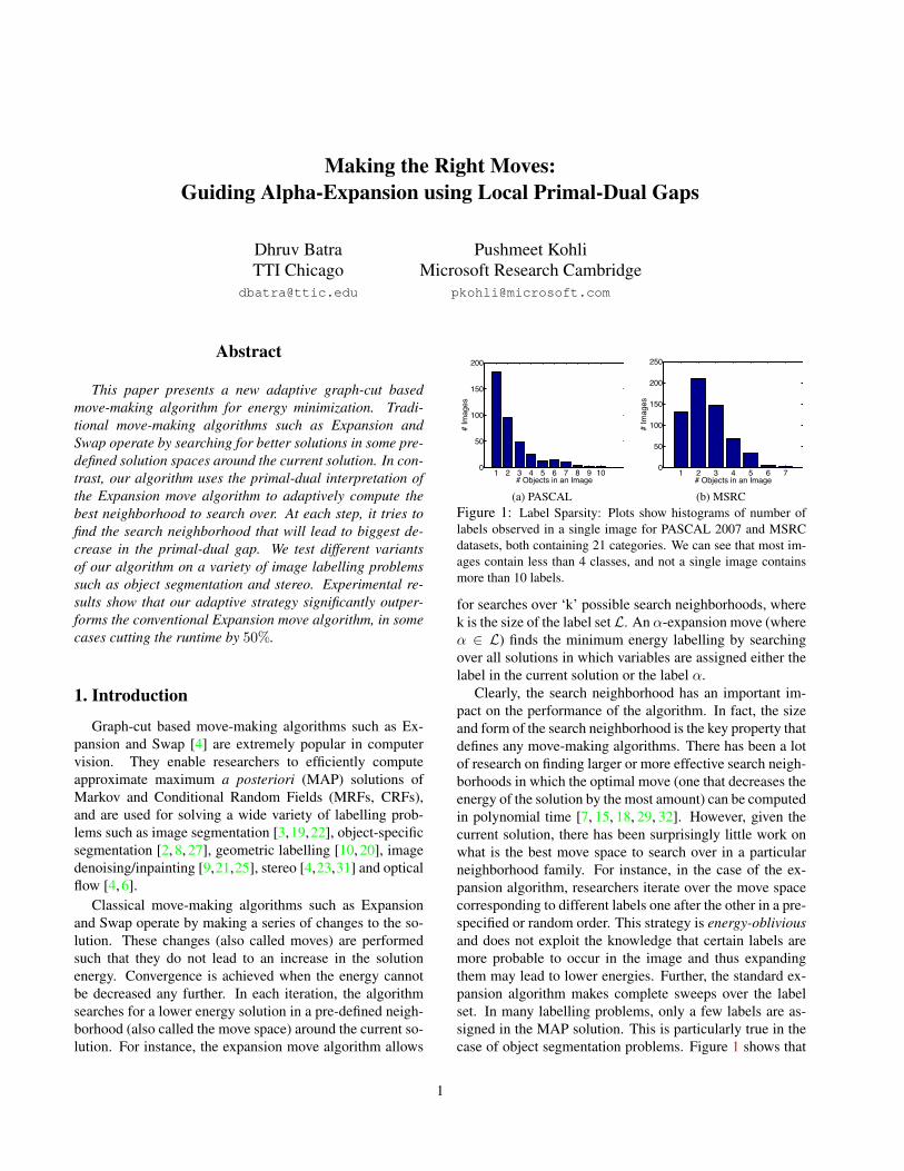
(b) MSRCFigure 1: Label Sparsity: Plots show histograms of number oflabels observed in a single image for PASCAL 2007 and MSRCdatasets, both containing 21 categories. We can see that most im-ages contain less than 4 classes, and not a single image containsmore than 10 labels.

for searches over ‘k’ possible search neighborhoods, wherek is the size of the label setL. An α-expansion move (whereα ∈ L) finds the minimum energy labelling by searchingover all solutions in which variables are assigned either thelabel in the current solution or the label α.

Clearly, the search neighborhood has an important im-pact on the performance of the algorithm. In fact, the sizeand form of the search neighborhood is the key property thatdefines any move-making algorithms. There has been a lotof research on finding larger or more effective search neigh-borhoods in which the optimal move (one that decreases theenergy of the solution by the most amount) can be computedin polynomial time [7, 15, 18, 29, 32]. However, given thecurrent solution, there has been surprisingly little work onwhat is the best move space to search over in a particularneighborhood family. For instance, in the case of the ex-pansion algorithm, researchers iterate over the move spacecorresponding to different labels one after the other in a pre-specified or random order. This strategy is energy-obliviousand does not exploit the knowledge that certain labels aremore probable to occur in the image and thus expandingthem may lead to lower energies. Further, the standard ex-pansion algorithm makes complete sweeps over the labelset. In many labelling problems, only a few labels are as-signed in the MAP solution. This is particularly true in thecase of object segmentation problems. Figure 1 shows that

1

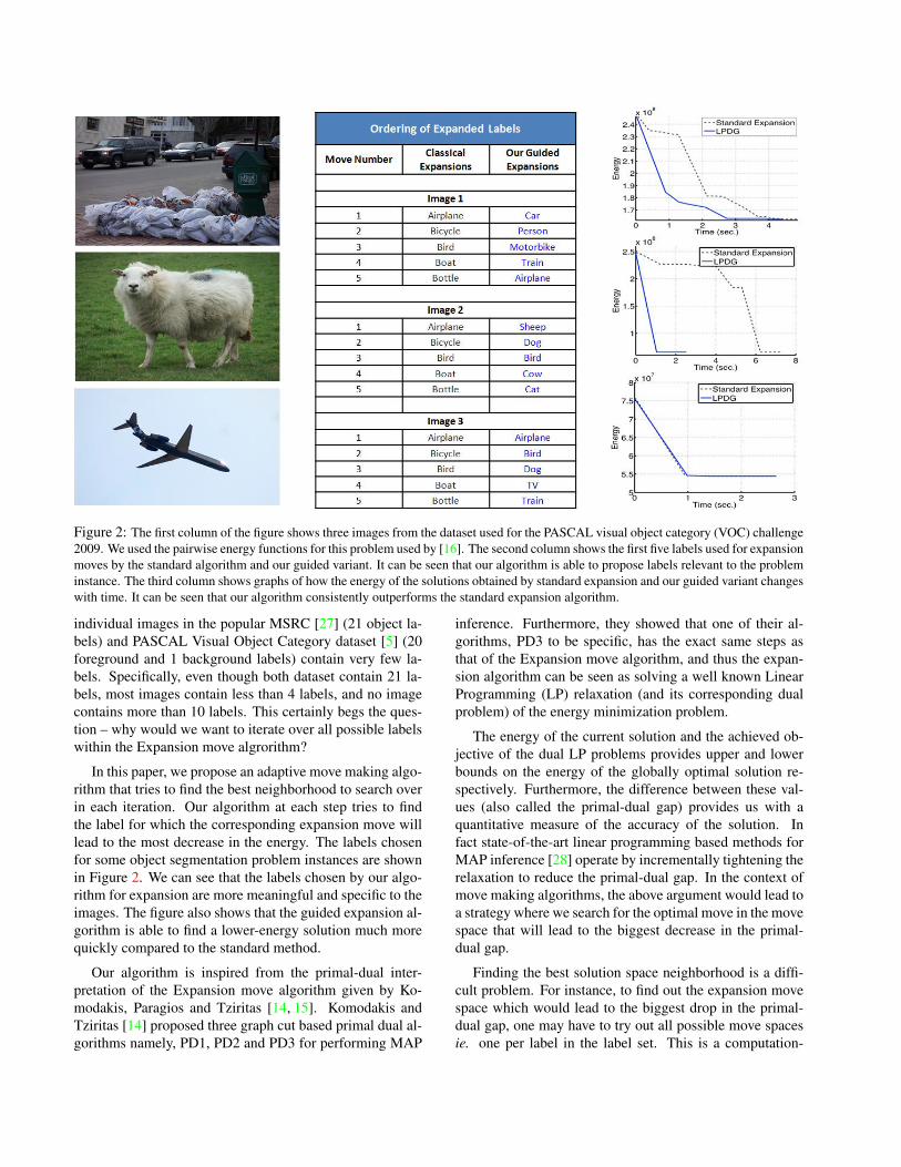
Figure 2: The first column of the figure shows three images from the dataset used for the PASCAL visual object category (VOC) challenge2009. We used the pairwise energy functions for this problem used by [16]. The second column shows the first five labels used for expansionmoves by the standard algorithm and our guided variant. It can be seen that our algorithm is able to propose labels relevant to the probleminstance. The third column shows graphs of how the energy of the solutions obtained by standard expansion and our guided variant changeswith time. It can be seen that our algorithm consistently outperforms the standard expansion algorithm.

individual images in the popular MSRC [27] (21 object la-bels) and PASCAL Visual Object Category dataset [5] (20foreground and 1 background labels) contain very few la-bels. Specifically, even though both dataset contain 21 la-bels, most images contain less than 4 labels, and no imagecontains more than 10 labels. This certainly begs the ques-tion – why would we want to iterate over all possible labelswithin the Expansion move algrorithm?

In this paper, we propose an adaptive move making algo-rithm that tries to find the best neighborhood to search overin each iteration. Our algorithm at each step tries to findthe label for which the corresponding expansion move willlead to the most decrease in the energy. The labels chosenfor some object segmentation problem instances are shownin Figure 2. We can see that the labels chosen by our algo-rithm for expansion are more meaningful and specific to theimages. The figure also shows that the guided expansion al-gorithm is able to find a lower-energy solution much morequickly compared to the standard method.

Our algorithm is inspired from the primal-dual inter-pretation of the Expansion move algorithm given by Ko-modakis, Paragios and Tziritas [14, 15]. Komodakis andTziritas [14] proposed three graph cut based primal dual al-gorithms namely, PD1, PD2 and PD3 for performing MAP

inference. Furthermore, they showed that one of their al-gorithms, PD3 to be specific, has the exact same steps asthat of the Expansion move algorithm, and thus the expan-sion algorithm can be seen as solving a well known LinearProgramming (LP) relaxation (and its corresponding dualproblem) of the energy minimization problem.

The energy of the current solution and the achieved ob-jective of the dual LP problems provides upper and lowerbounds on the energy of the globally optimal solution re-spectively. Furthermore, the difference between these val-ues (also called the primal-dual gap) provides us with aquantitative measure of the accuracy of the solution. Infact state-of-the-art linear programming based methods forMAP inference [28] operate by incrementally tightening therelaxation to reduce the primal-dual gap. In the context ofmove making algorithms, the above argument would lead toa strategy where we search for the optimal move in the movespace that will lead to the biggest decrease in the primal-dual gap.

Finding the best solution space neighborhood is a diffi-cult problem. For instance, to find out the expansion movespace which would lead to the biggest drop in the primal-dual gap, one may have to try out all possible move spacesie. one per label in the label set. This is a computation-

ally expensive operation and would make the algorithm veryslow. The key observation of this paper is that a good ap-proximation to the relative drop in the primal-dual gap cor-responding to different expansion move spaces can be foundusing the primal and dual variables of the LP formulation ofthe problem. This approach is extremely efficient and runsin linear time in the number of variables and labels. Wetest the efficacy of our method on a number of image la-belling problems. The experimental results show that ouradaptive method significantly outperforms the widely usedtraditional Expansion move algorithm.

An outline of the paper follows. Section 2 describes thework most closely related to ours. Section 3 provides thenotation and explains the primal-dual formulation of the en-ergy minimization problem. Section 4 explains our meth-ods for finding good expansion moves. The details of thelabelling problems used for testing the algorithm, and theexperimental results are given in Section 5. Section 6 con-cludes the paper by summarizing the main ideas and dis-cussing directions for future work.

2. Related WorkThe last few years have seen the proposal of a number of

sophisticated methods to improve the efficiency of move-making algorithms such as Expansion [1, 15, 18, 32]. Thesemethods can be divided into two broad categories: energy-oblivious and energy-aware.

Energy-oblivious methods do not use the knowledge ofthe energy function to reduce computation time. The FAST-PD algorithm proposed by Komodakis et al. [15] and a re-lated but simpler algorithm proposed by Alahari et al. [1]are two such methods. They use results of initial iterationsof the expansion algorithm to make subsequent iterationsfaster, and are inspired from the the dynamic graph cuts al-gorithm proposed by Kohli and Torr [13]. Another exampleis the fusion move algorithm which was independently pro-posed by Lempitsky et al. [18] and Woodford et al. [32].This algorithm uses proposal solutions of the labeling prob-lem obtained from different methods for defining the movespace for the move making algorithm.

Our algorithm belongs to the class of energy-aware tech-niques which use the energy function to guide the search.The only other method which belongs to this class isthe gradient-descent fusion-move algorithm proposed byIshikawa [11]. This method tries to find the most promis-ing move-space to search over by using the gradient of theenergy function.

3. Notation and PreliminariesWe start by providing the notation used in the

manuscript. For any positive integer n, let [n] be shorthandfor the set {1, 2, . . . , n}. We consider a set of discrete ran-

dom variables X = {x1, x2, . . . , xn}, each taking value ina finite label set Xi = {l1, l2, ..., lk}. For simplicity of no-tation, we may assume Xi = L ∀i. Let G = (V, E) be agraph defined over these variables, i.e. V = [n], E ⊆

([n]2

).

The goal of MAP inference is to find the labelling x of thevariables which minimize a real-valued energy function as-sociated with this graph:

minX

E(x) = minX

∑i∈V

θi(xi) +∑

(i,j)∈E

θij(xi, xj)

,

(1)where θi(·), θij(·, ·) denote node and edge energies.

3.1. The Expansion Move Algorithm

The expansion algorithm starts with an initial solutionand proceeds by making a series of changes which lead tosolutions having lower energy. An expansion move over alabel α ∈ L allows any random variable to either retain itscurrent label or take label α. One sweep of the algorithminvolves making moves for all α ∈ L in some order succes-sively.

Following the notation of Kohli et al. [12], we uset ={ti | ∀i ∈ V} to denote a vector of binary variables thatencodes an expansion move. The binary variable ti indi-cates whether variable xi retains its current label or takesthe label α. A transformation function T (x, t) takes thecurrent labelling x and a move t and returns the new la-belling x which has been induced by the move. The energyof a move t (denoted by Em(t)) is defined as the energy ofthe labelling x it induces, i.e. Em(t) = E(T (x, t)). Theoptimal move is defined as t∗ = argmintE(T (x, t)).

The transformation function Tα() for an α-expansionmove transforms the label of a random variable xi as

Tα(xi, ti) =

{xi if ti = 0α if ti = 1.

(2)

The optimal α-expansion move can be computed in poly-nomial time if the pairwise energy parameters θij define ametric. The energy parameter θij is said to be a metric if itsatisfies the conditions

θij(a, b) = 0 ⇐⇒ a = b, (3)θij(a, b) = θij(b, a) ≥ 0 (4)θij(a, c) ≤ θij(a, b) + θij(b, c) (5)

for all labels a, b and c in L.In this work, we do not assume the pairwise energies

to be metrics. We only require: θij(a, a) = 0, ∀a andθij(a, b) ≥ 0.

3.2. The Integer Program Formulation

MAP inference is typically set up as an integer pro-gramming problem over the boolean variables. Let

µi(s), µij(s, t) ∈ {0, 1} be indicator variables, such that{µi(s) = 1 ⇔ xi = s}, and {µij(s, t) = 1 ⇔ xi =s, xj = t}. Moreover, let µi = {µi(s) | s ∈ Xi},θi ={θi(s) | s ∈ Xi} be vectors of indicator-variables and en-ergies for node i. Let µij and θij be defined analogously.Using this notation, the MAP inference integer program canbe written as:

minµi,µij

∑i∈V

θi · µi +∑

(i,j)∈E

θij · µij (6)

s.t.∑s∈Xi

µi(s) = 1 ∀i ∈ V∑s∈Xi

µij(s, t) = µj(t) ∀(i, j), (j, i) ∈ E

µi(s), µij(s, t) ∈ {0, 1}

3.3. The primal-dual formulation

Problem (6) is known to be NP-hard in general [26].The standard LP relaxation of this problem, also known asSchlesingers bound [24, 30], is given by:

minµi,µij

∑i∈V

θi · µi +∑

(i,j)∈E

θij · µij (7)

s.t.∑s∈Xi

µi(s) = 1 ∀i ∈ V∑s∈Xi

µij(s, t) = µj(t) ∀(i, j), (j, i) ∈ E

µi(s), µij(s, t) ≥ 0

3.4. The Primal-dual Interpretation of Expansion

Komodakis et al. [14, 15] gave a primal-dual interpreta-tion of α-expansion. The LP-dual of (7) that they chose towork with was:

maxhi,yij(t)

∑i∈V

hi (8)

s.t. hi ≤ hi(s) ∀i ∈ V, syij(t) + yji(s) ≤ θij(s, t) ∀(i, j) ∈ E , s, thi, yij(t) ∈ R,

where hi(s).= θi(s) +

∑j∈N (i) yji(s).

One of the benefits of an primal-dual formulation is thatevery feasible dual solution provides a lower-bound on theMAP value, i.e.:

E(x) ≥ E(x∗) ≥∑i∈V

hi (9)

Moreover, for any primal labelling X p, the quantity primal-dual gap –

∑i∈V θi(x

pi )+

∑(i,j)∈E θij(x

pi , x

pj )−

∑i∈V hi –

gives an estimate of the tightness of the relaxation. Specifi-cally, a pair of primal-dual solutions (xp, {hi, yij(t)}) is an

θij(·, ·)

hi(xpi )

hi(α)

hj(α)

hj(xpj )

+δ−δ

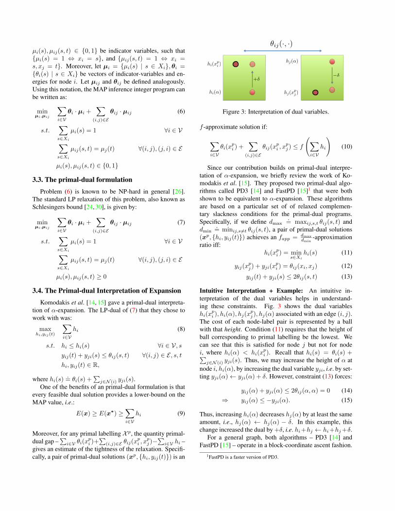
Figure 3: Interpretation of dual variables.

f -approximate solution if:

∑i∈V

θi(xpi ) +

∑(i,j)∈E

θij(xpi , x

pj ) ≤ f

(∑i∈V

hi

)(10)

Since our contribution builds on primal-dual interpre-tation of α-expansion, we briefly review the work of Ko-modakis et al. [15]. They proposed two primal-dual algo-rithms called PD3 [14] and FastPD [15]1 that were bothshown to be equivalent to α-expansion. These algorithmsare based on a particular set of of relaxed complemen-tary slackness conditions for the primal-dual programs.Specifically, if we define dmax

.= maxij,s,t θij(s, t) and

dmin.= minij,s 6=t θij(s, t), a pair of primal-dual solutions

(xp, {hi, yij(t)}) achieves an fapp = dmax

dmin-approximation

ratio iff:hi(x

pi ) = min

s∈Xi

hi(s) (11)

yij(xpj ) + yji(x

pi ) = θij(xi, xj) (12)

yij(t) + yji(s) ≤ 2θij(s, t) (13)

Intuitive Interpretation + Example: An intuitive in-terpretation of the dual variables helps in understand-ing these constraints. Fig. 3 shows the dual variableshi(x

pi ), hi(α), hj(x

pj ), hj(α) associated with an edge (i, j).

The cost of each node-label pair is represented by a ballwith that height. Condition (11) requires that the height ofball corresponding to primal labelling be the lowest. Wecan see that this is satisfied for node j but not for nodei, where hi(α) < hi(x

pi ). Recall that hi(s) = θi(s) +∑

j∈N (i) yji(s). Thus, we may increase the height of α atnode i, hi(α), by increasing the dual variable yji, i.e. by set-ting yji(α)← yji(α) + δ. However, constraint (13) forces:

yij(α) + yji(α) ≤ 2θij(α, α) = 0 (14)⇒ yij(α) ≤ −yji(α). (15)

Thus, increasing hi(α) decreases hj(α) by at least the sameamount, i.e., hj(α) ← hj(α) − δ. In this example, thischange increased the dual by +δ, i.e. hi+hj ← hi+hj+δ.

For a general graph, both algorithms – PD3 [14] andFastPD [15] – operate in a block-coordinate ascent fashion.

1FastPD is a faster version of PD3.

They loop over labels in a pre-determined order and at eachstep optimize all dual-variables corresponding to a label α,while holding all other dual variables fixed.

• Loop on label α ∈ L:

–α-expansion: Update {hi, hi(α), yij(α), yji(α)}

In both algorithms, conditions (12), (13) are satisfied byconstruction, and the goal of these block-updates is to makeprogress on condition (11), i.e. to extract a primal labellingthat has the minimal height at all nodes.

4. Adaptive Primal-Dual Expansion MovesIn this paper we focus on the step 1, i.e. how to enumer-

ate over the labels for primal-dual expansion moves. Typ-ical choices are to loop over labels one after the other in apre-specified or random order. This is exactly the schemethat FastPD follows. We follow an energy-aware strategythat uses the primal and dual variables to make adaptive ex-pansion moves. Specifically, we present a label proposalheuristic that sorts labels according to a scoring functionthat quantifies how helpful a label will be for α-expansion.Our label scoring function is derived from complementaryslackness condition (11).

4.1. Local-Primal Dual Gap

We first define a quantity we call Local Primal-Dual Gap(LPDG) for every label and variable. LPDG is formallydefines as:

l(i | α) = hi(xpi )− hi(α). (16)

Using the ball analogy of dual variables from Figure 3again, LPDG can be seen as the height difference betweenthe balls at node i corresponding to the primal labelling xpiand the label α. Positive values of LPDG indicate viola-tions of complementary slackness, and we can say that dualvariable hi(α) is in deficit by an amount of l(i | α). Neg-ative values of LPDG indicate that complementary slack-ness is satisfied and that dual variable hi(α) is in surplus byamount l(i | α). A dual variable in deficit hi(α) needs tobe “fixed” by the algorithm and a dual variable in surplushj(α) can help this process by via the message-variablesyij(α), yji(α).

Comparing (11) and (16), we can see that intuitivelyLPDG quantifies the amount of violation in complementaryslackness conditions, and also attributes violations to spe-cific nodes and labels. More specifically, we can state thefollowing property of LPDG:

Proposition 1 Slackness: If LPDG for all nodes is non-positive, i.e. l(i | α) ≤ 0, ∀i ∈ V, α, then complementaryslackness conditions hold and we have achieved an fapp-approximate solution.

Algorithm 1 LPDG-Sweep1: for t = 0, 1, . . . do2: Compute LPDG-based label scores ω(·) ∈

{ω1(·), ω2(·), ω3(·)}.3: Sort label scores: {α1, . . . , αk} = sort(ω(·))4: for i = 1, . . . , k do5: αi-expansion: Update variables:

{hi, hi(α), yij(α), yji(α)}6: end for7: end for

4.2. LPDG-based Label Scoring Functions

LPDG gives us an appropriate language to describe ourgoals for label scoring. In order to get the highest dropin primal-dual gap, we need to pick a label α that hasthe deficit. However, we also need to make sure there isenough surplus so that we may actually make an improve-ment. Keeping this in mind, we propose the following threelabel scoring functions:

• LPDG-crisp:ω1(α) =

∑i∈V sign

(l(i | α)

),

where sign(y) ={

1 y ≥ 00 else (17)

• LPDG-deficit:ω2(α) =

∑i∈V [[ l(i | α) ]]+

where [[ y ]] =

{y y ≥ 00 else (18)

• LPDG-tradeoff:ω3(α) =

∑i∈V

∣∣l(i | α)∣∣LPDG-crisp ignores the actual LPDG values and sim-

ply counts the number of nodes in deficit. LPDG-deficit onthe other hand also incorporates the how much these nodesare in deficit. Finally, LPDG-tradeoff incorporates both theamount of deficit and the surplus over all nodes.

Finally, we propose the following two adaptive primal-dual expansion algorithms: 1) LPDG-Sweep, shown inAlg 1 that uses an LPDG scoring function based permu-tation of labels to perform alpha-expansion in each sweep,and 2) LPDG-Partial-Sweep, show in Alg. 2, that performspartial sweeps where LPDG-based reordering of labels isperformed after each alpha-expansion.

The standard expansion algorithm goes through all la-bels in one iteration, and thus has a linear runtime complex-ity in the number of labels in the problem. This had madeit inefficient on problems with very large label sets. Ourpartial-sweep scheme based on LPDG scores is not boundto the linear complexity and only expands labels which arerelevant to the problem instance.

0 1 2 3 4x 107

0

2

4

6

8

10x 104

LPDG crisp

Dec

reas

e in

Prim

al

(a) LPDG-crisp.

0 1 2 3 4x 107

0

1

2

3

4x 107

LPDG deficit

Dec

reas

e in

Prim

al(b) LPDG-deficit.

0 1 2 3 4x 107

0

1

2

3

4

5x 107

LPDG tradeoff

Dec

reas

e in

Prim

al

(c) LPDG-tradeoff.

1 2 3 4 50.2

0

0.2

0.4

0.6

0.8

1

1.2

# Expansions

Cor

rela

tion

Coe

ffien

t

LPDG crispLPDG deficitLPDG tradeoff

(d) Correlation Coefficients.

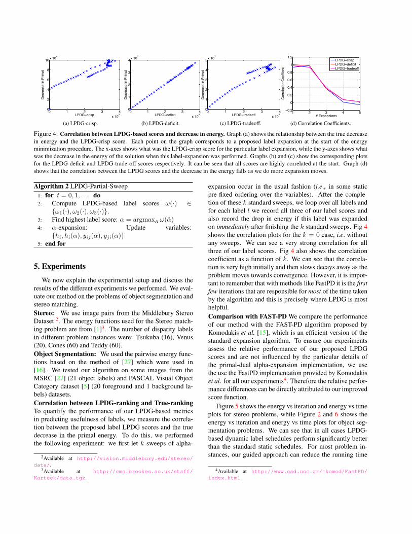
Figure 4: Correlation between LPDG-based scores and decrease in energy. Graph (a) shows the relationship between the true decreasein energy and the LPDG-crisp score. Each point on the graph corresponds to a proposed label expansion at the start of the energyminimization procedure. The x-axes shows what was the LPDG-crisp score for the particular label expansion, while the y-axes shows whatwas the decrease in the energy of the solution when this label-expansion was performed. Graphs (b) and (c) show the corresponding plotsfor the LPDG-deficit and LPDG-trade-off scores respectively. It can be seen that all scores are highly correlated at the start. Graph (d)shows that the correlation between the LPDG scores and the decrease in the energy falls as we do more expansion moves.

Algorithm 2 LPDG-Partial-Sweep1: for t = 0, 1, . . . do2: Compute LPDG-based label scores ω(·) ∈

{ω1(·), ω2(·), ω3(·)}.3: Find highest label score: α = argmaxα ω(α)4: α-expansion: Update variables:

{hi, hi(α), yij(α), yji(α)}5: end for

5. Experiments

We now explain the experimental setup and discuss theresults of the different experiments we performed. We eval-uate our method on the problems of object segmentation andstereo matching.Stereo: We use image pairs from the Middlebury StereoDataset 2. The energy functions used for the Stereo match-ing problem are from [1]3. The number of disparity labelsin different problem instances were: Tsukuba (16), Venus(20), Cones (60) and Teddy (60).Object Segmentation: We used the pairwise energy func-tions based on the method of [27] which were used in[16]. We tested our algorithm on some images from theMSRC [27] (21 object labels) and PASCAL Visual ObjectCategory dataset [5] (20 foreground and 1 background la-bels) datasets.Correlation between LPDG-ranking and True-rankingTo quantify the performance of our LPDG-based metricsin predicting usefulness of labels, we measure the correla-tion between the proposed label LPDG scores and the truedecrease in the primal energy. To do this, we performedthe following experiment: we first let k sweeps of alpha-

2Available at http://vision.middlebury.edu/stereo/data/.

3Available at http://cms.brookes.ac.uk/staff/Karteek/data.tgz.

expansion occur in the usual fashion (i.e., in some staticpre-fixed ordering over the variables). After the comple-tion of these k standard sweeps, we loop over all labels andfor each label l we record all three of our label scores andalso record the drop in energy if this label was expandedon immediately after finishing the k standard sweeps. Fig 4shows the correlation plots for the k = 0 case, i.e. withoutany sweeps. We can see a very strong correlation for allthree of our label scores. Fig 4 also shows the correlationcoefficient as a function of k. We can see that the correla-tion is very high initially and then slows decays away as theproblem moves towards convergence. However, it is impor-tant to remember that with methods like FastPD it is the firstfew iterations that are responsible for most of the time takenby the algorithm and this is precisely where LPDG is mosthelpful.Comparison with FAST-PD We compare the performanceof our method with the FAST-PD algorithm proposed byKomodakis et al. [15], which is an efficient version of thestandard expansion algorithm. To ensure our experimentsassess the relative performance of our proposed LPDGscores and are not influenced by the particular details ofthe primal-dual alpha-expansion implementation, we usethe use the FastPD implementation provided by Komodakiset al. for all our experiments4. Therefore the relative perfor-mance differences can be directly attributed to our improvedscore function.

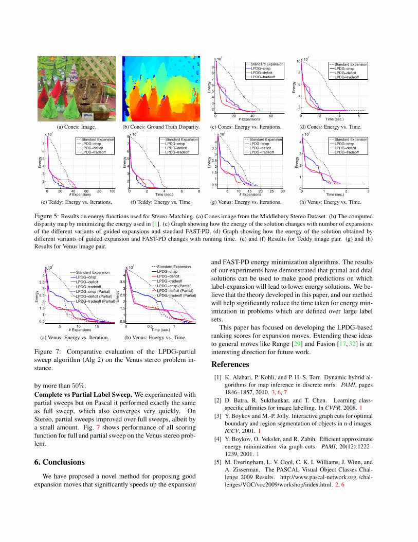
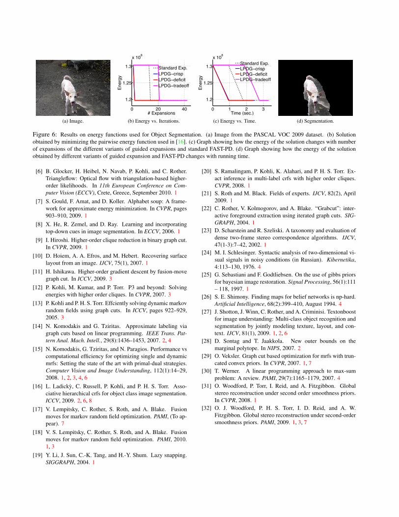
Figure 5 shows the energy vs iteration and energy vs timeplots for stereo problems, while Figure 2 and 6 shows theenergy vs iteration and energy vs time plots for object seg-mentation problems. We can see that in all cases LPDG-based dynamic label schedules perform significantly betterthan the standard static schedules. For most problem in-stances, our guided approach can reduce the running time

4Available at http://www.csd.uoc.gr/˜komod/FastPD/index.html.

(a) Cones: Image. (b) Cones: Ground Truth Disparity.

0 20 40 60

23456789

x 107

# Expansions

Ener

gy

Standard ExpansionLPDG crispLPDG deficitLPDG tradeoff

(c) Cones: Energy vs. Iterations.

0 2 4 6

2

4

6

8

10x 107

Time (sec.)

Ener

gy

Standard ExpansionLPDG crispLPDG deficitLPDG tradeoff

(d) Cones: Energy vs. Time.

0 20 40 60 80 100

2

3

4

5

6

7

x 107

# Expansions

Ener

gy

Standard ExpansionLPDG crispLPDG deficitLPDG tradeoff

(e) Teddy: Energy vs. Iterations.

0 2 4 6 81

2

3

4

5

6

7

8x 107

Time (sec.)

Ener

gy

Standard ExpansionLPDG crispLPDG deficitLPDG tradeoff

(f) Teddy: Energy vs. Time.

5 10 15 20 25 300.5

11.5

22.5

33.5

4

x 107

# Expansions

Ener

gy

Standard ExpansionLPDG crispLPDG deficitLPDG tradeoff

(g) Venus: Energy vs. Iterations.

0 1 2 30

1

2

3

4

x 107

Time (sec.)

Ener

gy

Standard ExpansionLPDG crispLPDG deficitLPDG tradeoff

(h) Venus: Energy vs. Time.

Figure 5: Results on energy functions used for Stereo-Matching. (a) Cones image from the Middlebury Stereo Dataset. (b) The computeddisparity map by minimizing the energy used in [1]. (c) Graph showing how the energy of the solution changes with number of expansionsof the different variants of guided expansions and standard FAST-PD. (d) Graph showing how the energy of the solution obtained bydifferent variants of guided expansion and FAST-PD changes with running time. (e) and (f) Results for Teddy image pair. (g) and (h)Results for Venus image pair.

5 10 150.5

11.5

22.5

33.5

4

x 107

# Expansions

Ener

gy

Standard ExpansionLPDG crispLPDG deficitLPDG tradeoffLPDG crisp (Partial)LPDG deficit (Partial)LPDG tradeoff (Partial)

(a) Venus: Energy vs. Iteration.

0 0.5 10.5

11.5

22.5

33.5

4

x 107

Time (sec.)

Ener

gy

Standard ExpansionLPDG crispLPDG deficitLPDG tradeoffLPDG crisp (Partial)LPDG deficit (Partial)LPDG tradeoff (Partial)

(b) Venus: Energy vs. Time.

Figure 7: Comparative evaluation of the LPDG-partialsweep algorithm (Alg 2) on the Venus stereo problem in-stance.

by more than 50%.Complete vs Partial Label Sweep. We experimented withpartial sweeps but on Pascal it performed exactly the sameas full sweep, which also converges very quickly. OnStereo, partial sweeps improved over full sweeps, albeit bya small amount. Fig. 7 shows performance of all scoringfunction for full and partial sweep on the Venus stereo prob-lem.

6. Conclusions

We have proposed a novel method for proposing goodexpansion moves that significantly speeds up the expansion

and FAST-PD energy minimization algorithms. The resultsof our experiments have demonstrated that primal and dualsolutions can be used to make good predictions on whichlabel-expansion will lead to lower energy solutions. We be-lieve that the theory developed in this paper, and our methodwill help significantly reduce the time taken for energy min-imization in problems which are defined over large labelsets.

This paper has focused on developing the LPDG-basedranking scores for expansion moves. Extending these ideasto general moves like Range [29] and Fusion [17, 32] is aninteresting direction for future work.

References[1] K. Alahari, P. Kohli, and P. H. S. Torr. Dynamic hybrid al-

gorithms for map inference in discrete mrfs. PAMI, pages1846–1857, 2010. 3, 6, 7

[2] D. Batra, R. Sukthankar, and T. Chen. Learning class-specific affinities for image labelling. In CVPR, 2008. 1

[3] Y. Boykov and M.-P. Jolly. Interactive graph cuts for optimalboundary and region segmentation of objects in n-d images.ICCV, 2001. 1

[4] Y. Boykov, O. Veksler, and R. Zabih. Efficient approximateenergy minimization via graph cuts. PAMI, 20(12):1222–1239, 2001. 1

[5] M. Everingham, L. V. Gool, C. K. I. Williams, J. Winn, andA. Zisserman. The PASCAL Visual Object Classes Chal-lenge 2009 Results. http://www.pascal-network.org /chal-lenges/VOC/voc2009/workshop/index.html. 2, 6

(a) Image.

0 20 40

1.2

1.25

1.3

x 108

# ExpansionsEn

ergy

Standard Exp.LPDG crispLPDG deficitLPDG tradeoff

(b) Energy vs. Iterations.

0 1 2 3

1.2

1.25

1.3

x 108

Time (sec.)

Ener

gy

Standard Exp.LPDG crispLPDG deficitLPDG tradeoff

(c) Energy vs. Time. (d) Segmentation.

Figure 6: Results on energy functions used for Object Segmentation. (a) Image from the PASCAL VOC 2009 dataset. (b) Solutionobtained by minimizing the pairwise energy function used in [16]. (c) Graph showing how the energy of the solution changes with numberof expansions of the different variants of guided expansions and standard FAST-PD. (d) Graph showing how the energy of the solutionobtained by different variants of guided expansion and FAST-PD changes with running time.

[6] B. Glocker, H. Heibel, N. Navab, P. Kohli, and C. Rother.Triangleflow: Optical flow with triangulation-based higher-order likelihoods. In 11th European Conference on Com-puter Vision (ECCV), Crete, Greece, September 2010. 1

[7] S. Gould, F. Amat, and D. Koller. Alphabet soup: A frame-work for approximate energy minimization. In CVPR, pages903–910, 2009. 1

[8] X. He, R. Zemel, and D. Ray. Learning and incorporatingtop-down cues in image segmentation. In ECCV, 2006. 1

[9] I. Hiroshi. Higher-order clique reduction in binary graph cut.In CVPR, 2009. 1

[10] D. Hoiem, A. A. Efros, and M. Hebert. Recovering surfacelayout from an image. IJCV, 75(1), 2007. 1

[11] H. Ishikawa. Higher-order gradient descent by fusion-movegraph cut. In ICCV, 2009. 3

[12] P. Kohli, M. Kumar, and P. Torr. P3 and beyond: Solvingenergies with higher order cliques. In CVPR, 2007. 3

[13] P. Kohli and P. H. S. Torr. Effciently solving dynamic markovrandom fields using graph cuts. In ICCV, pages 922–929,2005. 3

[14] N. Komodakis and G. Tziritas. Approximate labeling viagraph cuts based on linear programming. IEEE Trans. Pat-tern Anal. Mach. Intell., 29(8):1436–1453, 2007. 2, 4

[15] N. Komodakis, G. Tziritas, and N. Paragios. Performance vscomputational efficiency for optimizing single and dynamicmrfs: Setting the state of the art with primal-dual strategies.Computer Vision and Image Understanding, 112(1):14–29,2008. 1, 2, 3, 4, 6

[16] L. Ladicky, C. Russell, P. Kohli, and P. H. S. Torr. Asso-ciative hierarchical crfs for object class image segmentation.ICCV, 2009. 2, 6, 8

[17] V. Lempitsky, C. Rother, S. Roth, and A. Blake. Fusionmoves for markov random field optimization. PAMI, (To ap-pear). 7

[18] V. S. Lempitsky, C. Rother, S. Roth, and A. Blake. Fusionmoves for markov random field optimization. PAMI, 2010.1, 3

[19] Y. Li, J. Sun, C.-K. Tang, and H.-Y. Shum. Lazy snapping.SIGGRAPH, 2004. 1

[20] S. Ramalingam, P. Kohli, K. Alahari, and P. H. S. Torr. Ex-act inference in multi-label crfs with higher order cliques.CVPR, 2008. 1

[21] S. Roth and M. Black. Fields of experts. IJCV, 82(2), April2009. 1

[22] C. Rother, V. Kolmogorov, and A. Blake. “Grabcut”: inter-active foreground extraction using iterated graph cuts. SIG-GRAPH, 2004. 1

[23] D. Scharstein and R. Szeliski. A taxonomy and evaluation ofdense two-frame stereo correspondence algorithms. IJCV,47(1-3):7–42, 2002. 1

[24] M. I. Schlesinger. Syntactic analysis of two-dimensional vi-sual signals in noisy conditions (in Russian). Kibernetika,4:113–130, 1976. 4

[25] G. Sebastiani and F. Godtliebsen. On the use of gibbs priorsfor bayesian image restoration. Signal Processing, 56(1):111– 118, 1997. 1

[26] S. E. Shimony. Finding maps for belief networks is np-hard.Artificial Intelligence, 68(2):399–410, August 1994. 4

[27] J. Shotton, J. Winn, C. Rother, and A. Criminisi. Textonboostfor image understanding: Multi-class object recognition andsegmentation by jointly modeling texture, layout, and con-text. IJCV, 81(1), 2009. 1, 2, 6

[28] D. Sontag and T. Jaakkola. New outer bounds on themarginal polytope. In NIPS, 2007. 2

[29] O. Veksler. Graph cut based optimization for mrfs with trun-cated convex priors. In CVPR, 2007. 1, 7

[30] T. Werner. A linear programming approach to max-sumproblem: A review. PAMI, 29(7):1165–1179, 2007. 4

[31] O. Woodford, P. Torr, I. Reid, and A. Fitzgibbon. Globalstereo reconstruction under second order smoothness priors.In CVPR, 2008. 1

[32] O. J. Woodford, P. H. S. Torr, I. D. Reid, and A. W.Fitzgibbon. Global stereo reconstruction under second-ordersmoothness priors. PAMI, 2009. 1, 3, 7