1

Making friends with your neighbors? Agglomeration and tacit collusion in the lodging industry∗

Li Gan† and Manuel A. Hernandez‡

October 31, 2011

Abstract

Agglomeration is a location pattern frequently observed in service industries such as

hotels. This paper empirically examines whether agglomeration facilitates tacit collusion in

the lodging industry using a quarterly dataset of hotels that operated in rural areas across

Texas between 2003 and 2005. We jointly model a price and occupancy rate equation

under a switching regression model to endogenously identify a collusive and non-collusive

regime. The estimation results indicate that clustered hotels have a higher probability of

being in the potential collusive regime than isolated properties in the same town. The

identification of a collusive regime is also consistent with other factors considered to affect

the sustainability of tacit collusion like cluster size, seasonality and firm size, and the

results are robust to alternative cluster definitions.

Key Words: Collusion, Agglomeration, Lodging Industry, Switching regression model JEL Code: L13, L4, C3

∗ We thank the valuable comments of Jimmy Chan, Brian Viard, Steven Wiggins, and seminar participants at Texas A&M University, annual International Industrial Organization Conference, and the European Economic Association, Southern Economic Association, and the Allied Social Science Association annual meetings. We would also like to thank Philippe Aghion and two anonymous referees for their many helpful comments. † Department of Economics, Texas A&M University, and NBER. email: gan@econmail.tamu.edu. ‡ Markets, Trade, and Institutions Division, International Food Policy Research Institute (IFPRI), email: m.a.hernandez@cgiar.org.

2

1 Introduction

Agglomeration is a location pattern frequently observed in service industries such as the

lodging industry. A common assumption is that hotels locate close to one another to

enjoy of agglomeration effects. Fischer and Harrington (1996), for example, indicate that

in industries where products are heterogeneous and need personal inspection,

agglomeration results in a heightened demand. By spatially concentrating, sellers reduce

consumer’s search costs and attract more customers as a group relative to what they could

all attract individually.1 Helsley and Strange (1990) add that when firms are clustered,

they help consumers to better evaluate their options. In the case of the lodging industry,

Chung and Kalnins (2001) argue that agglomeration effects should be higher among

hotels located in rural areas since most of them are overnight destinations in between

days of travel, so a cluster of hotels may signal safety in an isolated area and/or indicate

the availability of additional services. Other studies that have analyzed agglomeration

effects in the hotel industry include Baum and Haveman (1997) and Kalnins and Chung

(2004). However, not much has been said about the possibility that agglomeration may

also facilitate the tacit coordination of prices and quantities among hotels located next to

each other. There is more anecdotal than empirical evidence on this matter.2

This paper seeks to empirically examine whether agglomeration facilitates tacit

collusion in the hotel industry. As revealed by Kalnins (2006), the exchange of price and

occupancy information among hotels appears to be very common in the industry (e.g. the

1 See also Stahl (1982) and Wolinsky (1983).

2 See Kalnins (2006) for some related examples.

3

practice of “call-arounds”). But agglomeration can provide further opportunities for

frequent interaction and exchange of information among hotel managers, and can also

facilitate the sustainability of a tacit collusive agreement (if any) by reducing monitoring

costs and increasing market transparency.3 On-site inspections, if necessary, of rates and

vacancy status are less costly among clustered hotels than among hotels located farther

apart, making it easier and faster to detect deviations from any potential tacit agreement.

For example, lobby visits by employees and observing the parking lot are less costly

among hotels located close to one another, and can provide some information about the

volume of check-ins. Several hotels in rural areas, particularly small-sized hotels of low

quality, also maintain the practice of posting signs with prices and/or “no vacancy” signs,

which further facilitates the monitoring between nearby hotels.4 We examine, then,

whether agglomeration facilitates a tacit coordination of prices and occupancy rates. To

our knowledge, this is the first empirical study to formally test this hypothesis.

The data used for the analysis is a quarterly data set of lodging properties that

operated in Non Metropolitan Statistical Areas (Non MSA) across Texas between 2003

and 2005. Using the physical address of each lodging property in the data set, we are able

to determine whether a hotel is clustered and the number of nearby competitors faced by

3 Our interviews with a couple of managers from hotels located close to one another confirm that they exchange information more frequently between them (usually more than once a day) than with managers from hotels farther apart, and adjust their rates accordingly. They call each other regularly, make personal visits or get together for formal or informal meetings, beside hospitality forums. Some managers also admitted that they actually observe their competitors parking lots on a regular basis or ask their employees to visit the other hotels’ lobbies or even encourage them to make friends with the employees of neighboring hotels. 4 The nature of our data, described later, suggests that the cost of monitoring may be a function of the distance to competing hotels in our sample. The use of the Internet, for example, as an alternative to on-site inspection for monitoring is not generally applicable in our case. By the time we did a search on the Web to verify the existence of the hotels in our sample, several of the hotels, particularly small-sized independent hotels, did not keep a website or if they did, the website did not allow to make reservations. Making phone calls, instead, may not be a reliable source of information for monitoring if you do it on a regular basis under a tacit agreement.

4

each hotel within each town. Working with geographically isolated areas also enables us

to avoid any market overlapping issues and correctly identify the total number of

competitors within each market, as in Bresnahan and Reiss (1991) and Mazzeo (2002).

Collusive regimes differ from non-collusive ones in higher prices and lower

quantities. The literature using regime switching models to identify collusive regimes so

far has been only using difference in prices. Since this paper identifies a collusive regime

using differences in both price and quantity (occupancy rate), it exhibits more power in

detecting collusive regimes in the literature.

In this paper, a hotel in the sample may follow a particular regime or alternate

between regimes across time. In the potential collusive regime with tacit coordination

among firms, prices are expected to be higher and quantities (occupancy rates) to be

lower, as predicted by general oligopoly models where firms interact repeatedly and find

it profitable to tacitly cooperate under the threat of future punishment.5 Additionally,

prices (and occupancy rates) are expected to exhibit a lower dispersion during

successfully collusive periods.6 We then analyze if agglomeration increases the

probability of being in the potential collusive regime.

Several methods have been developed in the literature to detect collusive behavior

or cartels. Bajari and Ye (2003) argue that competitive bids in auctions should be

independent with each other conditional on observed characteristics. Abrantes-Metz et

al. (2006) suggest a screen test for collusion using changes in the coefficient of variation

of prices. In this paper, we follow the method developed in Porter (1983), Ellison (1994)

5 See Tirole (1988), Ivaldi et al. (2003). 6 Recent studies suggesting that prices are more stable under collusion include Athey, Bagwell and Sanchirico (2004), Connor (2005) and Abrantes-Metz et al. (2006). For a general discussion on different behavioral patterns under collusion, refer to Harrington (2005).

5

and Knittel and Stango (2003) of using regime switching models to endogenously

identify collusive and non-collusive regimes. Porter (1983) estimates a switching

regression model to classify prices into collusive and non-collusive regimes during the

Joint Executive Committee cartel on railroads in the late 19th century; Ellison (1994)

reexamines the experience of the railroad cartel using a Markov structure on the

transitions between collusive and non-collusive periods; Knittel and Stango (2003) use a

mixture density model to test whether nonbinding price ceilings may serve as focal points

for tacit collusion in the credit card market. In their papers, a higher price regime is

associated with collusive behavior.

Further, we examine whether our identification strategy is consistent with other

factors thought to affect the sustainability of tacit collusion, as in Knittel and Stango

(2003). In particular, the probability of engaging in tacit collusion is allowed to vary with

cluster size, seasonality and firm size.

The estimation results suggest that agglomeration facilitates tacit collusion.

Clustered hotels show a higher probability of being in the suspected collusive regime

than isolated properties in the same town. Similarly, our identification of a collusive

regime is consistent with other factors considered to affect the sustainability of tacit

collusion, and the results are robust to alternative cluster definitions. Moreover, all hotels

without a competitor in town (i.e. monopolists), whose behavior should be equivalent to

perfect collusion, are always predicted to fall in the potential collusive regime when

deriving binary regime predictions.

The reminder of the paper is organized as follows. Section 2 further discusses

how agglomeration can facilitate tacit collusion. Section 3 describes the data and certain

6

empirical regularities of the lodging industry in rural areas across Texas. The empirical

model is presented in Section 4. Section 5 reports the estimation results while Section 6

concludes.

2 Agglomeration and tacit collusion

This section briefly discusses the economics of tacit collusion and how agglomeration

can facilitate the sustainability of a cooperative agreement among clustered firms. It is

well established that tacit collusion can arise when firms interact repeatedly in the same

market (Tirole, 1988; Ivaldi et al., 2003). Firms can achieve higher profits by tacitly

agreeing to raise prices (and restrict quantity) above (below) the static Nash equilibrium

level. Since cheating or deviating from the collusive agreement increases current profits,

firms can only be deterred from deviating if they are penalized in the future. For example,

if a firm deviates from the collusive or cooperative outcome at a particular time period,

the other firms may respond by reverting to the non-cooperative outcome for a certain

number of subsequent periods (or forever). The collusive equilibrium condition or

incentive compatibility (IC) constraint requires, then, that the present value of foregone

future profits is greater than or equal to the current profits from deviating.

Consider N firms each producing a differentiated product and competing in prices

in an infinitely repeated game. All firms share the same unit cost of production. Let

Nip si ,...,1, = , be the price that maximizes firm i’s profits ( s

iπ ) in the static version of

the game. If firms agree to cooperate by charging si

ci pp > and obtaining profits c

iπ in

each period, then the IC constraint requires that,

7

ci

di

T

t

si

ci

t ππππδ −≥−∑=1

)( (1)

where )1,0(∈δ is the discount factor equal across firms, diπ are firm i’s profits when

deviating from the collusive agreement and choosing best-response price dip given all

other firms’ prices cip− , and T are the number of periods of reversion to the non-collusive

outcome. Note that si

ci

di πππ >> . From the condition above, it follows that the collusive

outcome is more likely to be an equilibrium the higher the discount factor δ or when T is

sufficiently high.

Agglomeration can facilitate the sustainability of a tacit collusive agreement

under the assumption that it provides additional opportunities for frequent interaction and

exchange of information among hotel managers. The exchange of price and occupancy

information is a regular practice in the industry, but managers in hotels located close to

one another seem to interact and exchange information more frequently amongst

themselves than with managers of other hotels in town. Agglomeration can also be

thought to facilitate tacit collusion under the assumption that it reduces monitoring costs

and increases market transparency. On-site inspections (if necessary) of rates and

vacancy status through lobby visits by employees or by observing parking lots can

provide some information about the volume of check-ins, and are less costly among

clustered hotels than among hotels located farther apart. Additionally, several hotels in

rural areas, especially small-sized properties of low quality, maintain the practice of

posting signs with prices and/or “no vacancy” signs, which further facilitates the

monitoring among hotels located close to one another.

8

This implies, then, that clustered hotels can detect and react faster to any potential

deviation from a tacit agreement among them, and adjust their rates accordingly. In terms

of the condition described in equation (1), a faster reaction and retaliation both limits the

potential profits from deviating or short term profits diπ , and results in a higher discount

factor δ , which increases the perceived cost of future retaliation (Ivaldi et al., 2003).

Intuitively, firms will find it easier to cooperate and sustain a tacit agreement when they

can react more quickly to a deviation by one of them.7

As noted above, in the analysis we also control for factors, other than

agglomeration, that can affect the sustainability of tacit collusion.8 These other factors

include number of competitors (cluster size), seasonality and firm size. We discuss later

how these other variables can make a collusive agreement easier or more difficult to

sustain. Next, we describe the data used for the study and some empirical regularities of

the hotel industry in rural areas across Texas.

3 Data

The main data source is the Texas Hotel Performance Factbook, published every quarter

by Source Strategies Inc. This is a unique data set that contains information on room

counts, average daily rates (ADR), and occupancy rates for all lodging properties in

7 It is worth mentioning that in this study we take geographic location as given. Friedman and Thisse (1991) have also shown that agglomeration is the only equilibrium outcome when collusion on price follows competition on location. Locating at the same point implies that the firms’ ability to punish one another for defection is maximized once the equilibrium locations are selected. The authors develop a spatial duopoly model in which firms simultaneously select their locations at the beginning of time (once and forever) and choose prices in each of a countable infinite succession of time periods. The critical assumption in their model is that firms have the ability, at the beginning of the game, to determine the set of price outcomes that are admissible in the subsequent repeated subgames. 8 For an extensive description of factors that may facilitate tacit collusion see Ivaldi et al. (2003).

9

Texas exceeding 18,000 dollars per quarter in gross revenues.9 The data set also provides

the hotel name and address, and indicates whether each property is affiliated to a “Top

50+” chain.10 Hotels are ordered by MSA/Non MSA, city/town and zip code.

In this study, we focus on lodging properties that operated in Non MSA (towns)

across the state between 2003 and 2005.11 A market is defined as all hotels in a given

town. Hotels can, then, be located downtown or along the town boundaries, including

highway exits. Working with towns in rural areas allows us to work with a comparable

and geographically isolated set of oligopoly markets, as shown in Figure A.1 in the

Appendix. The map indicates that the locations in our sample are generally small and

separated from one another.12 This also limits the extent of inter-market competition and

helps to correctly identify the number of competitors in each market, as in Bresnahan and

Reiss (1991) and Mazzeo (2002).13 We still control for physical distance to the next

closest location in our sample, provided that hotels adjacent to a highway exit in a

particular town may also compete to some extent for travelers with hotels at other exits in

the same highway but in a different town. 9 See Table A.1 for a more detailed description of these variables. According to SSI, properties below 18,000 dollars per quarter result in approximately 1.5% of the total state revenues being excluded from this database. To our knowledge, this is one of the few datasets that provide detailed financial information of each lodging property in a whole state. Smith Travel Research (STR), a leading private research firm in the lodging industry, gets full financial reports from hotels/motels accounting for 80% of the market but only publishes aggregate results. They also maintain a Lodging Census Database which does not include financial information. 10 The “Top 50+” chains are determined and tracked by Source Strategies Inc., and may vary across time. 11 The second semester of 2005 may be an atypical period because of the sudden increase in the demand for hotel rooms after Katrina and Rita. However, according to a list of hotels/motels that participated in the Federal Emergency Management Agency’s (FEMA) temporary housing program, provided by the same agency, most of the evacuees in Texas relocated in urban areas. In any case, we include time-period dummies in our estimates. 12 The average and minimum longitudinal (Euclidean) distance between locations (towns) is 266 and 16 miles, respectively. The whole list of locations, by region, is reported in Table A.2. 13 Bresnahan and Reiss (1991) study the relationship between the number of firms, market size and competition using a sample of 202 isolated local markets (county seats) in the western United States. Mazzeo (2002), in turn, analyzes the effect of market concentration and product differentiation on market outcomes using a cross section of 492 isolated motel markets located adjacent to small, rural exits along one of the 30 longest U.S. interstate highways.

10

Overall, we have an unbalanced panel of 9,148 observations corresponding to 845

hotels operating in 250 markets between the first quarter of 2003 and the fourth quarter of

2005.14 We also assigned a product type to each hotel, either low or high quality, based

on the quality ratings (“diamonds”) from the American Automobile Association’s (AAA)

online hotel directory (www.aaa-texas.com). Hotels are rated from one to four diamonds

in our sample, ranging from simple to upscale. Following Mazzeo (2002), we define low

quality as one diamond and high quality as two or more diamonds. For those “Top 50+”

chain-affiliated hotels not listed in the directory, we assigned the modal category of other

chain-affiliated members that were in fact rated. Since AAA has minimum quality

standards for inclusion of hotels in their directory, we assigned the lowest category for

independent properties and other minor chains not listed.

The data set was finally complemented with several market controls for cost and

demand conditions widely used in previous studies on the lodging industry (see Baum

and Haveman, 1997; Chung and Kalnins, 2001; Mazzeo, 2002; Kalnins and Chung,

2004). These variables include population, per capita personal income, number of gas

stations at each location, value of rural land per acre, weekly wage on leisure and

hospitality, distance to MSA, distance to the next closest location, and regional

dummies.15 Table A.3 describes the sources of information consulted to construct these

variables.

3.1 The Lodging Industry in Non MSA across Texas

14 The unbalanced panel results from the fact that the information for certain hotels and markets is not fully reported by SSI across all periods, and due to a small number of entries/exits in some markets. 15 Distance to MSA is measured as the mileage between the town and the nearest MSA; distance to the next closest location is physical distance to the next closest town in our sample.

11

Table 1 presents the distribution of markets by number of operating firms at each quarter

during the period 2003-2005.16 It follows that our sample basically consists of small

oligopolies. In four of every five markets observed, there are five or less hotels operating.

More specifically, 37% of the markets are monopolies, 18% are duopolies and another

26% have between three and five competitors.

With respect to the geographical location of hotels in a market relative to the other

competitors in town, we allocate each hotel to one of four possible location categories:

clustered, isolated with a cluster of hotels in town, monopolist, and isolated without any

cluster in town. A hotel is considered clustered if it has at least one competitor in a radius

of 0.2 miles. An isolated property with a cluster in town is a hotel with competitors in

town that are more than 0.2 miles from the hotel, but where at least two of these

competitors are within 0.2 miles from each other. A monopolist, in turn, is a hotel

without any competitors in town, while an isolated property with no cluster in town is a

hotel with competitors in town that are all more than 0.2 miles apart from each other.

Since the exact extent of a cluster is an empirical matter, we limit the cluster

radius to 0.2 miles and later compare our estimation results to those obtained under other

two alternative measures: 0.1 and 0.5 miles.17 These conservative measures are also in

line with the idea that for agglomeration to facilitate the sustainability of a tacit collusive

agreement, hotels should be located sufficiently close to each other to decrease

monitoring costs and increase market transparency, and for managers to interact and

16 Considering that we have data for 12 quarters, each market can be observed up to 12 times. 17 This empirical issue is similar to the problem that arises when establishing geographical boundaries to identify a firm’s close competitors. Netz and Taylor (2002), for example, use market radii of half a mile, one mile and two miles in their study about gas stations’ location patterns in Los Angeles. As indicated, we avoid any market definition issues because we work with rural areas, which are generally isolated.

12

exchange information more frequently between each other, so any potential deviation can

be easily and quickly detected.

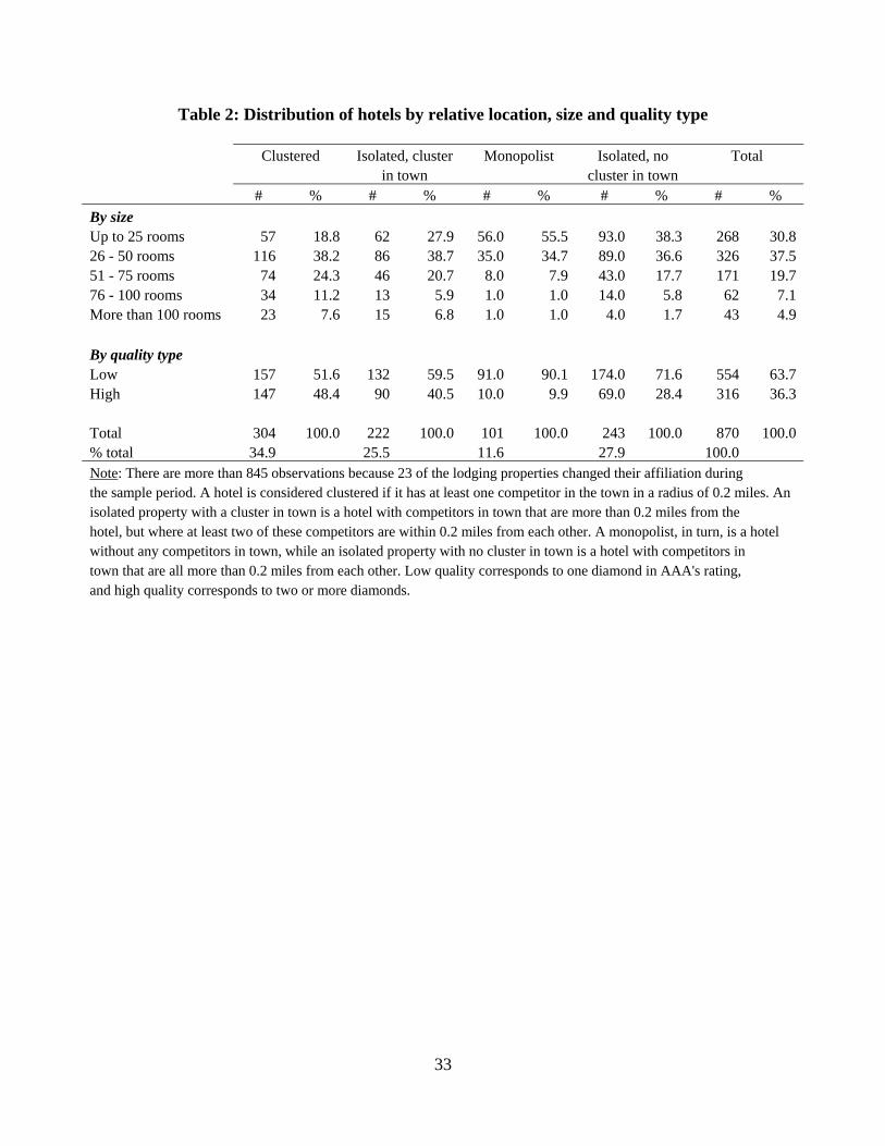
In Table 2 we report the distribution of hotels by their relative location, size and

quality type. Several patterns emerge from the table. First, the majority of the hotels in

our sample are small-sized properties, generally of low quality, which is consistent with

the small size of the markets considered for the analysis. In particular, 68% of the hotels

do not have more than 50 rooms, and 64% of the hotels are of low quality, i.e. are rated

with one diamond.18 Although not reported in the table, there is also a strong correlation

between low-quality type and independent hotels and small franchises. Second, 35% of

the hotels in our sample are clustered, i.e. have at least one nearby competitor in a radius

of 0.2 miles.19 This fraction decreases to 24% if we reduce the radius to 0.1 miles and

increases to 52% if we extend the radius to half a mile. Another 25% of the hotels do not

have a nearby competitor in a radius of 0.2 miles but face a cluster of hotels in town.

Finally, clustered hotels seem to be larger and of higher quality than the other groups of

hotels. Monopolists, in contrast, are much smaller and of lower quality, probably because

they are basically located in the smallest towns.

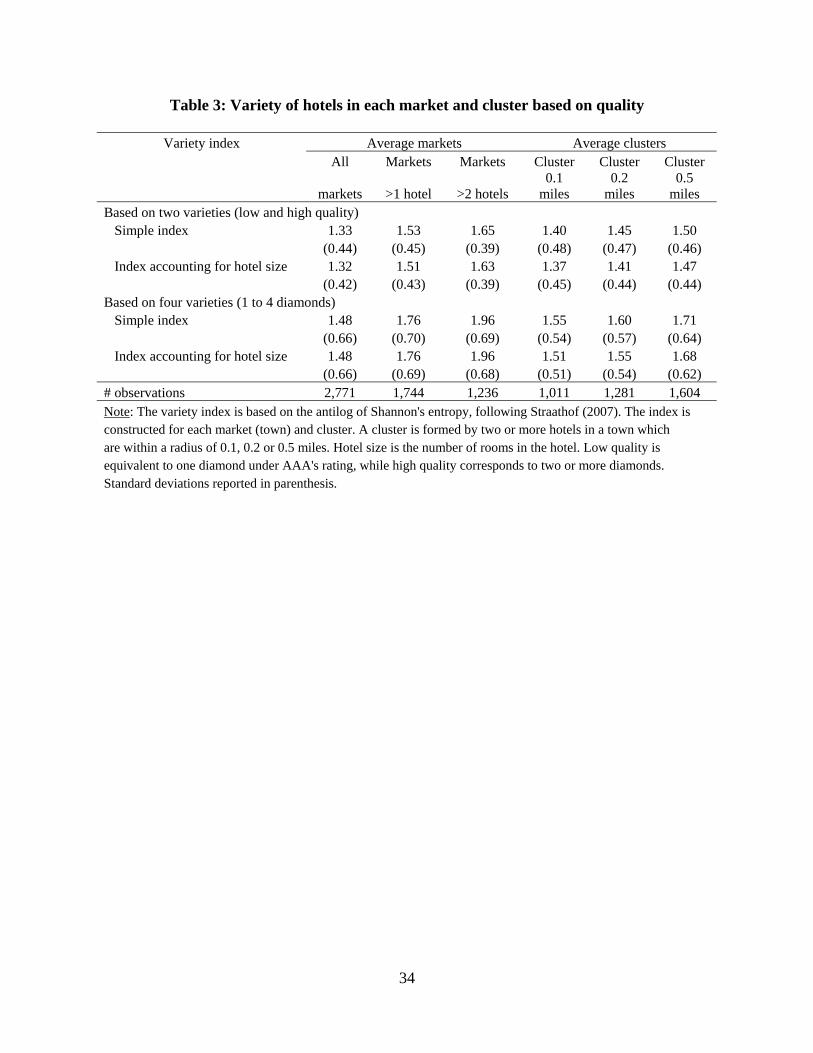
A closer look at the level of heterogeneity among hotels in a market and cluster

also confirms that the degree of product differentiation in our sample is very low. Table 3

reports average variety indexes based on hotel quality, both within a market (town) and

within a cluster. The index of product variety is the antilog of Shannon’s entropy,

following Straathof (2007). This index is preferred over the Gini coefficient because it

can be decomposed without losing its functional form, and has the property that it

18 Another 24% of the hotels in our sample have two diamonds, 12% have three diamonds, and only one hotel has four diamonds (Lajitas Golf Resort and Spa). 19 The average cluster size is 3.1 hotels.

13

reduces to the number of product types if all types have the same weight. We construct

both an index where each hotel in a market (cluster) has an equal weight and an index

that further takes into account the size of the hotel (number of rooms).20

When considering all markets (towns) in our sample, the average index is 1.32-

1.33 if we allow for two possible product varieties (low and high quality) and 1.48 if we

allow for four possible product varieties (one to four AAA’s diamonds). If we exclude

monopolistic markets from our sample, the index raises to 1.51-1.53 and 1.76,

respectively, while if we exclude markets with only one or two hotels, the corresponding

indexes are 1.63-1.65 and 1.96. These measures indicate that regardless of the number of

competitors, the markets are generally dominated by one type of product variety (the

average is less than two product varieties in all cases). Clusters also exhibit a low degree

of variety inside the cluster. The index ranges from 1.37 to 1.71 across the different

cluster radii considered for the analysis. Overall, this low level of heterogeneity among

hotels in our sample suggests that the risk of coordinated behavior is not necessarily low,

given that tacit collusion is easier to achieve when all firms offer similar products than

when they offer highly differentiated products. In the estimations, we still include this

variety index to account for potential complementarity or substitutability across hotels,

particularly among clustered hotels, as well as for hotel quality, chain affiliation and hotel

size as sources of product differentiation.

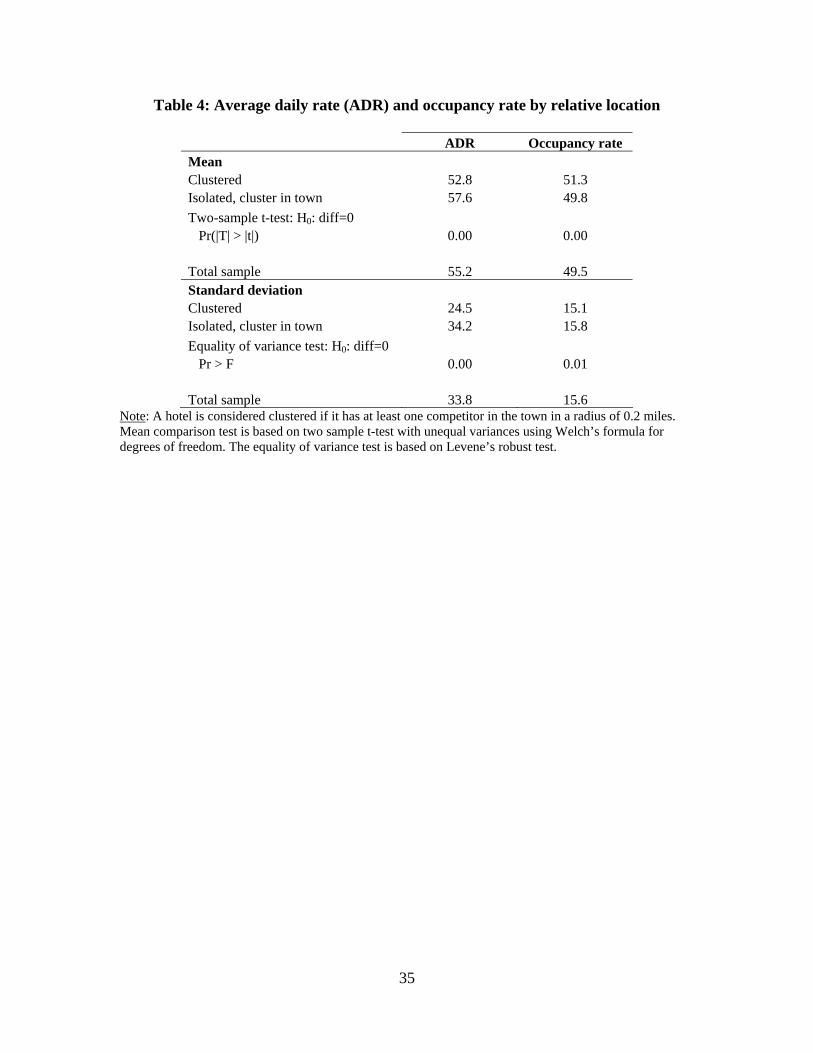
In this study, we are particularly interested in examining the price and occupancy

rate behavior of clustered hotels relative to isolated hotels in the same town. Figures 1

20 The variety index is defined as ∏ −=

N

wi

iwNV )( , where N is the total number of possible product

varieties (qualities) in a market, and wi is the weight of quality i, i=1,…,N. In this case, the weight may be the fraction of hotels of a specific quality or the fraction of rooms.

14

and 2 indicate that clustered hotels may behave differently from isolated properties.

Clustered hotels charge, on average, lower prices and have higher occupancy rates,

regardless of the season of the year. Overall, the average daily rate of a room in clustered

hotels is 52.8 dollars versus 57.6 dollars in isolated hotels with a cluster in town. The

average occupancy rate among clustered properties is 51.3%, and 49.8% among isolated

properties. The differences for both average daily rates and occupancy rates are

statistically significant at a one percent level, as shown in Table 4. In terms of dispersion,

clustered hotels exhibit a much lower dispersion in prices than isolated hotels with a

cluster in town, and a slightly lower dispersion in occupancy rates across the year. The

standard deviations for both prices and occupancy rates are also statistically significant

different at the one percent level (see Table 4).

This initial look at the data provides mixed support regarding the hypothesis that

agglomeration facilitates tacit collusion. If agglomeration increases the probability of

colluding and if there are not any deviations from the tacit collusive agreement (if any),

we would, then, expect a lower dispersion in prices and occupancy rates among clustered

properties, relative to isolated ones, as observed. However, we would also expect

clustered hotels to charge higher prices than isolated hotels and exhibit lower occupancy

rates, but not the inverse.21

Next, we formally examine whether agglomeration facilitates tacit collusion. We

propose a switching regression model to endogenously classify prices and occupancy 21 Alternatively, the differences in prices and occupancy rates between clustered and isolated hotels in a town could be explained in the context of spatial competition models, which considers a market power and a market share effect when clustering (e.g. Fujita and Thisse, 1996; Pinske and Slade, 1998; and Netz and Taylor, 2002). The market power effect predicts that, other things equal, firms will compete more intensively on prices when locating closer to each other (i.e. lower prices). But if the products between firms are differentiated enough, price competition may be weakened (Irmen and Thisse, 1998). The market share effect, in turn, predicts that firms will capture more customers when clustering (i.e. higher occupancy rates).

15

rates into a potential collusive and non-collusive regime, while controlling for several

factors at the property and market level that may affect a firm’s competitive behavior. We

then examine whether agglomerated hotels exhibit a higher probability of following the

potential collusive regime than isolated hotels in the same town.

4 The Empirical Model

This section develops a switching regime model to analyze if clustered hotels are more

likely to engage in tacit collusive behavior than isolated properties in the same town. We

jointly model a price and occupancy rate equation under a mixture modeling to

endogenously identify a collusive and non-collusive regime. We then analyze if

agglomeration increases the probability of colluding. As in Knittel and Stango (2003), we

also test whether our identification of the collusive regime is consistent with other factors

thought to affect the sustainability of tacit collusion.22

Let a firm’s log-linear price (p) and occupancy rate (q) equations be given by,

simt

simtmt

ssimt XreMktStructup εγδδ +++= 21ln and (2)

simt

simtmt

ssimt uXreMktStructuq +++= βαα 21ln , (3)

where the subscript i refers to a firm, m to the market, and t to the time period, and the

superscript s indicates one of two possible regimes, a collusive regime (C) and a non-

collusive one (NC). The variable MktStructuremt measures the level of concentration in

the market through the Herfindahl-Hirshman Index (HHI), which is based on each firm’s

22 These authors point out that an omitted variable or misspecification of the functional form might lead to the spurious identification of two regimes, a collusive and a non-collusive one. They suggest, then, to examine whether the probability of being in the identified collusive regime varies with factors thought to affect the sustainability of tacit collusion.

16

share of rooms sold, and the vector Ximt includes several property- and market-specific

variables. The summary statistics of all variables used in the estimations are presented in

Table 5.

The property-specific variables include dummy variables for the geographic

location of hotels relative to their nearby competitors (i.e. clustered, isolated with a

cluster of hotels in town, monopolist, isolated with no cluster in town), cluster size,

number of other hotels in the cluster of similar quality, cluster heterogeneity measured

through a variety index based on hotel quality (1-4 diamonds), a dummy variable if the

hotel is of medium or large size (i.e. if the hotel has more than 50 rooms), and dummy

variables for high-quality and affiliations to major chains in our sample.23 These control

variables are intended to account for possible sources of product differentiation (hotel

quality, size and chain affiliation), the degree of complementarity or substitutability

across nearby hotels (number of hotels of similar quality, variety index), and for potential

agglomeration and spatial competition effects (whether clustered and cluster size).

The market-specific variables, which have been generally used in other studies,

include population, per capita personal income, number of gas stations, value of rural

land per acre, wage on leisure and hospitality, distance to a MSA, distance to the closest

town, and regional dummies. These firm- and market-specific variables are supposed to

account for cost and demand factors that may affect a firm’s competitive behavior,

besides market concentration. Per capita personal income and population, for example,

could be positively correlated with hotel demand in the sense that wealthier and larger

towns usually have more businesses and people to visit. The number of gas stations in

23 The major chains include Best Western, Best Value, Comfort, Days, Econolodge, Holiday, Motel 6, Super 8 and Ramada.

17

area, which could serve as a proxy for travelers passing through and visiting an area,

should also be correlated with hotel demand.24 Wages and the value of land are expected

to account for firm costs, while a higher distance to a MSA or to the next closest town

could be associated with a higher demand and/or higher market power in the vicinity of

the area.

We can further assume that the error terms in each regime s, },{ NCCs = , are

bivariate normally distributed such that ),,,0,0(~),( 222 s

su

ssimt

simt Nu ρσσε ε where

su

s

su

s σσσ

ρε

ε= . Then, the log likelihood for the jth firm-quarter period can be modeled as,

⎟⎟

⎠

⎞

⎟⎟⎠

⎞⎜⎜⎝

⎛

−

−

−−+

⎜⎜

⎝

⎛

⎟⎟⎠

⎞⎜⎜⎝

⎛

−

−

−=

)1(2exp

121)1(

)1(2exp

12

1lnln

22

22

NC

NCj

NCNCu

NC

C

Cj

CCu

Cj

zh

zhl

ρρσπσ

ρρσπσ

ε

ε (4)

where su

s

sj

sj

s

su

sj

s

sjs

j

uuz

σσερ

σσε

εε

22

2

2

2

−+= and the mixing parameter h, ]1,0[∈h , is defined as

the probability that a firm will tacitly collude.

In the collusive regime, firms are expected to charge higher prices, which also

result in lower occupancy rates than in the non-collusive regime. Additionally, during

successful periods of tacit collusion we expect a lower dispersion in prices and

occupancy rates. Identifying a potential collusive regime, then, requires to test if

NCC11 δδ > , NCC

11 αα < , NCCεε ασ < , and NC

uCu ασ < .

24 Gas stations exist to serve both residents of and travelers passing through and visiting a market. As suggested by Chung and Kalnins (2001), a higher number of gas stations in a market might also indicate that the area is well located as an intermediate point from one major destination to another.

18

Note that in the empirical framework above the two identified regimes do not

necessarily correspond to two fixed time periods. Furthermore, hotels may or may not

alternate between the two regimes. Switching from a collusive to a non-collusive regime

may occur, if any, when a firm cheats or deviates from the tacit collusive path and

triggers some retaliation by the other firms involved in the tacit agreement (reversion

period). Identifying, however, the exact pattern of collusive and non-collusive and/or

retaliation periods (if any) is beyond the scope of the study due to the nature of our data

(quarterly data); retaliation periods, for example, could last less or more than a quarter.

We focus on deriving the probability of being in the potential collusive and

examining the factors that drive this probability, particularly whether being clustered.

We model the mixing parameter h or probability of engaging in tacit collusion both as a

constant, but allowing for variations in certain regions due to unobserved market factors

intrinsic to these regions, and as a function of the geographical location of a hotel relative

to its nearby competitors. In the first case, )( 23121 RRGh κκκ ++= where 1R is a

dummy variable equal to one if the hotel is located in Central Texas or the Metroplex

(upper Central Texas), 2R equals one if the hotel is located in the South or the Gulf

Coast, and )(⋅G is approximated with a logistic CDF.25 In the second case,

)__( 26154321 RRclusternoIsolatedMonopClusteredGh jjjj κκκκκκ +++++= where

Clustered equals one if the hotel has at least one nearby competitor in the town in a

radius of 0.2 miles, Monop equals one if the hotel is the only one operating in the town,

and Isolated_no_cluster equals one for hotels with competitors in town that are all more

25 These regions are also clearly the most important in the state in terms of visitor spending (State of Texas: Economic Development and Tourism Office, www.governor.state.tx.us/ecodev/)

19

than 0.2 miles apart from each other.26 The first specification assumes that the probability

of tacit collusion is constant across hotels but may vary by specific regions, while the

second specification further allows us to evaluate whether the probability of being in a

potential collusive regime varies with the relative location of the hotel within the town.

Examining then if agglomeration facilitates collusion is equivalent to testing if 02 >κ .

Provided that our identification strategy of a collusive and non-collusive regime

may be subject to an omitted variable or misspecification of the functional form, we also

model h as a function of other factors typically correlated with the sustainability of tacit

collusion. The idea is to reduce the possibility of alternative explanations for the results

obtained. These other factors include cluster size, seasonality and firm size. Tacit

collusion is easier to maintain among fewer firms so the probability of being in a

potential collusive regime should decrease with the number of firms in the cluster.

Similarly, collusion is less likely during high season periods because the gain from

cheating during a peak-demand period is higher than the future punishment (Rotemberg

and Saloner, 1986).27 Finally, the probability of colluding should also increase with firm

size since deviations from any tacit collusive agreement are typically more profitable for

smaller than for larger firms.28

In the estimation of the price and occupancy rate equations specified in (2) and

(3), some of the right-hand side variables are likely to be endogenous. In particular, the

26 The dummy variable for isolated properties with a cluster of hotels in town is the base category. 27 Alternatively, if both current demand and firms’ expectations on future demand are allowed to change over time, it will be more difficult for firms to collude when demand is falling (i.e. during low seasons) since the foregone profits from inducing a price war are relatively low (Haltiwanger and Harrington, 1991). 28 Smaller firms, however, may also have less to gain from undercutting their rivals because of their higher capacity constraints relative to larger firms. But hotels in rural areas, at least in Texas, seem to operate well below their capacity (at around 50%). As noted by Kalnins (2006), the nationwide occupancy rate of an average hotel is roughly 60% while the break-even occupancy (i.e. percentage of rooms that must be sold on average for a hotel to show positive pretax income) is roughly estimated at 53%.

20

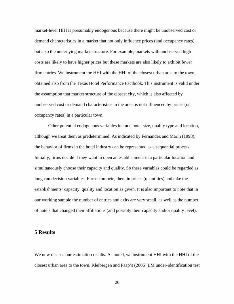
market-level HHI is presumably endogenous because there might be unobserved cost or

demand characteristics in a market that not only influence prices (and occupancy rates)

but also the underlying market structure. For example, markets with unobserved high

costs are likely to have higher prices but these markets are also likely to exhibit fewer

firm entries. We instrument the HHI with the HHI of the closest urban area to the town,

obtained also from the Texas Hotel Performance Factbook. This instrument is valid under

the assumption that market structure of the closest city, which is also affected by

unobserved cost or demand characteristics in the area, is not influenced by prices (or

occupancy rates) in a particular town.

Other potential endogenous variables include hotel size, quality type and location,

although we treat them as predetermined. As indicated by Fernandez and Marin (1998),

the behavior of firms in the hotel industry can be represented as a sequential process.

Initially, firms decide if they want to open an establishment in a particular location and

simultaneously choose their capacity and quality. So these variables could be regarded as

long-run decision variables. Firms compete, then, in prices (quantities) and take the

establishments’ capacity, quality and location as given. It is also important to note that in

our working sample the number of entries and exits are very small, as well as the number

of hotels that changed their affiliations (and possibly their capacity and/or quality level).

5 Results

We now discuss our estimation results. As noted, we instrument HHI with the HHI of the

closest urban area to the town. Kleibergen and Paap’s (2006) LM under-identification test

21

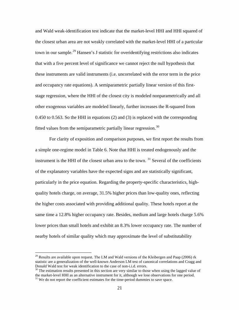
and Wald weak-identification test indicate that the market-level HHI and HHI squared of

the closest urban area are not weakly correlated with the market-level HHI of a particular

town in our sample.29 Hansen’s J statistic for overidentifying restrictions also indicates

that with a five percent level of significance we cannot reject the null hypothesis that

these instruments are valid instruments (i.e. uncorrelated with the error term in the price

and occupancy rate equations). A semiparametric partially linear version of this first-

stage regression, where the HHI of the closest city is modeled nonparametrically and all

other exogenous variables are modeled linearly, further increases the R-squared from

0.450 to 0.563. So the HHI in equations (2) and (3) is replaced with the corresponding

fitted values from the semiparametric partially linear regression.30

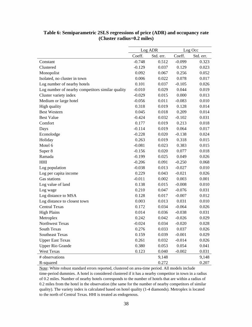
For clarity of exposition and comparison purposes, we first report the results from

a simple one-regime model in Table 6. Note that HHI is treated endogenously and the

instrument is the HHI of the closest urban area to the town. 31 Several of the coefficients

of the explanatory variables have the expected signs and are statistically significant,

particularly in the price equation. Regarding the property-specific characteristics, high-

quality hotels charge, on average, 31.5% higher prices than low-quality ones, reflecting

the higher costs associated with providing additional quality. These hotels report at the

same time a 12.8% higher occupancy rate. Besides, medium and large hotels charge 5.6%

lower prices than small hotels and exhibit an 8.3% lower occupancy rate. The number of

nearby hotels of similar quality which may approximate the level of substitutability

29 Results are available upon request. The LM and Wald versions of the Kleibergen and Paap (2006) rk statistic are a generalization of the well-known Anderson LM test of canonical correlations and Cragg and Donald Wald test for weak identification to the case of non-i.i.d. errors. 30 The estimation results presented in this section are very similar to those when using the lagged value of the market-level HHI as an alternative instrument for it, although we lose observations for one period. 31 We do not report the coefficient estimates for the time-period dummies to save space.

22

between hotels and their nearby competitors, does not affect prices, but has a positive

effect on occupancy rates.

With respect to the market-specific variables, market concentration has a negative

effect on prices, and does not significantly affect occupancy rates. A one standard

deviation decrease in the HHI (0.28) results in a 5.2% increase in prices. This result

might seem counterintuitive but in certain oligopolistic models the “displacement effect”

may dominate the “competitive effect” with increased competition, which will result in

higher prices (Satterthwaite, 1979; Rosenthal, 1980; Sutton, 1991).32 Prices are also

positively correlated with the per capita income in the area. This is in line with the fact

that wealthier locations usually have more businesses and places to visit, so we expect a

higher number of visitors and higher prices. Hotels located in areas with higher wages

and a higher value of land naturally charge higher prices because of the higher costs they

face. Additionally, distance to a MSA is positively correlated with prices, while a larger

distance between towns involves higher occupancy rates. Curiously, population has a

negative (although economically small) effect on both prices and occupancy rates.

Finally, a higher number of gas stations in the area, which may approximate potential

demand for hotel rooms, have a positive effect on occupancy rates but a negative impact

on prices.

We now turn to the MLE results of the switching regression model, which

endogenously classifies prices and occupancy rates into two regimes. As noted above, we

jointly model a price and occupancy rate equation under each regime, and the two

32 Intuitively, in oligopolistic models where sellers have both a captive and a free-entry market, an increase in the number of sellers can reduce the probability that a seller will attract more customers, decreasing their demand elasticity for the average expected customer, and increasing their price. Empirically, a similar negative relationship between concentration and prices has been found in other industries with oligopolistic competition like the airline industry (Borenstein, 1989; Stavins, 2001).

23

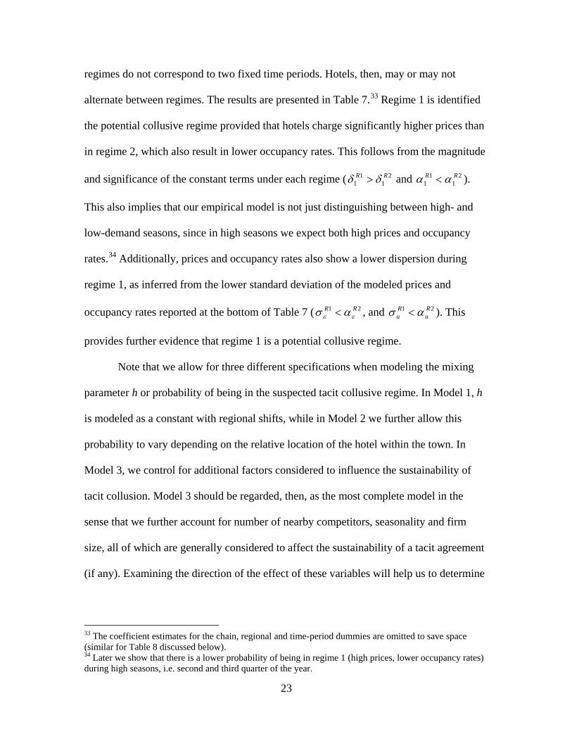
regimes do not correspond to two fixed time periods. Hotels, then, may or may not

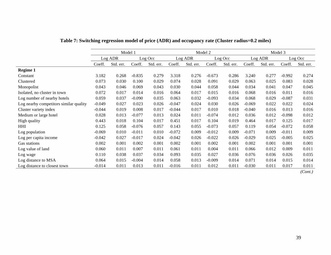
alternate between regimes. The results are presented in Table 7.33 Regime 1 is identified

the potential collusive regime provided that hotels charge significantly higher prices than

in regime 2, which also result in lower occupancy rates. This follows from the magnitude

and significance of the constant terms under each regime ( 21

11

RR δδ > and 21

11

RR αα < ).

This also implies that our empirical model is not just distinguishing between high- and

low-demand seasons, since in high seasons we expect both high prices and occupancy

rates.34 Additionally, prices and occupancy rates also show a lower dispersion during

regime 1, as inferred from the lower standard deviation of the modeled prices and

occupancy rates reported at the bottom of Table 7 ( 21 RRεε ασ < , and 21 R

uRu ασ < ). This

provides further evidence that regime 1 is a potential collusive regime.

Note that we allow for three different specifications when modeling the mixing

parameter h or probability of being in the suspected tacit collusive regime. In Model 1, h

is modeled as a constant with regional shifts, while in Model 2 we further allow this

probability to vary depending on the relative location of the hotel within the town. In

Model 3, we control for additional factors considered to influence the sustainability of

tacit collusion. Model 3 should be regarded, then, as the most complete model in the

sense that we further account for number of nearby competitors, seasonality and firm

size, all of which are generally considered to affect the sustainability of a tacit agreement

(if any). Examining the direction of the effect of these variables will help us to determine

33 The coefficient estimates for the chain, regional and time-period dummies are omitted to save space (similar for Table 8 discussed below). 34 Later we show that there is a lower probability of being in regime 1 (high prices, lower occupancy rates) during high seasons, i.e. second and third quarter of the year.

24

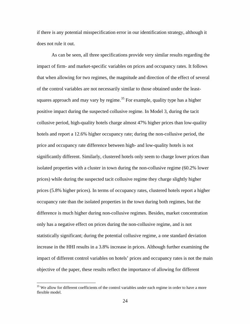
if there is any potential misspecification error in our identification strategy, although it

does not rule it out.

As can be seen, all three specifications provide very similar results regarding the

impact of firm- and market-specific variables on prices and occupancy rates. It follows

that when allowing for two regimes, the magnitude and direction of the effect of several

of the control variables are not necessarily similar to those obtained under the least-

squares approach and may vary by regime.35 For example, quality type has a higher

positive impact during the suspected collusive regime. In Model 3, during the tacit

collusive period, high-quality hotels charge almost 47% higher prices than low-quality

hotels and report a 12.6% higher occupancy rate; during the non-collusive period, the

price and occupancy rate difference between high- and low-quality hotels is not

significantly different. Similarly, clustered hotels only seem to charge lower prices than

isolated properties with a cluster in town during the non-collusive regime (60.2% lower

prices) while during the suspected tacit collusive regime they charge slightly higher

prices (5.8% higher prices). In terms of occupancy rates, clustered hotels report a higher

occupancy rate than the isolated properties in the town during both regimes, but the

difference is much higher during non-collusive regimes. Besides, market concentration

only has a negative effect on prices during the non-collusive regime, and is not

statistically significant; during the potential collusive regime, a one standard deviation

increase in the HHI results in a 3.8% increase in prices. Although further examining the

impact of different control variables on hotels’ prices and occupancy rates is not the main

objective of the paper, these results reflect the importance of allowing for different

35 We allow for different coefficients of the control variables under each regime in order to have a more flexible model.

25

regimes when analyzing marginal effects of firm- and market-specific characteristics on

hotels’ competitive behavior.

Moving to the likelihood of being in regime 1, the potential collusive regime, in

Model 1 we observe that the sample-wide probability is equal to 70.9%.36 Note that the

probability of engaging in tacit collusion is lower for properties located in both Central

Texas and the Metroplex (upper Central Texas) and South Texas and the Gulf Coast,

areas with a more developed lodging industry than other rural regions in the state. When

we further allow in Model 2 for the probability to vary with the geographical location of

hotels, relative to their local competitors, we find that clustered hotels have a higher

probability of engaging in tacit collusion than isolated properties in the town (base

group). In particular, hotels with nearby competitors in a radius of 0.2 miles have a 10

percentage-point higher probability of being in regime 1 than isolated properties (78%

versus 68%). Monopolists, whose behavior should resemble perfect collusion, are also

more likely of being in the potential collusive regime than isolated properties with a

cluster in town, while isolated hotels without a cluster in town show a lower probability.

If we further control for cluster size, seasonality and firm size, we still find that

clustered hotels and monopolists have a higher probability of being in the potential

collusive regime while isolated properties without a cluster in town have a lower

probability (Model 3). Clustered hotels exhibit a 70% probability of being in the collusive

regime, other things constant, while isolated hotels with a cluster in town only show a

63% probability. Monopolists have a 73% probability of being in regime 1, while isolated

hotels without a cluster in town show a 55% probability. At the sample means, then,

36 From the regression,

%9.70))792.0976.0321.1exp(1()792.0976.0321.1exp( 2121 =−−+−−= RRRRh .

26

monopolists are the most likely to be in the potential collusive regime; however, when

converting the estimated probabilities for each hotel in our sample to binary regime

predictions, using the standard 0.5 rule, we find that all monopolists are predicted to

follow the potential collusive regime, in contrast with the other types of hotels. So,

regardless of the flexibility of our model, where hotels are allowed to follow two regimes,

all monopolistic hotels in our sample are always predicted to be in the collusive regime

(as expected), which provides further evidence in favor of our identification strategy.

The direction of the coefficients of the other control variables is also consistent

with the discussion of factors, other than agglomeration, considered to affect the

sustainability of collusion. The likelihood of tacit collusion decreases with the number of

hotels in the cluster provided that it is easier to collude among fewer firms; decreases

during high seasons given that collusion is more difficult to maintain during high-demand

periods (Rotemberg and Saloner, 1986); and increases with hotel size provided that

deviations from a collusive agreement are less profitable for large firms.37 Figure 3

illustrates the effects of these other variables by plotting the estimated probability of

colluding, conditional on being clustered, as a function of the number of hotels in the

cluster and by seasonality and hotel size.

In sum, the results suggest that agglomeration facilitates tacit collusion. Clustered

hotels show a higher probability of being in the potential collusive regime than isolated

hotels in the same town. Our identification of the collusive regime is also consistent with

other factors thought to affect the sustainability of colluding. Furthermore, monopolists,

37The fact that small firms are less likely of being in the potential collusive regime also suggests that small firms are not necessarily following the behavior of large firms, which reduces the possibility of umbrella pricing. The same reasoning applies when analyzing the behavior of isolated properties relative to clustered hotels in the same town: isolated hotels (the outside firms) have a lower probability of being in the collusive regime relative to clustered hotels (the potential colluding firms).

27

whose behavior should resemble perfect collusion, are always predicted to fall in the tacit

collusive regime.

As a robustness check, we examine whether these findings persist under

alternative cluster definitions. We consider a cluster radius of 0.1 miles and a cluster

radius of 0.5 miles. The results are presented in Table 8 where regime 1 is again the

potential collusive regime with higher prices, lower occupancy rates and a lower

dispersion in both market outcomes, relative to regime 2, as inferred from the constant

terms and the estimated standard deviations of the price and occupancy rate equations.

Note that the estimated coefficients of the control variables under the two alternative

cluster definitions are very similar to the ones obtained with a cluster radius of 0.2 miles

(Model 3 in Table 7).

If we either restrict the cluster radius to 0.1 miles or expand the cluster radius to

0.5 miles, we still observe that clustered hotels have a higher probability of engaging in

tacit collusion than isolated properties with a cluster in town. In the case of a cluster

radius of 0.1 miles, holding all else constant, clustered hotels have a 73% probability of

being in the potential collusive regime versus 62% for isolated properties with a cluster in

town; in the case of a cluster radius of 0.5 miles, the probabilities are 69% versus 51%,

respectively.38 Monopolists also exhibit the highest probability of being in the collusive

regime at the sample means, and are always predicted to fall in the potential collusive

regime when converting the estimated probabilities to binary regime predictions.

38 It is interesting to observe that, on average, the probability for a clustered hotel to engage in tacit collusion decreases as we increase the cluster radius: 73% in a cluster radius of 0.1 miles, 70% in a radius of 0.2 miles and 69% in a radius of 0.5 miles. According to the tacit collusion theory, the likelihood of engaging in a collusive agreement decreases with higher monitor costs. This finding supports to some extent, then, the hypothesis that monitoring costs are lower for clustered hotels (particularly among those located sufficiently close to one another) than for hotels located farther apart.

28

Additionally, the likelihood of being in the identified collusive regime is negatively

correlated with cluster size and high-demand seasons, and positively correlated with firm

size. Figure 4, for example, shows that the probability of tacitly colluding, conditional on

being clustered, is decreasing in cluster size for the different cluster definitions.

6 Conclusions

This paper has empirically examined whether if agglomeration facilitates tacit collusion

in the lodging industry using a quarterly dataset of hotels that operated in rural areas

across Texas between 2003 and 2005. Unlike previous studies that use some form of

mixture modeling and focus on price behavior, we jointly model a price and occupancy

rate equation under a switching regression model to endogenously identify a collusive

and non-collusive regime. Hotels in our sample may follow a particular regime or

alternate between regimes across time. In the potential collusive regime, hotels are

expected to charge higher prices and exhibit lower occupancy rates than in the non-

collusive regime, and both prices and occupancy rates are expected to show a lower

dispersion. We focus on analyzing whether agglomeration increases the probability of

being in the collusive regime.

The results indicate that clustered hotels have a higher probability of being in the

potential collusive regime than isolated hotels with a cluster in town. In particular, hotels

with nearby competitors in a radius of 0.2 miles are about ten percentage points more

likely of being in the collusive regime than isolated properties in the same town. Our

identification of a collusive regime is also consistent with other factors considered to

29

affect the sustainability of tacit collusion like cluster size, seasonality and firm size, and

the results are robust to alternative cluster definitions. Further, monopolists, whose

behavior should resemble perfect collusion, are always predicted to fall in the potential

collusive regime when deriving binary regime predictions using the standard 0.5 rule.

These findings support the hypothesis that agglomeration may facilitate tacit

collusion among clustered hotels (if any) by providing additional opportunities for

frequent interaction and exchange of information among hotel managers, and by reducing

monitoring costs and increasing market transparency. We recognize that the inclusion of

other variables thought to affect the sustainability of collusion cannot completely rule out

any potential misspecification error in our identification strategy, but reduces the

possibility of alternative explanations for the results obtained. The nature of our dataset

(i.e. quarterly data) also prevents us from identifying the exact pattern of collusive and

non-collusive and/or retaliation periods followed by hotels. It further limits the possibility

of considering alternative identification strategies, like allowing for reversion periods

during the collusive regime. Similarly, we take long-run decision variables like capacity,

quality and geographic location as given due to the small number of entries/exits and

change of affiliations in our sample. Future research should incorporate dynamic aspects

into the analysis of agglomeration and tacit collusion.

30

References

Abrantes-Metz, Rosa M., Luke M. Froeb, John F. Geweke, and Christopher T. Taylor, “A

variance screen for collusion,” International Journal of Industrial Organization 24:3 (2006), 467-486.

Athey, Susan, Kyle Bagwell, and Chris Sanchirico, “Collusion and Price Rigidity,” Review of Economic Studies 71:2 (2004), 317-349.

Baum, Joel A. C., and Heather A. Haveman, “Love Thy Neighbor? Differentiation and Agglomeration in the Manhattan Hotel Industry, 1898-1990,” Administrative Science Quarterly 42:2 (1997), 304-338.

Borenstein, Severin, ‘Hubs and High Fares: Dominance and Market Power in the U.S. Airline Industry,” RAND Journal of Economics, 20:3 (1989), 344-365.

Bresnahan, Timothy F., and Peter C. Reiss, “Entry and Competition in Concentrated Markets,” Journal of Political Economy 99:5 (1991), 977-1009.

Connor, John M., “Collusion and price dispersion,” Applied Economics Letters 12:6 (2005), 335-338.

Chung, Wilbur, and Arturs Kalnins, “Agglomeration Effects and Performance: A Test of the Texas Lodging Industry,” Strategic Management Journal 22:10 (2001), 969-988.

Ellison, Glenn, “Theories of Cartel Stability and the Joint Executive Committee,” RAND Journal of Economics 25:1 (1994), 37-57.

Fernandez, Nerea and Pedro L. Marin, “Market Power and Multimarket Contact: Some Evidence from the Spanish Hotel Industry,” Journal of Industrial Economics 46:3 (1998), 301-315.

Fischer, Jeffrey H., and Joseph E. Harrington Jr., “Product Variety and Firm Agglomeration,” RAND Journal of Economics 27:2 (1996), 281-309.

Friedman, James W., and Jacques-Francois Thisse, “Infinite Horizon Spatial Duopoly with Collusive Pricing and Noncollusive Location Choice,” CORE Discussion Paper No. 9104, Universite Catholique de Louvain (1991).

Fujita, Masahisa, and Jacques-Francois Thisse, “Economics of Agglomeration,” Journal of the Japanese and International Economies 10:4 (1996), 339-378.

______, Economics of Agglomeration: Cities, Industrial Location, and Regional Growth, Cambridge University Press (2002).

Haltiwanger, John, and Joseph E. Harrington Jr., “The Impact of Cyclical Demand Movements on Collusive Behavior,” RAND Journal of Economics 22:1 (1991), 89-106.

Harrington, Joseph E., “Detecting Cartels,” Working paper John Hopkins University (2005).

Helsley, Robert W., and William C. Strange, “Matching and Agglomeration Economies in a System of Cities,” Regional Science and Urban Economics 20:2 (1990), 189-212.

Irmen, Andreas, and Jacques-Francois Thisse, “Competition in Multi-characteristics Spaces: Hotelling was Almost Right,” Journal of Economic Theory 78:1 (1998), 76-102.

31

Ivaldi, Marc, Bruno Jullien, Patrick Rey, Paul Seabright, and Jean Tirole, “The Economics of Tacit Collusion,” Final Report for DG Competition, European Commission (2003).

Kalnins, Arturs, “The U.S. Lodging Industry,” Journal of Economic Perspectives 20:4 (2006), 203-218.

Kalnins, Arturs, and Wilbur Chung, “Resource-Seeking Agglomeration: A Study of Market Entry in the Lodging Industry,” Strategic Management Journal 25:7 (2004), 689-699.

Kleibergen, Frank, and Richard Paap, “Generalized reduced rank tests using the singular value decomposition,” Journal of Econometrics 133:1 (2006), 97-126.

Knittel, Christopher R., and Victor Stango, “Price Ceilings as Focal Points for Tacit Collusion: Evidence from Credit Cards,” American Economic Review 93:5 (2003), 1703-1729.

Mazzeo, Michael, “Competitive Outcomes in Product-Differentiated Oligopoly,” Review of Economics and Statistics 84:4 (2002), 716-728.

Netz, Janet S., and Beck A. Taylor, “Maximum or Minimum Differentiation? Location Patterns of Retail Outlets,” Review of Economics and Statistics 84:1 (2002), 162-175.

Pinkse, Joris, and Margaret E. Slade, “Contracting in Space: An application of spatial statistics to discrete choice models,” Journal of Econometrics 85:1 (1998), 125-154.

Porter, Robert H., “A Study of Cartel Stability: The Joint Executive Committee, 1880-1886,” Bell Journal of Economics 14:2 (1983), 301-314.

Rosenthal, Robert W., “A Model in Which An Increase in the Number of Sellers Leads to a Higher Price,” Econometrica 48:6 (1980), 1575-1579.

Rotemberg, Julio J., and Garth Saloner, “A Supergame-Theoretic Model of Price Wars during Booms,” American Economic Review 76:3 (1986), 390-407.

Satterthwaite, Mark A., “Consumer Information, Equilibrium Industry Price, and the Number of Sellers,” Bell Journal of Economics 10:2 (1979), 483-502.

Stahl, Konrad, “Differentiated Products, Consumer Search, and Locational Oligopoly,” Journal of Industrial Economics 31:1/2 (1982), 97-113.

Stavins, Joanna, “Price Discrimination in the Airline Market: The Effect of Market Concentration,” Review of Economics and Statistics 83:1 (2001), 200-202.

Straathof, Sebastiaan M., “Shannon’s Entropy as an Index of Product Variety,” Economics Letters 94:2 (2007), 297-303.

Sutton, John, Sunk Costs and Market Structure, The MIT Press (1991). Tirole, Jean, The Theory of Industrial Organization, The MIT Press (1988). Wolinsky, Asher, “Retail Trade Concentration due to Consumers’ Imperfect

Information,” Bell Journal of Economics 14:1 (1983), 275-282.

32

Table 1: Distribution of markets by number of hotels

# hotels in # markets % market

1 1,027 37.1 2 508 18.3 3 380 13.7 4 133 4.8 5 204 7.4 6 129 4.7 7 79 2.9 8 55 2.0 9 68 2.5 10 56 2.0 More than 10 132 4.8 Total 2,771 100.0

33

Table 2: Distribution of hotels by relative location, size and quality type

Clustered Isolated, cluster Monopolist Isolated, no Total in town cluster in town # % # % # % # % # % By size Up to 25 rooms 57 18.8 62 27.9 56.0 55.5 93.0 38.3 268 30.8 26 - 50 rooms 116 38.2 86 38.7 35.0 34.7 89.0 36.6 326 37.5 51 - 75 rooms 74 24.3 46 20.7 8.0 7.9 43.0 17.7 171 19.7 76 - 100 rooms 34 11.2 13 5.9 1.0 1.0 14.0 5.8 62 7.1 More than 100 rooms 23 7.6 15 6.8 1.0 1.0 4.0 1.7 43 4.9 By quality type Low 157 51.6 132 59.5 91.0 90.1 174.0 71.6 554 63.7 High 147 48.4 90 40.5 10.0 9.9 69.0 28.4 316 36.3 Total 304 100.0 222 100.0 101 100.0 243 100.0 870 100.0 % total 34.9 25.5 11.6 27.9 100.0 Note: There are more than 845 observations because 23 of the lodging properties changed their affiliation during the sample period. A hotel is considered clustered if it has at least one competitor in the town in a radius of 0.2 miles. An isolated property with a cluster in town is a hotel with competitors in town that are more than 0.2 miles from the hotel, but where at least two of these competitors are within 0.2 miles from each other. A monopolist, in turn, is a hotel without any competitors in town, while an isolated property with no cluster in town is a hotel with competitors in town that are all more than 0.2 miles from each other. Low quality corresponds to one diamond in AAA's rating, and high quality corresponds to two or more diamonds.

34

Table 3: Variety of hotels in each market and cluster based on quality

Variety index Average markets Average clusters All Markets Markets Cluster Cluster Cluster

markets >1 hotel >2 hotels 0.1

miles 0.2

miles 0.5

miles Based on two varieties (low and high quality) Simple index 1.33 1.53 1.65 1.40 1.45 1.50 (0.44) (0.45) (0.39) (0.48) (0.47) (0.46) Index accounting for hotel size 1.32 1.51 1.63 1.37 1.41 1.47 (0.42) (0.43) (0.39) (0.45) (0.44) (0.44) Based on four varieties (1 to 4 diamonds) Simple index 1.48 1.76 1.96 1.55 1.60 1.71 (0.66) (0.70) (0.69) (0.54) (0.57) (0.64) Index accounting for hotel size 1.48 1.76 1.96 1.51 1.55 1.68 (0.66) (0.69) (0.68) (0.51) (0.54) (0.62) # observations 2,771 1,744 1,236 1,011 1,281 1,604 Note: The variety index is based on the antilog of Shannon's entropy, following Straathof (2007). The index is constructed for each market (town) and cluster. A cluster is formed by two or more hotels in a town which are within a radius of 0.1, 0.2 or 0.5 miles. Hotel size is the number of rooms in the hotel. Low quality is equivalent to one diamond under AAA's rating, while high quality corresponds to two or more diamonds. Standard deviations reported in parenthesis.

35

Table 4: Average daily rate (ADR) and occupancy rate by relative location

ADR Occupancy rate Mean Clustered 52.8 51.3 Isolated, cluster in town 57.6 49.8 Two-sample t-test: H0: diff=0 Pr(|T| > |t|) 0.00 0.00 Total sample 55.2 49.5 Standard deviation Clustered 24.5 15.1 Isolated, cluster in town 34.2 15.8 Equality of variance test: H0: diff=0 Pr > F 0.00 0.01 Total sample 33.8 15.6

Note: A hotel is considered clustered if it has at least one competitor in the town in a radius of 0.2 miles. Mean comparison test is based on two sample t-test with unequal variances using Welch’s formula for degrees of freedom. The equality of variance test is based on Levene’s robust test.

36

Table 5: Summary statistics for variables used in the analysis

Mean St. dev. Min Max ADR (US$) 55.2 33.8 17.5 524.2 Occupancy rate 0.50 0.16 0.02 0.98 Firm variables Clustered, cluster radius=0.2 miles 0.35 0.48 0.00 1.00 Isolated, cluster in town 0.26 0.44 0.00 1.00 Monopolist 0.11 0.32 0.00 1.00 Isolated, no cluster in town 0.27 0.44 0.00 1.00 Number of nearby hotels in a radius of 0.2 miles 1.76 1.40 1.00 9.00 Number of nearby competitors of similar quality in a radius of 0.2 miles 0.47 1.12 0.00 8.00 Cluster variety index based on hotel quality, cluster radius=0.2 miles 1.25 0.49 1.00 3.00 Clustered, cluster radius=0.1 miles 0.25 0.43 0.00 1.00 Number of nearby hotels in a radius of 0.1 miles 1.38 0.79 1.00 6.00 Number of nearby competitors of similar quality in a radius of 0.1 miles 0.26 0.69 0.00 5.00 Cluster variety index based on hotel quality, cluster radius=0.1 miles 1.15 0.38 1.00 3.00 Clustered, cluster radius=0.5 miles 0.53 0.50 0.00 1.00 Number of nearby hotels in a radius of 0.5 miles 2.75 2.68 1.00 14.00 Number of nearby competitors of similar quality in a radius of 0.5 miles 1.01 1.76 0.00 9.00 Cluster variety index based on hotel quality, cluster radius=0.5 miles 1.48 0.65 1.00 3.00 Medium or large hotel 0.32 0.47 0.00 1.00 High quality 0.37 0.48 0.00 1.00 Best Western 0.09 0.29 0.00 1.00 Best Value 0.01 0.11 0.00 1.00 Comfort 0.03 0.18 0.00 1.00 Days 0.04 0.20 0.00 1.00 Econolodge 0.02 0.13 0.00 1.00 Holiday 0.05 0.21 0.00 1.00 Motel 6 0.02 0.12 0.00 1.00 Super 8 0.04 0.19 0.00 1.00 Ramada 0.02 0.12 0.00 1.00 Market variables HHI 0.34 0.28 0.06 1.00 Population 26,960 18,617 370 82,055 Per capita personal income (US$) 23,839 4,590 11,013 55,301 Gas stations 12 9 0 40 Value of land per acre (US$) 1,689 1,243 150 5,785 Weekly wage (US$) 208 42 93 480 Distance to a MSA (miles) 69.2 33.4 22.4 252.0 Distance to closest town (miles) 25.3 8.1 16.4 65.3 (Cont.)

37

Mean St. dev. Min Max Central Texas 0.14 0.35 0.00 1.00 Gulf Coast 0.05 0.21 0.00 1.00 High Plains 0.10 0.30 0.00 1.00 Metroplex (upper Central Texas) 0.07 0.25 0.00 1.00 Northwest Texas 0.08 0.26 0.00 1.00 South Texas 0.23 0.42 0.00 1.00 Southeast Texas 0.07 0.26 0.00 1.00 Upper East Texas 0.12 0.33 0.00 1.00 Upper Rio Grande 0.05 0.22 0.00 1.00 West Texas 0.08 0.27 0.00 1.00 # observations 9,148

38

Table 6: Semiparametric 2SLS regressions of price (ADR) and occupancy rate (Cluster radius=0.2 miles)

Log ADR Log Occ Coeff. Std. err. Coeff. Std. err. Constant -0.748 0.512 -0.099 0.323 Clustered -0.129 0.037 0.129 0.023 Monopolist 0.092 0.067 0.256 0.052 Isolated, no cluster in town 0.006 0.022 0.078 0.017 Log number of nearby hotels 0.101 0.037 -0.105 0.026 Log number of nearby competitors similar quality -0.010 0.029 0.044 0.019 Cluster variety index -0.029 0.015 0.000 0.013 Medium or large hotel -0.056 0.011 -0.083 0.010 High quality 0.318 0.019 0.128 0.014 Best Western 0.045 0.018 0.209 0.014 Best Value -0.424 0.032 -0.102 0.031 Comfort 0.177 0.019 0.213 0.018 Days -0.114 0.019 0.064 0.017 Econolodge -0.228 0.020 -0.138 0.024 Holiday 0.263 0.019 0.318 0.015 Motel 6 -0.081 0.023 0.383 0.015 Super 8 -0.156 0.020 0.077 0.018 Ramada -0.199 0.025 0.049 0.026 HHI -0.206 0.091 -0.250 0.068 Log population -0.038 0.013 -0.027 0.010 Log per capita income 0.229 0.043 -0.021 0.026 Gas stations -0.011 0.002 0.003 0.001 Log value of land 0.138 0.015 -0.008 0.010 Log wage 0.210 0.047 -0.076 0.031 Log distance to MSA 0.128 0.017 -0.007 0.012 Log distance to closest town 0.003 0.013 0.031 0.010 Central Texas 0.172 0.034 -0.064 0.026 High Plains 0.014 0.036 -0.038 0.031 Metroplex 0.242 0.042 -0.026 0.029 Northwest Texas -0.024 0.034 -0.020 0.028 South Texas 0.276 0.033 0.037 0.026 Southeast Texas 0.159 0.039 -0.001 0.029 Upper East Texas 0.261 0.032 -0.014 0.026 Upper Rio Grande 0.380 0.053 0.054 0.041 West Texas 0.123 0.040 -0.002 0.031 # observations 9,148 9,148 R-squared 0.272 0.207 Note: White robust standard errors reported, clustered on area-time period. All models include time-period dummies. A hotel is considered clustered if it has a nearby competitor in town in a radius of 0.2 miles. Number of nearby hotels corresponds to the number of hotels that are within a radius of 0.2 miles from the hotel in the observation (the same for the number of nearby competitors of similar quality). The variety index is calculated based on hotel quality (1-4 diamonds). Metroplex is located to the north of Central Texas. HHI is treated as endogenous.

39

Table 7: Switching regression model of price (ADR) and occupancy rate (Cluster radius=0.2 miles)

Model 1 Model 2 Model 3 Log ADR Log Occ Log ADR Log Occ Log ADR Log Occ Coeff. Std. err. Coeff. Std. err. Coeff. Std. err. Coeff. Std. err. Coeff. Std. err. Coeff. Std. err. Regime 1 Constant 3.182 0.268 -0.835 0.279 3.318 0.276 -0.673 0.286 3.240 0.277 -0.992 0.274 Clustered 0.073 0.030 0.100 0.029 0.074 0.028 0.091 0.029 0.063 0.025 0.083 0.028 Monopolist 0.043 0.046 0.069 0.043 0.030 0.044 0.058 0.044 0.034 0.041 0.047 0.045 Isolated, no cluster in town 0.072 0.017 0.014 0.016 0.064 0.017 0.015 0.016 0.068 0.016 0.011 0.016 Log number of nearby hotels 0.059 0.037 -0.090 0.035 0.063 0.032 -0.093 0.034 0.068 0.029 -0.087 0.031 Log nearby competitors similar quality -0.049 0.027 0.023 0.026 -0.047 0.024 0.030 0.026 -0.069 0.022 0.022 0.024 Cluster variety index -0.044 0.019 0.008 0.017 -0.044 0.017 0.010 0.018 -0.040 0.016 0.013 0.016 Medium or large hotel 0.028 0.013 -0.077 0.013 0.024 0.011 -0.074 0.012 0.036 0.012 -0.098 0.012 High quality 0.443 0.018 0.104 0.017 0.451 0.017 0.104 0.019 0.464 0.017 0.125 0.017 HHI 0.125 0.058 -0.076 0.057 0.143 0.055 -0.073 0.057 0.119 0.054 -0.072 0.058 Log population -0.069 0.010 -0.011 0.010 -0.072 0.009 -0.012 0.009 -0.071 0.009 -0.011 0.009 Log per capita income -0.042 0.027 -0.017 0.024 -0.042 0.026 -0.022 0.026 -0.029 0.025 -0.005 0.025 Gas stations 0.002 0.001 0.002 0.001 0.002 0.001 0.002 0.001 0.002 0.001 0.001 0.001 Log value of land 0.060 0.011 0.007 0.011 0.061 0.011 0.004 0.011 0.066 0.012 0.009 0.011 Log wage 0.110 0.038 0.037 0.034 0.093 0.035 0.027 0.036 0.076 0.036 0.026 0.035 Log distance to MSA 0.064 0.015 -0.004 0.014 0.058 0.013 -0.009 0.014 0.071 0.014 0.015 0.014 Log distance to closest town -0.014 0.011 0.013 0.011 -0.016 0.011 0.012 0.011 -0.030 0.011 0.017 0.011 (Cont.)

40

Model 1 Model 2 Model 3 Log ADR Log Occ Log ADR Log Occ Log ADR Log Occ Coeff. Std. err. Coeff. Std. err. Coeff. Std. err. Coeff. Std. err. Coeff. Std. err. Coeff. Std. err. Regime 2 Constant -1.644 1.304 -2.488 1.607 -2.111 1.393 -2.429 1.685 -3.576 1.331 -0.841 1.053 Clustered -0.669 0.093 0.149 0.085 -0.680 0.104 0.071 0.095 -0.772 0.108 0.091 0.094 Monopolist 0.065 0.152 1.015 0.132 0.087 0.158 1.004 0.133 0.188 0.165 0.931 0.132 Isolated, no cluster in town -0.119 0.042 0.265 0.038 -0.156 0.042 0.273 0.037 -0.177 0.048 0.277 0.039 Log number of nearby hotels 0.529 0.117 -0.092 0.110 0.617 0.134 -0.023 0.121 0.646 0.137 -0.033 0.119 Log nearby competitors similar quality -0.165 0.077 0.121 0.076 -0.225 0.090 0.099 0.083 -0.100 0.091 0.117 0.082 Cluster variety index -0.089 0.047 -0.086 0.045 -0.128 0.054 -0.114 0.052 -0.160 0.054 -0.098 0.049 Medium or large hotel -0.267 0.032 -0.093 0.031 -0.278 0.034 -0.100 0.030 -0.144 0.039 -0.206 0.037 High quality 0.108 0.042 0.096 0.042 0.107 0.048 0.093 0.045 0.063 0.045 0.044 0.042 HHI -0.062 0.218 -1.367 0.186 -0.048 0.226 -1.370 0.195 -0.190 0.233 -1.217 0.185 Log population -0.027 0.020 -0.058 0.019 -0.031 0.020 -0.059 0.021 -0.048 0.020 -0.058 0.019 Log per capita income 0.503 0.104 0.237 0.110 0.489 0.108 0.244 0.096 0.638 0.105 0.145 0.090 Gas stations -0.011 0.003 -0.007 0.003 -0.011 0.003 -0.007 0.003 -0.014 0.003 -0.005 0.003 Log value of land 0.228 0.034 0.017 0.030 0.255 0.034 0.015 0.029 0.296 0.033 -0.018 0.029 Log wage -0.135 0.078 -0.143 0.069 -0.075 0.085 -0.144 0.068 -0.119 0.082 -0.127 0.067 Log distance to MSA -0.016 0.049 0.041 0.040 0.003 0.049 0.040 0.041 -0.006 0.059 -0.056 0.045 Log distance to closest town 0.097 0.043 0.142 0.038 0.110 0.043 0.127 0.036 0.144 0.045 0.085 0.039 (Cont.)

41

Model 1 Model 2 Model 3 Coeff. Std. err. Coeff. Std. err. Coeff. Std. err.

Probability of Regime 1

Constant 1.317 0.068 1.128 0.098 0.935 0.102

Clustered 0.562 0.097 0.610 0.220

Monopolist 0.342 0.121 0.463 0.130

Isolated, no cluster in town -0.270 0.099 -0.306 0.108

Log number of nearby hotels -0.237 0.130

High season -0.140 0.072

Medium or large hotel 1.434 0.114

If Central Texas or Metroplex -0.987 0.088 -0.883 0.094 -0.846 0.100

If South Texas or Gulf Coast -0.795 0.083 -0.803 0.091 -0.905 0.100

σε1 0.231 0.004 0.230 0.003 0.228 0.003

σu1 0.236 0.004 0.234 0.004 0.236 0.003

ρ1 0.362 0.005 0.368 0.005 0.374 0.005

σε2 0.426 0.010 0.434 0.011 0.454 0.010

σu2 0.437 0.007 0.435 0.008 0.437 0.007

ρ2 0.338 0.010 0.330 0.010 0.271 0.013 # observations 9,148 9,148 9,148 Log likelihood -5,344.3 -5,290.9 -5,169.3 Note: All models include major top-chain, regional and time-period dummies. The top chains are Best Western, Best Value, Comfort, Days, Econolodge, Holiday, Motel 6, Super 8, and Ramada. A hotel is considered clustered if it has a nearby competitor in town in a radius of 0.2 miles. Number of nearby hotels corresponds to the number of hotels that are within a radius of 0.2 miles from the hotel in the observation (the same for the number of nearby competitors of similar quality). The variety index is calculated based on hotel quality (1-4 diamonds). Metroplex is located to the north of Central Texas. HHI is treated as endogenous. Variance of correlation coefficient obtained using the delta method.

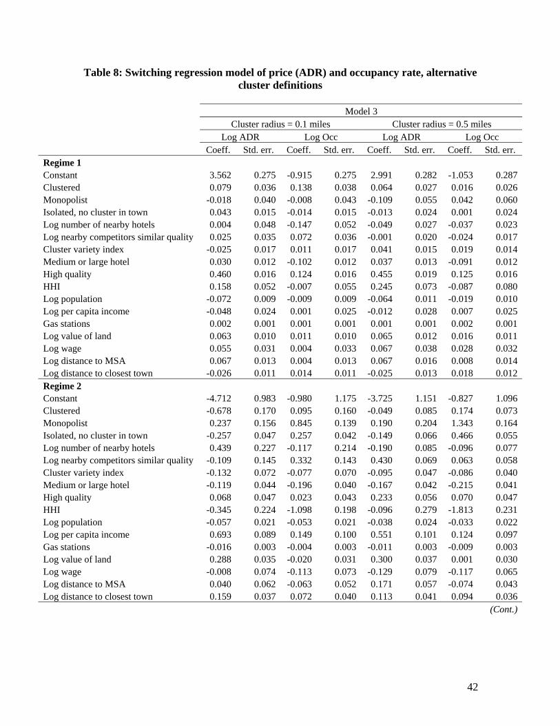
42

Table 8: Switching regression model of price (ADR) and occupancy rate, alternative cluster definitions

Model 3 Cluster radius = 0.1 miles Cluster radius = 0.5 miles Log ADR Log Occ Log ADR Log Occ Coeff. Std. err. Coeff. Std. err. Coeff. Std. err. Coeff. Std. err. Regime 1 Constant 3.562 0.275 -0.915 0.275 2.991 0.282 -1.053 0.287 Clustered 0.079 0.036 0.138 0.038 0.064 0.027 0.016 0.026 Monopolist -0.018 0.040 -0.008 0.043 -0.109 0.055 0.042 0.060 Isolated, no cluster in town 0.043 0.015 -0.014 0.015 -0.013 0.024 0.001 0.024 Log number of nearby hotels 0.004 0.048 -0.147 0.052 -0.049 0.027 -0.037 0.023 Log nearby competitors similar quality 0.025 0.035 0.072 0.036 -0.001 0.020 -0.024 0.017 Cluster variety index -0.025 0.017 0.011 0.017 0.041 0.015 0.019 0.014 Medium or large hotel 0.030 0.012 -0.102 0.012 0.037 0.013 -0.091 0.012 High quality 0.460 0.016 0.124 0.016 0.455 0.019 0.125 0.016 HHI 0.158 0.052 -0.007 0.055 0.245 0.073 -0.087 0.080 Log population -0.072 0.009 -0.009 0.009 -0.064 0.011 -0.019 0.010 Log per capita income -0.048 0.024 0.001 0.025 -0.012 0.028 0.007 0.025 Gas stations 0.002 0.001 0.001 0.001 0.001 0.001 0.002 0.001 Log value of land 0.063 0.010 0.011 0.010 0.065 0.012 0.016 0.011 Log wage 0.055 0.031 0.004 0.033 0.067 0.038 0.028 0.032 Log distance to MSA 0.067 0.013 0.004 0.013 0.067 0.016 0.008 0.014 Log distance to closest town -0.026 0.011 0.014 0.011 -0.025 0.013 0.018 0.012 Regime 2 Constant -4.712 0.983 -0.980 1.175 -3.725 1.151 -0.827 1.096 Clustered -0.678 0.170 0.095 0.160 -0.049 0.085 0.174 0.073 Monopolist 0.237 0.156 0.845 0.139 0.190 0.204 1.343 0.164 Isolated, no cluster in town -0.257 0.047 0.257 0.042 -0.149 0.066 0.466 0.055 Log number of nearby hotels 0.439 0.227 -0.117 0.214 -0.190 0.085 -0.096 0.077 Log nearby competitors similar quality -0.109 0.145 0.332 0.143 0.430 0.069 0.063 0.058 Cluster variety index -0.132 0.072 -0.077 0.070 -0.095 0.047 -0.086 0.040 Medium or large hotel -0.119 0.044 -0.196 0.040 -0.167 0.042 -0.215 0.041 High quality 0.068 0.047 0.023 0.043 0.233 0.056 0.070 0.047 HHI -0.345 0.224 -1.098 0.198 -0.096 0.279 -1.813 0.231 Log population -0.057 0.021 -0.053 0.021 -0.038 0.024 -0.033 0.022 Log per capita income 0.693 0.089 0.149 0.100 0.551 0.101 0.124 0.097 Gas stations -0.016 0.003 -0.004 0.003 -0.011 0.003 -0.009 0.003 Log value of land 0.288 0.035 -0.020 0.031 0.300 0.037 0.001 0.030 Log wage -0.008 0.074 -0.113 0.073 -0.129 0.079 -0.117 0.065 Log distance to MSA 0.040 0.062 -0.063 0.052 0.171 0.057 -0.074 0.043 Log distance to closest town 0.159 0.037 0.072 0.040 0.113 0.041 0.094 0.036 (Cont.)

43

Model 3 Cluster radius = 0.1 miles Cluster radius = 0.5 miles Coeff. Std. err. Coeff. Std. err. Probability of Regime 1

Constant 0.962 0.091 0.489 0.106

Clustered 1.060 0.377 1.462 0.176

Monopolist 0.476 0.126 0.818 0.140

Isolated, no cluster in town -0.227 0.109 -0.213 0.135

Log number of nearby hotels -0.592 0.348 -0.449 0.101

High season -0.155 0.072 -0.119 0.077

Medium or large hotel 1.438 0.117 1.463 0.114

If Central Texas or Metroplex -0.882 0.095 -0.814 0.103

If South Texas or Gulf Coast -1.045 0.102 -1.064 0.106

σε1 0.228 0.003 0.228 0.004

σu1 0.236 0.004 0.234 0.003

ρ1 0.372 0.006 0.387 0.006

σε2 0.454 0.012 0.463 0.010

σu2 0.437 0.009 0.436 0.007

ρ2 0.253 0.014 0.202 0.014 # observations 9,148 9,148 Log likelihood -5,154.1 -5,102.5 Note: All models include major top-chain, regional and time-period dummies. The top chains are Best Western, Best Value, Comfort, Days, Econolodge, Holiday, Motel 6, Super 8, and Ramada. A hotel is considered clustered if it has a nearby competitor in town in a radius of 0.1 (0.5) miles. Number of nearby hotels corresponds to the number of hotels that are within a radius of 0.1 (0.5) miles from the hotel in the observation (the same for the number of nearby competitors of similar quality). The variety index is calculated based on hotel quality (1-4 diamonds). Metroplex is located to the north of Central Texas. HHI is treated as endogenous. Variance of correlation coefficient obtained using the delta method.

44

Table 9: Switching regression model of price (ADR) and occupancy rate, alternative specification (Cluster radius=0.2 miles)

Model 3 Log ADR Log Occ Coeff. Std. err. Coeff. Std. err. Regime 1 Constant 1.632 0.477 -0.950 0.464 Clustered 0.068 0.035 0.083 0.027 Monopolist 0.014 0.058 0.021 0.049 Isolated, no cluster in town 0.065 0.020 0.007 0.018 Log number of nearby hotels 0.069 0.040 -0.089 0.030 Log nearby competitors similar quality -0.064 0.028 0.030 0.022 Cluster variety index -0.045 0.019 0.014 0.018 Medium or large hotel 0.033 0.013 -0.094 0.012 High quality 0.472 0.021 0.122 0.016 HHI 0.142 0.076 -0.043 0.064 Log population -0.074 0.010 -0.012 0.009 Log per capita income -0.033 0.031 0.005 0.027 Gas stations 0.002 0.001 0.001 0.001 Log value of land 0.065 0.014 0.007 0.012 Log wage 0.070 0.039 0.038 0.031 Log distance to MSA 0.068 0.017 0.011 0.014 Log distance to closest town -0.030 0.013 0.017 0.011 Regime 2 Constant -2.972 1.254 -0.575 1.044 Clustered -0.777 0.112 0.072 0.095 Monopolist 0.286 0.187 0.895 0.139 Isolated, no cluster in town -0.160 0.054 0.268 0.042 Log number of nearby hotels 0.666 0.143 0.006 0.122 Log nearby competitors similar quality -0.116 0.100 0.092 0.084 Cluster variety index -0.172 0.058 -0.111 0.051 Medium or large hotel -0.153 0.048 -0.192 0.042 High quality 0.074 0.053 0.045 0.045 HHI -0.325 0.258 -1.169 0.201 Log population -0.042 0.026 -0.054 0.020 Log per capita income 0.634 0.105 0.148 0.094 Gas stations -0.015 0.003 -0.005 0.003 Log value of land 0.295 0.038 -0.009 0.031 Log wage -0.059 0.089 -0.135 0.070 Log distance to MSA 0.004 0.061 -0.059 0.047 Log distance to closest town 0.133 0.048 0.052 0.041 (Cont.)

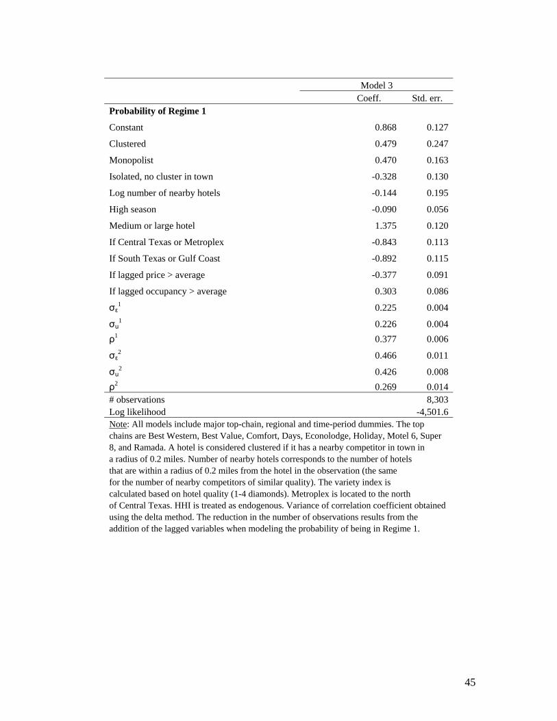
45

Model 3 Coeff. Std. err. Probability of Regime 1

Constant 0.868 0.127

Clustered 0.479 0.247

Monopolist 0.470 0.163

Isolated, no cluster in town -0.328 0.130

Log number of nearby hotels -0.144 0.195

High season -0.090 0.056

Medium or large hotel 1.375 0.120

If Central Texas or Metroplex -0.843 0.113

If South Texas or Gulf Coast -0.892 0.115

If lagged price > average -0.377 0.091

If lagged occupancy > average 0.303 0.086

σε1 0.225 0.004

σu1 0.226 0.004

ρ1 0.377 0.006

σε2 0.466 0.011

σu2 0.426 0.008

ρ2 0.269 0.014 # observations 8,303 Log likelihood -4,501.6 Note: All models include major top-chain, regional and time-period dummies. The top chains are Best Western, Best Value, Comfort, Days, Econolodge, Holiday, Motel 6, Super 8, and Ramada. A hotel is considered clustered if it has a nearby competitor in town in a radius of 0.2 miles. Number of nearby hotels corresponds to the number of hotels that are within a radius of 0.2 miles from the hotel in the observation (the same for the number of nearby competitors of similar quality). The variety index is calculated based on hotel quality (1-4 diamonds). Metroplex is located to the north of Central Texas. HHI is treated as endogenous. Variance of correlation coefficient obtained using the delta method. The reduction in the number of observations results from the addition of the lagged variables when modeling the probability of being in Regime 1.

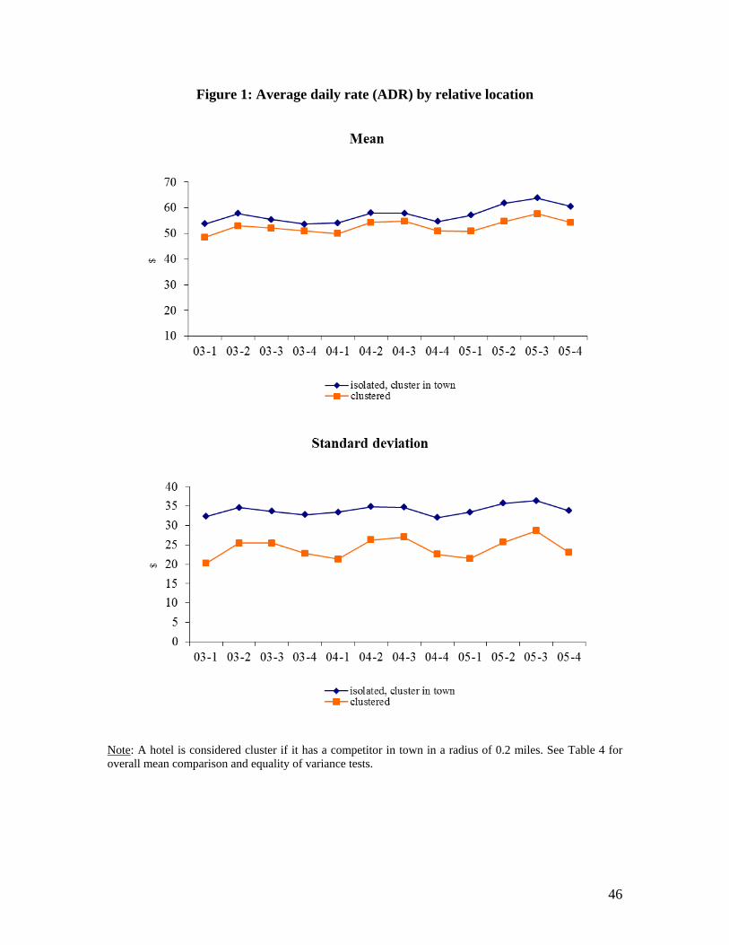
46

Figure 1: Average daily rate (ADR) by relative location

Note: A hotel is considered cluster if it has a competitor in town in a radius of 0.2 miles. See Table 4 for overall mean comparison and equality of variance tests.

47

Figure 2: Occupancy rate by relative location

Note: A hotel is considered cluster if it has a competitor in town in a radius of 0.2 miles. See Table 4 for overall mean comparison and equality of variance tests.

48

Figure 3: Probability of colluding, conditional on being clustered

0.40

0.50

0.60

0.70

0.80

0.90

1.00

1 2 3 4 5 6

Prob

abili

ty o

f col

ludi

ng

# additional hotels in cluster

Small hotel, low season Small hotel, high season

Medium and large hotel, low season Medium and large hotel, high season

49

Figure 4: Probability of colluding, conditional on being clustered (by cluster definition)

0.40

0.50

0.60

0.70

0.80

0.90

1.00

1 2 3 4 5 6

Prob

abili

ty o

f col

ludi

ng

# additional hotels in cluster

cluster radius = 0.2 miles cluster radius = 0.1 miles cluster radius = 0.5 miles

Note: Probabilities based on a small hotel and low season.

50

Table A.1: Texas Hotel Performance Factbook – Description of variables

Room counts Are checked annually in chain directories and the Texas American Automobile Association (AAA) tour book. These properties account for approximately 80% of the state revenues. Properties are also checked by calling census and physical inspection by Source Strategies Inc. (SSI). For independent properties too small to be listed, the room counts reported to the Texas state government are used (unless they appear unreasonable). As a result, “Chains” room counts are very close to actual, while independent room counts could be slightly overstated.

Average Daily Rates (ADR) Obtained from financial reports, appraisers, private SSI surveys, chain

and AAA directories, and another reliable industry database.

Occupancy rate Is calculated from room nights sold and room nights available. All

occupancy figures represent fully-weighted averages. Room nights sold are obtained by dividing gross room revenues reported to the State of Texas Comptroller by ADR. Room nights available are calculated from room counts times the number of days in the period.

“Chains” Are defined as one of the "Top 50+" brands determined and tracked by

SSI. These brands may vary across time. Our sample includes, among others, Americas Best Value, Best Western, Budget Host, Comfort, Days, Econo Lodge, Hampton, Holiday, La Quinta, Motel 6, Ramada, and Super 8.

Note: According to SSI, on an overall basis the changes in ADR reported are within a few tenths of one-percent of Smith Travel's “Lodging Outlook”. Smith Travel Research (STR) is a private research firm that gets full financial reports of hotel/motel properties, accounting for 80% of the market, but it only publishes aggregate results.

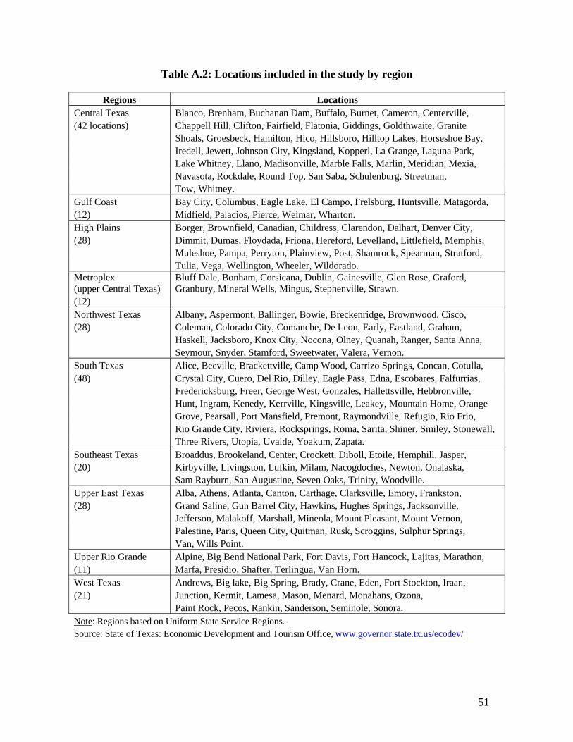
51

Table A.2: Locations included in the study by region

Regions Locations Central Texas Blanco, Brenham, Buchanan Dam, Buffalo, Burnet, Cameron, Centerville, (42 locations) Chappell Hill, Clifton, Fairfield, Flatonia, Giddings, Goldthwaite, Granite Shoals, Groesbeck, Hamilton, Hico, Hillsboro, Hilltop Lakes, Horseshoe Bay, Iredell, Jewett, Johnson City, Kingsland, Kopperl, La Grange, Laguna Park, Lake Whitney, Llano, Madisonville, Marble Falls, Marlin, Meridian, Mexia, Navasota, Rockdale, Round Top, San Saba, Schulenburg, Streetman, Tow, Whitney. Gulf Coast Bay City, Columbus, Eagle Lake, El Campo, Frelsburg, Huntsville, Matagorda, (12) Midfield, Palacios, Pierce, Weimar, Wharton. High Plains Borger, Brownfield, Canadian, Childress, Clarendon, Dalhart, Denver City, (28) Dimmit, Dumas, Floydada, Friona, Hereford, Levelland, Littlefield, Memphis, Muleshoe, Pampa, Perryton, Plainview, Post, Shamrock, Spearman, Stratford, Tulia, Vega, Wellington, Wheeler, Wildorado. Metroplex (upper Central Texas) (12)

Bluff Dale, Bonham, Corsicana, Dublin, Gainesville, Glen Rose, Graford, Granbury, Mineral Wells, Mingus, Stephenville, Strawn.

Northwest Texas Albany, Aspermont, Ballinger, Bowie, Breckenridge, Brownwood, Cisco, (28) Coleman, Colorado City, Comanche, De Leon, Early, Eastland, Graham, Haskell, Jacksboro, Knox City, Nocona, Olney, Quanah, Ranger, Santa Anna, Seymour, Snyder, Stamford, Sweetwater, Valera, Vernon. South Texas Alice, Beeville, Brackettville, Camp Wood, Carrizo Springs, Concan, Cotulla, (48) Crystal City, Cuero, Del Rio, Dilley, Eagle Pass, Edna, Escobares, Falfurrias, Fredericksburg, Freer, George West, Gonzales, Hallettsville, Hebbronville, Hunt, Ingram, Kenedy, Kerrville, Kingsville, Leakey, Mountain Home, Orange Grove, Pearsall, Port Mansfield, Premont, Raymondville, Refugio, Rio Frio, Rio Grande City, Riviera, Rocksprings, Roma, Sarita, Shiner, Smiley, Stonewall, Three Rivers, Utopia, Uvalde, Yoakum, Zapata. Southeast Texas Broaddus, Brookeland, Center, Crockett, Diboll, Etoile, Hemphill, Jasper, (20) Kirbyville, Livingston, Lufkin, Milam, Nacogdoches, Newton, Onalaska, Sam Rayburn, San Augustine, Seven Oaks, Trinity, Woodville. Upper East Texas Alba, Athens, Atlanta, Canton, Carthage, Clarksville, Emory, Frankston, (28) Grand Saline, Gun Barrel City, Hawkins, Hughes Springs, Jacksonville, Jefferson, Malakoff, Marshall, Mineola, Mount Pleasant, Mount Vernon, Palestine, Paris, Queen City, Quitman, Rusk, Scroggins, Sulphur Springs, Van, Wills Point. Upper Rio Grande Alpine, Big Bend National Park, Fort Davis, Fort Hancock, Lajitas, Marathon, (11) Marfa, Presidio, Shafter, Terlingua, Van Horn. West Texas Andrews, Big lake, Big Spring, Brady, Crane, Eden, Fort Stockton, Iraan, (21) Junction, Kermit, Lamesa, Mason, Menard, Monahans, Ozona, Paint Rock, Pecos, Rankin, Sanderson, Seminole, Sonora. Note: Regions based on Uniform State Service Regions. Source: State of Texas: Economic Development and Tourism Office, www.governor.state.tx.us/ecodev/

52

Table A.3: Sources of information consulted to construct market controls

Source Variable Texas State Data Center and Office of Population the State Demographer Annual population at the county level. Texas Population Estimates Program http://txsdc.utsa.edu/tpepp/txpopest.php Bureau of Economic Analysis Per capita income http://bea.gov/bea/regional/reis Annual per capita personal income at the county level. Google Maps Gas stations www.google.com Number of gas stations at each location. Real Estate Center at Texas A&M University Value of land www.recenter.tamu.edu/data/agp Median per-acre value of rural land per year at the land market area. Bureau of Labor Statistics Wage www.bls.gov/data/home.htm Average weekly wage on leisure and hospitality per quarter at the county level. Texas Comptroller of Public Accounts Distance to MSA Texas Mileage Guide Mileage between location and nearest MSA. www.window.state.tx.us/comptrol/texastra.html MapQuest (for missing locations) www.mapquest.com Texas Tourism Travel Industry website Regional dummies based on Uniform State Economic Impact of Travel 2005 Service Regions. www.travel.state.tx.us/EconomicImpact.aspx

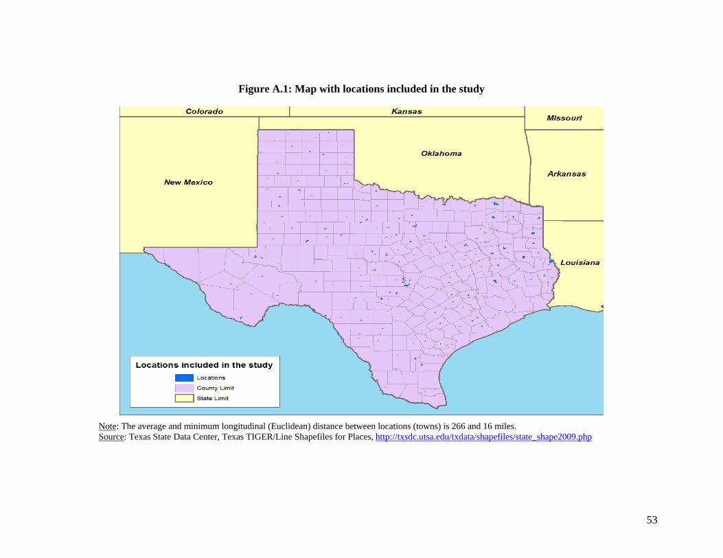
53

Figure A.1: Map with locations included in the study

Note: The average and minimum longitudinal (Euclidean) distance between locations (towns) is 266 and 16 miles. Source: Texas State Data Center, Texas TIGER/Line Shapefiles for Places, http://txsdc.utsa.edu/txdata/shapefiles/state_shape2009.php