MAJORANA FERMION IN TOPOLOGICAL

SUPERCONDUCTOR AND MOTT-SUPERFLUID

TRANSITION IN CIRCUIT-QED SYSTEM

JIA-BIN YOU

NATIONAL UNIVERSITY OF SINGAPORE

2015

MAJORANA FERMION IN TOPOLOGICAL

SUPERCONDUCTOR AND MOTT-SUPERFLUID

TRANSITION IN CIRCUIT-QED SYSTEM

JIA-BIN YOU

(M.Sc., XMU)

CENTRE FOR QUANTUM TECHNOLOGIES

NATIONAL UNIVERSITY OF SINGAPORE

A THESIS SUBMITTED FOR THE DEGREE OF

DOCTOR OF PHILOSOPHY

2015

Declaration

I hereby declare that the thesis is my original

work and it has been written by me in its

entirety. I have duly acknowledged all the

sources of information which have been used

in the thesis.

This thesis has also not been submitted for

any degree in any university previously.

Jia-Bin You

September 1, 2015

i

Acknowledgements

I would like to thank my colleagues, friends, and family for their continued

support throughout my PhD candidature. Especially, I would like to express

my deepest appreciation to my supervisor, Professor Oh Choo Hiap, for giving

me the chance to live and study in this beautiful country, and for all his help

and guidance during the completion of this research. I also thank Professor

Vlatko Vedral for his collaborations and useful advice as my co-supervisor at

Centre for Quantum Technologies. Additionally, I would like to acknowledge

the members of my Thesis Advisory Committee, Professor Lai Choy Heng,

Vlatko Vedral and Phil Chan, for their academic advice during my qualifying

exam. The works in this thesis have been funded by the CQT Scholarship, and

the National Research Foundation and Ministry of Education of Singapore.

I have benefited tremendously from discussing physics with other col-

leagues and friends at Centre for Quantum Technologies and Department

of Physics. Interactions with them are always enlightening and fruitful. A

very partial list includes Chen Qing, Cui Jian, Deng Donglin, Feng Xunli,

Guo Chu, Huang Jinsong, Lee Hsin-Han, Li Ying, Lu Xiaoming, Luo Ziyu,

Luo Yongzheng, Mei Feng, Nie Wei, Peng Jiebin, Qian Jun, Qiao Youming,

Shao Xiaoqiang, Sun Chunfang, Tang Weidong, Tian Guojing, Tong Qingjun,

Wang Hui, Wang Yibo, Wang Zhuo, Wu Chunfeng, Yang Wanli, Yao Penghui,

Yu Liwei, Yu Sixia, Zeng Shengwei, Zhang Yixing, Zhu Huangjun. I also wish

to thank them and many others for enriching my graduate life.

ii

Contents

Contents iii

Abstract v

1 Introduction 1

I Majorana fermion in topological superconductor 5

2 Topological quantum phase transition in spin-singlet superconductor 6

2.1 Introduction . . . . . . . . . . . . . . . . . . . . . . . . . . . . . . . . . . 6

2.2 Theoretical model for the spin-singlet topological superconductor . . . . 8

2.3 s-wave Rashba superconductor . . . . . . . . . . . . . . . . . . . . . . . . 9

2.4 s-wave Dresselhaus superconductor . . . . . . . . . . . . . . . . . . . . . 12

2.5 Topological properties of the spin-singlet superconductor . . . . . . . . . 18

2.5.1 symmetries of the BdG Hamiltonian . . . . . . . . . . . . . . . . 18

2.5.2 topological invariants of the BdG Hamiltonian . . . . . . . . . . . 19

2.5.3 phase diagrams of the BdG Hamiltonian . . . . . . . . . . . . . . 24

2.5.4 Majorana bound states at the edge of the BdG Hamiltonian . . . 25

3 Majorana transport in superconducting nanowire with Rashba and Dres-

selhaus spin-orbit couplings 31

3.1 Introduction . . . . . . . . . . . . . . . . . . . . . . . . . . . . . . . . . . 31

3.2 Model . . . . . . . . . . . . . . . . . . . . . . . . . . . . . . . . . . . . . 33

3.3 NEGF method for the Majorana current . . . . . . . . . . . . . . . . . . 36

3.3.1 general formula . . . . . . . . . . . . . . . . . . . . . . . . . . . . 36

3.3.2 dc current response . . . . . . . . . . . . . . . . . . . . . . . . . . 40

3.3.3 ac current response . . . . . . . . . . . . . . . . . . . . . . . . . . 43

iii

3.4 Interaction and disorder effects on the Majorana transport . . . . . . . . 43

3.4.1 brief introduction of bosonization . . . . . . . . . . . . . . . . . . 46

3.4.1.1 left and right movers representation . . . . . . . . . . . . 46

3.4.1.2 bosonization of the Majorana nanowire . . . . . . . . . . 51

3.4.2 influence on the Majorana transport . . . . . . . . . . . . . . . . 52

II Mott-superfluid transition in hybrid circuit-QED system 55

4 Phase transition of light in circuit-QED lattices coupled to nitrogen-

vacancy centers in diamond 56

4.1 Introduction . . . . . . . . . . . . . . . . . . . . . . . . . . . . . . . . . . 56

4.2 Model . . . . . . . . . . . . . . . . . . . . . . . . . . . . . . . . . . . . . 57

4.3 Mott-superfluid transition . . . . . . . . . . . . . . . . . . . . . . . . . . 62

4.4 Dissipative effects . . . . . . . . . . . . . . . . . . . . . . . . . . . . . . . 67

4.5 Experimental feasibility . . . . . . . . . . . . . . . . . . . . . . . . . . . 68

5 Summary and outlook 70

A Edge spectra of topological superconductor with mixed spin-singlet

pairings 72

B Keldysh non-equilibrium Green function 76

C Green function and self-energy for Majorana nanowire 80

D Useful expressions for the free Green functions 84

E Fermion-boson correspondence in one dimension 86

F Normal-ordered density operator 90

G Replica method 92

H Renormalization analysis of correlation function 94

I Quantum trajectory method 99

Bibliography 101

iv

Abstract

The thesis contains two parts. Part I comprises two chapters and concerns

Majorana fermion in topological superconductors. Part II is a study of Mott-

superfluid transition in hybrid circuit-QED system.

In Part I, we study the Majorana fermion and its transport in the topo-

logical superconductors. In Chapter 2, we investigate the edge states and

the vortex core states in the spin-singlet (s-wave and d-wave) superconduc-

tor with Rashba and Dresselhaus (110) spin-orbit couplings. We show that

there are several topological invariants in the Bogoliubov-de Gennes (BdG)

Hamiltonian by symmetry analysis. The edge spectrum of the superconduc-

tors is either Dirac cone or flat band which supports the emergence of the

Majorana fermion. For the Majorana flat bands, an edge index, namely the

Pfaffian invariant P(ky) or the winding number W(ky), is needed to make

them topologically stable. In Chapter 3, we use Keldysh non-equilibrium

Green function method to study the two-lead tunneling in the superconduct-

ing nanowire with Rashba and Dresselhaus spin-orbit couplings. The dc and

ac current responses of the nanowire are considered. Interestingly, due to the

exotic property of Majorana fermion, there exists a hole transmission channel

which makes the currents asymmetric at the left and right leads. We em-

ploy the bosonization and renormalization group method to study the phase

diagram of the wire with Coulomb interaction and disorder and discuss the

impact on the transport property.

In Part II (Chapter 4), we propose a hybrid quantum architecture for

engineering a photonic Mott insulator-superfluid phase transition in a two-

dimensional square lattice of a superconducting transmission line resonator

coupled to a single nitrogen-vacancy center encircled by a persistent current

qubit. The phase diagrams in the case of real-value and complex-value pho-

tonic hopping are obtained using the mean-field approach. Also, the quantum

jump technique is employed to describe the phase diagram when the dissipa-

tive effects are considered.

v

Publications

1. Jia-Bin You, Xiao-Qiang Shao, Qing-Jun Tong, A. H. Chan, C. H. Oh,

and Vlatko Vedral, Majorana transport in superconducting nanowire with

Rashba and Dresselhaus spin-orbit couplings. Journal of Physics: Con-

densed Matter 27, 225302 (2015).

2. Jia-Bin You, W. L. Yang, Zhen-Yu Xu, A. H. Chan, and C. H. Oh, Phase

transition of light in circuit-QED lattices coupled to nitrogen-vacancy

centers in diamond. Physical Review B 90, 195112 (2014).

3. Jia-Bin You, A. H. Chan, C. H. Oh and Vlatko Vedral, Topological

quantum phase transitions in the spin-singlet superconductor with Rashba

and Dresselhaus (110) spin-orbit couplings. Annals of Physics 349, 189

(2014).

4. Jia-Bin You, C. H. Oh and Vlatko Vedral, Majorana fermions in s-

wave noncentrosymmetric superconductor with Dresselhaus (110) spin-

orbit coupling. Physical Review B 87, 054501 (2013).

vi

Chapter 1

Introduction

The thesis contains two parts. The first part (Chapter 2 and 3) concerns Majo-

rana fermions in two dimensional and one dimensional topological superconductors. The

second part (Chapter 4) concerns Mott insulator-superfluid transition in hybrid circuit

quantum electrodynamics (QED) system.

In Chapter 2, we study the topological phase in the Rashba and Dresselhaus spin-

singlet superconductors. It is amazing that the various phases in our world can be

understood systematically by Landau symmetry breaking theory. However, in the last

several decades, it was discovered that there are even more interesting phases that are

beyond Landau symmetry breaking theory [163]. One of these new phases is topological

superconductor which is new state of quantum matter that is characterized by topological

order such as Chern number or Pfaffian invariant [3; 4; 14; 33; 45; 66; 79; 88; 125; 131;

132; 134; 139; 146; 166]. The topologically ordered phases have a full superconducting

gap in the bulk and localized states in the edge or surface. Interestingly, these localized

edge states can host Majorana fermions which are neutral particles that are their own

antiparticles [45; 104; 119; 125; 131]. The solid-state Majorana fermions can be used for a

topological quantum computer, in which the non-Abelian exchange statistics of the Majo-

rana fermions are used to process quantum information nonlocally, evading error-inducing

local perturbations [29; 40; 79; 113]. In this Chapter, we investigate the edge states and

the vortex core states in the s-wave superconductor with Rashba and Dresselhaus (110)

spin-orbit couplings. Particularly, we demonstrate that there exists a semimetal phase

characterized by the dispersionless Majorana flat bands in the phase diagram of the s-

wave Dresselhaus superconductor which supports the emergence of Majorana fermions.

We then extend our study to the spin-singlet (s-wave and d-wave) superconductor with

Rashba and Dresselhaus (110) spin-orbit couplings. We show that there are several topo-

1

logical invariants in the Bogoliubov-de Gennes (BdG) Hamiltonian by symmetry analysis.

The Pfaffian invariant P for the particle-hole symmetry can be used to demonstrate all

the possible phase diagrams of the BdG Hamiltonian. We find that the edge spectrum

is either Dirac cone or flat band which supports the emergence of the Majorana fermion.

For the Majorana flat bands, an edge index, namely the Pfaffian invariant P(ky) or the

winding number W(ky), is needed to make them topologically stable. These edge indices

can also be used in determining the location of the Majorana flat bands. The main results

of this Chapter were published in our following papers:

• Jia-Bin You, C. H. Oh and Vlatko Vedral, Majorana fermions in s-wave noncen-

trosymmetric superconductor with Dresselhaus (110) spin-orbit coupling. Physical

Review B 87, 054501 (2013).

• Jia-Bin You, A. H. Chan, C. H. Oh and Vlatko Vedral, Topological quantum phase

transitions in the spin-singlet superconductor with Rashba and Dresselhaus (110)

spin-orbit couplings. Annals of Physics 349, 189 (2014).

In Chapter 3, we use Keldysh non-equilibrium Green function method to study two-

lead tunneling in superconducting nanowire with Rashba and Dresselhaus spin-orbit cou-

plings [12; 30; 32; 36; 42; 71; 86; 100; 106; 173; 175]. The tunneling spectroscopy is

a key probe for detecting Majorana fermions [40; 42; 90; 122; 135; 142]. The Majo-

rana fermions would manifest as a conductance peak at zero voltage as long as they

are spatially separated from each other. Indeed, numerous experimental results have

reported zero-bias conductance peak in devices inspired by the theoretical proposals

[19; 23; 27; 28; 31; 40; 91; 109]. In this Chapter, we first study the zero-bias dc con-

ductance peak appearing in our two-lead setup. Interestingly, due to the exotic property

of Majorana fermion, there exists a hole transmission channel which makes the currents

asymmetric at the left and right leads. The ac current response mediated by Majorana

fermion is also studied in the thesis. To discuss the impacts of Coulomb interaction and

disorder on the transport property of Majorana nanowire, we use the renormalization

group method to study the phase diagram of the wire. It is found that there is a topo-

logical phase transition under the interplay of superconductivity and disorder. We find

that the Majorana transport is preserved in the superconducting-dominated topologi-

cal phase and destroyed in the disorder-dominated non-topological insulator phase. The

main results of this Chapter are from the following paper:

• Jia-Bin You, Xiao-Qiang Shao, Qing-Jun Tong, A. H. Chan, C. H. Oh, and Vlatko

Vedral, Majorana transport in superconducting nanowire with Rashba and Dres-

2

selhaus spin-orbit couplings. Journal of Physics: Condensed Matter 27, 225302

(2015).

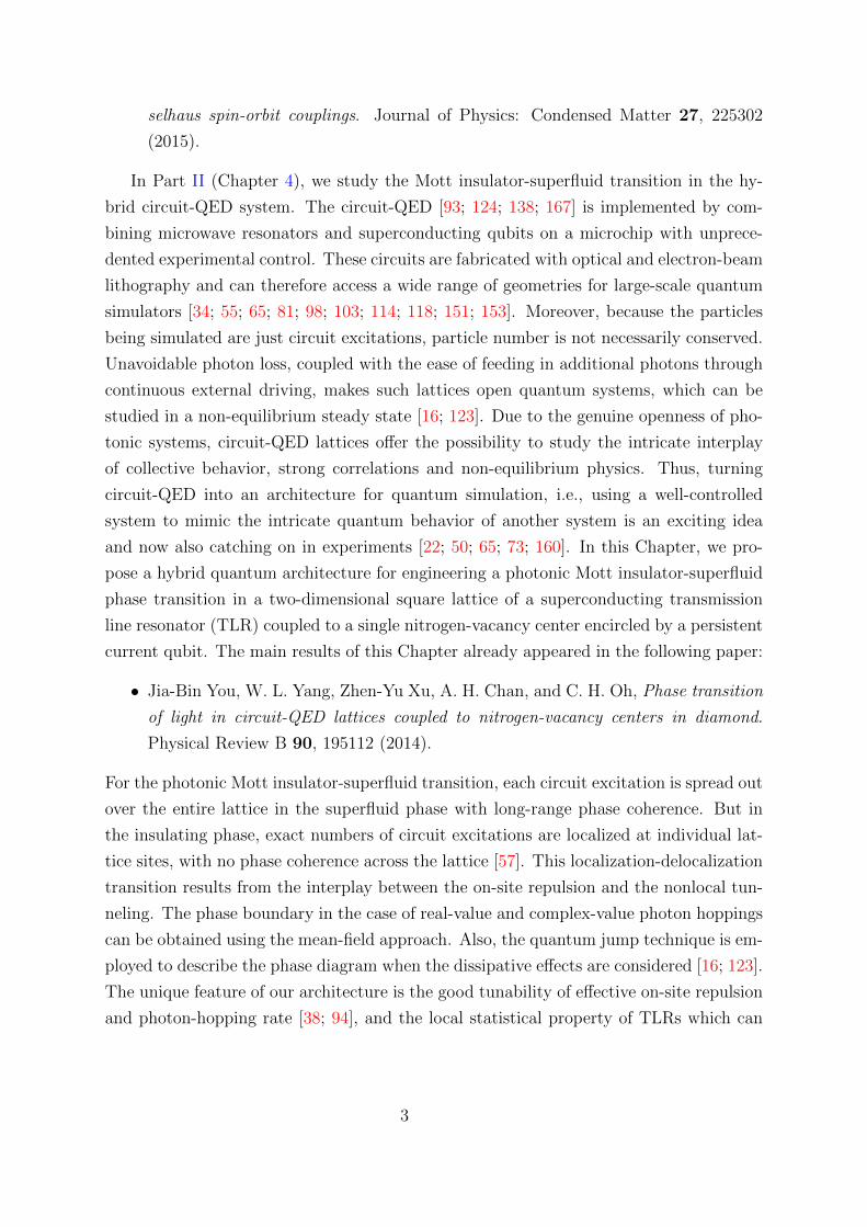
In Part II (Chapter 4), we study the Mott insulator-superfluid transition in the hy-

brid circuit-QED system. The circuit-QED [93; 124; 138; 167] is implemented by com-

bining microwave resonators and superconducting qubits on a microchip with unprece-

dented experimental control. These circuits are fabricated with optical and electron-beam

lithography and can therefore access a wide range of geometries for large-scale quantum

simulators [34; 55; 65; 81; 98; 103; 114; 118; 151; 153]. Moreover, because the particles

being simulated are just circuit excitations, particle number is not necessarily conserved.

Unavoidable photon loss, coupled with the ease of feeding in additional photons through

continuous external driving, makes such lattices open quantum systems, which can be

studied in a non-equilibrium steady state [16; 123]. Due to the genuine openness of pho-

tonic systems, circuit-QED lattices offer the possibility to study the intricate interplay

of collective behavior, strong correlations and non-equilibrium physics. Thus, turning

circuit-QED into an architecture for quantum simulation, i.e., using a well-controlled

system to mimic the intricate quantum behavior of another system is an exciting idea

and now also catching on in experiments [22; 50; 65; 73; 160]. In this Chapter, we pro-

pose a hybrid quantum architecture for engineering a photonic Mott insulator-superfluid

phase transition in a two-dimensional square lattice of a superconducting transmission

line resonator (TLR) coupled to a single nitrogen-vacancy center encircled by a persistent

current qubit. The main results of this Chapter already appeared in the following paper:

• Jia-Bin You, W. L. Yang, Zhen-Yu Xu, A. H. Chan, and C. H. Oh, Phase transition

of light in circuit-QED lattices coupled to nitrogen-vacancy centers in diamond.

Physical Review B 90, 195112 (2014).

For the photonic Mott insulator-superfluid transition, each circuit excitation is spread out

over the entire lattice in the superfluid phase with long-range phase coherence. But in

the insulating phase, exact numbers of circuit excitations are localized at individual lat-

tice sites, with no phase coherence across the lattice [57]. This localization-delocalization

transition results from the interplay between the on-site repulsion and the nonlocal tun-

neling. The phase boundary in the case of real-value and complex-value photon hoppings

can be obtained using the mean-field approach. Also, the quantum jump technique is em-

ployed to describe the phase diagram when the dissipative effects are considered [16; 123].

The unique feature of our architecture is the good tunability of effective on-site repulsion

and photon-hopping rate [38; 94], and the local statistical property of TLRs which can

3

be analyzed readily using present microwave techniques [43; 74; 92; 141; 144; 149]. Our

work gives new perspectives in quantum simulation of condensed-matter and many-body

physics using a hybrid circuit-QED system. The experimental challenges are realizable

using current technologies.

4

Part I

Majorana fermion in topological

superconductor

5

Chapter 2

Topological quantum phase

transition in spin-singlet

superconductor

2.1 Introduction

Topological phase of condensed matter systems refers to a quantum many-body state

with nontrivial topology in the momentum or coordinate space [3; 8; 45; 46; 58; 66;

76; 77; 83; 119; 125; 129; 131; 134; 147; 148; 158]. Recent newly discovered topological

superconductor (TSC) has spawned considerable interests since this kind of topological

phase supports the emergence of Majorana fermion (MF) [45; 104; 119; 125; 131] which

is a promising candidate for the fault-tolerant topological quantum computation [80].

There are several proposals for hosting MFs in TSC, for example, chiral p-wave super-

conductor [125], Cu-doped topological insulator Bi2Se3 [66], superconducting proximity

devices [3; 4; 45; 79; 88; 134] and noncentrosymmetric superconductor such as CePt3Si

and Li2PdxPt3−xB [14; 33; 131; 132; 139; 146; 166]. The signatures of MFs have also

been reported in the transport measurement of superconducting InSb nanowire [28; 109],

CuxBi2Se3 [7; 127] and topological insulator Josephson junction [164].

There are two kinds of gapless edge states in the topological superconductor. One is

a Dirac cone, the other is a flat band, namely, dispersionless zero-energy state [14; 33; 88;

132; 139; 166; 170]. The Dirac cone can be found in the fully gapped topological super-

conductors when the Chern number of the occupied energy bands is nonzero. However,

the flat band can appear in the gapless topological superconductors which, apart from

6

the particle-hole symmetry, have some extra symmetries in the Hamiltonian. Such flat

bands are known to occur at the zigzag and bearded edge in graphene [110], in the non-

centrosymmetric superconductor [14; 132; 139] and in other systems with topologically

stable Dirac points [159].

In Sec. 2.2, we give a model for the spin-singlet superconductor with Rashba and

Dresselhaus (110) spin-orbit (SO) couplings. In Sec. 2.3, we briefly discuss the topological

number and the edge spectrum of the s-wave Rashba superconductor. In Sec. 2.4, we

focus on the topological phase and the Majorana fermion at the edge and in the vortex

core of the s-wave Dresselhaus superconductor. Interestingly, we find that there is a

novel semimetal phase in the Dresselhaus superconductor, where the energy gap closes

and different kinds of flat band emerge. We demonstrate that these flat bands support

the emergence of MFs analytically and numerically. It is known that the Chern number

is not a well-defined topological invariant in the gapless energy-band structure, however,

we find that the topologically different semimetal phases can still be distinguished by the

Pfaffian invariant of the particle-hole symmetric Hamiltonian.

In Sec. 2.5, we generalize our study to the spin-singlet superconductor with the

Rashba and Dresselhaus (110) spin-orbit couplings. We focus on the Hamiltonian with

spin-orbit coupling of Dresselhaus (110) type which is a gapless topological system con-

taining two kinds of edge states mentioned above. For the topological numbers of the

Hamiltonian of the spin-singlet superconductor, the Bogoliubov-de Gennes (BdG) Hamil-

tonian of the superconductor is particle-hole symmetric so that we can associate a Pfaffian

invariant P with it as a topological invariant of the system. In particular, the Pfaffian in-

variant P can be used in distinguishing the topologically nontrivial phase from the trivial

one and we find all the possible phase diagrams of the BdG Hamiltonian in Sec. 2.5.3.

The nontrivial topological phase in this BdG Hamiltonian is Majorana type which can

be exploited for implementing the fault-tolerant topological quantum computing schemes

[79; 113]. Furthermore, we find that the BdG Hamiltonian can have partial particle-hole

symmetry and chiral symmetry which can be used to define the one dimensional Pfaffian

invariant P(ky) and the winding number W(ky). Interestingly, we find that the Pfaffian

invariant P(ky) or the winding number W(ky) can be used as an topological index in

determining the location of the zero-energy Majorana flat bands.

The main results of this chapter were published in the following two papers:

• Jia-Bin You, C. H. Oh and Vlatko Vedral, Majorana fermions in s-wave noncen-

trosymmetric superconductor with Dresselhaus (110) spin-orbit coupling. Physical

Review B 87, 054501 (2013);

7

• Jia-Bin You, A. H. Chan, C. H. Oh and Vlatko Vedral, Topological quantum phase

transitions in the spin-singlet superconductor with Rashba and Dresselhaus (110)

spin-orbit couplings. Annals of Physics 349, 189 (2014).

2.2 Theoretical model for the spin-singlet topologi-

cal superconductor

We begin with modeling Hamiltonian of a two dimensional spin-singlet superconductor

on a square lattice, the hopping term is

Hkin = −t∑is

∑ν=x,y

(c†i+νscis + c†i−νscis)− µ∑is

c†iscis, (2.1)

where c†is(cis) is the creation (annihilation) operator of the electron with spin s = (↑, ↓) at

site i = (ix, iy), x (y) is the unit vector in the x (y) direction, t is the hopping amplitude

and µ is the chemical potential. For the spin-singlet superconductor, we study the s-wave

and d-wave pairings in this thesis. The s-wave superconducting term in the square lattice

is

Hs =∑i

[(∆s1 + i∆s2)c†i↑c†i↓ + H.c.]. (2.2)

Similarly, the d-wave superconducting term is

Hd =∑i

[∆d1

2(c†i−y↑c

†i↓ + c†i+y↑c

†i↓ − c

†i−x↑c

†i↓ − c

†i+x↑c

†i↓)

+ i∆d2

4(c†i−x+y↑c

†i↓ + c†i+x−y↑c

†i↓ − c

†i+x+y↑c

†i↓ − c

†i−x−y↑c

†i↓) + H.c.].

(2.3)

We assume that all the superconducting gaps ∆s1 , ∆s2 , ∆d1 and ∆d2 are uniform in

the whole superconductor. The spin-orbit couplings can arise from structure inversion

asymmetry of a confinement potential (e.g., external electric field) or bulk inversion asym-

metry of an underlying crystal (e.g., the zinc blende structure) [165]. These two kinds of

asymmetries lead to the well-known Rashba and Dresselhaus spin-orbit couplings. The

Rashba spin-orbit coupling in the square lattice is of the form

HR =− α

2

∑i

[(c†i−x↓ci↑ − c†i+x↓ci↑) + i(c†i−y↓ci↑ − c

†i+y↓ci↑) + H.c.], (2.4)

8

where α is the coupling strength of the Rashba spin-orbit coupling. The Dresselhaus

(110) spin-orbit coupling is formulated as

H110D =− iβ

2

∑iss′

(τz)ss′(c†i−xscis′ − c

†i+xscis′), (2.5)

where β is the coupling strength for the Dresselhaus (110) spin-orbit coupling. (110)

is the common-used Miller index. We also apply an arbitrary magnetic field to the

superconductor. Neglecting the orbital effect of the magnetic field B, we consider the

Zeeman effect as

HZ =∑iss′

(V · τ)ss′c†iscis′ , (2.6)

where V = gµB2

(Bx, By, Bz) ≡ (Vx, Vy, Vz) and τ = (τx, τy, τz) are Pauli matrices operating

on spin space. Here µB is the Bohr magneton and g is the Lande g-factor. Therefore, the

spin-singlet superconductor with the Rashba and Dresselhaus (110) spin-orbit couplings

in an arbitrary magnetic field is dictated by the Hamiltonian H = Hkin +Hs+Hd+HR+

H110D +HZ. In the momentum space, the Hamiltonian is recast into H = 1

2

∑k ψ†kH(k)ψk

with ψ†k = (c†k↑, c†k↓, c−k↑, c−k↓) where c†ks = (1/

√N)∑

l eik·lc†ls, k = (kx, ky), l = (lx, ly)

and N is the number of unit cells in the lattice. After some calculations, the Bogoliubov-

de Gennes Hamiltonian for the superconductor is

H(k) =

[ξ(k) + (L(k) + V) · τ i∆(k)τy

−i∆∗(k)τy −ξ(k) + (L(k)−V) · τ ∗

], (2.7)

where ξ(k) = −2t(cos kx + cos ky) − µ, ∆(k) = (∆s1 + i∆s2) + [∆d1(cos ky − cos kx) +

i∆d2 sin kx sin ky] and L(k) = (α sin ky,−α sin kx, β sin kx).

2.3 s-wave Rashba superconductor

As a prototype, we first consider the s-wave superconductor with Rashba spin-orbit

coupling in a perpendicular magnetic field. The imaginary part of the s-wave pairing ∆s2

does not have significant effect on the edge spectrum, thus here we set ∆s2 = 0. The

Hamiltonian is H = Hkin +Hs+HR +HZ, where V = (0, 0, Vz). In the momentum space,

9

the Bogoliubov-de Gennes Hamiltonian is given by

H(k) = ξ(k)σz + α sin kyτx − α sin kxσzτy + Vzσzτz −∆s1σyτy, (2.8)

where σ = (σx, σy, σz) are the Pauli matrices operating on the particle-hole space.

We can use the Chern number to characterize the nontrivial topology of the Rashba

superconductor. The Chern number defined for the fully gapped Hamiltonian is

C =1

2π

ˆT 2

dkxdkyF(k), (2.9)

where F(k) = ∂kxAy(k)−∂kyAx(k) is the strength of the gauge fieldAj(k) = i∑

n=occ.

〈ψn(k)|

∂kjψn(k)〉(j = x, y) and ψn(k) are the eigenstates of the Hamiltonian. The integral is

carried out in the first Brillouin zone T 2 and the summation is carried out for the occupied

states. We say the topological quantum phase transition does not happen if the Chern

number remains unchanged. Since the topological quantum phase transition happens

when the energy gap closes, the phase diagram of Rashba superconductor can be obtained

by studying the gap-closing condition of the BdG Hamiltonian Eq. (2.8). We diagonalize

the BdG Hamiltonian and find that the energy spectra are

E(k) = ±√ξ2(k) + L2(k) + V 2

z + ∆2s1± 2√ξ2(k)L2(k) + V 2

z (ξ2(k) + ∆2s1

), (2.10)

where L2(k) = α2(sin2 kx + sin2 ky). Therefore, we can find that the energy gap closes at

ξ2(k) + L2(k) + V 2z + ∆2

s1= 2√ξ2(k)L2(k) + V 2

z (ξ2(k) + ∆2s1

). (2.11)

After some straightforward calculations, we find that the gap closes at (kx, ky) = (0, 0),

(0, π), (π, 0), (π, π) when (µ± 4t)2 + ∆2s1

= V 2z or µ2 + ∆2

s1= V 2

z . The phase diagram is

depicted in Fig. 2.1(a) and the Chern number is attached to each region of the phase

diagram.

To study the edge spectra of the topological superconductor, we can diagonalize the

general Hamiltonian H = Hkin + Hs + Hd + HR + H110D + HZ in the boundary con-

ditions of x-direction to be open and y to be periodic. By the partial Fourier trans-

form c†lx,ky ,s = (1/√Ny)

∑lyeikylyc†lx,ly ,s, we can write the Hamiltonian in the basis of

ψ†ky = (c†1,ky↑, c1,−ky↓, c†1,ky↓, c1,−ky↑, · · ·, c

†Nx,ky↑, cNx,−ky↓, c

†Nx,ky↓, cNx,−ky↑) where Nx(y) is the

number of unit cells in the x(y)-direction and ky is the momentum in the y-direction.

10

-6 -4 -2 0 2 4 6

5

10

15

20

25

30

-6 -4 -2 0 2 4 6

5

10

15

20

25

30V2

B(0,2) C(2,0)

E(2,2)A(2,0)F(4,0) G(0,4)

D(0,2)

Μ

Vz2

C = 1C = 1

C = -1C = -1 C = 2

Μ

a b

Figure 2.1: The phase diagrams of the s-wave (a) Rashba and (b) Dresselhaus supercon-ductor. The parameters are t = 1 and ∆s1 = 1. In (b), V 2 = V 2

x +V 2y . The Chern number

in different regions is indicated in (a). The number of gap-closing points at kx = 0 andkx = π in different regions of the phase diagram are also shown as a pair (ν1, ν2) in (b).

The Hamiltonian in this cylindrical symmetry is H = 12

∑kyψ†kyH(ky)ψky , where

H(ky) =

A B

B† A B

B† A B

B† A · · ·· · · · · ·

. (2.12)

Here

A =

−2t cos ky − µ+ Vz ∆s1 + i∆s2 + ∆d1 cos ky Vx − iVy + α sin ky 0

∆s1 − i∆s2 + ∆d1 cos ky 2t cos ky + µ+ Vz 0 −Vx + iVy + α sin ky

Vx + iVy + α sin ky 0 −2t cos ky − µ− Vz −∆s1 − i∆s2 −∆d1 cos ky

0 −Vx − iVy + α sin ky −∆s1 + i∆s2 −∆d1 cos ky 2t cos ky + µ− Vz

(2.13)

and

B =

−t− iβ/2 −(∆d1 −∆d2 sin ky)/2 α/2 0

−(∆d1 + ∆d2 sin ky)/2 t+ iβ/2 0 α/2

−α/2 0 −t+ iβ/2 (∆d1 −∆d2 sin ky)/2

0 −α/2 (∆d1 + ∆d2 sin ky)/2 t− iβ/2

. (2.14)

For the Rashba superconductor Eq. (2.8), we diagonalize the Hamiltonian Eq. (2.12)

by setting β = 0, ∆d1 = ∆d2 = 0 and Vx = Vy = 0, and obtain the edge spectra of the

Hamiltonian as shown in Fig. 2.2. It is easy to check that the number of Dirac cones in

the edge Brillouin zone is consistent with the Chern number in the corresponding regions

of the phase diagram in Fig. 2.1(a).

11

Figure 2.2: (a) and (b) are the edge spectra of the s-wave Rashba superconductor. Theopen edges are at ix = 0 and ix = 50, ky denotes the momentum in the y-direction andky ∈ (−π, π]. The parameters are t = 1, α = 1, ∆s1 = 1 and (a) µ = −4, V 2

z = 5, (b)µ = 0, V 2

z = 9.

2.4 s-wave Dresselhaus superconductor

We would like to explore the topological properties in gapless system. An interesting

example is the s-wave superconductor with Dresselhaus (110) spin-orbit coupling in an

in-plane magnetic field. This in-plane magnetic field will close the bulk gap and lead

to the gapless system. The Hamiltonian of Dresselhaus superconductor is dictated by

H = Hkin +Hs +H110D +HZ, where V = (Vx, Vy, 0) in the Zeeman term HZ in Eq. (2.6).

In the momentum space, the corresponding BdG Hamiltonian is

H(k) = ξ(k)σz + β sin kxτz + Vxσzτx + Vyτy −∆s1σyτy. (2.15)

Here we shall show that the phase diagram of the Dresselhaus superconductor has a

gapless region that makes the Chern number ill-defined and new topological invariants are

needed to characterize the topological property of the Dresselhaus superconductor. For

that purposes, we diagonalize the BdG Hamiltonian Eq. (2.15) in the periodic boundary

conditions of x and y directions and get the energy spectra

E(k) = ±√ξ2(k) + L2(k) + V 2 + ∆2

s1± 2√ξ2(k)L2(k) + V 2(ξ2(k) + ∆2

s1), (2.16)

where V =√V 2x + V 2

y and L(k) = β sin kx. Similarly, the following gap-closing condi-

tions: ξ2(k) + ∆2s1

= V 2, L(k) = 0 can be obtained. Explicitly, the gap is vanished when

kx = 0, (µ+2t+2t cos ky)2 +∆2

s1= V 2 or kx = π, (µ−2t+2t cos ky)

2 +∆2s1

= V 2. Finally,

12

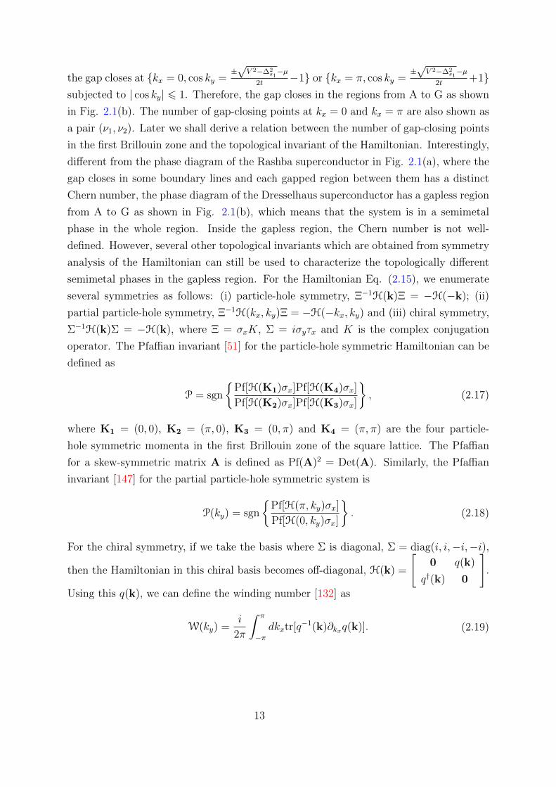
the gap closes at kx = 0, cos ky =±√V 2−∆2

s1−µ

2t−1 or kx = π, cos ky =

±√V 2−∆2

s1−µ

2t+1

subjected to | cos ky| 6 1. Therefore, the gap closes in the regions from A to G as shown

in Fig. 2.1(b). The number of gap-closing points at kx = 0 and kx = π are also shown as

a pair (ν1, ν2). Later we shall derive a relation between the number of gap-closing points

in the first Brillouin zone and the topological invariant of the Hamiltonian. Interestingly,

different from the phase diagram of the Rashba superconductor in Fig. 2.1(a), where the

gap closes in some boundary lines and each gapped region between them has a distinct

Chern number, the phase diagram of the Dresselhaus superconductor has a gapless region

from A to G as shown in Fig. 2.1(b), which means that the system is in a semimetal

phase in the whole region. Inside the gapless region, the Chern number is not well-

defined. However, several other topological invariants which are obtained from symmetry

analysis of the Hamiltonian can still be used to characterize the topologically different

semimetal phases in the gapless region. For the Hamiltonian Eq. (2.15), we enumerate

several symmetries as follows: (i) particle-hole symmetry, Ξ−1H(k)Ξ = −H(−k); (ii)

partial particle-hole symmetry, Ξ−1H(kx, ky)Ξ = −H(−kx, ky) and (iii) chiral symmetry,

Σ−1H(k)Σ = −H(k), where Ξ = σxK, Σ = iσyτx and K is the complex conjugation

operator. The Pfaffian invariant [51] for the particle-hole symmetric Hamiltonian can be

defined as

P = sgn

Pf[H(K1)σx]Pf[H(K4)σx]

Pf[H(K2)σx]Pf[H(K3)σx]

, (2.17)

where K1 = (0, 0), K2 = (π, 0), K3 = (0, π) and K4 = (π, π) are the four particle-

hole symmetric momenta in the first Brillouin zone of the square lattice. The Pfaffian

for a skew-symmetric matrix A is defined as Pf(A)2 = Det(A). Similarly, the Pfaffian

invariant [147] for the partial particle-hole symmetric system is

P(ky) = sgn

Pf[H(π, ky)σx]

Pf[H(0, ky)σx]

. (2.18)

For the chiral symmetry, if we take the basis where Σ is diagonal, Σ = diag(i, i,−i,−i),

then the Hamiltonian in this chiral basis becomes off-diagonal, H(k) =

[0 q(k)

q†(k) 0

].

Using this q(k), we can define the winding number [132] as

W(ky) =i

2π

ˆ π

−πdkxtr[q

−1(k)∂kxq(k)]. (2.19)

13

The Pfaffian invariant P can be used for identifying topologically different semimetal

phases of the Hamiltonian Eq. (2.15). It is easy to check that PA = PB = PC = PD = −1

and PE = PF = PG = 1 in the phase diagram of the Dresselhaus superconductor as shown

in Fig. 2.1(b). Therefore, the semimetal phases in the region of A, B, C, D and the region

of E, F, G are topologically inequivalent. As for the other two topological invariants P(ky)

and W(ky), below we shall show that they can be used to determine the range of edge

states in the edge Brillouin zone.

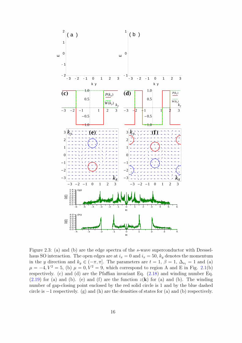
To demonstrate the novel properties in the semimetal phase of the Dresselhaus su-

perconductor, we study the Majorana Fermions at the edge and in the vortex core of it.

We first study the Majorana flat bands at the edge of the Dresselhaus superconductor.

By diagonalizing the Hamiltonian Eq. (2.12) with the parameters α = 0, ∆d1 = ∆d2 = 0

and Vz = 0, we get the edge spectra of the Dresselhaus superconductor. Interestingly, al-

though the gap closes in the semimetal phase from region A to G as shown in Fig. 2.1(b),

there exist Majorana flat bands at the edge of the system. The Majorana flat bands

in the two topologically different semimetal phases in the region A and E are depicted

in Fig. 2.3(a) and 2.3(b) respectively. Second, we would like to study the number and

range of the Majorana flat bands in these two different semimetal phases. By the Pfaffian

invariant Eq. (2.18) or winding number Eq. (2.19), the range where the Majorana flat

bands exist in the edge Brillouin zone can be exactly obtained as shown in Fig. 2.3(c) and

2.3(d). The number of Majorana flat bands is half of the number of gap-closing points

in the first Brillouin zone. From the Hamiltonian in the chiral basis, we can see that the

gap closes when Det q(k) = 0. In the complex plane of z(k) = Det q(k)/|Det q(k)|, a

winding number can be assigned to each gap-closing point k0 as

W(k0) =1

2πi

‰γ

dz(k)

z(k)− z(k0), (2.20)

where γ is a contour enclosing the gap-closing point. Due to the particle-hole symmetry,

W(k0) = −W(−k0); therefore, the gap-closing points with opposite winding number are

equal in number. The function z(k) in the region A and E are shown in Fig. 2.3(e)

and 2.3(f). As long as the projection of opposite winding number gap-closing points

does not completely overlap in the edge Brillouin zone, there will be Majorana flat bands

connecting them [161]. Therefore, the number of Majorana flat bands is ν = (ν1 + ν2)/2

and it is easy to check that the Pfaffian invariant P in Eq. (2.17) is the parity of ν,

P = (−1)ν . The corresponding densities of states of these two different semimetal phases

are shown in Fig. 2.3(g) and 2.3(h). We find that there is a peak at zero energy which

14

is clearly visible in the tunneling conductance measurements. Therefore, the Majorana

flat bands have clear experimental signature in the tunneling conductance measurements

and should be experimentally observable. As for the robustness of the Majorana flat

bands against disorder or impurity, we can discuss it from the topological point of view.

As long as the disorder or impurity does not break the symmetries of Hamiltonian Eq.

(2.15), these Majorana flat bands will be protected by the three topological invariants

mentioned above.

The existence of the edge states implies the nontrivial momentum space topology in

the Dresselhaus superconductor so that the Majorana fermions emerge at the edge of the

system. In the following, we explicitly calculate the zero-energy Majorana flat bands at

the edge of the Dresselhaus superconductor in the cylindrical symmetry. Let x-direction

to be open and y to be periodic, then by setting kx → −i∂x, we solve the Schrodinger

equation of the Hamiltonian Eq. (2.15) in the real space, H(kx → −i∂x, ky)Ψ = 0, where

Ψ = (u↑, u↓, v↑, v↓)T . Due to the particle-hole symmetry in the Dresselhaus superconduc-

tor, we have u↑ = v∗↑ and u↓ = v∗↓ at zero energy. Thus, we only need to consider the

upper block of the Hamiltonian Eq. (2.15). For simplicity, we consider the low energy

theory at kx = 0, up to the first order, we have

(ε(ky)− iβ∂x)u↑ + (Vx − iVy)u↓ + ∆s1u∗↓ = 0,

(ε(ky) + iβ∂x)u↓ + (Vx + iVy)u↑ −∆s1u∗↑ = 0,

(2.21)

where ε(ky) = −2t(1 + cos ky) − µ. Observing that u↑ = ±iu∗↓ in Eq. (2.21), we obtain

when u↑ = iu∗↓, the solution is u↑(x) = c1u1↑(x)+c2u

2↑(x), where c1 and c2 are real numbers

and

u1↑(x) = A1e

λ1x + A2eλ2x,

u2↑(x) = iB1e

λ1x + iB2eλ2x.

(2.22)

Here

λ1 =−∆s1 −

√V 2 − ε2(ky)

β,

λ2 =−∆s1 +

√V 2 − ε2(ky)

β,

(2.23)

15

- 3 - 2 - 1 0 1 2 3- 2

- 1

0

1

2

- 3 - 2 - 1 0 1 2 3- 1

0

1( a )

E

k y

( b )

E

k y

c Pky

W ky ky

-3 -2 -1 1 2 3

-1.0

-0.5

0.5

1.0 d Pky

Wkyky

-3 -2 -1 1 2 3

-1.0

-0.5

0.5

1.0

e

kx

ky

-3 -2 -1 0 1 2 3

-3

-2

-1

0

1

2

3 f

kx

ky

-3 -2 -1 0 1 2 3

-3

-2

-1

0

1

2

3

- 6 - 5 - 4 - 3 - 2 - 1 0 1 2 3 4 5 60 . 00 . 20 . 40 . 60 . 81 . 01 . 21 . 41 . 6

D(E)

( g )

E

- 4 - 3 - 2 - 1 0 1 2 3 40 . 00 . 51 . 01 . 52 . 02 . 53 . 03 . 54 . 0 ( h )

D(E)

E

Figure 2.3: (a) and (b) are the edge spectra of the s-wave superconductor with Dressel-haus SO interaction. The open edges are at ix = 0 and ix = 50, ky denotes the momentumin the y direction and ky ∈ (−π, π]. The parameters are t = 1, β = 1, ∆s1 = 1 and (a)µ = −4, V 2 = 5, (b) µ = 0, V 2 = 9, which correspond to region A and E in Fig. 2.1(b)respectively. (c) and (d) are the Pfaffian invariant Eq. (2.18) and winding number Eq.(2.19) for (a) and (b). (e) and (f) are the function z(k) for (a) and (b). The windingnumber of gap-closing point enclosed by the red solid circle is 1 and by the blue dashedcircle is −1 respectively. (g) and (h) are the densities of states for (a) and (b) respectively.

16

and

A1 =1

2

[1− Vx − i(Vy + ε)√

V 2 − ε2

], A2 =

1

2

[1 +

Vx − i(Vy + ε)√V 2 − ε2

],

B1 =1

2

[1 +

Vx − i(Vy − ε)√V 2 − ε2

], B2 =

1

2

[1− Vx − i(Vy − ε)√

V 2 − ε2

].

(2.24)

When u↑ = −iu∗↓, the solution is similar to the case of u↑ = iu∗↓. We consider the

Dresselhaus superconductor in the positive x plane with the edge located at x = 0. Let

us assume ∆s1 > 0 for simplicity, then from the solutions to Eq. (2.21), the critical point

for existing a normalizable wavefunction under this boundary condition is determined by

V 2−ε(ky)2 = ∆2s1

, which is consistent with the gap-closing condition (µ+2t+2t cos ky)2+

∆2s1

= V 2 at kx = 0. By the same reason, the condition for normalizable wavefunctions is

consistent with the gap-closing condition (µ−2t+2t cos ky)2+∆2

s1= V 2 if we consider the

low energy theory at kx = π. Therefore, the Majorana flat band is (u↑, iu∗↑, u∗↑,−iu↑)T ,

where u↑ is the solution to Eq. (2.21).

To further study the Majorana fermions in the Dresselhaus superconductor, we con-

sider the zero energy vortex core states by solving the BdG equation for the supercon-

ducting order parameter of a single vortex ∆(r, θ) = ∆eiθ [128]. To do this, the s-wave

superconducting term in the Hamiltonian Eq. (2.2) is modified to be position-dependent,

Hs =∑i

(∆eiθic†i↑c†i↓ + H.c.). (2.25)

We numerically solve the Schrodinger equation HΨ = EΨ for the Hamiltonian in Eq.

(2.15) in real space, where Ψ = (u↑, u↓, v↑, v↓)T . At zero energy we have u↑ = v∗↑ and u↓ =

v∗↓ as the particle-hole symmetry in the Dresselhaus superconductor, then the Bogoliubov

quasiparticle operator,

γ†(E) =∑i

(ui↑c†i↑ + ui↓c

†i↓ + vi↑ci↑ + vi↓ci↓) (2.26)

becomes Majorana operator γ†(0) = γ(0). Below we only consider the zero energy vortex

core states for discussing the MFs in the vortex core. Setting the x and y directions to be

open boundary, we then solve the BdG equations numerically and calculate the density

profile of quasiparticle for the zero energy vortex core states. The density of quasiparticle

at site i is defined as u∗i↑ui↑ + u∗i↓ui↓. Previously, we have shown in Fig. 2.3 that there

is a novel semimetal phase in the Dresselhaus superconductor where the zero-energy flat

17

5 1 0 1 5 2 0 2 5 3 0 3 5 4 0

51 01 52 02 53 03 54 0 ( a )

0

0 . 0 1 1

5 1 0 1 5 2 0 2 5 3 0 3 5 4 0

51 01 52 02 53 03 54 0

0

0 . 0 0 2 6( b )

Figure 2.4: The probability distribution of quasiparticle for the Dresselhaus supercon-ductor plotted on the 41× 41 square lattice. The parameters are t = 1, β = 1, ∆s1 = 1.The chemical potential and in-plane magnetic field are (a) µ = −4, V 2 = 5 and (b)µ = 0, V 2 = 9.

bands host MFs. Here we shall ascertain if there exist zero energy vortex core states

hosting MFs in this semimetal phase. The density profiles of quasiparticle of the zero

energy vortex core states are shown in Fig. 2.4(a) and 2.4(b), which correspond to the

region A and E in the phase diagram of Fig. 2.1(b) respectively. The numerical results

of the energy for the zero energy vortex core states are E = 2.54 × 10−3 for Fig. 2.4(a)

and E = 6.68 × 10−3 for Fig. 2.4(b) respectively. It is clear to see from Fig. 2.4 that

there are zero-energy states in the vortex core. Therefore, the Majorana fermions exist

in the vortex core of the s-wave Dresselhaus superconductor.

2.5 Topological properties of the spin-singlet super-

conductor

2.5.1 symmetries of the BdG Hamiltonian

For the general BdG Hamiltonian of the spin-singlet superconductor Eq. (2.7), it

satisfies the particle-hole symmetry

Ξ−1H(k)Ξ = −H(−k), (2.27)

where Ξ = ΛK, Λ = σx ⊗ τ0 and K is the complex conjugation operator. We find

that apart from the particle-hole symmetry, the BdG Hamiltonian can satisfy some extra

18

symmetries, namely, partial particle-hole symmetry, chiral symmetry and partial chiral

symmetry when some parameters in the Hamiltonian Eq. (2.7) are vanishing. The

particle-hole-kx and particle-hole-ky symmetries are defined as

Ξ−1kxH(kx, ky)Ξkx = −H(−kx, ky) (2.28)

and

Ξ−1kyH(kx, ky)Ξky = −H(kx,−ky), (2.29)

where Ξkx (Ξky) takes the kx (ky) in the Hamiltonian to −kx (−ky). The chiral symmetry

is given by

Σ−1H(k)Σ = −H(k). (2.30)

The chiral-kx and chiral-ky symmetries are defined as

Σ−1kxH(kx, ky)Σkx = −H(−kx, ky) (2.31)

and

Σ−1kyH(kx, ky)Σky = −H(kx,−ky), (2.32)

where Σkx (Σky) takes the kx (ky) in the Hamiltonian to −kx (−ky).We are interested in the BdG Hamiltonian which has one or more extra symmetries.

In the following, we would like to consider these kinds of the BdG Hamiltonian as listed

in Tab. 2.1. The spin-singlet superconductor with Rashba spin-orbit coupling has been

investigated in Ref. [131]. Here we only consider the general dx2−y2 + idxy + s pairing in

case (a) for the spin-singlet Rashba superconductor. We shall focus on the topological

properties of the superconductor with Dresselhaus (110) spin-orbit coupling as shown in

case (b)-(g) of Tab. 2.1.

2.5.2 topological invariants of the BdG Hamiltonian

For the fully gapped Hamiltonian, we can always define the Chern number as a topo-

logical invariant of the Hamiltonian as shown in Eq. (2.9). If the Hamiltonian has some

19

case spin-orbit coupling magnetic field pairing symmetry Hamiltonian symmetry topological invariant(a) α Vz ∆s1 ,∆d1 ,∆d2 Ξ,Σkx P, W(b)

β Vx, Vy

∆s1 Ξ,Ξkx ,Σ,Σky P, P(ky), W, W(ky)(c) ∆s1 ,∆s2 Ξ,Ξkx P, P(ky)(d) ∆d1 Ξ,Ξkx ,Σ,Σky P, P(ky), W, W(ky)(e) ∆d1 ,∆d2 Ξ,Σky P, W(f) ∆s1 ,∆d1 Ξ,Ξkx ,Σ P, P(ky), W(ky)(g) ∆s1 ,∆d1 ,∆d2 Ξ,Σky P, W

Table 2.1: The BdG Hamiltonian with extra symmetries, namely, the particle-hole sym-metry and the particle-hole-kx symmetry, Ξ = Ξkx = σxK, the chiral symmetry and thechiral-ky symmetry, Σ = Σky = iσyτx, and the chiral-kx symmetry, Σkx = iσyτz. Thetopological invariants corresponding to these extra symmetries are also shown in the lastcolumn.

extra symmetries, more topological invariants can be introduced into the system.

We first consider the particle-hole symmetry Eq. (2.27) which can be reduced to

ΛH(k)Λ = −H∗(−k). We find that under this symmetry H(K)Λ is an antisymmetric

matrix with (H(K)Λ)T = −H(K)Λ, where K is the particle-hole symmetric momenta

satisfying K = −K + G and G is the reciprocal lattice vector of the square lattice.

With this property, we can define the Pfaffian invariant for the particle-hole symmetric

Hamiltonian as [51]

P = sgn

Pf[H(K1)Λ]Pf[H(K4)Λ]

Pf[H(K2)Λ]Pf[H(K3)Λ]

, (2.33)

where K1 = (0, 0), K2 = (π, 0), K3 = (0, π) and K4 = (π, π) are the four particle-hole

symmetric momenta in the first Brillouin zone of the square lattice. Here we shall show

that the Pfaffian invariant P is the parity of the Chern number C, P = (−1)C. For the

2n× 2n antisymmetric matrix H(K)Λ, we have Pf[H(K)Λ]∗ = (−1)nPf[H(K)Λ]. There-

fore, (inPf[H(K)Λ])∗ = inPf[H(K)Λ] is real and we can associate a quantity S[H(K)] =

sgninPf[H(K)Λ] with any particle-hole symmetric Hamiltonian. Suppose H(K) is di-

agonalized by the transformation H(K) = U(K)D(K)U †(K), where D(K) is a diagonal

matrix of eigenvalues diagEn(K), · · ·, E1(K),−E1(K), · · ·,−En(K) and the columns of

the unitary matrix U(K) are the eigenvectors of H(K). The eigenvectors for the positive

eigenvalues in U(K) are chosen to be related to the eigenvectors for negative eigenvalues

by the particle-hole symmetry [131]. With this convention, we find that U †Λ = ΓUT ,

20

where Γ = σxτx. Therefore, S[H(K)] can be further reduced to

S[H(K)] = sgninPf[H(K)Λ],

= sgninPf[U(K)D(K)U †(K)Λ],

= sgninPf[U(K)D(K)ΓUT (K)],

= sgnin DetU(K)Pf[D(K)Γ].

(2.34)

Since Pf[D(K)Γ] =∏

n>0En(K) > 0 and |DetU(K)| = 1, we arrive at

S[H(K)] = in DetU(K). (2.35)

Note that A(k) = i∑

n〈ψn(k)|∇ψn(k)〉 is a total derivative [131], A(k) = i∇ ln[DetU(k)].

Therefore, consider a pair of particle-hole symmetric momenta K1 and K2, we find that

DetU(K2)

DetU(K1)= e−iS1,2 , (2.36)

where S1,2 =´ K2

K1A(k) · dk and the line integral runs from K1 to K2. Since A+(k) =

i∑

n>0〈ψn(k)|∇ψn(k)〉 = A−(−k), we find that S1,2 =´γ1

A−(k) · dk, where γ1 is the

line from (−π, 0) to (π, 0). Similarly,

DetU(K4)

DetU(K3)= e−iS3,4 , (2.37)

where S3,4 =´γ2

A−(k) · dk and γ2 is the line from (−π, π) to (π, π). Therefore,

DetU(K1) DetU(K4)

DetU(K2) DetU(K3)= eiSγ , (2.38)

where Sγ =γA−(k) · dk and γ is the directed line surrounding the upper half Brillouin

zone (UHBZ) in the anticlockwise direction. Since F−(k) = ∂kxA−y (k) − ∂kyA

−x (k) =

21

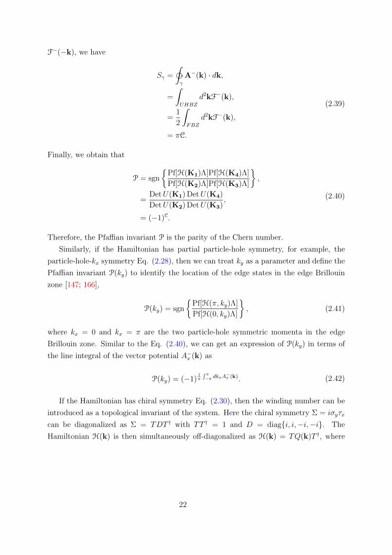
F−(−k), we have

Sγ =

‰γ

A−(k) · dk,

=

ˆUHBZ

d2kF−(k),

=1

2

ˆFBZ

d2kF−(k),

= πC.

(2.39)

Finally, we obtain that

P = sgn

Pf[H(K1)Λ]Pf[H(K4)Λ]

Pf[H(K2)Λ]Pf[H(K3)Λ]

,

=DetU(K1) DetU(K4)

DetU(K2) DetU(K3),

= (−1)C.

(2.40)

Therefore, the Pfaffian invariant P is the parity of the Chern number.

Similarly, if the Hamiltonian has partial particle-hole symmetry, for example, the

particle-hole-kx symmetry Eq. (2.28), then we can treat ky as a parameter and define the

Pfaffian invariant P(ky) to identify the location of the edge states in the edge Brillouin

zone [147; 166],

P(ky) = sgn

Pf[H(π, ky)Λ]

Pf[H(0, ky)Λ]

, (2.41)

where kx = 0 and kx = π are the two particle-hole symmetric momenta in the edge

Brillouin zone. Similar to the Eq. (2.40), we can get an expression of P(ky) in terms of

the line integral of the vector potential A−x (k) as

P(ky) = (−1)1π

´ π−π dkxA

−x (k). (2.42)

If the Hamiltonian has chiral symmetry Eq. (2.30), then the winding number can be

introduced as a topological invariant of the system. Here the chiral symmetry Σ = iσyτx

can be diagonalized as Σ = TDT † with TT † = 1 and D = diagi, i,−i,−i. The

Hamiltonian H(k) is then simultaneously off-diagonalized as H(k) = TQ(k)T †, where

22

Q(k) is of the form

[0 q(k)

q†(k) 0

]. We can thus define the winding number as

W(ky) = − 1

4π

ˆ π

−πdkxtr[ΣH−1(k)∂kxH(k)],

= − 1

4π

ˆ π

−πdkxtr[DQ

−1(k)∂kxQ(k)],

=i

4π

ˆ π

−πdkxtr[q

−1(k)∂kxq(k)− q†−1(k)∂kxq†(k)],

= − 1

2πIm

ˆ π

−πdkxtr[q

−1(k)∂kxq(k)].

(2.43)

Here we show that´ π−π dkxtr[q

−1(k)∂kxq(k)] is pure imaginary. It is easy to see that

tr[q−1∂kxq]∗ = −tr[q†∂kxq

†−1]. From the eigen equation of Q(k), we find that qq†|ψn〉 =

E2n|ψn〉 which leads to the identity qq†Ψ = ΨΠ, where Π = diagE2

1 , E22 and the unitary

matrix Ψ = (|ψ1〉, |ψ2〉). Therefore, q† = q−1ΨΠΨ−1 and we obtain tr[q†∂kxq†−1] =

tr[q−1∂kxq] + tr[Π∂kxΠ−1]; accordingly,

ˆ π

−πdkxtr[q

−1∂kxq]∗ =−

ˆ π

−πdkxtr[q

−1∂kxq]−ˆ π

−πdkxtr[Π∂kxΠ

−1]. (2.44)

Due to the periodic boundary condition, we have En(kx = −π, ky) = En(kx = π, ky) so

that

ˆ π

−πdkxtr[Π∂kxΠ

−1] = −22∑

n=1

ˆ π

−πdkx∂kx lnEn(k) = 0. (2.45)

Thus´ π−π dkxtr[q

−1∂kxq]∗ = −

´ π−π dkxtr[q

−1∂kxq] is pure imaginary. Finally, the winding

number for the chiral symmetry Eq. (2.30) is obtained,

W(ky) = − 1

2πi

ˆ π

−πdkxtr[q

−1(k)∂kxq(k)]. (2.46)

When the Hamiltonian has partial particle-hole symmetry and chiral symmetry simulta-

neously, we can find a relation between the Pfaffian invariant P(ky) and the winding num-

ber W(ky). According to the Ref. [131], 1π

´ π−π A

−x (k) = 1

2πi

´ π−π tr[q(k)−1∂kxq(k)] + 2N ,

where N is an integer. Substituting this relation into Eq. (2.42), we get that P(ky) =

(−1)W(ky). Therefore, the Pfaffian invariant P(ky) is the parity of the winding number

W(ky).

23

If the Hamiltonian has partial chiral symmetry, for example, the chiral-ky symmetry

Eq. (2.32), then we can only define the winding number W(ky) at ky = 0 and ky = π.

Consequently, we can associate a topological invariant W with the chiral-ky symmetry as

[131]

W = (−1)W(0)−W(π). (2.47)

The topological invariant W is also the parity of the Chern number, W = (−1)C. There-

fore, the Pfaffian invariant P for the particle-hole symmetry is equivalent to the topolog-

ical invariant W for the partial chiral symmetry.

2.5.3 phase diagrams of the BdG Hamiltonian

In contrast to the even number of Majorana bound states in the trivial topological

phase, the number of Majorana bound states is odd in the nontrivial topological phase.

The Pfaffian invariant P is in fact the parity of the number of Majorana bound states.

Therefore, we can use the Pfaffian invariant P to investigate the topological quantum

phase transitions in the BdG Hamiltonian Eq. (2.7). The phase diagrams are shown in

Fig. 2.5. We now focus on the red region where the Pfaffian invariant P = −1 which

means that the system has an odd number of Majorana bound states at the edge and is

thus in the nontrivial topological phase. The explicit expression of the Pfaffian invariant

Eq. (2.33) for the general case of the BdG Hamiltonian is

P = sgn

[(µ+ 4t)2 + (∆2

s1+ ∆2

s2)− V 2][(µ− 4t)2 + (∆2

s1+ ∆2

s2)− V 2]

[µ2 + (∆s1 + 2∆d1)2 + ∆2s2− V 2][µ2 + (∆s1 − 2∆d1)2 + ∆2

s2− V 2]

. (2.48)

Therefore, the phase diagram is divided by the following four parabolas in the plane of

V 2 ∼ µ:

(i)V 2 = (µ+ 4t)2 + (∆2s1

+ ∆2s2

);

(ii)V 2 = (µ− 4t)2 + (∆2s1

+ ∆2s2

);

(iii)V 2 = µ2 + (∆s1 + 2∆d1)2 + ∆2s2

;

(iv)V 2 = µ2 + (∆s1 − 2∆d1)2 + ∆2s2,

(2.49)

where V 2 = V 2x + V 2

y + V 2z . Notice that the Pfaffian invariant P has nothing to do with

the spin-orbit couplings. Thus the topological phases can exist even without the spin-

orbit couplings. However, the spin-orbit couplings can open a gap to render the Majorana

24

a Μ

V 2

O

I II

-10 -5 0 5 100

10

20

30

40

50

b Μ

V 2

O

I

II

III

-10 -5 0 5 100

20

40

60

80

c Μ

V 2

O

I

II

III

IV

-6 -4 -2 0 2 4 60

10

20

30

40

d Μ

V 2

O

I

II

III

-10 -5 0 5 100

20

40

60

80

100

Figure 2.5: The possible phase diagrams of the spin-singlet superconductor with Rashbaand Dresselhaus (110) spin-orbit couplings. (a) is the phase diagram for the pure s-waveor d-wave superconductor. (b), (c) and (d) are the phase diagrams for the d + s-wavesuperconductor.

fermion located at the edge of the system; otherwise the Majorana fermion will spread into

the bulk. Now we turn to discuss all the possible phase diagrams in the BdG Hamiltonian.

When ∆s1∆d1 = 0, the phase diagram is only divided by the parabolas (i) and (ii) and is

shown in Fig. 2.5(a). When ∆s1∆d1 6= 0, there are three topologically different cases in

the phase diagrams as follows. Let us first define the intersection point of the parabolas

(i) and (ii) as O, then the phase diagram where the parabolas (iii) and (iv) are both below

O is shown in Fig. 2.5(b); the phase diagram where the parabolas (iii) and (iv) are on

either side of O is shown in Fig. 2.5(c); the phase diagram where the parabolas (iii) and

(iv) are both above O is shown in Fig. 2.5(d). Furthermore, if we assume ∆s1∆d1 > 0,

then the phase diagram is as Fig. 2.5(b) when ∆2d1− ∆s1∆d1 < ∆2

d1+ ∆s1∆d1 < 4t2;

the phase diagram is as Fig. 2.5(c) when ∆2d1− ∆s1∆d1 < 4t2 < ∆2

d1+ ∆s1∆d1 ; the

phase diagram is as Fig. 2.5(d) when 4t2 < ∆2d1− ∆s1∆d1 < ∆2

d1+ ∆s1∆d1 . Therefore,

we have exhibited all the possible phase diagrams in the BdG Hamiltonian Eq. (2.7).

For the pure s-wave and d-wave superconductors, the phase diagrams are topologically

equivalent to Fig. 2.5(a); for the superconductors with mixed s-wave and d-wave pairing

symmetries, the phase diagrams are topologically equivalent to Fig. 2.5(b), Fig. 2.5(c)

and Fig. 2.5(d) depending on the hopping amplitude t.

2.5.4 Majorana bound states at the edge of the BdG Hamilto-

nian

In this section, we demonstrate the Majorana bound states at the edge of the spin-

singlet superconductor in the different cases as listed in Tab. 2.1. By setting the boundary

conditions of x direction to be open and y direction to be periodic, we diagonalize the

25

Hamiltonian Eq. (2.7) in this cylindrical symmetry and get the edge spectra of the

Hamiltonian. Generally, the solution is Ψ = (Ψ1, · · ·,ΨNx)T , where Nx is the number

of unit cells in the x direction and Ψi = (ui↑, ui↓, vi↑, vi↓) is the wave function at cell

i. In particular, at zero energy we have u↑ = v∗↑ and u↓ = v∗↓ due to the particle-hole

symmetry in the superconductor, then the Bogoliubov quasiparticle operator, γ†(E) =∑j=(ix,ky)(uj↑c

†j↑ + uj↓c

†j↓ + vj↑cj↑ + vj↓cj↓), becomes Majorana operator γ†(0) = γ(0).

Therefore, once the zero-energy states exists in the edge spectrum, the Majorana fermion

will emerge at the edge of the system.

We first discuss the pure s-wave and d-wave superconductors in case (b)-(e) of Tab.

2.1. Note that the appearance of imaginary part of the superconducting gap function,

∆s2 and ∆d2 , will lower the symmetry of the BdG Hamiltonian Eq. (2.7) by breaking

the chiral symmetry or partial particle-hole symmetry. The four topological indices, P,

W, P(ky) and W(ky), play different roles in characterizing the topological properties

of the system. On one hand, P or W can be interpreted as a bulk index to indicate

whether or not a region in the phase diagram is topological; on the other hand, P(ky) or

W(ky) serves as an edge index to indicate that if there exists topological phase at each

ky in the edge Brillouin zone. More specifically, when P(ky) = −1 or W(ky) is odd, the

Hamiltonian is topologically nontrivial and the Majorana bound states will emerge at

some range of ky. Therefore, these continuous zero-energy Majorana bound states in the

edge Brillouin zone will form a stable Majorana flat band when the edge index exists.

Note that the winding number W(ky) can be changed by some even number in the same

phase. However, its parity, the Pfaffian invariant P(ky) is unchanged in the same phase

since P(ky) = (−1)W(ky). The phase diagrams of case (b)-(e) are topologically equivalent

and shown in Fig. 2.5(a). From Tab. 2.1, we find that there exists edge index, P(ky) or

W(ky), in all cases except case (e). Therefore, the edge spectra of pure s-wave and dx2−y2-

wave superconductors are Majorana flat bands and exhibited in Fig. 2.6(a) and 2.6(c)

which correspond to case (c) and (d) respectively. From the edge spectra, we observe

that there are odd number of Majorana flat bands in the nontrivial topological phase.

The edge indices, P(ky) and/or W(ky), are also depicted in Fig. 2.6(b) and 2.6(d). We

find that there is only one edge index survived in case (c) due to the breaking of chiral

symmetry. Comparing the edge spectra with the edge indices in Fig. 2.6(a)-2.6(d), we can

see that the location of the Majorana flat bands is consistent with the Pfaffian invariant

P(ky) and/or the winding number W(ky). In addition, due to the lack of edge index in

the dx2−y2 + idxy-wave superconductor, the Majorana flat band disappears and becomes

Dirac cone as shown in Fig. (2.7).

26

Figure 2.6: The edge spectra and topological invariants of the spin-singlet superconductorwith Dresselhaus (110) spin-orbit coupling. The open edges are at ix = 0 and ix = 50,ky denotes the momentum in the y direction and ky ∈ (−π, π]. (a) is the edge spectrumof s-wave superconductor. The parameters are t = 1, β = 1, ∆s1 = 1, ∆s2 = 1, µ = 0,V 2 = 9 and correspond to a point in region II of Fig. 2.5(a). (c) is the edge spectrumof dx2−y2-wave superconductor. The parameters are t = 1, β = 1, ∆d1 = 1, ∆d2 = 0,µ = −4, V 2 = 9 and correspond to a point in region I of Fig. 2.5(a). (e) and (g) arethe edge spectra of dx2−y2 + s-wave superconductor. The parameters are β = 1, ∆s1 = 1,∆d1 = 2 and (e) t = 2, µ = 0, V 2 = 16, (g) t = 1, µ = −4.5, V 2 = 25 which correspond toregion I of Fig. 2.5(b) and region IV of Fig. 2.5(c) respectively. (b), (d), (f) and (h) arethe Pfaffian invariant P(ky) and/or winding number W(ky) for the corresponding cases.

- 3 - 2 - 1 0 1 2 3- 1 . 0

- 0 . 5

0 . 0

0 . 5

1 . 0 ( a )

E

k y- 3 - 2 - 1 0 1 2 3- 0 . 5 0

- 0 . 2 5

0 . 0 0

0 . 2 5

0 . 5 0 ( b )

E

k y

Figure 2.7: (a) and (b) are the edge spectra of the dx2−y2 + idxy-wave superconductorwith Dresselhaus (110) spin-orbit coupling in case (e). The parameters are t = 1, β = 1,∆d1 = 1, ∆d2 = 1 and (a) µ = −4, V 2 = 9, (b) µ = 0, V 2 = 9, which correspond toregions I and II in Fig. 2.5(a).

27

We now turn to discuss the superconductors with mixed s-wave and d-wave pairing

symmetries as listed in case (a), (f) and (g) of Tab. 2.1. For each case, there are three

different kinds of phase diagrams depending on the hopping amplitude t as demonstrated

in Fig. 2.5(b)-2.5(d). The edge spectra for the mixed pairing superconductors are similar

to their pure pairing counterparts. Notice that the Majorana flat bands will emerge

only in dx2−y2 + s-wave superconductor in case (f) because in the other two cases there

is no edge index to make the Majorana flat bands stable. The edge spectra for the

dx2−y2 + s-wave superconductor with Dresselhaus (110) spin-orbit coupling are shown

in Fig. 2.6(e) and 2.6(g) which correspond to region I in Fig. 2.5(b) and region IV in

Fig. 2.5(c) respectively. The edge indices associated with them are also depicted in Fig.

2.6(f) and 2.6(h) (for fully details of this case, please see Appendix A). Note that the

winding number W(ky) in some range of ky can be 2, however, it is topologically trivial

because its parity, namely the Pfaffian invariant P(ky) is 1. For the dx2−y2 + idxy +s-wave

superconductor with Rashba/Dresselhaus (110) spin-orbit coupling in case (a) and (g),

without the protection of edge indices, the edge spectra become Dirac cones and have no

qualitative differences to the dx2−y2 + idxy-wave superconductor. We have put the details

into Appendix A.

Comparing the edge spectra with the edge indices in Fig. 2.6, we find that the location

of Majorana flat bands can be determined by the edge indices. This result holds true for

the switched boundary condition, namely, periodic boundary in the x direction and open

in the y direction. From the symmetries of Hamiltonian exhibited in Tab. 2.1, only for

the Hamiltonian with chiral symmetry Eq. (2.30) can we define edge index W(kx) in the

switched boundary condition,

W(kx) = − 1

4π

ˆ π

−πdkytr[ΣH−1(k)∂kyH(k)],

= − 1

2πi

ˆ π

−πdkytr[q

−1(k)∂kyq(k)].

(2.50)

Therefore, we will consider cases (b), (d) and (f) in the switched boundary condition.

It is worth noting that W(kx) is always zero in these three cases. Thus we obtain an

interesting result that the Majorana flat bands only exist along the y direction. This is

due to the space asymmetry of Dresselhaus (110) spin-orbit coupling Eq. (2.5). Here

we directly give the edge spectra and edge index in the switched boundary condition as

shown in Fig. 2.8. The parameters chosen in Fig. 2.8 are the same as the one in Fig.

2.6 except that Fig. 2.8(a) is the same as Fig. 2.3(a). We can see that W(kx) = 0 in

28

Figure 2.8: The edge spectra and edge index in the switched boundary condition. Theopen edges are at iy = 0 and iy = 100, kx denotes the momentum in the x direction andkx ∈ (−π, π]. (a) is the edge spectrum of the s-wave superconductor. The parameters aret = 1, β = 1, ∆s1 = 1, ∆s2 = 0, µ = −4, V 2 = 5 and correspond to a point in region I ofFig. 2.5(a). (b) is the edge spectrum of the dx2−y2-wave superconductor. The parametersare t = 1, β = 1, ∆d1 = 1, ∆d2 = 0, µ = −4, V 2 = 9 and correspond to a point in regionI of Fig. 2.5(a). (c) is the edge spectrum of the dx2−y2 + s-wave superconductor. Theparameters are t = 1, β = 1, ∆s1 = 1, ∆d1 = 2, µ = −4.5, V 2 = 25 and correspond to apoint in region IV of Fig. 2.5(c). (d) is the edge index W(kx) = 0 for all the cases.

the whole edge Brillouin zone and there is no Majorana flat band along the x direction.

However, the parameters chosen are in the topological nontrivial phase and we indeed

find the Majorana flat bands along the y direction as shown in Fig. 2.6.

Notice that the Majorana flat band does not always situate at the edge of the system.

At a fixed ky, the bigger the gap of bulk state is, the more localized the Majorana

bound state is. Let us take the edge spectra of the dx2−y2-wave superconductor with

the Dresselhaus (110) spin-orbit coupling in Fig. 2.6(c) as an example. The probability

distribution of the quasiparticle at ky = 0, 1, 1.3 are shown in Fig. 2.9. From Fig. 2.6(c),

we see that the gap of the bulk state decreases as ky increases from 0 to 1.3. At the same

time, the probability distribution of the quasiparticle becomes more and more delocalized

and finally extends into the bulk. Therefore, only the big-gap Majorana bound states in

the flat bands are well-defined Majorana particles.

29

2468

1 0 ( a )

0

0 . 1

2468

1 0 ( b )| y i | 2

0

0 . 0 8

5 1 0 1 5 2 0 2 5 3 0 3 5 4 0 4 5 5 02468

1 0 ( c )

i x

0

0 . 0 2

Figure 2.9: The probability distributions of the Majorana fermion in the dx2−y2-wavesuperconductor with Dresselhaus (110) spin-orbit coupling in the edge Brillouin zone ofky = 0, 1, 1.3. ix is the lattice site. |ψix|2 is the probability of quasiparticle at site ix.

30

Chapter 3

Majorana transport in

superconducting nanowire with

Rashba and Dresselhaus spin-orbit

couplings

3.1 Introduction

An intensive search is ongoing in experimental realization of topological superconduc-

tor for topological quantum computing [3; 51; 90; 125; 130; 131; 134; 166; 169; 170]. The

basic idea is to embed qubit in a nonlocal, intrinsically decoherence-free way. The proto-

type is a spinless p-wave superconductor [70; 79; 80]. Edge excitations in such a state are

Majorana fermions (MFs) which obey non-Abelian statistics and can be manipulated by

braiding operations. The nonlocal MFs are robust against local perturbations and have

been proposed for topological quantum information processing [4; 24].

A hybrid semiconducting-superconducting nanostructure has become a mainstream

experimental setup recently for realizing topological superconductor and Majorana fermion

[3; 45; 99; 119; 134]. The signature of MFs characterized by a zero-bias conductance

peak (ZBP) has been reported in the tunneling experiments of the InSb nanowire [23;

27; 31; 40; 91; 109]. Motivated by this, we propose a two-lead setup for studying the

tunneling transport of MFs as shown in Fig. 3.1. A spin-orbit coupled InSb nanowire

is deposited on an s-wave superconductor. Due to the superconducting proximity ef-

fect, the wire is effectively equivalent to the spinless p-wave superconductor and hosts

31

Figure 3.1: Experimental setup for tunneling experiment. An InSb nanowire is depositedon an s-wave superconductor and coupled to two normal metal leads.

MFs at the ends. The nanowire is then coupled to two normal metal leads so as to

measure the currents. For our study, we apply the Keldysh non-equilibrium Green

function (NEGF) method to obtain the current response of the tunneling Hamiltonian

[12; 30; 32; 36; 42; 71; 86; 100; 106; 173; 175]. Curiously in the two-lead case, we ob-

serve that the currents at left and right leads are asymmetric as shown in Fig. 3.2.

This is due to the exotic commutation relation of MFs, γi, γj = 2δi,j. From another

standpoint, the zero-energy fermion b0 combined by the end-Majorana modes (γL,R) is

so highly nonlocal, b0 = (γL + iγR)/2, as to make the Majorana transport deviate from

the ordinary transport mediated by electron. Different from the ordinary one, there is

a hole transmission channel in Eq. (3.28) in Majorana transport. This makes the left

and right currents asymmetric. The current asymmetry may be used as a criterion to

further confirm the existence of Majorana fermion in our two-lead setup. We also give

the ac current response in the thesis and find that the current is enhanced in step with

the increase of level broadening and the decrease of temperature, and finally saturates

at high voltage. We use the bosonization and renormalization group (RG) methods to

consider the transport property of the Majorana nanowire with short-range Coulomb in-

teraction and disorder [20; 39; 44; 48; 52; 53; 69; 96; 97; 133; 145]. We observe that there

is a topological quantum phase transition under the interplay of superconductivity and

disorder. It is found that the Majorana transport is preserved in the superconducting-

dominated topological phase and destroyed in the disorder-dominated non-topological

insulator phase. The phase diagram and the condition in which the Majorana transport

exists are given.

The main results of this chapter were published in the following paper:

• Jia-Bin You, Xiao-Qiang Shao, Qing-Jun Tong, A. H. Chan, C. H. Oh, and Vlatko

32

Vedral, Majorana transport in superconducting nanowire with Rashba and Dres-

selhaus spin-orbit couplings. Journal of Physics: Condensed Matter 27, 225302

(2015).

3.2 Model

The model is depicted in Fig. 3.1. Two normal metal leads are connected to the

superconducting wire through ohmic contacts at the two ends. When the chemical po-

tential of superconducting wire lies within the energy gap, two MFs will appear at the

two ends of the wire respectively. The topological superconducting wire is made of a

spin-orbit coupled semiconductor (InSb wire) deposited on an s-wave superconducting

substrate. Via the superconducting proximity effect [45], the Cooper pair will tunnel

into the semiconductor and generate the s-wave superconductivity in the semiconducting

wire.

The one dimensional spin-orbit coupled s-wave superconducting nanowire can be mod-

eled as Hnw = H0 +H∆ [37; 145], where

H0 =

ˆdkΨ†k[ξk + (ατy + βτx)k + Vzτz]Ψk,

H∆ = ∆

ˆdk(ak↑a−k↓ + H.c.).

(3.1)

Here ξk = k2/2m− µ where k is the momentum and µ is the chemical potential, τx and

τy are spin Pauli matrices, α and β are the Rashba and Dresselhaus spin-orbit strengths,

∆ is the s-wave gap function and Ψk = (ak↑, ak↓)T where ak↑ (ak↓) is the annihilation

operator for spin up (down) electron. We also exert a perpendicular magnetic field Vz on

the wire and consider the Zeeman effect.

In the Nambu basis Φ†k = (Ψ†k,Ψ−k), the Hamiltonian Eq. (3.1) can be recast into

H = 12

´dkΦ†kH(k)Φk, where

H(k) = ξkτz + αkτzσy + βkσx + ∆τyσy + Vzτzσz. (3.2)

Here σx, σy and σz are the Pauli matrices in the particle-hole space. It is known that the

BdG Hamiltonian Eq. (3.2) satisfies the particle-hole symmetry, Ξ−1H(k)Ξ = −H(−k),

where Ξ = τxK and K is the complex conjugation operator [169; 170]. The topological

33

property of this BdG Hamiltonian can be examined by the Pfaffian invariant [79],

P = sgn Pf[H(k = 0)τx] = sgn(µ2 + ∆2 − V 2z ). (3.3)

Therefore, a topological quantum phase transition occurs when µ2 + ∆2 = V 2z . For

µ2 + ∆2 < V 2z , P = −1, the gap is dominated by the magnetic field and the wire is in the

topological phase with Majorana fermion at the ends of the nanowire. For µ2 + ∆2 > V 2z ,

P = 1, the gap is dominated by pairing with no end states. In this thesis, we study the

case where the nanowire is in the topological phase. This can be realized by putting the

chemical potential inside the energy gap. The low energy theory of the Hamiltonian Eq.

(3.1) can then be obtained as follow. By diagonalizing the Hamiltonian H0, we get two

energy bands, ε±(k) = k2

2m−µ±

√(α2 + β2)k2 + V 2

z . For these two bands, the eigenstates

are

|χ+(k)〉 =

[e−iθ/2 cos γk

2

eiθ/2 sin γk2

], |χ−(k)〉 =

[−e−iθ/2 sin γk

2

eiθ/2 cos γk2

], (3.4)

respectively, where tan θ = α/β and tan γk =√α2 + β2k/Vz. When the magnetic field

is dominant than the spin-orbit interactions (Vz α, β), γk ≈ 0, then the spins will be

forced to be nearly polarized within each band. Because the chemical potential lies within

the gap, only the low energy band is near the Fermi points and activated. We can thus

restrict the Hilbert space to the lower band in this case [45]. To achieve this, we unitarily

transform the electron operator from spin basis to band basis, (a†k+, a†k−) = (a†k↑, a

†k↓)U ,

where U = (|χ+(k)〉, |χ−(k)〉). Here a†k+ (a†k−) is the creation operator for upper (lower)

band. Then we neglect the upper band and obtain the low energy approximation of the

Hamiltonian

H0 =

ˆdkε−(k)d†kdk, (3.5)

where dk ≡ ak−. Similarly, projecting the superconducting term onto the lower band

|χ−(k)〉, we have

H∆ = −∆

2

ˆdk(sin γkdkd−k + H.c.). (3.6)

Therefore, the low energy theory for the topological superconductivity in the spin-orbit

coupled semiconducting nanowire deposited on an s-wave superconductor is exhibited

34

by Hnw =´dk(k2/2m − µeff)d†kdk − ∆eff(kdkd−k + H.c.), where µeff = µ + |Vz| and

∆eff =∆√α2+β2

2|Vz | . The Hamiltonian Hnw is exactly the spinless p-wave superconductor

and has been shown that [79] there exist unpaired Majorana fermions at the left and

right end sides of the nanowire. The effective Hamiltonian for this piece of the system is

Hmf =i

2t(γLγR − γRγL), (3.7)

where γL/R is the Majorana operator at the left/right end side and t ∼ e−L/l0 describes

the coupling energy between the two MFs, L is the length of wire, and l0 is the super-

conducting coherence length.

We next focus on the tunneling transport of Majorana nanowire described by Hmf.

Guided by the typical experimental setup in which the leads are made of gold, we view

electrons in the leads as noninteracting. We then apply time-dependent bias voltages on

the left and right leads respectively. This can be physically described by

Hs =∑p

ξp,s(t)c†p,scp,s, (3.8)

where s = L,R, and cp,s is the electron annihilation operator for the lead. Here ξp,s(t) =

εp,s − eUs(t), where εp,s is the dispersion relation for the metallic lead and Us(t) is the

time-dependent bias voltage on the lead. Note that the occupation for each lead is de-

termined by the equilibrium distribution function established before the time-dependent

bias voltage and tunneling are turned on. The tunneling between the leads and the wire

is dependent upon the geometry of experimental layout and upon the self-consistent re-

sponse of charge in the leads to the time-dependent bias voltages [71]. We can simply

express the tunneling as

HT,s =∑pi

[V ∗pi,s(t)c†p,s − Vpi,s(t)cp,s]γi, (3.9)

where i, s = L,R, and Vpi,s(t) is the tunneling strength. Note that the Majorana operator

becomes γi ∼ ci + c†i , therefore the tunneling term does not have electron conservation

and contains pairing c†p,sc†i which leads to the current asymmetry discussed in Sec. 3.3.2.

The Hamiltonian for the experimental setup of Fig. 3.1 can be described by H = HL +

HTL +Hmf +HTR +HR.

35

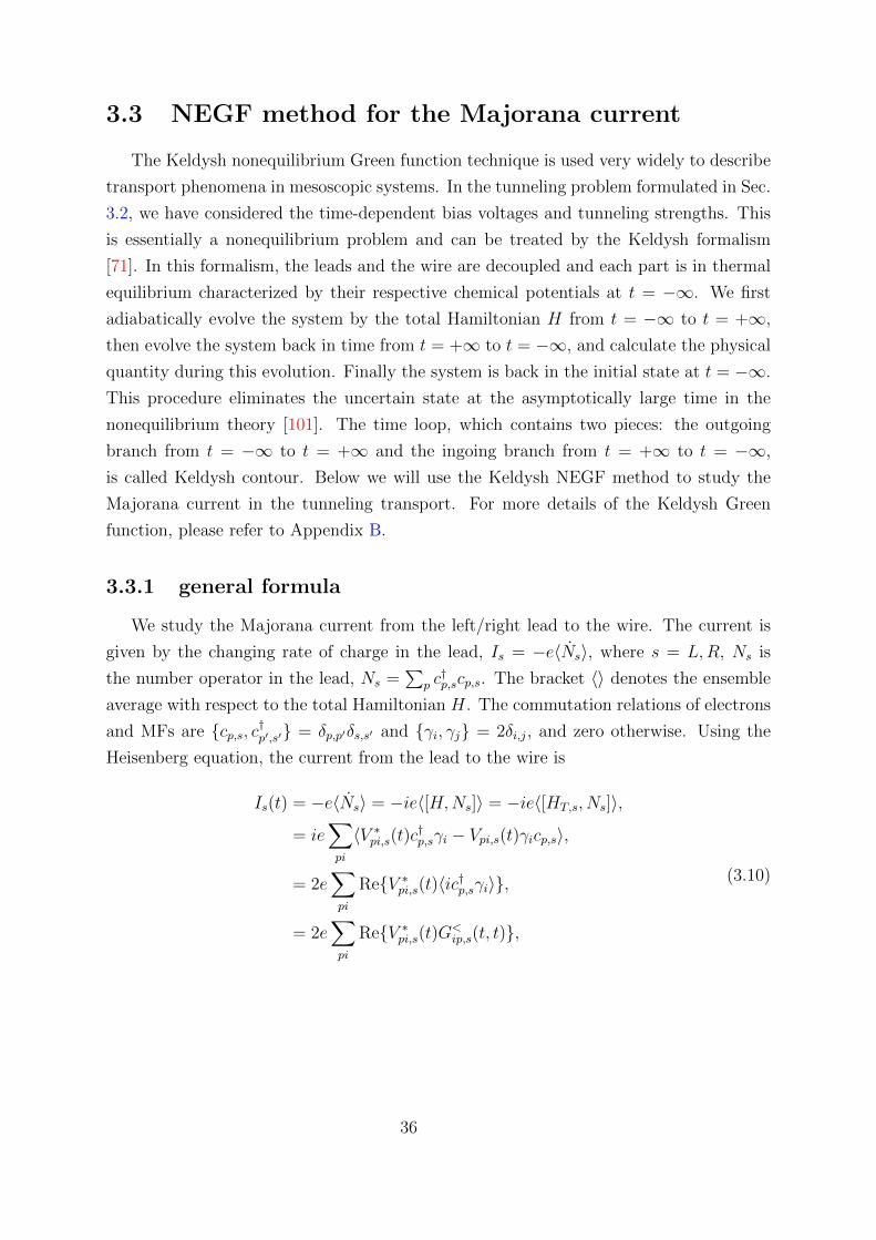
3.3 NEGF method for the Majorana current

The Keldysh nonequilibrium Green function technique is used very widely to describe

transport phenomena in mesoscopic systems. In the tunneling problem formulated in Sec.

3.2, we have considered the time-dependent bias voltages and tunneling strengths. This

is essentially a nonequilibrium problem and can be treated by the Keldysh formalism

[71]. In this formalism, the leads and the wire are decoupled and each part is in thermal

equilibrium characterized by their respective chemical potentials at t = −∞. We first

adiabatically evolve the system by the total Hamiltonian H from t = −∞ to t = +∞,

then evolve the system back in time from t = +∞ to t = −∞, and calculate the physical

quantity during this evolution. Finally the system is back in the initial state at t = −∞.

This procedure eliminates the uncertain state at the asymptotically large time in the

nonequilibrium theory [101]. The time loop, which contains two pieces: the outgoing

branch from t = −∞ to t = +∞ and the ingoing branch from t = +∞ to t = −∞,

is called Keldysh contour. Below we will use the Keldysh NEGF method to study the

Majorana current in the tunneling transport. For more details of the Keldysh Green

function, please refer to Appendix B.

3.3.1 general formula

We study the Majorana current from the left/right lead to the wire. The current is

given by the changing rate of charge in the lead, Is = −e〈Ns〉, where s = L,R, Ns is

the number operator in the lead, Ns =∑

p c†p,scp,s. The bracket 〈〉 denotes the ensemble

average with respect to the total Hamiltonian H. The commutation relations of electrons

and MFs are cp,s, c†p′,s′ = δp,p′δs,s′ and γi, γj = 2δi,j, and zero otherwise. Using the

Heisenberg equation, the current from the lead to the wire is

Is(t) = −e〈Ns〉 = −ie〈[H,Ns]〉 = −ie〈[HT,s, Ns]〉,

= ie∑pi

〈V ∗pi,s(t)c†p,sγi − Vpi,s(t)γicp,s〉,

= 2e∑pi

ReV ∗pi,s(t)〈ic†p,sγi〉,

= 2e∑pi

ReV ∗pi,s(t)G<ip,s(t, t),

(3.10)

36

where G<ip,s(t, t

′) = i〈c†p,s(t′)γi(t)〉 is the lesser component of the Keldysh Green function

Gip,s(t, t′) = −i〈TKγi(t)c†p,s(t′)〉. (3.11)

Here operator TK orders the times along the Keldysh contour with earlier times occurring

first.

To proceed, we express the coupling Green function Gip as a product of Green func-

tions for the lead Gp and the wire Gij. Via the equation of motion (EOM) method (see

Ref. [101] and Appendix C for details), we have

Gip,s(t, t′) =

∑j

ˆK

dt′′Gij(t, t′′)Vpj,s(t

′′)G0p,s(t

′′, t′), (3.12)

where

Gij(t, t′) = −i〈TKγi(t)γj(t′)〉,

G0p,s(t, t

′) = −i〈TKcp,s(t)c†p,s(t′)〉0(3.13)

are the Green function of the wire and the free Green function of the lead respectively.

Here 〈〉0 is the ensemble average with respect to the Hamiltonian of lead Hs. The in-

tegration is taken on the Keldysh contour. Therefore, via the Keldysh Green function

method [101], we can get the lesser component of the coupling Green function Eq. (3.12)

by analytic continuation (see Appendix B for details),

G<ip,s(t, t

′) =∑j

ˆ ∞−∞

dt′′Vpj,s(t′′)[GR

ij(t, t′′)G0<

p,s(t′′, t′) +G<

ij(t, t′′)G0A

p,s(t′′, t′)], (3.14)

where GR and GA are the retarded and advanced Green functions. The explicit expres-

sions for the free Green functions G0 can be found in Appendix D. Substituting this lesser

Green function into the current formula Eq. (3.10) and using the expressions for the free

Green functions, we arrive at

Is(t) =− 2eIm∑

ij

ˆ t

−∞dt1

ˆ ∞−∞

dε

2πeiε(t−t1)[Γs(ε, t1, t)]ji[G

Rij(t, t1)fs(ε) +G<

ij(t, t1)],

(3.15)

where fs(ε) is the Fermi function. The time-dependent level broadening matrix is given

37

by

[Γs(ε, t1, t)]ji = 2πρs(ε)V∗i,s(ε, t)Vj,s(ε, t1)e

−ie´ tt1dt2Us(t2)

, (3.16)

where the density operator is ρ(ε) =∑

p δ(ε − εp,s). Here we have explicitly indicated

the energy dependence of the tunneling strength Vpi,s(t). It is easy to check that the

broadening matrix is Hermitian, Γ†s(ε, t1, t) = Γs(ε, t, t1).

Since transport is often dominated by the states close to the Fermi level and the

broadening function is slowly varying function of energy, we apply the wide-band ap-

proximation [71] to the tunneling strength. The momentum and time dependence can

thus be factorized, Vpi,s(t) = Vi,s(εp,s, t) = us(t)Vi,s(εp,s). Thus we find that [Γs(t)]ji ≡[Γs(ε, t, t)]ji = [Γs(ε)]ji|us(t)|2, where the level broadening matrix is

[Γs(ε)]ji = 2πρs(ε)V∗i,s(ε)Vj,s(ε). (3.17)

Below we assume that the tunneling strength is time-independent and set us(t) = 1. In

the mesoscopic transport, the physical property is generally dominated by states near

the Fermi level. Since the broadening matrix is usually slowly varying function of energy

close to the Fermi level, we can assume that it is energy-independent, Γs(ε) = Γs. This

wide-band approximation captures the main physics of the tunneling problem and can

be used to simplify the current expression Eq. (3.15).

Therefore, the current can be further reduced to Is(t) = Iouts (t) + I in

s (t), where

Iouts (t) = −eImTr[ΓsG

<(t, t)],

I ins (t) = −eImTr

ˆ ∞−∞

dε

πfs(ε)

ˆ t

−∞dt1e

−iε(t1−t)Γs(t1, t)GR(t, t1)

.

(3.18)

Here Γs(t1, t) ≡ Γs(ε, t1, t) = Γse−ie´ tt1dt2Us(t2)

and G<,R are the Green functions of the

wire. The current has been separated in two parts: the outflow, Iouts (t), which is easy

to be identified since Γs represents the rate at which an electron placed initially in the

energy level of the wire will escape into the lead and N(t) = ImTr[G<(t, t)] is the number

of particles in the wire; the inflow, I ins (t), which is proportional to the occupation fs(ε)

in the lead and to the density of states ρ(ε) = ImTr[GR(ε)] in the wire. For the outflow,

the lesser Green function can be calculated by the relation [30]

G<(t, t) =

ˆdt1dt2G

R(t, t1)Σ<(t1, t2)GA(t2, t), (3.19)

38

where the explicit expression for the lesser self-energy Σ<(t1, t2) is given in Appendix C.

Substituting Σ< into the lesser Green function, we have

G<(t, t) =∑s=L,R

ˆdε

2π[ifs(ε)][As(ε, t)ΓsA

†s(ε, t) + Bs(ε, t)Γ

∗sB†s(ε, t)], (3.20)

where

As(ε, t) =

ˆdt1e

−iε(t1−t)eie´ t1t dt′Us(t′)GR(t, t1),

Bs(ε, t) =

ˆdt1e

−iε(t1−t)e−ie´ t1t dt′Us(t′)GR(t, t1).

(3.21)

Since Tr[ΓsAΓs′A†] is real, the outflow can be finally written as

Iouts (t) = −e

∑s′=L,R

ˆdε

2πfs′(ε)TrΓsAs′(ε, t)Γs′A

†s′(ε, t) + ΓsBs′(ε, t)Γ

∗s′B†s′(ε, t).

(3.22)

For the inflow, substituting Eq. (3.21) into Eq. (3.18), we obtain

I ins (t) = −e

ˆdε

πfs(ε)ImTrΓsAs(ε, t). (3.23)

The retarded Green function of the wire is deduced in Appendix C. Here we only show

the result,

GR(t, t1) = −2iθ(t− t1)e(2t−Γ)(t−t1), (3.24)

where θ(t) is the Heaviside step function. The level broadening matrix is Γ = 2(ΓL+ΓR),

where

ΓL =

[ΓL 0

0 0

],ΓR =

[0 0

0 ΓR

], (3.25)

and ΓL and ΓR are positive. The hopping matrix are

t =

[0 t

−t 0

]. (3.26)

39

3.3.2 dc current response

We first discuss the current response to the dc voltages at the two ends, UL(t) = UL

and UR(t) = UR. For the homogeneous system, As(ε, t) and Bs(ε, t) in Eq. (3.21)

are time-independent and just the Fourier transform of the retarded Green function,

As(ε, t) = GR(ε − eUs) and Bs(ε, t) = GR(ε + eUs). Substituting this relation into the

outflow Eq. (3.22), we immediately have

Iouts = −e

∑s′

ˆdε

2π[T ess′(ε)fs′(ε+ eUs′) + T hss′(ε)fs′(ε− eUs′)], (3.27)

where the particle and hole transmission functions are

T ess′(ε) = Tr[ΓsGR(ε)Γs′G

A(ε)],

T hss′(ε) = Tr[ΓsGR(ε)Γ∗s′G

A(ε)].(3.28)

Here the retarded Green function GR(ε) is the Fourier transform of Eq. (3.24) and can

be explicitly written as

GR(ε) =2[

ε+ 2iΓL −2it

2it ε+ 2iΓR

] ,(3.29)

and the advanced Green function is the Hermitian conjugation of the retarded one,

GA(ε) =2[

ε− 2iΓL −2it

2it ε− 2iΓR

] .(3.30)

Similarly, the inflow can be written as

I ins = −e

ˆdε

πfs(ε+ eUs)ImTrΓsG

R(ε),

= −eˆ

dε

2πifs(ε+ eUs)TrΓs[G

R(ε)−GA(ε)].(3.31)

Here we have used the fact that the retarded and advanced Green functions are con-

jugated. By the definitions of the retarded and advanced Green functions, we have

GR(ε)−GA(ε) = −i∑

s′ GR(ε)(Γs′+Γ∗s′)G

A(ε) [101]. Substituting this relation into the

40

inflow Eq. (3.31), we have

I ins = e

∑s′

ˆdε

2π[T ess′(ε)fs(ε+ eUs) + T hss′(ε)fs(ε+ eUs)]. (3.32)

Therefore, for the dc case, the current is reduced to the Landauer-Buttiker formula [30;

106],

Is = e∑s′

ˆdε

2πT ess′(ε)[fs(ε+ eUs)− fs′(ε+ eUs′)]

+ T hss′(ε)[fs(ε+ eUs)− fs′(ε− eUs′)].(3.33)

Here we encounter four transmission functions, T eLL, T eLR, T hLL and T hLR. The first one

injects an electron from the left lead and reflects an electron back to the left lead; this

process does not have contribution to the transport. The second one injects an electron

from the left lead and detects an electron at the right lead; this is the usual contribution

to the transport. The third one injects an electron from the left lead and reflects a hole

back to the left lead; this is the Andreev reflection of a superconductor. The fourth one

injects an electron from the left lead and detects a hole at the right lead; this is the

crossed Andreev reflection [63]. It is worth noting that due to the emergence of MFs

(γ = c + c†), there exists a hole transmission channel T hss′(ε) in Eq. (3.28) in Majorana

transport. This leads to the deviation from ordinary tunneling transport in the normal

nanowire [17; 106] and renders the left and right currents asymmetric, IL 6= −IR. For

example, when ΓL = ΓR = Γ, the quantity J = IL + IR is shown in Fig. 3.2. We observe

that only when UL = −UR (V = −2UL, where V = UR − UL), J is zero; otherwise,

J 6= 0 in the Γ ∼ V plane. It is easy to check that when the hole transmission function

T hss′ vanishes, the current symmetry is recovered, IL = −IR. This scenario happens in

the normal semiconducting nanowire [17; 106], the Anderson model [13; 143] and the

quantum dot systems [54; 154]. Therefore, the current asymmetry is a unique feature of

the Majorana transport in our two-lead setup and may be served as an indicator of the

emergence of the Majorana fermion.

We now investigate differential conductance of the Majorana nanowire at zero tem-

perature (βL/R = ∞). In the Majorana transport, we should define the current going

through the wire as I = 12(IL − IR). When the hole transmission function T hss′ = 0,

the definition reduces to the usual one. Without loss of generality, UL is fixed and we

calculate the conductance dI/dV ∼ V , where V = UR − UL. After some straightforward

41

Figure 3.2: Current asymmetry J = IL + IR in the Γ ∼ V plane ranging from −3 to+1.5. We set UL = 1 and ΓL = ΓR = Γ in this diagram.

calculations, we obtain that

dI

dV=

4e2

h

ΓLΓR(4t2 + 4ΓLΓR) + e2(V + UL)2Γ2R

[4t2 − e2(V + UL)2]2 + (4t2 + 4ΓLΓR)2 − (4t2)2 + 4e2(V + UL)2(Γ2L + Γ2

R).

(3.34)

Notice that when lead L decouples to the Majorana nanowire (ΓL = UL = 0), the

conductance reduces to the one in Ref. [42]. Interestingly, we observe that a critical line

ΓR = Γ3L/t

2 − 2ΓL separates the zero-bias conductance peak from zero-bias conductance

dip in the ΓR ∼ ΓL plane as shown in Fig. 3.3(a). For ΓL, there exists a critical value

ΓLc =√

2t, below which the zero-bias conductance always exhibits a dip as shown in

Fig. 3.3(b). Above this threshold, the zero-bias conductance undergoes a transition from

dip to peak as shown in Fig. 3.3(c). We also find that the ZBP becomes larger as the

level broadening is increased. The UL dependence of conductance is also shown in Fig.

3.3(d). It is easy to see that only when UL = 0, the peak is zero-bias, otherwise there is a

shift in the V direction. We also study the finite temperature effects as depicted in Fig.

3.3(e) and 3.3(f). As the temperature is increased, the scattering process occurs more

frequently, thereby leading to a reduction of the conductance. The competing effect of

voltage and temperature can be seen from the intersection of the conductance profiles

42

as well. Notice that even in the dip region of Fig. 3.3(a), the dip can become a peak

at zero-bias voltage as the temperature is increased as shown in Fig. 3.3(e). Although

the ZBP above is consistent with the Majorana interpretation, other mechanisms such as

impurity, disorder, [26; 126; 150] or zero-bias anomaly of Kondo physics [13; 54; 143; 154]

cannot be completely ruled out. In these cases, the currents at the left and right leads

remain symmetric, while in the two-lead tunneling transport involving Majorana fermion,

the currents are asymmetric. Therefore, the current asymmetry J can be served as an

auxiliary criterion for confirming the existence of Majorana fermion in the tunneling

experiment as depicted in Fig. 3.1.

3.3.3 ac current response

We turn to consider the current response to the ac voltages. The harmonic voltages

at the two ends of the nanowire are UL(t) = UL cosωLt and UR(t) = UR cos (ωRt+ φ)

respectively. When the voltage UR is enhanced, the current becomes less harmonic and

finally saturates at high voltage as shown in Fig. 3.4(a). The larger the level broadening

ΓR is, the stronger the coupling between lead and nanowire is. This leads to a higher

current response as shown in Fig. 3.4(b). In Fig. 3.4(c), we study the influence of

frequency difference of input signals at the left and right lead and find that a more

complicated periodic pattern appears. The effect of phase difference is given in Fig.

3.4(d). It is shown that the current response hits the peak when the two voltage signals

are out-of-phase. We also study the temperature effect in Fig. 3.4(e) and get similar

results as the dc case. The response to rectangular ac voltages are depicted in Fig.

3.4(f). The upper plane is the voltage signals and the lower plane is the current response.

It can be expected that in each plateau, the current response is the same as the dc case.

3.4 Interaction and disorder effects on the Majorana

transport

The interaction and disorder effects on the topological property of the wire are sig-

nificant. The disorder will destroy the transitional symmetry of the wire. We need to

43

0 1 2 3 40

2

4

6

8

10

GL

GR

HaLdip peak

GLc

-40 -20 0 20 400.0

0.2

0.4

0.6

0.8

1.0

V

dId

VHe2 h

L

HbL

-10 -5 0 5 100.0

0.2

0.4

0.6

0.8

V

dId

VHe2 h

L

HcL

-20 -10 0 10 200.0

0.2

0.4

0.6

0.8

V

dId

VHe2 h

L

HdL

-15 -10 -5 0 5 10 150.0

0.2

0.4

0.6

0.8

V

dId

VHe2 h

L

HeL

-15 -10 -5 0 5 10 150.0

0.2

0.4

0.6

0.8

V

dId

VHe2 h

L

HfL

Figure 3.3: Conductance for the dc voltage. We set t = 1 in all figures. (a) shows thecritical line for the dip-peak transition in the ΓR ∼ ΓL plane. The parameters in (b) areUL = 0, ΓL = 1 and ΓR = 1 (green dot-dashed), 3 (blue dashed), 5 (red solid); in (c) areUL = 0, ΓR = 1 and ΓL = 0.5 (green dot-dashed), 1.5 (blue dashed), 2.5 (red solid); in(d) are ΓL = 2, ΓR = 1 and UL = 5 (green dot-dashed), 0 (blue dashed), −5 (red solid);in (e) are UL = 0, ΓL = ΓR = 1 and βL = βR = 10 (green dot-dashed), 1.5 (blue dashed),0.5 (red solid); in (f) are UL = 0, ΓL = 2, ΓR = 1 and βL = βR = 10 (green dot-dashed),1 (blue dashed), 0.5 (red solid).

44

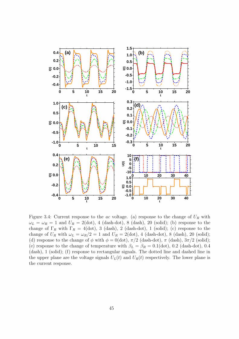
0 5 1 0 1 5 2 0- 0 . 4- 0 . 20 . 00 . 20 . 4 ( a )

I(t)

t0 5 1 0 1 5 2 0- 1 . 5

- 1 . 0- 0 . 50 . 00 . 51 . 01 . 5 ( b )

I(t)

t

0 5 1 0 1 5- 1 . 0- 0 . 50 . 00 . 51 . 0 ( c )

I(t)

t 0 5 1 0 1 5 2 0- 0 . 3- 0 . 2- 0 . 10 . 00 . 10 . 20 . 3 ( d )

I(t)

t

0 5 1 0 1 5 2 0- 0 . 4

- 0 . 2

0 . 0

0 . 2

0 . 4 ( e )

I(t)

t

0 1 0 2 0 3 0 4 0- 1 0- 505

1 0

0 1 0 2 0 3 0 4 0- 1 . 0- 0 . 50 . 00 . 51 . 0

U(t)

( f )

t

I(t)

Figure 3.4: Current response to the ac voltage. (a) response to the change of UR withωL = ωR = 1 and UR = 2(dot), 4 (dash-dot), 8 (dash), 20 (solid); (b) response to thechange of ΓR with ΓR = 4(dot), 3 (dash), 2 (dash-dot), 1 (solid); (c) response to thechange of UR with ωL = ωR/2 = 1 and UR = 2(dot), 4 (dash-dot), 8 (dash), 20 (solid);(d) response to the change of φ with φ = 0(dot), π/2 (dash-dot), π (dash), 3π/2 (solid);(e) response to the change of temperature with βL = βR = 0.1(dot), 0.2 (dash-dot), 0.4(dash), 1 (solid); (f) response to rectangular signals. The dotted line and dashed line inthe upper plane are the voltage signals UL(t) and UR(t) respectively. The lower plane isthe current response.

45

consider the Hamiltonian of the wire Eq. (3.1) in the real space,

H0 =

ˆdxφ†[− ∂2

x

2m− µ− i(ατy + βτx)∂x + Vzτz]φ,

H∆ = ∆

ˆdx(ψ↑ψ↓ + H.c.),

(3.35)

where φ = (ψ↑, ψ↓)T. We will use the bosonization method [20; 39; 52; 53; 96; 133] to

discuss the interaction and disorder effects in the wire. Generally, in one dimension, the

localization length due to the disorder is of the order of the mean free path. It means

that after bumping a couple of times on the impurities the electrons are localized [52]

and the wire becomes insulator. However, when the superconducting pairing satisfies

the condition Eq. (3.3), the wire is in the topological superconducting phase. This

competing mechanism can be quantitatively studied by the renormalization analysis of

the density-density correlation function of the wire.

3.4.1 brief introduction of bosonization

3.4.1.1 left and right movers representation

To obtain the low-energy properties of the wire, we can deal with excitations close to

the Fermi surface. Since the chemical potential µ lies within the gap, only the lower band

in Eq. (3.4) is activated, and for one dimension, there are only two Fermi points ±kF in

the energy spectrum. We can linearize the dispersion relation near each Fermi points. In

one dimension, because the low-energy particle-hole excitations have both well-defined

momentum and energy, this will lead to two species of fermions: left and right moving

fermions. We then replace the original model by the one where the energy spectrum is

purely linear. This is nothing but assuming that the density of states is constant [52].

To begin with, we write the field operator of the Hamiltonian in the left and right

movers representation. By the unitary transform aks =∑

ν〈s|χν(k)〉akν where s =↑, ↓and ν = ±, we can transform the field operator ψs(x) from the spin basis to the band

basis,

ψs(x) =1√2π

ˆdkeikxaks =

∑ν

1√2π

ˆdkeikx〈s|χν(k)〉akν . (3.36)

Because only the electrons with momentum k near two Fermi points ±kF of the lower

46

band in Eq. (3.4) are activated, we approximate the field operator as

ψs(x) ≈ 1√2π

ˆ −kF+Λ

−kF−Λ

dkeikx〈s|χ−(k)〉ak,− +1√2π

ˆ kF+Λ

kF−Λ

dkeikx〈s|χ−(k)〉ak,−,

≈ e−ikF x〈s|χ−(−kF )〉 1√2π

ˆ −kF+Λ

−kF−Λ

dkei(k+kF )xak,−

+ eikF x〈s|χ−(kF )〉 1√2π

ˆ kF+Λ

kF−Λ

dkei(k−kF )xak,−,

(3.37)

where Λ→ 0. Then we can express the field operator in terms of the left and right movers

as

ψs(x) =e−ikF x〈s|χ−(−kF )〉ψL(x) + eikF x〈s|χ−(kF )〉ψR(x), (3.38)

where the left and right movers are

ψL(x) =1√2π

ˆ ∞−∞

dkei(k+kF )xdk,L,

ψR(x) =1√2π

ˆ ∞−∞

dkei(k−kF )xdk,R.

(3.39)

Here dk,L and dk,R are the annihilation operators in the left and right branches of the

lower band and we have extended the linear dispersion relation to the whole Brillouin

zone by changing the range of integral for the left and right movers to (−∞,∞).

We now turn to study the kinetic term H0 in Eq. (3.5). By linearizing the energy

spectrum ε−(k) near the two Fermi point ±kF , the low energy kinetic term becomes

H0 ≈ˆ ∞−∞

dk[εF − νF (k + kF )]d†k,Ldk,L +

ˆ ∞−∞

dk[εF + νF (k − kF )]d†k,Rdk,R,

=

ˆ ∞−∞

dkνF (−k − kF )d†k,Ldk,L +

ˆ ∞−∞

dkνF (k − kF )d†k,Rdk,R + constant,

(3.40)

where εF =k2F

2m− µ −

√(α2 + β2)k2

F + V 2z and νF = kF

m− (α2+β2)kF√

(α2+β2)k2F+V 2

z

. On the other

47

hand, by the definition of ψR(x), we find that

ˆdxψ†R(x)(−iνF∂x)ψR(x)

=

ˆdkdk′

[1

2π

ˆdxei(k

′−k)x

]νF (k′ − kF )d†k,Rdk′,R,

=

ˆdkνF (k − kF )d†k,Rdk,R.

(3.41)

Therefore, the low energy kinetic term is

H0 = iνF

ˆdx[ψ†L(x)∂xψL(x)− ψ†R(x)∂xψR(x)]. (3.42)

Next we consider the s-wave superconducting term in Eq. (3.35). From Eq. (3.38), we

have

ψ↑(x)ψ↓(x)

=[e−ikF x(−e−iθ/2 sin

γ−kF2

)ψL(x) + eikF x(−e−iθ/2 sinγkF2

)ψR(x)]

·[e−ikF xeiθ/2 cos

γ−kF2

ψL(x) + eikF xeiθ/2 cosγkF2ψR(x)

],

= − sinγ−kF

2cos

γkF2ψL(x)ψR(x)− sin

γkF2

cosγ−kF

2ψR(x)ψL(x)

− e−i2kF x sinγ−kF

2cos

γ−kF2

ψL(x)ψL(x)− ei2kF x sinγkF2

cosγkF2ψR(x)ψR(x).

(3.43)

Neglecting the oscillating terms and taking into account that γ−k = arctan−√α2+β2k

Vz=

−γk, we find that

ψ↑(x)ψ↓(x) = sin γkFψL(x)ψR(x). (3.44)

Therefore, the s-wave superconducting term is

H∆ = ∆ sin γkF

ˆdx[ψL(x)ψR(x) + ψ†R(x)ψ†L(x)]. (3.45)

We next consider the Coulomb interaction which can be formulated as

Hint =

ˆdxdx′V (x− x′)ρ(x)ρ(x′), (3.46)

where the electron density operator is ρ(x) =∑

s=↑,↓ ψ†s(x)ψs(x). In the momentum

48

space, the interaction can be recast into

Hint =1

2Ω

∑k,s,k′,s′,q

V (q)a†k+q,sa†k′−q,s′ak′,s′ak,s. (3.47)

Similarly, we transform the Hamiltonian to the band basis (ak+, ak−) and neglect the

upper-band operators, then the interaction term becomes

Hint =1

2Ω

∑k,k′,q

V (q) cosγk+q − γk

2cos

γk′−q − γk′2

d†k+qd†k′−qdk′dk. (3.48)

One should be reminded that the most efficient processes in the interaction are the ones

that can act close to the Fermi surface. Particularly in one dimension, it is worth noting

that the Fermi surface is reduced to two points ±kF that allow us to decompose the

interaction into three scattering processes. The first one is exchange scattering, where two

electrons moving in the same direction collide and exchange their velocities; the second

one is forward scattering, where two electrons moving in the opposite directions collide

and keep moving in their original directions; the third one is the backward scattering,

where two electrons moving in the opposite directions collide and move backward. Notice

that the wave vector q for the forward and exchange processes is ∼ 0, and ∼ ±2kF for the

backward scattering. It is easy to see that the forward and backward scattering processes

are identical for the spinless fermion as the particles are indiscernible. Therefore, the

interaction Hamiltonian can be expressed as the sum of the above scattering processes:

Hint =V (0)

2Ω

∑k∈R,k′∈R,q∼0

d†k+qd†k′−qdk′dk +

V (0)

Ω

∑k∈R,k′∈L,q∼0

d†k+qd†k′−qdk′dk + (R↔ L).

(3.49)

Using the definitions of the left and right movers Eq. (3.39), the interaction can be

written as

Hint = g2

ˆdxψ†R(x)ψR(x)ψ†L(x)ψL(x)

+g4

2

ˆdxψ†R(x)ψR(x)ψ†R(x)ψR(x)

+g4

2

ˆdxψ†L(x)ψL(x)ψ†L(x)ψL(x),

(3.50)

where g2/2 = g4 = V (0). Now we turn to study the disorder term. When the impurities

49

are weak and dense enough so that the effect of each impurity is negligible, they can only

act collectively. In this case, there are many impurities in a volume small compared to the

scale of variation of the physical quantities but large compared to the distance between

impurities. Physically it means that one can replace the original disorder by a coarse

grained version. This coarse grained disorder is equivalent to a Gaussian disorder [52]

due to the central limit theorem. The disorder potential U(x) can be treated as a random

chemical potential on the impurity sites. Thus the disorder term can be formulated as

Hdis =

ˆdxU(x)ρ(x), (3.51)

where the disorder potential satisfies Gaussian distribution

p(U) = exp[− 1

2D

ˆdxU2(x)

]. (3.52)

Here we assume that the impurity potential is short-range so that 〈U(x)U(x′)〉 = Dδ(x−x′). Fourier transforming the Hamiltonian and projecting it onto the lower band, we have

Hdis =1

Ω

∑k,q

U(q) cosγk+q − γk

2d†k+qdk. (3.53)

Again, the most important processes are the ones close to the Fermi surface. In one

dimension, the disorder term can be thus approximated as

Hdis =1

Ω

∑q∼0

U(q)∑k∼±kF

d†k+qdk

+cos γkF

Ω

∑q∼2kF

U(q)∑k∼−kF

d†k+qdk

+cos γkF

Ω

∑q∼−2kF

U(q)∑k∼kF

d†k+qdk.

(3.54)

In the left and right movers representation, we have

Hdis =

ˆdxη(x)[ψ†R(x)ψR(x) + ψ†L(x)ψL(x)]

+ cos γkF

ˆdx[ξ(x)ψ†L(x)ψR(x) + ξ∗(x)ψ†R(x)ψL(x)],

(3.55)

where η(x) = 1Ω

∑q∼0 U(q)eiqx and ξ(x) = 1

Ω

∑q∼0 U(q − 2kF )eiqx are two independent

50

Gaussian random variables. Note that η(x) is real and ξ(x) is complex. The correlation

relations are 〈η(x)η(x′)〉 = 〈ξ(x)ξ∗(x′)〉 = Dδ(x− x′), and zero otherwise.

3.4.1.2 bosonization of the Majorana nanowire

The Abelian bosonization formula [48; 52; 96; 97] is given by

ψL(x) =1√2πα

e−i√

4πφL(x),

ψR(x) =1√2πα

ei√

4πφR(x),(3.56)

where ψL/R(x) is the massless Dirac field (fermionic) as shown in Eq. (3.39), and φL/R(x)

is massless Klein-Gordon field (bosonic). α is the short-range cutoff for the convergence

of the continuum theory. Please see Appendix E for details.

Using the formula Eq. (3.56), the kinetic energy Eq. (3.42) can be bosonized as

H0 = πνF

ˆdx[ρ2

L(x) + ρ2R(x)], (3.57)

where ρL/R(x) = 1√π∂xφL/R(x) is the normal-ordered density operator for left/right mover.

Please see Appendix F for the bosonization of the kinetic energy Eq. (3.57). We define

two new variables, φL = −1√4π

(θ+ϕ) and φR = 1√4π

(θ−ϕ), where the commutation relation

is [θ(x), ϕ(y)] = iπsgn(y − x)/2. The Hamiltonian H0 then becomes

H0 =νF2π

ˆdx[(∂xθ)

2 + (∂xϕ)2]. (3.58)

For the s-wave superconducting term, substituting Eq. (3.56) into Eq. (3.45), after

bosonization it can be written as

H∆ =∆ sin γkF

πα

ˆdx cos 2θ. (3.59)

Similarly, the Coulomb interaction Eq. (3.50) in terms of the field θ and ϕ is

Hint =g2

4π2

ˆdx[(∂xϕ)2 − (∂xθ)

2] +g4

4π2

ˆdx[(∂xϕ)2 + (∂xθ)

2]. (3.60)

The bosonic form of the disorder term Eq. (3.55) is given by

Hdis = − 1

π

ˆdx[η(x)∂xϕ] +

cos γkF2πα

ˆdx[ξ(x)e−i2ϕ + ξ∗(x)ei2ϕ]. (3.61)

51

Notice that in one dimension, the effect of Coulomb interaction just leads to the repa-

rameterization of the kinetic energy H0. The interaction can be absorbed into the kinetic

energy, then we arrive at the following Hamiltonian for the Luttinger liquid,

HLutt = H0 +Hint =1

2π

ˆdx[uK(∂xθ)

2 +u

K(∂xϕ)2

], (3.62)

where the Luttinger parameters are

u = νF[(1 + y4)2 − y2

2

]1/2,

K =

(1 + y4 − y2

1 + y4 + y2

)1/2

.(3.63)

Here y2 = g2

2πνFand y4 = g4

2πνF. Furthermore, we observe that the first term in Eq.

(3.61) is equivalent to a random gauge potential which can also be absorbed into the

Hamiltonian of Luttinger liquid Eq. (3.62) via replacing ϕ(x) by ϕ(x) − Ku

´ xdyη(y).

Finally, we achieve the bosonic Hamiltonian of the interacting wire with Gaussian disorder

Hdw = HsG +Hbws, where

HsG =1

2π

ˆdx[uK(∂xθ)

2 +u

K(∂xϕ)2

]+

∆ sin γkFπα

ˆdx cos 2θ,

Hbws =cos γkF

2πα

ˆdx[ξ(x)e−i2ϕ + ξ∗(x)ei2ϕ].

(3.64)

The Hamiltonian HsG is the well-known sine-Gordon Hamiltonian which has Kosterlitz-

Thouless phase transition [84]. The superconducting term favors a superconducting

ground state, however, the disorder term tends to pin the charge density to the dis-

order potential and favors an insulator phase [97]. Therefore, we can expect the disorder

system undergoes a topological phase transition as the interplay of superconductivity and

disorder.

3.4.2 influence on the Majorana transport

In general, we can use the perturbation theory to calculate the correlation function,

for instance,

R(r1 − r2) = 〈eia√

2ϕ(r1)e−ia√

2ϕ(r2)〉Hdw, (3.65)

52

to study the physical property of the interacting disorder wire [52]. The average for a

system with a disorder potential U can be treated by the replica method as follows,

〈O(ϕ)〉Hdw= lim

n→0

´D[ξ, ξ∗]p(ξ, ξ∗)

´ n∏i=1

DϕiO(ϕ1)e−

n∑a=1

SU (θa,ϕa)

´D[ξ, ξ∗]p(ξ, ξ∗)

,(3.66)

where O(ϕ) is some observable of ϕ. Please see Appendix G for details. Basically, we

need to perform the functional integral over the n-copies of replicas ϕi and the Gaussian

distributed random variables ξ and ξ∗. The Gaussian distributed disorder potential is

p(ξ, ξ∗) = e−1D

´dxξ(x)ξ∗(x) and the action of the disorder system can be achieved by the

Legendre transformation of the Hamiltonian Hdw,

SU(θa, ϕa) = −ˆ β

0

dτ

ˆdx

i

π∂xθ∂τϕ+

ˆ β

0

dτHdw. (3.67)

By integrating out the Gaussian random variables ξ and ξ∗, we arrive at

〈O(ϕ)〉Hdw= lim

n→0

ˆ n∏i=1

DϕiO(ϕ1)e−Seff , (3.68)

where

Seff =n∑a=1

[S0(ϕa) + S∆(ϕa)]−D cos2 γkF

(2πα)2

n∑a,b=1

ˆdxdτdτ ′ cos [2ϕa(x, τ)− 2ϕb(x, τ

′)].

(3.69)

Here S0 = −´ β

0dτ´dx i

π∂xθ∂τϕ +

´ β0dτHLutt and S∆ =

´ β0dτH∆. The details of cal-

culation of correlation function Eq. (3.65) by the replica method Eq. (3.68) is given

in Appendix H. After some calculations, we find that the perturbation result is plagued

by divergence which is notorious in one dimension. However, although the correlation is

infinite, it should be independent of the change of short-range cutoff α because it char-

acterizes the physical properties of the system. This peculiar property suggests the use

of the renormalization group method [52; 97]. Particularly, by expanding the supercon-

ducting and disorder actions to the first leading order, changing the short-range cutoff

α → αel and keeping the correlation function unchanged (see Appendix H for details),

53

-4 -3 -2 -1 0-4

-3

-2

-1

0

ln@yDHlLD

ln@y

DHlL

D

HaL

TSC

NTI

-4 -3 -2 -1 0-4

-3

-2

-1

0

ln@yDHlLD

ln@y

DHlL

D

HbLKH0L=0.7KH0L=0.9KH0L=1.1KH0L=1.3

Figure 3.5: (a) RG flows of yD(l) and y∆(l), where K(0) = 1.2. NTI and TSC are short fornon-topological insulator and topological superconductor. The orange line is the phaseboundary. (b) phase boundaries with different K(0)s.

we obtain the RG flows as follows,

dK/dl = y2∆ − yDK2,

dy∆/dl = (2−K−1)y∆,

dyD/dl = 2Ky2D − (2K − 3 + 2K−1y2

∆)yD,

du/dl = −yDKu,

(3.70)

where y∆ = α∆ sin γkF /u and yD = αD cos2 γkF /πu2. From the flows of y∆(l) and yD(l),

we can see that when K(l) < 1/2, yD(l) is relevant, the system is in the random-pinned

change density wave phase; when K(l) > 3/2, y∆(l) is relevant, the system is in the

superconducting phase. When 1/2 < K(l) < 3/2, both yD(l) and y∆(l) are relevant. In

order to be consistent with the perturbation condition, the flows can be chosen to stop

at l∗ when max [yD(l∗), y∆(l∗)] = 1. Using this criterion, the phase diagram in this K(l)

interval is obtained as shown in Fig. 3.5(a). Only when the parameters are in the shadow

region, the Majorana fermions remain. In Fig. 3.5(b), we plot the phase boundaries

with respect to different initial K(0) and find that the topological superconducting phase

becomes larger as K(0) increases. Therefore, when K(l) < 1/2 or when 1/2 < K(l) < 3/2

as well as the parameters are in the shadow region of Fig. 3.5(a), y∆ is relevant and

the Majorana transport is preserved, otherwise the disorder strength D will destroy the

transport.

54

Part II

Mott-superfluid transition in hybrid

circuit-QED system

55

Chapter 4

Phase transition of light in

circuit-QED lattices coupled to

nitrogen-vacancy centers in diamond

4.1 Introduction

The microscopic properties of strongly correlated many-particle systems emerging in

solid-state physics are in general very hard to access experimentally [56; 60; 61]. So

a method to simulate the properties of condensed-matter models using non-traditional

controllable systems is highly desirable. Recently, the investigation of quantum simulation

in photon-based many-body physics has received much attention in different systems

[41; 56; 60; 61; 82; 136; 137]. Especially, there has been great interest in mimicking

the quantum phase transition (QPT) of light by a scalable coupled resonator array in

the context of cavity/circuit quantum electrodynamics (QED) [22; 50; 65; 73; 93; 124;

160; 167], which provides a convenient controllable platform for studying the strongly

correlated states of light via photonic processes. On the other hand, artificially engineered

hybrid devices can permit measurement access with good experimental control [38; 94];

and it is intriguing to employ a highly controllable quantum system with a tunable

Hamiltonian to simulate the physics of another system of interest. This paradigm has

promoted many experimental/theoretical proposals on probing the light phase and opened

various possibilities for the simulation of many-body physics.

In this chapter, we elaborate an optical system for engineering the strongly correlated

effects of light in a hybrid solid-state system. We consider a two-dimensional (2D) square

56

lattice of coupled transmission line resonators (TLRs) [10; 25; 140], where each TLR is

coupled to a single nitrogen vacancy (NV) [21; 35; 47; 68; 174] encircled by a persistent

current qubit (PCQ). We show that the competition between the on-site TLR-PCQ in-

teraction and the nonlocal hopping induces the photonic localization-delocalization tran-

sition. Subsequently the Mott insulator (MI) phase and the superfluid (SF) phase can

appear in a controllable way. The phase boundary in the case of photon hopping with

real/complex-valued amplitudes can be obtained using the mean-field approach. Also, the

quantum jump technique is employed to describe the phase diagram when the dissipation

is considered. Finally, the possibility of observation of the QPT is discussed.

In our architecture, one can tune independently the on-site TLR-PCQ interaction and

the nonlocal photonic hopping between adjacent TLRs. This permits us to systematically

study the localization-delocalization transition of light in a complete parameter space.

The main motivation for building such a hybrid system is to combine several advantages:

in situ tunability of circuit elements [15; 112; 168], transmission measurement for state

readout [10], peculiar characteristics of NVs (e.g., individual addressing [15; 87] and

long coherence time at room-temperature [2; 72; 115]), and scalability of TLR arrays

[34; 55; 65; 81; 103; 114; 118]. Due to the easy readout of the states of NV by laser or

microwave, it is possible to indirectly probe the quantum many body states of our hybrid

system by NV center. Recently, Underwood et al experimentally fabricated 25 arrays of

TLRs and demonstrated the feasibility of quantum simulation in a circuit-QED system

[153]. Lucero et al experimentally fabricated a complex circuit composed of four phase

qubits and five TLRs to realize intricate quantum algorithms [98]. The progress renders

the TLR lattice as a good platform for studying condensed-matter physics with photons

and makes our scheme more practical.

The main results of this chapter were published in the following paper:

• Jia-Bin You, W. L. Yang, Zhen-Yu Xu, A. H. Chan, and C. H. Oh, Phase transition

of light in circuit-QED lattices coupled to nitrogen-vacancy centers in diamond.

Physical Review B 90, 195112 (2014).

4.2 Model

As illustrated in Fig. 4.1, we consider a 2D lattice of coupled TLRs, where the basic

unit consists of a TLR coupled to a single NV encircled by a PCQ, which acts as an

interconnect to greatly magnify the NV-TLR coupling by several orders of magnitude,

57

compared with the direct NV-TLR coupling (far below the linewidth of TLR by dozens

of KHz) resulting from the vacuum fluctuations of the photons [1; 152].

The TLR is made of a superconductor line interrupted by two capacitors at its ends.

In the microwave domain, it can be treated as a quantum LC harmonic oscillator,

HTLR = ωr(a†a+ 1/2), (4.1)

where a (a†) is the annihilation (creation) operator of the photonic mode in the TLR, and

ωr =√

1/LrCr is the corresponding eigenfrequency with inductance Lr and capacitance

Cr. Here we set ~ = 1. The PCQ located at an antinode of the TLR’s magnetic field

is formed by a superconducting loop interrupted by three Josephson junctions, where all

the junctions are identical except that one is smaller than the other two as shown in Fig.

4.1 [120; 152]. When the loop is biased by half a magnetic flux quantum, the device is

an effective two-level qubit made up of two countercirculating persistent currents. This

effective two-level system is described by the Hamiltonian HPCQ = 12(εσz + ∆0σx), where

σx and σz are the Pauli matrices. Here ε = 2Ip(Φ − Φ0/2), where Ip is the persistent

circulating current of the PCQ loop, Φ is the external magnetic flux through the loop

induced by the current in the central conductor of the TLR and Φ0 is the flux quantum;

∆0 is the coupling between the two states of the two-level PCQ system [152]. Going to

the eigenbasis we can write this two-level system as

HPCQ =ω0

2σz, (4.2)

where ω0 =√ε2 + ∆2

0. The NV can be modeled as a three-level system in the triplet

ground-state subspace consisting of |3A,ms = 0〉 and |3A,ms = ±1〉. The Hamiltonian is

HNV = γeBzSz +D(S2z − 2/3), (4.3)

where γe is the electronic gyromagnetic ratio, D/2π ∼ 2.87 GHz is the zero-field split-

ting which is predominantly due to dipolar spin-spin coupling between the two unpaired

electrons forming the NV center, Bz is a perpendicular magnetic field at the NV cen-

ter induced by the persistent circulating current and Sz = diag1, 0,−1 is the spin-1-z

operator.

The PCQ magnetically couples to the TLR via mutual inductance, HT-P = −µ · B,

where µ is the magnetic dipole of PCQ induced by the persistent circulating currents and

58

B is the magnetic field at the PCQ induced by the current in the central conductor of

the TLR. To quantize the Hamiltonian, the magnetic field is taken to consist of a single

bosonic mode with the field operator B ∼ a† + a and the PCQ is coupled to the field

through its magnetic dipole µ ∼ σ+ + σ−, where σ± = 12(σx ± iσy). Moving the TLR-

PCQ coupling to interaction picture, we have HT-P ∼ ei(ωr+ω0)ta†σ+ + e−i(ωr+ω0)taσ− +

ei(ωr−ω0)ta†σ−+ e−i(ωr−ω0)taσ+. When ωr ∼ ω0, the counter-rotating terms a†σ+ and aσ−

can be safely ignored by means of the rotating wave approximation. Therefore, we arrive

at the famous Jaynes-Cummings (JC) type interaction

HT-P = g(a†σ− + aσ+), (4.4)

where g = (Ipµ0r2/d)

√ωr/2Lr. Here r is the radius of the PCQ loop, d is the distance

between the PCQ and central conductor of the TLR, and µ0 is Bohr magneton. The

changes of magnetic flux within the loop induced by Ip presented in the PCQ lead to

small shifts in the transition frequencies (ms → ±1) of the NV [120; 152]. Through this

small change in magnetic field the PCQ can couple to the NV via the Zeeman term,

HN-P =1

2ησzSz, (4.5)

where the coupling is η = Ipµ0γe/r.

Therefore, the basic unit of our system at site p is thus governed by the Hamiltonian

H0p = HTLR + HPCQ + HNV + HT-P + HN-P. To get the eigenstates of the Hamiltonian

H0p , we note that [H0

p , Sz] = 0, thus Sz can be replaced by its eigenvalue ms. We then

consider a sector of the Hamiltonian labeling by ms,

H0p (ms) = ωr(a

†a+ 1/2) + (ω0 + ηms)σz/2 + g(a†σ− + aσ+) + χ(ms), (4.6)

where Sz|ms〉 = ms|ms〉 and χ(ms) = γeBzms + D(m2s − 2/3) is the eigenenergy of

HNV. Furthermore, the Hamiltonian can be written as a sum of two commuting parts,

H0p (ms)− χ(ms) = HI +HII , where

HI = ωr(a†a+ 1/2 + σz/2),

HII = (−∆ + ηms)σz/2 + g(a†σ− + aσ+).(4.7)

Here the detuning between the TLR and the PCQ is ∆ = ωr − ω0. The eigenstates of

59

HI , being of tensor product form, can be easily solved and denoted by

|n, g〉 =

(a†)n

√n!|0〉 ⊗

[0

1

],

|n, e〉 =

(a†)n

√n!|0〉 ⊗

[1

0

],

(4.8)

where n is the number of microwave photons in a single TLR, |g〉 and |e〉 are the ground

and excited states of the two-level PCQ system. Via this observation and taking HII into

account, it is enough to diagonalize the Hamiltonian H0p (ms) in the subspaces spanned

by |n, e〉, |n+ 1, g〉. The Hamiltonian projected into this subspaces is

h0p(ms) =

[〈n, e|H0

p (ms)|n, e〉 〈n, e|H0p (ms)|n+ 1, g〉

〈n+ 1, g|H0p (ms)|n, e〉 〈n+ 1, g|H0

p (ms)|n+ 1, g〉

]. (4.9)

Since

H0p (ms)|n, e〉 = [(n+ 1/2)ωr + (ω0 + ηms)/2 + χ(ms)]|n, e〉+ g

√n+ 1|n+ 1, g〉,

H0p (ms)|n+ 1, g〉 = [(n+ 3/2)ωr − (ω0 + ηms)/2 + χ(ms)]|n+ 1, g〉+ g

√n+ 1|n, e〉,

(4.10)

the Hamiltonian h0p(ms) can be explicitly written as[

(n+ 1/2)ωr + (ω0 + ηms)/2 + χ(ms) g√n+ 1

g√n+ 1 (n+ 3/2)ωr − (ω0 + ηms)/2 + χ(ms)

].

(4.11)

Therefore, diagonalizing the Hamiltonian Eq. (4.11) via the eigenequation |EI−h0p(ms)| =

0, where E is the eigenenergy and I is the identical matrix, the photon-dependent eigenen-

ergies can be obtained,

E±(n) = (n+ 1)ωr ± Ωn(∆)/2 + χ(ms), (4.12)

where the Rabi frequency is Ωn(∆) =√

4g2(n+ 1) + (∆− ηms)2. The corresponding

60

Figure 4.1: (a) Schematic circuit for the resonator lattice, where each TLR is coupled toa single NV center encircled by a PCQ, and the red circles denote the central coupler.(b) The subsystem consisting of NV and PCQ, where NV is at the center of the loop.The PCQ is made up of three Josephson junctions, and it couples to the NV via themagnetic field at the center of the loop generated by the persistent currents in the loop.The energy levels of NV are shown in the red box.

eigenstates are

|n,+〉 = sinβn2|n, e〉+ cos

βn2|n+ 1, g〉,

|n,−〉 = − cosβn2|n, e〉+ sin

βn2|n+ 1, g〉,

(4.13)

where tan βn = 2g√n+1

∆−ηms . Therefore, the eigenststes of the whole HamiltonianH0p , |ms, n,±〉

= |ms〉 ⊗ |n,±〉, which consist of a microwave photon at TLR, an excitation mode from

PCQ and an excitation mode from NV are called dressed states (polariton). The unper-

turbed TLR eigenstates |n〉 are modified (dressed) by the interaction with the PCQ and

the NV, and their eigenfrequencies are shifted by the Rabi frequency.

We present a paradigm for a 2D TLR lattice coupled to the solid-state spins of the NV

centers. We have shown that a specially engineered resonator lattice provides a practical

platform to couple both individual spin and superconducting qubit, and engineer their

interactions in a controllable way.

61

4.3 Mott-superfluid transition

We study the full Hamiltonian of the 2D square lattice by adding the on-site chemical

potential and the nonlocal microwave photonic tunneling between adjacent sites. Here

the photonic tunneling in our model can be realized by a central coupler which serves as

an individual tunable quantum transducer to transfer photonic states between adjacent

TLRs. Here, the central coupler may be conceived as a Josephson ring circuit [55; 81; 118],

or a current-biased Josephson junction phase qubit [11; 105; 171; 172], or a capacitive

coupling element [67], or an active nonreciprocal device as proposed in Ref. [75]. The

Hamiltonian is given by

H =∑p

H0p +

∑〈p,q〉

k〈p,q〉a†paq −

∑p

µpNp, (4.14)

where µp is the chemical potential at site p, ap (a†p) is the annihilation (creation) operator

of the photonic mode in the TLR at site p, and k〈p,q〉 = 2Z0C〈p,q〉(ωr + δp)(ωr + δq)

are photonic tunneling rates between two adjacent resonators p and q denoted by 〈p, q〉,which are set by the tunable mutual capacitance C〈p,q〉 between resonator ends with

characteristic impedance Z0 and frequency shift δp due to random disorder [153]. Since

ωr δp, one can assume that k〈p,q〉 = k = 2Z0Cω2r without disorder for nearest-neighbor

resonators, and k〈p,q〉 = 0 for other resonator pairs. Here we have tuned the mutual

capacitance C〈p,q〉 = C for all the photonic tunneling between two adjacent TLRs. The

conserved quantity in our system is the total number of polaritons N =∑

p(a†pap +

σ+p σ−p + 1

2S+p S−p ) with Si (σi) the spin-1 (-1/2) operators (i = ±). Thus we can define

the chemical potential µp for polaritons at site p.

The photon-dependent eigenstates of the Hamiltonian H0p are dressed states |ms,±, n〉

with the eigenenergies Eq. (4.12). The interaction of this hybrid system H0p is governed by

the JC-type of coupling Eq. (4.4), which enables the interconversion of qubit excitations

and photons, and provides the effective on-site repulsion. This effective on-site repulsion

can be defined as the energy cost of adding an additional polariton into a lattice site [56].

Here we study the zero-temperature property of the Hamiltonian, thus only the lower

energy band of Eq. (4.12) is considered. Therefore, the on-site repulsion is given by

U(n) = |E|ms,−,n+1〉 − E|ms,−,n〉 − ωr|. Meanwhile, the microwave photon in the TLR can

tunnel from one TLR to its neighboring TLRs. This competition between the effective on-

site repulsion and the nearest neighbor photon hopping will lead to the Mott-superfluid

transition. The difference between the Bose-Hubbard model [85] and our model is that

62

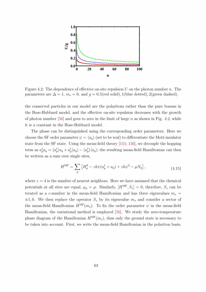
0 20 40 60 80 1000.0

0.2

0.4

0.6

0.8

1.0

n

Ug

Figure 4.2: The dependence of effective on-site repulsion U on the photon number n. Theparameters are ∆ = 1, ms = 0, and g = 0.5(red solid), 1(blue dotted), 2(green dashed).

the conserved particles in our model are the polaritons rather than the pure bosons in

the Bose-Hubbard model, and the effective on-site repulsion decreases with the growth

of photon number [56] and goes to zero in the limit of large n as shown in Fig. 4.2, while

it is a constant in the Bose-Hubbard model.

The phase can be distinguished using the corresponding order parameters. Here we

choose the SF order parameter ψ = 〈ap〉 (set to be real) to differentiate the Mott-insulator

state from the SF state. Using the mean-field theory [155; 156], we decouple the hopping

term as a†paq = 〈a†p〉aq + a†p〈aq〉 − 〈a†p〉〈aq〉; the resulting mean-field Hamiltonian can then

be written as a sum over single sites,

HMF =∑p

[H0p − zkψ(a†p + ap) + zkψ2 − µNp

], (4.15)

where z = 4 is the number of nearest neighbors. Here we have assumed that the chemical

potentials at all sites are equal, µp = µ. Similarly, [HMF, Sz] = 0, therefore, Sz can be

treated as a c-number in the mean-field Hamiltonian and has three eigenvalues ms =

±1, 0. We then replace the operator Sz by its eigenvalue ms and consider a sector of

the mean-field Hamiltonian HMF(ms). To fix the order parameter ψ in the mean-field

Hamiltonian, the variational method is employed [56]. We study the zero-temperature

phase diagram of the Hamiltonian HMF(ms), thus only the ground state is necessary to

be taken into account. First, we write the mean-field Hamiltonian in the polariton basis,

63

10-4 10-3 10-2 10-1 100 101-3.0-2.7-2.4-2.1-1.8-1.5-1.2-0.9-0.6-0.30.0

10-4 10-3 10-2 10-1 100 101-4.0-3.6-3.2-2.8-2.4-2.0-1.6-1.2-0.8-0.40.0

10-4 10-3 10-2 10-1 100 101-2.0-1.8-1.6-1.4-1.2-1.0-0.8-0.6-0.4-0.20.0

10-4 10-3 10-2 10-1 100 101-3.0-2.7-2.4-2.1-1.8-1.5-1.2-0.9-0.6-0.30.0

(a)

(d)

10-4 10-3 10-2 10-1 100 101-4.0-3.6-3.2-2.8-2.4-2.0-1.6-1.2-0.8-0.40.0

k/g

k/gk/g

k/g

(b)

(e)

10-4 10-3 10-2 10-1 100 101-2.0-1.8-1.6-1.4-1.2-1.0-0.8-0.6-0.4-0.20.0

k/g

(c)

0

1

2

3

4

(-

r)/g

(-

r)/g

(-

r)/g

(-

r)/g

(-

r)/g

(f)

(-

r)/g

k/g

Figure 4.3: The phase diagrams in the µ ∼ k plane for different sets of NV-PCQ coupling ηand tunable magnetic fields Bz applied on a NV, where µ and k are the chemical potentialand the photon hopping rate. The common parameters are g = 1, ωr = 200, D = 100,and γe = −103. The other parameters are set as follows: (a) η = 0.01, Bz = 0.0005T,and ∆ = g; the phase boundaries are plotted in (d), where ∆ = 2g (solid), g (dashed),and 0 (dot-dashed). (b) η = 1.2, Bz = −0.3T, and ∆ = 0; the phase boundaries areplotted in (e), where Bz = −0.3T (solid), 0.0005T (dashed), and 0.3T (dot-dashed). (c)η = 0.75, Bz = 0.3T, and ∆ = 0; the phase boundaries are plotted in (f), where η = 0.01(solid), η = 0.75 (dashed), and η = 1.5 (dot-dashed).

64

|g, 0〉, |e, 0〉, |g, 1〉, |e, 1〉, |g, 2〉, |e, 2〉, · · ·. In this basis, HMF (ms) reads

−ω0

2− ηms

20 −zkψ 0 0 0

0 ω0

2+ ηms

2− µ g −zkψ 0 0

−zkψ g ωr − ω0

2− ηms

2− µ 0 −

√2zkψ 0

0 −zkψ 0 ωr + ω0

2+ ηms

2− 2µ

√2g −

√2zkψ

0 0 −√

2zkψ√

2g 2ωr − ω0

2− ηms

2− 2µ 0 · · ·

0 0 0 −√

2zkψ 0 2ωr + ω0

2+ ηms

2− 3µ · · ·

· · · · · · · · ·

+

[ωr2

+ γeBzms +D(m2s −

2

3) + zkψ2 − µ(1 +

ms

2− m2

s

2)

]I.

(4.16)

We then truncate HMF (ms) at a finite value of n photon states, nmax. Second, numerically

diagonalize this Hamiltonian in the truncated basis and identify the ground state energy,

Eg. Third, increase nmax until Eg converges to its value at nmax =∞. Finally, minimize

Eg with respect to ψ for different values of µ and k. The order parameter can then be

fixed by ψ(µ, k) : ∂Eg(µ, k)/∂ψ = 0. We plot ψ in the (µ, k) plane to obtain the mean-

field phase diagram/boundary when η varies from the weak coupling regime (η g) to

the strong coupling regime (η > g) under the resonant/detuning case. The features of

Fig. 4.3 are rich. The regime where ψ = 0 corresponds to the stable and incompressible

MI lobes characterized by a fixed number of excitations per site with no variance. In each

MI lobe, due to the nonlinearity and anharmonicity in the spectrum originating from the

photon blockade effect [9; 64; 89], the strong TLR-PCQ interaction leads to an effective

large polariton-polariton repulsion which freezes out hopping and localizes polaritons at

individual lattice sites. By contrast, strong hopping favors delocalization and leads to a

condensation of the particles into the zero-momentum state; namely, ψ 6= 0 indicates a SF

compressible phase with the stable ground state at each site corresponding to a coherent

state of excitations. The compressibility is defined as the changeability of the average

number of polaritons per site in the grand canonical ensemble, ρ = −∂Eg(ψ = ψmin)/∂µ.

When ∂ρ/∂µ = 0, the system has constant density and is incompressible; otherwise the

system is compressible [56].

Analogous to the Bose-Hubbard model, the underlying physical picture is that the MI-

SF phase transition results from the interplay between polariton delocalization and on-site

repulsive interaction. Therefore, the phase boundary primarily depends on the ratio of

the photon-hopping k to the on-site repulsion. When the on-site repulsion dominates

over hopping, the system is in the MI phase, otherwise the system is in the SF phase.

From the expressions of the parameter η and g, we can find that reduction of the size

of the PCQ loop will increase η but decrease g, and the adjustment of the distance d

65

only affects the TLR-PCQ interaction. Furthermore, the detuning ∆ is also tunable by

varying the magnetic field applied on the NV. In Fig. 4.3, one can find that the size of

the MI lobes varies with ∆.

Further insight into the transition can be gained when the photonic hopping with

complex-valued amplitude exists in Eq. (4.14), where the hopping process becomes

−∑〈p,q〉

k〈p,q〉eiφ〈p,q〉a†paq with tunneling phase φ〈p,q〉 = −φ〈q,p〉 and we set k〈p,q〉 = k. We

emphasize that this process is possible if the intermediate coupling elements break time-

reversal symmetry [55; 65; 81; 118; 121]. It can be realized by the passive coupling

elements. By the meaning of passive, the coupler only transfers photons via interme-

diate virtual excitations and otherwise remains in its ground state at all times. Conse-

quently, the coupler degrees of freedom can be integrated out so that the effective hopping

for the passive coupling elements becomes complex. The complex tunneling amplitude

k〈p,q〉eiφ〈p,q〉 provides a new perspective in the dynamical evolution of the system. Con-

sider the case where the tunneling phases inside each row/column of the TLR lattice in

Fig. 4.1 are equal, and the phases in all the rows/columns are in an alternate pattern of

2πα,−2πα, 2πα,−2πα, · · ·, then in the mean-field approximation, the hopping term

becomes

−∑〈p,q〉

k〈p,q〉eiφ〈p,q〉a†paq = −

∑〈p,q〉

keiφ〈p,q〉a†paq,

= −k∑p

(ei2παa†p+xap + ei2παa†p+yap + H.c.),

=∑p

[−zkψ cos (2πα)(a†p + ap) + zkψ2 cos (2πα)],

(4.17)

where x (y) is the unit vector in the x (y) direction. Here we have applied the mean-field

approximation in the third line of Eq. (4.17). Therefore, the total Hamiltonian under

the mean-field approximation reads

HMFα =

∑p

[H0p − zkψ cos(2πα)(a†p + ap) + zkψ2 cos(2πα)− µNp

]. (4.18)

The phase diagram is exhibited in Fig. 4.4; we find that the boundary line gradually

shifts to the right as α increases in the interval [0, 1/4]. Because of the spatial variation

of the tunneling phase, the wave function of a polariton from one lattice site to another

acquires a nontrivial phase, which actually reduces the effective hopping rates from k to

k cos (2πα).

66

10-4 10-3 10-2 10-1 100 101-2.0-1.8-1.6-1.4-1.2-1.0-0.8-0.6-0.4-0.20.0

10-4 10-3 10-2 10-1 100 101-2.0-1.8-1.6-1.4-1.2-1.0-0.8-0.6-0.4-0.20.0

(a)

0

1

2

3

4

(-

r)/g

k/g

(b)

(-

r)/g

k/g

Figure 4.4: (a) The order parameter ψ in the µ ∼ k plane. The parameters are g = 1,ωr = 200, D = 100, γe = −103, η = 0.01, Bz = 0.0005T, α = 0.2, and ∆ = 0. Thecorresponding phase boundaries are plotted in (b), where the solid, dashed, and dot-dashed line denote α = 0, 0.2, and 0.24, respectively.

4.4 Dissipative effects

Generally, nonequilibrium processes such as the dissipative effect, are crucial in solid-

state devices. We show that the signature of the Mott-superfluid transition remains

even in the presence of the engineered dissipation by the quantum trajectory method

[16; 123] (see Appendix I for details). By this approach, the non-Hermitian Hamiltonian

is formulated as

Hdiss = HMF − iΓ

2

∑p

σ+p σ−p −

iκ

2

∑p

a†pap, (4.19)

where κ is the decay rate of the TLR, and Γ is the decay rate from the effective excited

state |e〉 to the ground state |g〉 of the PCQ. In our case, the dissipative effects result

from the unavoidable interaction between the PCQ/TLR and the corresponding Marko-

vian environment; for example, the interaction between the output of the TLR and the

corresponding vacuum field will result in photon escape into the environment. Here the

dissipative effects of the NV are negligible, compared with κ and Γ. The phase diagrams

under dissipative effects are displayed in Fig. 4.5. Once the hopping rate is increased

beyond a critical value, the system is expected to undergo a nonequilibrium QPT from

a MI phase, where the initial photon population imbalance between two resonators is

self-trapped, to a SF phase where it coherently oscillates between the two TLRs [65].

Furthermore, another obvious feature is that the size of the MI phase becomes larger

with the growth of dissipative rates. Note that the effective on-site repulsion becomes

67

10-4 10-3 10-2 10-1 100 101-2.0-1.8-1.6-1.4-1.2-1.0-0.8-0.6-0.4-0.20.0

k/gk/g

(a)

10-4 10-3 10-2 10-1 100 101-2.0-1.8-1.6-1.4-1.2-1.0-0.8-0.6-0.4-0.20.0

(b)

10-4 10-3 10-2 10-1 100 101-2.0-1.8-1.6-1.4-1.2-1.0-0.8-0.6-0.4-0.20.0

k/gk/g

(c)10-4 10-3 10-2 10-1 100 101

-2.0-1.8-1.6-1.4-1.2-1.0-0.8-0.6-0.4-0.20.0

(-

r)/g

(-

r)/g

(-

r)/g

(-

r)/g

(d)

0

1

2

3

4

Figure 4.5: The order parameter ψ in the µ ∼ k plane under different dissipative rates:(a) Γ = κ = 0.01, (b) Γ = κ = 0.05, (c) Γ = κ = 0.1, and (d) Γ = κ = 0.15. The otherparameters are g = 1, ωr = 200, D = 100, γe = −103, η = 0.01, Bz = 0.0005T, and∆ = 0.

stronger at lower excitation number as depicted in Fig. 4.2, which implies that the dis-

sipative effect (inducing the decrease of the excitation number) favors the MI phase. As

a result, the dissipation results in the dynamical switching from SF phase to MI phase

and causes the enlargement of the size of MI phase.

4.5 Experimental feasibility

We briefly stress the relevant experimental progress. On one hand, it is possible to

fabricate large arrays to observe many-body physics of interacting polaritons since res-

onators and qubits can be made lithographically [151]. Actually, it is indeed feasible

to couple over 200 TLRs with negligible disorders (on the order of a few parts in 104)

in a 2D lattice using a 32mm×32mm sample. This number can easily be extended to

more than 1000 TLRs on a full two-inch wafer [65]. On the other hand, how to probe

quantum many-body states of polaritons is still an open question in photonic quantum

simulation [102]. The previous works suggested measuring the individual TLR through

mapping the excitations into the qubit followed by obtaining the state-selective resonance

fluorescence spectrum [5; 60; 61], but a remaining technical challenge is the realization

68

of high-efficiency photon detectors. Alternatively, the local statistical property of the

TLR can be analyzed readily using combined techniques of photon-number-dependent

qubit transition [74; 141] and fast readout of the qubit state through a separate low-

Q resonator mode [92], for which the high-efficiency photon detectors are not required.

Experimentally, transmission and reflection measurements for circuit-QED arrays have

been implemented successfully in small systems with one or two resonators [22; 74; 160].

In order to distinguish between different phases of the system, one can also experimen-

tally probe beyond transmission, such as by two-tone spectroscopy and a second-order

coherence function (photon statistics) to reveal additional information [43; 144; 149]. For

instance, by driving a TLR with a microwave source and detecting the output field of the

other TLR, we could probe the properties of the system by independently detecting the

correlation between two remote sites. The tunability of coupling strengths in our system

enables one to measure these quantities relative straightforwardly.

Finally, we survey the relevant experimental parameters. Given the flexibility of

circuit-QED, we can access a wide range of tunable experimental parameters for TLR-

PCQ coupling strength g and hopping rate k〈p,q〉. Taking Lr = 2nH, ωr/2π = 6 GHz,

Ip = 600nA, and r = 0.2µm, we get η/2π ≈ 140KHz and g/2π ≈ [1.8, 180]MHz when the

distance d varies from 5µm to 50nm. In Ref. [153], the authors measured devices with

photon hopping rates k/2π from 0.8 to 31 MHz in resonator lattices. The electron-spin

relaxation time T1 of the NV ranges from 6 ms at room temperature [116] to 28-265 s at

low temperature [59]. In addition, later experimental progress [6] with isotopically pure

diamond has demonstrated a longer dephasing time to be T2 = 1.8ms. Therefore, the

dissipation and decoherence of the NV are negligible.

69

Chapter 5

Summary and outlook

In Chapter 2, we investigate the topological phase and the Majorana bound state in the

spin-singlet superconductor with Rashba and Dresselhaus (110) spin-orbit couplings. In

Sec. 2.4, we find that there exist flat Andreev bound states which host Majorana fermions

in the s-wave Dresselhaus (110) superconductor. In Sec. 2.5, we study the topological

properties of the spin-orbit coupled spin-singlet superconductor. Due to the particle-hole

symmetry of the BdG Hamiltonian, we can use the Pfaffian invariant P to demonstrate

all the possible phase diagrams of the spin-singlet superconductor with Rashba and Dres-

selhaus (110) spin-orbit couplings. We find that only when the Hamiltonian has partial

particle-hole symmetry or chiral symmetry, the edge spectrum is Majorana flat band

protected by the edge index, namely, one dimensional Pfaffian invariant P(ky) or the

winding number W(ky); otherwise the edge spectrum is Dirac cone. These edge indices

can be used in determining the location of the zero-energy Majorana flat bands. The

Majorana flat band implies a peak in the density of states which is clearly visible and

can be detected in the transport measurements [7; 28; 109; 127; 164].

In Chapter 3, we use the Keldysh formalism to comprehensively study the two-lead

tunneling in Majorana nanowire with and without short-range Coulomb interaction and

disorder. A zero-bias dc conductance peak appears in our layout which implies the exis-

tence of Majorana fermion and is consistent with previous experiments on InSb nanowire

[23; 27; 31; 40; 91; 109]. We find that since the Majorana fermion is a fermion that is

its own antiparticle, there exists a hole transmission channel which makes the currents

asymmetric at the left and right leads. This current asymmetry may be used as a criterion

for detecting the Majorana fermion in our two-lead setup as depicted in Fig. 3.1. For

the ac voltage, we find that the current response is enhanced in step with the increase of

level broadening and the decrease of temperature, and finally saturates at high voltage.

70

The effects of short-range Coulomb interaction and disorder to the Majorana transport

have been considered via bosonization method and renormalization group analysis. We

find that there is a topological phase transition in the interplay of superconductivity and

disorder. In the topological superconducting phase, the Majorana transport remains,

otherwise the transport will destroy in the non-topological insulator phase.

In Chapter 4, we devise a concrete hybrid system to engineer a photonic Mott-

superfluid phase transition in a 2D square lattice of TLRs coupled to a single NV encircled

by a PCQ. We find that the interplay between the on-site repulsion and the photon tun-

neling leads to the photonic localization-delocalization transition (MI-SF transition). In

the presence of dissipation, the phase diagram can be obtained by the mean-field ap-

proach and the quantum trajectory method. Facilitated by the good connectivity in

circuit-QED, experiments combining both scalability and long coherence times are ex-

pected in the coming few years; at that stage the investigation of photonic quantum phase

transition using TLR lattice systems can be realized.

We now discuss possible future research directions. For Part I, it is interesting to

apply the recursive Green function method to explore the transport property of different

kinds of junctions involving topological insulator, topological superconductor, ferromag-

net, quantum dot and so on [18; 49; 78; 95; 157; 162]. We would like to study the

influence of these junctions on the zero-bias conductance peak which is a signal of Ma-

jorana fermion. Meanwhile, we can also study the effects of magnetic field, interaction,

Kondo impurity, disorder and geometry of device on the transport. For Part II, it is in-

teresting to study simulations of many body physics by the cavity-QED and circuit-QED

systems [22; 50; 65; 73; 93; 111; 117; 124; 160; 167]. For example, we would like to study

simulation of the fractional quantum Hall effect by the cavity or circuit QED system [62].

71

Appendix A

Edge spectra of topological

superconductor with mixed

spin-singlet pairings

The superconductors with mixed s-wave and d-wave pairing symmetries are of the case

(a), (f) and (g) in Tab. 2.1. For each case, there are three different kinds of phase diagrams

depending on the hopping amplitude t as demonstrated in Fig. 2.5(b)-2.5(d). Although

the edge spectrum becomes more complicated, there are no qualitative differences in

the edge spectrum between the d + s-wave superconductor and the pure d-wave or s-

wave superconductor. The edge spectra for the dx2−y2 + s-wave superconductor with

Dresselhaus (110) spin-orbit coupling are shown in Fig. A.1. Due to the partial particle-

hole symmetry and the chiral symmetry, the edge spectra of this kind of superconductor

are Majorana flat bands protected by the Pfaffian invariant P(ky) and the winding number

W(ky). Notice that in Fig. A.1(f) and Fig. A.1(t), the winding number W(ky) in some

range of ky is 2, however, its parity namely the Pfaffian invariant P(ky) is 1. Therefore,

the phase is trivial in this range of ky. The edge spectra for the dx2−y2 + idxy + s-wave

superconductor with Rashba/Dresselhaus (110) spin-orbit coupling are shown in Fig. A.2

and Fig. A.3 respectively. Without protection of the partial particle-hole symmetry or

the chiral symmetry, the Majorana flat bands disappear and become Dirac cones. In the

nontrivial topological phase, we find that the edge spectra have an odd number of Dirac

cones.

72

Figure A.1: (a)-(e) and (k)-(o) are the edge spectra of the dx2−y2 +s-wave superconductorwith Dresselhaus (110) spin-orbit coupling in case (f) of Tab. 2.1. There are three differentkinds of phase diagrams depending on the hopping amplitude t as shown in Fig. 2.5(b)-2.5(d). For the phase diagram of Fig. 2.5(b), the edge spectra are demonstrated in (a),(b) and (c). The parameters are t = 2, β = 1, ∆s1 = 1, ∆d1 = 2 and (a) µ = 0, V 2 = 16,(b) µ = −2.5, V 2 = 36, (c) µ = −4, V 2 = 20, which correspond to regions I, II and III inFig. 2.5(b) respectively. (f), (g) and (h) are the Pfaffian invariant and winding number for(a), (b) and (c). For the phase diagram of Fig. 2.5(c), the edge spectra are demonstratedin (d), (e), (k) and (l). The parameters are t = 1, β = 1, ∆s1 = 1, ∆d1 = 2 and (d)µ = 0, V 2 = 12, (e) µ = 0, V 2 = 20, (k) µ = −1.8, V 2 = 30, (l) µ = −4.5, V 2 = 25, whichcorrespond to regions I, II, III and IV in Fig. 2.5(c) respectively. (i), (j), (p) and (q) arethe Pfaffian invariant and winding number for (d), (e), (k) and (l). For the phase diagramof Fig. 2.5(d), the edge spectra are demonstrated in (m), (n) and (o). The parametersare t = 0.5, β = 1, ∆s1 = 1, ∆d1 = 2 and (m) µ = 0, V 2 = 16, (n) µ = −7, V 2 = 81, (o)µ = −1, V 2 = 5, which correspond to regions I, II and III in Fig. 2.5(d) respectively. (r),(s) and (t) are the Pfaffian invariant and winding number for (m), (n) and (o).

73

Figure A.2: (a)-(j) are the edge spectra of the dx2−y2 + idxy +s-wave superconductor withRashba spin-orbit coupling in case (a) of Tab. 2.1. For the phase diagram of Fig. 2.5(b),the edge spectra are demonstrated in (a), (b) and (c). The parameters are t = 2, α = 1,∆s1 = 1, ∆s2 = 0, ∆d1 = 2, ∆d2 = 1 and (a) µ = 0, Vz = 4, (b) µ = −2.5, Vz = 6, (c)µ = −4, Vz = 2

√5, which correspond to regions I, II and III in Fig. 2.5(b) respectively.

For the phase diagram of Fig. 2.5(c), the edge spectra are demonstrated in (d), (e), (f)and (g). The parameters are t = 1, α = 1, ∆s1 = 1, ∆s2 = 0, ∆d1 = 2, ∆d2 = 1 and (d)µ = 0, Vz = 2

√3, (e) µ = 0, Vz = 2

√5, (f) µ = −1.8, Vz =

√30, (g) µ = −4.5, Vz = 5,

which correspond to regions I, II, III and IV in Fig. 2.5(c) respectively. For the phasediagram of Fig. 2.5(d), the edge spectra are demonstrated in (h), (i) and (j). Theparameters are t = 0.5, α = 1, ∆s1 = 1, ∆s2 = 0, ∆d1 = 2, ∆d2 = 1 and (h) µ = 0, Vz = 4,(i) µ = −7, Vz = 9, (j) µ = −3, Vz = 3, which correspond to regions I, II and III in Fig.2.5(d) respectively.

74

Figure A.3: (a)-(j) are the edge spectra of the dx2−y2 + idxy +s-wave superconductor withDresselhaus (110) spin-orbit coupling in case (g) of Tab. 2.1. For the phase diagramof Fig. 2.5(b), the edge spectra are demonstrated in (a), (b) and (c). The parametersare t = 2, β = 1, ∆s1 = 1, ∆s2 = 0, ∆d1 = 2, ∆d2 = 1 and (a) µ = 0, V 2 = 16, (b)µ = −2.5, V 2 = 36, (c) µ = −4, V 2 = 20, which correspond to regions I, II and IIIin Fig. 2.5(b) respectively. For the phase diagram of Fig. 2.5(c), the edge spectra aredemonstrated in (d), (e), (f) and (g). The parameters are t = 1, β = 1, ∆s1 = 1, ∆s2 = 0,∆d1 = 2, ∆d2 = 1 and (d) µ = 0, V 2 = 12, (e) µ = 0, V 2 = 20, (f) µ = −1.8, V 2 = 30,(g) µ = −4.5, V 2 = 25, which correspond to regions I, II, III and IV in Fig. 2.5(c)respectively. For the phase diagram of Fig. 2.5(d), the edge spectra are demonstrated in(h), (i) and (j). The parameters are t = 0.5, β = 1, ∆s1 = 1, ∆s2 = 0, ∆d1 = 2, ∆d2 = 1and (h) µ = 0, V 2 = 16, (i) µ = −7, V 2 = 81, (j) µ = −1, V 2 = 5, which correspond toregions I, II and III in Fig. 2.5(d) respectively.

75

Appendix B

Keldysh non-equilibrium Green

function

The kernel of equilibrium many-body theory is the time-ordered Green function given

by

Gc(t, t′) = −i〈Ψ0|TψH(t)ψ†H(t′)|Ψ0〉

〈Ψ0|Ψ0〉, (B.1)

where T is the time-ordered operator, ψH(t) is the field operator in the Heisenberg picture

and Ψ0 is the ground state of the full Hamiltonian. Here the full Hamiltonian can be

divided into two parts, H = H0 +V , where H0 is the non-interacting part of the Hamilto-

nian in which the ground state Φ0 can be easily obtained, and V is the interacting part of

the Hamiltonian. However, the exact ground state Ψ0 of the Hamiltonian H is generally

hard to be acquired. To make any progress, we can express the exact ground state Ψ0

in terms of quantities we know, for example the non-interacting ground state Φ0. These

two states are related by the S-matrix as given in the Gell-Mann and Low theorem [101]:

|Ψ0〉 = S(0,−∞)|Φ0〉. (B.2)

We have introduced the S-matrix which changes the wavefunction from ψ(t′) to ψ(t):

ψ(t) = S(t, t′)ψ(t′). Therefore the traditional argument is that one starts in the remote

past (t = −∞) with the ground state ψ(−∞) = Φ0 of the non-interacting Hamiltonian

H0. The operator S(0,−∞) brings this wave function adiabatically up to the present

t = 0. We now have the ground state ψ(0) = Ψ0 which contains the effects of the

76

interaction V , so that it is an eigenstate of H. In equilibrium, one possible and reasonable

assumption is that as t → +∞, ψ(∞) = S(∞, 0)Ψ0 is equal to Φ0 except for a phase

factor. Therefore, the equilibrium time-ordered Green function can be rewritten as

Gc(t, t′) = −i〈Φ0|TS(∞,−∞)ψH(t)ψ†H(t′)|Φ0〉

〈Φ0|S(∞,−∞)|Φ0〉. (B.3)

Starting from this formula, the diagrammatic technique for calculating the equilibrium

Green function perturbatively can be developed [101].

However, because in the non-equilibrium problem the irreversible effects break the

symmetry between t = −∞ and t = +∞, the initial state at t = −∞ is generally different

from the final state at t = +∞. This makes the assumption in equilibrium problem where

the initial and final states are equal up to a phase factor invalid. Therefore, we cannot

define the non-equilibrium Green function by virtue of Eq. (B.3).

For non-equilibrium problem, one can abandon this assumption by first evolving the

Hamiltonian from t = −∞ to the moment of interest τ , and then continuously evolving

the Hamiltonian back in time from τ to t = −∞. The advantage of this so-called

Keldysh formalism is that one starts and ends with a known state ψ(−∞) = Φ0 which

is the eigenstate of H0 and is usually the only state we knows exactly. In this formalism

one can define the Keldysh Green function as follows:

G(t, t′) = −i〈Φ0|TKS(−∞,−∞)ψH(t)ψ†H(t′)|Φ0〉〈Φ0|S(−∞,−∞)|Φ0〉

, (B.4)

where TK is the contour-ordered operator on the time loop as shown in Fig. B.1(a). This

Keldysh contour contains two pieces: the outgoing branch L1 from t = −∞ to t = +∞and the ingoing branch L2 from t = +∞ to t = −∞. The S-matrix, S(−∞,−∞)

should be interpreted in the contour-ordered sense [101]. With this definition Eq. (B.4),

the contour-ordered Green function contains four different functions as shown in Fig.

B.1(b)-(e),

G(t, t′) =

Gc(t, t′) t, t′ ∈ L1

G>(t, t′) t ∈ L2, t′ ∈ L1

G<(t, t′) t ∈ L1, t′ ∈ L2

Gc(t, t′) t, t′ ∈ L2

, (B.5)

where Gc(t, t′) is the usual time-ordered Green function, Gc(t, t

′) is the anti-time-ordered

77

t

cG cG

GG

't

't

t

1L

2L

(a)

(b) (c)

(d) (e)

Figure B.1: the Keldysh contour (a) and the Keldysh Green function (b)-(e).

Green function, G>(t, t′) is the greater Green function and G<(t, t′) is the lesser Green

function.

Next we study the analytic continuation of the Keldysh Green function. The main

technical trick needed in the analytic continuation is Langreth Theorem. Considering the

following product,

A(t, t′) =

ˆL

dτB(t, τ)C(τ, t′), (B.6)

where L is the Keldysh contour. The lesser Green function is then given by

A<(t, t′) =

ˆL1

dτB(t, τ)C<(τ, t′) +

ˆL2

dτB<(t, τ)C(τ, t′), (B.7)

where L1 and L2 are the outgoing and ingoing branches of the Keldysh contour L. Con-

sidering the first term and splitting the integral into two parts, we have

ˆL1

dτB(t, τ)C<(τ, t′)

=

ˆ t

−∞dt1B

>(t, t1)C<(t1, t′) +

ˆ −∞t

dt1B<(t, t1)C<(t1, t

′),

=

ˆ ∞−∞

dt1θ(t− t1)(B>(t, t1)−B<(t, t1))C<(t1, t′),

=

ˆ ∞−∞

dt1BR(t, t1)C<(t1, t

′),

(B.8)

78

where BR(t, t1) is the retarded Green function. Similarly, we have

ˆL2

dτB(t, τ)C<(τ, t′) =

ˆ ∞−∞

dt1B<(t, t1)CA(t1, t

′), (B.9)

where CA(t1, t′) is the advanced Green function. Finally, we arrive at

A<(t, t′) =

ˆ ∞−∞

dt1[BR(t, t1)C<(t1, t′) +B<(t, t1)CA(t1, t

′)]. (B.10)

Similarly, for the greater Green function, we have

A>(t, t′) =

ˆ ∞−∞

dt1[BR(t, t1)C>(t1, t′) +B>(t, t1)CA(t1, t

′)]. (B.11)

Usually, one also needs the retarded (or advanced) component of a product of Green

functions defined on the Keldysh contour. We first express the retarded Green function

in terms of the lesser and greater Green function [101],

AR(t, t′) = θ(t− t′)[A>(t, t′)− A<(t, t′)], (B.12)

then substituting the definitions of lesser and greater Green functions Eq. (B.10) and

Eq. (B.11) into Eq. (B.12), we have

AR(t, t′) =

ˆ t

t′dt1B

R(t, t1)CR(t1, t′). (B.13)

Similarly, the analytic continuation of the greater Green function is

AA(t, t′) =

ˆ t′

t

dt1BA(t, t1)CA(t1, t

′). (B.14)

79

Appendix C

Green function and self-energy for

Majorana nanowire

Here we use the equation of motion method to study the Green function of the wire.

The Keldysh Green function for the nanowire is defined as Gij(t, t′) = −i〈TKγi(t)γj(t′)〉.

We first consider the time evolution of this Green function. By definition

Gij(t, t′) = −iθ(t− t′)〈γi(t)γj(t′)〉+ iθ(t′ − t)〈γj(t′)γi(t)〉, (C.1)

where θ(t− t′) is defined on the Keldysh contour. Then we have

∂tGij(t, t′) = −2iδ(t− t′)δi,j − i〈TK∂tγi(t)γj(t′)〉. (C.2)

Using the Heisenberg equation i∂tγk(t) = [γk(t), H], where H is the Hamiltonian of the

system, it is easy to check that the time evolution of Majorana operator is

i∂tγk(t) = −2i∑i

tikγi(t)−∑

p,s=L,R

2(V ∗pk,sc†p,s(t)− Vpk,scp,s(t)). (C.3)

Substituting Eq. (C.3) into Eq. (C.2), after some calculations we have

i∂tGij(t, t′) = 2δ(t− t′)δi,j + 2i

∑k

tikGkj(t, t′)

+ 2∑

p,s=L,R

(Vpi,sGpj,s(t, t′)− V ∗pi,sGpj,s(t, t

′)),(C.4)

80

where the Green function for the tunnelings are given by

Gpj,s(t, t′) = −i〈TKcp,s(t)γj(t′)〉,

Gpj,s(t, t′) = −i〈TKc†p,s(t)γj(t′)〉.

(C.5)

Similarly, we can use the equation of motion method [101] to express these two

tunneling Green functions in terms of the wire Green function. for example, we have

(i∂t − ξp,s)Gpj,s(t, t′) =

∑i V∗pi,sGij(t, t

′) which leads to the following closed form for

Gpj,s(t, t′),

Gpj,s(t, t′) =

∑i

ˆdt′′G0

p(t, t′′)V ∗pi,sGij(t

′′, t′), (C.6)

and similarly,

Gpj,s(t, t′) = −

∑i

ˆdt′′G

0

p(t, t′′)Vpi,sGij(t

′′, t′), (C.7)

where the free lead Green function is defined as

G0p(t, t

′) = −i〈TKcp(t)c†p(t′)〉0,

G0

p(t, t′) = −i〈TKc†p(t)cp(t′)〉0.

(C.8)

It is easy to check that the free lead Green functions satisfy the point charge source

equation,

(i∂t − ξp,L)G0p(t, t

′) = δ(t− t′),

(i∂t + ξp,L)G0

p(t, t′) = δ(t− t′),

(C.9)

which lead to the closed forms for Gpj,s(t, t′) and Gpj,s(t, t

′) respectively.

Therefore, substituting Eq. (C.6) and Eq. (C.7) into Eq. (C.4), we have

i∂tGij(t, t′) = 2δ(t− t′)δi,j + 2i

∑k

tikGkj(t, t′)

+ 2∑

k,s=L,R

ˆdt′′Σik,s(t, t

′′)Gkj(t′′, t′),

(C.10)

81

where the self-energy is Σs = Σes + Σh

s . The electron and hole self-energies are given by

Σeik,s(t, t

′′) =∑p

Vpi,s(t)G0p,s(t, t

′′)V ∗pk,s(t′′),

Σhik,s(t, t

′′) =∑p

Vpk,s(t)G0

p,s(t, t′′)V ∗pi,s(t

′′).(C.11)

We now study the retarded component of the self-energy ΣRik = ΣeR

ik,L + ΣeRik,R + ΣhR

ik,L +

ΣhRik,R, where

ΣeRik,s(t, t

′′) =∑p

Vpi,s(t)G0Rp,s(t, t

′′)V ∗pk,s(t′′),

ΣhRik,s(t, t

′′) =∑p

V ∗pi,s(t)G0R

p,s(t, t′′)Vpk,s(t

′′).(C.12)

By the wide-band approximation, the retarded self-energy is

ΣeRik,s(t, t

′′) =

ˆdε

2π[Γs]ikG

0Rp,s(t, t

′′). (C.13)

Substituting the free retarded Green function in Appendix D into Eq. (C.13), the retarded

self-energy for electron becomes

ΣeRs (t, t′′) = − i

2Γs(t)δ(t− t′′). (C.14)

Similarly, the retarded self-energy for hole is

ΣhRs (t, t′′) = − i

2Γ∗s(t)δ(t− t′′). (C.15)

Therefore, the retarded self-energy for the Majorana nanowire is

ΣR(t, t′′) = − i2Γ(t)δ(t− t′′), (C.16)

where Γ(t) = ΓL(t) + ΓR(t) + Γ∗L(t) + Γ∗R(t). Finally, by the analytic continuation [101]

of Eq. (C.10), we have

i∂tGRij(t, t

′) = 2δ(t− t′)δij + 2i∑k

tikGRkj(t, t

′) + 2∑k

ˆdt′′ΣR

ik(t, t′′)GR

kj(t′′, t′). (C.17)

Substituting Eq. (C.16) into it, we arrive at [i∂t−2it+ iΓ(t)]GR(t, t′) = 2δ(t− t′), which

82

leads to the solution to the retarded Green function

GR(t, t′) = −2iθ(t− t′)e´ tt′ [2t−Γ(t′′)]dt′′ . (C.18)

Next we study the lesser self-energy of Majorana nanowire, Σ<ik(t, t

′′) =∑

s=L,R

[Σe<ik,s(t, t

′′)

+Σh<ik,s(t, t

′′)]. By Eq. (C.11) and making use of the explicit expressions for the free Green

functions in Appendix D and the level broadening matrix, we obtain

Σ<ik(t, t

′′) = i∑s=L,R

ˆdε

2πe−iε(t−t

′′)fs(ε)[Γs(ε, t, t′′)]ik + [Γ∗s(−ε, t, t′′)]ik. (C.19)

With the wide-band approximation, the lesser self-energy for the wire can be further

reduced to

Σ<(t, t′′) =∑s=L,R

ˆdε

2πe−iε(t−t

′′)[ifs(ε)][Γseie´ tt′′ Us(t

′)dt′ + Γ∗se−ie´ tt′′ Us(t

′)dt′ ]. (C.20)

83

Appendix D

Useful expressions for the free Green

functions

We first study the free lesser Green functionG0<p,s(t, t

′) = i〈c†p,s(t′)cp,s(t)〉0. By the equa-

tion of motion method, we find that this Green function satisfies the differential equation,

∂tG0<p,s(t, t

′) = −iξp,s(t)G0<p,s(t, t

′), which has the solutionG0<p,s(t, t

′) = G0<p,s(t

′, t′)e−i´ tt′ ξp,s(t

′′)dt′′ .

The coefficient G0<p,s(t

′, t′) is just the equilibrium Fermi function for the free electron with

energy εp,s: G0<p,s(t

′, t′) = ifs(εp,s) = i/(eβsεp,s + 1). Therefore, we get

G0<p,s(t, t

′) = ifs(εp,s)e−i´ tt′ ξp,s(t

′′)dt′′ , (D.1)

Similarly, it is easy to check that

G0>p,s(t, t

′) = −i(1− fs(εp,s))e−i´ tt′ ξp,s(t

′′)dt′′ ,

G0<

p,s(t, t′) = i(1− fs(εp,s))ei

´ tt′ ξp,s(t

′′)dt′′ ,

G0>

p,s(t, t′) = −ifs(εp,s)ei

´ tt′ ξp,s(t

′′)dt′′ .

(D.2)

We now calculate the retarded and advanced Green functions for the free electron

[101]. By the relations, GR(t, t′) = θ(t − t′)G>(t, t′) + θ(t′ − t)G<(t, t′) − G<(t, t′) and

GA(t, t′) = θ(t− t′)G>(t, t′) + θ(t′− t)G<(t, t′)−G>(t, t′), and substituting the free lesser

84

and greater Green functions into these relations, we finally arrive at

G0Rp,s(t, t

′) = −iθ(t− t′)e−i´ tt′ ξp,s(t

′′)dt′′ ,

G0Ap,s(t, t

′) = iθ(t′ − t)e−i´ tt′ ξp,s(t

′′)dt′′ ,

G0R

p,s(t, t′) = −iθ(t− t′)ei

´ tt′ ξp,s(t

′′)dt′′ ,

G0A

p,s(t, t′) = iθ(t′ − t)ei

´ tt′ ξp,s(t

′′)dt′′ .

(D.3)

85

Appendix E

Fermion-boson correspondence in

one dimension

In this appendix, we shall discuss the feasibility of standard Abelian bosonization

formula as follows:

ψL(x) =1√2πα

e−i√

4πφL(x),

ψR(x) =1√2πα

ei√

4πφR(x),(E.1)

where ψL/R(x) and φL/R(x) are the massless Dirac field (fermionic) and massless Klein-

Gordon field (bosonic) for the left/right mover respectively. α is the short-range cutoff

for the convergence of the continuum theory. To demonstrate the relation of these two

kinds of massless fields Eq. (E.1), we calculate the equal time correlation function in the

ground state and check that if the results are identical in these two field theories.

Firstly, the Hamiltonian of a massless Dirac field can be formulated as

HF = iνF

ˆdx[ψ†L(x)∂xψL(x)− ψ†R(x)∂xψR(x)

], (E.2)

where νF is the Fermi velocity. The field operators are defined as follows (α→ 0):

ψL(x) =1√2π

ˆ ∞−∞

dkeikxak,Le−αk/2,

ψR(x) =1√2π

ˆ ∞−∞

dkeikxak,Re−αk/2,

(E.3)

where ak,L/R is the annihilation operator for the left or right mover and satisfies the

86

fermionic commutation relation ap,L/R, a†q,L/R = 2πδ(p − q). Consider the equal time

correlation function in the Fermi vacuum, for example,

〈ψR(x)ψ†R(0)〉0 =1

2π

ˆ ∞−∞

dk1dk2eik1x〈ak1,Ra

†k2,R〉0e−α(k1+k2)/2,

=1

2π

ˆ ∞−∞

dk1dk2eik1xδk1,k2Θ(k2)e−α(k1+k2)/2,

=1

2π

ˆ ∞0

dkeikxe−αk,

=1

2π

1

α− ix.

(E.4)

Here Θ(k) is the Heaviside step function.

Next we study the massless Klein-Gordon field, which is given by

HB =νF2

ˆdx[Π2 + (∂xΦ)2

]. (E.5)

Here the commutation relation is [Φ(x),Π(y)] = iδ(x− y). In the particle interpretation,

the canonical coordinate and momentum are (α→ 0)

Φ(x) =

ˆdk

2π

√νF2ωk

[bkeikx + b†ke

−ikx]e−α|k|/2,

Π(x) =

ˆdk

2π

√ωk2νF

[−ibkeikx + ib†ke−ikx]e−α|k|/2,

(E.6)

where the dispersion is ωk = νF |k| and the bosonic commutation relation is [bk, b†k′ ] =

2πδ(k− k′). Here we define two new fields φL(x) and φR(x), which are the superposition

of the fields Φ(x) and Π(x), and can be expressed as

φL(x) =1

2

[Φ(x) +

ˆ x

−∞Π(x′)dx′

],

φR(x) =1

2

[Φ(x)−

ˆ x

−∞Π(x′)dx′

].

(E.7)

Substituting Eq. (E.6) into Eq. (E.7), we have

φL(x) =

ˆ 0

−∞

dk

2π√

2|k|[bke

ikx + b†ke−ikx]e−α|k|/2,

φR(x) =

ˆ ∞0

dk

2π√

2|k|[bke

ikx + b†ke−ikx]e−α|k|/2.

(E.8)

87

The fields φL(x) and φR(x) satisfy simple commutation rules. By means of the commu-

tation relation for boson, one can easily obtain

[φR(x), φR(y)] = limµ→0

ˆ ∞µ

dk

4πke−αk(eik(x−y) − e−ik(x−y)),

= limµ→0

ˆ ∞µ

dk

4πk(e(−α+i(x−y))k − e(−α−i(x−y))k),

=1

4πlimα→0

ln−α− i(x− y)

−α + i(x− y),

=i

4sign(x− y).

(E.9)

Similarly, we have [φL(x), φL(y)] = − i4sign(x− y) and [φL(x), φR(y)] = 0.

Before proceed to the next calculation, we first give an operator identity as follows:

eAeB =: eA+B : exp

[⟨AB +

A2 +B2

2

⟩0

], (E.10)

where :: is the normal ordered operator which puts all creation operators to the left of

all annihilation operators in a product, A and B are the linear superposition of creation

and annihilation operators, and the average 〈〉0 is with respect to the ground state.

To show this identity, we first decompose the operators into two parts: c = c+ + c−,

where c+ and c− are the creation and annihilation parts of the operator c and satisfy

the commutation relation [c+, c−] = const.. Then using the Baker-Campbell-Hausdorff

formula, eA = eA++A− = eA

+eA−e−

12

[A+,A−], we have

eAeB = eA+

eA−e−

12

[A+,A−]eB+

eB−e−

12

[B+,B−],

= eA+

eA−eB

+

eB−e−

12

[A+,A−]e−12

[B+,B−],

= eA+

eB+

eA−eB−e[A−,B+]e−

12

[A+,A−]e−12

[B+,B−].

=: eA+B : e[A−,B+]e−12

[A+,A−]e−12

[B+,B−].

(E.11)

For the average with respect to the ground state manifold, we have

〈AB〉0 = 〈(A+ + A−)(B+ +B−)〉0 = 〈A−B+〉0 = [A−, B+]. (E.12)

Substituting Eq. (E.12) into Eq. (E.11), finally we arrive at Eq. (E.10).

Now we calculate the equal time correlation function Eq. (E.4) by means of the

88

bosonization formula Eq. (E.1),

〈ψR(x)ψ†R(0)〉0 =1

2πα〈ei√

4πφR(x)e−i√

4πφR(0)〉0,

=1

2πα〈: ei

√4π[φR(x)−φR(0)] :〉0 exp

[4π

⟨φR(x)φR(0)− φ2

R(x) + φ2R(0)

2

⟩0

],

=1

2παexp

[4π lim

µ→0

ˆ ∞µ

dk

4πk[e(ix−α)k − e−αk]

],

=1

2παexp

[ln

α

α− ix

],

=1

2π

1

α− ix.

(E.13)

It is found that the result is the same as direct calculation by the fermionic field as shown

in Eq. (E.4). Therefore, we have established the fermion-boson correspondence Eq. (E.1)

in one dimension.

89

Appendix F

Normal-ordered density operator

When we use the bosonization method to study the many-body physics in one dimen-

sion, after linearizing the energy spectrum in the whole Brillouin zone and considering

the low-energy effective theory, we encounter the infinite density problem in one dimen-

sion because we have introduced an infinite number of occupied states [52]. One needs

to define the density operator carefully to avoid this infinity. Here all the infinities are

handled by normal ordering. This procedure can equivalently be done by subtracting

ground state expectation value after point-splitting. As an example, the normal-ordered

density operator can be defined as

ρR(x) =: ψ†R(x)ψR(x) := limδ→0

(ψ†R(x+ δ)ψR(x)− 〈ψ†R(x+ δ)ψR(x)〉0

). (F.1)

Using the bosonization formula Eq. (E.1) and the operator identity Eq. (E.10), the first

term can be calculated as

limδ→0

ψ†R(x+ δ)ψR(x) =1

2παlimδ→0

e−i√

4πφR(x+δ)ei√

4πφR(x),

=1

2παlimδ→0

: e−i√

4πδ∂xφR(x) :α

α− iδ,

≈ limα→0

1

2πα[1− i

√4πδ∂xφR(x)]

α

α− iδ,

=i

2πδ+

1√π∂xφR(x).

(F.2)

90

Also by means of Eq. (E.10), the ground state expectation is infinite as expected and

given by

〈ψ†R(x+ δ)ψR(x)〉0 =1

2πα〈e−i

√4πφR(x+δ)ei

√4πφR(x)〉0 =

i

2πδ. (F.3)

Therefore, we obtain the normal-ordered density operator as

ρR(x) =: ψ†R(x)ψR(x) :=1√π∂xφR(x). (F.4)

We next study the normal-ordered kinetic energy as shown in Eq. (3.42). By expand-

ing : ψ†R(x)ψR(x+ δ) : to the second order, we have

: ψ†R(x)ψR(x+ δ) :=1√π∂xφR(x) + iδ : (∂xφR(x))2 :,

: ψ†R(x)ψR(x− δ) :=1√π∂xφR(x)− iδ : (∂xφR(x))2 : .

(F.5)

Then the kinetic energy for the right mover is given by

: ψ†R(x)d

dxψR(x) :=: ψ†R(x)

ψR(x+ δ)− ψR(x− δ)2δ

:= i : [∂xφR(x)]2 : . (F.6)

Similarly, we have : ψ†L(x) ddxψL(x) := −i : [∂xφL(x)]2 :. Substituting the normal-ordered

kinetic energies of the left and right movers into Eq. (3.42), we bosonize the kinetic

energy as shown in Eq. (3.57).

91

Appendix G

Replica method

To study the average value of an observable O in a disordered system, we first calculate

the expectation value of the observable O in a specific configuration of a Gaussian disorder

potential U , then average this expectation value 〈O〉U over all possible configurations

of the disorder potential. By the path integral method, the expectation value for the

potential U can be written as

〈O〉U =

´DϕO(ϕ)e−SU (ϕ)´

Dϕe−SU (ϕ). (G.1)

Here SU(ϕ) is the action of the system for a given configuration of the disorder potential

U ,

SU(ϕ) = S0(ϕ) +

ˆdxdτU(x)F (ϕ(x, τ)), (G.2)

where τ = it is the imaginary time. We have to average over all the possible configurations

of U to get the average value of the observables O in the disordered system. This can be

accomplished by the following functional integral:

〈O〉 =

´DUp(U)〈O〉U´

DUp(U), (G.3)

where p(U) is the Gaussian distribution of the random potential p(U) = exp [− 12D

´dxU2]

and 〈U(x)U(x′)〉 = Dδ(x− x′).The denominator in 〈O〉U is an obstacle for calculation. We omit it first, then the

92

expectation value of O is

〈O〉 =

´DUp(U)

´DϕO(ϕ)e−SU (ϕ)´

DUp(U),

=

ˆDϕO(ϕ) exp [−Seff(ϕ)],

(G.4)

where the effective action is

Seff(ϕ) = S0(ϕ)− D

2

ˆdxdτdτ ′F (ϕ(x, τ))F (ϕ(x, τ ′)). (G.5)

The presence of the denominator in 〈O〉U prevents us from doing the average as above.

However, we can use the replica method to transform the denominator into numerator

by the following trick:

1´Dϕe−SU (ϕ)

= limm→0

[ˆDϕe−SU (ϕ)

]m−1

. (G.6)

The tradeoff is that we introduce another m − 1 copies of ϕ fields and need to do a

m-dimensional Gaussian functional integral. The average is now given by

〈O〉 =

´DUp(U)

´ ∏mi=1 DϕmO(ϕ1)e−

∑ma=1 SU (ϕa)´

DUp(U). (G.7)

After integrating the m-dimensional Gaussian functional integral, we finally achieve

〈O〉 =

ˆ m∏i=1

DϕmO(ϕ1)e−Seff , (G.8)

where

Seff =m∑a=1

S0(ϕa)−D

2

m∑a,b=1

ˆdxdτdτ ′F (ϕa(x, τ))F (ϕb(x, τ

′)). (G.9)

At the end of the integration, we take m to 0 to get the expectation value of the observable

O in the disordered system. Therefore, we can evaluate any observable in the disordered

system by Eq. (G.8).

93

Appendix H

Renormalization analysis of

correlation function

Here we first give some details of the calculation of correlation R(r1− r2) = 〈eia√

2ϕ(r1)

e−ia√

2ϕ(r2)〉Hdw, and then do a RG analysis for this correlation function. Substituting this

correlation into the replica method Eq. (3.68), and expanding D to the first order and

∆ to the second order, up to the first leading terms in D and ∆, we have R(r1 − r2) =

R0 +R∆ +RD, where

R0 = 〈eia√

2ϕ(r1)e−ia√

2ϕ(r2)〉0,

R∆ =∆2 sin2 γkF

8(παu)2

∑ε=±1

ˆd2r′d2r′′[〈eia

√2ϕ(r1)e−ia

√2ϕ(r2)ei2εθ(r

′)e−i2εθ(r′′)〉0

− 〈eia√

2ϕ(r1)e−ia√

2ϕ(r2)〉0〈ei2εθ(r′)e−i2εθ(r

′′)〉0],

RD =D cos2 γkF8(παu)2

∑ε=±1

ˆd2r′d2r′′δ(x′ − x′′)[〈eia

√2ϕ(r1)e−ia

√2ϕ(r2)ei2εϕ(r′)e−i2εϕ(r′′)〉0

− 〈eia√

2ϕ(r1)e−ia√

2ϕ(r2)〉0〈ei2εϕ(r′)e−i2εϕ(r′′)〉0].

(H.1)

The average 〈〉0 is performed for the Luttinger Hamiltonian HLutt in Eq. (3.62). These

correlation functions can be calculated by the following formula [52]:

〈∏j

eiAjφ(rj)∏j

eiBjθ(sj)〉0 = e12

∑i<j AiAjKF1(ri−rj)e

12

∑i<j BiBjK

−1F1(si−sj)e−12

∑i,j AiBjF2(ri−sj),

(H.2)

where r = (x, uτ) and s = (x′, uτ ′). Notice that the correlations are nonzero only when

the coefficients Ai and Bi satisfy the neutral conditions:∑

iAi = 0 and∑

iBi = 0,

94

otherwise the correlations are vanishing. The functions

F1(r) =1

2lnx2 + (u|τ |+ α)2

α2,

F2(r) = −iArg(yα + ix),

(H.3)

are the real and imaginary parts of the analytic function ln(yα − ix), where yα = uτ +

αsign(τ).

For theR∆ term, Using Eq. (H.2), and replacing the integration variables by r′ = R+ r2

and r′′ = R− r2, we have

R∆ =∆2 sin2 γkF

4(παu)2

ˆd2Rd2re−a

2KF1(r1−r2)e−2K−1F1(r)[a2(r · ∇R[F2(r1 −R)− F2(r2 −R)])2].

(H.4)

Since F1(r) and F2(r) are the real and imaginary parts of the analytic function ln(yα−ix),

they obey the standard Cauchy relations: ∇XF1 = i∇Y F2, ∇Y F1 = −i∇XF2, where

R = (X, Y ). Thus R∆ can be further reduced to

R∆ =∆2 sin2 γkF

4(παu)2

ˆd2Rd2re−a

2KF1(r1−r2)e−2K−1F1(r)a2r2

2

×[(F1(r1 −R)− F1(r2 −R))(∇2

X +∇2Y )(F1(r1 −R)− F1(r2 −R))

].

(H.5)

Note that F1(r) is essentially ln(r/α) because the short-range cutoff α r. Therefore,

one can apply the identity (∇2X + ∇2

Y ) log(R) = 2πδ(R) to Eq. (H.5), and finally find

that

R∆ = −∆2α2a2 sin2 γkFu2

e−a2KF1(r1−r2)F1(r1 − r2)

ˆ ∞α

dr

α

( rα

)3−2K−1

. (H.6)

By the similar technique, we can obtain the RD term as follows,

RD =Da2K2 cos2 γkF

4(παu)2e−a

2KF1(r1−r2)[J+I+(r1 − r2) + J−I−(r1 − r2)], (H.7)

where

J± =

ˆd2rδ(x)e−2KF1(r)(x2 ± y2),

I±(r1 − r2) =

ˆd2RF1(r1 −R)(∇2

X ±∇2Y )F1(R− r2).

(H.8)

95

Substituting F1(r) = ln (r/α) into Eq. (H.8), we have

J+ = 2α3

ˆdr

α

( rα

)2−2K

,

J− = −2α3

ˆdr

α

( rα

)2−2K

,

I+(r1 − r2) = 2πF1(r1 − r2),

I−(r1 − r2) = π cos 2θr1−r2 .

(H.9)

Finally, we obtain that the RD term is

RD =Dαa2K2 cos2 γkF

2πu2e−a

2KF1(r1−r2)[2F1(r1 − r2)− cos 2θr1−r2 ]

ˆ ∞α

dr

α

( rα

)2−2K

,

(H.10)

where θr is the angle between the vector r = (x, uτ) and the x-axis. Notice that the δ(x)

term in Eq. (H.8) makes x and uτ inequivalent in RD term. Thus the space and time

are asymmetric and have to be renormalized separately. We set

Ft(r1 − r2) = F1(r1 − r2) +t

Kcos 2θr1−r2 , (H.11)

where t parameterizes the anisotropy between the space and time directions, and t = 0

in the original Hamiltonian but will be generalized during the renormalization due to the

δ(x) term.

Therefore, keeping the zeroth order term of t during the renormalization, the correla-

tion for the whole Hamiltonian should be

R(r1 − r2) = e−a2KFt(r1−r2)

1− a2F1(r1 − r2)

[y2

∆

ˆdr

α

( rα

)3−2K−1

− yDK2

ˆdr

α

( rα

)2−2K]

− a2yDK2

2cos 2θr1−r2

ˆdr

α

( rα

)2−2K,

(H.12)

where y∆ =α∆ sin γkF

uand yD =

αD cos2 γkFπu2 . It is worth noting that R(r1 − r2) is

structurally identical to the correlation function of Luttinger Hamiltonian Eq. (3.62),

R0(r1− r2) = e−a2KFt(r1−r2)|t=0. Quantitatively, this structural similarity can be achieved

by re-exponentiating Eq. (H.12), and comparing with R0(r1 − r2). We find that an

effective Luttinger Hamiltonian with renormalized Keff and teff shown below will gen-

96

erate the same correlation of the original Luttinger Hamiltonian (without disorder and

superconductivity),

Keff = K + y2∆

ˆ ∞α

dr

α

( rα

)3−2K−1

− yDK2

ˆ ∞α

dr

α

( rα

)2−2K

,

teff = t+yDK

2

2

ˆ ∞α

dr

α

( rα

)2−2K

.

(H.13)

Note that generally the Luttinger parameters Keff and teff are divergent in one dimension.

However, since the Luttinger parameters determine the correlations and thus physical

properties of the system, they should be independent of the short-range cutoff α. It is

necessary to keep the divergent Luttinger parameters as constants to preserve the physical

properties of the system. Therefore, we can use the following renormalization procedure

to extract useful information from these infinities. For Keff, by writing the integral´∞α

=´ αelα

+´∞αel

, integrating the first part, and rescaling the second part αel → α, we

observe that when

K(l) = K(0) + y2∆(0)

e[4−2K−1(0)]l − 1

4− 2K−1(0)− yD(0)K2(0)

e[3−2K(0)]l − 1

3− 2K(0),

y2∆(l) = y2

∆(0)e[4−2K−1(0)]l,

yD(l)K2(l) = yD(0)K2(0)e[3−2K(0)]l,

(H.14)

Keff is unchanged. Sending l to zero, we have

dK

dl= y2

∆ − yDK2,

dy∆

dl= (2−K−1)y∆,

dyDdl

= 2Ky2D − (2K − 3 + 2K−1y2

∆)yD.

(H.15)

Similarly, for the teff, we have

dt

dl=yDK

2

2. (H.16)

For the form of Ft(r), a renormalization of t is equivalent to a renormalization of the

velocity u by

− 2

K

dt

dl=

1

u

du

dl. (H.17)

97

Therefore, we have

du

dl= −yDKu. (H.18)

Given a set of initial parameters, the Hamiltonian with parameters generated by

the above renormalization flow equations is in the same phase. Thus we can use these

renormalization flows to depict the phase diagram of the system.

98

Appendix I

Quantum trajectory method

We consider the Lindblad master equation of the mean field Hamiltonian Eq. (4.15)

for studying the dissipative effects,

dρ

dt= i[ρ,HMF ] + L(ρ), (I.1)

where ρ is the density matrix of the hybrid circuit-QED system and the Linderblad term

is

L(ρ) =Γ

2

∑i

(2σ−i ρσ+i − σ+

i σ−i ρ− ρσ+

i σ−i ) +

κ

2

∑i

(2aiρa†i − a

†iaiρ− ρa

†iai). (I.2)

Here κ is the decay rate of the TLR, and Γ is the decay rate from the effective excited state

|e〉 of the PCQ. The quantum trajectory method is essentially a Monte-Carlo simulation

[107; 108]. Considering at time t the system is in a state with normalized wave function

|φ(t)〉, then at time t + δt, the wavefunction |φ(t + δt)〉 is renewed by the following two

steps:

1. a quantum jump to a new state Cl|φ(t)〉 with probability δpl = δt〈φ(t)|C†l Cl|φ(t)〉,where Cl =

√Γσ−l or

√κal;

2. time-evolve the wavefunction |φ(t)〉 as e−iHeffδt|φ(t)〉 with probability 1− δp, where

δp =∑

l δpl and the effective non-Hermitian Hamiltonian is

Heff = HMF − iΓ

2

∑i

σ+i σ−i −

iκ

2

∑i

a†iai. (I.3)

99

Note that the wave function at time t + δt obtained by the step 1 and 2 should be

normalized by√δpl/δt and

√1− δp respectively. With this evolution, when the system

is initially in the state ρ(t) = |φ(t)〉〈φ(t)|, after one Monte-Carlo step, the density matrix

becomes

ρ(t+ δt) = (1− δp)e−iHeffδt|φ(t)〉√

1− δp〈φ(t)|eiH

†effδt

√1− δp

+∑m

δpm

√Γσ−m|φ(t)〉√δpm/δt

〈φ(t)|√

Γσ+m√

δpm/δt+∑n

δpn

√κan|φ(t)〉√δpn/δt

〈φ(t)|√κa†n√

δpn/δt.

(I.4)

By Taylor expansion of the evolution operator e−iHeffδt ≈ 1 − iHeffδt and keeping the δt

terms in Eq. (I.4) to the first order, we have

ρ(t+ δt) = ρ(t) + iδt[ρ(t), HMF ]

+Γδt

2

∑m

(2σ−mρ(t)σ+m − σ+

mσ−mρ(t)− ρ(t)σ+

mσ−m)

+κδt

2

∑n

(2anρ(t)a†n − a†nanρ(t)− ρ(t)a†nan),

= ρ(t) + iδt[ρ(t), HMF ] + δtL(ρ(t)).

(I.5)

Putting δt to zero, the master equation (I.1) of the system is recovered. Therefore, we

can use Monte-Carlo method described above to solve the master equation (I.1).

If the dissipations Γ and κ are small enough, which is the case we considered in the

Mott-superfluid transition in Sec. 4.4, we can neglect the quantum jump step 1 and only

study the system governed by the effective non-Hermitian Hamiltonian Heff as shown in

step 2. This is equivalent to replace ωr → ωr− iκ/2 and ω0 → ω0− iΓ/2 in the mean-field

Hamiltonian Eq. (4.15).

100

Bibliography

[1] Abdufarrukh A. Abdumalikov, Oleg Astafiev, Yasunobu Nakamura,

Yuri A. Pashkin, and JawShen Tsai. Vacuum rabi splitting due to strong cou-

pling of a flux qubit and a coplanar-waveguide resonator. Phys. Rev. B, 78:180502,

Nov 2008. 58

[2] I. Aharonovich, S. Castelletto, D. A. Simpson, C.-H. Su, A. D. Green-

tree, and S. Prawer. Diamond-based single-photon emitters. Rep.Prog.Phys,

74:076501, 2011. 57

[3] Jason Alicea. Majorana fermions in a tunable semiconductor device. Phys. Rev.

B, 81:125318, Mar 2010. 1, 6, 31

[4] Jason Alicea, Yuval Oreg, Gil Refael, Felix von Oppen, and

Matthew P. A. Fisher. Non-abelian statistics and topological quantum in-

formation processing in 1d wire networks. Nat. Phys., 7:412, 2011. 1, 6, 31

[5] Dimitris G. Angelakis, Marcelo Franca Santos, and Sougato Bose.

Photon-blockade-induced mott transitions and xy spin models in coupled cavity

arrays. Phys. Rev. A, 76:031805, Sep 2007. 68

[6] G. Balasubramanian, P. Neumann, D. Twitchen, M. Markham,

R. Kolesov, N. Mizuochi, J. Isoya, J. Achard, J. Beck, J. Tissler,

V. Jacques, P. R. Hemmer, F. Jelezko, and J. Wrachtrup. Ultralong

spin coherence time in isotopically engineered diamond. Nature Materials, 8:383,

2009. 69

[7] T. V. Bay, T. Naka, Y. K. Huang, H. Luigjes, M. S. Golden, and

A. de Visser. Superconductivity in the doped topological insulator cuxbi2se3

under high pressure. Phys. Rev. Lett., 108:057001, Jan 2012. 6, 70

101

[8] B. Andrei Bernevig and Shou-Cheng Zhang. Quantum spin hall effect.

Phys. Rev. Lett., 96:106802, Mar 2006. 6

[9] K. M. Birnbaum, A. Boca, R. Miller, A. D. Boozer, T. E. Northup,

and H. J. Kimble. Photon blockade in an optical cavity with one trapped atom.

Nature, 436:87, 2005. 65

[10] Alexandre Blais, Ren-Shou Huang, Andreas Wallraff, S. M. Girvin,

and R. J. Schoelkopf. Cavity quantum electrodynamics for superconduct-

ing electrical circuits: An architecture for quantum computation. Phys. Rev. A,

69:062320, Jun 2004. 57

[11] Alexandre Blais, Alexander Maassen van den Brink, and Alexan-

dre M. Zagoskin. Tunable coupling of superconducting qubits. Phys. Rev. Lett.,

90:127901, Mar 2003. 62

[12] C. J. Bolech and Eugene Demler. Observing majorana bound states in p-

wave superconductors using noise measurements in tunneling experiments. Phys.

Rev. Lett., 98:237002, Jun 2007. 2, 32

[13] Janez Bonca and Sergei Kruchinin. Electron Transport in Nanosystems.

Springer, 2007. 41, 43

[14] P. M. R. Brydon, Andreas P. Schnyder, and Carsten Timm. Topologi-

cally protected flat zero-energy surface bands in noncentrosymmetric superconduc-

tors. Phys. Rev. B, 84:020501, Jul 2011. 1, 6, 7

[15] I. Buluta and F. Nori. Quantum simulators. Science, 326:108, 2009. 57

[16] H. Carmichael. An Open Systems Approach to Quantum Optics. Springer-Verlag

Berlin, 1993. 3, 67

[17] C Caroli, R Combescot, Nozieres P, and Saint-James D. Direct calcula-

tion of the tunneling current. J. Phys. C: Solid State Phys., 4:916, 1971. 41

[18] Jorge Cayao, Elsa Prada, Pablo San-Jose, and Ramon Aguado. Sns

junctions in nanowires with spin-orbit coupling: Role of confinement and helicity

on the subgap spectrum. Phys. Rev. B, 91:024514, Jan 2015. 71

102

[19] W. Chang, V. E. Manucharyan, T. S. Jespersen, J. Nygard, and C. M.

Marcus. Tunneling spectroscopy of quasiparticle bound states in a spinful joseph-

son junction. Phys. Rev. Lett., 110:217005, May 2013. 2

[20] Meng Cheng and Hong-Hao Tu. Majorana edge states in interacting two-chain

ladders of fermions. Phys. Rev. B, 84:094503, Sep 2011. 32, 46

[21] L. Childress, M. V. G. Dutt, J. M. Taylor, A. S. Zibrov, F. Jelezko,

J. Wrachtrup, P. R. Hemmer, and M. D. Lukin. Coherent dynamics of

coupled electron and nuclear spin qubits in diamond. Science, 314:281, 2006. 57

[22] I. Chiorescu, P. Bertet, K. Semba, Y. Nakamura, C.J.P.M. Harmans,

and J. E. Mooij. Coherent dynamics of a flux qubit coupled to a harmonic

oscillator. Nature, 431:159, 2004. 3, 56, 69, 71

[23] H. O. H. Churchill, V. Fatemi, K. Grove-Rasmussen, M. T. Deng,

P. Caroff, H. Q. Xu, and C. M. Marcus. Superconductor-nanowire devices

from tunneling to the multichannel regime: Zero-bias oscillations and magnetocon-

ductance crossover. Phys. Rev. B, 87:241401, Jun 2013. 2, 31, 70

[24] David J. Clarke, Jay D. Sau, and Sumanta Tewari. Majorana fermion

exchange in quasi-one-dimensional networks. Phys. Rev. B, 84:035120, Jul 2011.

31

[25] John Clarke and Frank K. Wilhelm. Superconducting quantum bits. Nature,

453:1031, 2008. 57

[26] S. M. Cronenwett, H. J. Lynch, D. Goldhaber-Gordon, L. P. Kouwen-

hoven, C. M. Marcus, K. Hirose, N. S. Wingreen, and V. Umansky.

Low-temperature fate of the 0.7 structure in a point contact: A kondo-like corre-

lated state in an open system. Phys. Rev. Lett., 88:226805, May 2002. 43

[27] Anindya Das, Yuval Ronen, Yonatan Most, Yuval Oreg, Moty

Heiblum, and Hadas Shtrikman. Transport signatures of floquet majorana

fermions in driven topological superconductors. Nature Physics, 8:887, 2012. 2, 31,

70

[28] Anindya Das, Yuval Ronen, Yonatan Most, Yuval Oreg, Moty

Heiblum, and Hadas Shtrikman. Zero-bias peaks and splitting in an al-inas

103

nanowire topological superconductor as a signature of majorana fermions. Nat.

Phys., 8:887, Nov 2012. 2, 6, 70

[29] Sankar Das Sarma, Michael Freedman, and Chetan Nayak. Topologi-

cally protected qubits from a possible non-abelian fractional quantum hall state.

Phys. Rev. Lett., 94:166802, Apr 2005. 1

[30] Supriyo Datta. Quantum Transport: Atom to Transistor. Cambridge University

Press, 2005. 2, 32, 38, 41

[31] M. T. Deng, C. L. Yu, G. Y. Huang, M. Larsson, P. Caroff, and H. Q.

Xu. Anomalous zero-bias conductance peak in a nb-insb nanowire-nb hybrid device.

Nano Letters, 12[12]:6414–6419, 2012. 2, 31, 70

[32] M. T. Deng, C. L. Yu, G. Y. Huang, M. Larsson, P. Caroff, and H. Q.

Xu. Parity independence of the zero-bias conductance peak in a nanowire based

topological superconductor-quantum dot hybrid device. Scientific Reports, 4:7261,

2014. 2, 32

[33] Shusa Deng, Gerardo Ortiz, Amrit Poudel, and Lorenza Viola. Ma-

jorana flat bands in s-wave gapless topological superconductors. Phys. Rev. B,

89:140507, Apr 2014. 1, 6

[34] L. DiCarlo, M. D. Reed, L. Sun, B. R. Johnson, J. M. Chow, J. M. Gam-

betta, L. Frunzio, S. M. Girvin, M. H. Devoret, and R. J. Schoelkopf.

Preparation and measurement of three-qubit entanglement in a superconducting

circuit. Nature, 467:574, 2010. 3, 57

[35] M. V. G. Dutt, , L. Childress, L. Jiang, E. Togan, J. Maze, F. Jelezko,

A. S. Zibrov, P. R. Hemmer, and M. D. Lukin. Quantum register based on

individual electronic and nuclear spin qubits in diamond. Science, 316:1312, 2007.

57

[36] Dong E. Liu, Meng Cheng, and Roman M. Lutchyn. Probing majorana

physics in quantum dot shot noise experiments. arXiv:1409.3860v2. 2, 32

[37] Erik Eriksson. Spin-orbit interactions in a helical luttinger liquid with a kondo

impurity. Phys. Rev. B, 87:235414, Jun 2013. 33

104

[38] Rosario Fazio and Herre van der Zant. Quantum phase transitions and

vortex dynamics in superconducting networks. Physics Reports, 355[4]:235 – 334,

2001. 3, 56

[39] Lukasz Fidkowski, Roman M. Lutchyn, Chetan Nayak, and Matthew

P. A. Fisher. Majorana zero modes in one-dimensional quantum wires without

long-ranged superconducting order. Phys. Rev. B, 84:195436, Nov 2011. 32, 46

[40] A. D. K. Finck, D. J. Van Harlingen, P. K. Mohseni, K. Jung, and X. Li.

Anomalous modulation of a zero-bias peak in a hybrid nanowire-superconductor

device. Phys. Rev. Lett., 110:126406, Mar 2013. 1, 2, 31, 70

[41] Michael Fleischhauer, Johannes Otterbach, and Razmik G. Unanyan.

Bose-einstein condensation of stationary-light polaritons. Phys. Rev. Lett.,

101:163601, Oct 2008. 56

[42] Karsten Flensberg. Tunneling characteristics of a chain of majorana bound

states. Phys. Rev. B, 82:180516, Nov 2010. 2, 32, 42

[43] M. Fran ca Santos, L. G. Lutterbach, S. M. Dutra, N. Zagury, and

L. Davidovich. Reconstruction of the state of the radiation field in a cavity

through measurements of the outgoing field. Phys. Rev. A, 63:033813, Feb 2001.

4, 69

[44] Per Frojdh and Henrik Johannesson. Magnetic impurity in a luttinger

liquid: A conformal field theory approach. Phys. Rev. B, 53:3211–3236, Feb 1996.

32

[45] Liang Fu and C. L. Kane. Superconducting proximity effect and majorana

fermions at the surface of a topological insulator. Phys. Rev. Lett., 100:096407,

Mar 2008. 1, 6, 31, 33, 34

[46] Liang Fu, C. L. Kane, and E. J. Mele. Topological insulators in three di-

mensions. Phys. Rev. Lett., 98:106803, Mar 2007. 6

[47] T. Gaebel, M. Domhan, I. Popa, C. Wittmann, P. Neumann, F. Jelezko,

J. R. Rabeau, N. Stavrias, A. D. Greentree, S. Prawer, J. Meijer,

J. Twamley, P. R. Hemmer, and J. Wrachtrup. Room-temperature coher-

ent coupling of single spins in diamond. Nature Physics, 2:408, 2006. 57

105

[48] Suhas Gangadharaiah, Jianmin Sun, and Oleg A. Starykh. Spin-orbital

effects in magnetized quantum wires and spin chains. Phys. Rev. B, 78:054436,

Aug 2008. 32, 51

[49] Jose H. Garcıa, Lucian Covaci, and Tatiana G. Rappoport. Real-space

calculation of the conductivity tensor for disordered topological matter. Phys. Rev.

Lett., 114:116602, Mar 2015. 71

[50] M. Georgescu, I. S. Ashhab, and Franco Nori. Quantum simulation. Rev.

Mod. Phys., 86:153–185, Mar 2014. 3, 56, 71

[51] Parag Ghosh, Jay D. Sau, Sumanta Tewari, and S. Das Sarma. Non-

abelian topological order in noncentrosymmetric superconductors with broken time-

reversal symmetry. Phys. Rev. B, 82:184525, Nov 2010. 13, 20, 31

[52] T. Giamarchi. Quantum Physics in One Dimension. Clarendon Press, 2003. 32,

46, 50, 51, 53, 90, 94

[53] T. Giamarchi and H. J. Schulz. Anderson localization and interactions in

one-dimensional metals. Phys. Rev. B, 37:325–340, Jan 1988. 32, 46

[54] D. Goldhaber-Gordon, Hadas Shtrikman, D. Mahalu, David Abusch-

Magder, U. Meirav, and M. A. Kastner. Kondo effect in a single-electron

transistor. Nature, 391:156, 1998. 41, 43

[55] Andrew D. Greentree and Andrew M. Martin. Breaking time reversal

symmetry with light. Physics, 3:85, Oct 2010. 3, 57, 62, 66

[56] Andrew D. Greentree, Charles Tahan, Jared H. Cole, and Lloyd

C. L. Hollenberg. Quantum phase transitions of light. Nature Physics, 2:856,

2006. 56, 62, 63, 65

[57] Markus Greiner, Olaf Mandel, Tilman Esslinger, Theodor

W. Hansch, and Immanuel Bloch. Quantum phase transition from a su-

perfluid to a mott insulator in a gas of ultracold atoms. Nature, 415:39, 2002.

3

[58] F. D. M. Haldane. Model for a quantum hall effect without landau levels:

Condensed-matter realization of the ”parity anomaly”. Phys. Rev. Lett., 61:2015–

2018, Oct 1988. 6

106

[59] J. Harrison, M.J. Sellars, and N.B. Manson. Measurement of the opti-

cally induced spin polarisation of n-v centres in diamond. Diamond and Related

Materials, 15:586 – 588, 2006. 69

[60] Michael J. Hartmann, Fernando G. S. L. Brandao, and Martin B. Ple-

nio. Strongly interacting polaritons in coupled arrays of cavities. Nature Physics,

2:849, 2006. 56, 68

[61] M.J. Hartmann, F.G.S.L. Brandao, and M.B. Plenio. Quantum many-

body phenomena in coupled cavity arrays. Laser and Photonics Reviews, 2[6]:527–

556, 2008. 56, 68

[62] Andrew L. C. Hayward, Andrew M. Martin, and Andrew D. Green-

tree. Fractional quantum hall physics in jaynes-cummings-hubbard lattices. Phys.

Rev. Lett., 108:223602, Jun 2012. 71

[63] James J. He, Jiansheng Wu, Ting-Pong Choy, Xiong-Jun Liu,

Y. Tanaka, and K. T. Law. Correlated spin currents generated by resonant-

crossed andreev reflections in topological superconductors. Nature Communica-

tions, 5:3232, 2014. 41

[64] A. J. Hoffman, S. J. Srinivasan, S. Schmidt, L. Spietz, J. Aumentado,

H. E. Tureci, and A. A. Houck. Dispersive photon blockade in a supercon-

ducting circuit. Phys. Rev. Lett., 107:053602, Jul 2011. 65

[65] Andrew A. Houck, Hakan E. Tureci, and Koch Jens. On-chip quantum

simulation with superconducting circuits. Nature Physics, 8:292, 2012. 3, 56, 57,

66, 67, 68, 71

[66] Timothy H. Hsieh and Liang Fu. Majorana fermions and exotic surface an-

dreev bound states in topological superconductors: Application to cuxbi2se3. Phys.

Rev. Lett., 108:107005, Mar 2012. 1, 6

[67] Yong Hu and Lin Tian. Deterministic generation of entangled photons in su-

perconducting resonator arrays. Phys. Rev. Lett., 106:257002, Jun 2011. 62

[68] Thomas Hummer, Georg M. Reuther, Peter Hanggi, and David Zueco.

Nonequilibrium phases in hybrid arrays with flux qubits and nitrogen-vacancy cen-

ters. Phys. Rev. A, 85:052320, May 2012. 57

107

[69] R. Hutzen, A. Zazunov, B. Braunecker, A. Levy Yeyati, and R. Egger.

Majorana single-charge transistor. Phys. Rev. Lett., 109:166403, Oct 2012. 32

[70] D. A. Ivanov. Non-abelian statistics of half-quantum vortices in p-wave super-

conductors. Phys. Rev. Lett., 86:268–271, Jan 2001. 31

[71] Antti-Pekka Jauho, Ned S. Wingreen, and Yigal Meir. Time-dependent

transport in interacting and noninteracting resonant-tunneling systems. Phys. Rev.

B, 50:5528–5544, Aug 1994. 2, 32, 35, 36, 38

[72] L. Jiang, J. S. Hodges, J. R. Maze, P. Maurer, J. M. Taylor, D. G.

Cory, P. R. Hemmer, R. L. Walsworth, A. Yacoby, A. S. Zibrov, and

M. D. Lukin. Repetitive readout of a single electronic spin via quantum logic

with nuclear spin ancillae. Science, 326:267, 2009. 57

[73] Jiasen Jin, Davide Rossini, Rosario Fazio, Martin Leib, and Michael J.

Hartmann. Photon solid phases in driven arrays of nonlinearly coupled cavities.

Phys. Rev. Lett., 110:163605, Apr 2013. 3, 56, 71

[74] B. R. Johnson, M. D. Reed, A. A. Houck, D. I. Schuster, Lev S. Bishop,

E. Ginossar, J. M. Gambetta, L. DiCarlo, L. Frunzio, S. M. Girvin,

and R. J. Schoelkopf. Quantum non-demolition detection of single microwave

photons in a circuit. Nature Physics, 6:663, 2010. 4, 69

[75] A. Kamal, J. Clarke, and M. H. Devoret. Noiseless non-reciprocity in a

parametric active device. Nature Physics, 7:311, 2011. 62

[76] C. L. Kane and E. J. Mele. Quantum spin hall effect in graphene. Phys. Rev.

Lett., 95:226801, Nov 2005. 6

[77] C. L. Kane and E. J. Mele. Z2 topological order and the quantum spin hall

effect. Phys. Rev. Lett., 95:146802, Sep 2005. 6

[78] Oleksiy Kashuba and Carsten Timm. Topological kondo effect in transport

through a superconducting wire with multiple majorana end states. Phys. Rev.

Lett., 114:116801, Mar 2015. 71

[79] A. Kitaev. Unpaired majorana fermions in quantum wires. Phys. Usp., 44:131,

2001. 1, 6, 7, 31, 34, 35

108

[80] A.Yu. Kitaev. Fault-tolerant quantum computation by anyons. Annals of

Physics, 303[1]:2 – 30, 2003. 6, 31

[81] Jens Koch, Andrew A. Houck, Karyn Le Hur, and S. M. Girvin. Time-

reversal-symmetry breaking in circuit-qed-based photon lattices. Phys. Rev. A,

82:043811, Oct 2010. 3, 57, 62, 66

[82] Jens Koch and Karyn Le Hur. Superfluid-mott-insulator transition of light in

the jaynes-cummings lattice. Phys. Rev. A, 80:023811, Aug 2009. 56

[83] Markus Konig, Hartmut Buhmann, Laurens W. Molenkamp, Taylor

Hughes, Chao-Xing Liu, Xiao-Liang Qi, and Shou-Cheng Zhang. The

quantum spin hall effect: Theory and experiment. Journal of the Physical Society

of Japan, 77[3]:031007, 2008. 6

[84] J M Kosterlitz. J. Phys. C: Solid State Phys., 7:1046, 1974. 52

[85] Till D. Kuhner, Steven R. White, and H. Monien. One-dimensional bose-

hubbard model with nearest-neighbor interaction. Phys. Rev. B, 61:12474–12489,

May 2000. 62

[86] Arijit Kundu and Babak Seradjeh. Transport signatures of floquet majorana

fermions in driven topological superconductors. Phys. Rev. Lett., 111:136402, Sep

2013. 2, 32

[87] Christian Kurtsiefer, Sonja Mayer, Patrick Zarda, and Harald We-

infurter. Stable solid-state source of single photons. Phys. Rev. Lett., 85:290–293,

Jul 2000. 57

[88] Mahmoud Lababidi and Erhai Zhao. Nearly flat andreev bound states in

superconductor-topological insulator hybrid structures. Phys. Rev. B, 86:161108,

Oct 2012. 1, 6

[89] C. Lang, D. Bozyigit, C. Eichler, L. Steffen, J. M. Fink, A. A. Abdu-

malikov, M. Baur, S. Filipp, M. P. da Silva, A. Blais, and A. Wallraff.

Observation of resonant photon blockade at microwave frequencies using correlation

function measurements. Phys. Rev. Lett., 106:243601, Jun 2011. 65

[90] K. T. Law, Patrick A. Lee, and T. K. Ng. Majorana fermion induced

resonant andreev reflection. Phys. Rev. Lett., 103:237001, Dec 2009. 2, 31

109

[91] Eduardo J. H. Lee, Xiaocheng Jiang, Manuel Houzet, Ramon Aguado,

Charles M. Lieber, and Silvano De Franceschi. Spin-resolved andreev

levels and parity crossings in hybrid superconductorcsemiconductor nanostructures.

Nature Nanotechnology, 9:79, 2014. 2, 31, 70

[92] P. J. Leek, M. Baur, J. M. Fink, R. Bianchetti, L. Steffen, S. Filipp,

and A. Wallraff. Cavity quantum electrodynamics with separate photon storage

and qubit readout modes. Phys. Rev. Lett., 104:100504, Mar 2010. 4, 69

[93] G. Lepert, Trupke M., Hartmann M. J., Plenio M. B., and E. A. Hinds.

Arrays of waveguide-coupled optical cavities that interact strongly with atoms. New

Journal of Physics, 13:113002, 2011. 3, 56, 71

[94] Maciej Lewenstein, Anna Sanpera, Veronica Ahufinger, Bogdan

Damski, Aditi Sen(De), and Ujjwal Sen. Ultracold atomic gases in optical

lattices: mimicking condensed matter physics and beyond. Advances in Physics,

56[2]:243–379, 2007. 3, 56

[95] Jie Liu, Jian Wang, and Fu-Chun Zhang. Controllable nonlocal transport

of majorana fermions with the aid of two quantum dots. Phys. Rev. B, 90:035307,

Jul 2014. 71

[96] Xiong-Jun Liu and Alejandro M. Lobos. Manipulating majorana fermions

in quantum nanowires with broken inversion symmetry. Phys. Rev. B, 87:060504,

Feb 2013. 32, 46, 51

[97] Alejandro M. Lobos, Roman M. Lutchyn, and S. Das Sarma. Interplay of

disorder and interaction in majorana quantum wires. Phys. Rev. Lett., 109:146403,

Oct 2012. 32, 51, 52, 53

[98] E. Lucero, R. Barends, Y. Chen, J. Kelly, M. Mariantoni,

A. Megrant, P. O’Malley, D. Sank, A. Vainsencher, J. Wenner,

T. White, Y. Yin, A. N. Cleland, and J. M. Martinis. Computing prime

factors with a josephson phase qubit quantum processor. Nature Physics, 8:719,

2012. 3, 57

[99] Roman M. Lutchyn, Jay D. Sau, and S. Das Sarma. Majorana fermions and

a topological phase transition in semiconductor-superconductor heterostructures.

Phys. Rev. Lett., 105:077001, Aug 2010. 31

110

[100] Roman M. Lutchyn and Jacob H. Skrabacz. Transport properties of topo-

logical superconductor˘luttinger liquid junctions: A real-time keldysh approach.

Phys. Rev. B, 88:024511, Jul 2013. 2, 32

[101] Gerald D. Mahan. Many-Particle Physics. Plenum Press, 1990. 36, 37, 40, 76,

77, 79, 81, 82, 84

[102] D. Marcos, A. Tomadin, S. Diehl, and P. Rabl. Photon condensation in

circuit quantum electrodynamics by engineered dissipation. New Journal of Physics,

14:055005, 2012. 68

[103] M. Mariantoni, H. Wang, R. C. Bialczak, M. Lenander, E. Lucero,

M. Neeley, A. D. O’Connell, D. Sank, M. Weides, J. Wenner, T. Ya-

mamoto, Y. Yin, J. Zhao, J. M. Martinis, and A. N. Cleland. Photon

shell game in three-resonator circuit quantum electrodynamics. Nature Physics,

7:287, 2011. 3, 57

[104] Jens Martin, Shahal Ilani, Basile Verdene, Jurgen Smet, Vladimir

Umansky, Diana Mahalu, Dieter Schuh, Gerhard Abstreiter, and

Amir Yacoby. Localization of fractionally charged quasi-particles. Science,

305:980, Aug 2004. 1, 6

[105] John M. Martinis, S. Nam, J. Aumentado, and C. Urbina. Rabi oscillations

in a large josephson-junction qubit. Phys. Rev. Lett., 89:117901, Aug 2002. 62

[106] Yigal Meir and Ned S. Wingreen. Landauer formula for the current through

an interacting electron region. Phys. Rev. Lett., 68:2512–2515, Apr 1992. 2, 32, 41

[107] Klaus Mølmer and Yvan Castin. Monte carlo wavefunctions in quantum

optics. Quantum and Semiclassical Optics: Journal of the European Optical Society

Part B, 8[1]:49, 1996. 99

[108] Klaus Mølmer, Yvan Castin, and Jean Dalibard. Monte carlo wave-

function method in quantum optics. J. Opt. Soc. Am. B, 10[3]:524–538, Mar 1993.

99

[109] V. Mourik, K. Zuo, S. M. Frolov, S. R. Plissard, E. P. A. M.

Bakkers, and L. P. Kouwenhoven. Signatures of majorana fermions in hybrid

superconductor-semiconductor nanowire devices. Science, 336:1003, 2012. 2, 6, 31,

70

111

[110] Kyoko Nakada, Mitsutaka Fujita, Gene Dresselhaus, and Mildred S.

Dresselhaus. Edge state in graphene ribbons: Nanometer size effect and edge

shape dependence. Phys. Rev. B, 54:17954–17961, Dec 1996. 7

[111] V. Nalitov, A. D. Solnyshkov, D. and G. Malpuech. Polariton Z topo-

logical insulator. Phys. Rev. Lett., 114:116401, Mar 2015. 71

[112] P. D. Nation, J. R. Johansson, M. P. Blencowe, and Franco Nori.

Colloquium : Stimulating uncertainty: Amplifying the quantum vacuum with su-

perconducting circuits. Rev. Mod. Phys., 84:1–24, Jan 2012. 57

[113] Chetan Nayak, Steven H. Simon, Ady Stern, Michael Freedman, and

Sankar Das Sarma. Non-abelian anyons and topological quantum computation.

Rev. Mod. Phys., 80:1083–1159, Sep 2008. 1, 7

[114] M. Neeley, R. C. Bialczak, M. Lenander, E. Lucero, M. Mariantoni,

A. D. O’Connell, D. Sank, H. Wang, M. Weides, J. Wenner, Y. Yin,

T. Yamamoto, A. N. Cleland, and J. M. Martinis. Generation of three-

qubit entangled states using superconducting phase qubits. Nature, 467:570, 2010.

3, 57

[115] P. Neumann, J. Beck, M. Steiner, F. Rempp, H. Fedder, P. R. Hemmer,

J. Wrachtrup, and F. Jelezko. Single-shot readout of a single nuclear spin.

Science, 329:542, 2010. 57

[116] P. Neumann, N. Mizuochi, F. Rempp, P. Hemmer, H. Watanabe, S. Ya-

masaki, V. Jacques, T. Gaebel, F. Jelezko, and J. Wrachtrup. Mul-

tipartite entanglement among single spins in diamond. Science, 320:1326, 2008.

69

[117] S. Nguyen, H. D. Gerace, I. Carusotto, D. Sanvitto, E. Galopin,

A. Lemaıtre, I. Sagnes, J. Bloch, and A. Amo. Acoustic black hole in a sta-

tionary hydrodynamic flow of microcavity polaritons. Phys. Rev. Lett., 114:036402,

Jan 2015. 71

[118] A. Nunnenkamp, J. Koch, and S. M. Girvin. Synthetic gauge fields and homo-

dyne transmission in jaynesccummings lattices. New Journal of Physics, 13:095008,

2011. 3, 57, 62, 66

112

[119] Yuval Oreg, Gil Refael, and Felix von Oppen. Helical liquids and majo-

rana bound states in quantum wires. Phys. Rev. Lett., 105:177002, Oct 2010. 1, 6,

31

[120] T. P. Orlando, J. E. Mooij, Lin Tian, Caspar H. van der Wal, L. S.

Levitov, Seth Lloyd, and J. J. Mazo. Superconducting persistent-current

qubit. Phys. Rev. B, 60:15398–15413, Dec 1999. 58, 59

[121] Borja Peropadre, David Zueco, Friedrich Wulschner, Frank Deppe,

Achim Marx, Rudolf Gross, and Juan Jose Garcıa-Ripoll. Tunable cou-

pling engineering between superconducting resonators: From sidebands to effective

gauge fields. Phys. Rev. B, 87:134504, Apr 2013. 66

[122] Falko Pientka, Graham Kells, Alessandro Romito, Piet W. Brouwer,

and Felix von Oppen. Enhanced zero-bias majorana peak in the differential

tunneling conductance of disordered multisubband quantum-wire/superconductor

junctions. Phys. Rev. Lett., 109:227006, Nov 2012. 2

[123] M. B. Plenio and P. L. Knight. The quantum-jump approach to dissipative

dynamics in quantum optics. Rev. Mod. Phys., 70:101–144, Jan 1998. 3, 67

[124] J. Raftery, D. Sadri, S. Schmidt, H.E. Tureci, and A.A. Houck. Ob-

servation of a dissipation-induced classical to quantum transition. Phys. Rev. X,

4:031043, Sep 2014. 3, 56, 71

[125] N. Read and Dmitry Green. Paired states of fermions in two dimensions with

breaking of parity and time-reversal symmetries and the fractional quantum hall

effect. Phys. Rev. B, 61:10267–10297, Apr 2000. 1, 6, 31

[126] S. Sarkozy, F. Sfigakis, K. Das Gupta, I. Farrer, D. A. Ritchie,

G. A. C. Jones, and M. Pepper. Zero-bias anomaly in quantum wires. Phys.

Rev. B, 79:161307, Apr 2009. 43

[127] Satoshi Sasaki, M. Kriener, Kouji Segawa, Keiji Yada, Yukio Tanaka,

Masatoshi Sato, and Yoichi Ando. Topological superconductivity in

cuxbi2se3. Phys. Rev. Lett., 107:217001, Nov 2011. 6, 70

[128] Masatoshi Sato and Satoshi Fujimoto. Topological phases of noncentrosym-

metric superconductors: Edge states, majorana fermions, and non-abelian statis-

tics. Phys. Rev. B, 79:094504, Mar 2009. 17

113

[129] Masatoshi Sato and Satoshi Fujimoto. Existence of majorana fermions and

topological order in nodal superconductors with spin-orbit interactions in external

magnetic fields. Phys. Rev. Lett., 105:217001, Nov 2010. 6

[130] Masatoshi Sato, Yoshiro Takahashi, and Satoshi Fujimoto. Non-abelian

topological order in s-wave superfluids of ultracold fermionic atoms. Phys. Rev.

Lett., 103:020401, Jul 2009. 31

[131] Masatoshi Sato, Yoshiro Takahashi, and Satoshi Fujimoto. Non-abelian

topological orders and majorana fermions in spin-singlet superconductors. Phys.

Rev. B, 82:134521, Oct 2010. 1, 6, 19, 20, 21, 23, 24, 31

[132] Masatoshi Sato, Yukio Tanaka, Keiji Yada, and Takehito Yokoyama.

Topology of andreev bound states with flat dispersion. Phys. Rev. B, 83:224511,

Jun 2011. 1, 6, 7, 13

[133] Jay D. Sau, B. I. Halperin, K. Flensberg, and S. Das Sarma. Num-

ber conserving theory for topologically protected degeneracy in one-dimensional

fermions. Phys. Rev. B, 84:144509, Oct 2011. 32, 46

[134] Jay D. Sau, Roman M. Lutchyn, Sumanta Tewari, and S. Das Sarma.

Generic new platform for topological quantum computation using semiconductor

heterostructures. Phys. Rev. Lett., 104:040502, Jan 2010. 1, 6, 31

[135] Jay D. Sau, Sumanta Tewari, Roman M. Lutchyn, Tudor D. Stanescu,

and S. Das Sarma. Non-abelian quantum order in spin-orbit-coupled semicon-

ductors: Search for topological majorana particles in solid-state systems. Phys.

Rev. B, 82:214509, Dec 2010. 2

[136] S. Schmidt and G. Blatter. Strong coupling theory for the jaynes-cummings-

hubbard model. Phys. Rev. Lett., 103:086403, Aug 2009. 56

[137] S. Schmidt, D. Gerace, A. A. Houck, G. Blatter, and H. E. Tureci.

Nonequilibrium delocalization-localization transition of photons in circuit quantum

electrodynamics. Phys. Rev. B, 82:100507, Sep 2010. 56

[138] Sebastian Schmidt and Jens Koch. Circuit qed lattices: Towards quantum

simulation with superconducting circuits. Annalen der Physik, 525[6]:395–412,

2013. 3

114

[139] Andreas P. Schnyder and Shinsei Ryu. Topological phases and surface flat

bands in superconductors without inversion symmetry. Phys. Rev. B, 84:060504,

Aug 2011. 1, 6, 7

[140] R. J. Schoelkopf and S. M. Girvin. Wiring up quantum systems. Nature,

451:664, 2008. 57

[141] D. I. Schuster, A. A. Houck, J. A. Schreier, A. Wallraff, J. M. Gam-

betta, A. Blais, L. Frunzio, J. Majer, B. Johnson, M. H. Devoret,

S. M. Girvin, and R. J. Schoelkopf. Resolving photon number states in a

superconducting circuit. Nature, 445:515, 2007. 4, 69

[142] K. Sengupta, Igor Zutic, Hyok-Jon Kwon, Victor M. Yakovenko, and

S. Das Sarma. Midgap edge states and pairing symmetry of quasi-one-dimensional

organic superconductors. Phys. Rev. B, 63:144531, Mar 2001. 2

[143] L. Y. L. Shen and J. M. Rowell. Zero-bias tunneling anomalies¯temperature,

voltage, and magnetic field dependence. Phys. Rev., 165:566–577, Jan 1968. 41, 43

[144] O. O. Soykal and Charles Tahan. Toward engineered quantum many-body

phonon systems. Phys. Rev. B, 88:134511, Oct 2013. 4, 69

[145] E. M. Stoudenmire, Jason Alicea, Oleg A. Starykh, and

Matthew P.A. Fisher. Interaction effects in topological superconducting wires

supporting majorana fermions. Phys. Rev. B, 84:014503, Jul 2011. 32, 33

[146] Yukio Tanaka, Yoshihiro Mizuno, Takehito Yokoyama, Keiji Yada,

and Masatoshi Sato. Anomalous andreev bound state in noncentrosymmetric

superconductors. Phys. Rev. Lett., 105:097002, Aug 2010. 1, 6

[147] Sumanta Tewari and Jay D. Sau. Topological invariants for spin-orbit coupled

superconductor nanowires. Phys. Rev. Lett., 109:150408, Oct 2012. 6, 13, 22

[148] D. J. Thouless, M. Kohmoto, M. P. Nightingale, and M. den Nijs.

Quantized hall conductance in a two-dimensional periodic potential. Phys. Rev.

Lett., 49:405–408, Aug 1982. 6

[149] A. Tomadin, V. Giovannetti, R. Fazio, D. Gerace, I. Carusotto, H. E.

Tureci, and A. Imamoglu. Signatures of the superfluid-insulator phase transi-

tion in laser-driven dissipative nonlinear cavity arrays. Phys. Rev. A, 81:061801,

Jun 2010. 4, 69

115

[150] Yaroslav Tserkovnyak, Bertrand I. Halperin, Ophir M. Auslaender,

and Amir Yacoby. Interference and zero-bias anomaly in tunneling between

luttinger-liquid wires. Phys. Rev. B, 68:125312, Sep 2003. 43

[151] Dimitris I. Tsomokos, Sahel Ashhab, and Franco Nori. Using supercon-

ducting qubit circuits to engineer exotic lattice systems. Phys. Rev. A, 82:052311,

Nov 2010. 3, 68

[152] J. Twamley and S. D. Barrett. Superconducting cavity bus for single

nitrogen-vacancy defect centers in diamond. Phys. Rev. B, 81:241202, Jun 2010.

58, 59

[153] D. L. Underwood, W. E. Shanks, Jens Koch, and A. A. Houck. Low-

disorder microwave cavity lattices for quantum simulation with photons. Phys. Rev.

A, 86:023837, Aug 2012. 3, 57, 62, 69

[154] W. G. van der Wiel, S. De Franceschi, T. Fujisawa, J. M. Elzerman,

S. Tarucha, and L. P. Kouwenhoven. The kondo effect in the unitary limit.

Science, 289:2105, 2000. 41, 43

[155] D. van Oosten, P. van der Straten, and H. T. C. Stoof. Quantum phases

in an optical lattice. Phys. Rev. A, 63:053601, Apr 2001. 63

[156] D. van Oosten, P. van der Straten, and H. T. C. Stoof. Mott insulators

in an optical lattice with high filling factors. Phys. Rev. A, 67:033606, Mar 2003.

63

[157] A. Vedyayev, N. Ryzhanova, N. Strelkov, and B. Dieny. Spontaneous

anomalous and spin hall effects due to spin-orbit scattering of evanescent wave

functions in magnetic tunnel junctions. Phys. Rev. Lett., 110:247204, Jun 2013. 71

[158] G. E. Volovik. Exotic Properties of Superfluid 3He. World Scientific, 1992. 6

[159] G.E. Volovik. Flat band in the core of topological defects: Bulk-vortex corre-

spondence in topological superfluids with fermi points. JETP Letters, 93[2]:66–69,

2011. 7

[160] A. Wallraff, D. I. Schuster, A. Blais, L. Frunzio, R.-S. Huang, J. Ma-

jer, S. Kumar, S. M. Girvin, and R. J. Schoelkopf. Strong coupling of a

116

single photon to a superconducting qubit using circuit quantum electrodynamics.

Nature, 431:162, 2004. 3, 56, 69, 71

[161] Fa Wang and Dung-Hai Lee. Topological relation between bulk gap nodes and

surface bound states: Application to iron-based superconductors. Phys. Rev. B,

86:094512, Sep 2012. 14

[162] Luzie Weithofer, Patrik Recher, and Thomas L. Schmidt. Electron

transport in multiterminal networks of majorana bound states. Phys. Rev. B,

90:205416, Nov 2014. 71

[163] Xiao-Gang Wen. Topological order: From long-range entangled quantum mat-

ter to a unified origin of light and electrons. ISRN Condensed Matter Physics,

2013:198710. 1

[164] J. R. Williams, A. J. Bestwick, P. Gallagher, Seung Sae Hong, Y. Cui,

Andrew S. Bleich, J. G. Analytis, I. R. Fisher, and D. Goldhaber-

Gordon. Unconventional josephson effect in hybrid superconductor-topological

insulator devices. Phys. Rev. Lett., 109:056803, Jul 2012. 6, 70

[165] Roland Winkler. Spin-Orbit Coupling Effects in Two-Dimensional Electron and

Hole Systems. Springer-Verlag Berlin Heidelberg, 2003. 8

[166] Chris L. M. Wong, Jie Liu, K. T. Law, and Patrick A. Lee. Majorana

flat bands and unidirectional majorana edge states in gapless topological supercon-

ductors. Phys. Rev. B, 88:060504, Aug 2013. 1, 6, 22, 31

[167] W. L. Yang, Zhang-qi Yin, Z. X. Chen, Su-Peng Kou, M. Feng, and

C. H. Oh. Quantum simulation of an artificial abelian gauge field using nitrogen-

vacancy-center ensembles coupled to superconducting resonators. Phys. Rev. A,

86:012307, Jul 2012. 3, 56, 71

[168] J. Q. You and F. Nori. Atomic physics and quantum optics using supercon-

ducting circuits. Nature, 474:589, 2011. 57

[169] Jia-Bin You, A. H. Chan, C. H. Oh, and Vlatko Vedral. Topologi-

cal quantum phase transitions in the spincsinglet superconductor with rashba and

dresselhaus (110) spincorbit couplings. Annals of Physics, 349:189, 2014. 31, 33

117

[170] Jiabin You, C. H. Oh, and Vlatko Vedral. Majorana fermions in s-wave

noncentrosymmetric superconductor with dresselhaus (110) spin-orbit coupling.

Phys. Rev. B, 87:054501, Feb 2013. 6, 31, 33

[171] Y. Yu, S. Han, X. Chu, S.-I. Chu, and Z. Wang. Coherent temporal oscil-

lations of macroscopic quantum states in a josephson junction. Science, 296:889,

2002. 62

[172] A. M. Zagoskin, S. Ashhab, J. R. Johansson, and Franco Nori. Quantum

two-level systems in josephson junctions as naturally formed qubits. Phys. Rev.

Lett., 97:077001, Aug 2006. 62

[173] A. Zazunov, A. Levy Yeyati, and R. Egger. Coulomb blockade of majorana-

fermion-induced transport. Phys. Rev. B, 84:165440, Oct 2011. 2, 32

[174] X. Zhu, S. Saito, A. Kemp, K. Kakuyanagi, S.-i. Karimoto, H. Nakano,

W. J. Munro, Y. Tokura, M. S. Everitt, K. Nemoto, M. Kasu,

N. Mizuochi, and K. Semba. Coherent coupling of a superconducting flux

qubit to an electron spin ensemble in diamond. Nature, 478:221, 2011. 57

[175] Bjorn Zocher and Bernd Rosenow. Modulation of majorana-induced current

cross-correlations by quantum dots. Phys. Rev. Lett., 111:036802, Jul 2013. 2, 32

118