Dynamics of PDE, Vol.10, No.4, 379-392, 2013

Major open problems in chaos theory, turbulence andnonlinear dynamics

Y. Charles Li

Communicated by Y. Charles Li, received October 25, 2013.

Abstract. Nowadays, chaos theory, turbulence and nonlinear dynamics lackresearch focuses. Here we mention a few major open problems: 1. an effectivedescription of chaos and turbulence (chaos and turbulence engineering), 2.rough dependence on initial data – short term unpredictability (turbulencephysics), 3. arrow of time, 4. the paradox of enrichment, 5. the paradox ofpesticides, 6. the paradox of plankton.

1. Introduction

Chaos theory originated from studies in classical mechanics (H. Poincare [25]),fluid mechanics (E. Lorenz [20]), and ecology (R. May [21]). By now chaos theoryhas spread to almost every scientific area and beyond. Overall, chaos is under-stood but not tamed. In fact, it is not clear whether or not it is tractable! Morespecifically, the mechanism of how chaotic dynamics operates is understood; howto effectively describe chaos in term of some sort of averaging (chaos engineering)is beyond reach (i.e. not tamed); it is not even clear what kind of averaging meanwe should be after for! These questions (especially in the case of turbulence — tur-bulence engineering) will form the first major open problem to be discussed below.Returning to the three specific areas where chaos theory originated, chaotic dy-namics in classical mechanics is understood; chaotic dynamics (turbulence) in fluidmechanics is being understood in infinite dimensional phase space under the flowdefined by Navier-Stokes equations; chaotic dynamics (and nonlinear dynamics ingeneral) in ecology is not (or poorly) understood. In classical mechanics, dynamicsis generally governed by a system of finitely many ordinary differential equations,and numerical simulations of such a system have very good precision and can inprinciple reveal all the detailed structures in the finite dimensional phase space. Influid mechanics, dynamics is governed by Navier-Stokes equations. The phase space

1991 Mathematics Subject Classification. Primary 37, 76, 92, 70; Secondary 34, 35, 82, 80.Key words and phrases. Chaos, turbulence, effective description of chaos and turbulence,

rough dependence on initial data, short term unpredictability, arrow of time, enrichment paradox,pesticide paradox, plankton paradox.

c©2013 International Press

379

380 Y. CHARLES LI

is infinite dimensional. Numerical simulations on Navier-Stokes equations have along way from accuracy. Nevertheless, explorations at relatively low Reynolds num-ber on nonwandering structures such as fixed points (steady states), periodic orbits,homoclinic orbits, and bifurcations to chaos have established reliable results [23][31] [30] [9]. The initiation (onset) of turbulence is much trickier [17] [11] thanthat of chaos in finite dimensions. Philosophically speaking, chaos in fluid is apart of turbulence. The question is whether or not turbulence contains more. Thisquestion will be addressed in the second open problem below: rough dependence oninitial data - short term unpredictability. In ecology [22], the accuracy of variousmathematical models is difficult to test. Large scale field studies are difficult toconduct. These difficulties lead to the poor understanding of nonlinear dynamicsin ecology.

Chaos theory forms the core of a greater area called complex systems. Eventhough there has been tremendous effort in the grand area of complex systems, nosubstantial new scientific result has been obtained. Nowadays, research in the areaof chaos theory lacks focus, partly due to its spreading into the area of complexsystems, and partly due to its spreading into almost all scientific areas. Here weshall mention a few major open problems which we believe to be of fundamentalimportance in chaos theory, turbulence and nonlinear dynamics.

The unsolved problem of turbulence can be categorized into two more specificunsolved problems: (a). turbulence engineering, (b). turbulence physics. Turbu-lence engineering refers to an effective engineering description of turbulence (e.g. interms of statistical averaging). Turbulence physics refers to the physical mechanismof turbulence.

2. An effective description of chaos and turbulence (chaos andturbulence engineering)

The search for an effective description of turbulence started from Reynoldsaverage [26] [6]. Reynolds average was designed for a stochastic signal which is thesum of an average signal and a small stochastic perturbative signal. Unfortunatelychaos and turbulence are far from such stochastic signals. Thus Reynolds average isfar from an effective description of turbulence. Applying Reynolds average to chaosand turbulence will inevitably lead to an unsolvable closure problem. Since chaos issimpler than turbulence, it is a good idea to first search for an effective descriptionfor chaos of simple systems. In fact, one can view fractal dimension [2] and SRBmeasure [1] for strange attractor as description of chaos. Fractal dimension does nothave much engineering value. SRB measure is elusive for most of systems. Thusneither fractal dimension nor SRB measure is an effective description of chaos.Horseshoe [29] [13] and shadowing [24] [14] in combination with Bernoulli shiftare also descriptions of chaos. Shadowing has the greatest potential to generate aneffective description of chaos [15] [10]. But with the current computer capacity,shadowing of the entire turbulent attractor at moderate Reynolds number is stillbeyond reach. When the Reynolds number is large, fully developed turbulenceis more than chaos in Navier-Stokes equations as discussed below. An effectivedescription of fully developed turbulence is more elusive.

MAJOR OPEN PROBLEMS IN CHAOS THEORY, TURBULENCE AND DYNAMICS 381

3. Rough dependence on initial data – short term unpredictability(turbulence physics)

The signature of chaos is “sensitive dependence on initial data”, here I want toaddress “rough dependence on initial data” which is very different from sensitivedependence on initial data. For solutions (of some system) that exhibit sensitive de-pendence on initial data, their initial small deviations usually amplify exponentially(with an exponent named Liapunov exponent), and it takes time for the deviationsto accumulate to substantial amount (say order O(1) relative to the small initialdeviation). If ε is the initial small deviation, and σ is the Liapunov exponent,then the time for the deviation to reach 1 is about 1

σ ln 1ε . On the other hand, for

solutions that exhibit rough dependence on initial data, their initial small devia-tions can reach substantial amount instantly. Take the 3D or 2D Euler equationsof fluids as the example, for any t 6= 0 (and small for local existence), the solu-tion map that maps the initial condition to the solution value at time t is nowherelocally uniformly continuous and nowhere differentiable [8]. In such a case, anysmall deviation of the initial condition can potentially reach substantial amountinstantly (instant unpredictability). My conjecture is that the high Reynolds num-ber violent turbulence is due to such rough dependence on initial data, rather thansensitive dependence on initial data of chaos. When the Reynolds number is suffi-ciently large ( the viscosity is sufficiently small), even though the solution map ofthe Navier-Stokes equations is still differentiable, but the derivative of the solutionmap should be extremely large everywhere (∼ eC

√tRe) [16] since the solution map

of the Navier-Stokes equations becomes the solution map of the Euler equationswhen the viscosity is zero (the Reynolds number is set to be infinity). Such every-where large derivative of the solution map of the Navier-Stokes equations shouldmanifest itself as the development of violent turbulence in a short time (short termunpredictability). In summary, not large enough Reynolds number turbulence maybe due to sensitive dependence on initial data of chaos, while large enough Reynoldsnumber turbulence may be due to rough dependence on initial data.

The type of rough dependence on initial data shared by the solution map ofthe Euler equations is difficult to find in finite dimensional systems. The solu-tion map of the Euler equations is still continuous in initial data. Such a solutionmap (continuous, but nowhere locally uniformly continuous) does not exist in fi-nite dimensions. This may be the reason that one usually finds chaos (sensitivedependence on initial data) rather than rough dependence on initial data. If thesolution map of some special finite dimensional system is nowhere continuous, thenthe dependence on initial data is rough, but may be too rough to have any realisticapplication.

4. The arrow of time

The arrow of time generally refers to the phenomenon of microscopic timereversibility v.s. macroscopic time irreversibility. That is, macroscopically there isan arrow of time. The arrow of time is an important problem in several branches ofphysics. We believe that it is also an important problem in chaos theory. A simpleexample of the arrow of time in chaos theory is the problem of releasing bouncingballs in the half box to the whole box. Due to the chaotic dynamics of the bouncingballs, after sufficiently long time, even though every ball’s velocity is simultaneouslyreversed, the chance of all the balls simultaneously return to the half box is very

382 Y. CHARLES LI

small (2−N where N is the number of balls) [18]. The inevitable perturbationsamplify substantially via chaotic dynamics after enough time, see Figures 1 and2. The chaotic dynamics liberates the mathematical control of the Newtonian lawto the balls so that after sufficiently long time, the orbits of the balls loose thememory of the initial condition, and are far away from the purely mathematicalorbits! When the number of balls increases, e.g. the case of gas molecules, theproblem becomes a problem of thermodynamics. In thermodynamics, the arrowof time refers to the second law of thermodynamics in which the entropy can onlychange in one direction (i.e. the time’s arrow). Our diagram of the arrow oftime in thermodynamics is shown in Figure 3. When the number of balls is large,the dynamics of the balls may also have the short term unpredictability propertydiscussed in last section.

The term, arrow of time, was introduced by Arthur Eddington in 1927. Nowseveral types of arrows of time have been studied. These include thermodynamic,cosmological, psychological, and causal arrows of time. Cosmological arrow of timemeans the universe’s expansion, psychological arrow of time means that one canonly remember the past not the future, and causal arrow of time means that causeprecedes its effect. The mechanisms of these different arrows of time may be differ-ent. Chaos theory seems to be most directly relevant to the thermodynamic arrowof time. For the cosmological arrow of time, one may ask the question: Is theuniverse still expanding if the velocity of every object (or every molecule) is simul-taneously reversed? If the answer is yes, then chaos theory may still be relevant.Even though brain dynamics may be chaotic, the direct relevance of chaos theoryto the psychological arrow of time is not clear. The relevance of chaos theory tothe causal arrow of time is even more unclear.

5. The paradox of enrichment

The paradox of enrichment was first observed by M. Rosenzweig [27] in a class ofmathematical models on the dynamics of predators and prey. The paradox roughlysays that the class of mathematical models predicts that increasing the nutrition tothe prey may lead to the extinction of both the prey and the predator. The mostimportant question is whether or not this paradox can be observed experimentally.It is possible that the paradox is purely an artifact of the mathematical models,while in reality increasing the nutrition to the prey never leads to an extinction. Ifthat is the case, then developing better mathematical models is necessary.

Specifically let us look at one of such mathematical models [27],

dU

dT= αU

(1− U

b

)− γ

U

U + hV,(5.1)

dV

dT=

(κγ

U

U + h− µ

)V,(5.2)

where U is the prey density, V is the predator density, T is the time coordinate, αis the maximal per capita birth rate of the prey, b is the carrying capacity of theprey from the nutrients, h is the half-saturation prey density for predation, γ is thecoefficient of the intensity of predation, κ is the coefficient of food utilization of thepredator, and µ is the mortality rate of the predator. The paradox focuses upon

MAJOR OPEN PROBLEMS IN CHAOS THEORY, TURBULENCE AND DYNAMICS 383

(a) t = 2.59 (b) t = 3.286

(c) t = 3.42 (d) t = 3.954

Figure 1. The evolution of the six disks and the evolution of theperturbed six disks. Since the perturbation size is 10−6, initiallythe unperturbed and the perturbed disks coincide almost com-pletely. The radius of the disk is 0.25, and the rectangle domain is8× 4.

(a) t = 3.608 (b) t = 4.046

(c) t = 4.184 (d) t = 5.248

Figure 2. The same setup as in Figure 1 except that the pertur-bation size is 10−12.

the steady state given by

κγU

U + h− µ = 0, α

(1− U

b

)− γ

1U + h

V = 0.

384 Y. CHARLES LI

Figure 3. The diagram of the arrow of time. The ‘Past’, ‘Now’and ‘Future’ are coordinate time, and the ‘Entropy’ is the thermo-dynamic equilibrium entropy.

It turns out that when other parameters are fixed, increasing b leads to the lossof stability of this steady state, in which case, a limit cycle attractor around thesteady state is generated. As b increases, the limit cycle gets closer and closer to theV -axis. That is, along the limit cycle attractor, the prey population U decreasesto a very small value. Under the ecological random perturbations, U can reach0, i.e. extinction of the prey. With the extinction of the prey, the predator willbecome extinct soon. On the other hand, increasing b means increasing the carryingcapacity of the prey, which can be implemented by increasing the prey’s nutrients,i.e. enrichment of the prey’s environment. Intuitively, increasing b should enlargethe prey population and make it more robust from extinction. This is the paradoxof enrichment. In order to resolve the paradox of enrichment, it is fundamental torewrite the system (5.1)-(5.2) in the dimensionless form [3]:

du

dt= u(1− u)− u

u + Hv,(5.3)

dv

dt= k

(u

u + H− r

)v,(5.4)

where u = U/b, v = V γ/(αb), t = αT , and the dimensionless numbers are given by

(5.5) H =h

b, r =

µ

κγ, k =

κγ

α.

We name H: the capacity-predation number, and r: the mortality-food number.

• The Resolution [3]: Unlike the original form of the model (5.1)-(5.2), thedimensionless form of the model (5.3)-(5.4) is governed by 3 dimensionlessnumbers H, r and k (5.5). H is a ratio of the half-saturation h andcarrying capacity b, while r and k are independent of h and b. Increasingthe carrying capacity b (for fixed half-saturation h) and decreasing thehalf-saturation h (for fixed carrying capacity b) have the same effect onthe capacity-predation number H, that is, H decreases. Decreasing thehalf-saturation h implies more aggressive predation (especially when theprey population U is small), see Figure 4. Notice that

As U → 0+,U

U + h→ 1;

MAJOR OPEN PROBLEMS IN CHAOS THEORY, TURBULENCE AND DYNAMICS 385

andd

dU

U

U + h

∣∣∣∣U=0

= 1/h.

Since there is no paradox between more aggressive predation (especiallywhen the prey population U is small) and extinction of prey, the paradox ofenrichment now reduces to a paradox between more aggressive predation(decreasing the half-saturation h) and enrichment (increasing the carryingcapacity b). As mentioned above, the special feature of the model (5.3)-(5.4) is that more aggressive predation (decreasing h) and enrichment(increasing b) is not a paradox, and results in the same effect on thegoverning dimensionless number H. This offers a resolution to the so-called paradox of enrichment.

Figure 4. The predation graphs.

From the above analysis, we can see that the paradox is purely generated by theparticular mathematical model. If we replace the predation term U

U+h in both (5.1)and (5.2) by U (a mild predation when U is small), the paradox disappears.

386 Y. CHARLES LI

6. The paradox of pesticides

Unlike the paradox of enrichment, the paradox of pesticides was observed inexperiments [5] [4] [12]. The paradox of pesticides says that pesticides may dramat-ically increase the population of a pest when the pest has a natural predator. Rightafter the application of the pesticide, of course the pest population shall decrease(so shall the predator). But the pest may resurge later on in much more abundanceresulting in a population well beyond the crop’s economic threshold. Roughlyspeaking, the pesticide reduces the populations of both the pest and its predator,and the ratio of the population of the pest to the population of the predator ischanged so that the resurgent pest population can be much more in abundance.To guide the application of pesticide in such a circumstance, a good mathematicalmodel will be important. From the perspective of mathematical models, the phe-nomenon can be easily understood [19]. To model the effect of pesticides on pestresurgence, a simple mathematical model is the Lotka-Volterra system with forcing,

dH

dt= H(a− bP )− α∆(t− T ),(6.1)

dP

dt= P (bcH − d)− β∆(t− T ),(6.2)

where H is the pest population, P is the pest’s predator population, (a, b, c, d, α,β) are positive constants, ∆(t) is an approximation of the delta function, and the∆(t− T ) terms represent the effects of pesticides. Specifically, we choose ∆(t− T )to be

∆(t− T ) = 1/ε, when t ∈ [T, T + ε]; = 0, otherwise.The key points on understanding the paradox of pesticides via the simple mathe-

matical model are as follows:(1) The timing of applying the pesticides is crucial. If the pesticides are

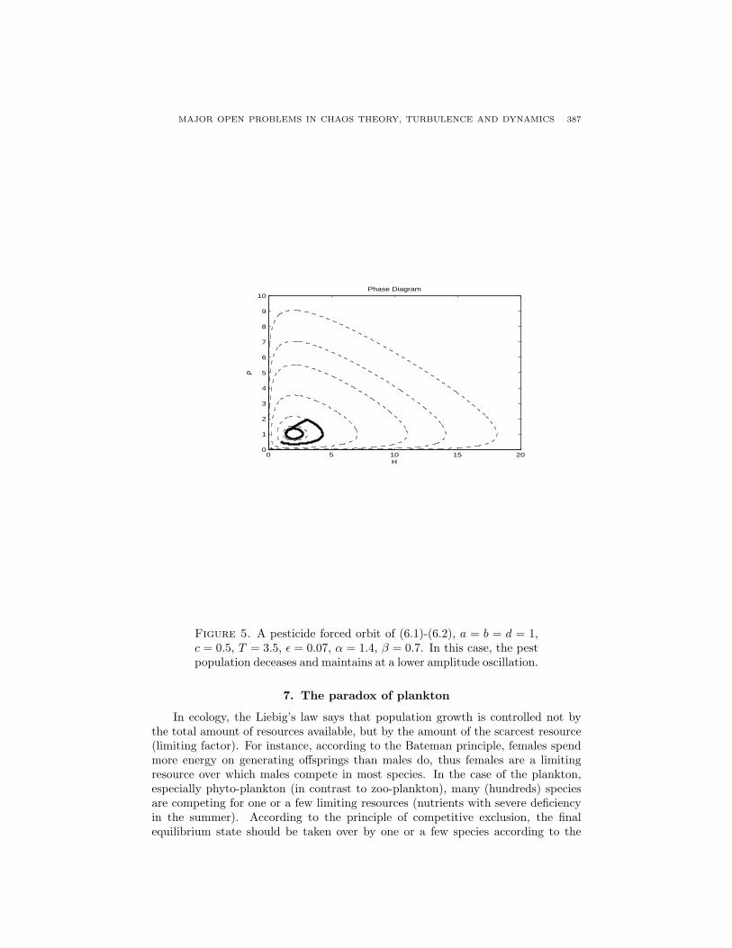
applied when the populations of both the pests and the predators arerelatively large, then a decrease in both populations can be achieved,see Figure 5. On the other hand, if the pesticides are applied when ei-ther the pest’s population or the predator’s population is relatively small,then a dramatic increase in the resurgent pest’s population occurs, lead-ing to pest’s population well beyond the crop’s economic threshold, seeFigures 6 and 7. From these figures, it is clear that even though the pes-ticides only kill the pests rather than their predators (that is, right afterthe application of the pesticides, the pest’s population decreases, whilethe predator’s population maintains the same), the pests still resurge inabundance beyond the crop’s economic threshold. This is because thatwhen the population of the pests decreases, the predator’s population willdecreases too, since the predators feed on the pests. It is the relativelyminimal values of both the pest’s population and the predator’s popula-tion that decide how large the cycle which they are going to sit on in thephase plane.

(2) The amount of pesticides applied is also important. In the case of Figure5, if the amount of pesticides is large enough, a dramatic increase in theresurgent pest’s population can still occur as shown in Figure 8.

The above conclusions also applies when spatial dependence is taken into account[19].

MAJOR OPEN PROBLEMS IN CHAOS THEORY, TURBULENCE AND DYNAMICS 387

0 5 10 15 200

1

2

3

4

5

6

7

8

9

10

H

P

Phase Diagram

Figure 5. A pesticide forced orbit of (6.1)-(6.2), a = b = d = 1,c = 0.5, T = 3.5, ε = 0.07, α = 1.4, β = 0.7. In this case, the pestpopulation deceases and maintains at a lower amplitude oscillation.

7. The paradox of plankton

In ecology, the Liebig’s law says that population growth is controlled not bythe total amount of resources available, but by the amount of the scarcest resource(limiting factor). For instance, according to the Bateman principle, females spendmore energy on generating offsprings than males do, thus females are a limitingresource over which males compete in most species. In the case of the plankton,especially phyto-plankton (in contrast to zoo-plankton), many (hundreds) speciesare competing for one or a few limiting resources (nutrients with severe deficiencyin the summer). According to the principle of competitive exclusion, the finalequilibrium state should be taken over by one or a few species according to the

388 Y. CHARLES LI

0 5 10 15 200

1

2

3

4

5

6

7

8

9

10

H

P

Phase Diagram

Figure 6. A pesticide forced orbit of (6.1)-(6.2), a = b = d = 1,c = 0.5, T = 2, ε = 0.047, α = 0.94, β = 0.47. In this case, thepest population resurges with dramatic increase beyond the crop’seconomic threshold.

limiting factors. On the other hand, in reality hundreds species of the planktoncoexist. This paradoxical question was first raised by Hutchinson [7]. Hutchinsonproposed the idea that this is due to the fact that equilibrium state cannot bereached in reality. Since Hutchinson’s work, there have been many studies on theparadox [28]. The problem involves two branches of chaotic dynamics: fluids andecology.

Plankton drifting in (turbulent) water is an interesting problem for chaoticianto model. Let v(t, x) be the three-dimensional (turbulent) water velocity, wn(t, x)(n = 1, 2, · · · , N) be the plankton drifting velocities relative to water, x ∈ R3. In

MAJOR OPEN PROBLEMS IN CHAOS THEORY, TURBULENCE AND DYNAMICS 389

0 5 10 15 200

1

2

3

4

5

6

7

8

9

10

H

P

Phase Diagram

Figure 7. A pesticide forced orbit of (6.1)-(6.2), a = b = d = 1,c = 0.5, T = 5, ε = 0.039, α = 0.78, β = 0.39. In this case, thepest population resurges with dramatic increase beyond the crop’seconomic threshold.

reality v(t, x) is governed by the Navier-Stokes equations. Numerical simulationsof the full Navier-Stokes equations are still very challenging. We can convenientlymodel the water velocity by a chaotic time evolution of spatial patterns (with vortexstructure). We believe that the essential mechanism of the plankton drifting canbe captured by such a modeling. Let f(t, x) be the density of the limiting resource(deficient neutrient), and ρn(t, x) be the densities of different species of plankton,n = 1, 2, · · · , N . The model is given by

∂tf + (v · ∇)f = −G(ρ1, ρ2, · · · , ρN )f + F (t, x),(7.1)∂tρn + [(v + wn) · ∇]ρn = Hn(f)ρn, n = 1, 2, · · · , N,(7.2)

390 Y. CHARLES LI

0 5 10 15 200

1

2

3

4

5

6

7

8

9

10

H

P

Phase Diagram

Figure 8. A pesticide forced orbit of (6.1)-(6.2), a = b = d = 1,c = 0.5, T = 3.5, ε = 0.149, α = 2.98, β = 1.49. In contrast toFigure 5, here large amount of pesticides is applied, and results inthat the pest population resurges with dramatic increase beyondthe crop’s economic threshold.

whereG(0, 0, · · · , 0) = 0,

and G(ρ1, ρ2, · · · , ρN ) is strictly monotonically increasing in each ρn;

Hn(fn) = 0, where fn are values of f,

Hn(f) is strictly monotonically increasing in f ;

wn = κn∇f + random noise or random walk,

and κn are the drifting coefficients of different plankton.

MAJOR OPEN PROBLEMS IN CHAOS THEORY, TURBULENCE AND DYNAMICS 391

Through G(ρ1, ρ2, · · · , ρN ), different food consumption rates by different speciesof plankton can be introduced. F (t, x) > 0 represents food regeneration, F (t, x)is periodic in t with relatively long period. fn are the ‘critical’ densities of foodfor different species of plankton. Hn(f) model the growth rates from nutrition ofdifferent species of plankton.

References

[1] K. Alligood, T. Sauer, J. Yorke, Chaos, Springer, 1997.[2] R. Devaney, An Introduction to Chaotic Dynamical Systems, 2nd ed., Westview Press, 2003.[3] Z. Feng, Y. Li, A resolution of the paradox of enrichment, submitted (2013). arXiv: 1104.4355.[4] H. Hamilton, The pesticide paradox, Rice Today 1 (2008), 32-33.[5] K. Heong, A. Manza, J. Catindig, S. Villareal, T. Jacobsen, Changes in pesticide use and

arthropod biodiversity in the IRRI research farm, Outlooks on Pest Management October(2007), 1-5.

[6] J. Hinze, Turbulence, McGraw-Hill Press, 1975.[7] G. Hutchinson, The paradox of the plankton, The American Naturalist XCV, No.882

(1961), 137-145.[8] H. Inci, On the well-posedness of the incompressible Euler equation, Dissertation, Univer-

sity of Zurich (2013). arXiv: 1301.5997[9] T. Kreilos, B. Eckhardt, Periodic orbits near onset of chaos in plane Couette flow, Chaos 22

(2012), 047505.[10] A. Labovsky, Y. Li, A Markov chain approximation of a segment description of chaos, Dy-

namics of PDE 7, no.1 (2010), 65-76.[11] Y. Lan, Y. Li, A resolution of the Sommerfeld paradox: numerical implementation, Intl. J.

Non-Linear Mech. 51 (2013), 1-9.[12] P. Lester, H. Thistlewood, R. Harmsen, The effects of refuge size and number on acarine

predator-prey dynamics in a pesticide-distributed apple orchard, J. Applied Ecology 35(1998), 323-331.

[13] Y. Li, Smale horseshoes and symbolic dynamics in perturbed nonlinear Schrodinger equations,J. Nonlinear Sci. 9 (1999), 363-415.

[14] Y. Li, Chaos and shadowing lemma for autonomous systems of infinite dimensions, J. Dy-namics Diff. Eq. 15, no.4 (2003), 699-730.

[15] Y. Li, Segment description of turbulence, Dynamics of PDE 4, no.3 (2007), 283-291.[16] Y. Li, The distinction of turbulence from chaos — rough dependence on initial data, Submitted

(2013). arXiv: 1306.0470[17] Y. Li, Z. Lin, A resolution of the Sommerfeld paradox, SIAM J. Math. Anal. 43, no.4 (2011),

1923-1954.[18] Y. Li, H. Yang, On the arrow of time, submitted (2012). arXiv: 1012.3764.[19] Y. Li, Y. Yang, On the paradox of pesticides, submitted (2012). arXiv: 1303.2681[20] E. Lorenz, Deterministic nonperiodic flow, J. Atmos. Sci. 20 (1963), 130-141.[21] R. May, Simple mathematical models with very complicated dynamics, Nature 261 (1976),

459-467.[22] R. May, Unanswered questions in ecology, Phil. Trans. R. Soc. Lond. B 354 (1999), 1951-

1959.[23] M. Nagata, Three-dimensional finite-amplitude solutions in plane Couette flow: bifurcation

from infinity, J. Fluid Mech. 217 (1990), 519-527.[24] K. Palmer, Exponential dichotomies, the shadowing lemma, and transversal homoclinic

points, Dynamics Reported 1 (1988), 265-306.[25] H. Poincare, Les Methodes Nouvelles de la Mecanique Celeste, vol.I, II, III, 1892. English

translation: New Methods of Celestial Mechanics, ed. by D. Goroff, AIP Press, 1992.[26] O. Reynolds, On the dynamical theory of incompressible viscous fluids and the determination

of the criterion, Phil. Trans. Roy. Soc. Lond. A 186 (1895), 123-164.[27] M. Rosenzweig, Paradox of enrichment: destabilization of exploitation ecosystem in ecological

time, Science 171 (1971), 385-387.[28] S. Roy, J. Chattopadhyay, Towards a resolution of ‘the paradox of the plankton’: A brief

overview of the proposed mechanisms, Ecological Complexity 4 (2007), 26-33.

392 Y. CHARLES LI

[29] S. Smale, Differentiable dynamical systems, Bull. AMS 73, no.6 (1967), 747-817.[30] L. van Veen, G. Kawahara, Homoclinic tangle on the edge of shear turbulence, Phys. Rev.

Lett. 107 (2011), 114501.[31] D. Viswanath, Recurrent motions with plane Couette turbulence, J. Fluid Mech. 580 (2007),

339-358.

Department of Mathematics, University of Missouri, Columbia, MO 65211, USAE-mail address: liyan@missouri.edu

URL: http://www.math.missouri.edu/~cli