Mainmain
123
Lattice Boltzmann simulations of fluid flow in the vicinity of rough and hydrophobic boundaries Von der Fakult¨ at Mathematik und Physik der Universit¨ at Stuttgart zur Erlangung der W¨ urde eines Doktors der Naturwissenschaften (Dr. rer. nat. ) genehmigte Abhandlung vorgelegt von Christian Kunert aus Stuttgart Hauptberichter: P.D. Dr. Jens Harting Mitberichter: Prof. Dr. Udo Seifert Tag der m¨ undlichen Pr¨ ufung: 17.02.2010 Institut f¨ ur Computerphysik der Universit¨ at Stuttgart 2010 1
Transcript of Mainmain

Lattice Boltzmann simulations of
fluid flow in the vicinity of rough
and hydrophobic boundaries
Von der Fakultat Mathematik und Physik der Universitat Stuttgart zur Erlangungder Wurde eines Doktors der Naturwissenschaften (Dr. rer. nat. ) genehmigte
Abhandlung
vorgelegt vonChristian Kunert
aus Stuttgart
Hauptberichter: P.D. Dr. Jens HartingMitberichter: Prof. Dr. Udo Seifert
Tag der mundlichen Prufung: 17.02.2010
Institut fur Computerphysik der Universitat Stuttgart
2010
1

2

Disclaimer
Most results presented in this thesis have been published already in the followingarticles:
• J. Hyvaluoma, C. Kunert, and J. Harting ”Simulations of slip flow on nanobubble-laden surfaces ” Journal of Physics: Condensed Matter 22, in press (2010)
• C. Kunert, J. Harting, and O. I. Vinogradova, ”Random-roughness hydrody-namic boundary conditions ”, Physical Review Letters 105, 016001 (2010).
• J. Harting, C. Kunert, and J. Hyvaluoma, ”Lattice Boltzmann simulations inmicrofluidics: probing the no-slip boundary condition in hydrophobic, rough,and surface nanobubble laden microchannels”, Microfluidics and Nanofluidics8, 1-10 (2010).
• C. Kunert and J. Harting, ”Calibration of lubrication force measurements bylattice Boltzmann simulations”, Proceedings of the 2nd Micro and Nano FlowsConference (2009), ISBN 978-1-902316-72-7 (2009).
• C. Kunert and J. Harting, ”Simulation of fluid flow in hydrophobic roughmicrochannels”, International Journal of Computational Fluid Dynamics 22,475-480 (2008).
• J. Harting and C. Kunert, ”Boundary effects in microfluidic setups”, in NICseries 39: NIC Symposium 2008, edited by G. Munster, D. Wolf, M. Kremer(2008).
• C. Kunert and J. Harting, ”On the effect of surfactant adsorption and vis-cosity change on apparent slip in hydrophobic microchannels”, Progress inComputational Fluid Dynamics 8, 197 (2008).
• C. Kunert and J. Harting ”Roughness induced boundary slip in microchannelflows”, Physical Review Letters 99, 176001 (2007).
3
4
Hiermit versichere ich, dass ich diese Arbeit selbststandig verfasst habe und nurdie angegebenen Quellen und Hilfsmittel benutzt habe.
Christian Kunert, Stuttgart, den 23.09.2010
Contents
1 Zusammenfassung in deutscher Sprache 71.1 Fachlicher Hintergrund und Motivation . . . . . . . . . . . . . . . . . 71.2 Simulationsmethode . . . . . . . . . . . . . . . . . . . . . . . . . . . 81.3 Fluss uber raue Oberflachen . . . . . . . . . . . . . . . . . . . . . . . 91.4 Kraftmessung einer Kugel in der Umgebung einer glatten Oberflache 101.5 Kraftmessung einer Kugel in der Umgebung einer rauen Oberflache . 101.6 Superhydrophobe Oberflachen . . . . . . . . . . . . . . . . . . . . . . 11
2 Introduction 13
3 Slip in microfluidic devices 173.1 How slip is detected . . . . . . . . . . . . . . . . . . . . . . . . . . . . 17
3.1.1 Double focus cross correlation . . . . . . . . . . . . . . . . . . 183.1.2 Micro particle image velocimetry . . . . . . . . . . . . . . . . 193.1.3 Flow rates . . . . . . . . . . . . . . . . . . . . . . . . . . . . . 203.1.4 Force measurement . . . . . . . . . . . . . . . . . . . . . . . . 20
3.2 Reasons for boundary slip . . . . . . . . . . . . . . . . . . . . . . . . 233.3 Surface roughness . . . . . . . . . . . . . . . . . . . . . . . . . . . . . 263.4 Super-hydrophobic surfaces . . . . . . . . . . . . . . . . . . . . . . . 27
3.4.1 Hydrophobic surfaces . . . . . . . . . . . . . . . . . . . . . . . 273.4.2 Rough and hydrophobic surfaces . . . . . . . . . . . . . . . . . 283.4.3 Slip on super-hydrophobic surfaces . . . . . . . . . . . . . . . 29
4 Simulation method 334.1 Molecular dynamics simulations and mesoscopic methods . . . . . . . 33
4.1.1 Molecular dynamics simulations . . . . . . . . . . . . . . . . . 334.1.2 Dissipative particle dynamics . . . . . . . . . . . . . . . . . . 354.1.3 Stochastic rotation dynamics . . . . . . . . . . . . . . . . . . . 36
4.2 The lattice Boltzmann method . . . . . . . . . . . . . . . . . . . . . . 364.2.1 The Boltzmann equation . . . . . . . . . . . . . . . . . . . . . 374.2.2 Concept of lattice Boltzmann . . . . . . . . . . . . . . . . . . 384.2.3 Multi relaxation time approach and macroscopic values . . . . 394.2.4 From lattice Boltzmann to Navier-Stokes . . . . . . . . . . . . 424.2.5 External forces . . . . . . . . . . . . . . . . . . . . . . . . . . 464.2.6 Multi-phase models in lattice Boltzmann . . . . . . . . . . . . 474.2.7 Solid-fluid boundary conditions . . . . . . . . . . . . . . . . . 49
5
6 Contents
4.2.8 Poiseuille flow . . . . . . . . . . . . . . . . . . . . . . . . . . . 54
5 Poiseuille flow over rough surfaces 575.1 The setup . . . . . . . . . . . . . . . . . . . . . . . . . . . . . . . . . 58
5.1.1 Description of roughness . . . . . . . . . . . . . . . . . . . . . 595.1.2 Validation of the simulation method . . . . . . . . . . . . . . 59
5.2 Results . . . . . . . . . . . . . . . . . . . . . . . . . . . . . . . . . . . 625.2.1 Model roughness . . . . . . . . . . . . . . . . . . . . . . . . . 625.2.2 Flow over a realistic surface . . . . . . . . . . . . . . . . . . . 645.2.3 Influence of roughness on the slip length . . . . . . . . . . . . 66
5.3 Rough hydrophobic surfaces . . . . . . . . . . . . . . . . . . . . . . . 67
6 Lubrication force on a sphere approaching a flat surface 716.1 Discretization effects without boundaries . . . . . . . . . . . . . . . . 716.2 The Brenner-Maude theory . . . . . . . . . . . . . . . . . . . . . . . 726.3 Finite size effects with boundaries . . . . . . . . . . . . . . . . . . . . 74
6.3.1 Large test . . . . . . . . . . . . . . . . . . . . . . . . . . . . . 746.3.2 Influence of the system size . . . . . . . . . . . . . . . . . . . 766.3.3 Influence of the radius . . . . . . . . . . . . . . . . . . . . . . 78
6.4 Slip at hydrophobic boundaries . . . . . . . . . . . . . . . . . . . . . 806.4.1 Setup . . . . . . . . . . . . . . . . . . . . . . . . . . . . . . . 806.4.2 Results . . . . . . . . . . . . . . . . . . . . . . . . . . . . . . . 80
7 Lubrication force on a sphere approaching a rough surface 837.1 Setup . . . . . . . . . . . . . . . . . . . . . . . . . . . . . . . . . . . . 837.2 Results . . . . . . . . . . . . . . . . . . . . . . . . . . . . . . . . . . . 867.3 Comparison of roughness and slip . . . . . . . . . . . . . . . . . . . . 867.4 Influence of different parameters . . . . . . . . . . . . . . . . . . . . . 87
7.4.1 Resolution . . . . . . . . . . . . . . . . . . . . . . . . . . . . . 877.4.2 Radius of the sphere . . . . . . . . . . . . . . . . . . . . . . . 897.4.3 Roughness density . . . . . . . . . . . . . . . . . . . . . . . . 907.4.4 Point of contact . . . . . . . . . . . . . . . . . . . . . . . . . . 917.4.5 Heights . . . . . . . . . . . . . . . . . . . . . . . . . . . . . . 93
8 Super-hydrophobic surfaces 958.1 Creation of a super-hydrophobic surface in the lattice Boltzmann
method . . . . . . . . . . . . . . . . . . . . . . . . . . . . . . . . . . 958.2 Results . . . . . . . . . . . . . . . . . . . . . . . . . . . . . . . . . . . 99
8.2.1 Flow profiles . . . . . . . . . . . . . . . . . . . . . . . . . . . . 998.2.2 Slip near super-hydrophobic surfaces . . . . . . . . . . . . . . 101
9 Conclusion 107
Chapter 1
Zusammenfassung in deutscherSprache
1.1 Fachlicher Hintergrund und Motivation
In den letzten Jahren hat die Mikro- und Nanofluidik eine stark wachsende Bedeu-tung in der Industrie gewonnen. Das wurde durch mehrere an Forderprogrammenunterstutzt. Dabei galt die Aufmerksamkeit vor allem dem Design von Mikrokanalen.Die physikalischen Grundlagen des Flusses in kleinen Geometrien wurden aber ver-nachlassigt, obwohl der Fluß in solchen Geometrien meist nicht durch klassischeKontinuumsmethoden beschrieben werden kann. Besonders die Wechselwirkung zwi-schen der Flussigkeit und der Kanalwand spielt in Mikrofluid-Systemen eine wich-tigere Rolle, da das Verhaltnis der Oberflache zum Volumen weit großer ist als inmakroskopischen Systemen. Das bedeutet, dass die Randbedingungen in solchen Sy-stemen besonders genau untersucht werden mussen. In den letzten Jahren ist dabeieine Verletzung der Haftbedingung beobachtet worden. Das hat zur Folge, dass alsRandbedingung in Mikrofluid-Systemen Naviers’ Schlupfbedingung
uy(x0) = β∂uy(x)
∂x|x=0, (1.1)
angewendet werden muss. Dabei ist uy die Flussgeschwindigkeit in y Richtung.
β ist die sogenannte Schlupflange (engl. slip-length) und ∂uy(x)∂x
die Scherrate derFlussigkeit an der Oberflache. Eine anschauliche Interpretation der Schlupflangeist, dass sie die Position innerhalb der Wand angibt, in der das extrapolierte Ge-schwindigkeitsprofil verschwindet. In den letzten Jahren wurden zahlreiche Expe-rimente zur Messung der Schlupflange durchgefuhrt, die abr widerspruchliche Er-gebnisse lieferten – sowohl was den absoluten Wert der Schlupflange angeht alsauch die Abhangigkeiten von verschiedenen Parametern. Mittlerweile gibt es abereinen Konsens daruber, dass Schlupflangen in einfachen Flussigkeiten an hydropho-ben Oberflachen unter einem Mikrometer liegen, typischerweise sogar deutlich unter100nm. Andere Daten lassen auf scheinbaren Schlupf schliessen. Wie dieser scheinba-re Schlupf aber zustande kommt und wovon er abhangt, ist weitgehend unbekannt.Mogliche Ursachen fur diesen Effekt sind die Oberflachenrauigkeit oder die Bildungvon Gasblasen auf der Oberflache.
7
8 Chapter 1. Zusammenfassung in deutscher Sprache
Die Untersuchung dieser Phanomene ist sehr schwierig. Eine analytische Be-schreibung von rauen Oberflachen ist nur in wenigen Fallen moglich. Deshalb sindComputersimulationen hilfreich, um einen tieferen Einblick zu erhalten und so dasscheinbare Auftreten von Schlupf in Experimenten zu verstehen. Dabei ist zu klaren,welche Simulationsmethode geeignet ist. Die Ursache von Hydrophobizitat liegt aufder molekularen Skala. Deshalb waren MD-Simulationen ein angemessenes Mittel.Allerdings sind die verfugbaren Langen- und Zeitskalen zu klein. Klassische CFD-Kontinuums-Loser konnen problemlos diese Langen- und Zeitskalen erreichen, sindaber nicht in der Lage, Wechselwirkungen auf molekularer Skala zu modellieren. Ausdiesem Grund bieten sich sogenannte mesoskopische Methoden an, bei denen nichtdie gesamte Molekulbewegung simuliert wird, sondern nur deren statistisches Mittel.In dieser Arbeit geht es um die Simulation von Fluss in der Umgebung von rauenund hydrophoben Oberflachen mittels der Gitter Boltzmann Methode.
Zu Beginn der Arbeit wird in Kapitel 3 ein Uberblick uber die gangigen Ex-perimente zur Schlupfbestimmung gegeben. Besonderes Augenmerk wird dabei aufExperimente gelegt, die die hydrodynamische Kraft auf eine Kugel an der Spitze ei-nes Kraftfeld-Mikroskops messen, die in einer Flussigkeit gegen die zu untersuchendeOberflache bewegt wird. Die gemessene Kraft F wird dann mit dem theoretischenWert
Fz = −6πR2eµv
hf ∗ (1.2)
verglichen. Die Korrekturfunktion ist durch
f ∗ =1
4
(
1 + 6h
4β
[(
1 +h
4β
)
ln
(
1 +4β
h
)
− 1
])
. (1.3)
gegeben. Dabei ist µ die Viskositat der Flussigkeit, v die Geschwindigkeit und Rder Radius der Kugel. Der Abstand zwischen Kugel und Oberflache ist h. DieSchlupflange β wird dann durch das Anfitten der Korrekturfunktion an die Messwer-te ermittelt.
1.2 Simulationsmethode
Kapitel 4 gibt einen Uberblick uber verschiedene Simulations-Methoden wie Molekular-Dynamik (MD), dissipative Teilchen-Dynamik (DPD), sowie die stochastische Ro-tationsdynamik (SRD). Im Folgenden wird dann die Gitter-Boltzmann-Methode be-schrieben, mit welcher die Simulationen dieser Arbeit durchgefuhrt werden. Dabeibetrachtet man die Dynamik der Einteilchen-Verteilungsfunktion η. Sie ist ein Maß,fur die Wahrscheinlichkeit ein Teilchen mit Geschwindigkeit c am Ort x anzutreffen.Dabei ist der Phasenraum auf einem Gitter diskretisiert. Somit laßt sich die GitterBoltzmann Gleichung als
η(x + ci, ci, t + δt) − η(x, ci, t) = Ω (1.4)
ausdrucken [129]. Dabei ist x der diskretisierte Ort, ci die diskretisierte Geschwin-digkeit, die so gewahlt ist, dass sie in einem Zeitschritt δt, gerade zum nachsten odernachst-nachsten Nachbarn reicht [129]. Der linke Teil der Gleichung gibt an, wie sich

1.3. Fluss uber raue Oberflachen 9
die virtuellen Teilchen frei bewegen, welche durch die Einteilchenverteilungsfunktionbeschrieben werden. Der Kollisionsoperator Ω steht dann fur Kollisionen, die dafursorgen, dass die Verteilung η zu einem Gleichgewicht ηeq tendiert. Die lokale Masseund der Impuls der Flussigkeit bleiben dabei erhalten.
Durch Erweiterungen der Methode ist es moglich, die hydrophobe Flussigkeits-Wand-Wechselwirkung durch eine Shan Chen Kraft
Fwf (x) = Ψfluid(x)∑
i
cigwfΨwall(x + ci) (1.5)
zu modellieren. Dabei ist Ψfluid eine Funktion der lokalen Flussigkeitsdichte, gwf einglobaler Kopplungssarameter und Ψwall ein Maß fur die Hydrophobizitat der Wandan der angegebenen Position x. Es wurde gezeigt, dass solch ein Modell in der Lageist, einen Wandschlupf zu erzeugen, der von der Starke der Wechselwirkung unddem Druck der Flussigkeit abhangt [48].
Ferner ist die Methode in der Lage, sich bewegende Teilchen in der Flussigkeitzu simulieren. Dazu wird die Teilchenwand auf dem Gitter diskretisiert. Die Gitter-wandpunkte tauschen dann ihren Impuls mit der Flussigkeit aus. Auf diese Weisekann auch die gesamte hydrodynamische Kraft, die auf das Teilchen wirkt, bestimmtwerden.
1.3 Fluss uber raue Oberflachen
In Kapitel 5 wird Poiseuille-Fluss uber raue Oberflachen untersucht. Dabei wird dieUberlegung verfolgt, dass sich eine raue Oberflache durch eine effektive Wand be-schreiben laßt, die sich zwischen den Spitzen und den Vertiefungen der Rauigkeitbefindet. Um die Position der effektiven Wand zu bestimmen wird die effektive Ka-nalbreite bestimmt, indem das theoretische Flussprofil an das gemessene angefittetwird. Aus der effektiven Kanalbreite lasst sich dann die effektive Wandhohe bestim-men, welche den Abstand der effektiven Wand zum tiefsten Punkt der Rauigkeitangibt [74].
Es wird zuerst gezeigt, dass die Methode in der Lage ist, die theoretischen Wertefur die effektive Wandposition von Panzer et al. fur sinusformige Rauigkeit wie-derzugeben [108]. Auch konnen die Werte von Lecoq et al. fur eine dreiecksformi-ge Rauigkeit bestatigt werden [88]. Allerdings ist es mittels analytischer Verfahrennicht moglich, komplexere Oberflachen mit starken Variationen zu beschreiben. Ausdiesem Grund ist man zur Untersuchung solcher Oberflachen auf numerische Ver-fahren angewiesen. Da das Verfahren fur die analytisch losbaren Falle die korrektePosition ergibt, werden weitere Modellrauigkeiten untersucht. Das sind Rillen mitquadratischem und dreieckigem, Querschnitt, sowie eine Rauigkeit mit zufalligerRauigkeitshohe an jedem Punkt der Oberflache. Abschließend wird der Fluss ubereine Oberflache simuliert, wie sie in Experimenten verwendet wurde.
Die Ergebnisse lassen sich folgendermassen zusammenfassen: Die Position der ef-fektiven Wand steigt linear mit der maximalen Hohe der Rauigkeit. Sie hangt nur imgeringen Maß von der tatsachlichen Form der Rauigkeit ab. Fur Rillen mit quadra-tischem Querschnitt befindet sich die effektive Wand bei 95% der maximalen Rau-igkeit. Fur Rillen mit dreieckigem Profil bei 85 % und bei gleichverteilten, zufalligen
10 Chapter 1. Zusammenfassung in deutscher Sprache
Rauigkeitselementen bei 92%. Fur die Rauigkeit einer experimentellen Oberflachewurde ermittelt, dass die Position der effektiven Wand an derselben Stelle liegt, wiedie einer zufalligen Oberflache mit derselben gaußformigen Hohenverteilung. Wei-ter wird in diesem apitel festgestellt, dass eine falsch angenommene Wandpositiongroßen Einfluss auf die Schlupfmessung haben kann. Abschließend wird auch ge-zeigt, dass Rauigkeit den Schlupf an hydrophoben Oberflachen sowohl erhohen alsauch herabsetzen kann: je nach Starke der Hydrophobizitat und Hohe der Rauig-keit [74, 76, 49].
1.4 Kraftmessung einer Kugel in der Umgebung
einer glatten Oberflache
In Kapitel 6 wird uberpruft, ob die theoretischen Werte fur die Kraft auf eine Ku-gel in der Nahe der Wand erreicht werden. Das sind wichtige Vorarbeiten, um si-cherzugehen, dass spatere Ergebnisse nicht das Resultat von Simulationsartefaktensind. Dabei wird die simulierte Kraft mit der Theorie von Maude fur eine Kugel,die sich einer Wand nahert, verglichen [95]. Auf diese Weise kann gezeigt werden,dass der Einfluss der Diskretisierung und des begrenzten Simulationsvolumens unterzwei Prozent liegt wenn das Verhaltnis von Systemgroße zu Radius großer als 16/1ist und der Radius mindestens acht Gitterpunkte misst. Außerdem wird uberpruft,ob der Schlupf, der durch die hydrophoben Wande erzeugt wird, auch durch dieKraftmessung erfasst werden kann. Dabei zeigt sich, dass der Schlupf, der durch dieKraftmessung bestimmt wird, wie erwartet, mit dem einer Poiseuille-Flussmessungubereinstimmt.
1.5 Kraftmessung einer Kugel in der Umgebung
einer rauen Oberflache
In Kapitel 7 geht es um die Untersuchung von rauen Oberflachen mittels der Kraft-messung an einer Kugel, die gegen die Wand bewegt wird. Aufgrund der Erkenntnisseaus den vorangegangenen Kapiteln wird zuerst gezeigt, dass sich Rauigkeit in diesemFall auch durch eine effektive Wand beschreiben lasst und nicht durch eine Schlupf-Korrektur wie in Gleichung 1.3. Mittels Poiseuille-Fluss zwischen festen Wandenist es nicht moglich, die beiden Falle genau zu unterscheiden. Es wird uberpruft,wie weit die Annahme einer effektiven Wand gultig ist. Dabei konnte innerhalb derGrenzen der Simulationsgenauigkeit keine Abhangigkeit der effektiven Wandpositionvom Kugelradius, vom Abstand der Kugeloberflache zur Wand oder dem ,,Auftreff-punkt” gefunden werden. Das heisst unter anderem, dass die effektive Wandpositionunverandert bleibt, selbst wenn die maximale Hohe der Rauigkeit grosser als derKugelradius ist.
Ein besonderes Augenmerk liegt auf der Untersuchung von Oberflachen mit ei-ner Rauigkeit, die aus zufallig verteilten, gleich hohen Rauigkeitselementen besteht.Dabei wird festgestellt, dass schon bei einer Bedeckung von nur 10% der Oberflachedie effektive Wandposition bei 90% der Elementhohe liegt. Weiter kann gezeigt wer-
1.6. Superhydrophobe Oberflachen 11
den, dass die Position der effektiven Wand Position fur isotrope Oberflachen mitder fur Poiseuille-Fluss ubereinstimmt. Bei Oberflachen, die eine Vorzugsrichtungaufweisen, wie zum Beispiel Graben, befindet sich die effektive Wand zwischen denWerten fur Fluss in einer der beiden ausgezeichneten Richtungen [78].
1.6 Superhydrophobe Oberflachen
Kapitel 8 beschreibt die Untersuchung von superhydrophoben Oberflachen. Dazuwerden zuerst zwei superhydrophobe Einheitszellen vorgestellt. Die erste besteht auseinem Graben mit quadratischem Querschnitt, dessen Innenwande stark hydrophobsind. Auf diese Weise entsteht eine Dampfblase im Inneren des Grabens uber den dieaussere Flussigkeit mit stark verminderter Reibung fliessen kann. Die Dampfblasekann uber den Rand des Kanals herausragen (oder unter ihm bleiben) und bildet mitder festen Oberflache, den sogenannten Herrausragungswinkel ϕ (engl. protrusionangle). Die zweite Zelle besteht aus einer zylindrischen Aussparung in der Oberflache,deren Innenwande ebenfalls stark hydrophob sind. Wahrend die erste Einheitszelleeine quasi 2D Struktur hat, besitzt die zweite eine echte 3D Struktur.
Die Schlupfeigenschaften der Oberflache werden in diesem Fall wieder durch dasAnlegen eines Poiseuille-Flusses ermittelt und es werden erste Ergebnisse gezeigt.Zunachst werden die Flussprofile in Flussrichtung und orthogonal zur Flussrichtungermittelt und mit den experimentellen Daten von Tsai et al. verglichen [142]. Dabeiwird in guter Ubereinstimmung mit dem Experiment festgestellt, dass das Flussprofilaufgrund der Schlupf-Keinschlupfstreifen in Flussrichtung stark oszilliert. Die Oszil-lation nimmt stark ab, je weiter das Flussprofil von der Wand entfernt aufgenommenwird. Orthogonal zur Flussrichtung ergibt sich ein schlupfbehaftetes Parabelprofil,welches man fur eine derartige Geometrie erwartet. Weiter wird die Abhangigkeitder Schlupflange von ϕ, mit den theoretischen Voraussagen von Davis und Laugaverglichen. Dabei wird beobachtet, dass die Schlupflange stark von ϕ abhangt undein Maximum bei ϕmax = 31 hat. Weiter wird die Schlupflange fur ϕ grosser alsϕci > 70 negativ. Diese Ergebnisse stimmen mit der Theorie von Davis und Laugauberein, allerdings sind die in der Simulation gefundenen Schlupflangen kleiner alsdie vorausgesagten. Das liegt an der relativ großen Grenzflache zwischen der Dampf-und der Flussigkeitsphase. Andererseits nimmt die Theorie perfekten Schlupf aufder Blasenoberflache an. Des weiteren ist ϕ aufgrund der Dicke der Grenzschichtnicht eindeutig definiert. Abschliessend wird dann ermittelt, dass die Blase bei ho-hen Scherraten deformiert wird, was zu einer Reduktion der Schlupflange fuhrt. EinEffekt, der auch von Hyvaluoma und Harting beobachtet wurde [59].
Ausblick
Die Ergebnisse dieser Arbeit zeigen, dass Rauigkeit und Hydrophobizitat zu un-terschiedlichem Verhalten der Flussigkeit an der Oberflache fuhren. Weiter wirdgezeigt, dass das Zusammenspiel aus Rauigkeit und Hydrophobizitat zu unerwarte-ten Phanomenen fuhrt. Wird hingegen die Rauigkeit nicht in die Auswertung von
12 Chapter 1. Zusammenfassung in deutscher Sprache
Experimenten einbezogen, wie beispielsweise bei der Schlupfmessung mittels einesAFM, fuhrt das zu einer groben Ungenauigkeit der Ergebnisse.
Auf Basis der verwendeten Simulationsmethode lassen sich nun auch weitereFragestellungen beantworten. Beispielsweise kann der Einfluss der Deformation vonDampfblasen an superhydrophoben Oberflachen untersucht werden. Einige Expe-rimente beobachten beispielsweise eine Erhohung des Schlupfes mit der Scherrate.Hier wurde vermutet, dass sich die Blasen dabei von der Oberflache losen. Des Wei-teren ware es interessant zu untersuchen, in wie weit sich die Deformation der Blasenauf die Lubrikationskraft in Kraftmessungsexperimenten auswirkt.
Chapter 2
Introduction
During the last decade, micro- and nano-technology has become an important indus-try. This development has been assisted by a funding policy supporting the designof miniaturized mechanical structures and complex micro-machines through whichfluids move. However, the actual transport of fluids in these confined geometrieshave become an area of interest only during the recent years, even though the fluidflow on increasingly smaller scales cannot always be properly described by conven-tional continuum equations: physical phenomena which, can be neglected on themacro scale, become dominant as the length scale diminishes. On the other hand,systems on scales on which micro effects become sensible cannot yet be treated bymolecular methods, owing to the lack of computational power. Hence, there is adefinite need for novel theories, numerical methods, and measurement techniquesdevised to properly describe the confined fluid flow on length scales in the rangefrom 10 and 1000nm.
Reynolds numbers in microfluidic systems are usually small, i.e., usually below0.1. In addition, due to the small scales of the channels, the surface to volumeratio is high causing surface effects like wettability or surface charges to be moreimportant than in macroscopic systems. Also, the mean free path of a fluid moleculemight be of the same order as the characteristic length scale of the system. For gasflows, this effect can be characterized by the so-called Knudsen number [70]. Whilethe Knudsen number provides a good estimate for when to expect rarefaction effectsin gas flows, for liquids one would naively assume that its velocity close to a surfacealways corresponds to the actual velocity of the surface itself. This assumption iscalled the no-slip boundary condition and can be counted as one of the generallyaccepted fundamental concepts of fluid mechanics. However, this concept was notalways well accepted. Some centuries ago, there were long debates about the velocityof a Newtonian liquid close to a surface and the acceptance of the no-slip boundarycondition was mostly due to the fact that no experimental violations could be found,i.e., a so-called boundary slip could not be detected.
In recent years, it became possible to perform very well controlled experimentsthat have shown a violation of the no-slip boundary condition in sub-micron sizedgeometries. Since then, mostly experimental [86, 30, 139, 16, 20, 5, 27, 149, 139], butalso theoretical works [146, 43], as well as computer simulations [130, 3, 23, 136, 140]have been performed to improve our understanding of boundary slip. The topic is
13
14 Chapter 2. Introduction
of fundamental interest because it has practical consequences in the physical andengineering sciences as well as for medical and industrial applications. Interestingly,also for gas flows, often a slip length much larger than expected from classical theorycan be observed. Extensive reviews of the slip phenomenon have recently beenpublished by Lauga et al. [86], Neto et al. [104], as well as Bocquet and Barrat [12].
The reason for such findings is that the behavior of a fluid close to a solid in-terface is very complex and involves the interplay of many physical and chemicalproperties. These include the wettability of the solid, the shear rate or flow velocity,the bulk pressure, the surface charge, the surface roughness, as well as impurities anddissolved gas. Since all those quantities have to be determined very precisely, it isnot surprising that our understanding of the phenomenon is still very unsatisfactory.
A boundary slip is typically quantified by the so-called slip length β – a conceptthat was already proposed by Navier in 1823 [101]. He introduced a boundarycondition where the fluid velocity at a surface is proportional to the shear rate atthe surface (at y = y0), i.e.,
ux(y0) = β∂ux(y)
∂y. (2.1)
In other words, the slip length β can be defined as the distance from the surfacewhere the relative flow velocity vanishes.
The substantial scientific research invested in the slip phenomenon has lead to amore clear picture which can be summarized as follows: one can argue that manysurprising published results were only due to artefacts or misinterpretation of ex-periments. In general, there seems to be an agreement within the community thatslip lengths larger than a few nanometers can usually be referred to as “apparentslip” and are often caused by experimental artefacts. However, the understandingof those artefacts is limited because it involves a large interplay of different param-eters. Besides this, it is interesting whether such an apparent slip is based on aphysical effect that can be technically used or if it is simply a misinterpretation ofexperimental results.
Therefore, it is of importance to perform computer simulations which have theadvantage that most parameters can be changed independently without modifyinganything else. Thus, the influence of every single modification can be studied inorder to present estimates of expected slip lengths or experimental “errors”.
One of the most important deviations between the reality and the idealizedcase which is used for the analysis of the experimental data, is surface roughness.Typically, it is assumed that surface roughness simply increases friction and thereforedecreases any possible slip. However it is still not clear how surface roughness shouldbe treated in microfluidic setups. This problem becomes more serious when thesurface becomes hydrophobic, since hydrophobicity is known to cause slip [86, 104,12]. Here, the interplay of roughness can cause so-called super-hydrophobicity, as itis known in the lotus effect [115]. In this thesis, computer simulations are appliedto investigate the influence of roughness and the influence of the combination ofroughness and hydrophobicity on the slip phenomenon.
The simulation method used to study microfluidic devices has to be chosen care-fully. While Navier-Stokes solvers are able to cover most problems in fluid dynamics,they lack the possibility to include the influence of molecular interactions as needed
15
to model boundary slip. Molecular dynamics (MD) simulations are the best choiceto simulate the fluid-wall interaction, but the computer power today is not sufficientto simulate length and time scales necessary to achieve orders of magnitude whichare relevant for experiments. However, boundary slip with a slip length β of theorder of many molecular diameters σ has been studied with molecular dynamicssimulations by various authors [136, 23, 24, 5, 111]. The problem of MD simulationsis that the achievable time- and length scales are very small. Therefore, mesoscopicsimulation methods should be applied to describe phenomena in microfluidics.
This work focuses on numerical investigations of the slip phenomenon by meansof lattice Boltzmann simulations with a strong focus on roughness and the interplaybetween roughness and wetting phenomena. To do so, two different slip measurementmethods are simulated. One is to apply a Poiseuille flow between two patternedboundaries, and to record the flow profile. Then, the profile can be compared tothe theoretical one, which assumes a slip boundary condition. The second methodrecords the drag force that is acting on a sphere which is moved with a constantvelocity towards the observed surface. Due to the influence of the boundary, thedrag force acting on the sphere is disturbed and a correction function is needed todescribe the measured force. This correction function, which depends on the slip, isfitted via the slip length towards the recorded force.
The lattice Boltzmann method has to be extended to be able to simulate hy-drophobic boundaries by means of a repulsive fluid-boundary interaction. Further,it is necessary to implement a multi-phase model to simulate liquid- and gas phasesin the vicinity of the boundary. Both tasks can be achieved by a Shan-Chen interac-tion [124, 126]. The next important enhancement is the implementation of movingobjects. Ladd et al. have developed a method to implement this [82]. A detaileddescription of the simulation method which is applied here is given in chapter 4.
In chapter 5, fluid flow in the vicinity of rough surfaces is investigated. Here,different model roughnesses and experimental surfaces are implemented in the sim-ulation. The roughness is described by means of an effective boundary position thatcorresponds to a virtual plane at which the no-slip boundary condition holds. Animportant finding is the fact that the effective boundary position mainly dependson the maximum height of the roughness elements but only to a small extent on theactual shape or the detailed position of them [74].
An alternative way of investigating boundaries is the measurement of the dragforce acting on a sphere that is approaching a surface. Since the boundary conditionon the surface is changing the fluid flow in its vicinity and thus the drag force createdby the flow around the sphere changes. This effect is utilized in many experimentswhere typically a sphere is attached to the cantilever of an atomic force microscopewhich approaches a surface [146, 147, 128, 13, 156, 157]. To simulate such a behaviorit is essential to understand the limits of the applied simulation method. Therefore,detailed studies of finite size and discretization effects in a system of a sphere, whichis approaching a flat surface, are performed in chapter 6 [77]. Further, it is shownthat the results for the slip length β in a Poiseuille flow and a drag force measurementare equivalent. Therefore, it is possible to utilize the simulation scheme to investigateother boundary properties as well.
In chapter 7, the findings of chapter 6 are used to investigate the influence of a
16 Chapter 2. Introduction
rough surface on the drag force. Here, it is possible to demonstrate that the dragforce shows a different asymptotic behavior when the sphere is approaching a roughor a slippery surface. A rough surface can be described by an effective boundaryposition that leads to a shift of the recorded force curve, while a slip surface requiresa complex correction function [78]. This finding is important because it is notpossible to distinguish a shift or slip in a Poiseuille or Couette flow setup with fixedseparation between the boundaries. However, the question of the correct boundarycondition is fundamental in nature.
After the investigation of rough surfaces the interplay of roughness and hydropho-bicity is of interest. Here, the focus lies on the flow over so-called super-hydrophobicsurfaces. At these surfaces, a gas bubble is trapped in the asperities of the surfaceroughness, leading to a decreased friction. In chapter 8, two super-hydrophobic cellsare presented. In addition, Poiseuille flow over such surfaces is studied and thepreliminary findings are compared to analytical and experimental studies. A goodagreement to experimental data is found considering the flow profiles and the de-pendence of the slip length on the protrusion angle, which depicts how strongly thebubble invades into the bulk fluid. Further, a shear dependence of the slip length isdetected due to the deformation of the bubbles trapped in the roughness.
The results show that the roughness has an influence on slip measurements. Incase of a wrongly assumed boundary condition, large apparent slip length could bemeasured. Further, the interplay of roughness and hydrophobicity can lead to both,an increase and a decrease of the apparent slip. Here, future research can be doneapplying the presented methods.
Chapter 3
Slip in microfluidic devices
For more than a century the no-slip boundary condition, stating that the velocityof a fluid close to a solid boundary is equal to the boundary velocity, was assume todescribe fluid flow. Its wide acceptance is founded on the fact that no experimentalviolation was found on a macroscopic length scale. To characterize slip in 1823Navier [101] postulated a slip boundary condition stating that the flow velocity v atthe boundary at x = 0 is proportional to the shear rate and the so-called slip lengthβ,
v(x = 0) = β∂v
∂x|x=0. (3.1)
In the recent years, fluid flow in micro and nano sized geometries has become apopular research topic. Here, several experiments have been performed that showeda violation of the no-slip boundary condition, which can be explained by Navier’sslip boundary condition (or its tensorial generalization [7]). However, typical sliplengths are found to be less than one µm.
In the following chapter an overview on typical slip experiments is given. Further,some controversial findings are presented and different dependencies are discussed.Those contradicting experimental results are the starting point for this thesis. There-fore, it is necessary to understand the fundamentals of the experimental setups andpossible error sources.
3.1 How slip is detected
In recent years, it became possible to perform very well controlled experiments thathave shown a violation of the no-slip boundary condition in sub-micron sized geome-tries. Since then, mostly experimental [86, 30, 139, 16, 20, 5, 27, 149, 139], but alsotheoretical works [146, 43], as well as computer simulations [130, 3, 23, 136, 140] havebeen performed to improve our understanding of boundary slip. However, many re-sults are contradicting each other concerning the value of slip and the influence ofdifferent parameters. Extensive reviews of slip phenomena have been published re-cently by Lauga et al. [86], Neto et al. [104], and Bocquet and Barrat [12]. Therefore,only a short overview on the topic will be given.
In this section the most common experiments, simulations and theories aboutboundary slip are discussed. A strong focus lies on the experiments based on force
17

18 Chapter 3. Slip in microfluidic devices
measurements, since they are the foundation of this thesis. Then an overview onpossible parameters that have an influence on the slip length β is given and reasonsfor the development of slip are discussed.
3.1.1 Double focus cross correlation
LASER
Particles
Detector 1 Detector 2
Computer
Figure 3.1: Cartoon of the cross correlation method. The particles are illuminatedby the foci of two laser beams. By calculating the time cross-correlation functionthe velocity between the two foci can be derived.
For the cross correlation method fluorescent particles are brought into the flow.Typically, a laser beam split into two beams is used to illuminate the particles. Thetwo beams can be focused at a fixed distance at a fixed location. By having twobeams at a fixed distance it is possible to record every particle that crosses one ofthe focal points of the beams. The technique rests in the premise that only a smallnumber of labeled particles are simultaneously located in an effective focal volumeof the order of 10−15l. Therefore the time cross-correlation can be used to determinethe average time a particle needs to cross the second focus after it crosses the firstone. A time cross-correlation function g2(t) may generally be derived from any twotime-resolved intensities I1(t
′), I2(t′). It is calculated via
g2(t) =〈I1(t
′)I2(t′ + t)〉t′
〈I1(t′)〉t′〈I2(t′)〉t′,
with 〈...〉t′ denoting the ensemble average for an ergodic system. The quantity In(t′)is given by the fluorescence intensity detected by focus n at time t′. Typically thetime cross-correlation function exhibits a local maximum tm which is the averagetime a particle needs to travel from one focus to the other.
Since the focus of the laser beams can be located very precisely one has an accu-rate measurement of the flow velocity at a given point [91]. Pit et al. have applied

3.1. How slip is detected 19
the cross correlation method for hexadecan flowing on a hydrocarbon lyophobicsmooth surface, and found a slip length of 400nm [110].Vinogradova et al. refinedthe method and determined a slip length for water and NaCl aqueous solution ofless than 100nm which is independent on the shear rate and the salt-concentration,at a hydrophobic polymer channel. For hydrophilic surfaces no measurable slip wasdetected [148] .
3.1.2 Micro particle image velocimetry
A common tool for the measurement of flows is the so-called particle image velocime-try (PIV). The method is very similar to the cross correlation method, but insteadof just taking into account single events of a particle crossing the focus of a laserbeam, one takes a whole video and correlates the single frames to each other, in asimilar way as described in the section above.
LASER
Particles
MicroscopeCamera
Figure 3.2: A cartoon of the PIV method. The particles are illuminated by a laserand their movement is recorded by a camera through a microscope. The data isthen analysed by a computer by calculating the cross-correlation function betweenconsecutive frames.
The simplest form of micro-PIV is to illuminate the whole micro-channel undera microscope and to take an video. The disadvantage of such a setup is that possibleframe rates are low so the correlation is highly disturbed by the Brownian motion ofthe particles. Therefore typically the volume is illuminated by two laser pulses withdifferent wave length. By this, the autocorrelation can be determined on a muchsmaller timescale, which reduces the noise.
Tretheway and Meinhart [138, 139] applied micro PIV in hydrophobic glass chan-nels and measured slip lengths of up to 1µm. However Joseph and Tabeling [67]found slip lengths of less than 100nm, stating that this is the minimal resolution ofthe method, i.e., that it is doubtful whether there is any slip.
Both methods have systematic problems in the measurement of slip in Newtonianfluids. The basic assumption of the methods is that the particles have the same
20 Chapter 3. Slip in microfluidic devices
velocity as the fluid and that the particles do not disturb the fluid flow. In case ofsimple fluids on a length scale that is not large compared to the particle size thoseassumptions might not be valid. Further, the particles might interact directly withthe boundary which influences their velocities.
3.1.3 Flow rates
A less direct method to measure the slip length is to measure the mass flow Q =∫
ρvdA through a pipe and compare the ratio between the theoretical value QPoiseuille
and the measured one Qβ. Here v is the flow velocity and A is the cross-section ofthe pipe. For a circular pipe with radius R the slip length can be calculated via
Qβ
QPoiseuille
= 1 +4β
R. (3.2)
Experiments of this kind have been performed by different groups using differentfluids and different channels. An early experiment was performed by Schnell in 1956,finding a slip length of β = 1...10µm [122]. However, this early experiments sufferfrom a lack of accuracy. More recent experiments report slip lengths of 10 − 70nm[138]. For an overview on slip measurements several reviews have been publishedrecently [104, 86, 12, 90]. The measurement of the flow rate has several problems.The first one is that it is hard to exactly measure the parameters that enter theflow rate like the radius of the channel or the exact pressure drop. The seconddrawback of the method is that all deviations to the flow rate automatically resultin a measured slip length. Therefore one obtains no deeper understanding of apotential slip mechanism.
3.1.4 Force measurement
A very popular way to measure fluid slip is the measurement of the lubrication forceacting on a sphere that is approached towards a surface. Since such experiments areone of the background of this thesis, a more detailed overview on their theoreticalbackground is given here.
The main theory was developed by O.I. Vinogradova [149, 150, 147, 146] and is anextension of the Reynolds lubrication theory adopted for slip surfaces. For simplicitythe derivation concentrates on spherical rigid bodies instead of arbitrarily curvedsurfaces as presented in [69]. Additionally the focus lies on the case where a no-slipboundary condition is applied on one sphere with radius R1 approaching anothersphere with infinite radius R2 (i.e. a flat surface). According to the symmetry acylindrical coordinate system (r, θ, Z) is employed, thus the spheres move along thez-axis. The angular direction θ drops out. The distance between the two surfaces is hand the approaching velocity is v. The two surfaces can be described by paraboloids:
Z = h +1
2
r2
R1
+ O(r4)
and
Z = −1
2
r2
R2
+ O(r4)

3.1. How slip is detected 21
By shifting coordinates with z = Z+r2/(2R2) and Re = R1R2/(R1+R2) the surfacesread as
z = h +1
2
r2
Re
+ O(r4)
andz = O(r4).
From the Stokes equation of a fluid with viscosity µ, pressure gradient ∇p and thefluid velocity of u
µ∇2u = −∇p
we get
µ∂2ur
∂z2=
∂p
∂r(3.3)
when assuming that pressure gradient in z-direction vanishes ∂p∂z
= 0. This impliesthat the pressure is a function of r only. On the lower boundary we now assume aslip boundary condition with the slip length β, which reads as
uz = 0
and
ur = β∂ur
∂zwhile on the top surface we apply the no-slip boundary condition so we get
uz −rur
Re
= −v
andur = 0.
In the original paper by O.I. Vinogradova [146] an arbitrary slip β1 is assumed butfor simplicity we focus on the case that is applied in this thesis, i.e. β1 = 0. Thesolution of Eq. 3.3 with the given boundary conditions reads now as
ur =1
2µ
∂p
∂r
[
z2 − zH2
H + β− βH2
H + β
]
,
where H = h + r2
2Re. Further, the continuity equation
∂uz
∂z+
1
r
∂(rur)
∂r= 0
has to be fulfilled. By integrating we get
v =1
r
∂
∂r
[(
r∂p
∂r
)
∂p
2µ
(
H3
33 − H4
2(H + β)− βH3
H + β
)]
which gives us the dependence of the flow field on the constant relative velocity v ofthe spheres. Due to this we have obtained a differential equation of the pressure p:
d
dr
(
X−1rdp
dr
)
= 2µvr (3.4)
22 Chapter 3. Slip in microfluidic devices
where
X =6(β + H)
−H3(H + 4β).
By integrating Eq. 3.4 two times while assuming p = 0 for r → ∞ and due to therotational symmetry dp
dr= 0 at r = 0 one obtains
p = −3µRev
H2p∗,
with the dimensionless correction function
p∗ =1
42
H
3β
[
1 − H
4βln(1 +
4β
H)
]
,
The hydrodynamic resistance force F on the upper sphere is now the inverted of theone acting on the lower surface. Therefore it can be calculated as
Fz = −∫ ∞
0
(
−p + 2µdvz
dz
)
2πr dr.
Since the contribution of the outer region can be neglected one concludes that thepressure term is dominant and one ends up with
Fz = −6πR2eµv
hf ∗ (3.5)
where
f ∗ =1
4
(
1 + 6h
4β
[(
1 +h
4β
)
ln
(
1 +4β
h
)
− 1
])
. (3.6)
In the case of a flat lower surface, as discussed above, Re will become the radius ofthe upper sphere R. The force is valid for small distances h and slow approachingvelocities v. Eq. 3.5 is widely used in experiments, but here some corrections haveto be applied, due to deviations from the ideal case. Such deviations include theacceleration of the sphere due to surface forces, or the drag force of the cantilever.
A typical experimental setup is shown in Fig. 3.3. On the cantilever of an atomicforce microscope (AFM) or a surface force apparatus (SFA) a silicon sphere is at-tached. Then the surface is approached towards the sphere while the distance andthe force are recorded and compared with Eq. 3.5 using the slip length β in f ∗ as afit parameter.
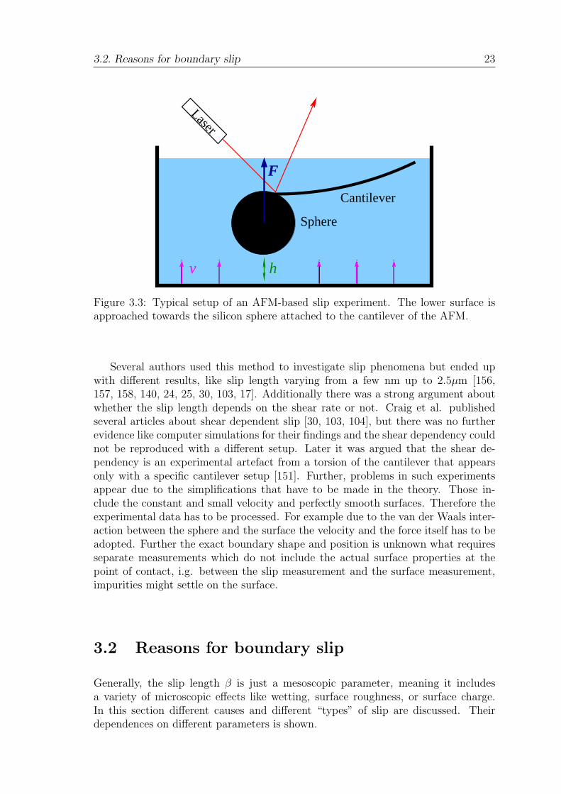
3.2. Reasons for boundary slip 23
Sphere
Cantilever
Laser
F
v h
Figure 3.3: Typical setup of an AFM-based slip experiment. The lower surface isapproached towards the silicon sphere attached to the cantilever of the AFM.
Several authors used this method to investigate slip phenomena but ended upwith different results, like slip length varying from a few nm up to 2.5µm [156,157, 158, 140, 24, 25, 30, 103, 17]. Additionally there was a strong argument aboutwhether the slip length depends on the shear rate or not. Craig et al. publishedseveral articles about shear dependent slip [30, 103, 104], but there was no furtherevidence like computer simulations for their findings and the shear dependency couldnot be reproduced with a different setup. Later it was argued that the shear de-pendency is an experimental artefact from a torsion of the cantilever that appearsonly with a specific cantilever setup [151]. Further, problems in such experimentsappear due to the simplifications that have to be made in the theory. Those in-clude the constant and small velocity and perfectly smooth surfaces. Therefore theexperimental data has to be processed. For example due to the van der Waals inter-action between the sphere and the surface the velocity and the force itself has to beadopted. Further the exact boundary shape and position is unknown what requiresseparate measurements which do not include the actual surface properties at thepoint of contact, i.g. between the slip measurement and the surface measurement,impurities might settle on the surface.
3.2 Reasons for boundary slip
Generally, the slip length β is just a mesoscopic parameter, meaning it includesa variety of microscopic effects like wetting, surface roughness, or surface charge.In this section different causes and different “types” of slip are discussed. Theirdependences on different parameters is shown.
24 Chapter 3. Slip in microfluidic devices
a) b) c)
β
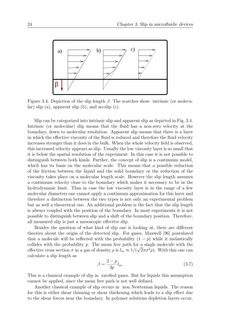
Figure 3.4: Depiction of the slip length β. The scatches show: intrinsic (or molecu-lar) slip (a), apparent slip (b), and no-slip (c).
Slip can be categorized into intrinsic slip and apparent slip as depicted in Fig. 3.4.Intrinsic (or molecular) slip means that the fluid has a non-zero velocity at theboundary, down to molecular resolution. Apparent slip means that there is a layerin which the effective viscosity of the fluid is reduced and therefore the fluid velocityincreases stronger than it does in the bulk. When the whole velocity field is observed,this increased velocity appears as slip. Usually the low viscosity layer is so small thatit is below the spatial resolution of the experiment. In this case it is not possible todistinguish between both kinds. Further, the concept of slip is a continuum model,which has its basis on the molecular scale. This means that a possible reductionof the friction between the liquid and the solid boundary or the reduction of theviscosity takes place on a molecular length scale. However the slip length assumesa continuum velocity close to the boundary which makes it necessary to be in thehydrodynamic limit. Thus in case the low viscosity layer is in the range of a fewmolecular diameters one cannot apply a continuum approximation for this layer andtherefore a distinction between the two types is not only an experimental problembut as well a theoretical one. An additional problem is the fact that the slip lengthis always coupled with the position of the boundary. In most experiments it is notpossible to distinguish between slip and a shift of the boundary position. Therefore,all measured slip is just a mesoscopic effective slip.
Besides the question of what kind of slip one is looking at, there are differenttheories about the origin of the detected slip. For gases, Maxwell [96] postulatedthat a molecule will be reflected with the probability (1 − p) while it inelasticallycollides with the probability p. The mean free path for a single molecule with theeffective cross section σ in a gas of density ρ is lm ≈ 1/(
√2πσ2ρ). With this one can
calculate a slip length as
β =2 − p
3plm. (3.7)
This is a classical example of slip in rarefied gases. But for liquids this assumptioncannot be applied, since the mean free path is not well defined.
Another classical example of slip occurs in non Newtonian liquids. The reasonfor this is either shear thinning or shear thickening which leads to a slip effect dueto the shear forces near the boundary. In polymer solutions depletion layers occur.
3.2. Reasons for boundary slip 25
Here, the polymers are not entering an area close to the boundary[152]. Since thesolution has a higher viscosity than the solvent, apparent slip occurs [49].
The most simple explanation of slip is the low friction between the boundaryand the fluid molecules, compared with the inner friction of the liquid [83]. Reasonsmight be repulsive forces between the fluid and the boundary, like at hydrophobicboundaries. However, this effect is small since other effects like the surface roughnessgenerally increase the friction so it is questionable whether the low molecular frictionovercompensates this unless there is a mechanism that creates more slip due toroughness. The surface-fluid interaction that causes the slip might be increased bythe roughness due to the larger total surface.
One way to decrease the friction is the formation of nano-bubbles. They areeither formed by solved gas or vapor that forms bubbles in pockets created by thesurface roughness. Since the viscosity of the gas inside the bubbles is very low thefluid will slide over this film of bubbles [43, 142]. Specially designed surfaces can beproduced to create gas or vapor bubbles. Such surfaces show a very large contactangle and therefore are called super-hydrophobic surfaces which will be discussedlater. A way to create such surfaces is the deposition of carbon nanotubes to formso-called carbon nanotube forests [25, 66, 26]. Another possible geometry are groovesthat are filled with vapor [142].
In the case that the surface roughness is of the same order of magnitude as thesize of the fluid molecules the molecules get trapped inside the roughness, but inthe case where the molecules are significantly larger, they will just roll over theroughness. In consequence the friction is reduced and slip occurs. This effect isknown for friction of solid state bodies [73] and MD simulations came to similarconclusions [39, 40].
Another phenomenon in a fluid near a solid surface is the ordering of the fluidmolecules according to the crystal structure of the solid boundary. Due to thisordered fluid layers are formed which can slide over each other with reduced fric-tion [132, 120].
Due to the variety of different effects that influence the surface-fluid interactionand therefore the slip length, one observes a significant dispersion of the results foralmost similar systems [86, 104]. For example, observed slip lengths vary between afew nanometers [21] and micrometers [139] and while some authors find a dependenceof the slip on the flow velocity or shear rate [20, 156, 30], others do not [16, 139].
However, the substantial scientific research during the past few years allows todraw a clearer picture that can be summarized as follows: many surprising resultspublished were only due to artifacts or misinterpretation of experiments. In generalthere seems to be an agreement within the scientific community that slip lengths insimple fluids larger than ”a few nanometers” can usually be referred to as apparentslip and are often caused by experimental artefacts. Small slip length are even harderto determine experimentally and require sophisticated methods like the presentedAFM measurements or well controlled micro PIV experiments.
Extensive reviews of the slip phenomenon have recently been published by Laugaet al. [86], Neto et al. [104], as well as Bocquet and Barrat [12]. This brief intro-duction to the topic should give a sufficient overview for this thesis while a deeperinsight is given by the cited literature.
26 Chapter 3. Slip in microfluidic devices
3.3 Surface roughness
One important parameter entering the slip length β is the surface roughness thatcannot be neglected if the height of the roughness is of the same magnitude as typicallength scales of the system. The influence of roughness on β has been investigatedby numerous authors. The first idea is that roughness leads to higher drag forcesand thus to no-slip on macroscopic scales. Richardson showed analytically thatwhen looking on a no-shear (full-slip) surface with a periodic roughness a significantdrag force arises that leads to a finite slip length and in the continuum limit tono-slip [114].
Panzer et al. calculated the slip length β analytically for Poiseuille flow withrough walls by performing a Fourier expansion of the streaming function Ψ con-taining the solution of the Navier-Stokes equations in the laminar case [108]. Ψ isobtained by a Fourier expansion of the boundary surface and of the pressure fieldand its solution contains information of an effective boundary. The problem of suchan approach is that it works only for small wave numbers. One would have to takeinto account an infinite number of terms to achieve a result for arbitrary geometries.Panzer et al. gave an analytical equation for β in the case of small cosine-shapedsurface variations [108]. It is applicable to two infinite planes separated by a distance2d being much larger than the highest peaks rmax. Surface variations are determinedby peaks of height rmax, valleys at rmin = 0 and given by r(z) = rmax
2+ rmax
2cos(qz).
Here, q is the wave number. Since the surfaces are separated by a large distance, thecalculated slip length is equal to the negative effective boundary reff that is foundto be
reff = −β =rmax
2
(
1 + k1 − 1
4k2 + 19
64k4 + O(k6)
1 + k2(1 − 12k2) + O(k6)
)
. (3.8)
The first and k-independent term shows the linear behavior of the effective heightreff on the average roughness Ra = rmax/2. Higher order terms cannot easily becalculated analytically and are neglected. Thus, Eq. 5.2 is valid only for k = qrmax
2≪
1. However, for realistic surfaces, k can become substantially larger than 1 causingthe theoretical approach to fail. This shows that for flow over a rough surface one haseither to assume an effective boundary position inside the boundary or to describethe flow by a slip boundary condition.
Lecoq and coworkers [88] performed experiments with well defined roughness,and developed a theory to predict the position of the effective boundary. For theexperiments they utilised a laser interferometer to measure the trajectory of a col-loidal sphere and thereby determined the lubrication force and an effective boundaryposition. The used geometry consists of grooves with a triangular profile. For a the-oretical description the boundary is expressed in a Fourier series that gives theboundary condition for the Laplace equation. From this an effective boundary canbe derived by a fast converging series. The approach is very similar to the theoryof Panzer et al. and only varies in details and in the investigated surface, i.e., theshape being triangular instead of sinusoidal.
However, an analytical description of the flow near an arbitrarily rough surfaceis not possible [83]. The reason is that the surface has to be expressed in an expan-sion that enters the covering flow equations but the higher orders of the expansion
3.4. Super-hydrophobic surfaces 27
cannot be neglected in an arbitrary geometry. Thus, the correct boundary conditionis unknown. Therefore in classical boundary layer theory the usage of the ”sandequivalent” is still in use [119]. This means that a rough surface is compared to asurface with sand of different grain sizes glued on it.
Besides the obvious creation of friction there are some cases were roughness leadsto a slip effect. Jansons has shown analytically that even few perturbations on flatsurfaces lead to mesoscopic slip [64]. This was experimentally demonstrated byMcHale and Newton [98]. Jabbarzadeh et al. performed molecular dynamics (MD)simulations of Couette flow between sinusoidal walls and found that slip appears forroughness amplitudes smaller than the molecular length scale [63]. Also, it can causepockets formed by the corrugations of the surface, to be filled with vapor or gas nano-bubbles leading to apparent slip [33, 66]. Molecular dynamics simulations (MD)have been applied to investigate roughness as well [154, 1]. Recently, Sbragagliaet al. applied the LB method to simulate fluids in the vicinity of microstructuredhydrophobic surfaces [117] and Varnik et al. showed that even in small geometriesrough channel surfaces can cause flow to become turbulent [144].
3.4 Super-hydrophobic surfaces
In recent years specially designed surfaces have become popular. In the contextof fluid dynamics and with a special focus on slip phenomena so-called super-hydrophobic surfaces are of great interest. A review of the topic was written byRothstein [115].
3.4.1 Hydrophobic surfaces
When talking about wettability, one typically assumes a liquid drop on a solid sur-face surrounded by vapor. The wettability of a surface is defined by the spreadingcoefficient S = γSV − γLV − γLS where γSV , γLV , and γLS are the solid-vapor, liquid-vapour, and liquid-solid interfacial tensions. For spreading coefficients greater thanzero S > 0, the solid is fully wetted by the liquid whereas for S < 0, the solid is onlypartly wetted by the liquid, which forms a spherical end cap with an equilibriumcontact angle θ defined by Young’s law as [155]
θ = cos−1 γSV − γLS
γLV
.
For surfaces with contact angle θ < 90 the surface is considered hydrophilic, whereasθ > 90 is called hydrophobic as depicted in Fig. 3.5. However, this applies onlyto the equilibrium contact angle. Due to surface roughness and other effects likechemical heterogenity a variety of contact angles is possible, depending on the actualwetted parts of the surface on the micro scale or in other words it depends on the“history” of the wetting process. This non-uniqueness of the contact angle is knownas contact angle hysteresis [41].

28 Chapter 3. Slip in microfluidic devices
θ
a) b)
θ
Figure 3.5: A liquid drop on a surface forms a contact angle θ with the surface.For θ > 90 the surface is considered as hydrophobic (a), whereas θ < 90 is calledhydrophilic (b).
The influence of the wettability on the slip was investigated by various authors.Results showed, that hydrophobicity can cause slip lengths much larger than themean free path. Thompson and Trojan [137] performed molecular dynamics (MD)simulations and found a nonlinear increase of the slip velocity at large (unphysical)shear rates and that the slip length diverges at a critical shear rate. Barrat andBocquet [3, 10, 11] showed that the slip length can be larger than 40 moleculardiameters in the linear (shear independent) regime that corresponds to experimentalshear rates. The slip results from a liquid depletion layer near the wall. Within thislayer, the density and thus the viscosity are decreased resulting in a large apparentslip. However, the possible slip length that can be achieved by plane hydrophobicsurfaces is limited to some tens of nanometers and for a stronger effect some surfacestructure is needed.
3.4.2 Rough and hydrophobic surfaces
Super-hydrophobic surfaces were originally inspired by the strong water repellentproperties of the Lotus leaf [4]. Barthlott and Neinhuis stated that a very largecontact angle and a small contact angle hysteresis is responsible for the efficientself cleaning behavior of the plant’s leaf and called this behavior super-hydrophobic.Due to the small hysteresis a drop becomes unstable to small perturbations on thesurface and starts to roll over it.
Synthetic super-hydrophobic surfaces have been created recently by a variety ofgroups. They achieve a contact angle of nearly 180 with little to no measurable con-tact angle hysteresis. The difference between a hydrophobic and a super-hydrophobicsurface lies not in the surface chemistry but in the surface structure or its topology.As an example the Lotus leaf has micrometer sized protrusions that are covered withhydrophobic wax.
One distinguishes between two different states that characterize a hydrophobicrough surface. The first one is the Wenzel state [153] in which all surface asperities
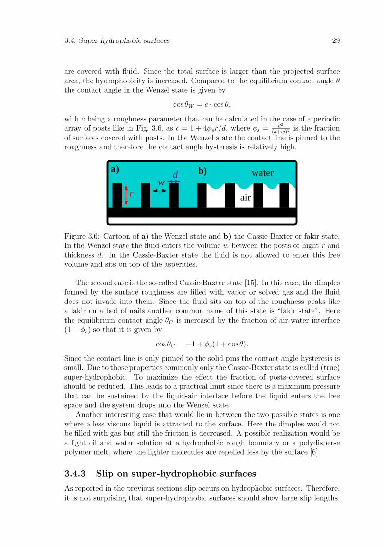
3.4. Super-hydrophobic surfaces 29
are covered with fluid. Since the total surface is larger than the projected surfacearea, the hydrophobicity is increased. Compared to the equilibrium contact angle θthe contact angle in the Wenzel state is given by
cos θW = c · cos θ,
with c being a roughness parameter that can be calculated in the case of a periodicarray of posts like in Fig. 3.6, as c = 1 + 4φsr/d, where φs = d2
(d+w)2is the fraction
of surfaces covered with posts. In the Wenzel state the contact line is pinned to theroughness and therefore the contact angle hysteresis is relatively high.
r
dw
water
air
b)a)
Figure 3.6: Cartoon of a) the Wenzel state and b) the Cassie-Baxter or fakir state.In the Wenzel state the fluid enters the volume w between the posts of hight r andthickness d. In the Cassie-Baxter state the fluid is not allowed to enter this freevolume and sits on top of the asperities.
The second case is the so-called Cassie-Baxter state [15]. In this case, the dimplesformed by the surface roughness are filled with vapor or solved gas and the fluiddoes not invade into them. Since the fluid sits on top of the roughness peaks likea fakir on a bed of nails another common name of this state is “fakir state”. Herethe equilibrium contact angle θC is increased by the fraction of air-water interface(1 − φs) so that it is given by
cos θC = −1 + φs(1 + cos θ).
Since the contact line is only pinned to the solid pins the contact angle hysteresis issmall. Due to those properties commonly only the Cassie-Baxter state is called (true)super-hydrophobic. To maximize the effect the fraction of posts-covered surfaceshould be reduced. This leads to a practical limit since there is a maximum pressurethat can be sustained by the liquid-air interface before the liquid enters the freespace and the system drops into the Wenzel state.
Another interesting case that would lie in between the two possible states is onewhere a less viscous liquid is attracted to the surface. Here the dimples would notbe filled with gas but still the friction is decreased. A possible realization would bea light oil and water solution at a hydrophobic rough boundary or a polydispersepolymer melt, where the lighter molecules are repelled less by the surface [6].
3.4.3 Slip on super-hydrophobic surfaces
As reported in the previous sections slip occurs on hydrophobic surfaces. Therefore,it is not surprising that super-hydrophobic surfaces should show large slip lengths.
30 Chapter 3. Slip in microfluidic devices
The reason for a large slip-length in the fakir state is easy to understand. While onthe solid parts a no-slip condition can be applied, the gas filled parts of the surfaceare in good approximation shear free. As example, the viscosity (and therefore thefriction) of water µwater is about a thousand times the viscosity of air. Therefore, amodel for slip over super-hydrophobic surfaces is a surface pattern consisting of no-slip and no-shear (full-slip) areas. Theoretical studies have been performed on sucha system by several authors [109, 87, 118]. Philip was the first who assumed sucha model for the flow over a porous media that can be seen as a super-hydrophobicsurface as well [109]. He calculated an effective slip length βeff by assuming longi-tudinal and transversal stripes. Based on this, Lauga et al. improved the modelto arbitrary stripes [87]. Feuillebois et al. concentrated on the limit of arbitrarilyshaped but infinitely small elements which are more relevant since this is the casewhere the surface texture cannot be resolved by the experiment, and one assumesan averaged boundary condition [37]. They found that the main parameter is thefraction of no-slip to no-shear surface and not a shape parameter. Therefore, to ob-tain large slip lengths one needs to create a pattern that needs less supporting polesto stay in the Cassie-Baxter state. Due to the non trivial description of most surfacepatterns an analytical description is hard to realize and numerical methods shouldbe applied. Classical CFD methods have been used to solve the flow field near ano-slip / full-slip patterned surface [97]. Besides the analysis of no-slip/ no-shearsurfaces classical CFD methods are not able to model the underlying physics of theslip phenomenon.
For a more detailed and deeper understanding of the super-hydrophobic phe-nomena simulations on the molecular scale are needed. Cottin-Bizone et al. appliedmolecular dynamics simulations, were able to create a fakir State, and showed thatthe friction is dramatically reduced [25, 24].
Since the typical length- and time-scales of MD simulations are very short, it ishelpful not to simulate the complete atomistic behavior but rather do a coarse-grainmodeling and use so-called mesoscopic simulation methods as described in detailin chapter 4. Sbragaglia et al. used the lattice Boltzmann method to investigatea model with repulsive boundaries to create a low density layer and showed thatsuch a model is able to simulate a drag reduction and an increased flow rate [117].Hyvaluoma and Harting used a similar method and investigate the slip length of asurface with bubbles trapped to holes in the surface. Further they showed that thedeformation of the bubble due to shear has a great influence on the slip length [59].
Experimentally, there are only a few works that have measured slip on super-hydrophobic surfaces [107, 66]. Ou et al. used a series of lithographically etchedand silanized grooves on a silicon surface. In a pressure driven flow they mea-sured a drag reduction of up to 40% compared to the no-slip case, applying flowrate measurements and micro PIV. The corresponding slip length would be 25µm.Joseph et al. created a super-hydrophobic surface by deposing carbon nano tubeson a silicon substrate and measured the slip length with micro PIV. They founda slip length of a few microns in the Cassie-Baxter state that scales linearly withthe characteristic roughness length, while the slip vanishes in the Wenzel state [66].A number of more recent experiments have extended these results to a variety ofsuper-hydrophobic surface designs and flow geometries [18, 19, 141]. Some of these

3.4. Super-hydrophobic surfaces 31
studies have moved towards super-hydrophobic surfaces with nanometer-sized fea-tures. Choi et al. studied a super-hydrophobic surface created using Teflon-coatednanogrooves with 60nm wide ridges spaced 180nm apart. They used a speciallydesigned flow meter to measure differences in the throughput of a microfluidic de-vice between smooth and super-hydrophobic surfaces and infer slip lengths. A sliplength of roughly β ≈ 140nm was found for flow parallel to the ridge directionand roughly half that length for flow transverse to the ridge direction. Choi andKim created needle-like structures on a silicon wafer using the deposition of carbonnanotubes [18]. The resulting carbon-nanotube forest consisted of 1 to 2 nm tallnanoposts spaced 500nm to 1µm apart, which were coated with Teflon to make thesurface hydrophobic. They measured drag reduction using a cone-and-plate rheome-ter. Slip lengths of approximately β ≈ 20µm and β ≈ 50µm were determined forwater and for glycerin, respectively.
Resume
To conclude this chapter it can be said that the field of microfluidics provides a vari-ety of interesting physical phenomena that are hard to describe by analytic theories.The experimental results about slip phenomena have been discussed controversiallywhich made a common understanding hard to achieve. However, in the past fewyears the effect of hydrophobicity on the flow past smooth surfaces is reasonablyclear. Despite some remaining controversies in the data and amount of slip (cf. [86]),a concept of hydrophobic slippage is now widely accepted. For rough hydrophilicsurfaces the situation is much less clear, and opposite experimental conclusions havebeen made. Computer simulations can help do draw a clearer picture of slip phe-nomena. However, the simulation method has to be chosen carefully. Classical CFDmethods need a founded analytical theory to model sub-continuum effects. Sincesuch a theory is missing they are less helpful in the case of micro-fluidic slip phe-nomena. Molecular dynamics has the advantage that it can utilize first principlesbut suffers of a large computational effort. Therefore, the time and length scales onecan achieve by this method are too small. A possible way to approach the problemare so-called mesoscopic methods as described in the next chapter.

32 Chapter 3. Slip in microfluidic devices

Chapter 4
Simulation method
As explained in the previous chapter, microfluidic experiments have a large vari-ety of parameters that might influence the results. Mostly these parameters suchas viscosity, surface roughness, and wettability influence each other or cannot bevaried independently. Therefore, computer simulations can help to gain a deeperunderstanding of the phenomena in microfluidic systems, since here all parametersare known and can be well controlled. But still, for the simulation of microfluidicsystems and the fluid-surface interaction the simulation method has to be chosencarefully. The challenge is to cover the molecular interaction and still be able toresolve the flow field and relevant time scales.
The latter could be achieved easily by classical Navier-Stokes solvers like finitevolume or finite difference methods [113]. The problem lies here in the modeling ofthe fluid-wall interaction. It would be possible to implement a slip boundary condi-tion but in this case the slip length β would just enter as a free parameter withoutany deeper physical meaning. Further, surface roughness would just be modeledby an effective boundary or require a very sophisticated mes refinement, thus thecomputational advantage is gone. Sophisticated models are implemented in case ofturbulence, like perturbation is added to the flow field close to the boundary. Tomodel the physical origin of surface effects, other simulation methods are needed.In this chapter, an overview on simulation methods like molecular dynamics simula-tions (MD), stochastic rotation dynamics (SRD), and dissipative particles dynamics(DPD) is given, followed by a description of the Lattice Boltzmann (LB) methodwhich is used in this thesis, including a deeper insight into the used simulationtechnique and its theoretical foundation.
4.1 Molecular dynamics simulations and mesoscopic
methods
4.1.1 Molecular dynamics simulations
Molecular-dynamics (MD) simulations are simulating the dynamics of single moleculesor even atoms. It is a very well grounded type of simulation, since all informationentering the method are Newtons equations of motion and the usually pairwise po-
33

34 Chapter 4. Simulation method
tential between the molecules. However, the latter has some pitfalls because thepotentials have to be derived from measurements or other principles. Since MD-simulations are described well in the literature [2, 38] and are not in the focus ofthis thesis they will be described here just briefly.
The basis for MD-simulations are Newton’s equations of motion
mi
d2ri
dt2= Fij, (4.1)
which have to be solved for every particle i at every time-step δt. Here, ri is theposition of the i-th particle, mi its mass and Fi,j is the force between the i-th and j-thparticle plus possible external forces. Note that this includes already the assumptionthat only two-body interactions between particles have to be taken into account. Inthe case of strong dipolar molecules one would need multi-body interactions, andadditional descriptions are necessary. Then, the Newton equations of motion areintegrated numerically over the time-step δt. A commonly used integration methodis the velocity Verlet algorithm. The velocity Verlet algorithm reduces the level oferrors introduced into the integration by calculating the position and velocity atthe next time step from the positions and velocity at the previous and current timesteps:
r(t + δt) = r(t) + v(t) δt +1
2a(t)(δt)2 v(t + ∆t) = v(t) +
a(t) + a(t + δt)
2δt (4.2)
with a = F
mbeing the acceleration of the particle. The standard implementation
scheme of this algorithm is:
• Calculate: r(t + δt) = r(t) + v(t)δt + 12a(t)(δt)2
• Calculate: v(t + δt2) = v(t) + a(t)δt
2
• Derive: a(t + ∆t) from the interaction potential.
• Calculate:v(t + δt) = v(t + δt2) + a(t+∆t)δt
2
A common interaction potential is the Lennard-Jones potential [65].
Vi,j = ǫ
(
σ
ri,j
)12
−(
σ
ri,j
)6
. (4.3)
ri,j is the distance between the molecules, σ indicates the size of the molecules andǫ the energy scale. The potential consists of a very small short range r−12
i,j repulsiveterm and a long range attractive r−6
i,j term. It is used due to its simplicity and itscapability to be fitted to real molecular interaction potentials. Other potentials arethe Yukawa potential, which has an exponential form but is missing the repulsivepart. A very simple model is the hard sphere potential, where the potential is infinitywhen the spheres overlap, and zero otherwise.
Since one potentially needs to take into account the interaction with all particles,the calculation of the potential is the most computer time consuming part of the
4.1. Molecular dynamics simulations and mesoscopic methods 35
MD simulation. Here, several methods like the linked-cell or neighbor-list algorithmhave been introduced to reduce the computer power needed, but all of them require atruncation of the potential in order to minimise the amount of particles that have tobe taken into account. Besides this the number of molecules that can be simulated islimited due to the available memory. The time scale of MD-simulations is typicallyvery short because the time step δt has to be small. Typical length and time scalesof MD simulations are below µm and nm.
To overcome these problems, so called mesoscopic models have been inventedto achieve larger length scales without giving up the molecular foundation of thetheory. Here, the trajectory of every single molecule is not modeled in detail butthe molecular ensemble as a whole is modeled.
4.1.2 Dissipative particle dynamics
A very common method that follows the idea of simulating a molecular ensembleis the so called dissipative particle dynamics (DPD). It was introduced by Hooger-brugge and Koelmann [58]. It is based on the idea that a simulation particle doesnot represent a single molecule but rather a whole group of them. The representativeparticles move during a time-step according to their momentum. After this, in thecollision step, the particle i changes its momentum pi according to
pi =∑
j 6=i
FCi,j +
∑
j 6=i
FDi,j +
∑
j 6=i
FRi,j. (4.4)
Here FCi,j stands for the momentum transfer during collisions between particle i and j.
The thermal fluctuations are represented by the random interaction term FRi,j , while
FDi,j represents dissipative terms due to viscous effects within the molecule group that
is represented by the representative particle. However, to obtain a correct ensembleseveral conditions of the interactions have to be fulfilled as it was introduced byEspanol and Warren [36]. Conditions are isotropy and Galilean -invariance. Further,the random forces should have a vanishing time average and must not be correlatedin time.
Since the method is very close to a molecular dynamics simulation it is possiblewithout much programming effort to transform an existing MD-simulation packageinto a DPD-simulation. Further, it is no problem to introduce different speciesof fluid particles to simulate multi component flow (like oil and water). For thisEspanol [28], Marsh and Coveney [94] developed an H-theorem and the methodwas successfully used by Coveney and Novik to simulate phase separation in shearflow [29].
Besides its good theoretical foundation and its easy implementation based onan existing MD-code, DPD intrinsically creates thermal noise. Further, it is notable to cover larger volumes since the number of particles is limited as it is inMD codes because one still needs to store a large amount of information for everyparticle and needs to take into account every particle-particle interaction which iscomputationally costly.
36 Chapter 4. Simulation method
4.1.3 Stochastic rotation dynamics
The high computational costs of the collisions in the DPD lead to the idea of a wayto simplify them with an easier collision rule. Malevantes and Kapral developed themethod [92, 93] that is known under many names like stochastic rotation dynamics,real-coded lattice gas, discrete simulation automation or multi-particle-collision dy-namics. The method uses a simplification idea that is based on the assumption ofthe Navier Stokes equation of local conservation of mass and momentum. Instead ofcalculating all collisions of all particles one rather assumes an interaction betweenthem that conserves local mass and momentum but is fast to calculate. As in DPDa particle does not represent a single molecule but a whole ensemble, that has thesame momentum. During the streaming step they move freely. The collision is real-ized by discretizing the simulated volume onto a lattice. Then, in every lattice boxthe center of mass velocity of all particles in the box is calculated and subtractedfrom each particle in the box. After this the momentum vectors are rotated by arandom angle and finally the center of mass velocity is added again. By this the localmomentum is conserved and on average the rotation of the velocity vectors resultsin the same as real collisions between particles. Due to the simplified collision oneis able to simulate much larger volumes.
By using different rotations for each species it is possible to introduce a phase sep-aration between those species [50]. Further, amphiphiles could be implemented [116].Hecht et al. developed a model to simulate charged particles in a solution of SRD-fluid taking into account the DLVO potential of the particles and the hydrodynamiccoupling [55, 53, 54].
The problem of the method is that due to the strong simplification of the col-lision some fundamental physical properties might be violated. In general due tothe underlying lattice structure the method is not Galilei invariant, which can beovercome by a random translation of the lattice during every time-step [60, 61]. Anintrinsic drawback of the method is that thermal fluctuations cannot be switchedoff if they are not desired. Further, to obtain averaged values, a good statistics isneeded which is computationally costly.
4.2 The lattice Boltzmann method
During the last decade the lattice Boltzmann method (LBM) became a fast growingfield of computational fluid dynamics (CFD). Due to its nature it is able to coverconventional CFD problems but can be adapted for high Knudsen-number Kn > 0.1flow, simulate flow in porous media, and multiphase flow.
In this section the lattice Boltzmann method (LB) which is used for the simula-tions in this thesis is presented. The method is described in more detail beginningwith the fundamentals of the method, and basic additions for boundary conditions,multiphase flow and suspensions with a strong focus on the models that are usedfor this thesis. Besides the used schemes an overview on alternative implementa-tions is given as well. For more details the reader is recommended to the citedliterature [129, 131].
4.2. The lattice Boltzmann method 37
4.2.1 The Boltzmann equation
The fundamentals of the lattice Boltzmann method is the kinetic Boltzmann equa-tion which is well described in textbooks [123]. It is based on the evolution of thesingle particle distribution function η(x,v, t). This function indicates how manyparticles are present at a point in space x with the velocity v at time t. During thetime dt the particles will now move according to their velocities to the new locationx∗ = x + vdt. In case of external forces f the velocity of the particles will change aswell to v∗ = v+mfdt, with m being the mass of a particle. Without particle-particlecollisions they would just move on like
[
η(x + vdt,v +1
mfdt, t + dt) − η(x,v, t)
]
d3xd3v = 0,
but due to intermolecular collisions the particle distribution function η changes. Thischange can be described by a collision Operator Ω that represents the number ofparticles that enter or leave the given phase space volume so the Boltzmann equationreads as
[
η(x + vdt,v +1
mfdt, t + dt) − η(x,v, t)
]
d3xd3v = Ω. (4.5)
The problem to solve is how the collision operator Ω has to be constructed. Here, itcan be mentioned that Boltzmann himself could not solve this problem. However,he proposed the following thoughts that illustrate the problem.
Ω is the number of particles that enter or leave the phase space volume µ =[x,x + dx];[v,v + dv]. Following assumptions are used: Every collision results ineither a particle entering or leaving µ. Further, particles only collide with particlesoutside of µ or particles from outside µ are collide into µ. W (v,v2,v3,v4) givesthe probability that two particles with velocity v and v2 collide and end up withthe velocities v3 and v4 while all velocities except v are outside µ. Therefore, thenumber of particles lost during a time step is W (v,v2,v3,v4) and due to symmetrythe number of particles added to µ is W (v3,v4,v2,v) = W (v,v2,v3,v4). Takinginto account the fact that W is proportional to the number of particles with therelevant velocity η(vi) one ends up with
[∂η∂t
+ v∇x + 1mf(x)∇v]η(x,v, t) = (4.6)
∫
d3v2
∫
d3v3
∫
d3v4W (v,v2,v3,v4) [η(x,v3, t)η(x,v4, t) − η(x,v2, t)η(x,v, t)]
which is a non-linear integrodifferential equation.Since the Boltzmann equation (4.6) cannot be solved analytically, different ap-
proximations have been proposed to find solutions like the one by P.L. Bhatnagar,E.P. Gross und M. Krook [9]. Their idea was that the system relaxes towards alocal equilibrium distribution ηeq(x,v). Further, it can be assumed that in case thesystem is not far from this equilibrium it will relax with a single relaxation rate 1/τ .Thus, the Boltzmann equation with BGK collision operator reads as
[
∂η
∂t+ v∇x +
1
mf(x)∇v
]
η(x,v, t) =η(x,v, t) − ηeq
τ. (4.7)
38 Chapter 4. Simulation method
Here, it should be noted that one can now ”choose” the equilibrium function inorder to obtain the desired physical properties. However, one needs to fulfill somerequirements such as isotropy and conservation of mass and momentum. Usually,the Maxwell distribution or some expansions of it are used. By performing a Chap-man Enskog procedure it is possible to show that such a model reproduces theNavier-Stokes equation if one looks at the moments of the single particle distribu-tion function η such as mass and momentum.
4.2.2 Concept of lattice Boltzmann
The core concept of the lattice Boltzmann method is to discretize the Boltzmannequation in time, velocity- and real space [99]. This means instead of having infinitelysmall phase space elements µ one takes into account the single particle distributionfunction η(xj, ci, t) only on a lattice site xj, with velocities ci that point to thenearest and next-nearest neighbors. The lattice Boltzmann equation [129] thenreads as
η(x + ci, ci, t + δt) − η(x, ci, t) = Ω. (4.8)
In the implementation used, the position x is discretized on a 3D cubic lattice with19 discrete velocities ci, i = 0, ..., 18 pointing from a lattice node to its 18 neighboursand to itself (D3Q19). In two dimensions a D2Q9 model is commonly used. Since itcan be drawn on a paper, such a model is used here to illustrate some parts of theused model, leaving the extension to three dimensions to the reader. Fig 4.1 showsthe two lattice types. Other lattice types in two and three dimensions can be used aswell but will not be discussed here. The article of Qian et al. provides an overviewon different lattice schemes [112]. In his notation that is widely used in the contextof lattice Boltzmann the D indicates the dimension and the Q the number of usedvelocities ci. The choice of the lattice has an impact on several quantities like thespeed of sound cs. Taking less velocities into account decreases the computationalcosts but computational artefacts due to the lattice nature become more severe,since certain directions might be favored, violating Galilei invariance.
The left hand side of equation (4.8) represents the advection of the particles,i.e., the population η(x, ci, t) moves during a time-step δt along its velocity ci to theneighboring lattice point x + ciδt. Commonly, the time step is set to δt = 1 so it isonly needed for dimensional reasons and is left out very often.
The collision operator Ω represents inter-molecular interactions, i.e., collisionsbetween molecules that lead to a redistribution of η(x, ci, t). This redistributionrelaxes the single particle distribution function η towards a local equilibrium ηeq,while it conserves mass and momentum. The actual shape of the collision operatorΩ can differ in the way how the equilibrium distribution ηeq is calculated or how theactual relaxation is realized. For a more detailed overview of the method the readeris referred to the literature [129, 131, 82, 45, 44, 34, 80] thus the focus lies on thetwo simulation codes which are actually used for this thesis.
The first code as it is used for the simulations in chapter 5 uses an BGK (orsingle relaxation time) collision operator, similar to the Eq. 4.7. The equilibrium

4.2. The lattice Boltzmann method 39
Figure 4.1: A D3Q19 lattice as it is used in the presented simulation and a D2Q9lattice that is used for illustration. The arrows depict the 18 or 8 velocity vectors thatare pointing to the nearest and next nearest neighbors. Note that a large fractionof the particles does not move and therefore an additional 0-velocity is needed.
distribution function is given by
ηeqi = ζiη
[
1 + ci·uc2s
+ (ci·u)2
2c4s− u2
2c2s+ (ci·u)3
6c6s− u2(ci·u)
2c4s
]
, (4.9)
which is a polynomial expansion of the Maxwell distribution. cs = 1/√
3 is the speedof sound for the D3Q19 lattice, u(x, t) is the macroscopic velocity of the fluid. Thesecond code uses a multi relaxation time collision operator as it is described in thefollowing section.
4.2.3 Multi relaxation time approach and macroscopic val-ues
The implementation used for the particle driven simulations originates to A. Ladd [82,80]. It uses a multi relaxation time LB approach, where every moment of the distri-bution function relaxes with its own relaxation rate τm towards the local equilibriummeq [56]. The moments carry the physical properties of the fluid. Namely the localdensity
m0 = ρ =∑
i
ηi,
the local momentum
m1,2,3 = jx,y,z = ex,y,z
∑
i
ηici,
40 Chapter 4. Simulation method
and the momentum flux
m3...18 = Π =∑
i
ηicici.
For simplicity the spatial and time dependencies are left out and for the velocity onewrites η(xi, ci, t) as ηi. By writing the distribution function ηi and the moments mm
in vector form |η〉 = T |m〉, the lattice Boltzmann equation for the multi relaxationtime approach can be written as
|ηt+δt〉 − |ηt〉 = T−1S[|mt〉 − |meq〉]. (4.10)
Vector form means that each population density η(ci) with discrete velocity ci makesone component of |η〉 = T |m〉. T transforms a vector from the basis in density popu-lation space |η〉 into the basis of the moment space |m〉, and consists of eigenvectorsof the collision rate matrix S. The density space vector |η〉 contains all 19 popula-tions η(x, c0,...,18) at a specific lattice site x. Practical this scheme can be constructedby linearizing the collision operator around the local equilibrium ηeq [56]
Ωi =∑
j
Λij(ηj − ηeqj ), (4.11)
where Λ is the linear collision Matrix. It is not necessary to construct a particularcollision operator and from this calculate Λ rather it is sufficient to consider thegeneral principles of conservation and symmetry and then to construct the eigenval-ues and eigenvectors of Λ. However, before one can do so the proper form for theequilibrium distribution function will be determined.
The equilibrium distribution ηeq is constructed such that it conserves local massand momentum but changes the viscous (or non-equilibrium) part of the momentumflux Πneq = Π − Πeq. It is realized by
ρeq =∑
i
ηi, (4.12)
jeq =∑
i
ηici, (4.13)
Πeq =∑
i
ηeqi cici = p1 + ρuu. (4.14)
The equation of state is given by p = ρc2s, where the speed of sound is given by
the advection as cs =√
1/3 lattice units per time step. If not stated otherwiseall values are in dimensionless lattice units. The equilibrium part is unchanged bythe collision. Further, in the simulation scheme only the shear modes survive thecollision process. Therefore, only the non-equilibrium momentum flux changes. Thepost collision non-equilibrium momentum flux Πneq∗ is given by
Πneq∗ = (1 + λ) ¯Πneq +1
3(1 + λv)(Π
neq : 1)1, (4.15)
where the over bar indicates the traceless part of the momentum flux. The starindicates, that a value is post collision. The parameter λ is an eigenvalue of Λ and
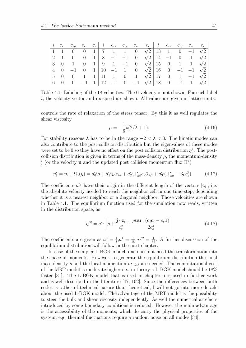
4.2. The lattice Boltzmann method 41
i cix ciy ciz ci i cix ciy ciz ci i cix ciy ciz ci
1 1 0 0 1 7 1 1 0√
2 13 1 0 −1√
2
2 1 0 0 1 8 −1 −1 0√
2 14 −1 0 1√
2
3 0 1 0 1 9 1 −1 0√
2 15 0 1 1√
2
4 0 −1 0 1 10 −1 1 0√
2 16 0 −1 −1√
2
5 0 0 1 1 11 1 0 1√
2 17 0 1 −1√
2
6 0 0 −1 1 12 −1 0 −1√
2 18 0 −1 1√
2
Table 4.1: Labeling of the 18-velocities. The 0-velocity is not shown. For each labeli, the velocity vector and its speed are shown. All values are given in lattice units.
controls the rate of relaxation of the stress tensor. By this it as well regulates theshear viscosity
µ = −1
6ρ(2/λ + 1). (4.16)
For stability reasons λ has to be in the range −2 < λ < 0. The kinetic modes canalso contribute to the post collision distribution but the eigenvalues of these modeswere set to be 0 so they have no effect on the post collision distribution η∗
i . The post-collision distribution is given in terms of the mass-density ρ, the momentum-densityj (or the velocity u and the updated post collision momentum flux Π∗)
η∗i = ηi + Ωi(η) = aci
0 ρ + aci1 jαciα + aci
2 Π∗αβ ¯ciαciβ + aci
3 (Π∗αα − 3ρc2
s). (4.17)
The coefficients acin have their origin in the different length of the vectors |ci|, i.e.
the absolute velocity needed to reach the neighbor cell in one time-step, dependingwhether it is a nearest neighbor or a diagonal neighbor. Those velocities are shownin Table 4.1. The equilibrium function used for the simulation now reads, writtenin the distribution space, as
ηeqi = aci
[
ρ +j · ci
c2s
+ρuu : (cici − cs1)
2c4s
]
(4.18)
The coefficients are given as a0 = 13,a1 = 1
18,a
√2 = 1
36. A further discussion of the
equilibrium distribution will follow in the next chapter.
In case of the simpler L-BGK model, one does not need the transformation intothe space of moments. However, to generate the equilibrium distribution the localmass density ρ and the local momentum m1,2,3 are needed. The computational costof the MRT model is moderate higher i.e., in theory a L-BGK model should be 18%faster [31]. The L-BGK model that is used in chapter 5 is used in further workand is well described in the literature [47, 102]. Since the differences between bothcodes is rather of technical nature than theoretical, I will not go into more detailsabout the used L-BGK model. The advantage of the MRT model is the possibilityto steer the bulk and shear viscosity independently. As well the numerical artefactsintroduced by some boundary conditions is reduced. However the main advantageis the accessibility of the moments, which do carry the physical properties of thesystem, e.g. thermal fluctuations require a random noise on all modes [34].
42 Chapter 4. Simulation method
4.2.4 From lattice Boltzmann to Navier-Stokes
After the presentation of the basic concept of the method it is now possible to showthat such a simplified form of the Boltzmann equation will reproduce fluid behavior.In this case it should be possible to perform a Chapman Enskog procedure andderive the Navier-Stokes equations
ρ
(
∂u
∂t+ (u∇u)
)
= −∆p + µ∇u + (λ + µ)∇(∇u), (4.19)
which can also be written in components as
∂tja + ∂β(ρc2sδαβ + ρuαuβ)∂β = σαβ. (4.20)
Einstein summation convention is in place, ∂α stands for ∂∂α
, the δαβ denotes aKronecker-δ. The viscous stress is given as
σαβ = µαβγδ∂γuδ, (4.21)
which in case of an isotropic fluid can be simplified by
µαβγδ = µ(δαγδβδ + δαδδβγ) + µvδαβδγδ (4.22)
with the shear viscosity µ and the bulk viscosity µv. We follow the standard asymp-totic analysis [57], like it is described in [35, 34, 68] for the lattice Boltzmann method.At first one introduces a dimensionless scaling parameter ǫ ≪ 1 and writes
x1 = ǫx. (4.23)
The idea behind this is to introduce a coarse-grained spatial resolution. In the sameway a coarse-grained time
t1 = ǫt (4.24)
is introduced. The reason to use the same ǫ for space and time is the wave-likepropagation of sound waves. However, to cover the momentum diffusion a secondcoarse-grained time scale
t2 = ǫ2t (4.25)
has to be introduced. Commonly ǫ is associated with the Knudsen number Kn thatdepicts the ratio of the mean free path of a molecule and the typical length scaleof the system. Another equivalent definition would be that the Knudsen numberis the ratio between the mean collision time of a molecule and the typical timescale of the hydrodynamic system. It is now possible to distinguish between thehydrodynamical short time scale ts = t1/ǫ and the hydrodynamical long time scaletl = t2/ǫ
2. Note that both time scales tl and ts are implicitly large on the latticescale, as it is the coarse-grained space. The hydrodynamic limit is reached for ǫ → 0meaning that the lattice space becomes much smaller than the typical length scale.However, it was shown that even a few lattice nodes are sufficient to reproduce fluidmechanic behavior [81, 105]. In this “multi-time scale” analysis, the populationdensity function η can be written in the coarse-grained coordinates
ηi ≡ ηi(x1, t1, t2) (4.26)
4.2. The lattice Boltzmann method 43
and the proceeding of the algorithm by a time step t → t + δt can be written ast1 → t1 + ǫδt and t2 → t2 + ǫ2δt. Thus, the LB-equation reads as
ηi(x1 + ǫt1ci, t1 + ǫδt, t2 + ǫ2δt) − ηi(x1, t1, t2) = Ωi (4.27)
It is assumed that the population density is a slowly varying function of the coarse-grained variables ξ = [x1, t1, t2]. A Taylor expansion of Eq. 4.27 reads as
ηi(ξ + δξ) = ηi(ξ) +∑
k
∂ηi
∂ξk
δξk +1
2
∑
kl
∂2ηi
∂ξk∂ξl
+ ... (4.28)
Since the collision operator Ω(ηi) depends on the distribution function ηi one has totake into account its ǫ dependence
ηi = η(0)i + ǫη
(1)i + O(ǫ2) (4.29)
Ωi = Ω(0)i + ǫΩ
(1)i + ǫ2Ω
(2)i + O(ǫ3). (4.30)
One can now apply the conservation laws that must hold independently of ǫ andtherefore on any order k one concludes that
∑
i
Ω(k)i =
∑
i
Ω(k)i ci = 0. (4.31)
By collecting the different orders of ǫ and implementing these relations to Eq. 4.27one obtains
Ω0i = 0, (4.32)
(∂t1 + ci · ∂x1)η(0)i =
1
δtΩ
(1)i , (4.33)
∂t2η(0)i +
δt
2(∂t1 + ci · ∂x1)
2η(0)i + (∂t1 + ci · ∂x1)η
(1)i =
1
δtΩ2
i . (4.34)
Using Eq. 4.33 one can now eliminate the second η(0)i in Eq. 4.34 so that
∂t2η(0)i +
1
2(∂t1 + ci · ∂x1)(η
∗(1)i + η
(1)i ) =
1
δtΩ
(2)i . (4.35)
with η∗i = ηi + Ωi being the post collision population in direction ci. The equations
above imply that the relaxation time scale of the collisions t ∼ δt, the sound propa-gation t ∼ δt/ǫ, and the momentum diffusion t ∼ δt/ǫ2, are separated and thereforeit is possible to calculate the collision operator of a higher order from the lowerorder one. One can as well conclude that the zeroth order of the collision operatorΩ
(0)i does only depend on η
(0)i . Further, Eq. 4.32 shows that η
(0)i is invariant under
collisions and therefore has to be the equilibrium distribution ηeqi . This implies that
the equilibrium distribution should depend only on conserved quantities, namelythe mass density ρ and the momentum density j. Otherwise, the algorithm wouldconserve physically not conserved quantities. Since there is no contribution fromhigher orders to the mass density ρ and the momentum density j one can expressthese quantities in terms of the equilibrium function
∑
i
ηeqi = ρ (4.36)
44 Chapter 4. Simulation method
and∑
i
ηeqi ci = j. (4.37)
This is concluded from the vanishing of the higher orders in mass and momentumdensity
0 = ρ(1) = ρ(0)...
and0 = j(1) = j(2)...
The higher orders vanish because otherwise η(0)i would have ǫ-dependent components
which would contradict Eq. 4.32.The dynamics of the LB-model on the longer time scales can now be gained by
analysing the moments of Eq. 4.33 and Eq. 4.35 with respect to the discrete veloc-ity set ci. From the previous chapter we know that the moments are carrying thephysical properties, so their dynamics are the point of interest. Hereby some con-ditions towards the collision operator Ωi become obvious. From the zeroth momentof Eq. 4.33 one obtains the continuum equation on the time scale t1:
∑
i
(∂t1 + ci · ∂x1)η(0)i =
∑
i
1
δtΩ
(1)i = (4.38)
∂t1 + ∂x1αjα = 0 (4.39)
and incompressibility on the time scale t2
∑
i
[
∂t2η(0)i +
1
2(∂t1 + ci · ∂x1)(η
∗(1)i + η
(1)i )
]
=∑
i
1
δtΩ
(2)i =
∂t2ρ +∑
i
1
2(∂t1 + ci · ∂x1)(η
∗(1)i + η
(1)i ) = 0 =
∂t2ρ = 0 (4.40)
Here one uses the condition that the collision operator may not change mass andmomentum density, and therefore each order of the collision operator Ω(n) = 0may not change the mass and momentum density. The first moment gives us themomentum conservation. Starting with Eq. 4.33 on the first time scale t1
∑
i
ci
[
(∂t1 + cj · ∂x1)η(0)i
]
=∑
i
ci
1
δtΩ
(1)i =
∂t1j + ∂x1
∑
i
cicjη0i = 0 (4.41)
and writing this in components ciα and with the momentum flux
Πα,β =∑
i
ηiciαciβ
one can write the momentum as
∂t1jα + ∂x1βΠ(0)αβ = 0. (4.42)

4.2. The lattice Boltzmann method 45
On the time scale t2 the momentum reads as
∑
i
ci
[
∂t2η(0)i +
1
2(∂t1 + cj · ∂x1)(η
∗(1)i + η
(1)i )
]
=∑
i
ci
1
δtΩ
(2)i =
∂t2j(0) +
1
2
(
∂t1(j∗(1) + j(1)) + (
∑
i
cicj∂(η∗(1)i + η
(1)i )
)
= 0, (4.43)
with j(1) = 0 and the definition of the momentum flux Π and written in components
∂t2jα +1
2∂x1β
(
Π∗(1)αβ + Π
(1)αβ
)
= 0. (4.44)
To reproduce the Navier Stokes equation 4.20 one needs to rewrite Eq. 4.42and Eq 4.44 as a combination in terms of the lattice-scale coordinates x = x1/ǫ,t = t1/ǫ = t2/ǫ
2. By using ∂α as component of ∂x one gets for the spatial derivatives
∂α = ǫ∂x1α
and for the time derivative∂t = ǫ∂t1 + ǫ2∂t2 .
Mass and momentum density in a combination reads on the lattice spacing as
∂tρ + ∂αjα = 0, (4.45)
∂tjα + ∂βΠ(0)αβ +
1
2∂β
(
Π∗(1)αβ + Π
(1)αβ
)
= 0. (4.46)
Looking at Eq. 4.46 it is possible to identify the different terms in the Navier-Stokesequation 4.20
∂tjα + ∂β(ρc2sδαβ + ρuαuβ) = ∂βσαβ
The time derivative ∂tjα is obvious. Further, Π(0)αβ is the equilibrium momentum flux
Πeqαβ and therefore unchanged by the collision operator and does depend only on ρ
and j. Therefore, it can be identified as the Euler stress
Π(0)αβ = Πeq
αβ = ρc2sδαβ + ρuαuβ. (4.47)
Here the ideal gas equation of state is implemented in the code (c.f. Eq. 4.14). Allthat is left is to identify the remaining non-equilibrium part with the viscous stress
1
2
(
Π∗(1)αβ + Π
(1)αβ
)
= −σαβ, (4.48)
which leads under the postulation of an isotropic liquid and with the definition fromEq 4.15 to a shear viscosity of
µ = ρc2sδt
(
1
λ+
1
2
)
(4.49)
and a bulk viscosity of
µv = ρc2sδt
(
2
3λv
+1
3
)
. (4.50)

46 Chapter 4. Simulation method
Since the time step δt is the natural time unit of the method it is commonly set to 1and is not written in a lot of publications. The same applies for the distance betweentwo lattice sites or the volume of one lattice node. For other collision operators orequilibrium functions several steps of this Chapman Enskog procedure have to beredone in an analogue way. Further, one can impose non ideal equations of stateor fluctuations, which makes the analysis more complicated. However, one can seethat the conservation of mass and momentum is inherently included in the latticeBoltzmann scheme and one only has to make sure that the viscous damping is donein a correct way.
4.2.5 External forces
External forces f are crucial to simulate fluid flow. In principal an external forcechanges the momentum of the fluid so one could naively just add it to the momentumjnew = jold + fδt in every time step δt. In the lattice Boltzmann scheme with discretetime this would rise the question at which time one has to add the forces or if itcan be done at any time. Therefore, it is useful to see the external forces as anadditional collision operator Ω′, so the lattice Boltzmann equation reads as
η∗i − ηi =
∑
j
Lij(ηj − ηeqj ) + Ω′
i. (4.51)
The additional collision operator Ω′ may not change the mass∑
i
Ω′i = 0, (4.52)
but has to change the momentum∑
i
Ω′ci = δtf . (4.53)
A consequence of this is that the momentum j is not any longer unique and any valuebetween
∑
i ciηi and∑
i ciηi + δtf could be correct. However, it was shown that awrongly assumed force could lead to unphysical behavior like negative permeabilitiesin porous-media [100]. Numerical [80] and theoretical [145] analysis have shownthat the optimum value is the arithmetic mean of pre and post collision momentum.Therefore, one defines the momentum density as
j =∑
i
ciηi + fδt
2. (4.54)
This has two consequences. First one has to keep this in mind when creating anoutput of the velocity. The second is that one needs the right flow velocity toconstruct the equilibrium function ηeq, so that the equilibrium momentum densityis equal to the defined one
∑
i
ηeqi ci = j, (4.55)
but the non-equilibrium part does not include the momentum change so that,
∑
i
ηneqi ci = −f
δt
2. (4.56)

4.2. The lattice Boltzmann method 47
If one would leave out the latter term and would just impose∑
i ηneqi ci = 0 as done
in [145] one would add a small error of order f 2 to the distribution. This leads tospurious terms in the Chapman-Enskog analysis, like a force dependent viscosity.This might become important in the case of strongly inhomogeneous forces but thedifferences vanish in the low Reynolds number limit. To be consistent with theforce-free case, one needs to adapt the relaxation of the non-equilibrium momentumflux in such a way that the resulting viscosity is the same as in the force free case.The resulting additional force collision operator with ciα = ci · eα then reads as
Ω′ = aci
[
δt
c2s
faciα +δt
2c4s
Σαβ(ciαciβ − c2sδαβ)
]
, (4.57)
with Σαβ containing the adaption of the non-equilibrium momentum flux. In thecode this is realized by adding half the force to the momentum then calculate theequilibrium distribution in the momentum space, relax the moments towards thisequilibrium and in the end add the remaining half of the force f
2and the momentum
flux correction
cαβ =1 + λ
2ρ(jαfβ + jβfα) (4.58)
to the corresponding moments.
4.2.6 Multi-phase models in lattice Boltzmann
One strength of the lattice Boltzmann method is the possibility to implement multi-phase and multi-component flow. For clarification the two cases will be distinguishedin this thesis as follows. Multi-component flow should be flow that contains many(usually two) distinguished liquids with potentially different chemical properties likewater and oil. Multi-phase (usually two phase) flow is a flow with distinguishablephases of the same component like liquid and vapor. It should be noted that for thiswork the actual phase transition is not of interest and a two phase model is usedto simulate bubbles attached to a surface or to model the wetting behavior of theboundary.
The Oxford model
The Oxford or free energy model was developed by Swift, Osborn and Yeomans[134, 133]. The main idea of the model is to have a well defined isothermal equationof state and force the system to equilibrate towards the desired state. Therefore,one defines a free energy as that of a van der Waals fluid
Ψ[ρ] =∫
[
k
2|∇ρ(r)|2 + ψ(ρ(r, T ))
]
dr, (4.59)
with ψ(ρ, T ) being the bulk free-energy density at temperature T
ψ(ρ, T ) = ηT ln
(
ρ
1 − ρb
)
− aρ2 (4.60)
48 Chapter 4. Simulation method
while the second term gives the free-energy contribution from the density gradientsin an inhomogeneous system. ρ =
∑
i ηi indicates the number of particles. Here, ais a measure for the attraction between the particles and b is the excluded volume.
With this free energy one is now able to construct an equilibrium distributionfunction ηeq
i that does not have an ideal gas equation of state. Therefore, the pressuretensor is related to the free energy
Pαβ(x) = p(x)δαβ + κ∂ρ
∂xα
∂ρ
∂xβ
, (4.61)
withp(x) = p0 − κη∇2ρ − κ
2|∇ρ|2, (4.62)
where
p0 = ρdψ(ρ)
dρ− ψ(ρ)
is the equation of state of the fluid. The actual equilibrium function depends onthe type of lattice and collision operator. Since the equation of state is forced onthe system from top one calls such a method a top down method. In the same wayone can find a free energy for a two component model or for the fluid-boundaryinteraction. Besides the studies of phase separation, Varnik et al. used such a modelto investigate the behavior of droplets on a surface [46].
The Shan-Chen model
Instead of imposing an equation of state and force the system towards it, it is possibleto introduce an internal force that models the intermolecular interactions. Such amodel was developed by Shan and Chen [124, 125, 126]. This force should simulatethe long range interactions between the particles. Therefore, one considers at asystem with S components and defines a potential of the form
V (x,x′) =S
∑
σ
S∑
σ
Gσσ(x,x′)Ψσ(ρσ(x))Ψσ(ρσ(x′)) (4.63)
where ρσ and ρσ are the number density of component σ and σ. Since the distancebetween two lattice points is fixed the number density determines the average particleparticle distance. Therefore, the potential is made to be the product of the local so-called effective masses Ψσ(ρσ) which are a function of the local densities ρσ only. Theexact form of Ψ is discussed latter. It determines the detailed interaction and theequation of state. The strength of the interaction is controlled by the Greens functionGσσ(x,x′). In case of a homogeneous system this is reduced to Gσσ(|x − x′|). In caseone takes into account only nearest and next nearest-neighbours one can reduce theGreens function in a one component system to a single number g. In case of a multi-component system one needs a symmetric tensor gσσ to steer the interaction betweeneach component. Depending whether gσσ is positive or negative the interaction isrepulsive or attractive. From the potential one can now derive a local force
fσσ = Ψσ(ρσ(x))gσσ
∑
i
ciΨσ(ρ(x + ci)). (4.64)
4.2. The lattice Boltzmann method 49
This force can now be included in a similar manner as external forces in the previoussection. Note that the force does not conserve the local momentum but in total nomomentum change is induced due to the symmetry of gσσ. Shan and Chen showedby performing a Chapman Enskog procedure that in case of a one component systemone can reproduce a Van der Waals like equation of state [124]. Here, it has to benoted that their analysis was done on a different lattice Boltzmann model than thetwo ones that are used in this thesis. However they showed that an effective mass of
Ψ(ρ) = 1 − e− ρ
ρ0 , (4.65)
with the reference density ρ0 can produce a non-monotonic pressure in dependenceof ρ. Therefore, a negative dp
dηappears in the equation of state, which corresponds
with a thermodynamic instability and the system segregates into a dense (liquid)and a light (gas) phase. However, typical density ratios between the dense and thelight phase are ρdense
ρlight= 40, so they are still far away from the ratio in real systems
where a typical density ratio would be ρdense
ρlight= 1000.
Nevertheless, one can achieve a phase separation between two components likewater and oil. To do so one needs an equilibrium function that includes the combinedvelocities of both species. The interaction Eq. 4.64 has the same form as for onecomponent but instead of gσσ one needs the non diagonal parts of gσσ. Since onehas only two components and one needs the symmetry this simply reads as a singlevalue gow which steers the interaction between the two species. Later it is shownthat such a force can as well be used to describe the wetting behavior of a solidboundary.
4.2.7 Solid-fluid boundary conditions
To simulate fluid flow in the presence of any solid object one needs to define bound-ary conditions at the interface between them. Further, it is a challenging task toimplement moving objects in a fluid solver like it has to be done for the simula-tion of the AFM based slip experiments. In the lattice Boltzmann scheme, findinga boundary condition means to find unknown population densities ηi that are notdefined because prior to the collision step they are lacking corresponding neighbors.This is depicted in Fig. 4.2 for a D2Q9 model.
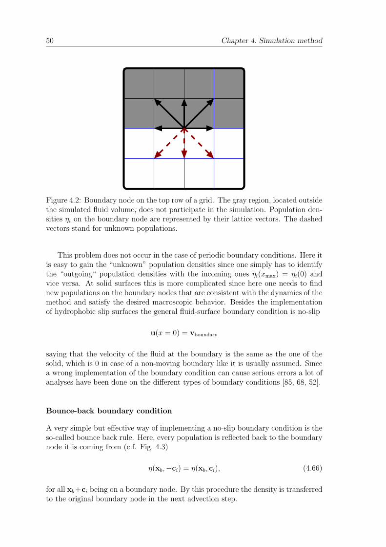
50 Chapter 4. Simulation method
Figure 4.2: Boundary node on the top row of a grid. The gray region, located outsidethe simulated fluid volume, does not participate in the simulation. Population den-sities ηi on the boundary node are represented by their lattice vectors. The dashedvectors stand for unknown populations.
This problem does not occur in the case of periodic boundary conditions. Here itis easy to gain the “unknown” population densities since one simply has to identifythe “outgoing“ population densities with the incoming ones ηi(xmax) = ηi(0) andvice versa. At solid surfaces this is more complicated since here one needs to findnew populations on the boundary nodes that are consistent with the dynamics of themethod and satisfy the desired macroscopic behavior. Besides the implementationof hydrophobic slip surfaces the general fluid-surface boundary condition is no-slip
u(x = 0) = vboundary
saying that the velocity of the fluid at the boundary is the same as the one of thesolid, which is 0 in case of a non-moving boundary like it is usually assumed. Sincea wrong implementation of the boundary condition can cause serious errors a lot ofanalyses have been done on the different types of boundary conditions [85, 68, 52].
Bounce-back boundary condition
A very simple but effective way of implementing a no-slip boundary condition is theso-called bounce back rule. Here, every population is reflected back to the boundarynode it is coming from (c.f. Fig. 4.3)
η(xb,−ci) = η(xb, ci), (4.66)
for all xb+ci being on a boundary node. By this procedure the density is transferredto the original boundary node in the next advection step.
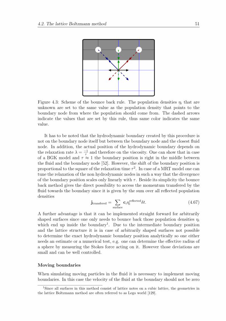
4.2. The lattice Boltzmann method 51
Figure 4.3: Scheme of the bounce back rule. The population densities ηi that areunknown are set to the same value as the population density that points to theboundary node from where the population should come from. The dashed arrowsindicate the values that are set by this rule, thus same color indicates the samevalue.
It has to be noted that the hydrodynamic boundary created by this procedure isnot on the boundary node itself but between the boundary node and the closest fluidnode. In addition, the actual position of the hydrodynamic boundary depends onthe relaxation rate λ = −1
τand therefore on the viscosity. One can show that in case
of a BGK model and τ ≈ 1 the boundary position is right in the middle betweenthe fluid and the boundary node [52]. However, the shift of the boundary position isproportional to the square of the relaxation time τ 2. In case of a MRT model one cantune the relaxation of the non hydrodynamic nodes in such a way that the divergenceof the boundary position scales only linearly with τ . Beside its simplicity the bounceback method gives the direct possibility to access the momentum transfered by thefluid towards the boundary since it is given by the sum over all reflected populationdensities
jtransfered =∑
surface
ciηreflectedi δt. (4.67)
A further advantage is that it can be implemented straight forward for arbitrarilyshaped surfaces since one only needs to bounce back those population densities ηi
which end up inside the boundary1. Due to the intermediate boundary positionand the lattice structure it is in case of arbitrarily shaped surfaces not possibleto determine the exact hydrodynamic boundary position analytically so one eitherneeds an estimate or a numerical test, e.g. one can determine the effective radius ofa sphere by measuring the Stokes force acting on it. However those deviations aresmall and can be well controlled.
Moving boundaries
When simulating moving particles in the fluid it is necessary to implement movingboundaries. In this case the velocity of the fluid at the boundary should not be zero
1Since all surfaces in this method consist of lattice notes on a cubic lattice, the geometries inthe lattice Boltzmann method are often referred to as Lego world [129].
52 Chapter 4. Simulation method
compared to the lattice but be the velocity of the boundary. In the given simulationthis is realized by a generalization of the bounce back boundary condition, whichtakes into account the momentum of the moving object. The method was developedby Ladd et al. and described extensively in the literature [145]. The picture oneshould have in mind is that an ensemble of particles moving with the velocity ci
is hitting a perpendicular wall which is moving with velocity vb ≪ ci. After theparticles hit the wall their velocity is −ci + 2vb and the force exerted on the wallis proportional to ci − vb. Since the velocities in the lattice Boltzmann scheme arediscrete, such a scheme cannot be implemented directly but one has to modify thedensity of the bounced back particles such that the transfered momentum equalsthe same as in the continuous case.
At first one takes into account those population densities η(xb, cb, t) close to theboundary of the object for those cb that xb +cbδt is a solid node. This is the same asin the normal bounce back method. One now defines a simple rule for the unknown“bounced back” particles η(xb,−cb, t + δt) that takes into account the movement ofthe boundary
η(xb,−cb, t + δt) = η∗(xb, cb, t) −2acbρvb · cb
c2s
. (4.68)
η∗(xb, cb, t) is the post collision distribution population. The local velocity of thesurface is vb, which takes into account the center of mass velocity and the angularvelocity of the particle. However, in the cases that are of interest in this thesis theangular velocity is kept to 0 so that vb is the center of mass velocity of the object.The force acting on the object can be calculated from the total momentum exchangebetween the fluid and all of its boundary nodes.
Due to the lattice nature of the lattice Boltzmann method one needs to placeparticles on the grid. Therefore, the shape of the particle is estimated by the latticenodes that are mainly inside the particle. Such an approximation seams very roughbut even at small radii like 2.5 lattice units, the error in the hydrodynamic interactioncan be kept within 1% of an exact numerical solution [22]. This will be validatedlatter in this thesis.
Particle motion
The movement of the particles themselves is realized like in a molecular dynamics(MD) simulation, i.e., one calculates the forces acting on the particle and changesits velocity afterwards. In contrast to a classical MD simulation the force is notcoming from pairwise potentials but from the hydrodynamic interaction. The im-plementation of such potentials would be straightforward but so far only a hardsphere potential between particles is implemented. Further, it should be noted thatthe velocity in the presented simulations is kept constant by setting the mass of theparticle to infinity. The infinite mass is important for the force measurement be-cause in this case the velocity in Eq. 4.68 is vb(t + δt
2) as it is used in the underlying
velocity Verlet integration2. One has to make sure that vb(t + δt2) is constant even
if a force acts on the sphere. After the center of mass movement is calculated onemight have to change the occupied lattice nodes. This update of nodes is not a
2sounds easy but can cost you one year...

4.2. The lattice Boltzmann method 53
continuous motion but a discrete jumping over the lattice. Due to this jumping theflow field (and therefore the forces) around the particles need some time to cometo an quasi-equilibrium. For the practical use this means that one has to averageforces over several time steps. Further, it limits this method to low Mach numbers,since one should change the boundary node configuration only after one has a wellaveraged value for the given configuration. However, the equilibration takes onlyabout 10 time steps so that this condition is relatively easy to be fulfilled.
Hydrophobic boundaries
It is known from MD-simulations that the interaction between the boundary and thefluid causing a slip phenomenon usually takes place within a few molecular layers ofthe liquid along the boundary surface [136, 135, 71, 23, 72, 24, 5].
The implementation of solid hydrophobic boundaries contains two parts. Sincesuch a boundary consists of a solid wall one implements a bounce back boundarycondition. The second part covers the hydrophobic interaction between the bound-ary and the fluid. It is realized in the same way as the interaction between twocomponents in a multi-component system (c.f. the previous section). In our casea Shan Chen like force fwf between the fluid nodes close to the boundary and theboundary nodes itself is implemented. Such a force reads as
fwf (x) = Ψfluid(x)∑
i
cigwfΨwall(x + ci). (4.69)
The force is in full analogy to Eq: 4.64. The effective mass of the boundaryΨwall = 1 − exp(−ρwall/ρ0) is a local parameter that indicates how strong the localhydrophobic interaction is while gwf is a global coupling parameter. It is as wellpossible to assign a virtual ”fluid density” to a boundary node. By this one canuse a one component multi-phase Shan Chen model to simulate the solid-fluid in-teractions and a possible phase-transition close to the boundary as it happens atsuper-hydrophobic surfaces.
Further, a hydrophobic interaction like the presented one can be utilized to modelapparent slip [48, 76, 49, 117]. Due to the repellent hydrodynamic force, a depletionlayer close to the boundary is formed where the fluid density ρ and therefore theviscosity µ is reduced. This viscosity reduction finally leads to apparent slip. Thedependences are discussed in section 4.2.8.
Alternative boundary conditions
Besides the presented boundary conditions there are many other possible implemen-tations. Most of them have a higher precision than the simple bounce back rulebut might have to take into account more boundary nodes, which makes them non-local, or they are not able to handle arbitrary geometries. Further, not all proposedboundary conditions can be applied on a 3D lattice. An overview over differentboundaries was recently published by Latt et al. [85].
One possible solution is to create the missing populations by assuming that theyfollow the equilibrium distribution with the given velocity. In this case one still hasto find a corresponding pressure (or density) at the close boundary nodes [62].
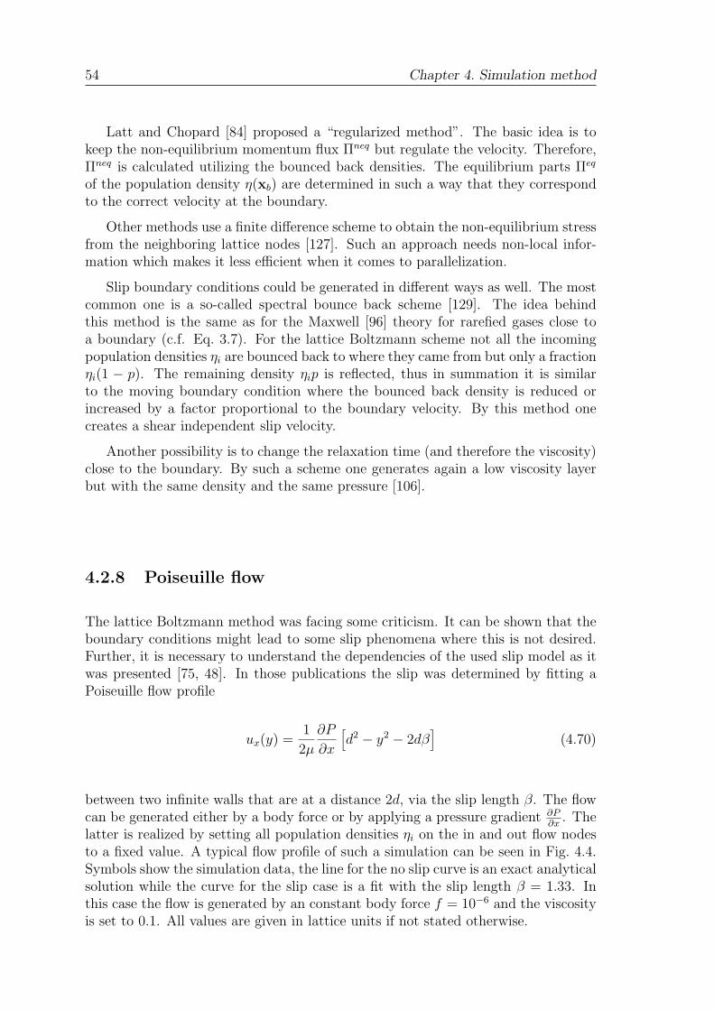
54 Chapter 4. Simulation method
Latt and Chopard [84] proposed a “regularized method”. The basic idea is tokeep the non-equilibrium momentum flux Πneq but regulate the velocity. Therefore,Πneq is calculated utilizing the bounced back densities. The equilibrium parts Πeq
of the population density η(xb) are determined in such a way that they correspondto the correct velocity at the boundary.
Other methods use a finite difference scheme to obtain the non-equilibrium stressfrom the neighboring lattice nodes [127]. Such an approach needs non-local infor-mation which makes it less efficient when it comes to parallelization.
Slip boundary conditions could be generated in different ways as well. The mostcommon one is a so-called spectral bounce back scheme [129]. The idea behindthis method is the same as for the Maxwell [96] theory for rarefied gases close toa boundary (c.f. Eq. 3.7). For the lattice Boltzmann scheme not all the incomingpopulation densities ηi are bounced back to where they came from but only a fractionηi(1 − p). The remaining density ηip is reflected, thus in summation it is similarto the moving boundary condition where the bounced back density is reduced orincreased by a factor proportional to the boundary velocity. By this method onecreates a shear independent slip velocity.
Another possibility is to change the relaxation time (and therefore the viscosity)close to the boundary. By such a scheme one generates again a low viscosity layerbut with the same density and the same pressure [106].
4.2.8 Poiseuille flow
The lattice Boltzmann method was facing some criticism. It can be shown that theboundary conditions might lead to some slip phenomena where this is not desired.Further, it is necessary to understand the dependencies of the used slip model as itwas presented [75, 48]. In those publications the slip was determined by fitting aPoiseuille flow profile
ux(y) =1
2µ
∂P
∂x
[
d2 − y2 − 2dβ]
(4.70)
between two infinite walls that are at a distance 2d, via the slip length β. The flowcan be generated either by a body force or by applying a pressure gradient ∂P
∂x. The
latter is realized by setting all population densities ηi on the in and out flow nodesto a fixed value. A typical flow profile of such a simulation can be seen in Fig. 4.4.Symbols show the simulation data, the line for the no slip curve is an exact analyticalsolution while the curve for the slip case is a fit with the slip length β = 1.33. Inthis case the flow is generated by an constant body force f = 10−6 and the viscosityis set to 0.1. All values are given in lattice units if not stated otherwise.
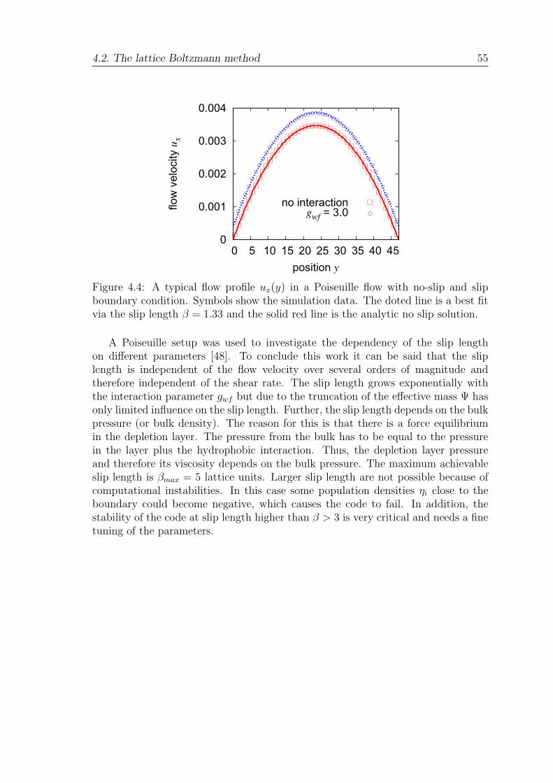
4.2. The lattice Boltzmann method 55
0
0.001
0.002
0.003
0.004
0 5 10 15 20 25 30 35 40 45
flo
w v
elo
city u
x
position y
no interactiongwf = 3.0
Figure 4.4: A typical flow profile ux(y) in a Poiseuille flow with no-slip and slipboundary condition. Symbols show the simulation data. The doted line is a best fitvia the slip length β = 1.33 and the solid red line is the analytic no slip solution.
A Poiseuille setup was used to investigate the dependency of the slip lengthon different parameters [48]. To conclude this work it can be said that the sliplength is independent of the flow velocity over several orders of magnitude andtherefore independent of the shear rate. The slip length grows exponentially withthe interaction parameter gwf but due to the truncation of the effective mass Ψ hasonly limited influence on the slip length. Further, the slip length depends on the bulkpressure (or bulk density). The reason for this is that there is a force equilibriumin the depletion layer. The pressure from the bulk has to be equal to the pressurein the layer plus the hydrophobic interaction. Thus, the depletion layer pressureand therefore its viscosity depends on the bulk pressure. The maximum achievableslip length is βmax = 5 lattice units. Larger slip length are not possible because ofcomputational instabilities. In this case some population densities ηi close to theboundary could become negative, which causes the code to fail. In addition, thestability of the code at slip length higher than β > 3 is very critical and needs a finetuning of the parameters.

56 Chapter 4. Simulation method
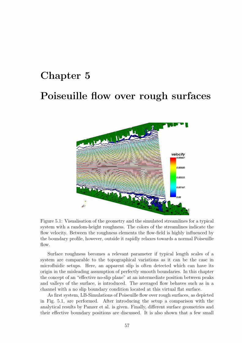
Chapter 5
Poiseuille flow over rough surfaces
Figure 5.1: Visualisation of the geometry and the simulated streamlines for a typicalsystem with a random-height roughness. The colors of the streamlines indicate theflow velocity. Between the roughness elements the flow-field is highly influenced bythe boundary profile, however, outside it rapidly relaxes towards a normal Poiseuilleflow.
Surface roughness becomes a relevant parameter if typical length scales of asystem are comparable to the topographical variations as it can be the case inmicrofluidic setups. Here, an apparent slip is often detected which can have itsorigin in the misleading assumption of perfectly smooth boundaries. In this chapterthe concept of an “effective no-slip plane” at an intermediate position between peaksand valleys of the surface, is introduced. The averaged flow behaves such as in achannel with a no slip boundary condition located at this virtual flat surface.
As first system, LB-Simulations of Poiseuille flow over rough surfaces, as depictedin Fig. 5.1, are performed. After introducing the setup a comparison with theanalytical results by Panzer et al. is given. Finally, different surface geometries andtheir effective boundary positions are discussed. It is also shown that a few small
57
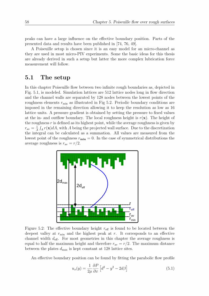
58 Chapter 5. Poiseuille flow over rough surfaces
peaks can have a large influence on the effective boundary position. Parts of thepresented data and results have been published in [74, 76, 49].
A Poiseuille setup is chosen since it is an easy model for an micro-channel asthey are used in most micro-PIV experiments. Some the basic ideas for this thesisare already derived in such a setup but latter the more complex lubrication forcemeasurement will follow.
5.1 The setup
In this chapter Poiseuille flow between two infinite rough boundaries as, depicted inFig. 5.1, is modeled. Simulation lattices are 512 lattice nodes long in flow directionand the channel walls are separated by 128 nodes between the lowest points of theroughness elements rmin as illustrated in Fig 5.2. Periodic boundary conditions areimposed in the remaining direction allowing it to keep the resolution as low as 16lattice units. A pressure gradient is obtained by setting the pressure to fixed valuesat the in- and outflow boundary. The local roughness height is r(x). The height ofthe roughness r is defined as its highest point, while the average roughness is given byrav = 1
A
∫
A r(x)dA, with A being the projected wall surface. Due to the discretizationthe integral can be calculated as a summation. All values are measured from thelowest point of the roughness rmin = 0. In the case of symmetrical distributions theaverage roughness is rav = r/2.
r
r
r
2deff
2dmax
min
av
effr
Figure 5.2: The effective boundary height reff is found to be located between thedeepest valley at rmin and the highest peak at r. It corresponds to an effectivechannel width deff . For most geometries in this chapter the average roughness isequal to half the maximum height and therefore rav = r/2. The maximum distancebetween the plates dmax is kept constant at 128 lattice sites.
An effective boundary position can be found by fitting the parabolic flow profile
ux(y) =1
2µ
∂P
∂x
[
d2 − y2 − 2dβ]
(5.1)
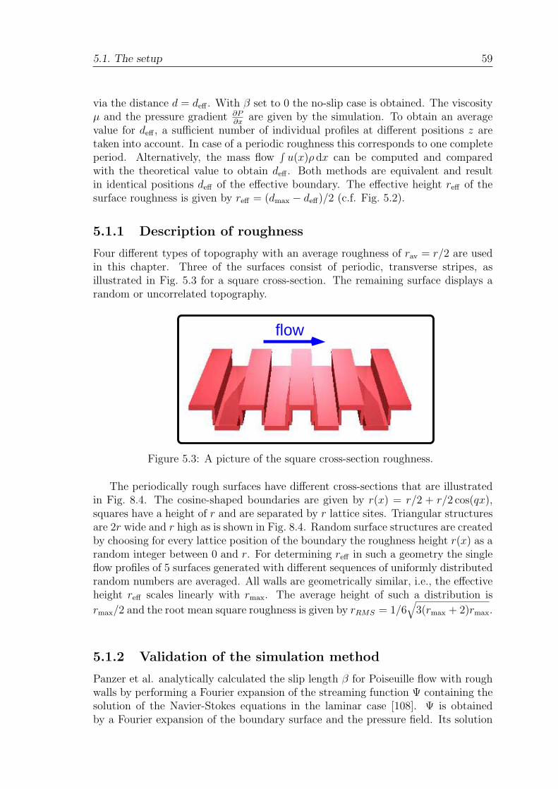
5.1. The setup 59
via the distance d = deff . With β set to 0 the no-slip case is obtained. The viscosityµ and the pressure gradient ∂P
∂xare given by the simulation. To obtain an average
value for deff , a sufficient number of individual profiles at different positions z aretaken into account. In case of a periodic roughness this corresponds to one completeperiod. Alternatively, the mass flow
∫
u(x)ρ dx can be computed and comparedwith the theoretical value to obtain deff . Both methods are equivalent and resultin identical positions deff of the effective boundary. The effective height reff of thesurface roughness is given by reff = (dmax − deff)/2 (c.f. Fig. 5.2).
5.1.1 Description of roughness
Four different types of topography with an average roughness of rav = r/2 are usedin this chapter. Three of the surfaces consist of periodic, transverse stripes, asillustrated in Fig. 5.3 for a square cross-section. The remaining surface displays arandom or uncorrelated topography.
flow
Figure 5.3: A picture of the square cross-section roughness.
The periodically rough surfaces have different cross-sections that are illustratedin Fig. 8.4. The cosine-shaped boundaries are given by r(x) = r/2 + r/2 cos(qx),squares have a height of r and are separated by r lattice sites. Triangular structuresare 2r wide and r high as is shown in Fig. 8.4. Random surface structures are createdby choosing for every lattice position of the boundary the roughness height r(x) as arandom integer between 0 and r. For determining reff in such a geometry the singleflow profiles of 5 surfaces generated with different sequences of uniformly distributedrandom numbers are averaged. All walls are geometrically similar, i.e., the effectiveheight reff scales linearly with rmax. The average height of such a distribution is
rmax/2 and the root mean square roughness is given by rRMS = 1/6√
3(rmax + 2)rmax.
5.1.2 Validation of the simulation method
Panzer et al. analytically calculated the slip length β for Poiseuille flow with roughwalls by performing a Fourier expansion of the streaming function Ψ containing thesolution of the Navier-Stokes equations in the laminar case [108]. Ψ is obtainedby a Fourier expansion of the boundary surface and the pressure field. Its solution
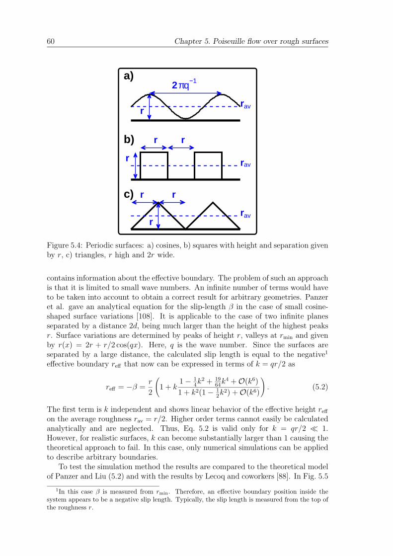
60 Chapter 5. Poiseuille flow over rough surfaces
r r
r r
2πq−1
r
r
r
av
av
avr
r
r
a)
b)
c)
Figure 5.4: Periodic surfaces: a) cosines, b) squares with height and separation givenby r, c) triangles, r high and 2r wide.
contains information about the effective boundary. The problem of such an approachis that it is limited to small wave numbers. An infinite number of terms would haveto be taken into account to obtain a correct result for arbitrary geometries. Panzeret al. gave an analytical equation for the slip-length β in the case of small cosine-shaped surface variations [108]. It is applicable to the case of two infinite planesseparated by a distance 2d, being much larger than the height of the highest peaksr. Surface variations are determined by peaks of height r, valleys at rmin and givenby r(x) = 2r + r/2 cos(qx). Here, q is the wave number. Since the surfaces areseparated by a large distance, the calculated slip length is equal to the negative1
effective boundary reff that now can be expressed in terms of k = qr/2 as
reff = −β =r
2
(
1 + k1 − 1
4k2 + 19
64k4 + O(k6)
1 + k2(1 − 12k2) + O(k6)
)
. (5.2)
The first term is k independent and shows linear behavior of the effective height reff
on the average roughness rav = r/2. Higher order terms cannot easily be calculatedanalytically and are neglected. Thus, Eq. 5.2 is valid only for k = qr/2 ≪ 1.However, for realistic surfaces, k can become substantially larger than 1 causing thetheoretical approach to fail. In this case, only numerical simulations can be appliedto describe arbitrary boundaries.
To test the simulation method the results are compared to the theoretical modelof Panzer and Liu (5.2) and with the results by Lecoq and coworkers [88]. In Fig. 5.5
1In this case β is measured from rmin. Therefore, an effective boundary position inside thesystem appears to be a negative slip length. Typically, the slip length is measured from the top ofthe roughness r.
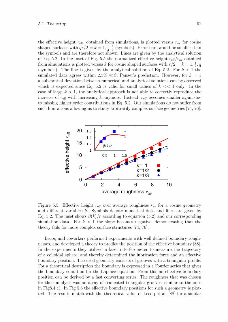
5.1. The setup 61
the effective height reff , obtained from simulations, is plotted versus rav for cosineshaped surfaces with qr/2 = k = 1, 1
2, 1
3(symbols). Error bars would be smaller than
the symbols and are therefore not shown. Lines are given by the analytical solutionof Eq. 5.2. In the inset of Fig. 5.5 the normalized effective height reff/rav obtainedfrom simulations is plotted versus k for cosine shaped surfaces with r/2 = k = 1, 1
2, 1
3
(symbols). The line is given by the analytical solution of Eq. 5.2. For k < 1 thesimulated data agrees within 2.5% with Panzer’s prediction. However, for k = 1a substantial deviation between numerical and analytical solutions can be observedwhich is expected since Eq. 5.2 is valid for small values of k << 1 only. In thecase of large k > 1, the analytical approach is not able to correctly reproduce theincrease of reff with increasing k anymore. Instead, reff becomes smaller again dueto missing higher order contributions in Eq. 5.2. Our simulations do not suffer fromsuch limitations allowing us to study arbitrarily complex surface geometries [74, 76].
0
5
10
15
20
0 2 4 6 8 10
effective h
eig
ht
r eff
average roughness rav
k= 1 k=1/2k=1/3
1
1.2
1.4
1.6
0.5 1 1.5
β(k)/r
Figure 5.5: Effective height reff over average roughness rav for a cosine geometryand different variables k. Symbols denote numerical data and lines are given byEq. 5.2. The inset shows β(k)/r according to equation (5.2) and our correspondingsimulation data. For k > 1 the slope becomes negative, demonstrating that thetheory fails for more complex surface structures [74, 76].
Lecoq and coworkers performed experiments with well defined boundary rough-nesses, and developed a theory to predict the position of the effective boundary [88].In the experiments they utilised a laser interferometer to measure the trajectoryof a colloidal sphere, and thereby determined the lubrication force and an effectiveboundary position. The used geometry consists of grooves with a triangular profile.For a theoretical description the boundary is expressed in a Fourier series that givesthe boundary condition for the Laplace equation. From this an effective boundaryposition can be derived by a fast converting series. The roughness that was chosenfor their analysis was an array of truncated triangular grooves, similar to the onesin Fig8.4 c). In Fig 5.6 the effective boundary positions for such a geometry is plot-ted. The results match with the theoretical value of Lecoq et al. [88] for a similar

62 Chapter 5. Poiseuille flow over rough surfaces
geometry.
0
2
4
6
8
10
12
14
16
18
0 1 2 3 4 5 6 7 8 9
effective h
eig
ht
r eff
average roughness rav
trianglesLecoq et al
Figure 5.6: Simulated effective height reff versus rav for triangular shaped grooves.The triangular shape matches the theoretical and experimentally validated resultsof Lecoq et al. [88] for a similar geometry that is plotted as dotted line [49].
A major problem of an analytical approach is that it can only be applied for sur-faces that can be well expressed by Fourier-series. Since one needs an infinitely highorders, to describe arbitrary surfaces, it is not possible to express them analyticallyand thus numerical solutions are needed [83].
5.2 Results
5.2.1 Model roughness
In Fig. 5.7 reff is plotted versus rav for the different types of roughness discussed inthe previous section. By performing a linear fit to the data as given by the linesone finds for the uniformly randomly distributed roughness that the position of theeffective wall is at reff = 1.84rav with rav = r/2 or in other words at 92% of themaximum height r.
For squares and triangular structures the constants of proportionality are foundto be c = 1.90 and c = 1.69 indicating that the shape of the surface variations indeedaffects the position of the effective boundary. However, the effect of the shape issmall compared to the effect of the height of the variations. All surface structuresare geometrically similar causing the linear dependence between reff and rav = r/2and c to be independent of the lattice resolution.
When converting the 3D random roughness into a purely 2D structure, the dif-ference in the measured constant of proportionality c is in the range of the error ofthe fit algorithm. This is a surprising result since in 3D the flow can pass sidewisearound a roughness element. The measured reff is found to be independent of the

5.2. Results 63
0
4
8
12
16
0 1 2 3 4 5 6 7 8 9
effe
ctiv
e he
ight
ref
f
average roughness rav
trianglesblocks
random
Figure 5.7: Effective height reff versus rav for triangles, blocks (see Fig. 8.4), and anequally distributed random roughness. Lines are a linear fit to the simulated datawith slopes 1.90, 1.69, and 1.84.
flow velocity over more than 3 decades and does not depend on pressure either, i.e.,reff is independent of the Reynolds number.
Non symmetric surface topology
In reality high spikes on a smooth surface may occur, so that the average roughnessrav is much smaller than half the maximum height r/2. This can be modeled by atriangular geometry with additional void space a between the roughness elements.As shown in the previous paragraph, the actual shape of the roughness elements hasonly a minor influence. However, the ratio a/r should have an influence, as longas a is sufficiently large. In this paragraph values of r = 5 and r = 10 lattice sitesare chosen to be the maximum height of the roughness. Similarly to Fig. 5.7 theeffective surface height reff over the average roughness rav is plotted in Fig. 5.8. It isapparent that the average roughness is smaller than one half of the maximum heightr/2, i.e., rav = r2
2r+a≤ r/2. The values of r = 5 are scaled by a factor of two to
be comparable with the values of r = 10. Due to the geometrical similarity of thesurface structure this scaling is possible. For comparison with Fig. 5.7 the linearfit with slope c = 1.69 is plotted. As can be seen in Fig. 5.8, for spaced roughnesselements, the maximum height r has a strong influence on the effective height reff
while the spacing a does not. For small values of rav (due to large additional distancea), which is corresponding to a flat surface, the effective height reff converges tozero. For small a the effective height reff converges to the same value as the trianglegeometry, as given in Fig. 5.7. For intermediate values of a ≈ 2hmax the effectiveboundary position is still in the range of 75% of the maximum height r. This isan important result, since it demonstrates that the distance between the effectiveboundary position reff and the lowest surface parts rmin can be much larger than theaverage roughness height rav. In such cases reff > 6 · rav can be obtained. On the

64 Chapter 5. Poiseuille flow over rough surfaces
other hand, for large a this results in heff < 0.7 · r. Therefore, in the case of largea ≈ 2r, the effective height reff cannot be approximated by the maximum heightrmax nor by the average roughness rav.
0
2
4
6
8
10
0 1 2 3 4 5
effe
ctiv
e he
ight
ref
f
average roughness rav
r=10r= 5
Figure 5.8: reff versus rav for triangles with r = 5 and 10. The distance betweentriangles a is varied to obtain the given rav. Values of r = 5 are scaled by a factorof 2 so one would see possible discretization effects. The fitted values for a trianglegeometry are shown as dotted line.
5.2.2 Flow over a realistic surface
An advantage of the lattice Boltzmann method over other CFD-methods is that non-trivial boundary-structures can easily be implemented. It is for example possible touse experimentally measured surfaces like the ones obtained from AFM data of agold coated glass surface which have been used in microflow experiments by O.I.Vinogradova and G.E. Yakubov [150]. The sample size is 1µm2 represented by512×512 data points with a maximum peak to valley distance of 64nm. The latticeconstant of the LB simulation can be scaled to 1.9nm by setting the relaxation time τto 1.15 and by mapping the speed of sound and the kinematic viscosity to the valuesfor water (cs = 1.5 · 103m/s, ν = 1.02 · 10−6m2/s). reff can then be measured asdescribed in the previous paragraphs by loading the AFM data onto our simulationlattice. For the simulations presented in this paragraph, the channel width is setto 128 lattice units. The effective height, obtained by the simulation of Poiseuileflow over the gold surface, is depicted by the square at rav=21nm in Fig. 5.9. Datapoints at rav = 4 and 8 are obtained by downscaling the original data set with aconstant factor. By analysing the surface data it is found that the distribution ofsurface heights follows a Gaussian distribution. This distribution is used to generatean artificial random surface with identical height distribution. To generate thisheight distribution a Gaussian-distributed random height for every lattice point onthe surface is obtained from a Box-Muller based algorithm [14]. The width of thedistribution σ and the average height rav can be set. By using the same sequence of
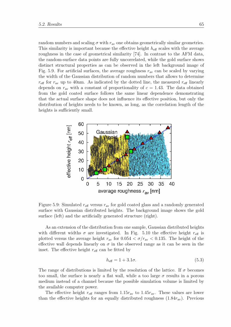
5.2. Results 65
random numbers and scaling σ with rav one obtains geometrically similar geometries.This similarity is important because the effective height heff scales with the averageroughness in the case of geometrical similarity [74]. In contrast to the AFM data,the random-surface data points are fully uncorrelated, while the gold surface showsdistinct structural properties as can be observed in the left background image ofFig. 5.9. For artificial surfaces, the average roughness rav can be scaled by varyingthe width of the Gaussian distribution of random numbers that allows to determinereff for rav up to 40nm. As indicated by the dotted line, the measured reff linearlydepends on rav with a constant of proportionality of c = 1.43. The data obtainedfrom the gold coated surface follows the same linear dependence demonstratingthat the actual surface shape does not influence its effective position, but only thedistribution of heights needs to be known, as long, as the correlation length of theheights is sufficiently small.
Figure 5.9: Simulated reff versus rav for gold coated glass and a randomly generatedsurface with Gaussian distributed heights. The background image shows the goldsurface (left) and the artificially generated structure (right).
As an extension of the distribution from one sample, Gaussian distributed heightswith different widths σ are investigated. In Fig. 5.10 the effective height reff isplotted versus the average height rav for 0.054 < σ/rav < 0.135. The height of theeffective wall depends linearly on σ in the observed range as it can be seen in theinset. The effective height reff can be fitted by
heff = 1 + 3.1σ. (5.3)
The range of distributions is limited by the resolution of the lattice. If σ becomestoo small, the surface is nearly a flat wall, while a too large σ results in a porousmedium instead of a channel because the possible simulation volume is limited bythe available computer power.
The effective height reff ranges from 1.15rav to 1.45rav. These values are lowerthan the effective heights for an equally distributed roughness (1.84rav). Previous
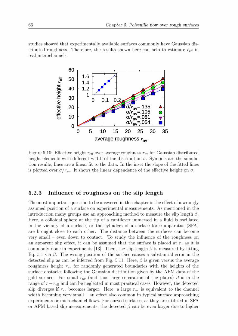
66 Chapter 5. Poiseuille flow over rough surfaces
studies showed that experimentally available surfaces commonly have Gaussian dis-tributed roughness. Therefore, the results shown here can help to estimate reff inreal microchannels.
0
10
20
30
40
50
60
0 5 10 15 20 25 30 35
effe
ctiv
e he
ight
ref
f
average roughness rav
σ/rav=.135σ/rav=.105σ/rav=.081σ/rav=.054
0
10
20
30
40
50
60
0 5 10 15 20 25 30 35
effe
ctiv
e he
ight
ref
f
average roughness rav
σ/rav=.135σ/rav=.105σ/rav=.081σ/rav=.054
1 1.2 1.4 1.6
0 0.1 0.2
Figure 5.10: Effective height reff over average roughness rav for Gaussian distributedheight elements with different width of the distribution σ. Symbols are the simula-tion results, lines are a linear fit to the data. In the inset the slope of the fitted linesis plotted over σ/rav. It shows the linear dependence of the effective height on σ.
5.2.3 Influence of roughness on the slip length
The most important question to be answered in this chapter is the effect of a wronglyassumed position of a surface on experimental measurements. As mentioned in theintroduction many groups use an approaching method to measure the slip length β.Here, a colloidal sphere at the tip of a cantilever immersed in a fluid is oscillatedin the vicinity of a surface, or the cylinders of a surface force apparatus (SFA)are brought close to each other. The distance between the surfaces can becomevery small – even down to contact. To study the influence of the roughness onan apparent slip effect, it can be assumed that the surface is placed at r, as it iscommonly done in experiments [13]. Then, the slip length β is measured by fittingEq. 5.1 via β. The wrong position of the surface causes a substantial error in thedetected slip as can be inferred from Fig. 5.11. Here, β is given versus the averageroughness height rav for randomly generated boundaries with the heights of thesurface obstacles following the Gaussian distribution given by the AFM data of thegold surface. For small rav (and thus large separation of the plates) β is in therange of r− reff and can be neglected in most practical cases. However, the detectedslip diverges if rav becomes larger. Here, a large rav is equivalent to the channelwidth becoming very small – an effect also common in typical surface approachingexperiments or microchannel flows. For curved surfaces, as they are utilized in SFAor AFM based slip measurements, the detected β can be even larger due to higher

5.3. Rough hydrophobic surfaces 67
order components of the flow field. This might explain experiments reporting largeslip lengths of β ≈ 100nm [86, 104].
0
20
40
60
80
100
0 10 20 30 40 50 60
slip
leng
th β
[nm
]
average roughness rav [nm]
Figure 5.11: β versus rav for water and randomly distributed roughness. By assumingreff = r, β is in the range of r − reff for small rav, but diverges for large rav.
5.3 Rough hydrophobic surfaces
A further interesting point in this chapter is how roughness and the surface wetta-bility act together. In order to study this interplay, simulation results are presentedfor a setup of rough channels including a fluid-wall interaction force. This force issimilar to a Shan-Chen force, as presented in chapter 4. As reminder it is statedhere that the Shan-Chen force is a repulsive force
fw,f (xj) = Ψ (ρ(xj)) gwfci
∑
Ψ (ρw(xj + ci)) ,
which leads to a depletion zone on the fluid nodes neighboring the boundary. Dueto this depletion the dynamic viscosity in this zone is lowered and therefore anapparent slip can be measured. The steering parameters of the slip length are thelocal wall density ρw and the global interaction parameter which is kept constantat gwf = 0.08. For a more detailed explanation see chapter 4 or the literature [48].For the wall density values of ρwall 0.5, 1, and 5 are chosen. For these values andperfectly smooth surfaces the slip length β has been determined to be 0.65, 1.13, and1.3, respectively. The roughness is composed of equally distributed random heights,so that rav = r/2. In order to obtain better results the values obtained from fourdifferent seeds of the random number generator are averaged. The seed determinesthe sequence of random numbers and therefore the actual shape of the boundarybut not the macroscopic properties, since the averaged parameters are left constant.
When analysing the effective height of rough hydrophobic walls in dependenceof the average roughness rav we find for rav > 4 a linear dependence between the
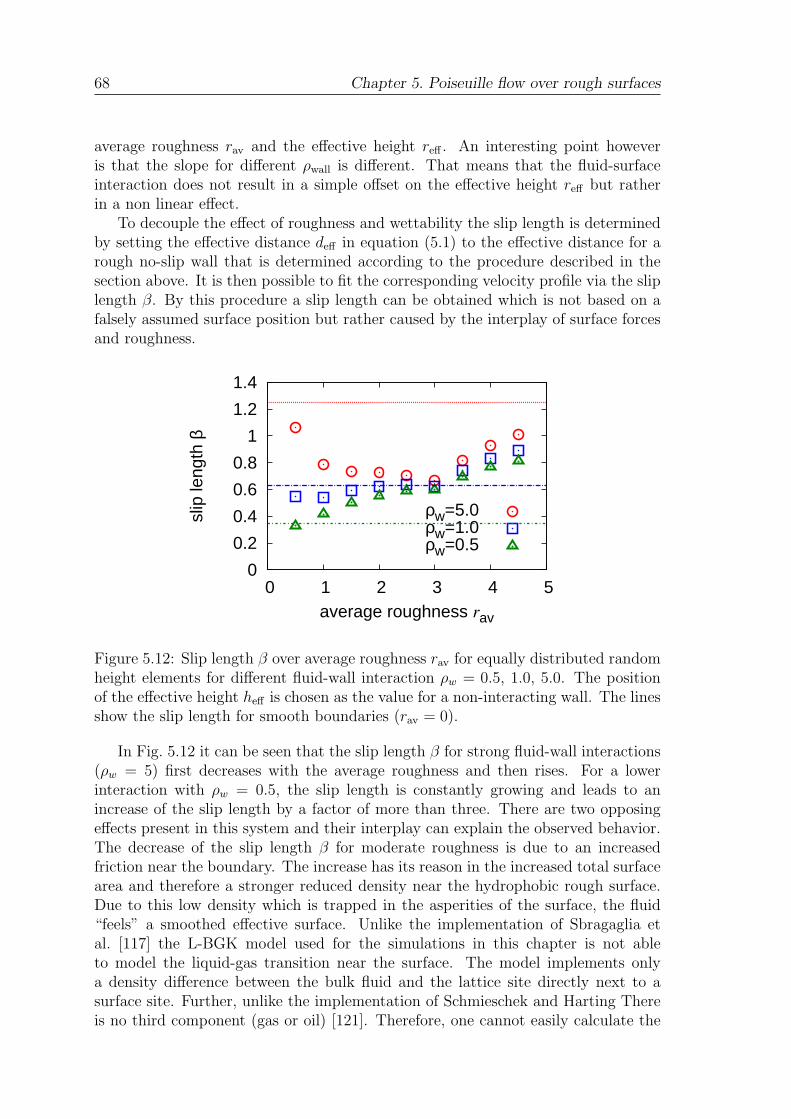
68 Chapter 5. Poiseuille flow over rough surfaces
average roughness rav and the effective height reff . An interesting point howeveris that the slope for different ρwall is different. That means that the fluid-surfaceinteraction does not result in a simple offset on the effective height reff but ratherin a non linear effect.
To decouple the effect of roughness and wettability the slip length is determinedby setting the effective distance deff in equation (5.1) to the effective distance for arough no-slip wall that is determined according to the procedure described in thesection above. It is then possible to fit the corresponding velocity profile via the sliplength β. By this procedure a slip length can be obtained which is not based on afalsely assumed surface position but rather caused by the interplay of surface forcesand roughness.
0
0.2
0.4
0.6
0.8
1
1.2
1.4
0 1 2 3 4 5
slip
leng
th β
average roughness rav
ρw=5.0ρw=1.0ρw=0.5
Figure 5.12: Slip length β over average roughness rav for equally distributed randomheight elements for different fluid-wall interaction ρw = 0.5, 1.0, 5.0. The positionof the effective height heff is chosen as the value for a non-interacting wall. The linesshow the slip length for smooth boundaries (rav = 0).
In Fig. 5.12 it can be seen that the slip length β for strong fluid-wall interactions(ρw = 5) first decreases with the average roughness and then rises. For a lowerinteraction with ρw = 0.5, the slip length is constantly growing and leads to anincrease of the slip length by a factor of more than three. There are two opposingeffects present in this system and their interplay can explain the observed behavior.The decrease of the slip length β for moderate roughness is due to an increasedfriction near the boundary. The increase has its reason in the increased total surfacearea and therefore a stronger reduced density near the hydrophobic rough surface.Due to this low density which is trapped in the asperities of the surface, the fluid“feels” a smoothed effective surface. Unlike the implementation of Sbragaglia etal. [117] the L-BGK model used for the simulations in this chapter is not ableto model the liquid-gas transition near the surface. The model implements onlya density difference between the bulk fluid and the lattice site directly next to asurface site. Further, unlike the implementation of Schmieschek and Harting Thereis no third component (gas or oil) [121]. Therefore, one cannot easily calculate the
5.3. Rough hydrophobic surfaces 69
contact angle in the presented simulations in contrast to the results presented byBenzi et al. [8]. This is due to the fact, that for a contact angle three phases (typicalgas, droplet and wall) are needed. However, the general effect of a pressure dropnear a hydrophobic surface is the same as in the model used by Sbragaglia [117].It can therefore be used to explain the behavior of polymer melts close to roughhydrophobic surfaces. In such a system the shorter polymer chains are enrichedclose to the boundary leading to a low viscous layer [6]. For a more detailed studyon super-hydrophobic surfaces, the strong surface variation as well as the liquid-gastransitions have to be taken into account.
Resume
In this chapter Poiseuille flow between two rough surfaces is studied. The conceptof an effective boundary position is introduced. Further, the effective boundaryposition for different surface geometries is investigated. A key result is that theeffective boundary position mainly depends on the maximum roughness height rand the distribution of the roughness height. The actual shape of the roughnesselements or the average roughness height have only a minor influence on the positionof the effective boundary. Furthermore, it was shown that the interplay of roughnessand surface wettability can lead to non-linear effects regarding the value of the sliplength.

70 Chapter 5. Poiseuille flow over rough surfaces
Chapter 6
Lubrication force on a sphereapproaching a flat surface
The main part of this work concentrates on the simulation of the AFM based slipexperiments. Therefore, it is necessary that the simulation method is tested welland the best simulation volume which is small enough to keep finite size effectsbelow an acceptable limit but still allows fast simulations is found. Further, it hasto be assured that the simulation method is able to reproduce the well establishedtheoretical solutions for cases where analytical solutions exist. One of them which isapplicable, is the theory of Brenner and Maude for the case of a sphere submergedin a Newtonian liquid that is approached towards a surface. In this chapter it willbe assured that this theory is reproduced by the simulation method and that finitesize effects can be avoided by choosing the correct boundary condition.
6.1 Discretization effects without boundaries
Finite size effects commonly occur in computer simulations because one has limitedresources, thus the simulated systems are small compared to experiments. There-fore, the boundaries of the system are much closer to the region of interest thanin experiments and in contrast to most theories which typically assume an infinitevolume. A typical approach to limit finite size effects is to use periodic boundaryconditions. However, in such a system the region of interest then interacts withits periodic images. Hasimoto gives a theoretical solution for the drag force of asphere in a periodic array as it appears in a simulation where all boundaries areperiodic [51]:
FHa =FSt
1 − 2.83a + 4.19a3 − 27.4a7 + O(a9)(6.1)
Here, a = R/n is the ratio between the radius of the sphere R and the system lengthn. The Stokes force is given by
FSt = 6πµRv, (6.2)
with µ being the viscosity of the liquid and v the velocity of the sphere.Besides a finite simulated volume most simulation methods utilize a finite dis-
cretization of the simulated objects, i.e., the sphere in our case consists of many
71
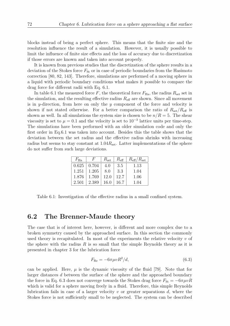
72 Chapter 6. Lubrication force on a sphere approaching a flat surface
blocks instead of being a perfect sphere. This means that the finite size and theresolution influence the result of a simulation. However, it is usually possible tolimit the influence of finite size effects and the loss of accuracy due to discretizationif those errors are known and taken into account properly.
It is known from previous studies that the discretization of the sphere results in adeviation of the Stokes force FSt or in case of periodic boundaries from the Hasimotocorrection [80, 82, 143]. Therefore, simulations are performed of a moving sphere ina liquid with periodic boundary conditions what makes it possible to compare thedrag force for different radii with Eq. 6.1.
In table 6.1 the measured force F , the theoretical force FHa, the radius Rset set inthe simulation, and the resulting effective radius Reff are shown. Since all movementis in y-direction, from here on only the y component of the force and velocity isshown if not stated otherwise. For a better comparison the ratio of Rset/Reff isshown as well. In all simulations the system size is chosen to be n/R = 5. The shearviscosity is set to µ = 0.1 and the velocity is set to 10−3 lattice units per time-step.The simulations have been performed with an older simulation code and only thefirst order in Eq.6.1 was taken into account. Besides this the table shows that thedeviation between the set radius and the effective radius shrinks with increasingradius but seems to stay constant at 1.04Rset. Latter implementations of the spheredo not suffer from such large deviations.
FHa F Rset Reff Reff/Rset
0.625 0.704 4.0 3.5 1.131.251 1.205 8.0 3.3 1.041.876 1.769 12.0 12.7 1.062.501 2.389 16.0 16.7 1.04
Table 6.1: Investigation of the effective radius in a small confined system.
6.2 The Brenner-Maude theory
The case that is of interest here, however, is different and more complex due to abroken symmetry caused by the approached surface. In this section the commonlyused theory is recapitulated. In most of the experiments the relative velocity v ofthe sphere with the radius R is so small that the simple Reynolds theory as it ispresented in chapter 3 for the lubrication force
FRe = −6πµvR2/d, (6.3)
can be applied. Here, µ is the dynamic viscosity of the fluid [79]. Note that forlarger distances d between the surface of the sphere and the approached boundarythe force in Eq. 6.3 does not converge towards the Stokes drag force FSt = −6πµvRwhich is valid for a sphere moving freely in a fluid. Therefore, this simple Reynoldslubrication fails in case of a larger velocity v or greater separations d, where theStokes force is not sufficiently small to be neglected. The system can be described
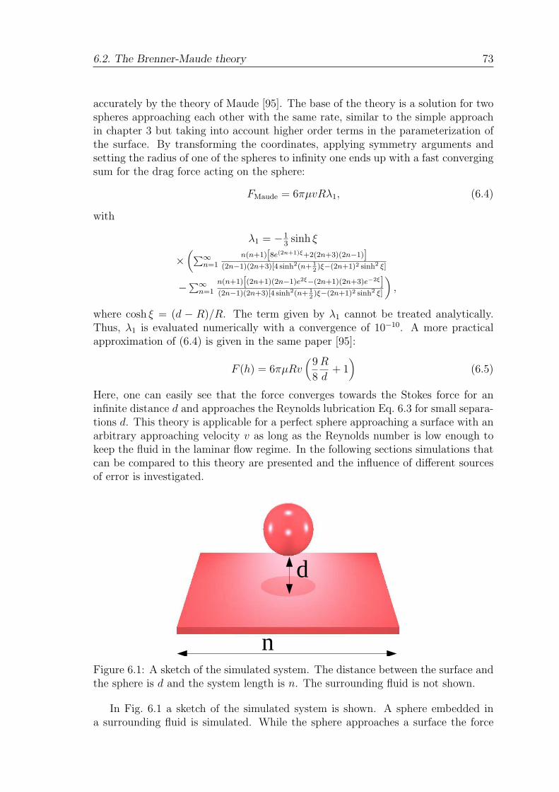
6.2. The Brenner-Maude theory 73
accurately by the theory of Maude [95]. The base of the theory is a solution for twospheres approaching each other with the same rate, similar to the simple approachin chapter 3 but taking into account higher order terms in the parameterization ofthe surface. By transforming the coordinates, applying symmetry arguments andsetting the radius of one of the spheres to infinity one ends up with a fast convergingsum for the drag force acting on the sphere:
FMaude = 6πµvRλ1, (6.4)
with
λ1 = −13sinh ξ
×(
∑∞n=1
n(n+1)[8e(2n+1)ξ+2(2n+3)(2n−1)](2n−1)(2n+3)[4 sinh2(n+ 1
2)ξ−(2n+1)2 sinh2 ξ]
−∑∞n=1
n(n+1)[(2n+1)(2n−1)e2ξ−(2n+1)(2n+3)e−2ξ](2n−1)(2n+3)[4 sinh2(n+ 1
2)ξ−(2n+1)2 sinh2 ξ]
)
,
where cosh ξ = (d − R)/R. The term given by λ1 cannot be treated analytically.Thus, λ1 is evaluated numerically with a convergence of 10−10. A more practicalapproximation of (6.4) is given in the same paper [95]:
F (h) = 6πµRv(
9
8
R
d+ 1
)
(6.5)
Here, one can easily see that the force converges towards the Stokes force for aninfinite distance d and approaches the Reynolds lubrication Eq. 6.3 for small separa-tions d. This theory is applicable for a perfect sphere approaching a surface with anarbitrary approaching velocity v as long as the Reynolds number is low enough tokeep the fluid in the laminar flow regime. In the following sections simulations thatcan be compared to this theory are presented and the influence of different sourcesof error is investigated.
d
nFigure 6.1: A sketch of the simulated system. The distance between the surface andthe sphere is d and the system length is n. The surrounding fluid is not shown.
In Fig. 6.1 a sketch of the simulated system is shown. A sphere embedded ina surrounding fluid is simulated. While the sphere approaches a surface the force

74 Chapter 6. Lubrication force on a sphere approaching a flat surface
acting on it is recorded. Due to the jump-like movement of the sphere the force showsa significant noise from time-step to time-step which makes it necessary to averagethe force and to keep the velocity low so that the fluid can relax after a reformation ofthe boundary nodes. Simulations with different sphere radii R and different systemwidth n are performed to investigate finite size effects. For simplicity the x and zdimensions are set to the same value n and the propagation dimension y is keptconstant at 512 lattice units. If not stated otherwise the simulation parameters arev = 0.001, µ = 0.1, and the radius is varied between R = 4 and R = 16. The typicalforce averaging is done over 333 time-steps. It is assured that the averaging doesnot influence the results, i.e. the results for averaging over 99 up to 999 time stepsare compared and no significant deviation is found. 333 time steps reduce the noisestrongly while the spatial coarse -graining due to the constant velocity is over 0.3lattice sites which is a good spatial resolution. For a better visibility of the datapoints only a fraction of them is plotted. The approached boundary is a plain no-slipwall which is realized by a mid-grid bounce back boundary condition. Along theopen sides periodic boundary conditions are applied so that the sphere can interactwith its mirror images leading to undesired finite size effects.
6.3 Finite size effects with boundaries
A major contribution to the finite size effects is the interaction of the sphere withits periodic image. Therefore, a larger system length should reduce this effect dra-matically. However, when the hydrodynamic influence of the wall becomes larger,finite size effects become smaller. This can be explained by the fact that the frictionat the boundary suppresses the hydrodynamic interaction of the particle with itsperiodic image. Instead, the dominant interaction is between the particle and thesurface. It is mandatory for a better understanding of the system to learn how thesefinite size effects can be described, quantified, and controlled.
6.3.1 Large test
First, a run of a large 5123 system assures that the method really shows the desiredasymptotic behavior, i.e., it is able to reproduce the theory Maude. Further it hasto be checked that the force scales with the velocity. To demonstrate this behaviora long run with a smaller R = 8 sphere in a 2563 system is performed as well butwith a velocity of v = 10−4 instead of the usual 10−3 lattice nodes per time-step.Since the sphere is smaller by a factor of 2 it consumes a factor of 16 less computerpower to run a simulation in which all lengths are scaled by the radius. A factor of8 in the computer power is due to the smaller simulation volume and an additionalfactor of 2 due to the shorter length the sphere has to travel at the constant speedto travel the same fraction of its radius i.e. twice as many time steps have to beperformed. That is why the velocity independence is shown with R = 8. In additionintermediate velocities 10−4 < v < 10−3 are tested to assure the results but are notshown here for a better visibility of the main results.
The simulated data are plotted together with the first order approximation andthe theoretical values by Maude in Fig. 6.2. If not stated otherwise values in this
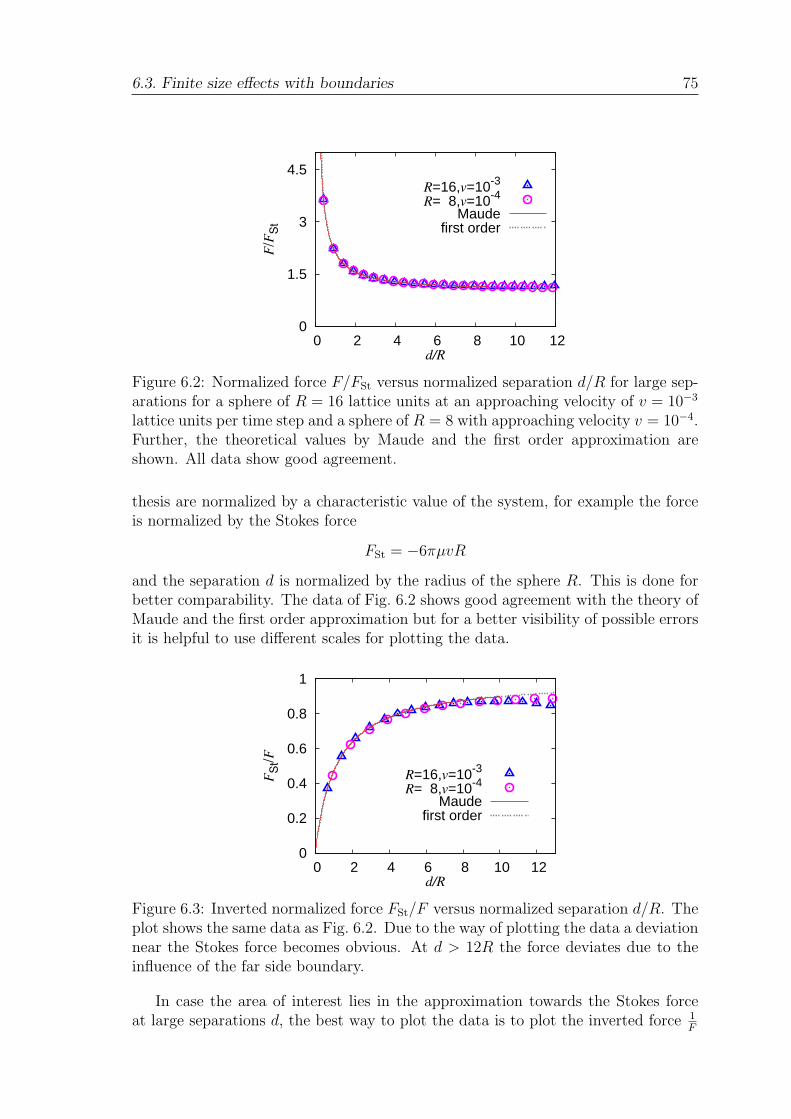
6.3. Finite size effects with boundaries 75
0
1.5
3
4.5
0 2 4 6 8 10 12
F/F
St
d/R
R=16,v=10-3
R= 8,v=10-4
Maudefirst order
Figure 6.2: Normalized force F/FSt versus normalized separation d/R for large sep-arations for a sphere of R = 16 lattice units at an approaching velocity of v = 10−3
lattice units per time step and a sphere of R = 8 with approaching velocity v = 10−4.Further, the theoretical values by Maude and the first order approximation areshown. All data show good agreement.
thesis are normalized by a characteristic value of the system, for example the forceis normalized by the Stokes force
FSt = −6πµvR
and the separation d is normalized by the radius of the sphere R. This is done forbetter comparability. The data of Fig. 6.2 shows good agreement with the theory ofMaude and the first order approximation but for a better visibility of possible errorsit is helpful to use different scales for plotting the data.
0
0.2
0.4
0.6
0.8
1
0 2 4 6 8 10 12
FS
t/F
d/R
R=16,v=10-3
R= 8,v=10-4
Maudefirst order
Figure 6.3: Inverted normalized force FSt/F versus normalized separation d/R. Theplot shows the same data as Fig. 6.2. Due to the way of plotting the data a deviationnear the Stokes force becomes obvious. At d > 12R the force deviates due to theinfluence of the far side boundary.
In case the area of interest lies in the approximation towards the Stokes forceat large separations d, the best way to plot the data is to plot the inverted force 1
F
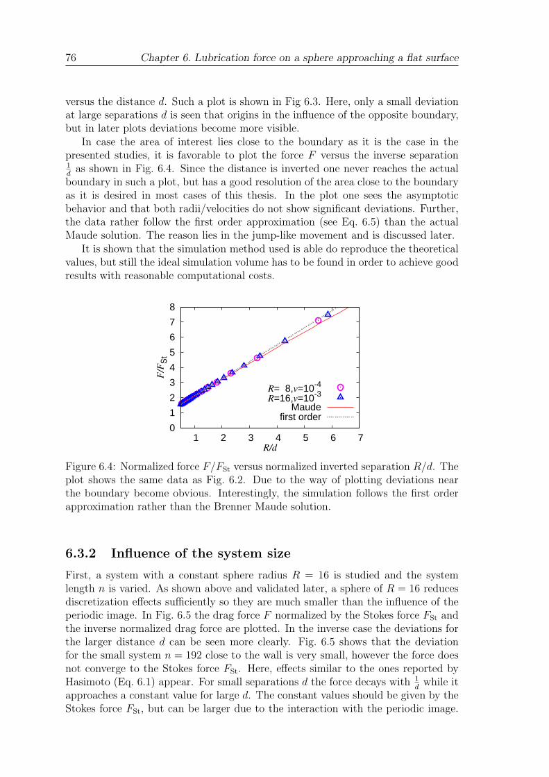
76 Chapter 6. Lubrication force on a sphere approaching a flat surface
versus the distance d. Such a plot is shown in Fig 6.3. Here, only a small deviationat large separations d is seen that origins in the influence of the opposite boundary,but in later plots deviations become more visible.
In case the area of interest lies close to the boundary as it is the case in thepresented studies, it is favorable to plot the force F versus the inverse separation1d
as shown in Fig. 6.4. Since the distance is inverted one never reaches the actualboundary in such a plot, but has a good resolution of the area close to the boundaryas it is desired in most cases of this thesis. In the plot one sees the asymptoticbehavior and that both radii/velocities do not show significant deviations. Further,the data rather follow the first order approximation (see Eq. 6.5) than the actualMaude solution. The reason lies in the jump-like movement and is discussed later.
It is shown that the simulation method used is able do reproduce the theoreticalvalues, but still the ideal simulation volume has to be found in order to achieve goodresults with reasonable computational costs.
0
1
2
3
4
5
6
7
8
1 2 3 4 5 6 7
F/F
St
R/d
R= 8,v=10-4
R=16,v=10-3
Maudefirst order
Figure 6.4: Normalized force F/FSt versus normalized inverted separation R/d. Theplot shows the same data as Fig. 6.2. Due to the way of plotting deviations nearthe boundary become obvious. Interestingly, the simulation follows the first orderapproximation rather than the Brenner Maude solution.
6.3.2 Influence of the system size
First, a system with a constant sphere radius R = 16 is studied and the systemlength n is varied. As shown above and validated later, a sphere of R = 16 reducesdiscretization effects sufficiently so they are much smaller than the influence of theperiodic image. In Fig. 6.5 the drag force F normalized by the Stokes force FSt andthe inverse normalized drag force are plotted. In the inverse case the deviations forthe larger distance d can be seen more clearly. Fig. 6.5 shows that the deviationfor the small system n = 192 close to the wall is very small, however the force doesnot converge to the Stokes force FSt. Here, effects similar to the ones reported byHasimoto (Eq. 6.1) appear. For small separations d the force decays with 1
dwhile it
approaches a constant value for large d. The constant values should be given by theStokes force FSt, but can be larger due to the interaction with the periodic image.
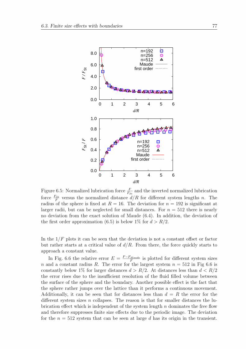
6.3. Finite size effects with boundaries 77
0.0
2.0
4.0
6.0
8.0
0 1 2 3 4 5 6
F /
FS
t
d/R
n=192n=256n=512Maude
first order
0.0
0.2
0.4
0.6
0.8
1.0
0 1 2 3 4 5 6
FS
t / F
d/R
n=192n=256n=512Maude
first order
Figure 6.5: Normalized lubrication force FFSt
and the inverted normalized lubrication
force FSt
Fversus the normalized distance d/R for different system lengths n. The
radius of the sphere is fixed at R = 16. The deviation for n = 192 is significant atlarger radii, but can be neglected for small distances. For n = 512 there is nearlyno deviation from the exact solution of Maude (6.4). In addition, the deviation ofthe first order approximation (6.5) is below 1% for d > R/2.
In the 1/F plots it can be seen that the deviation is not a constant offset or factorbut rather starts at a critical value of d/R. From there, the force quickly starts toapproach a constant value.
In Fig. 6.6 the relative error E = F−FMaude
Fis plotted for different system sizes
n and a constant radius R. The error for the largest system n = 512 in Fig 6.6 isconstantly below 1% for larger distances d > R/2. At distances less than d < R/2the error rises due to the insufficient resolution of the fluid filled volume betweenthe surface of the sphere and the boundary. Another possible effect is the fact thatthe sphere rather jumps over the lattice than it performs a continuous movement.Additionally, it can be seen that for distances less than d = R the error for thedifferent system sizes n collapses. The reason is that for smaller distances the lu-brication effect which is independent of the system length n dominates the free flowand therefore suppresses finite size effects due to the periodic image. The deviationfor the n = 512 system that can be seen at large d has its origin in the transient.
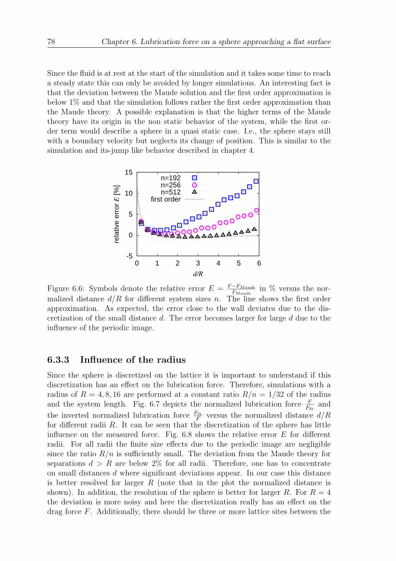
78 Chapter 6. Lubrication force on a sphere approaching a flat surface
Since the fluid is at rest at the start of the simulation and it takes some time to reacha steady state this can only be avoided by longer simulations. An interesting fact isthat the deviation between the Maude solution and the first order approximation isbelow 1% and that the simulation follows rather the first order approximation thanthe Maude theory. A possible explanation is that the higher terms of the Maudetheory have its origin in the non static behavior of the system, while the first or-der term would describe a sphere in a quasi static case. I.e., the sphere stays stillwith a boundary velocity but neglects its change of position. This is similar to thesimulation and its-jump like behavior described in chapter 4.
-5
0
5
10
15
0 1 2 3 4 5 6
rela
tive
erro
r E
[%]
d/R
n=192n=256n=512
first order
Figure 6.6: Symbols denote the relative error E = F−FMaude
FMaudein % versus the nor-
malized distance d/R for different system sizes n. The line shows the first orderapproximation. As expected, the error close to the wall deviates due to the dis-cretization of the small distance d. The error becomes larger for large d due to theinfluence of the periodic image.
6.3.3 Influence of the radius
Since the sphere is discretized on the lattice it is important to understand if thisdiscretization has an effect on the lubrication force. Therefore, simulations with aradius of R = 4, 8, 16 are performed at a constant ratio R/n = 1/32 of the radiusand the system length. Fig. 6.7 depicts the normalized lubrication force F
FStand
the inverted normalized lubrication force FSt
Fversus the normalized distance d/R
for different radii R. It can be seen that the discretization of the sphere has littleinfluence on the measured force. Fig. 6.8 shows the relative error E for differentradii. For all radii the finite size effects due to the periodic image are negligiblesince the ratio R/n is sufficiently small. The deviation from the Maude theory forseparations d > R are below 2% for all radii. Therefore, one has to concentrateon small distances d where significant deviations appear. In our case this distanceis better resolved for larger R (note that in the plot the normalized distance isshown). In addition, the resolution of the sphere is better for larger R. For R = 4the deviation is more noisy and here the discretization really has an effect on thedrag force F . Additionally, there should be three or more lattice sites between the
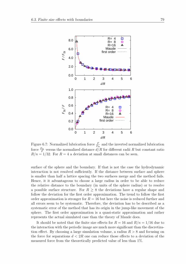
6.3. Finite size effects with boundaries 79
0.0
2.0
4.0
6.0
8.0
0 1 2 3 4 5 6
F /
FS
t
d/R
R= 4R= 8R=16
Maudefirst order
0.0
0.2
0.4
0.6
0.8
1.0
0 1 2 3 4 5 6
FS
t / F
d/R
R= 4R= 8R=16
Maudefirst order
Figure 6.7: Normalized lubrication force FFSt
and the inverted normalized lubrication
force FSt
Fversus the normalized distance d/R for different radii R but constant ratio
R/n = 1/32. For R = 4 a deviation at small distances can be seen.
surface of the sphere and the boundary. If that is not the case the hydrodynamicinteraction is not resolved sufficiently. If the distance between surface and sphereis smaller than half a lattice spacing the two surfaces merge and the method fails.Hence, it it advantageous to choose a large radius in order to be able to reducethe relative distance to the boundary (in units of the sphere radius) or to resolvea possible surface structure. For R ≥ 8 the deviations have a regular shape andfollow the deviation for the first order approximation. The trend to follow the firstorder approximation is stronger for R = 16 but here the noise is reduced further andall errors seem to be systematic. Therefore, the deviation has to be described as asystematic error of the method that has its origin in the jump-like movement of thesphere. The first order approximation is a quasi-static approximation and ratherrepresents the actual simulated case than the theory of Maude does.
It should be noted that the finite size effects for R = 16 and R/n = 1/16 due tothe interaction with the periodic image are much more significant than the discretiza-tion effect. By choosing a large simulation volume, a radius R > 8 and focusing onthe force for separations d < 2R one can reduce those effects to a deviation of themeasured force from the theoretically predicted value of less than 1%.
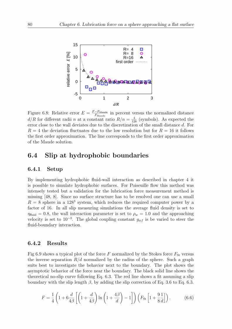
80 Chapter 6. Lubrication force on a sphere approaching a flat surface
-5
0
5
10
15
0 1 2 3
rela
tive
erro
r E
[%]
d/R
R= 4R= 8R=16
first order
Figure 6.8: Relative error E = F−FMaude
FMaudein percent versus the normalized distance
d/R for different radii n at a constant ratio R/n = 4128
(symbols). As expected theerror close to the wall deviates due to the discretization of the small distance d. ForR = 4 the deviation fluctuates due to the low resolution but for R = 16 it followsthe first order approximation. The line corresponds to the first order approximationof the Maude solution.
6.4 Slip at hydrophobic boundaries
6.4.1 Setup
By implementing hydrophobic fluid-wall interaction as described in chapter 4 itis possible to simulate hydrophobic surfaces. For Poiseuille flow this method wasintensely tested but a validation for the lubrication force measurement method ismissing [48, 8]. Since no surface structure has to be resolved one can use a smallR = 8 sphere in a 1283 system, which reduces the required computer power by afactor of 16. In all slip measuring simulations the average fluid density is set toηfluid = 0.8, the wall interaction parameter is set to ρw = 1.0 and the approachingvelocity is set to 10−3. The global coupling constant gwf is be varied to steer thefluid-boundary interaction.
6.4.2 Results
Fig 6.9 shows a typical plot of the force F normalized by the Stokes force FSt versusthe inverse separation R/d normalized by the radius of the sphere. Such a graphsuits best to investigate the behavior next to the boundary. The plot shows theasymptotic behavior of the force near the boundary. The black solid line shows thetheoretical no-slip curve following Eq. 6.3. The red line shows a fit assuming a slipboundary with the slip length β, by adding the slip correction of Eq. 3.6 to Eq. 6.3.
F =1
4
(
1 + 6d
4β
[(
1 +d
4β
)
ln
(
1 +4β
d
)
− 1
])
(
FSt
[
1 +9
8
1
d
])
. (6.6)
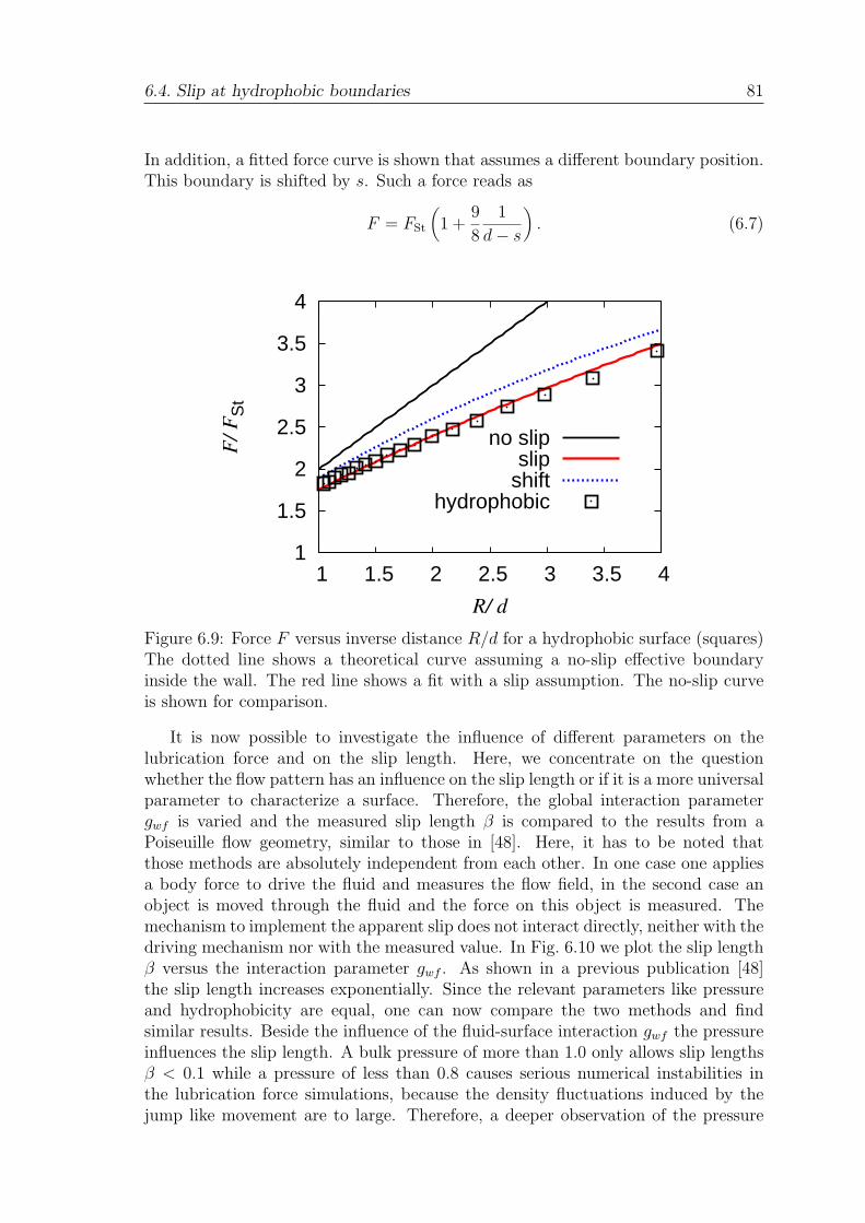
6.4. Slip at hydrophobic boundaries 81
In addition, a fitted force curve is shown that assumes a different boundary position.This boundary is shifted by s. Such a force reads as
F = FSt
(
1 +9
8
1
d − s
)
. (6.7)
1
1.5
2
2.5
3
3.5
4
1 1.5 2 2.5 3 3.5 4
F/
FS
t
R/ d
no slipslip
shifthydrophobic
Figure 6.9: Force F versus inverse distance R/d for a hydrophobic surface (squares)The dotted line shows a theoretical curve assuming a no-slip effective boundaryinside the wall. The red line shows a fit with a slip assumption. The no-slip curveis shown for comparison.
It is now possible to investigate the influence of different parameters on thelubrication force and on the slip length. Here, we concentrate on the questionwhether the flow pattern has an influence on the slip length or if it is a more universalparameter to characterize a surface. Therefore, the global interaction parametergwf is varied and the measured slip length β is compared to the results from aPoiseuille flow geometry, similar to those in [48]. Here, it has to be noted thatthose methods are absolutely independent from each other. In one case one appliesa body force to drive the fluid and measures the flow field, in the second case anobject is moved through the fluid and the force on this object is measured. Themechanism to implement the apparent slip does not interact directly, neither with thedriving mechanism nor with the measured value. In Fig. 6.10 we plot the slip lengthβ versus the interaction parameter gwf . As shown in a previous publication [48]the slip length increases exponentially. Since the relevant parameters like pressureand hydrophobicity are equal, one can now compare the two methods and findsimilar results. Beside the influence of the fluid-surface interaction gwf the pressureinfluences the slip length. A bulk pressure of more than 1.0 only allows slip lengthsβ < 0.1 while a pressure of less than 0.8 causes serious numerical instabilities inthe lubrication force simulations, because the density fluctuations induced by thejump like movement are to large. Therefore, a deeper observation of the pressure
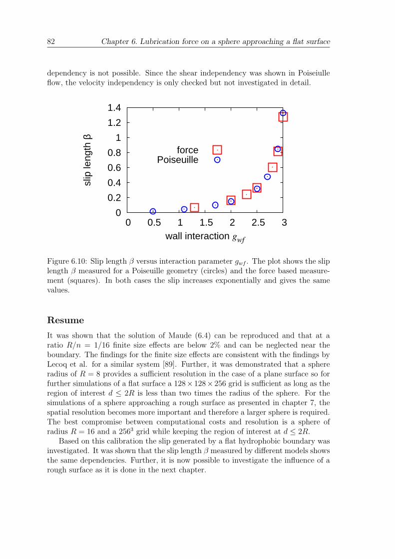
82 Chapter 6. Lubrication force on a sphere approaching a flat surface
dependency is not possible. Since the shear independency was shown in Poiseiulleflow, the velocity independency is only checked but not investigated in detail.
0
0.2
0.4
0.6
0.8
1
1.2
1.4
0 0.5 1 1.5 2 2.5 3
slip
leng
th β
wall interaction gwf
forcePoiseuille
Figure 6.10: Slip length β versus interaction parameter gwf . The plot shows the sliplength β measured for a Poiseuille geometry (circles) and the force based measure-ment (squares). In both cases the slip increases exponentially and gives the samevalues.
Resume
It was shown that the solution of Maude (6.4) can be reproduced and that at aratio R/n = 1/16 finite size effects are below 2% and can be neglected near theboundary. The findings for the finite size effects are consistent with the findings byLecoq et al. for a similar system [89]. Further, it was demonstrated that a sphereradius of R = 8 provides a sufficient resolution in the case of a plane surface so forfurther simulations of a flat surface a 128× 128× 256 grid is sufficient as long as theregion of interest d ≤ 2R is less than two times the radius of the sphere. For thesimulations of a sphere approaching a rough surface as presented in chapter 7, thespatial resolution becomes more important and therefore a larger sphere is required.The best compromise between computational costs and resolution is a sphere ofradius R = 16 and a 2563 grid while keeping the region of interest at d ≤ 2R.
Based on this calibration the slip generated by a flat hydrophobic boundary wasinvestigated. It was shown that the slip length β measured by different models showsthe same dependencies. Further, it is now possible to investigate the influence of arough surface as it is done in the next chapter.

Chapter 7
Lubrication force on a sphereapproaching a rough surface
After the presentation of simulations of a flat surface in the previous chapter whichshowed that the common theories for Lubrication flow can be reproduced, simula-tions of a sphere approaching a rough surface are presented in this chapter. Sincereal surfaces are never perfectly smooth this work has an influence on the interpre-tation of slip experiments. In tis chapter it are shown that the lubrication force ona sphere approaching a rough boundary cannot be described by a slip correction f ∗
Eq: 3.6 but by a shift of the effective boundary in a manner similar to chapter 5.
7.1 Setup
point of contact
r
h
yz
x
h
contact
r
point of
Figure 7.1: Sketch of the system: a sphere with radius R approaches a rough surfacewhere a fixed area fraction φ is covered by roughness elements. The separation h isdefined on top of the surface roughness at position y = r.
Computer simulations provide the opportunity to vary different parameters and
83
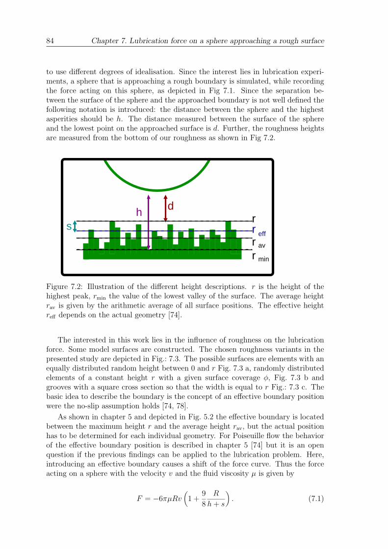
84 Chapter 7. Lubrication force on a sphere approaching a rough surface
to use different degrees of idealisation. Since the interest lies in lubrication experi-ments, a sphere that is approaching a rough boundary is simulated, while recordingthe force acting on this sphere, as depicted in Fig 7.1. Since the separation be-tween the surface of the sphere and the approached boundary is not well defined thefollowing notation is introduced: the distance between the sphere and the highestasperities should be h. The distance measured between the surface of the sphereand the lowest point on the approached surface is d. Further, the roughness heightsare measured from the bottom of our roughness as shown in Fig 7.2.
av
min
eff
rrrr
dhs
Figure 7.2: Illustration of the different height descriptions. r is the height of thehighest peak, rmin the value of the lowest valley of the surface. The average heightrav is given by the arithmetic average of all surface positions. The effective heightreff depends on the actual geometry [74].
The interested in this work lies in the influence of roughness on the lubricationforce. Some model surfaces are constructed. The chosen roughness variants in thepresented study are depicted in Fig.: 7.3. The possible surfaces are elements with anequally distributed random height between 0 and r Fig. 7.3 a, randomly distributedelements of a constant height r with a given surface coverage φ, Fig. 7.3 b andgrooves with a square cross section so that the width is equal to r Fig.: 7.3 c. Thebasic idea to describe the boundary is the concept of an effective boundary positionwere the no-slip assumption holds [74, 78].
As shown in chapter 5 and depicted in Fig. 5.2 the effective boundary is locatedbetween the maximum height r and the average height rav, but the actual positionhas to be determined for each individual geometry. For Poiseuille flow the behaviorof the effective boundary position is described in chapter 5 [74] but it is an openquestion if the previous findings can be applied to the lubrication problem. Here,introducing an effective boundary causes a shift of the force curve. Thus the forceacting on a sphere with the velocity v and the fluid viscosity µ is given by
F = −6πµRv(
1 +9
8
R
h + s
)
. (7.1)
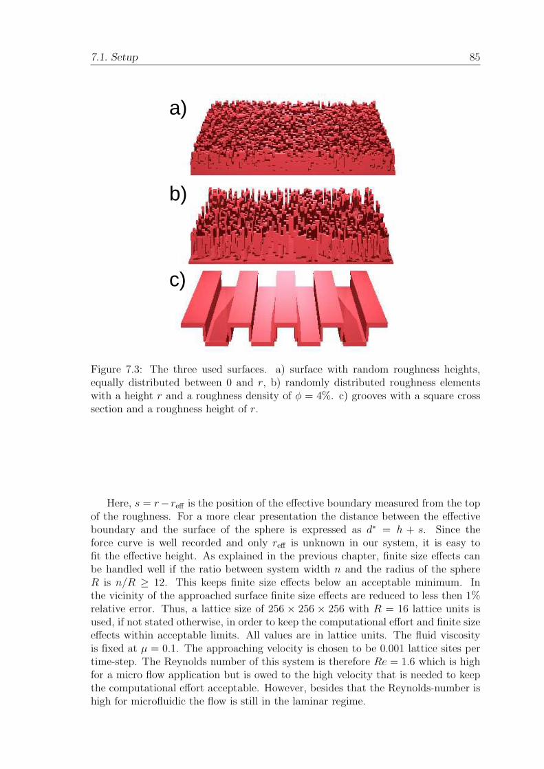
7.1. Setup 85
c)
b)
a)
Figure 7.3: The three used surfaces. a) surface with random roughness heights,equally distributed between 0 and r, b) randomly distributed roughness elementswith a height r and a roughness density of φ = 4%. c) grooves with a square crosssection and a roughness height of r.
Here, s = r− reff is the position of the effective boundary measured from the topof the roughness. For a more clear presentation the distance between the effectiveboundary and the surface of the sphere is expressed as d∗ = h + s. Since theforce curve is well recorded and only reff is unknown in our system, it is easy tofit the effective height. As explained in the previous chapter, finite size effects canbe handled well if the ratio between system width n and the radius of the sphereR is n/R ≥ 12. This keeps finite size effects below an acceptable minimum. Inthe vicinity of the approached surface finite size effects are reduced to less then 1%relative error. Thus, a lattice size of 256 × 256 × 256 with R = 16 lattice units isused, if not stated otherwise, in order to keep the computational effort and finite sizeeffects within acceptable limits. All values are in lattice units. The fluid viscosityis fixed at µ = 0.1. The approaching velocity is chosen to be 0.001 lattice sites pertime-step. The Reynolds number of this system is therefore Re = 1.6 which is highfor a micro flow application but is owed to the high velocity that is needed to keepthe computational effort acceptable. However, besides that the Reynolds-number ishigh for microfluidic the flow is still in the laminar regime.

86 Chapter 7. Lubrication force on a sphere approaching a rough surface
0
0.2
0.4
0.6
0 0.5 1 1.5 2
FS
t/F
h/R
flatslip β=2.43
reff=7.86φ= 4%φ=50%
0
1
2
3
4
5
1 2 3 4 5 6 7 8
F/F
St
R/h
flatslip β=2.43
reff=7.86φ= 4%φ=50%
Figure 7.4: Drag force F versus separation h plotted in different coordinates. Onthe left hand side the inverse force FSt/F versus the normalised separation h/R andon the right the normalised force F/FSt versus the inverse distance R/h is plotted.They show the measured force for two rough surfaces with r = 11, φ = 4% andφ = 50%. For φ = 4% the asymptotic behavior for small h cannot be fitted witha slip, but the assumption of an effective boundary position holds. The values forφ = 50% nearly recover the case of a flat surface at r. For comparison a fit with aslip theory a boundary shift and a flat surface at the top of the asperities is plottedas well.
7.2 Results
First the effect of roughness is compared with the effect of apparent slip as presentedin the previous chapter and it is shown that the assumption of an effective boundaryposition can be distinguished from a slip surface assumption. Then, it is investigatedto what extend the effective boundary assumption holds and whether it differs fromthe previous results in a Poiseuille flow geometry,
7.3 Comparison of roughness and slip
The focus of this section is on drag force measurements near surfaces with randomlydistributed roughness elements as shown in Fig. 7.3 b, where the chosen roughnessis characterized by the two parameters r and φ. Such a roughness mimic someexperiment ally used surfaces, like those utilizing a carbon-nano-tube forest [66].Further, one is able to generate a well controlled surface with only two parameters,namely the roughness density φ and the roughness height r. Since it was shown inchapter 6 that for a hydrophobic surface the theoretical expectations (like Eq. 3.6) are fulfilled simulations of a sphere that approaches a rough surface are presentednow.
In Fig. 7.4 left the inverse normalized lubrication force FSt/F versus the nor-malized separation h/R is shown for surfaces with φ = 4%, φ = 50%, and r = 11,while in Fig. 7.4 right the normalized hydrodynamic resistance force F/FSt versusthe inverse separation R/h is plotted. Also shown in both plots are the theory for a
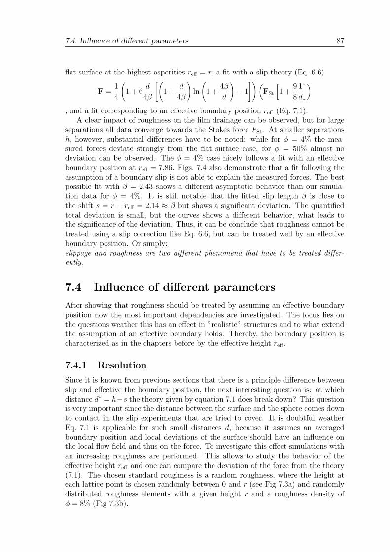
7.4. Influence of different parameters 87
flat surface at the highest asperities reff = r, a fit with a slip theory (Eq. 6.6)
F =1
4
(
1 + 6d
4β
[(
1 +d
4β
)
ln
(
1 +4β
d
)
− 1
])
(
FSt
[
1 +9
8
1
d
])
, and a fit corresponding to an effective boundary position reff (Eq. 7.1).A clear impact of roughness on the film drainage can be observed, but for large
separations all data converge towards the Stokes force FSt. At smaller separationsh, however, substantial differences have to be noted: while for φ = 4% the mea-sured forces deviate strongly from the flat surface case, for φ = 50% almost nodeviation can be observed. The φ = 4% case nicely follows a fit with an effectiveboundary position at reff = 7.86. Figs. 7.4 also demonstrate that a fit following theassumption of a boundary slip is not able to explain the measured forces. The bestpossible fit with β = 2.43 shows a different asymptotic behavior than our simula-tion data for φ = 4%. It is still notable that the fitted slip length β is close tothe shift s = r − reff = 2.14 ≈ β but shows a significant deviation. The quantifiedtotal deviation is small, but the curves shows a different behavior, what leads tothe significance of the deviation. Thus, it can be conclude that roughness cannot betreated using a slip correction like Eq. 6.6, but can be treated well by an effectiveboundary position. Or simply:slippage and roughness are two different phenomena that have to be treated differ-ently.
7.4 Influence of different parameters
After showing that roughness should be treated by assuming an effective boundaryposition now the most important dependencies are investigated. The focus lies onthe questions weather this has an effect in ”realistic” structures and to what extendthe assumption of an effective boundary holds. Thereby, the boundary position ischaracterized as in the chapters before by the effective height reff .
7.4.1 Resolution
Since it is known from previous sections that there is a principle difference betweenslip and effective the boundary position, the next interesting question is: at whichdistance d∗ = h−s the theory given by equation 7.1 does break down? This questionis very important since the distance between the surface and the sphere comes downto contact in the slip experiments that are tried to cover. It is doubtful weatherEq. 7.1 is applicable for such small distances d, because it assumes an averagedboundary position and local deviations of the surface should have an influence onthe local flow field and thus on the force. To investigate this effect simulations withan increasing roughness are performed. This allows to study the behavior of theeffective height reff and one can compare the deviation of the force from the theory(7.1). The chosen standard roughness is a random roughness, where the height ateach lattice point is chosen randomly between 0 and r (see Fig 7.3a) and randomlydistributed roughness elements with a given height r and a roughness density ofφ = 8% (Fig 7.3b).

88 Chapter 7. Lubrication force on a sphere approaching a rough surface
0
2
4
6
8
10
0 0.5 1 1.5 2
F/F
St
d*/R
r = 2r = 6r =10r =14
Theory
0
2
4
6
8
10
0 0.5 1 1.5 2
F/F
St
d*/R
r = 2r = 6r =10r =14
Theory
Figure 7.5: Lubrication force F normalized by FSt versus the normalized distanced∗/R between the surface of the sphere and the effective boundary for differentmaximum heights r in a system with random heights (left) and randomly distributedroughness elements φ = 8% (right) for different maximum heights r. The theory isgiven by Eq. 7.1. A deviation of the force from the theory is not found up to d < 3lattice sites. Below this discretization is to strong to give quantitative results.
In Fig. 7.5 the lubrication force F/FSt versus the normalized distance d∗/R be-tween the effective height and the surface of the sphere is shown for different rough-ness heights. The lubrication force F is normalized by the Stokes force FSt. Thetheoretical curve for a plain surface is plotted as well. The force increases rapidlyfor small distances and converges slowly towards the Stokes force FSt for longer dis-tances. This convergence is not shown in the plot since only short distances wherethe surface-fluid interaction has its main influence, are plotted. The deviation fromthe theory (7.1) is below 2% at a distance less then d∗ > 3 lattice sites. Here, it hasto be noted that a minimum distance of three lattice nodes is needed to resolve thefluid flow correctly. The error for smaller distances than d < 2 lattice sites becomeslarge but since the fluid field away from the point of contact is resolved sufficientlythe strong increase of the force for < 2 lattice sites is still covered by the simulation.
Similar to previous plots the deviations are more obvious in a force versus theinverted distance plot as shown in Fig. 7.6. This can be seen at the error for a flatboundary r = 0 in Fig. 7.7. However the astonishing result is that the deviationstarts very close to the boundary, so the concept of an effective boundary can beapplied for small distances as well.
For a better illustration of the error, the relative deviation δF between the theory(7.1) and the simulation data, is plotted over the effective distance d∗ in Fig. 7.7.Note that in this case the distance is given in lattice units and is not normalizedby the radius. This is done in order to distinguish weather the deviation origins ina discretization effect or if the physical background does not hold in this case. Byplotting the distance in lattice units one can see how strongly the space between thesurfaces is discretized. Further it is known from the previous chapter what is theeffect of the discretization.
For both kinds of roughness the plots are similar. For the moderate roughnessesof r < 10 the relative error of the measured force F towards equation 7.1 is below2% down to a distance of d∗ > 5x. At smaller distances the error starts to increase
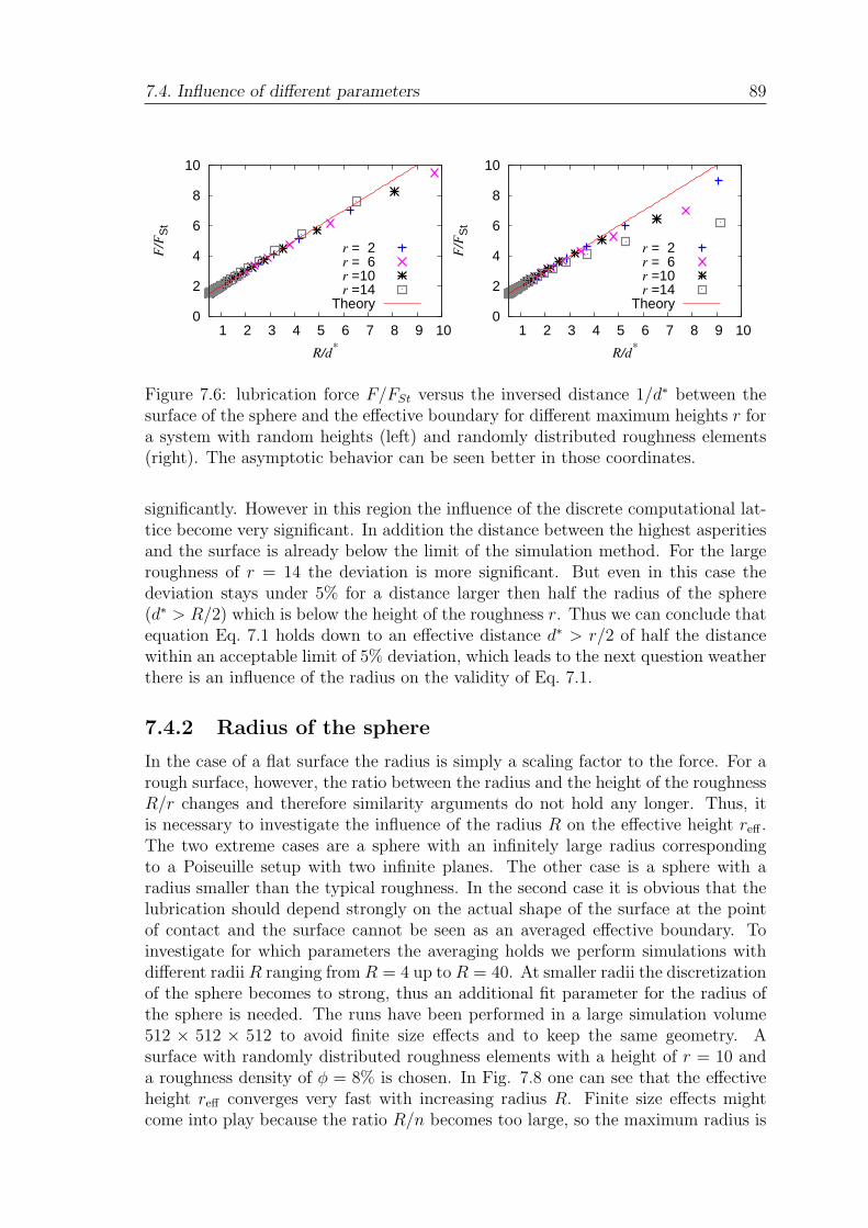
7.4. Influence of different parameters 89
0
2
4
6
8
10
1 2 3 4 5 6 7 8 9 10
F/F
St
R/d*
r = 2r = 6r =10r =14
Theory 0
2
4
6
8
10
1 2 3 4 5 6 7 8 9 10
F/F
St
R/d*
r = 2r = 6r =10r =14
Theory
Figure 7.6: lubrication force F/FSt versus the inversed distance 1/d∗ between thesurface of the sphere and the effective boundary for different maximum heights r fora system with random heights (left) and randomly distributed roughness elements(right). The asymptotic behavior can be seen better in those coordinates.
significantly. However in this region the influence of the discrete computational lat-tice become very significant. In addition the distance between the highest asperitiesand the surface is already below the limit of the simulation method. For the largeroughness of r = 14 the deviation is more significant. But even in this case thedeviation stays under 5% for a distance larger then half the radius of the sphere(d∗ > R/2) which is below the height of the roughness r. Thus we can conclude thatequation Eq. 7.1 holds down to an effective distance d∗ > r/2 of half the distancewithin an acceptable limit of 5% deviation, which leads to the next question weatherthere is an influence of the radius on the validity of Eq. 7.1.
7.4.2 Radius of the sphere
In the case of a flat surface the radius is simply a scaling factor to the force. For arough surface, however, the ratio between the radius and the height of the roughnessR/r changes and therefore similarity arguments do not hold any longer. Thus, itis necessary to investigate the influence of the radius R on the effective height reff .The two extreme cases are a sphere with an infinitely large radius correspondingto a Poiseuille setup with two infinite planes. The other case is a sphere with aradius smaller than the typical roughness. In the second case it is obvious that thelubrication should depend strongly on the actual shape of the surface at the pointof contact and the surface cannot be seen as an averaged effective boundary. Toinvestigate for which parameters the averaging holds we perform simulations withdifferent radii R ranging from R = 4 up to R = 40. At smaller radii the discretizationof the sphere becomes to strong, thus an additional fit parameter for the radius ofthe sphere is needed. The runs have been performed in a large simulation volume512 × 512 × 512 to avoid finite size effects and to keep the same geometry. Asurface with randomly distributed roughness elements with a height of r = 10 anda roughness density of φ = 8% is chosen. In Fig. 7.8 one can see that the effectiveheight reff converges very fast with increasing radius R. Finite size effects mightcome into play because the ratio R/n becomes too large, so the maximum radius is
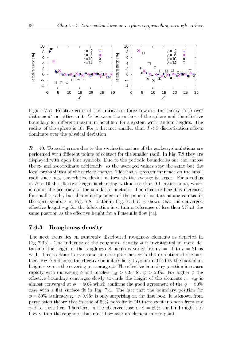
90 Chapter 7. Lubrication force on a sphere approaching a rough surface
-4
-2
0
2 4
6
8
10
0 5 10 15 20 25 30
rela
tive
erro
r [%
]
d*
r = 2r = 6r =10r =14
-4
-2
0
2 4
6
8
10
0 5 10 15 20 25 30
rela
tive
erro
r [%
]
d*
r = 2r = 6r =10r =14
Figure 7.7: Relative error of the lubrication force towards the theory (7.1) overdistance d∗ in lattice units δx between the surface of the sphere and the effectiveboundary for different maximum heights r for a system with random heights. Theradius of the sphere is 16. For a distance smaller than d < 3 discretization effectsdominate over the physical deviation
R = 40. To avoid errors due to the stochastic nature of the surface, simulations areperformed with different points of contact for the smaller radii. In Fig. 7.8 they aredisplayed with open blue symbols. Due to the periodic boundaries one can choosethe x- and z-coordinate arbitrarily, so the averaged values stay the same but thelocal probabilities of the surface change. This has a stronger influence on the smallradii since here the relative deviation towards the average is larger. For a radiusof R > 16 the effective height is changing within less than 0.1 lattice units, whichis about the accuracy of the simulation method. The effective height is increasedfor smaller radii, but this is independent of the point of contact as one can see inthe open symbols in Fig. 7.8. Later in Fig. 7.11 it is shown that the convergedeffective height reff for the lubrication is within a tolerance of less then 5% at thesame position as the effective height for a Poiseuille flow [74].
7.4.3 Roughness density
The next focus lies on randomly distributed roughness elements as depicted inFig 7.3b). The influence of the roughness density φ is investigated in more de-tail and the height of the roughness elements is varied from r = 11 to r = 21 aswell. This is done to overcome possible problems with the resolution of the sur-face. Fig. 7.9 depicts the effective boundary height reff normalised by the maximumheight r versus the covering percentage φ. The effective boundary position increasesrapidly with increasing φ and reaches reff > 0.9r for φ > 20%. For higher φ theeffective boundary converges slowly towards the height of the elements r. reff isalmost converged at φ = 50% which confirms the good agreement of the φ = 50%case with a flat surface fit in Fig. 7.4. The fact that the boundary position forφ = 50% is already reff > 0.95r is only surprising on the first look. It is known frompercolation-theory that in case of 50% porosity in 2D there exists no path from oneend to the other. Therefore, in the observed case of φ = 50% the fluid might notflow within the roughness but must flow over an element in one point.
7.4. Influence of different parameters 91
0
2
4
6
8
10
0 5 10 15 20 25 30 35 40
effe
ctiv
e bo
unda
ry r
eff
radius R
Figure 7.8: Effective height reff versus the radius of the sphere R for a randomlydistributed roughness, at r = 10 and φ = 8%. The blue and open symbols showdifferent points of contact. For radii larger then 16 the effective height is converged.At a radius of R > 40 finite size- and transient effects start to disturb the result.
A good agreement between the two values for r can be seen, demonstrating thatthe resolution has only little influence on the behavior of the measured boundaryposition. Most notably, this even holds if r is larger than the radius of the ap-proached sphere R = 16. The deviation for the low densities has its origin in thestrong variation of the local roughness density and the fact that here the flow withinthe roughness layer is much more dependent on the lower boundary than on theroughness itself. The result shows that a small number of high roughness elementscan have a great influence on the lubrication and leads to the conclusion that theinfluence of surface shape variations has to be very well controlled for high precisionmicrofluidic experiments. This has to be kept in mind when constructing surfacessuch as nanotube forests [66, 37, 7], or generally when dealing with roughness inmicrofluidic systems.
7.4.4 Point of contact
In the following sections systems with a grooved surface are investigated, as depictedin Fig. 7.3c. The main difference between grooves and the random surfaces is thatgrooves are not isotropic. For a Poiseuille flow setup, this means that there aretwo possible flow directions, either in the direction of the grooves (longitudinal)or transversal to the groove structure. For sphere drainage this means that therotational symmetry is broken. A second effect is that the point of contact shouldbecome important now due to the anisotropy, i.e. whether the point of contact is ina ”valley” or on a ”hill”. For the simulations grooves with a squared cross sectionare used. Therefore, the maximum height r and the groove width are identical. Toinvestigate the influence of the variation of the point of contact, simulations areperformed with a constant geometry, but the sphere is moved away from the centerby a distance δ in steps of one lattice unit. As surface grooves with r = 10 arechosen.
Fig. 7.10 right shows the relative deviation δF = F −FMaude/FMaude between the
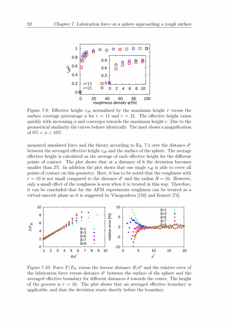
92 Chapter 7. Lubrication force on a sphere approaching a rough surface
0
0.2
0.4
0.6
0.8
1
0 20 40 60 80 100
r eff/
r
roughness density φ [%]
r=11 r=21
0
0.3
0.6
0.9
0 2 4 6 8 10
Figure 7.9: Effective height reff normalized by the maximum height r versus thesurface coverage percentage φ for r = 11 and r = 21. The effective height raisesquickly with increasing φ and converges towards the maximum height r. Due to thegeometrical similarity the curves behave identically. The inset shows a magnificationof 0% < φ < 10%
measured simulated force and the theory according to Eq. 7.1 over the distance d∗
between the averaged effective height reff and the surface of the sphere. The averageeffective height is calculated as the average of each effective height for the differentpoints of contact. The plot shows that at a distance of 6 the deviation becomessmaller than 2%. In addition the plot shows that one single reff is able to cover allpoints of contact on this geometry. Here, it has to be noted that the roughness withr = 10 is not small compared to the distance d∗ and the radius R = 16. However,only a small effect of the roughness is seen when it is treated in this way. Therefore,it can be concluded that for the AFM experiments roughness can be treated as avirtual smooth plane as it is suggested by Vinogradova [150] and Kunert [74].
0
2
4
6
8
10
1 2 3 4 5 6 7 8 9 10
F/F
St
R/d*
δ=1 δ=3 δ=5 δ=7 δ=9
-10
-5
0
5
10
0 5 10 15 20
rela
tive
erro
r [%
]
d*
δ=1 δ=3 δ=5 δ=7 δ=9
Figure 7.10: Force F/FSt versus the inverse distance R/d∗ and the relative error ofthe lubrication force versus distance d∗ between the surface of the sphere and theaveraged effective boundary for different distances δ towards the center. The heightof the grooves is r = 10. The plot shows that an averaged effective boundary isapplicable, and that the deviation starts shortly before the boundary.
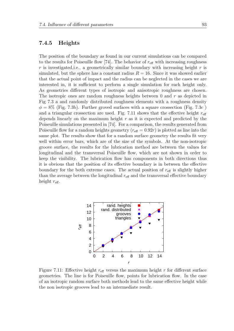
7.4. Influence of different parameters 93
7.4.5 Heights
The position of the boundary as found in our current simulations can be comparedto the results for Poiseuille flow [74]. The behavior of reff with increasing roughnessr is investigated,i.e., a geometrically similar boundary with increasing height r issimulated, but the sphere has a constant radius R = 16. Since it was showed earlierthat the actual point of impact and the radius can be neglected in the cases we areinterested in, it is sufficient to perform a single simulation for each height only.As geometries different types of isotropic and anisotropic roughness are chosen.The isotropic ones are random roughness heights between 0 and r as depicted inFig 7.3 a and randomly distributed roughness elements with a roughness densityφ = 8% (Fig. 7.3b). Further groved surfaces with a square crossection (Fig. 7.3c )and a triangular crossection are used. Fig. 7.11 shows that the effective height reff
depends linearly on the maximum height r as it is expected and predicted by thePoiseuille simulations presented in [74]. For a comparison, the results generated fromPoiseuille flow for a random heights geometry (reff = 0.92r) is plotted as line into thesame plot. The results show that for a random surface geometry the results fit verywell within error bars, which are of the size of the symbols. At the non-isotropicgroove surface, the results for the lubrication method are between the values forlongitudinal and the transversal Poiseuille flow, which are not shown in order tokeep the visibility. The lubrication flow has components in both directions thusit is obvious that the position of its effective boundary is in between the effectiveboundary for the both extreme cases. The actual position of reff is slightly higherthan the average between the longitudinal reff and the transversal effective boundaryheight reff .
0
2
4
6
8
10
12
14
0 2 4 6 8 10 12 14
r eff
r
rand. heightsrand. distributed
groovestriangles
Figure 7.11: Effective height reff versus the maximum height r for different surfacegeometries. The line is for Poiseuille flow, points for lubrication flow. In the caseof an isotropic random surface both methods lead to the same effective height whilethe non isotropic grooves lead to an intermediate result.
94 Chapter 7. Lubrication force on a sphere approaching a rough surface
Resume
In this chapter it is shown that the idea of an effective boundary is applicable evenfor roughness that is not small compared to the radius of the sphere R or the effectivedistance d∗ between the surface of the sphere and the boundary. Further, it is shownthat the effective height reff of the lubrication-based simulations is in good agreementwith the results from Poiseuille flow simulations in chapter 5. Further it was shownthat only a small fraction of roughness elements can result in an effective boundaryclose to the highest point of the asperities.
The results show that surface roughness plays an issue in AFM-based slip exper-iments but it can be treated in an easy manner by shifting the boundary and surfaceposition.
Chapter 8
Super-hydrophobic surfaces
As shown in chapter 3, the combination of hydrophobicity and roughness can lead toso-called super-hydrophobicity. The understanding of this effect is very limited and,both, experimental and analytical approaches, are difficult. Since a large reductionof the friction close to the boundary is expected at super-hydrophobic surfaces, theyare technologically interesting. In the previous chapters the influence of roughnesson the flow close to the surface was discussed. The next step is to investigate whicheffect the combination of roughness and hydrophobicity has on the slip length β.Therefore, it is of interest to investigate the flow over bubbles that are trapped inthe surface topology. In this chapter the construction of super-hydrophobic cells ispresented. A whole surface can be formed by an array of such cells that is realizedby applying periodic boundaries. This enables the discussion of preliminary resultsof fluid flow in the vicinity of such an array of unit cells. A slip effect is found, andcompared to analytical and experimental results.
8.1 Creation of a super-hydrophobic surface in
the lattice Boltzmann method
Before it is possible to investigate the behavior of super-hydrophobic surfaces it isnecessary to find a suitable setup. Due to the improved stability and the lowercomputational effort, a Poiseuille flow setup is chosen. The flow is driven by a forcefx in x direction, which is equivalent to a pressure gradient ∂p
∂x. In z direction simple
periodic boundary conditions are applied. Two surfaces, with a distance in betweenthem of 2d in the y dimension, form the remaining boundary. The upper plane ishydrophilic (i.e. no slip BC) while the lower one consists of one super-hydrophobicunit cell of the length L in x direction. Due to the periodicity only one cell is neededto represent the whole surface. As described in chapter 4 a Shan-Chen model is ableto model a liquid-gas phase-transition. As reminder, in the model a force that isdirected opposed to the density gradient is applied to generate a phase separationbetween a lighter (gas) and a denser (liquid) phase. The Shan-Chen force fSC in asingle component system is given by Eq. 4.64
fSC = Ψ(ρ(x))g∑
i
ciΨ(ρ(x + ci))
95
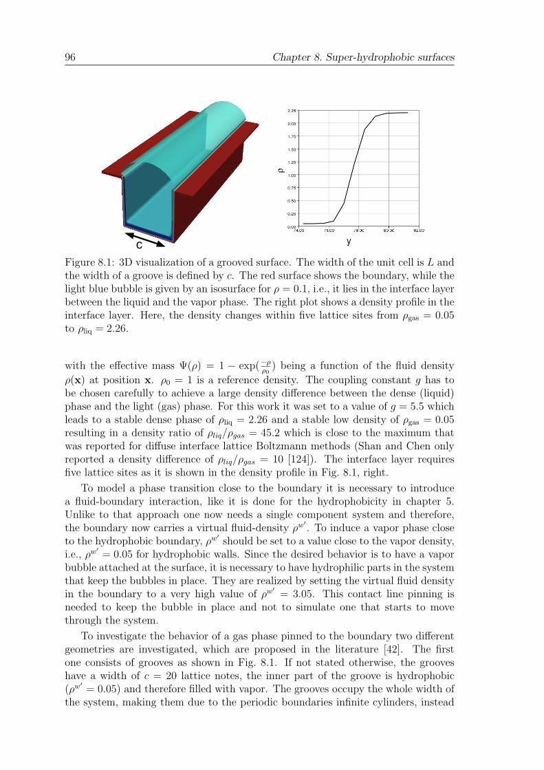
96 Chapter 8. Super-hydrophobic surfaces
cFigure 8.1: 3D visualization of a grooved surface. The width of the unit cell is L andthe width of a groove is defined by c. The red surface shows the boundary, while thelight blue bubble is given by an isosurface for ρ = 0.1, i.e., it lies in the interface layerbetween the liquid and the vapor phase. The right plot shows a density profile in theinterface layer. Here, the density changes within five lattice sites from ρgas = 0.05to ρliq = 2.26.
with the effective mass Ψ(ρ) = 1 − exp(−ρρ0
) being a function of the fluid density
ρ(x) at position x. ρ0 = 1 is a reference density. The coupling constant g has tobe chosen carefully to achieve a large density difference between the dense (liquid)phase and the light (gas) phase. For this work it was set to a value of g = 5.5 whichleads to a stable dense phase of ρliq = 2.26 and a stable low density of ρgas = 0.05resulting in a density ratio of ρliq/ρgas = 45.2 which is close to the maximum thatwas reported for diffuse interface lattice Boltzmann methods (Shan and Chen onlyreported a density difference of ρliq/ρgas = 10 [124]). The interface layer requiresfive lattice sites as it is shown in the density profile in Fig. 8.1, right.
To model a phase transition close to the boundary it is necessary to introducea fluid-boundary interaction, like it is done for the hydrophobicity in chapter 5.Unlike to that approach one now needs a single component system and therefore,the boundary now carries a virtual fluid-density ρw′
. To induce a vapor phase closeto the hydrophobic boundary, ρw′
should be set to a value close to the vapor density,i.e., ρw′
= 0.05 for hydrophobic walls. Since the desired behavior is to have a vaporbubble attached at the surface, it is necessary to have hydrophilic parts in the systemthat keep the bubbles in place. They are realized by setting the virtual fluid densityin the boundary to a very high value of ρw′
= 3.05. This contact line pinning isneeded to keep the bubble in place and not to simulate one that starts to movethrough the system.
To investigate the behavior of a gas phase pinned to the boundary two differentgeometries are investigated, which are proposed in the literature [42]. The firstone consists of grooves as shown in Fig. 8.1. If not stated otherwise, the grooveshave a width of c = 20 lattice notes, the inner part of the groove is hydrophobic(ρw′
= 0.05) and therefore filled with vapor. The grooves occupy the whole width ofthe system, making them due to the periodic boundaries infinite cylinders, instead
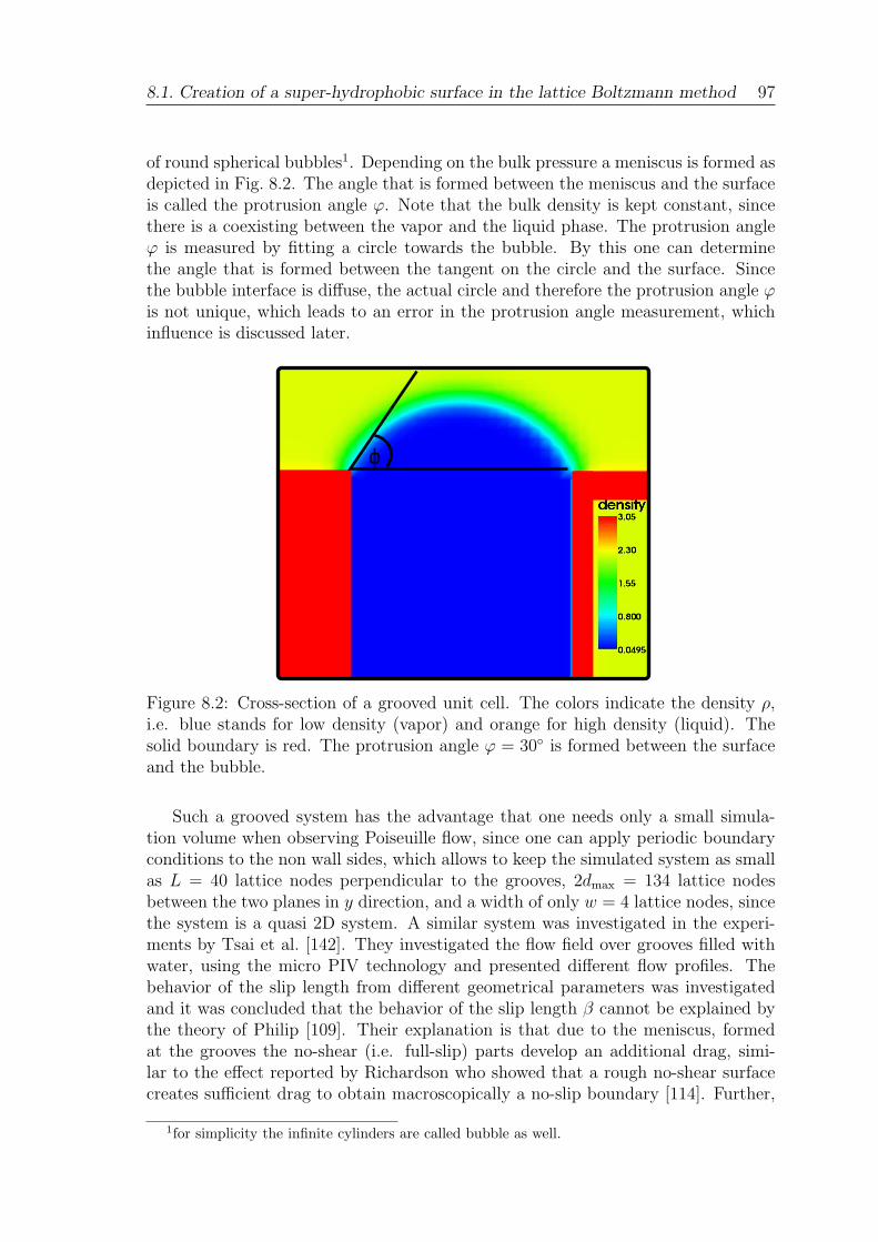
8.1. Creation of a super-hydrophobic surface in the lattice Boltzmann method 97
of round spherical bubbles1. Depending on the bulk pressure a meniscus is formed asdepicted in Fig. 8.2. The angle that is formed between the meniscus and the surfaceis called the protrusion angle ϕ. Note that the bulk density is kept constant, sincethere is a coexisting between the vapor and the liquid phase. The protrusion angleϕ is measured by fitting a circle towards the bubble. By this one can determinethe angle that is formed between the tangent on the circle and the surface. Sincethe bubble interface is diffuse, the actual circle and therefore the protrusion angle ϕis not unique, which leads to an error in the protrusion angle measurement, whichinfluence is discussed later.
ϕ
Figure 8.2: Cross-section of a grooved unit cell. The colors indicate the density ρ,i.e. blue stands for low density (vapor) and orange for high density (liquid). Thesolid boundary is red. The protrusion angle ϕ = 30 is formed between the surfaceand the bubble.
Such a grooved system has the advantage that one needs only a small simula-tion volume when observing Poiseuille flow, since one can apply periodic boundaryconditions to the non wall sides, which allows to keep the simulated system as smallas L = 40 lattice nodes perpendicular to the grooves, 2dmax = 134 lattice nodesbetween the two planes in y direction, and a width of only w = 4 lattice nodes, sincethe system is a quasi 2D system. A similar system was investigated in the experi-ments by Tsai et al. [142]. They investigated the flow field over grooves filled withwater, using the micro PIV technology and presented different flow profiles. Thebehavior of the slip length from different geometrical parameters was investigatedand it was concluded that the behavior of the slip length β cannot be explained bythe theory of Philip [109]. Their explanation is that due to the meniscus, formedat the grooves the no-shear (i.e. full-slip) parts develop an additional drag, simi-lar to the effect reported by Richardson who showed that a rough no-shear surfacecreates sufficient drag to obtain macroscopically a no-slip boundary [114]. Further,
1for simplicity the infinite cylinders are called bubble as well.

98 Chapter 8. Super-hydrophobic surfaces
Davis and Lauga developed a theoretical model valid for grooves covered with no-shear ”bubbles”, to describe the slip length β in dependence on the protrusion angleϕ [32]. The main idea is that there is a no-shear meniscus on a no-slip plane. Insuch a system two opposing effects can be observed: the larger the meniscus gets,the longer the fluid is accelerated, but the stronger the drag becomes due to thesurface roughness created by the bubble. Their main result can be summarizedas follows: there exists a critical protrusion angle ϕc above which the effect of thewall-attached bubbles displays a transition from reduced to enhanced fraction, i.e.the slip length β becomes negative. They predict this angle to be ϕc = 65. Theypredict as well a maximum protrusion angle ϕmax at which the drag reduction ismaximized. This angle depends on the ratio between the no-slip and the no-shearpart, however, for equally long no-slip and no-shear parts the maximum protrusionangle is ϕmax = 25. Interestingly, they predict as well that for negative protrusionangles there is no negative slip length.
Figure 8.3: Illustration of a 3D unit cell for a large bubble. The red surface showsthe boundary, while the light blue bubble is given by an isosurface for ρ = 0.1, i.e.,it lies in the interface layer between the liquid and the vapor phase.
A different, three dimensional, super-hydrophobic cell is given by a circular cylin-drical hole with hydrophobic inner walls. A bubble is formed inside the hole. InFig. 8.3 the red surface shows the boundary of a cylindrical hole with an inner radiusof R = 18 in a 80 × 80 lattice units large cell. The light blue bubble is created byshowing an iso-surface for a density of ρ = 0.1, i.e., a value to depict the interfacelayer between the vapor bubble and the liquid. Such a model was investigated byHyvaluoma and Harting using lattice Boltzmann simulations of Couette flow in thevicinity of such a surface [59]. They found a shear dependent slip length, which hasits origin in the deformation of the meniscus. In contrast to the results by Davisand Lauga they found the maximum slip length at a protrusion angle of ϕmax = 0.However, the qualitative behavior is the same namely that at a critical protrusionangle ϕc ≈ 65 the slip length becomes negative. However, there is a principle dif-ference between the works: Hyvaluoma and Harting investigate 3D structures, whileDavis and Lauga’s calculations are valid for a quasi 2D structure.
To investigate the flow over the presented surfaces, a Poiseuille flow setup ischosen in this chapter. In contrast to the previous chapters one surface consist ofa single super-hydrophobic unit cell and the other surface is a flat no-slip surface.The distance between the two surfaces is chosen as 2d = 134. This distance hasto be large compared to the height of the bubble, because otherwise the bubbledisturbs the bulk flow strongly, making it impossible to define an averaged effect ofthe super-hydrophobicity. The flow is driven by a constant body force. This is a
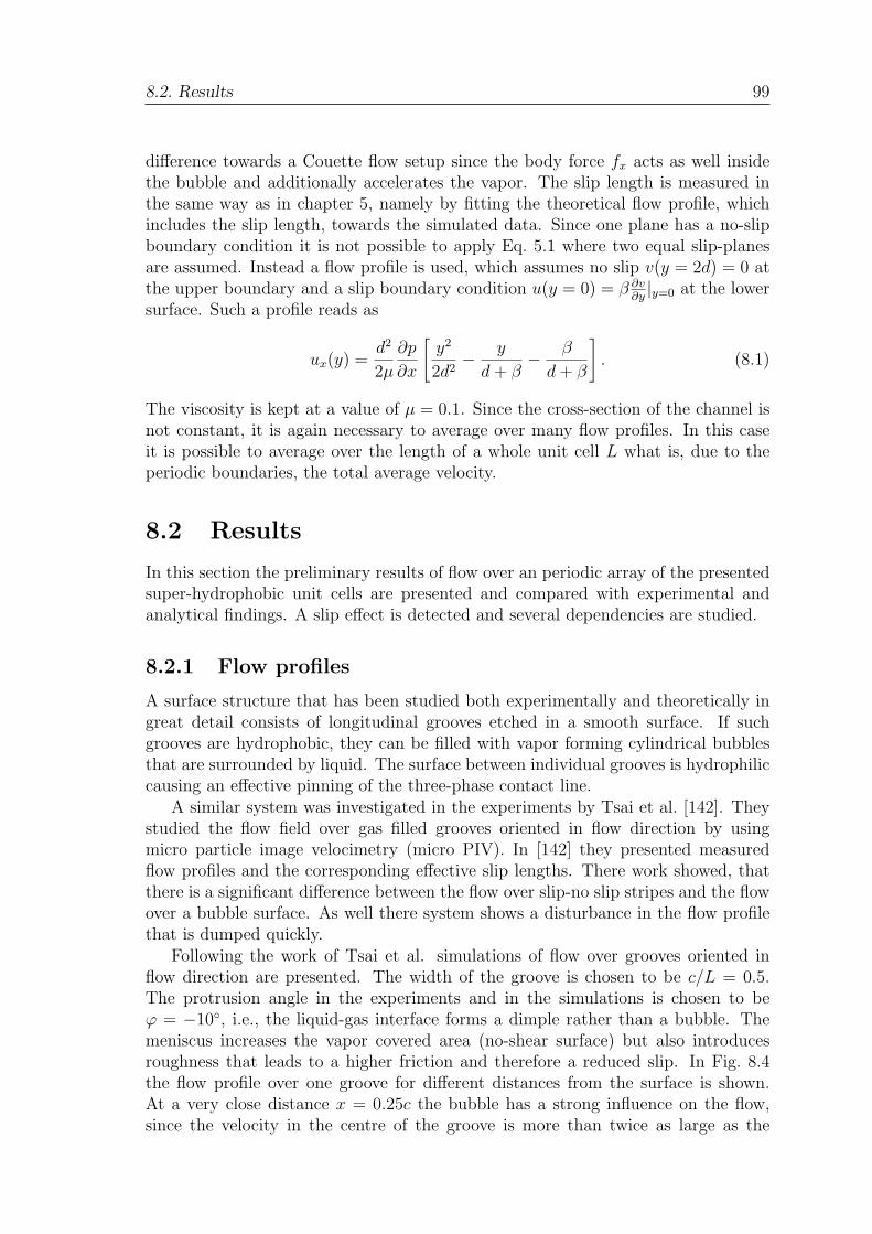
8.2. Results 99
difference towards a Couette flow setup since the body force fx acts as well insidethe bubble and additionally accelerates the vapor. The slip length is measured inthe same way as in chapter 5, namely by fitting the theoretical flow profile, whichincludes the slip length, towards the simulated data. Since one plane has a no-slipboundary condition it is not possible to apply Eq. 5.1 where two equal slip-planesare assumed. Instead a flow profile is used, which assumes no slip v(y = 2d) = 0 atthe upper boundary and a slip boundary condition u(y = 0) = β ∂v
∂y|y=0 at the lower
surface. Such a profile reads as
ux(y) =d2
2µ
∂p
∂x
[
y2
2d2− y
d + β− β
d + β
]
. (8.1)
The viscosity is kept at a value of µ = 0.1. Since the cross-section of the channel isnot constant, it is again necessary to average over many flow profiles. In this caseit is possible to average over the length of a whole unit cell L what is, due to theperiodic boundaries, the total average velocity.
8.2 Results
In this section the preliminary results of flow over an periodic array of the presentedsuper-hydrophobic unit cells are presented and compared with experimental andanalytical findings. A slip effect is detected and several dependencies are studied.
8.2.1 Flow profiles
A surface structure that has been studied both experimentally and theoretically ingreat detail consists of longitudinal grooves etched in a smooth surface. If suchgrooves are hydrophobic, they can be filled with vapor forming cylindrical bubblesthat are surrounded by liquid. The surface between individual grooves is hydrophiliccausing an effective pinning of the three-phase contact line.
A similar system was investigated in the experiments by Tsai et al. [142]. Theystudied the flow field over gas filled grooves oriented in flow direction by usingmicro particle image velocimetry (micro PIV). In [142] they presented measuredflow profiles and the corresponding effective slip lengths. There work showed, thatthere is a significant difference between the flow over slip-no slip stripes and the flowover a bubble surface. As well there system shows a disturbance in the flow profilethat is dumped quickly.
Following the work of Tsai et al. simulations of flow over grooves oriented inflow direction are presented. The width of the groove is chosen to be c/L = 0.5.The protrusion angle in the experiments and in the simulations is chosen to beϕ = −10, i.e., the liquid-gas interface forms a dimple rather than a bubble. Themeniscus increases the vapor covered area (no-shear surface) but also introducesroughness that leads to a higher friction and therefore a reduced slip. In Fig. 8.4the flow profile over one groove for different distances from the surface is shown.At a very close distance x = 0.25c the bubble has a strong influence on the flow,since the velocity in the centre of the groove is more than twice as large as the
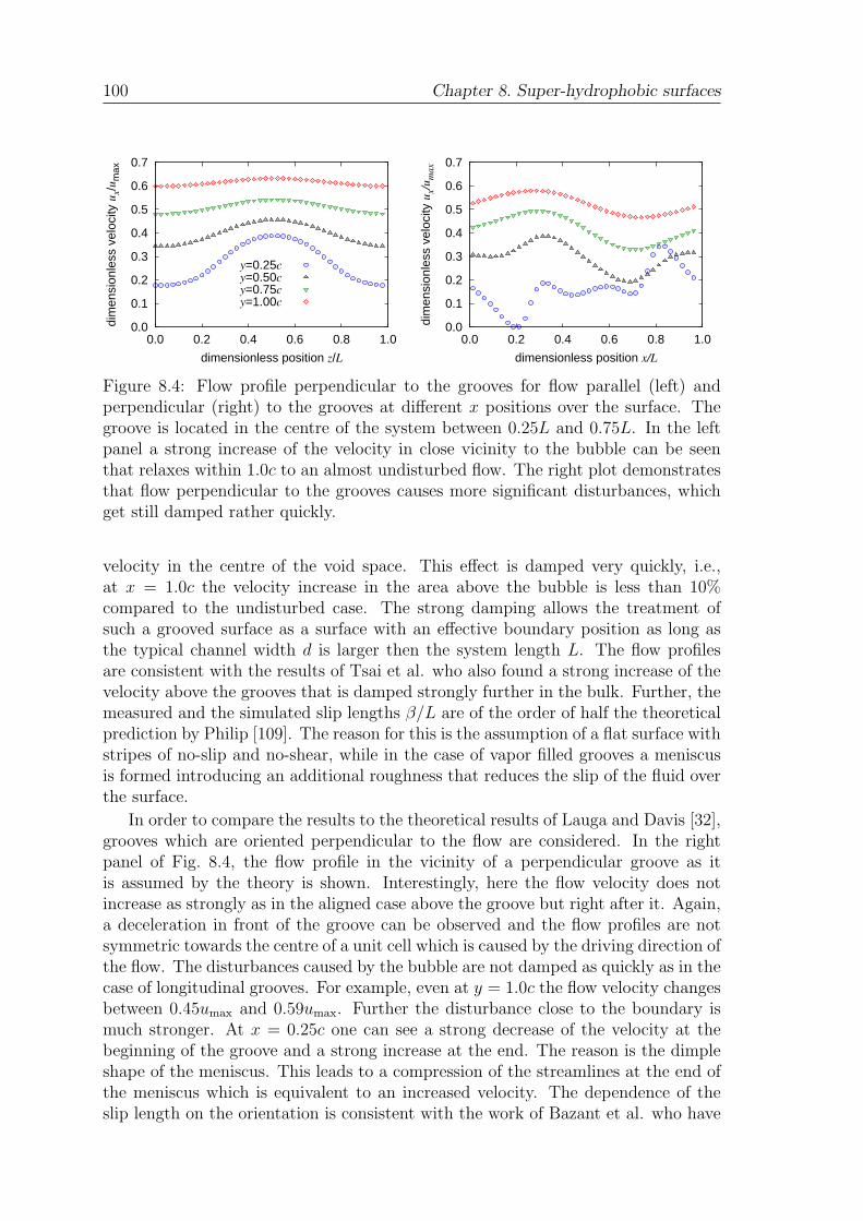
100 Chapter 8. Super-hydrophobic surfaces
0.0
0.1
0.2
0.3
0.4
0.5
0.6
0.7
0.0 0.2 0.4 0.6 0.8 1.0
dim
ensi
onle
ss v
eloc
ity u
x/u
max
dimensionless position z/L
y=0.25cy=0.50cy=0.75cy=1.00c
0.0
0.1
0.2
0.3
0.4
0.5
0.6
0.7
0.0 0.2 0.4 0.6 0.8 1.0
dim
ensi
onle
ss v
eloc
ity u
x/u
max
dimensionless position x/L
Figure 8.4: Flow profile perpendicular to the grooves for flow parallel (left) andperpendicular (right) to the grooves at different x positions over the surface. Thegroove is located in the centre of the system between 0.25L and 0.75L. In the leftpanel a strong increase of the velocity in close vicinity to the bubble can be seenthat relaxes within 1.0c to an almost undisturbed flow. The right plot demonstratesthat flow perpendicular to the grooves causes more significant disturbances, whichget still damped rather quickly.
velocity in the centre of the void space. This effect is damped very quickly, i.e.,at x = 1.0c the velocity increase in the area above the bubble is less than 10%compared to the undisturbed case. The strong damping allows the treatment ofsuch a grooved surface as a surface with an effective boundary position as long asthe typical channel width d is larger then the system length L. The flow profilesare consistent with the results of Tsai et al. who also found a strong increase of thevelocity above the grooves that is damped strongly further in the bulk. Further, themeasured and the simulated slip lengths β/L are of the order of half the theoreticalprediction by Philip [109]. The reason for this is the assumption of a flat surface withstripes of no-slip and no-shear, while in the case of vapor filled grooves a meniscusis formed introducing an additional roughness that reduces the slip of the fluid overthe surface.
In order to compare the results to the theoretical results of Lauga and Davis [32],grooves which are oriented perpendicular to the flow are considered. In the rightpanel of Fig. 8.4, the flow profile in the vicinity of a perpendicular groove as itis assumed by the theory is shown. Interestingly, here the flow velocity does notincrease as strongly as in the aligned case above the groove but right after it. Again,a deceleration in front of the groove can be observed and the flow profiles are notsymmetric towards the centre of a unit cell which is caused by the driving direction ofthe flow. The disturbances caused by the bubble are not damped as quickly as in thecase of longitudinal grooves. For example, even at y = 1.0c the flow velocity changesbetween 0.45umax and 0.59umax. Further the disturbance close to the boundary ismuch stronger. At x = 0.25c one can see a strong decrease of the velocity at thebeginning of the groove and a strong increase at the end. The reason is the dimpleshape of the meniscus. This leads to a compression of the streamlines at the end ofthe meniscus which is equivalent to an increased velocity. The dependence of theslip length on the orientation is consistent with the work of Bazant et al. who have
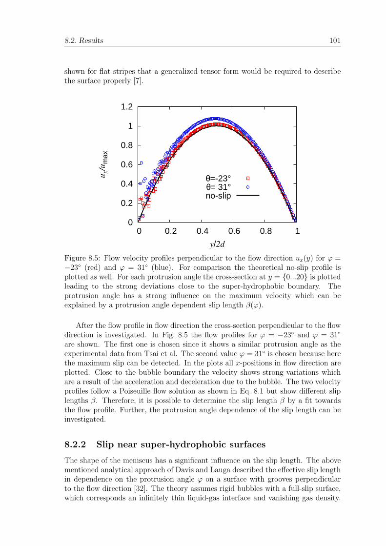
8.2. Results 101
shown for flat stripes that a generalized tensor form would be required to describethe surface properly [7].
0
0.2
0.4
0.6
0.8
1
1.2
0 0.2 0.4 0.6 0.8 1
ux/
um
ax
y/2d
θ=-23°θ= 31°no-slip
Figure 8.5: Flow velocity profiles perpendicular to the flow direction ux(y) for ϕ =−23 (red) and ϕ = 31 (blue). For comparison the theoretical no-slip profile isplotted as well. For each protrusion angle the cross-section at y = 0...20 is plottedleading to the strong deviations close to the super-hydrophobic boundary. Theprotrusion angle has a strong influence on the maximum velocity which can beexplained by a protrusion angle dependent slip length β(ϕ).
After the flow profile in flow direction the cross-section perpendicular to the flowdirection is investigated. In Fig. 8.5 the flow profiles for ϕ = −23 and ϕ = 31
are shown. The first one is chosen since it shows a similar protrusion angle as theexperimental data from Tsai et al. The second value ϕ = 31 is chosen because herethe maximum slip can be detected. In the plots all x-positions in flow direction areplotted. Close to the bubble boundary the velocity shows strong variations whichare a result of the acceleration and deceleration due to the bubble. The two velocityprofiles follow a Poiseuille flow solution as shown in Eq. 8.1 but show different sliplengths β. Therefore, it is possible to determine the slip length β by a fit towardsthe flow profile. Further, the protrusion angle dependence of the slip length can beinvestigated.
8.2.2 Slip near super-hydrophobic surfaces
The shape of the meniscus has a significant influence on the slip length. The abovementioned analytical approach of Davis and Lauga described the effective slip lengthin dependence on the protrusion angle ϕ on a surface with grooves perpendicularto the flow direction [32]. The theory assumes rigid bubbles with a full-slip surface,which corresponds an infinitely thin liquid-gas interface and vanishing gas density.

102 Chapter 8. Super-hydrophobic surfaces
In this case the slip length is given by
β
c= π
(
c
L
)∫ ∞
0A(s)ds, (8.2)
with
A(s) =s
sinh 2s(π − ϕ) + s sin 2ϕ×
[
cos 2ϕ +s sin 2ϕ cosh sπ + sinh s(π − 2ϕ)
sinh sπ
]
.
(8.3)The only parameters entering the calculation of the effective slip length β are theprotrusion angle ϕ and the ratio between the width of a groove c and the length ofa unit cell L. The actual values of the slip length have to be calculated numerically.
0
0.1
0.2
-80 -40 0 40 80
dim
ensi
onle
ss s
lip le
ngth
β /L
protrusion angle ϕ
2% ρlq4% ρlq
50% ρlq90% ρlq
Davis and Lauga
Figure 8.6: Slip length versus protrusion angle ϕ for different threshold values. Thegroove has a width of c = 30 and the system length is L = 40. Since the multiphaselattice Boltzmann model used is a diffuse interface model, the protrusion angle isnot defined uniquely but depends on where the actual interface position is assumed,i.e. which threshold ρt is chosen. Due to the non perfect slip on the vapor phase theanalytical solution by Lauga et al. is scaled down by a factor of 0.75.
In Fig. 8.6 the dimensionless slip length β/L versus the protrusion angle ϕ isshown as given by Eq. 8.2 and by the simulation. The system length in this caseis L = 40 lattice units and the width of a groove is c = 30 lattice units. Since theinterface between the vapor and the liquid is diffuse, the actual bubble position isnot strictly defined. This is in contrast to the theoretical solution and renders thedetermination of the protrusion angle difficult. Therefore, different threshold valuesρt for the fluid density at the interface are chosen to determine the protrusion angle.This value has to be somewhere between the high (liquid) density ρliq = 2.2 and thelower (gas) density ρg = 0.05. In Fig. 8.6 the effect of choosing different thresholdvalues between ρt = 0.02ρliq and 0.9ρliq is demonstrated. Here, it can be observed
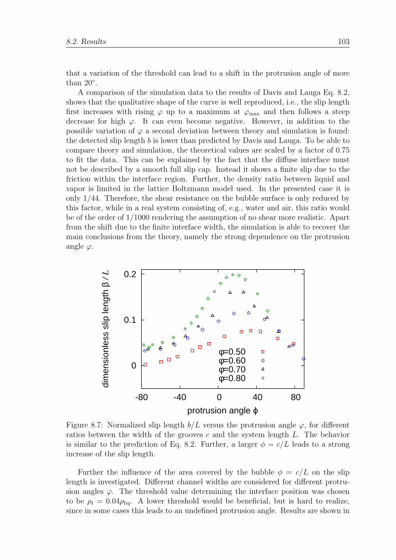
8.2. Results 103
that a variation of the threshold can lead to a shift in the protrusion angle of morethan 20.
A comparison of the simulation data to the results of Davis and Lauga Eq. 8.2,shows that the qualitative shape of the curve is well reproduced, i.e., the slip lengthfirst increases with rising ϕ up to a maximum at ϕmax and then follows a steepdecrease for high ϕ. It can even become negative. However, in addition to thepossible variation of ϕ a second deviation between theory and simulation is found:the detected slip length b is lower than predicted by Davis and Lauga. To be able tocompare theory and simulation, the theoretical values are scaled by a factor of 0.75to fit the data. This can be explained by the fact that the diffuse interface mustnot be described by a smooth full slip cap. Instead it shows a finite slip due to thefriction within the interface region. Further, the density ratio between liquid andvapor is limited in the lattice Boltzmann model used. In the presented case it isonly 1/44. Therefore, the shear resistance on the bubble surface is only reduced bythis factor, while in a real system consisting of, e.g., water and air, this ratio wouldbe of the order of 1/1000 rendering the assumption of no shear more realistic. Apartfrom the shift due to the finite interface width, the simulation is able to recover themain conclusions from the theory, namely the strong dependence on the protrusionangle ϕ.
0
0.1
0.2
-80 -40 0 40 80
dim
ensi
onle
ss s
lip le
ngth
β /
L
protrusion angle ϕ
φ=0.50φ=0.60φ=0.70φ=0.80
Figure 8.7: Normalized slip length b/L versus the protrusion angle ϕ, for differentratios between the width of the grooves c and the system length L. The behavioris similar to the prediction of Eq. 8.2. Further, a larger φ = c/L leads to a strongincrease of the slip length.
Further the influence of the area covered by the bubble φ = c/L on the sliplength is investigated. Different channel widths are considered for different protru-sion angles ϕ. The threshold value determining the interface position was chosento be ρt = 0.04ρliq. A lower threshold would be beneficial, but is hard to realize,since in some cases this leads to an undefined protrusion angle. Results are shown in

104 Chapter 8. Super-hydrophobic surfaces
Fig. 8.7. The qualitative behavior of the results again follows Eq. 8.2. The maximumslip length is increased very strongly by increasing the relative width of the groove.An increase of the surface coverage from φ = 0.5 to 0.8 leads to an increase of thedimensionless slip length where the values for the respective maxima range fromb/L = 0.07 to 0.19. Such a strong increase is also predicted by Eq. 8.2. Further,due to the influence of the increased roughness for ϕ > 60 the slip length becomessmaller for larger ϕ. Also for ϕ < −40 the slip becomes smaller than b < 0.05Land nearly independent on the surface coverage φ.
0
0.01
0.02
0.03
0.04
0.05
0.06
0.01 0.02 0.05 0.1
β/L
umax
Figure 8.8: Normalized slip length β/L versus the maximum flow velocity umax
plotted on a logarithmic scale. Due to the deformation the slip length decreases athigh velocities.
Figure 8.9: Density in a deformed bubble. The white line shows the contour of anundeformed bubble.
Finally, the shear rate dependency of the slip length is analyzed. Hyvaluoma andHarting [59] found a shear dependency due to the deformation of the bubble under
8.2. Results 105
shear, that results in a decreasing slip length. In the Poiseuille flow setup a sheardependency would mean a flow velocity dependency. Therefore, simulations on agroove geometry with different maximum flow velocities ranging from vmax = 0.0001to vmax = 0.12 are performed. As protrusion angle ϕ = 55 is chosen since the bubblehas to range sufficiently far into the system in order to be deformed. Further, the sliplength of β/L = 0.05 in this system is still sufficiently large to see any deviations2.The results are shown in Fig. 8.8. Here, the reduction of the slip length fromβ/L = 0.05 down to β/L = 0.04 is observed. A further reduction could not beobserved for two reasons. The first is that a velocity of umax > 0.12 results in toohigh Mach numbers. Since the lattice Boltzmann method, as it is presented, is onlyvalid for non compressible fluids, the simulation method could not be applied athigher Mach numbers. The second reason is the small deformability of the bubble.To increase it, a larger bubble should be simulated. To show the deformation inFig. 8.9 the density profile for the bubble at vmax = 0.12 is shown. For comparison,an isosurface of the boundary layer of an undeformed bubble is shown as a whiteline. As far as the results can be compared the shear dependency is consistent withthe findings of Hyvaluoma and Harting. In their work the reduction at higher shearrates is more dramatic, because the bubbles are less stiff since they are larger.
Resume
In this chapter Poiseuille flow over super-hydrophobic surfaces is applied to inves-tigate the behavior of the slip length on different parameters. Mainly vapor filledgrooves are investigated which can be compared to the theoretical work of Davisand Lauga [32] and the micro PIV experiments by Tsai et al. [142]. Further, a singlebubble similar to the simulations of Hyvaluoma and Harting [59] is investigated.It was shown that the flow profiles are in good agreement with the experimentalfindings of Tsai et al. [142]. Further, the dependence of the slip length on the pro-trusion angle is compared with the theoretical work. Here, a very good agreementin the critical protrusion angle ϕc and the angle of the maximum slip length ϕmax
was observed. Finally, it is possible to show that a deformation of the bubble undershear leads to a decreased slip length.
2Note that the absolute slip length is β = 0.05 × 40 = 2.0 lattice units

106 Chapter 8. Super-hydrophobic surfaces
Chapter 9
Conclusion
This thesis focuses on lattice Boltzmann simulations of the influence of roughnessand hydrophobicity in microfluidic systems. Therefore, typical experimental setupslike Poiseuille flow and a lubrication force measurement experiment are simulated.Unlike typical idealizations, the investigated surfaces can be randomly rough insteadof being perfectly smooth or having only a simple periodic roughness. Due to this in-creased realism, this work gives a deeper insight, how roughness and hydrophobicityhave to be treated in the data analysis of experiments.
In chapter 3, an overview on the slip phenomenon is given. It can be said that thefield of microfluidics provides a variety of interesting physical phenomena that arehard to describe by analytical theories. Experimental results on slip phenomena areoften inconsistent with each other, which makes a common understanding hard toachieve. Computer simulations can help to draw a clearer picture of slip phenomena.However, the simulation method has to be chosen carefully. Classical CFD methodsneed a founded analytical theory to model sub continuum effects. Since such atheory is missing, they are less helpful in the case of micro-fluidic slip phenomena.Molecular dynamics has the advantage that it can utilize first principles, but suffersform a large computational effort. Therefore, the time and length scales one canachieve by these methods are too small. A possible solution are so-called mesoscopicmethods.
Chapter 4 gives an overview on the lattice Boltzmann (LB) method that is uti-lized in this thesis. By using a discretized version of Boltzmann’s equation, the LBapproach allows to fully resolve the hydrodynamics [129].
Massive particles are described by a continuously moving boundary which is dis-cretized on the lattice. Momentum from the particle to the fluid is transferred suchthat the fluid velocity at the boundary equals the particle’s surface velocity. Sincethe momentum transferred from the fluid to the particle is known, the hydrodynamicforce can be recorded. Hydrophobic interactions and liquid-vapor phase separationare modeled by a Shan-Chen approach. In short, this is a force that is proportionalto the local fluid density and the neighboring, or a virtual boundary density.
By applying a Poiseuille flow setup between rough boundaries, it is possible todemonstrate in chapter 5 that not properly taking into account surface structuresof confining geometries can lead to substantial misinterpretations of measured flowproperties. It is demonstrated that rough surfaces alone can lead to large apparent
107
108 Chapter 9. Conclusion
slip if the distance between boundaries is small [74]. These findings show thatthe concept of an imaginary effective plane where the no-slip boundary conditionis valid, is a good description of a rough boundary. The results are compared toanalytical calculations of Panzer et al. and found to be in good agreement for smallvariations. Large and more realistic perturbations can only be covered by simulationsas presented here. By simulating flow of water along a gold coated surface and arandomly generated one with identical height distribution, it is shown that theposition of the effective plane is independent of the boundary structure and that onlythe height distribution is relevant. Further, these simulations depict the applicabilityof the lattice Boltzmann method to real surface data. Simulations of flow alongsurfaces generated from AFM data allow to determine how detected slip might haveto be corrected to take surface structures into account. Further, it is shown thatthe interplay of roughness and hydrophobicity can lead to both, an increase as wellas decrease of the measured slip length. This can explain the different experimentalfindings concerning the roughness dependency of the slip phenomenon[74, 76, 49].
In chapter 6, finite size and discretization effects of a sphere approaching a flatsurface are investigated. This work is essential for the following investigation utiliz-ing lubrication force measurements. As the solution of Maude (6.4) is reproducible,it demonstrates that at a ratio R/n = 1/32 finite size effects are below 2% and can beneglected near the boundary. It is also demonstrated that a sphere radius of R = 8provides a sufficient resolution. Based on this calibration it is possible to investigatethe influence of different surface properties. Further, the influence of a hydrophobicinteraction between the approached surface and the fluid is investigated. It is shownthat such an interaction leads to a slip with a slip length, which is equivalent tothe one found in a Poiseuille flow setup. The chapter shows to what extent such anapproach is valid. Further, it shows that such lattice Boltzmann simulations haveenough resolution to cover the surface effects that are in the focus of this thesis [77].
Based on these results, it is possible to investigate the influence of roughnesson the lubrication force in chapter 7. The main conclusion is that such a flowis fully equivalent to one which would be created past an effective no-slip smoothsurface, located at the intermediate position between top and bottom of asperities.Its location is controlled by the density of roughness elements but independent onthe flow properties. These results extend the findings of chapter 5.
It is shown that apparent slip created by a hydrophobic surface can be distin-guished from roughness which should be treated as an effective boundary. The ideaof an effective boundary is applicable even for roughness that is not small comparedto the radius of the sphere R or the effective distance d∗ between the surface of thesphere and the boundary. Further, it is shown that the effective height reff of thelubrication based simulations is in agreement with the results from Poiseuille flowsimulations. The results show that surface roughness is an issue in AFM-based slipexperiments, but it can be treated in an easy manner by shifting the boundary andsurface position. The results could have a direct impact on the analysis of SFA/AFMdata and other experimental configurations. In addition, they enable the detectionof measurement artefacts that lead to erroneous conclusions [78].
In chapter 8, Poiseuille flow in the vicinity of super-hydrophobic surfaces is sim-ulated. Preliminary results show that the simulated velocity profiles qualitatively
109
correspond with experimental data of Tsai et al. [142]. The slip length is found todepend on the protrusion angle as predicted from the analytic studies by Davis andLauga [32]. Further, a reduction of the slip length due to the deformation of thebubble at high flow velocities is detected. It is therefore shown that the utilizedsimulation method is able to model super-hydrophobic systems.
For future work different super-hydrophobic surfaces should be investigated.Those could include a model of stiff rods like it is seen in carbon nanotube forests.Other geometries would include grooves with a larger vapor to solid surface ratio.Also more studies on the Wenzel state could be performed were the interplay ofroughness and hydrophobicity is even more crucial. Further some experiments re-port of an increased slip length for increasing shear. It was argued that in this casethe bubbles will not only be deformed, but the contact line will move over the sur-face. Therefore, a non pinned contact line would be a possible continuation of thiswork.
Further, it would be desirable to investigate the influence of a super-hydrophobicsurface on the lubrication force. In such a case, the anisotropy of the grooved surfaceshould influence the results. This is possible in principle, but requires much morecomputer power and larger systems than the current ones. The reason is that it isnecessary to resolve the force curve down to a small fraction of the spheres radius,while having large bubbles on the lattice scale. The bubble, however, may not beentered by the sphere. Therefore, the sphere has to be significantly larger than it isin the presented work for the rough surfaces.
Other super-hydrophobic like behavior could also be created by having a mixtureof two liquids, with the less viscous liquid attracted by the surface. Such a systemcould consist either of water and oil or of polymer melts with an inhomogeneousmolecular weight distribution. In this case, the low viscous fluid would cover thesurface roughness, leading to a drag reduction. In principle, it is possible to simulatethis as well with a lattice Boltzmann model.
In conclusion, it is shown that the effect of roughness and slippage are two distin-guishable phenomena, which are highly related. While roughness leads to a shift ofthe boundary position, slippage, as it can be created by hydrophobic surfaces, leadsto a real increased fluid velocity at the boundary. To obtain a correct descriptionof the boundary condition, both phenomena have to be taken into account. Thisis especially important in the case of so called super-hydrophobic surfaces wherevapor is trapped in the asperities of the surface roughness. It is shown that thelattice Boltzmann method is able to describe such phenomena. Therefore, it canbe used as a tool to design surfaces with special properties like a high slippage orsimulate more complex microfluidic devices, including the complex behavior closeto the boundaries. Further, the findings of this work influence the analysis of slipexperiments which analyze the fundamental question which boundary condition onehas to apply in fluid flow.

110 Chapter 9. Conclusion

Acknowledgments
• Acknowledgements I thank Jens Harting for taking me on as his PhD student,for his help and supervision, and for employing me at the ICP. Further, I wantto thank him for his patience with our papers and my thesis.
• I thank Olga I. Vinogradova for fruitful discussions and the extensive expla-nation of the problems in AFM based slip experiments. I thank Tony Laddfor providing the main parts of the simulation code, for his hospitality at theUniversity of Florida, and for the helpful hints and discussions.
• I thank the DAAD for the scholarship (Doktorandenstipendium) which en-abled me to visit Tony Ladd at the University of Florida. Also, I thank theHPC Europa 2 program for funding my visit at the Eindhoven University ofTechnology (TU/e).
• Special thanks go to the members of all the institutes that I have been to,which are namely the ICP at the University of Stuttgart, the Departmentof Chemical Engineering at the University of Florida, and the MesoscopicTransport Phenomena group at the TU/e. Thanks for the hospitality, thevaluable discussions, and the support.
• The work was financed by the DFG priority program “nano- and microflu-idics” and by the “Landesstiftung Baden-Wurttemberg”. Computations wereperformed at the Neumann Institute for Computing, Julich, at the ScientificSupercomputing Center Karlsruhe, and the ICP condor cluster.
• Last but not least, I want to thank my parents for their support and for givingme the opportunity to go so far.
• And very special thanks to Emily .
111

112 Chapter 9. Conclusion

Bibliography
[1] A. Ajdari and L. Bocquet. Giant amplification of interfacially driven trans-port by hydrodynamic slip: diffusio-osmosis and beyond. Phys. Rev. Lett.,96:186102, 2006.
[2] M. P. Allen and D. J. Tildesley. Computer simulation of liquids. ClarendonPress, 1994.
[3] J. L. Barrat and L. Bocquet. Large slip effect at a nonwetting fluid interface.Phys. Rev. Lett., 82:4671, 1999.
[4] W. Barthlott and C. Neinhuis. The purity of sacred lotus or escape fromcontamination in biological surfaces. Planta, 202:1, 1997.
[5] J. Baudry and E. Charlaix. Experimental evidance for a large slip effect at anonwetting fluid-solid interface. Langmuir, 17:5232, 2001.
[6] O. Baumchen, R. Fetzer, and K. Jacobs. Reduced interfacial entanglementdensity affects the boundary conditions of polymer flow. Physical Review Let-ters, 103(24):247801, 2009.
[7] M. Z. Bazant and O. I. Vinogradova. Tensorial hydrodynamic slip. J. FluidMech., 613:125, 2008.
[8] R. Benzi, L. Biferale, M. Sbragaglia, S. Succi, and F. Toschi. Mesoscopic two-phase model for describing apparent slip in micro-channel flows. Europhys.Lett., 74:651, 2006.
[9] P. L. Bhatnagar, E. P. Gross, and M. Krook. Model for collision processesin gases. I. Small amplitude processes in charged and neutral one-componentsystems. Phys. Rev., 94(3):511, 1954.
[10] L. Bocquet and J. L. Barrat. Hydrodynamic boundary conditions and corre-lation functions of confined fluids. Phys. Rev. Lett., 70(18):2726, 1993.
[11] L. Bocquet and J. L. Barrat. Hydrodynamic boundary conditions, correlationfunctions, and kubo relations for confined fluids. Phys. Rev. E, 49(4):3079,1994.
[12] L. Bocquet and J. L. Barrat. Flow boundary conditions from nano- to micro-scales. Soft Matter, 3:685, 2007.
113
114 Bibliography
[13] E. Bonaccurso, H-J. Butt, and V. S. J. Craig. Surface roughness and hydro-dynamic boundary slip of a Newtonian fluid in a completely wetting system.Phys. Rev. Lett., 90:144501, 2003.
[14] G. E. P. Box and M. E. Muller. A note on the generation of random normaldeviates. Ann. Math. Stat., 29:610, 1958.
[15] ABD Cassie and S. Baxter. Wettability of porous surfaces. Transactions ofthe Faraday Society, 40:546, 1944.
[16] J. T. Cheng and N. Giordano. Fluid flow through nanometer scale channels.Phys. Rev. E, 65:031206, 2002.
[17] J. H. Cho, B. M. Law, and F.Rietord. Dipole-dependent slip on Newtonianliquids at smoothsolid hydrophobic surfaces. Phys. Rev. Lett., 92:166102, 2004.
[18] C-H. Choi and C. J. Kim. Large slip of aqueous liquid flow over a nanoengi-neered superhydrophobic surface. Phys. Rev. Lett., 96:066001, 2006.
[19] C-H. Choi, U. Ulmanella, J. Kim, C-M Ho, and C. J. Kim. Effective slipand friction reduction in nanograted superhydrophobic microchannels. Phys.Fluids, 18:087105, 2006.
[20] C-H. Choi, K. J. Westin, and K. S. Breuer. Apparent slip in hydrophilic andhydrophobic microchannels. Phys. Fluids, 15:2897, 2003.
[21] N. V. Churaev, V. D. Sobolev, and A. N. Somov. Slippage of liquids overlyophobic solid surfaces. J. Colloid Int. Sci., 97:574, 1984.
[22] B. Cichocki, R. B. Jones, R. Kutteh, and E. Wajnryb. Friction and mobilityfor colloidal spheres in Stokes flow near a boundary: The multipole methodand applications. J. Chem. Phys., 112:2548, 2000.
[23] M. Cieplak, J. Koplik, and J. R Banavar. Boundary conditions at a fluid-solidinterface. Phys. Rev. Lett., 86:803, 2001.
[24] C. Cottin-Bizonne, C. Barentin, E. Charlaix, L. Bocquet, and J. L. Barrat.Dynamics of simple liquids at heterogeneous surfaces: molecular dynamicssimulations and hydrodynamic description. Eur. Phys. J. E, 15:427, 2004.
[25] C. Cottin-Bizonne, J. L. Barrat, L. Bocquet, and E. Charlaix. Low-frictionflows of liquid at nanopatterned interfaces. Nature Materials, 2:237, 2003.
[26] C. Cottin-Bizonne, B. Cross, A. Steinberger, and E. Charlaix. Boundary slipon smooth hydrophobic surfaces: intrinsic effects and possible artefacts. Phys.Rev. Lett., 94:056102, 2005.
[27] C. Cottin-Bizonne, S. Jurine, J. Baudry, J. Crassous, F. Restagno, andE. Charlaix. Nanorheology: an investigation of the boundary condition athydrophobic and hydrophilic interfaces. Eur. Phys. J. E, 9:47, 2002.
Bibliography 115
[28] P. V. Coveney and P. Espanol. Dissipative particle dynamics for interactingmulticomponent systems. J. Phys. C., 30:779, 1997.
[29] P. V. Coveney and K. E. Novik. Computer simulations of domain growth andphase separation in two-dimensional binary immiscible fluids using dissipativeparticle dynamics. Phys. Rev. E, 54(5):5134, 1996.
[30] V. S. J. Craig, C. Neto, and D. R. M. Williams. Shear dependent boundaryslip in an aqueous Newtonian liquid. Phys. Rev. Lett., 87:054504, 2001.
[31] D. d Humieres. Multiple relaxation time lattice Boltzmann models in threedimensions. Phil Trans. A, 360:437, 2002.
[32] A.M.J. Davis and E. Lauga. Geometric transition in friction for flow over abubble mattress. Physics of Fluids, 21:011701, 2009.
[33] B. Du, I. Doubaidoulline, and D. Johansmann. Effects of laterally heteroge-neous slip on the resonance properties of quartz crystals imersed in liquids.Langmuir, 20:7794, 2004.
[34] B. Dunweg, U. D. Schiller, and A. J. C. Ladd. Statistical mechanics of thefluctuating lattice Boltzmann equation. Phys. Rev. E, 76:36704, 2007.
[35] B. Dunweg and A. J. C. Ladd. Lattice Boltzmann simulations oft soft mattersystems. Advanced computer simulation approaches for soft matter sciences,3:89, 2008.
[36] P. Espanol and P. Warren. Statistical mechanics of dissipative particle dy-namics. Europhys. Lett., 30(4):191, 1995.
[37] F. Feuillebois, M.Z. Bazant, and O.I. Vinogradova. Effective slip over super-hydrophobic surfaces in thin channels. Phys. Rev. Lett., 102:026001, 2009.
[38] Daan Frenkel and Berend Smit. Understanding Molecular Simulation. Aca-demic Press, 2002. ISBN: 0-12-267351-4.
[39] T. M. Galea and P. Attrad. Molecular dynamics study of the effect of solidroughness on the slip length at the fluid-solid boundary during shear flow.Langmuir, 20:3477, 2004.
[40] J. Gao, W. D. Leuedtke, and U. Landmann. Layering transitions and dynamicsof confined liquid films. Phys. Rev. Lett., 79:705, 1997.
[41] L. Gao and T.K. McCarthty. Contact angle hysteresis explained. Langmuir,22:6234, 2006.
[42] P. Gao and J. J. Feng. Enhanced slip on a patterned substrate due to depinningof contact line. Physics of Fluids, 21(10):102102, 2009.
[43] P. G. de Gennes. On fluid/wall slippage. Langmuir, 18:3413, 2002.
116 Bibliography
[44] I. Ginzburg, F. Verhaeghe, and D. d’Humieres. Study of simple hydrodynamicsolutions with the two-relaxation-time lattice Boltzmann scheme. Commun.Comput. Phys., 3:519, 2008.
[45] I. Ginzburg, F. Verhaeghe, and D. d’Humieres. Two-relaxation-time lat-tice Boltzmann scheme: about parametrization, veloceity pressure and mixedboundary conditions. Commun. Comput. Phys., 3:427, 2008.
[46] M. Gross, F. Varnik, and D. Raabe. Fall and rise of small droplets on roughhydrophobic substrates. Europhys. Lett., 88:26002, 2009.
[47] J. Harting, M. Harvey, J. Chin, and P. V. Coveney. Detection and tracking ofdefects in the gyroid mesophase. Comp. Phys. Com., 165:97, 2005.
[48] J. Harting, C. Kunert, and H.J. Herrmann. Lattice Boltzmann simulations ofapparent slip in hydrophobic microchannels. Europhysics Letters, 75:328–334,2006.
[49] J. Harting, C. Kunert, and J. Hyvaluoma. Lattice Boltzmann simulations inmicrofluidics: probing the no-slip boundary condition in hydrophobic, rough,and surface nanobubble laden microchannels. Microfluidics and Nanofluidics,8:1, 2010.
[50] Y. Hashimoto, Y. Chen, and H. Ohashi. Immiscible real-coded lattice gas.Comp. Phys. Comm., 129:56, 2000.
[51] H. Hasimoto. On the periodic fundamental solution of the Stokes equationsand their application to viscous flow past a cubic array of spheres. J. FluidMech., 5:317, 1959.
[52] X. He, Q. Zou, L. S. Luo, and M. Dembo. Analytic solutions of simple flowsand analysis of non-slip boundary conditions for the lattice Boltzmann BGKmodel. J. Stat. Phys., 87:115, 1997.
[53] M. Hecht, J. Harting, M. Bier, J. Reinshagen, and H. J. Herrmann. Shearviscosity of claylike colloids in computer simulations and experiments. Phys.Rev. E, 74(2):021403, 2006.
[54] M. Hecht, J. Harting, and H. J. Herrmann. Stability diagram for dense sus-pensions of model colloidal particles in shear flow. Phys. Rev. E, 75(5):051404,2007.
[55] M. Hecht, J. Harting, T. Ihle, and H. J. Herrmann. Simulation of claylikecolloids. Phys. Rev. E, 72(1):011408, Jul 2005.
[56] F. J. Higuera, S. Succi, and R. Benzi. Lattice gas dynamics with enhancedcollisions. Europhys. Lett., 9(4):345, 1989.
[57] E. J. Hinch. Pertubation methods. Cambridge Univ. Press., Cambridge, 1991.

Bibliography 117
[58] P. J. Hoogerbrugge and J. M. V. A. Koelman. Simulating microscopic hy-drodynamic phenomena with dissipative particle dynamics. Europhys. Lett.,19(3):155, 1992.
[59] J. Hyvaluoma and J. Harting. Slip flow over structured surfaces with entrappedmicrobubbles. Phys. Rev. Lett., 100:246001, 2008.
[60] T. Ihle and D. M. Kroll. Stochastic rotation dynamics: a Galilean-invariantmesoscopis model for fluid flow. Phys. Rev. E, 63:020201(R), 2001.
[61] T. Ihle and D. M. Kroll. Stochastic rotation dynamics I: formalism, galileaninvariance, Green-Kubo relations. Phys. Rev. E, 67(6):066705, 2003.
[62] T. Inamuro, M. Yoshino, and F. Ogino. A non-slip boundary condition forlattice Boltzmann simulations. Phys. Fluids, 7(12):2928, 1995.
[63] A. Jabbarzadeh, J. D. Atkinson, and R. I. Tanner. Effect of the wall rough-ness on slip and rheological properties of hexadecane in molecular dynamicssimulation of couette shear flow between two sinusoidal walls. Phys. Rev. E,61:690, 2000.
[64] K. M. Jansons. Determination of the macroscopic (partial) slip boundarycondition for a viscous flow over randomly rough surface with perfect slipmicroscopic boundary condition. Phys. Fluids, 31:15, 1987.
[65] J. E. Jones. On the determination of molecular fields. ii. from the equation ofstate of a gas. Proc. R. Soc. Lond. A, 463:463, 1924.
[66] P. Joseph, C. Cottin-Bizonne, J. M. Benoit, C. Ybert, C. Journet, P. Tabeling,and L. Bocquet. Slippage of water past superhydrophobic carbon nanotubeforests in microchannels. Phys. Rev. Lett., 97:156104, 2006.
[67] P. Joseph and P. Tabeling. Direct measurement of the apparent slip length.Phys. Rev. E, 71:035303, 2005.
[68] M. Junk, A. Klar, and L.-S. Luo. Asymptotic analysis of the lattice Boltzmannequation. J. Comp. Phys., 210:676, 2005.
[69] G. Karniadakis, A. Beskok, and N. Aluru. Microflows and nanoflows, funda-mentals and simulation. Springer, 2005.
[70] M. Knudsen. Experimentelle Bestimmung des Druckes gesattigter Quecksil-berdampfe bei 0o und hoheren Temperaturen. Ann. d. Phys., 29:179, 1909.
[71] J. Koplik and J. R Banavar. No-slip condition for a mixture of two liquids.Phys. Rev. Lett., 80(23):5125, 1998.
[72] J. Koplik, J. R. Banavar, and J. F. Willemsen. Molecular dynamics of fluidflow at solid-surfaces. Phys. Fluids, 1:781, 1989.
118 Bibliography
[73] J. Krim. Friction at macroscopic and microscopic length scales. Am. J. Phys.,70:890, 2002.
[74] C. Kunert and J. Harting. Roughness induced boundary slip in microchannelflows. Phys. Rev. Lett., 99:176001, 2007.
[75] C. Kunert and J. Harting. On the effect of surfactant adsorption and viscositychange on apparent slip in hydrophobic microchannels. Prog. Comp. Fluid.Mech., 8:197, 2008.
[76] C. Kunert and J. Harting. Simulation of fluid flow in hydrophobic roughmicrochannels. In International Journal of Computational Fluid Dynamics,volume 22, page 475, 2008.
[77] C. Kunert and J. Harting. Calibration of lubrication force measurements bylattice Boltzmann simulations. In Proceedings of the 2nd Micro and NanoFlows Conference (2009), 2009.
[78] C. Kunert, J. Harting, and O.I. Vinogradova. Simulations of film drainageto probe random-roughness boundary conditions. Submitted for publication,2009. arxiv:0912.1538.
[79] L. D. Landau and E. M. Lifschitz. Hydrodynamik. Akademieverlag, Berlin,1966.
[80] A. J. C. Ladd. Numerical simulations of particulate suspensions via a dis-cretized Boltzmann equation. part 1. theoretical foundation. J. Fluid Mech.,271:285, 1994.
[81] A. J. C. Ladd. Numerical simulations of particulate suspensions via a dis-cretized Boltzmann equation. part 2. numerical results. J. Fluid Mech.,271:311, 1994.
[82] A. J. C. Ladd and R. Verberg. Lattice-Boltzmann simulations of particle-fluidsuspensions. J. Stat. Phys., 104:1191, 2001.
[83] L. D. Landau and E. M. Lifshitz. Fluid mechanics. Pergamon Press, 1959.
[84] J. Latt and B. Chopard. A benchmark case for lattice Boltzmann: turbulentdipole-wall collision. Int. J. Mod. Phys. C, 18:619, 2007.
[85] J. Latt, B. Chopard, O. Malaspinas, M. Deville, and A. Michler. Straightvelocity boundaries in the lattice Boltzmann method. Phys. Rev. E, 77:056703,2008.
[86] E. Lauga, M. P. Brenner, and H. A. Stone. Microfluidics: the no-slip bound-ary condition. In C. Tropea, A. Yarin, and J. F. Foss, editors, Handbook ofExperimental Fluid Dynamics, chapter 19, pages 1219–1240. Springer, NY,2007.
Bibliography 119
[87] E. Lauga and H. A. Stone. Effective slip in pressure driven flow. J. Fluid.Mech., 489:55, 2003.
[88] N. Lecoq, R. Anthore, B. Cickhocki, P. Szymczak, and F. Feuillebois. Dragforce on a sphere moving towards a corrugated wall. J. Fluid Mech., 513:247,2004.
[89] N. Lecoq, K. Masmoudi, R. Anthore, and F. Feuillebois. Creeping motionof a sphere along the axis of a closed axisymetric container. J. Fluid Mech.,585:127, 2007.
[90] R. Lindken, M. Rossi, Große S, and J. Westerweel. Micro-particle imagevelocimetry: Recent developments, applications, and guidelines. Lab Chip,9:2551, 2009.
[91] D. Lumma, A. Best, A. Gansen, F. Feuillebois., J. O. Radler, and O. I. Vino-gradova. Flow profile near a wall measured by double-focus fluorescence cross-correlation. Phys. Rev. E, 67:056313, 2003.
[92] A. Malevanets and R. Kapral. Continuous-velocity lattice-gas model for fluidflow. Europhys. Lett., 44(5):552, 1998.
[93] A. Malevanets and R. Kapral. Solute molecular dynamics in a mesoscalesolvent. J. Chem. Phys., 112(18):7260, 2000.
[94] C. A. Marsh and P. V. Coveney. Detailed balance and H-theorems for dissi-pative particle dynamics. J. Phys. C., 31:6561, 1998.
[95] A. D. Maude. End effects in a falling-sphere viscometer. British J. Appl.Phys., 12:293, 1961.
[96] J. C. Maxwell. On stresses in rarified gases arising from inequalities of tem-perature. Phil Trans. Roy Soc. Lond., 70:287, 1879.
[97] D. Maynes, K. Jeffs, B. Woolford, and B. W. Webb. Laminar flow in a mi-crochannel with hydrophobic surface patterned microribis oriented parallel tothe flow direction. Phys. Fluids, 19:093603, 2007.
[98] G. McHale and M. I. Newton. Surface roughness and interfacial slip boundarycondition for quarzcrystal microbalances. J. Appl. Phys., 95:373, 2004.
[99] G. R. McNamara and G. Zanetti. Use of the Boltzmann equation to simulatelattice-gas automata. Phys. Rev. Lett., 61(20):2332, 1988.
[100] A. Narvaez, T. Zauner, F. Raischel, R. Hilfer, and J. Harting. lattice-Boltzmann simulations for permeability calculations in porous media. INPREPARATION, 2009.
[101] C. L. M. H. Navier. Memoire sur les lois du mouvement de fluids. Mem. Acad.Sci. Ins. Fr., 6:389, 1823.
120 Bibliography
[102] M. Nekovee and P. V. Coveney. Lattice Boltzmann simulations of self assemblyof binary amphiphilic fluids into ordered lamellar and bicontinous cubic phases.J. Am. Chem. Soc., 123(49):12380, 2001.
[103] C. Neto, V. S. J. Craig, and D. R. M. Williams. Evidence of shear-dependentboundary slip in Newtonian liquids. Eur. Phys. J. E, 12:71, 2003.
[104] C. Neto, D. R. Evans, E. Bonaccurso, H. J. Butt, and V. S. J. Craig. Boundaryslip in Newtonian liquids: a review of experimental studies. Rep. Prog. Phys.,68:2859, 2005.
[105] N. Q. Nguyen and A. J. C. Ladd. Lubrication corrections for lattice-Boltzmannsimulations of particle suspensions. Phys. Rev. E, 66(4):046708, October 2002.
[106] X. Nie, G. D. Doolen, and S. Chen. Lattice-Boltzmann simulations of fluidflows in MEMS. J. Stat. Phys., 107:279, 2002.
[107] J. Ou and G. R. Rothstein. Direct velocity measurement of flow past drag-reducing ultrahydrophobic surfaces. Phys. Fluids, 17:03606, 2005.
[108] P. Panzer, M. Liu, and D. Einzel. The effects of boundary curvature on hydro-dynamic fluid flow: calculation of slip lengths. Int. J. Mod. Phys. B, 6:3251,1992.
[109] J. R. Philip. Flow satisfying mixed no-slip and no-shear conditions. J. Appl.Math. Phys., 23:353, 1972.
[110] R. Pit, H. Hervert, and L. Leger. Direct experimental evidence of slip inhexadecane:solid interface. Phys. Rev. Lett., 85:980, 2000.
[111] N. V. Priezjev, A. A. Darhuber, and S. M. Troian. Slip behavior in liquidfilms on surfaces of patterned wettability: Comparison between continuumand molecular dynamics simulations. Phys. Rev. E, 71:041608, 2005.
[112] Y.H. Qian, D. d’Humieres, and P. Lallemand. Lattice BGK models for Navier-Stokes equation. Europhys. Lett., 17:479, 1992.
[113] R. Rabenseifner. Parallel programing workshop; introduction to computationalfluid dynamics. HLRS Stuttgart, 2005.
[114] S. Richardson. On the no-slip boundary condition. J. Fluid Mech., 59:707,1973.
[115] J.P. Rothstein. Slip on superhydrophobic surfaces. Annu. Rev. Fluid Mech.,42:89, 2010.
[116] T. Sakai, Y. Chen, and H. Ohashi. Formation of micelle in the real-codedlattice gas. Comp. Phys. Comm., 129(1–3):75, 2000.
[117] M. Sbragaglia, R. Benzi, L. Biferale, S. Succi, and F. Toschi. Surfaceroughness-hydrophobicity coupling in microchannel and nanochannel flows.Phys. Rev. Lett., 97:204503, 2006.
Bibliography 121
[118] M. Sbragaglia and A. Prosperetti. A note on the effective slip properties formicrochannel flows with ultrahydrophobic surfaces. Phys. Fluids, 17:043603,2007.
[119] H. Schlichting. Boundary-layer theory. McGraw-Hill, 1979.
[120] T. Schmatko, H. Hervert, and L. Leger. Friction and slip at simple fluid-solidinterfaces. the roles of the molecular shape and the solid liquid interaction.Phys. Rev. Lett., 94:244501, 2005.
[121] S. Schmieschek and J. Harting. Contact angle determination in multicompo-nent lattice boltzmann simulations. arXiv:0910.3915v1, 2009.
[122] E. Schnell. Slippage of water over nonwettable surface. J. Appl. Phys., 27:1149,1956.
[123] F. Schwabl. Statistische Mechanik. Springer, 2000.
[124] X. Shan and H. Chen. Lattice Boltzmann model for simulating flows withmultiple phases and components. Phys. Rev. E, 47(3):1815, 1993.
[125] X. Shan and H. Chen. Simulation of nonideal gases and liquid-gas phasetransitions by the lattice Boltzmann equation. Phys. Rev. E, 49(4):2941, 1994.
[126] X. Shan and G. Doolen. Multicomponent lattice-Boltzmann model with in-terparticle interaction. J. Stat. Phys., 81(112):379, 1995.
[127] P. A. Skordos. Initial and boundary conditions for the lattice Boltzmannmethod. Phys. Rev. E, 48:4823, 1993.
[128] A. Strook, S. K. W. Dertinger, A. Ajdari, I. Mezic, H. A. Stone, and G. M.Whitesides. Chaotic mixer for microchannels. Science, 295:647, 2002.
[129] S. Succi. The lattice Boltzmann equation for fluid dynamics and beyond. Ox-ford University Press, 2001.
[130] S. Succi. Mesoscopic modeling of slip motion at fluid-solid interfaces withheterogeneous catalysis. Phys. Rev. Lett., 89:064502, 2002.
[131] M. C. Sukop and D. T. Thorne Jr. Lattice Boltzmann modeling. Springer,2007.
[132] G. Sun, E. Bonaccurso, V. Franzand, and H. J. Butt. Confined liquid: simul-taneous observation of a moleculary layer structure and hydrodynamic slip. J.Chem Phys., 117:10311, 2002.
[133] M. R. Swift, E. Orlandini, W. R. Osborn, and J. M. Yeomans. Lattice-Boltzmann simulations of liquid-gas and binary fluid mixtures. Phys. Rev.E, 54(5):5041, 1996.
[134] M. R. Swift, W. R. Osborn, and J. M. Yeomans. Lattice Boltzmann simulationof nonideal fluids. Phys. Rev. E, 75(5):830, 1995.

122 Bibliography
[135] P. A. Thompson and M. O. Robbins. Shear flow near solids: epitaxial orderand flow boundary conditions. Phys. Rev. A, 41:6830, 1990.
[136] P. A. Thompson and S. Troian. A general boundary condition for liquid flowat solid surfaces. Nature, 389:360, 1997.
[137] P. A. Tompson and S. M. Trojan. A general boundary condition for liquidflow at solid surfaces. Nature, 389:360, 1997.
[138] D. C. Tretheway and C. D. Meinhart. Apparent fluid slip at hydrophobicmicrochannel walls. Phys. Fluids, 14:L9, 2002.
[139] D. C. Tretheway and C. D. Meinhart. A generating mechanism for apparentslip in hydrophobic microchannels. Phys. Fluids, 15:1509, 2004.
[140] D. C. Tretheway, L. Zhu, L. Petzold, and C. D. Meinhart. Examination ofthe slip boundary condition by micro-PIV and lattice Boltzmann simulations.Proc. of IMECE, 2002.
[141] R. Truesdell, A. Mammoli, P. Vorobieff, P. van Swol, and C. J. Brinker.Drag reduction on a patterned superhydrophobic surface. Phys. Rev. Lett.,97:044504, 2006.
[142] P. Tsai, A. M. Peters, C. Pirat, M. Wessling, R. G. H. Lammertink, andD. Lohse. Quantifying effective slip length over micropatterned hydrophobicsurfaces. Physics of Fluids, 21:112002, 2009.
[143] O. B. Usta, A. J. C. Ladd, and J. E. Butler. Lattice-Boltzmann simulationsof the dynamics of polymer solutions in periodic and confined geometries.J.Chem. Phys., 122:094902, 2005.
[144] F. Varnik, D. Dorner, and D. Raabe. Roughness-induced flow instability: Alattice Boltzmann study. J. Fluid Mech., 573:191, 2007.
[145] R. Verberg and A. J. C. Ladd. Accuracy and stability of a lattice-Boltzmannmodel with subgrid scale boundary conditions. Phys. Rev. E, 65:016701, 2001.
[146] O. I. Vinogradova. Drainage of a thin film confined between hydrophobicsurfaces. Langmuir, 11:2213, 1995.
[147] O. I. Vinogradova. Possible implications of hydrophopic slippage on the dy-namic measurements of hydrophobic forces. J. Phys. Cond. Mat., 8:9491, 1996.
[148] O. I. Vinogradova, K. Koynov, A. Best, and F. Feuillebois. Direct mea-surements of hydrophobic slippage using double-focus fluorescence cross-correlation. Physical Review Letters, 102:118302, 2009.
[149] O. I. Vinogradova and G. E. Yakubov. Dynamic effects on force mesurements.2. lubrication and the atomic force microscope. Langmuir, 19:1227, 2003.
Bibliography 123
[150] O. I. Vinogradova and G. E. Yakubov. Surface roughness and hydrodynamicboundary conditions. Phys. Rev. E, 73:045302(R), 2006.
[151] Y. Wang, B. Bhushan, and A. Maali. Atomic force microscopy measurementof boundary slip on hydrophilic, hydrophobic, and superhydrophobic surfaces.27:754, 2009.
[152] D. E. Weidner and L. W. Schwartz. Contact-line motion of shear-thinningliquids. Physics of Fluids, 6:3535–3538, 1994.
[153] R. N. Wenzel. Resistance of solid surfaces to wetting by water. Ind. Eng.Chem., 28:988, 1936.
[154] S. C. Yang and L. B. Fang. Effect of surface roughness on slip in hydrophobicand hydrophilic microchannels by molecular dynamics simulation. MolecularSimulation, 31:971, 2005.
[155] T. Young. An essay on the cohesion of fluids. Philos. Trans. R. Soc. London,95:65, 1805.
[156] Y. Zhu and S. Granick. Rate-dependent slip of Newtonian liquid at smoothsurfaces. Phys. Rev. Lett., 87:096105, 2001.
[157] Y. Zhu and S. Granick. Limits of the hydrodynamic no-slip boundary condi-tion. Phys. Rev. Lett., 88(10):106102, 2002.
[158] Y. Zhu and S. Granick. No-slip boundary condition switches to partial slipwhen fluid contains surfactant. Langmuir, 18:10058, 2002.