Main points to be covered

• Measures of association in case-control studies

• Prevalent controls design: odds ratio vs. relative risk and the rare disease assumption

• Case-cohort design: odds ratio = relative risk = risk ratio

• Nested case-control design: odds ratio = relative rate = rate ratio

• Odds ratio with multi-level predictor variable

Relative Rate

• Ratio of two person-time rates

• Denominators of two person-time rates must be in the same units

• Frequently described as a type of relative risk but should be distinguished

• Relative hazard from proportional hazards regression is a relative rate

Study Design and Measures of Association

• A well-designed case-control study is an efficient way to observe the disease experience of a cohort or a study base

• Some case-control designs can estimate the same measures of association obtained in a cohort design

Measure of Association in Case-Control Studies

• Odds ratio (OR) of exposure in cases and controls is the measure of association in case-control studies

• OR of exposure = OR of disease

• OR of exposure estimates different measures of association depending on the type of sampling used for the case-control designs

Abbreviations

1= exposed and 0 = not exposed

E1 = Events = diagnoses in exposed group

E0 = Events = diagnoses in unexposed group

N1 = number of persons in exposed group

N0 = number of persons in unexposed group

E1 E1 x N0

RR = N1 = E0 N1

E0

N0

Relative risk in a cohort study where1= exposed and 0 = not exposed

So if you know the ratio E1 , youonly need N0 E0

N1 to calculate RROnly need the ratios, not actual numbers

Measures of association in case-control versus cohort design

• If the study base has been accurately identified, the cases in a case-control study will be the same cases that occur in a cohort study

• Therefore, E1 and E0 can be the same in a cohort study and a case-control study

• If case-control study randomly samples cases,

the ratio E1 will still be the same as in the cohort.

E0

Sampling in a case-control study

• Goal of case-control design: sample the study base to get an unbiased estimate of the exposure distribution in the controls

• If can sample the study base to get an unbiased estimate of the ratio N0

N1

can estimate relative risk (risk ratio) with

case-control design

Three Case-Control Designs

1) Prevalent controls: controls sampled from non-cases at one point in time

2) Case-cohort design: controls sampled from baseline of a cohort or study base

3) Incidence-density controls: design with controls sampled from risk sets of a cohort or study base each time a case is diagnosed

Text example of case-control design showing sampling prevalent controls from non-casesStudy

Base

Only non-casesare eligible to becontrols in thisdesign

Sampling controls from non-cases at end of follow-up

Disease No disease

Exposed a

c ds

(a + b)

(c + d)Unexposed

Disease

bs

No disease

time

In case-control design with prevalent sampling of controls, controls are a sample only of the b and d groups from the study base--no case can be included

cases controls

Inability to calculate relative risk if controls sampled from non-cases

If only non-cases are used to select controls,cannot reconstruct the prevalence of exposure in the original study base.

E1 ratio is known in all case-control designsE0

But sampling only non-cases cannot get unbiased estimate of N0

N1

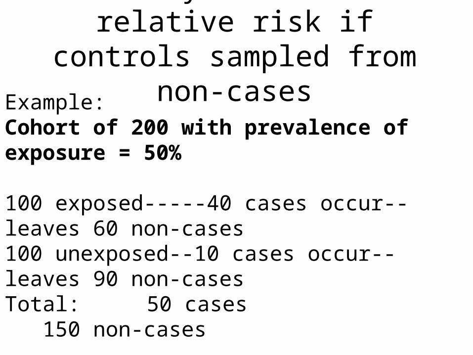
Inability to calculate relative risk if controls sampled from non-cases

Example:Cohort of 200 with prevalence of exposure = 50%

100 exposed-----40 cases occur--leaves 60 non-cases100 unexposed--10 cases occur--leaves 90 non-casesTotal: 50 cases 150 non-cases RR=40/100 / 10/100=4.0

Relative Risk Notation

E1 E1 x N0

RR = N1 = E0 N1

E0

N0

Inability to calculate relative risk: Case-control study with 50 cases

Random sample of 50 controls = 20 exp, 30 no-expE1 = 40 and E0 = 10, so E1 = 4 = 4 E0 1No way to estimate N0 with the cases and controls. N1

If use both cases and controls, N0 = 40 = 0.67 and RR = 4 x 0.67 = 2.7 N1 60

If use controls only, N0 = 30 = 1.5 and RR = 4 x1.5 = 6.0 N1 20 True RR = 4 x 1.0 = 4.0

Case-Control with prevalent controls• If controls are selected among those without disease

at time of study (+ prevalent cases), OR approximates RR only with rare disease assumption

• Rare disease assumption: if incidence of disease low in both groups (<10%), OR RR

• Exposure in controls exposure in whole cohort• Older texts describe case-control design as always

requiring rare disease assumption to estimate RR--not the case

To determine the risk factors associated with toxic-shock syndrome (TSS) in menstruating women, we conducted a retrospective telephone study of 52 cases and 52 age-matched and sex-matched controls. Fifty-two cases and 44 controls used tampons (P=0.02). Moreover,in case-control pairs in which both women used tampons, cases weremore likely than controls to use tampons throughout menstruation (42of 44 vs. 34 of 44, respectively; P=0.05). There were no significantdifferences in brand of tampon used, degree of absorbency specifiedon label, frequency of tampon change, type of contraceptive used, frequency of sexual intercourse, or sexual intercourse during menstruation. Fourteen of 44 cases had one or more definite or probable recurrences during a subsequent menstrual period. In a separate study, Staphylo-coccus aureus was isolated from 62 of 64 women with TSS and from seven of 71 vaginal cultures obtained from healthy controls (P<0.001).Shands KN et al. Toxic-shock syndrome in menstruating women: association with tampon use and Staphylococcus aureus and clinical features in 52 cases. N Engl J Med 1980 Dec 18;303(25):1436-42

Example of Case-Control Study with Prevalent Sampling

Case-control designs with other sampling methods

• Two major alternatives to sampling controls only from prevalent non-cases– Incidence density sampling– Case-cohort sampling

• Both provide valid ways to estimate the exposure distribution in the underlying study base

Case-cohort design: sample baseline of cohort

Case-cohort Sampling• Control group is random sample of cohort at baseline• Gives an unbiased estimate of the prevalence of

exposure in the study base– also useful for calculating attributable risk– control group can be used for >1 disease outcome

• OR = RR (relative risk)• New study design (Prentice, 1986) now being

extended from cohorts to primary study bases

Case-cohort design in primary study base

New residentsPrimaryStudyBase

Quick Method of getting Odds in a 2 x 2 Table:ratio of two cells in column (or row)

Cases Controls

Exp

osur

e

Yes

No

a b

c d

exposure odds in casesis a/c; exposure odds in controls is b/d; and exposure oddsfor all is (a+b)/(c+d)

In a cohort, OR of exposure in cases divided by OR of exposure in whole cohort = relative risk (RR)

Disease No disease

Exposed a

c d

(a + b)

(c + d)UnexposedDisease

b

No disease

time

Exp. odds cases = a Exp. odds cohort = (a+b) OR = a c (c+d) cMultiply both by c = a = RR (a+b) (a+b) (a+b) (c+d) c (c+d)

Odds of exposure in Case-Cohort Sampling

Disease No disease

Exposed a

c d

(a + b)

(c + d)Unexposed

Disease

b

No disease

time

So if sampling is unbiased: (as + bs ) = (a+b) (except for sampling error), (cs + ds ) (c+d) and OR exposure in cases and control group = Relative Risk(NB - control group can contain cases)

Sample for controls (as + bs )

Sample for controls (cs + ds )

Example of case-cohort studyIn the Netherlands Cohort Study among 120,852 subjects aged 55-69 years at baseline (1986), the association between vitamins and carotenoids intake, vitamin supplement use, and bladder cancer incidence was examined. . . . After 6.3 years of follow-up, data from 569 cases and 3123 subcohort members were available for case-cohort analyses. The age-, sex-, and smoking-adjusted relative risks (RRs)for retinol, vitamin E, folate, a-carotene, b-carotene, lutein and zeaxanthin, and lycopene were 1.04, 0.98, 1.03, 0.99, 1.16, 1.11, and1.08, respectively, comparing highest to lowest quintile of intake. Onlyvitamin C (RR: 0.81, 95% CI: 0.61-1.07, P-trend = 0.08), and b-cryptoxanthin intake (RR: 0.74, 95% CI: 0.53-1.03, P-trend =0.01) were inversely associated with bladder cancer risk.

Zeegers MP, Goldbohm RA, Brandt PA. Are retinol, vitamin C, vitamin E, folate and carotenoids intake associated withbladder cancer risk? Results from the Netherlands Cohort Study. Br J Cancer 2001 Sep;85(7):977-83

Third type of case-control sampling

• Incidence density sampling (either in closed cohort = classic nested study or in open primary study base)

• Controls are sampled from the risk set at the time each case is diagnosed

• OR of exposure = rate ratio = relative rate

Nested Case-Control Study with incidence densitysampling within a Cohort Study

Controls Sampled each time a Case is diagnosed = Incidence Density

Incidence Density Sampling in a Primary Study Base (e.g., San Francisco County)

New residents

Nested case-control in an open cohort with new subjects entering

PrimaryStudyBase

Relative rate in a cohort where N1T1 = exposed and N0T0 = unexposed person-time

Relative E1 E1 x N0T0 Rate = N1T1 = E0 N1T1

E0

N0T0

So analogous to estimating relative risk, if the proportion N0T0 can be estimated in a N1T1

case-control sample, the relative rate can be estimated

Incidence density sampling• Sampling must be independent of exposure• Controls are matched to cases on time at risk (same

amount of follow-up time)• Because controls are matched on time, the probability of

being selected is proportional to a subject’s person-time in the study base

• The longer a subject is followed the greater the probability of being selected as a control

• Someone who is a control at one time can later be a control again and/or a case

How OR of exposure equals relative rate in incidence density sampling

Controls are sampled in a series of time intervals (t):Random sample at t=1: N0T0,t=1 is an unbiased N1T1,t=1

estimate of person-time exposed and unexposed, t=1

It follows that Σ N0T0,t=j estimates N0T0 for the wholecohort. Σ N1T1,t=j N1T1

Therefore, E1 x Σ N0T0,t=j = E1 x N0T0 = Relative Rate E0 Σ N1T1,t=j E0 N1T1

Example of case-control study with incidence density sampling

...In a population-based case-control study in Germany, the authors determined the effect of alcohol consumption at low-to-moderate levels on breast cancer risk among women up to age 50 years. The study included 706 case women whose breast cancer had been newlydiagnosed in 1992-1995 and 1,381 residence- and age-matchedcontrols. In multivariate conditional logistic regression analysis, the adjusted odds ratios for breast cancer were 0.71 (95% confidence interval (CI): 0.54, 0.91) for average ethanol intake of 1-5 g/day, 0.67 (95% CI: 0.50, 0.91) for intake of 6-11 g/day, 0.73 (95% CI: 0.51, 1.05)for 12-18 g/day, 1.10 (95% CI: 0.73, 1.65) for 19-30 g/day, and 1.94 (95% CI: 1.18, 3.20) for > or = 31 g/day. . . These data suggest that low-level consumption of alcohol does not increase breast cancer risk in premenopausal women.Kropp, S; Becher, H; Nieters, A; Chang-Claude, J. Low-to-moderate alcohol consumption and breast cancer risk by age 50 years among women in Germany. Am J Epidemiol 2001 Oct 1, 154(7):624-34.

Statistical penalties for sampling the study base

• Case-cohort or incidence-density sampling obtains a sample of the denominator rather than entire denominator

• Introduces some sampling error

• Reduces precision of the relative risk or rate estimate because sample N is smaller than full study base N

• Loss of precision offset by large gain in cost and time of study

Odds ratio with multi-level exposure variable

• Odds ratios are not restricted to dichotomous variables

• Exposure variable categorized into 4 levels– One level is designated the reference group for the

other 3 levels

– Each level has an OR

– The OR for the other 3 levels are formed by the ratio of their odds over the reference group odds

• Reference groups OR = 1.0

Odds ratio with multi-level exposure variable

Text example of 4 ages groups:

< 20 yrs OR=1.0

20-24 OR=1.44

25-29 OR=1.63

> 29 yrs OR=2.49

Each group 20+ yrs is compared separately to the group < 20 yrs by having individualvariables for the 3 comparison groups

Odds ratio with continuous exposure variable

• If age groups were one variable coded 0, 1, 2, 3, OR would mean OR for 1 unit (distance between any one level and the next)

• WARNING: Some papers publish OR’s for continuous variables that look tiny because they are for one unit increase in the exposure: eg, age, CD4 count, blood pressure

• Have to consider exposure units in thinking about the size of OR and strength of association

Misuse of OR in presenting study results

• Language like “X times as likely to” implies a comparison of probabilities, not odds

• Language like “7% more likely” suggests an absolute risk difference, not a ratio

• With high incidence of outcome, OR misrepresents the relative probabilities, so language should not imply probability

• Abstracts and press releases determine how results are received by public

Summary: Effect of control sampling within a cohort on the measure of

association estimated by OR of exposure

Design Sampling Measure of Association

Prevalent cohort at baselinecase-control minus cases odds ratio of disease

Case-cohort cohort at baseline relative risk (risk ratio)

Nested cohort at timecase-control each case diagnosed relative rate (rate ratio)

Summary: Common misunderstandings about case-

control studies

• They can only study one disease outcome

• Inference is not as valid as from a cohort

• “Rare disease assumption” is required for OR from case-control to estimate RR

• Retrospective measurement is necessary in case-control studies

Summary: What is true about case-control studies

• There are typically more opportunities for bias and misclassification in case-control studies than in cohort studies

• Relative ease with which they can be done has encouraged a lot of badly designed studies

• Low cost and shorter time should be an incentive to better, not worse, design

Case-control design recommendations

• Define the study base (what population did the cases come from?)

• Use incidence density or case-cohort sampling whenever possible– incidence density more often possible

• Use measurements recorded prior to the diagnosis when possible (eg, medical records, etc.)