Magnetocaloric Effect and Magnetic Refrigeration

Chapter 1

The magnetocaloric effect

1.1 IntroductionThe magnetocaloric effect (MCE) is de�ned as the heating or cooling (i.e., thetemperature change) of a magnetic material due to the application of a magnetic�eld. This effect has been called adiabatic demagnetisation for years, though thisfenomenon is one practical application of the MCE in magnetic materials. Forexcellent reviews on the magnetocaloric effect, see references [1, 2].

The magnetocaloric effect was discovered in 1881, when Warburg observedit in iron [3]. The origin of the MCE was explained independently by Debye[4] and Giauque [5]. They also suggested the �rst practical use of the MCE: theadiabatic demagnetisation, used to reach temperatures lower than that of liquidhelium, which had been the lowest achievable experimental temperature.

Nowadays, there is a great deal of interest in using the MCE as an alterna-tive technology for refrigeration, from room temperature to the temperatures ofhydrogen and helium liquefaction (∼20-4.2 K). The magnetic refrigeration offersthe prospect of an energy-efficient and environtment friendly alternative to thecommon vapour-cycle refrigeration technology in use today [6, 7].

1.2 Basic theoryIn order to explain the origin of the magnetocaloric effect, we use thermodynam-ics, which relates the magnetic variables (magnetisation and magnetic �eld) to en-tropy and temperature. All magnetic materials intrinsically show MCE, althoughthe intensity of the effect depends on the properties of each material. The phys-ical origin of the MCE is the coupling of the magnetic sublattice to the appliedmagnetic �eld, H, which changes the magnetic contribution to the entropy ofthe solid. The equivalence to the thermodynamics of a gas is evident (see Fig.

1

CHAPTER 1. THE MAGNETOCALORIC EFFECT

1.1): the isothermal compression of a gas (we apply pressure and the entropy de-creases) is analogous to the isothermal magnetisation of a paramagnet or a softferromagnet (we apply H and the magnetic entropy decreases), while the subse-quent adiabatic expansion of a gas (we lower pressure at constant entropy andtemperature decreases) is equivalent to adiabatic demagnetisation (we removeH,the total entropy remains constant and temperature decreases since the magneticentropy increases).

The value of the entropy of a ferromagnet (FM) at constant pressure dependson both H and temperature, T , whose contributions are the lattice (S lat) and elec-tronic (S el) entropies, as for any solid, and the magnetic entropy (S m),

S (T,H) = S m(T,H) + S lat(T ) + S el(T ) . (1.1)

Figure 1.2 shows a diagram of the entropy of a FM near its Curie temperature,TC, as a function of T . The total entropy is displayed for an applied external �eld,H1, and for zero �eld, H0. The magnetic part of the entropy is also shown for eachcase (H1 and H0).

Two relevant processes are shown in the diagram in order to understand thethermodynamics of the MCE:

(i) When the magnetic �eld is applied adiabatically (i.e., the total entropyremains constant) in a reversible process, the magnetic entropy decreases, but asthe total entropy does not change, i.e.,

S (T0,H0) = S (T1,H1) , (1.2)

then, the temperature increases. This adiabatic temperature rise can be visualisedas the isentropic difference between the correspondingS (T,H) functions and it isa measurement of the MCE in the material,

∆Tad = T1 − T0 . (1.3)

(ii) When the magnetic �eld is applied isothermally (T remains constant),the total entropy decreases due to the decrease in the magnetic contribution, andtherefore the entropy change in the process is de�ned as

∆S m = S (T0,H0) − S (T0,H1) . (1.4)

Both the adiabatic temperature change, ∆Tad, and the isothermal magneticentropy change, ∆S m, are characteristic values of the MCE. Both quantities arefunctions of the initial temperature, T0, and the magnetic �eld variation ∆H =

H1 − H0.Therefore, it is straightforward to see that if rising the �eld increases magnetic

order (i.e., decreases magnetic entropy), then ∆Tad(T,∆H) is positive and mag-netic solid heats up, while ∆S m(T,∆H) is negative. But if the �eld is reduced,

2

1.2. Basic theory

T=const. ∆S ≠ 0

Isothermal process ⇒ ∆S ≠ 0 ( S2 > S1 )

H = 0

disorder order

H ≠ 0H

S2 S1

S=const.∆Tad ≠ 0

Adiabatic process ⇒ ∆Tad ≠ 0 ( T1 > T2 )

order disorder

H = 0H ≠ 0H

T1T2

Figure 1.1: Schematic picture that shows the two basic processes of the magne-tocaloric effect when a magnetic �eld is applied or removed in a magnetic system:the isothermal process, which leads to an entropy change, and the adiabatic pro-cess, which yields a variation in temperature.

3


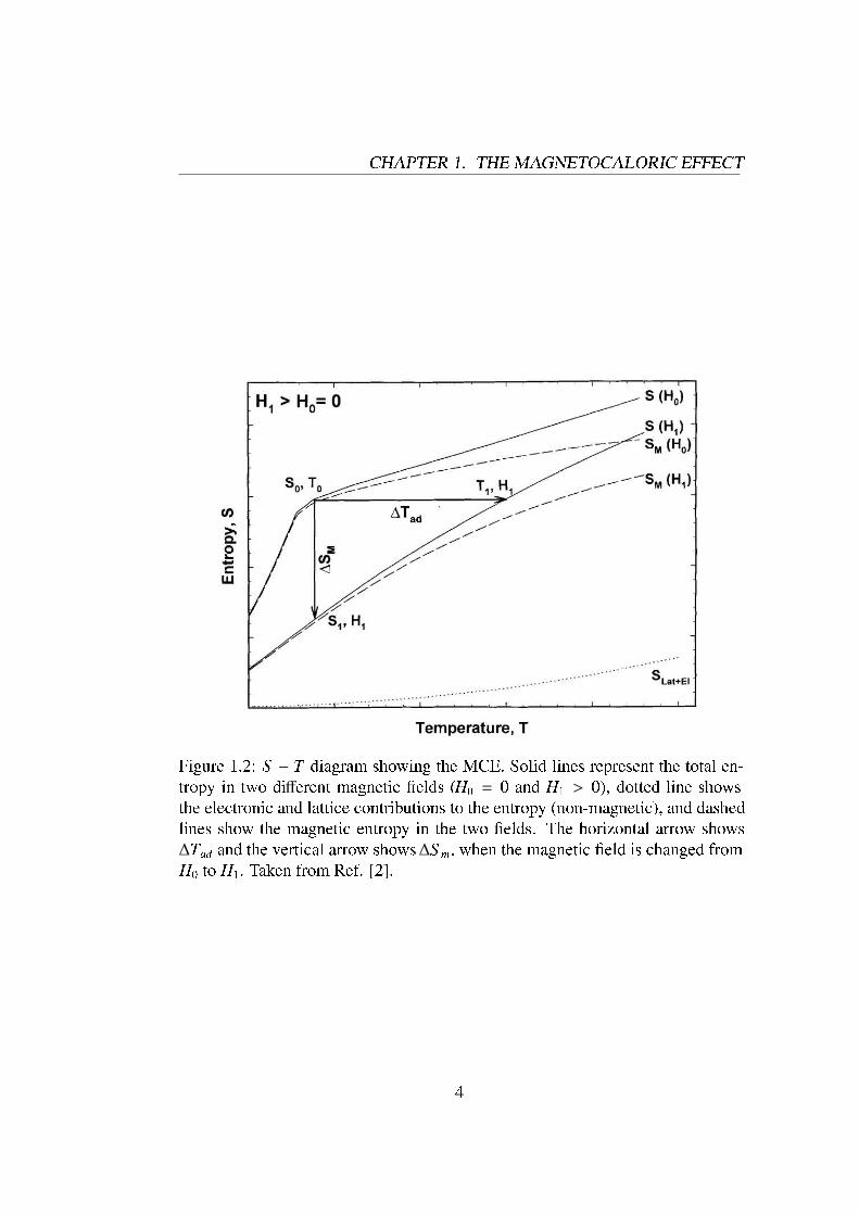
Figure 1.2: S − T diagram showing the MCE. Solid lines represent the total en-tropy in two different magnetic �elds (H0 = 0 and H1 > 0), dotted line showsthe electronic and lattice contributions to the entropy (non-magnetic), and dashedlines show the magnetic entropy in the two �elds. The horizontal arrow shows∆Tad and the vertical arrow shows ∆S m, when the magnetic �eld is changed fromH0 to H1. Taken from Ref. [2].

4

1.2. Basic theory

magnetic order decreases and∆Tad(T,−∆H) is thus negative, while ∆S m(T,−∆H)is positive, giving rise to a cooling of the magnetic solid.

The relation between H, the magnetisation of the material, M, and T , to theMCE values, ∆Tad(T,∆H) and ∆S m(T,∆H), is given by one of the Maxwell rela-tions [8], (

∂S (T,H)∂H

)

T=

(∂M(T,H)

∂T

)

H. (1.5)

Integrating Eq. 1.5 for an isothermal (and isobaric) process, we obtain

∆S m(T,∆H) =

∫ H2

H1

(∂M(T,H)

∂T

)

HdH . (1.6)

This equation indicates that the magnetic entropy change is proportional toboth the derivative of magnetisation with respect to temperature at constant �eldand to the �eld variation. Using the following thermodynamic relations [8]:

(∂T∂H

)

S= −

(∂S∂H

)

T

(∂T∂S

)

H(1.7)

CH = T(∂S∂T

)

H, (1.8)

where CH is the heat capacity at constant �eld, and taking into account Eq. 1.5,the in�nitesimal adiabatic temperature change is given by

dT )ad = −(

TC(T,H)

)

H

(∂M(T,H)

∂T

)

HdH . (1.9)

After integrating this equation, we obtain other expresion that characterisesthe magnetocaloric effect,

∆Tad(T,∆H) = −∫ H2

H1

(T

C(T,H)

)

H

(∂M(T,H)

∂T

)

HdH . (1.10)

By analysing Eqs. 1.6 and 1.10, some information about the behaviour of theMCE in solids can be gained:

1. Magnetisation at constant �eld in both paramagnets (PM) and simple FMsdecreases with increasing temperature, i.e., (∂M/∂T )H < 0. Hence ∆Tad(T,∆H)should be positive, while∆S m(T,∆H) should be negative for positive �eld changes,∆H > 0.

2. In FMs, the absolute value of the derivative of magnetisation with respect totemperature, |(∂M/∂T )H |, is maximum at TC, and therefore |∆S m(T,∆H)| shouldshow peak at T = TC.

5


3. Although it is not straightforward from Eq. 1.10 since the heat capacity atconstant �eld shows an anomalous behaviour nearTC, ∆Tad(T,∆H) in FMs showsa peak at the Curie temperature when∆H tends to zero [9].

4. For the same |∆S m(T,∆H)| value, the ∆Tad(T,∆H) value will be larger athigher T and lower heat capacity.

5. In PMs, the ∆Tad(T,∆H) value is only signi�cant at temperatures close toabsolute zero, since |(∂M/∂T )H | is otherwise small. Only when the heat capacityis also very small (same order as |(∂M/∂T )H |), can a relevant ∆Tad(T,∆H) valuebe obtained, which also happens only close to absolute zero. If we are interestedin sizeable ∆Tad(T,∆H) values at higher temperatures, we thus need a solid thatorders spontaneously.

1.3 Mesurement of the magnetocaloric effect1.3.1 Direct measurementsDirect techniques to measure MCE always involve the measurement of the initial(T0) and �nal (TF) temperatures of the sample, when the external magnetic �eldis changed from an initial (H0) to a �nal value (HF). Then the measurement of theadiabatic temperature change is simply given by

∆Tad(T0,HF − H0) = TF − T0 . (1.11)

Direct measurement techniques can be performed using contact and non-con-tact techniques, depending on whether the temperature sensor is directly con-nected to the sample or not.

To perform direct measurements of MCE, a rapid change of the magnetic �eldis needed. Therefore, the measurements can be carried out either on immobilisedsamples by changing the �eld [10] or by moving the sample in and out of a con-stant magnetic �eld region [11]. Using immobilised samples and pulsed mag-netic �elds, direct MCE measurements from 1 to 40 Tesla (T) have been reported.When electromagnets are used, the magnetic �eld is usually reduced to less than2 T. When the sample or the magnet are moved, permanent or superconductingmagnets are usually employed, with a magnetic �eld range of 0.1-10 T.

The accuracy of the direct experimental techniques depends on the errors inthermometry and in �eld setting, the quality of thermal insulation of the sample,the possible modi�cation of the reading of temperature sensor due to the applied�eld, etc. Considering all these effects, the accuracy is claimed to be within the5-10% range [2, 10, 11].

At this point, we must mention the new direct measurement of MCE associatedwith �rst-order �eld-induced magnetic phase transitions, that is presented in this

6

1.3. Mesurement of the magnetocaloric e�ect

thesis (see Chapter 4): a differential scanning calorimeter (DSC) operating underapplied magnetic �eld that measures the enthalpy of transformation (i.e., the latentheat) when the transition is induced by �eld. From the latent heat, the entropychange is obtained, being the �rst direct measurement of MCE performed throughthe entropy change.

1.3.2 Indirect measurementsUnlike direct measurements, which usually only yield the adiabatic temperaturechange, indirect experiments allow the calculation of both∆Tad(T,∆H) and ∆S m(T,∆H) in the case of heat capacity measurements, or just∆S m(T,∆H) in the case ofmagnetisation measurements. In the latter case, magnetisation must be measuredas a function of T and H. This allows to obtain ∆S m(T,∆H) by numerical inte-gration of Eq. 1.6, and it is very useful as a rapid search for potential magneticrefrigerant materials [12]. The accuracy of∆S m(T,∆H) calculated from magneti-sation data depends on the accuracy of the measurements of the magnetic moment,T and H. It is also affected by the fact that the exact differentials in Eq. 1.6 (dM,dH and dT ) are replaced by the measured variations (∆M, ∆T and ∆H). Takinginto account all these effects, the error in the value of ∆S m(T,∆H) lies within therange of 3-10% [2, 12].

The measurement of the heat capacity as a funcion of temperature in constantmagnetic �elds and pressure, C(T )P,H, provides the most complete characterisa-tion of MCE in magnetic materials. The entropy of a solid can be calculated fromthe heat capacity as:

S (T )H=0 =

∫ T

0

C(T )P,H=0

T dT + S 0

S (T )H,0 =

∫ T

0

C(T )P,H

T dT + S 0,H , (1.12)

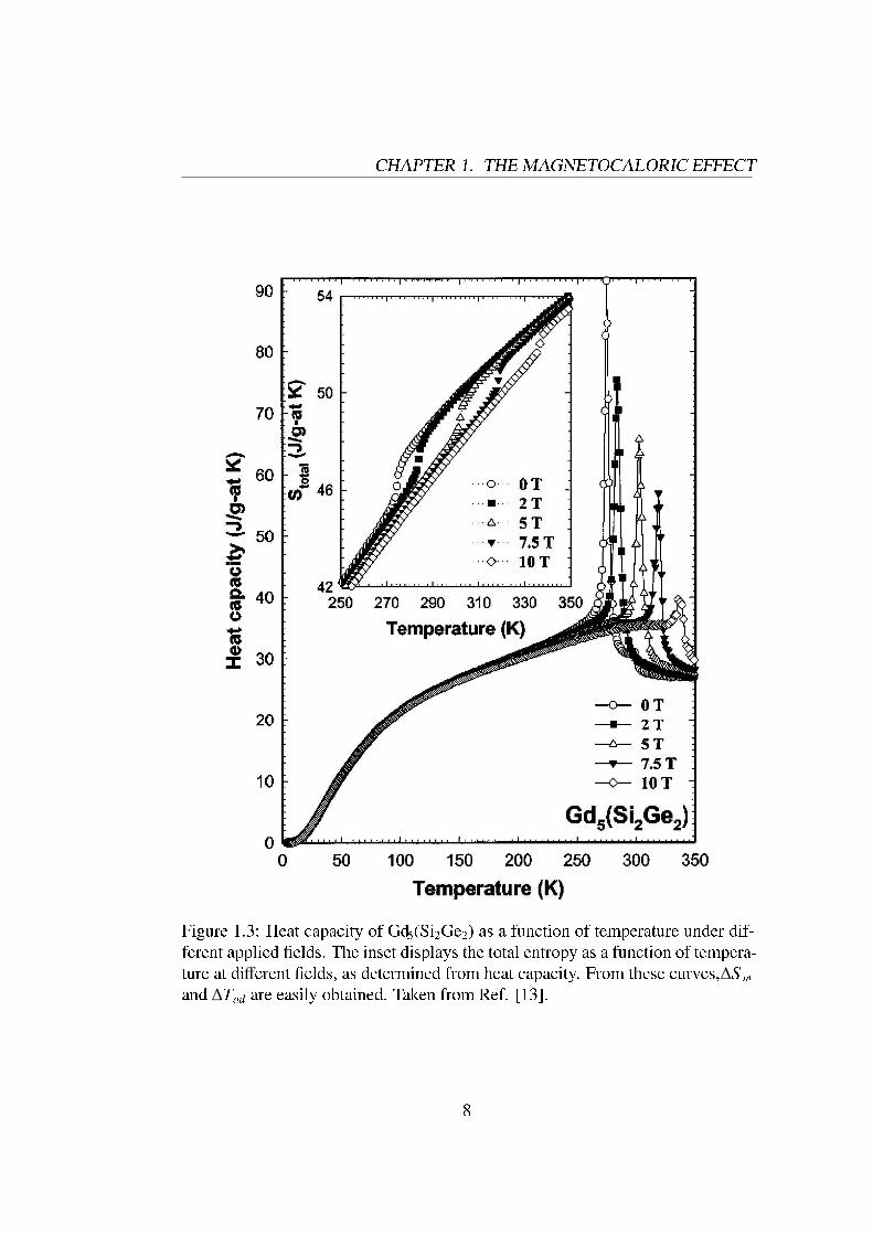
where S 0 and S 0,H are the zero temperature entropies. In a condensed systemS 0 = S 0,H [14]. Hence, if S (T )H is known, both ∆Tad(T,∆H) and ∆S m(T,∆H)can be obtained [15], see for example Fig. 1.3. However, this evaluation is notvalid if a �rst-order transition takes place within the evaluated range, since thevalue of CP is not de�ned at a �rst order transition (see Refs. [16, 17] and Chapter4). In this case, the entropy curves present a discontinuity, which corresponds tothe entropy change of the transition. The entropy discontinuity can be determinedfrom different experimental data, such as magnetisation or DSC, and then theresulting S (T )H functions can be corrected accordingly [16].

The accuracy in the measurements of MCE using heat capacity data dependscritically on the accuracy of C(T )P,H measurements and data processing, since

7


Figure 1.3: Heat capacity of Gd5(Si2Ge2) as a function of temperature under dif-ferent applied �elds. The inset displays the total entropy as a function of tempera-ture at different �elds, as determined from heat capacity. From these curves,∆S mand ∆Tad are easily obtained. Taken from Ref. [13].

8

1.4. Magnetocaloric e�ect in paramagnets

both ∆Tad(T,∆H) and ∆S m(T,∆H) are small differences between two large values(temperatures and total entropies). The error in ∆S m(T,∆H), σ[∆S m(T,∆H)],calculated from heat capacity is given by the expression [15]

σ[∆S m(T,∆H)] = σ[S (T,H = 0)] + σ[S (T,H , 0)] , (1.13)

whereσS (T,H = 0) and σS (T,H , 0) are the errors in the calculation of the zero�eld entropy and non-zero �eld entropy, respectively. The error in the value of theadiabatic temperature change, σ[∆Tad(T,∆H)], is also proportional to the errorsin the entropy, but it is inversely proportional to the derivative of the entropy withrespect to temperature [15]:

σ[∆Tad(T,∆H)] =σ[S (T,H = 0)](dS (T,H=0)

dT

) +σ[S (T,H , 0)](dS (T,H,0)

dT

) . (1.14)

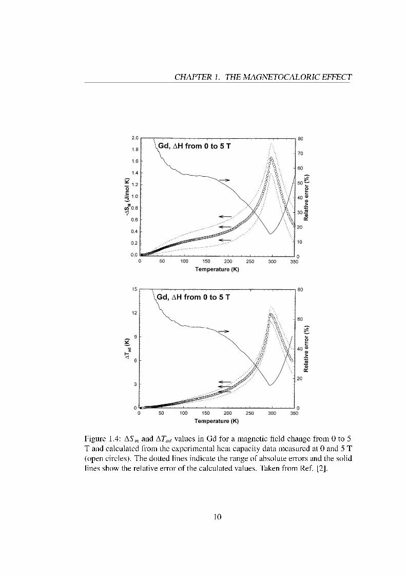
It is worth noting that Eqs. 1.13 and 1.14 yield the absolute error in MCEmeasurements and, therefore, the relative errors strongly increase for small MCEvalues (see Fig. 1.4). Assuming thus that the accuracy of the heat capacitymeasurements is not �eld dependent, the relative error in both∆Tad(T,∆H) and∆S m(T,∆H) is reduced for larger ∆H values.

1.4 Magnetocaloric effect in paramagnetsMCE in PMs was used as the �rst practical application, the so-called adiabatic de-magnetisation. With this technique, ultra-low temperatures can be reached (mK-µK). In 1927, the pioneering work of Giauque and MacDougall [5, 18] showedthat using the paramagnetic salt Gd2(SO4)3·8H2O, T lower than 1 K could bereached. Later, MCE at low temperatures was studied in other PM salts, suchas ferric ammonium alum [Fe(NH4)(SO4)·2H2O] [19], chromic potassium alum[20] and cerous magnesium nitrate [21]. The problem for the practical applicationof adiabatic demagnetisation using PM salts lies in its low thermal conductivity.Hence, the next step was the study of PM intermetallic compounds. One of themost studied materials was PrNi5 and it is actually still used in nuclear adiabaticdemagnetisation devices. Using PrNi5 the lowest working temperature has beenreached: 27 µK [22]. Another group of materials that have extensively been stud-ied are PM garnets, because of their high thermal conductivity, low lattice heatcapacity and very low ordering temperature (usually below 1 K). An orderingtemperature so close to absolute zero allows to obtain a large∆S m and to keepa signi�cant MCE up to ∼20K. For instance, ∆Tad within 6 and 10 K have beenreached in ytterbium (Y3Fe5O12) and gadolinium (Gd3Fe5O12) iron garnets, withµ0∆H = 11 T, in the 10-30 K T -range [23]. Appreciable MCE values have also

9


Figure 1.4: ∆S m and ∆Tad values in Gd for a magnetic �eld change from 0 to 5T and calculated from the experimental heat capacity data measured at 0 and 5 T(open circles). The dotted lines indicate the range of absolute errors and the solidlines show the relative error of the calculated values. Taken from Ref. [2].

10

1.5. MCE in order-disorder magnetic phase transitions

been reached using neodymium gallium garnet (Nd3Ga5O12) at 4.2 K [24] andgadolinium gallium garnet (Gd3Ga5O12) below 15 K [25]. Finally, a large value of∆S m has been observed in magnetic nanocomposites based on the iron-substitutedgadolinium gallium garnets, Gd3Ga5−xFexO12, for x ≤ 2.5 [26].

1.5 MCE in order-disorder magnetic phase transi-tions

Spontaneous magnetic ordering of PM solids below a given temperature is a co-operative phenomenon. The ordering temperature depends on the strenght of ex-change interaction and on the nature of the magnetic sublattice in the material.When spontaneous magnetic ordering occurs, the magnetisation strongly variesin a very narrow temperature range in the vicinity of the transition temperature,i.e., the Néel temperature for antiferromagnets (AFMs) and the Curie temperaturefor FMs. The fact that |(∂M/∂T )H | is large allows these magnetic materials tohave a signi�cant MCE. Since it is not the absolute value of the magnetisation,but rather its derivative with respect to temperature the one that must be large toobtain a large MCE, rare-earth metals or lanthanides (4 f metals) and their alloyshave been studied much more extensively than 3d transition metals and their al-loys, because the available magnetic entropy in rare earths is considerably largerthan in 3d transition metals: the maximum magnetic entropy for a lanthanide isS m = R ln(2J + 1), where R is the universal gas constant and J is the total angularmomentum.

The MCE in the vicinity of an order-disorder magnetic phase transition iscalculated by using equations 1.6 and 1.10, which arise from the Maxwell relation(Eq. 1.5), since these transitions are second-order and thermodynamic variableschange continuously [1, 17]. The research on these type of materials has beencentered in soft FMs with TC between 4 and 77 K, suitable for applications suchas for example helium and nitrogen liquefaction, and also in materials which ordernear room temperature so as to use their magnetocaloric properties in magneticrefrigeration and air conditioning.

1.5.1 MCE in the low-temperature range (∼10-80 K)The �rst evident choise for low-temperature magnetic refrigerant materials aresome pure rare earths such as Nd, Er and Tm, since they order at low tempera-tures. Anyway, the expectations for large MCE are not ful�lled. MCE in Nd reach∆Tad ∼ 2.5 K at T=10 K for a magnetic �eld rise µ0∆H = 10 T [27]. The prob-lem in Er is that several magnetic phase transitions occur between 20 and 80 K,

11


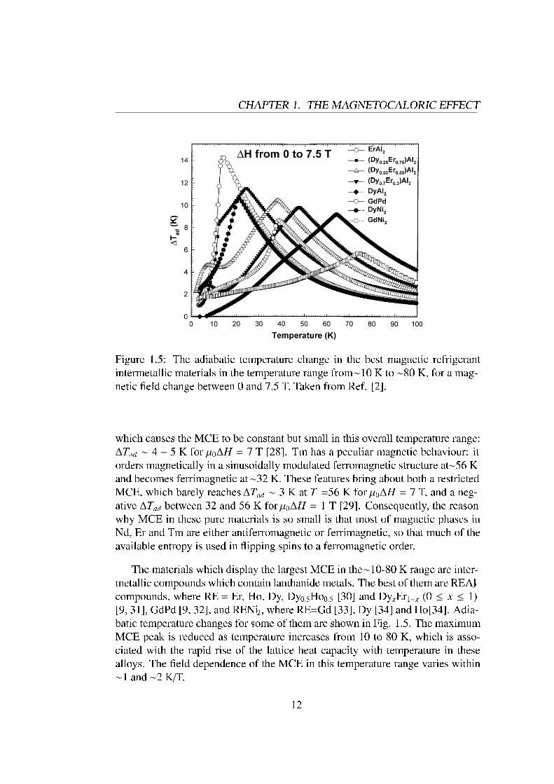
Figure 1.5: The adiabatic temperature change in the best magnetic refrigerantintermetallic materials in the temperature range from∼10 K to ∼80 K, for a mag-netic �eld change between 0 and 7.5 T. Taken from Ref. [2].

which causes the MCE to be constant but small in this overall temperature range:∆Tad ∼ 4 − 5 K for µ0∆H = 7 T [28]. Tm has a peculiar magnetic behaviour: itorders magnetically in a sinusoidally modulated ferromagnetic structure at∼56 Kand becomes ferrimagnetic at∼32 K. These features bring about both a restrictedMCE, which barely reaches ∆Tad ∼ 3 K at T =56 K for µ0∆H = 7 T, and a neg-ative ∆Tad between 32 and 56 K for µ0∆H = 1 T [29]. Consequently, the reasonwhy MCE in these pure materials is so small is that most of magnetic phases inNd, Er and Tm are either antiferromagnetic or ferrimagnetic, so that much of theavailable entropy is used in �ipping spins to a ferromagnetic order.

The materials which display the largest MCE in the∼10-80 K range are inter-metallic compounds which contain lanthanide metals. The best of them are REAl2compounds, where RE = Er, Ho, Dy, Dy0.5Ho0.5 [30] and DyxEr1−x (0 ≤ x ≤ 1)[9, 31], GdPd [9, 32], and RENi2, where RE=Gd [33], Dy [34] and Ho[34]. Adia-batic temperature changes for some of them are shown in Fig. 1.5. The maximumMCE peak is reduced as temperature increases from 10 to 80 K, which is asso-ciated with the rapid rise of the lattice heat capacity with temperature in thesealloys. The �eld dependence of the MCE in this temperature range varies within∼1 and ∼2 K/T.

12

1.5. MCE in order-disorder magnetic phase transitions

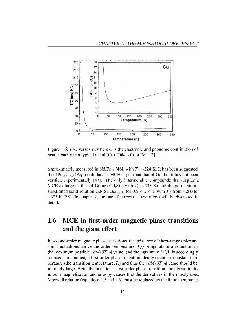
1.5.2 MCE in the intermediate-temperature range (∼80-250 K)This temperature range has not been much studied, mainly for two reasons. First,there are not many applications in this range (it lies above gas liquefactions andbelow room temperature). Second, theT/C fraction (where C is the phononic andelectronic contribution to heat capacity) presents an inherent minimum in metals,as shown in �gure 1.6 for a typical metal (Cu). This suggests that the adiabatictemperature variation is minimal in this temperature range (see equations 1.9 and1.10).

One of the best magnetic refrigerant materials in this temperature range ispure Dy [9, 35], with ∆Tad ∼ 12 K at T ∼180 K for a magnetic �eld changeµ0∆H = 7 T. As discussed earlier for Tm (section 1.5.1), Dy also presents complexmagnetic structures, which brings about a negative MCE for small �eld changes(µ0∆H < 2 T). Recent works [36, 37] have also found a noticeable MCE in amor-phous REx(T1,T2)1−x alloys, where RE is a rare earth metal and T1, T2 are 3dtransition metals, in the range 100-200 K. The �eld dependence of the MCE is2 K/T for Dy, but for the rest of the materials, such as those amorphous alloys,rarely reaches 1 K/T. In spite of all these difficulties for the MCE at the interme-diate temperatures, the recently discovered Gd5(SixGe1−x)4 alloys show extremelylarge ∆S m and ∆Tad values, from 2 to 10 times larger than any of the above men-tioned materials [38, 39]. We will later discuss on these alloys, since they are alsoforeseen as excellent magnetic re�gerant materials at room temperature (see sec-tion 1.5.3). The origin of this giant MCE is explained in section 1.6, while theirproperties are exhaustively discussed in chapter 2.

1.5.3 MCE near room temperatureThe prototype material at room temperature is Gd, a rare earth metal which ordersFM at TC=294 K. This lanthanide has been extensively studied [9, 10, 40, 41], and∆Tad values at TC are ∼6, 12, 16 and 20 K for magnetic �eld changesµ0∆H = 2,5, 7.5 and 10 T, respetively, leading to a �eld dependence of the MCE of∼3 K/Tat low �elds, which reduces to∼2 K/T at higher �elds. A variety of alloys usingGd and other rare earths have been prepared in order to improve the MCE in Gd.Gd-RE alloys, with RE=lanthanide (Tb, Dy, Er, Ho,...) [42, 43] and/or Y [44]have been studied, but the alloying only decreases TC - which is not desirable,since we depart from room temperature - while the MCE value does not increaseconsiderably with respect to pure Gd. The only exceptions are nanocrystalline Gd-Y alloys, which improve the MCE in Gd forµ0∆H = 1 T [45]. Most intermetalliccompounds that order magnetically near room temperature and above∼290 Kshow a noticeble lower MCE than that of Gd. For example Y2Fe17, with TC ∼310K, yields a MCE which is about 50% of that in Gd [46]. The same magnitude is

13


Figure 1.6: T/C versus T , where C is the electronic and phononic contribution ofheat capacity in a typical metal (Cu). Taken from Ref. [2].

approximately measured in Nd2Fe17 [46], with TC ∼324 K. It has been suggestedthat (Pr1.5Ce0.5)Fe17 could have a MCE larger than that of Gd, but it has not beenveri�ed experimentally [47]. The only intermetallic compounds that display aMCE as large as that of Gd are Gd5Si4 (with TC ∼335 K) and the germanium-substituted solid solution Gd5(SixGe1−x)4, for 0.5 ≤ x ≤ 1, with TC from ∼290 to∼335 K [38]. In chapter 2, the main features of these alloys will be discussed indetail.

1.6 MCE in �rst-order magnetic phase transitionsand the giant effect

In second-order magnetic phase transitions, the existence of short-range order andspin �uctuations above the order temperature (TC) brings about a reduction inthe maximum possible |(∂M/∂T )H | value, and the maximum MCE is accordinglyreduced. In contrast, a �rst-order phase transition ideally occurs at constant tem-perature (the transition temperature, Tt) and thus the |(∂M/∂T )H | value should bein�nitely large. Actually, in an ideal �rst-order phase transition, the discontinuityin both magnetisation and entropy causes that the derivatives in the mostly usedMaxwell relation (equations 1.5 and 1.6) must be replaced by the �nite increments

14

1.6. MCE in �rst-order magnetic phase transitions and the giant e�ect

of the Clausius-Clapeyron equation for phase transformations. The discontinuityin the entropy is related to the entalphy of transformation, which is also calledlatent heat. The �rst-order transition occurs if the two magnetic phases have equalthermodynamic potential [48, 49],[U1 −

n1M21

2

]−ΘS 1+(pV1−HM1) =

[U2 −

n2M22

2

]−ΘS 2+(pV2−HM2) , (1.15)

where Θ is the transition temperature at the �eld H, and U1,2, S 1,2, V1,2, M1,2 arethe internal energy, entropy, volume and magnetisation of phases 1 and 2, andnM2

describes the molecular �eld contribution. If we assume that the external �eld onlytriggers the transition, but does not change the value of the physical parameters(S , M, V, n) in either phase, the difference of the transition temperature for a �eldchange of ∆H is given as

∆Θ

∆H = −∆M∆S = const , (1.16)

where ∆M = M2 − M1 is the difference between the magnetisations and ∆S =

S 2 − S 1 the difference between the entropies of the two phases. The sign appearssince a magnetised phase has lower entropy. ∆Θ/∆H is the shift of the transitiontemperature with the transition �eld, which is usually evaluated asdTt/dHt froma Tt(Ht) curve. Therefore, the Clausius-Clapyron equation is written as

∆S = −∆M dHt

dTt. (1.17)

Chapter 5 discusses extensively the use of the Clausius-Clapeyron equation. Theexistence of this entropy change associated with the �rst-order transition bringsabout an extra contribution to MCE, yielding the so-called giant magnetocaloriceffect. The use of this entropy change can be possible provided that the phasetransition -and thus the entropy change- is induced by magnetic �eld. Extensivelysearch for materials with a �rst-order �eld-induced magnetic phase transition haslately been shown in literature.

The intermetallic compound FeRh was one of the �rst materials in which thistype of giant (and negative) MCE was observed. This alloy has a �rst-order FM-to-AFM phase transition at Tt ∼316 K, which yields a MCE value as large as -8.4K for µ0∆H = 2.1 T [50]. Unfortunately the giant effect is irreversible, and giantMCE can only be observed in virgin samples.

The recently discovered Gd5(SixGe1−x)4 alloys with 0 ≤ x ≤ 0.5, display a∆S m at least twice larger than that of Gd near room temperature (-18.5 J/(kgK)for µ0∆H = 5 T at T= 276 K) [13], and between 2 and 10 times larger than thebest magnetocaloric materials in the low and intermediate temperature ranges (-26 J/(kgK) at T ∼40 K to -68 J/(kgK) at T ∼145 K for µ0∆H = 5 T, depending

15


on composition, x) [38]. ∆Tad is also very large, reaching for example 15.2 K forµ0∆H = 5 T at T= 276 K and 15 K forµ0∆H = 5 T at T ∼ 70 K [39]. These alloyshave some interesting properties that make them very exciting and candidates tobe used as magnetic refrigerant materials in highly efficient magnetic refrigerators.The �rst one is that the transition temperature can be tuned from∼20 K to ∼276K by just changing the ratio between Si and Ge contents (0 ≤ x ≤ 0.5) [38, 51],and even a Tt ∼305 K can be achieved by adding Ga impurities to Gd5(Si2Ge2)[52]. This allows one to shift at own's will the maximum giant MCE between∼20 and ∼305 K. The second property is that, unlike FeRh, Gd5(SixGe1−x)4 alloysshow a reversible MCE, i.e., MCE does not disappear after the �rst applicationof a magnetic �eld. The difference in the behaviour of FeRh and Gd5(SixGe1−x)4alloys is associated with the nature of the �rst-order phase transition: while theformer has a magnetic order-order transition, the latter plays simultaneously acrystallographic order-order phase transition and a magnetic phase transition, thelatter being order-disorder for 0.24 ≤ x ≤ 0.5 and order-order for 0 ≤ x ≤ 0.2[51, 53, 54, 55]. This magnetoelastic coupling accounts for the rare existence ofa �rst-order magnetic order-disorder phase transition and also for the �rst-ordermagnetic order-order phase transition. This is exhaustively developed in Chapter2.

Following the outburst caused by the discovery of a giant MCE in Gd5(SixGe1−x)4 intermetallic alloys, extensive research is being undertaken to �nd newintermetallic alloys showing �rst-order �eld-induced phase transitions, which isgenerally associated with a strong magnetoelastic coupling. The �rst obvious stephas been to exchange Gd for other rare earth cation in RE5(SixGe1−x)4 alloys, withRE=lanthanide [56]. Some of them, such as for example RE=Tb, seem to showmagnetoelastic similar properties to that of Gd5(SixGe1−x)4, yielding a noticeableMCE (∼ -22 J/(kgK) for µ0∆H=5 T at Tt ∼110 K) [57]. Dy5(SixGe1−x)4 alsoshows a �rst-order phase transition for 0.67 ≤ x ≤ 0.78, which yields a MCE of∼ -34 J/(kgK) for µ0∆H=5 T at Tt ∼65 K [58]. The study of the actual mechanismresponsible for the giant MCE in RE5(SixGe1−x)4 alloys makes them interesting,but the low temperature transition that show most of these alloys makes them un-suitable from the point of view of applications near room temperature, in contrastto Gd5(SixGe1−x)4.

MnAs is also well-known for its �rst-order magnetoelastic phase transitionfrom FM (with NiAs-type hexagonal crystallographic structure) to PM (with MnP-type orthorhombic structure) order at Tt=318 K, and it might also be a good can-didate since it shows giant MCE (-30 J/(kgK) and 13 K for µ0∆H=5 T at Tt).Unfortunately, it is not very useful for applications due to its large thermal hys-teresis at the transition [59]. However, the partial substitution of As by Sb inMn(AsxSb1−x) reduces both the thermal hysteresis and the transition temperature,which decreases from 318 K for x=0 to 230 K for x=0.3, maintaining �rst-order

16

1.6. MCE in �rst-order magnetic phase transitions and the giant e�ect

Figure 1.7: Entropy changes of MnFeP0.45As0.55 (solid circles), Gd5(Si2Ge2) (in-verted solid triangles) and Gd (solid triangles). Data are shown for external �eldvariations of 0-2 T (lower curves for each material), and 0-5 T (upper curves),calculated from magnetisation measurements. Taken from Ref. [63].

and magnetoelastic properties. Hence, a competitive material in a wide temper-ature range around room temperature is obtained (-25 to -30 J/(kgK) and ∼10 Kfor µ0∆H=5 T) [59, 60]. Moreover, the addition of Fe and P in the MnFePxAs1−xalloys still maintains the �rst-order and �eld-induced nature of the phase transi-tion near room temperature, for 0.26≤ x ≤0.66 [61, 62]. For example, x=0.45yields -18 J/(kgK) for µ0∆H=5 T at Tt ∼300 K [63]. A comparison of the entropychange of MnFeP0.45As0.55 to those of Gd5(Si2Ge2) and pure Gd is given in Fig.1.7. The advantage in these alloys is that they are transition-metal-based, whichare much cheaper than rare earths, and the disadvantage is the poissonousness ofthe As content [64].

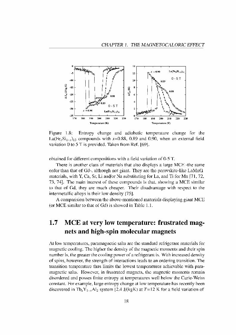
Finally, it has recently been found that the La(FexSi1−x)13 series of alloys alsoshows a �rst-order �eld-induced FM-PM transition within x=0.86 (Tt ∼210 K)and x=0.90 (Tt ∼184 K) [65, 66]. However, an itinerant electron metamagnetictransition takes place in this case [66]. That brings about a giant MCE, withan entropy change from -14 to -28 J/(kgK) and a ∆Tad between 6 and 8 K, forµ0∆H=2 T [67, 68, 69]. In order to increase Tt up to room temperature, either Cocan be added [70] or hydrogen can be absorbed [68, 69], maintaining the gianteffect. Figure 1.8 shows the entropy change and the adiabatic temperature change

17


0 - 5 T

0 - 5 T

Figure 1.8: Entropy change and adiabatic temperature change for theLa(FexSi1−x)13 compounds with x=0.88, 0.89 and 0.90, when an external �eldvariation 0 to 5 T is provided. Taken from Ref. [69].

obtained for different compositions with a �eld variation of 0-5 T.There is another class of materials that also displays a large MCE -the same

order than that of Gd-, although not giant. They are the perovskite-like LaMnO3materials, with Y, Ca, Sr, Li and/or Na substituting for La, and Ti for Mn [71, 72,73, 74]. The main interest of these compounds is that, showing a MCE similarto that of Gd, they are much cheaper. Their disadvantage with respect to theintermetallic alloys is their low density [75].

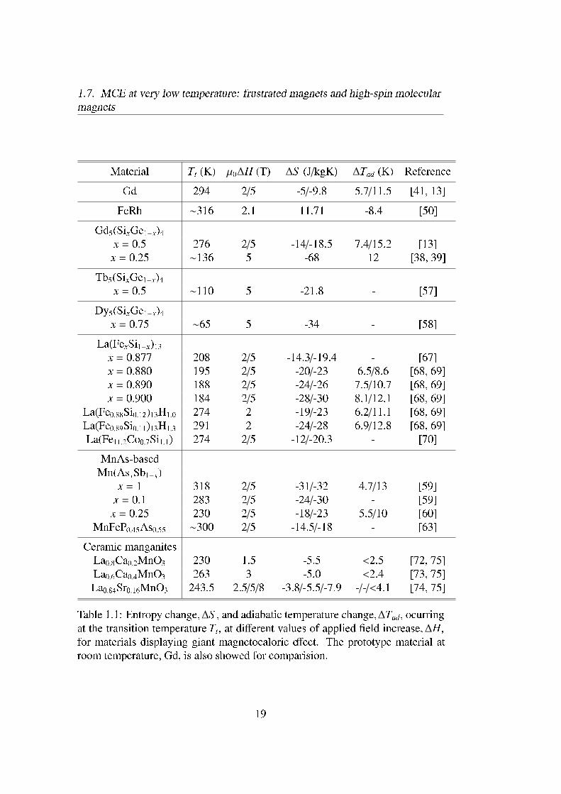
A comparision between the above-mentioned materials displaying giant MCE(or MCE similar to that of Gd) is showed in Table 1.1.

1.7 MCE at very low temperature: frustrated mag-nets and high-spin molecular magnets

At low temperatures, paramagnetic salts are the standard refrigerant materials formagnetic cooling. The higher the density of the magnetic moments and their spinnumber is, the greater the cooling power of a refrigerant is. With increased densityof spins, however, the strength of interactions leads to an ordering transition. Thetransition temperature thus limits the lowest temperatures achievable with para-magnetic salts. However, in frustrated magnets, the magnetic moments remaindisordered and posses �nite entropy at temperatures well below the Curie-Weissconstant. For example, large entropy change at low temperature has recently beendiscovered in TbxY1−xAl2 system [2.4 J/(kgK) at T=12 K for a �eld variation of

18

1.7. MCE at very low temperature: frustrated magnets and high-spin molecularmagnets

Material Tt (K) µ0∆H (T) ∆S (J/kgK) ∆Tad (K) ReferenceGd 294 2/5 -5/-9.8 5.7/11.5 [41, 13]

FeRh ∼316 2.1 11.71 -8.4 [50]Gd5(SixGe1−x)4

x = 0.5 276 2/5 -14/-18.5 7.4/15.2 [13]x = 0.25 ∼136 5 -68 12 [38, 39]

Tb5(SixGe1−x)4x = 0.5 ∼110 5 -21.8 - [57]

Dy5(SixGe1−x)4x = 0.75 ∼65 5 -34 - [58]

La(FexSi1−x)13x = 0.877 208 2/5 -14.3/-19.4 - [67]x = 0.880 195 2/5 -20/-23 6.5/8.6 [68, 69]x = 0.890 188 2/5 -24/-26 7.5/10.7 [68, 69]x = 0.900 184 2/5 -28/-30 8.1/12.1 [68, 69]

La(Fe0.88Si0.12)13H1.0 274 2 -19/-23 6.2/11.1 [68, 69]La(Fe0.89Si0.11)13H1.3 291 2 -24/-28 6.9/12.8 [68, 69]La(Fe11.2Co0.7Si1.1) 274 2/5 -12/-20.3 - [70]

MnAs-basedMn(AsxSb1−x)

x = 1 318 2/5 -31/-32 4.7/13 [59]x = 0.1 283 2/5 -24/-30 - [59]x = 0.25 230 2/5 -18/-23 5.5/10 [60]

MnFeP0.45As0.55 ∼300 2/5 -14.5/-18 - [63]Ceramic manganites

La0.8Ca0.2MnO3 230 1.5 -5.5 <2.5 [72, 75]La0.6Ca0.4MnO3 263 3 -5.0 <2.4 [73, 75]La0.84Sr0.16MnO3 243.5 2.5/5/8 -3.8/-5.5/-7.9 -/-/<4.1 [74, 75]

Table 1.1: Entropy change, ∆S , and adiabatic temperature change,∆Tad, ocurringat the transition temperature Tt, at different values of applied �eld increase, ∆H,for materials displaying giant magnetocaloric effect. The prototype material atroom temperature, Gd, is also showed for comparision.

19


µ0∆H=2 T and 7.6 J/(kgK) at T=30 K for µ0∆H=2 T], associated with the spin-glass-to-PM (freezing) transition [76]. Moreover, enhanced magnetocaloric effecthas been predicted in geometrically frustrated magnets [77]. This enhancementis related to the presence of a macroscopic number of soft modes associated withgeometrical frustration below the saturation �eld.

Another interesting type of materials showing large (and time-dependent) en-tropy change at very low temperature are the high-spin molecular magnets. Molec-ular clusters as Mn12 and Fe8 exhibit extremely high entropy change around theblocking temperature at the Kelvin regime, which is associated with the order-disorder blocking process. Values of 21 J/(kgK) at T '3 K for a �eld variation ofµ0∆H=3 T at a sweeping rate of 0.01 Hz are obtained for Mn12 [78]. Therefore,they are potential candidates to magnetic refrigerants in the helium liquefactionregime.

1.8 Magnetic refrigerationCurrently, there is a great deal of interest in utilizing the MCE as an alternatetechnology for refrigeration both in the ambient temperature and in cryogenictemperatures. Magnetic refrigeration is an environmentally friendly cooling tech-nology (see Fig. 1.9 for details). It does not use ozone-depleting chemicals (suchas chloro�uorocarbons), hazardous chemicals (such as ammonia), or greenhousegases (hydrochloro�uorocarbons and hydro�uorocarbons). Most modern refrig-eration systems and air conditioners still use ozone-depleting or global-warmingvolatile liquid refrigerants. Magnetic refrigerators use a solid refrigerant (usuallyin a form of spheres or thin sheets) and common heat transfer �uids (e.g. water,water-alcohol solution, air, or helium gas) with no ozone-depleting and/or global-warming effects. Another important difference between vapour-cycle refrigera-tors and magnetic refrigerators is the amount of energy loss incurred during therefrigeration cycle. Even the newest most efficient commercial refrigeration unitsoperate well below the maximum theoretical (Carnot) efficiency, and few, if any,further improvements may be possible with the existing vapor-cycle technology.Magnetic refrigeration, however, is rapidly becoming competitive with conven-tional gas compression technology because it offers considerable operating costsavings by eliminating the most inefficient part of the refrigerator: the compres-sor. The cooling efficiency of magnetic refrigerators working with Gd has beenshown [2, 6, 7, 79] to reach 60% of the Carnot limit, compared to only about 40%in the best gas-compression refrigerators. However, with the currently availablemagnetic materials, this high efficiency is only realised in high magnetic �eldsof 5 T. Therefore, research for new magnetic materials displaying larger MCE,which then can be operated in lower �elds of about 2 T that can be generated by

20

1.8. Magnetic refrigeration

Figure 1.9: Schematic representation of a magnetic-refrigeration cycle, whichtransports heat from the heat load to its surroundings. Light and dark grey de-pict the magnetic material without and with applied magnetic �eld, respectively.Initially disordered magnetic moments are aligned by a magnetic �eld, resultingin heating of the magnetic material. This heat is removed from the material toits surroundings by a heat-transfer medium. On removing the �eld, the magneticmoments randomize, which leads to cooling of the magnetic material below theambient temperature. Heat from the system to be cooled can then be extractedusing a heat-transfer medium. Taken from Ref. [63].

21


permanent magnets, is very signi�cant. The heating and cooling that occurs in themagnetic refrigeration technique is proportional to the size of the magnetic mo-ments and to the applied magnetic �eld. This is why research in magnetic refrig-eration is at present almost exclusively conducted on superparamagnetic materialsand on rare-earth compounds.

Refrigeration in the subroom temperature (∼250-290 K) range is of partic-ular interest because of potential impact on energy savings and environmentalconcerns. As described along this chapter, materials to be applied in magneticrefrigeration must present a series of properties:

(i) A �rst-order �eld-induced transition around the working temperature, inorder to utilise the associated entropy change.

(ii) A high refrigerant capacity. Refrigerant capacity,q, is a measure of howmuch heat can be transferred between the cold and hot sinks in one ideal refriger-ation cycle, and it is calculated as:

q =

∫ Thot

Tcold

∆S (T )∆H dT . (1.18)

Therefore, a large entropy change in a temperature range as wide as possibleis needed. Moreover, it is easy to argue that for any practical application it isthe amount of heat energy per unit volume transferred in one refrigeration cycle,which is the important parameter, i.e., the denser the magnetic refrigerant the moreeffective it is [75].

(iii) A low magnetic hysteresis, to avoid magnetic-work losses due to the ro-tation of domains in a magnetic-refrigeration cycle.

(iv) A low heat capacity CP, since a high CP increases the thermal load andmore energy is required to heat the sample itself and causes a loss in entropy,i.e.for a given ∆S , ∆Tad will be lower.

(v) Low cost and harmless. The main problem of the rare-earth-based com-pounds, which are usually the best magnetic refrigerants in the whole temperaturerange (including pure Gd at room temperature) is their high cost. 3d-transition-metal compounds or ceramic manganites are a good alternative concerning thecost of the materials. In particular, the recently reported MnAs-based materialsshow good prospects [59, 63]. However, the presence of As in these compounds,which is poisonous, could make them be useless for commercial applications.Another type of compounds, La(FexSi1−x)13, also presents a large MCE at roomtemperature, has a low cost and in this case all elements are harmless [68, 69].

22

Bibliography

Bibliography[1] A. M. Tishin, in Handbook of Magnetic Materials, edited by K. H. J.

Buschow (North Holland, Amsterdam, 1999), Vol. 12, pp. 395�524.

[2] V. K. Pecharsky and K. A. Gschneidner, Jr., J. Magn. Magn. Mater.200, 44(1999).

[3] E. Warburg, Ann. Phys. 13, 141 (1881).

[4] P. Debye, Ann. Phys. 81, 1154 (1926).

[5] W. F. Giauque, J. Amer. Chem. Soc.49, 1864 (1927).

[6] V. K. Pecharsky and K. A. Gschneidner, Jr., J. Appl. Phys.85, 5365 (1999).

[7] K. A. Gschneidner, Jr. and V. K. Pecharsky, Annu. Rev. Mater. Sci.30, 387(2000).

[8] A. H. Morrish, The Physical Principles of Magnetism (Wiley, New York,1965), Chap. 3.

[9] A. M. Tishin, K. A. Gschneidner, Jr., and V. K. Pecharsky, Phys. Rev. B59,503 (1999).

[10] S. Y. Dan'kov, A. M. Tishin, V. K. Pecharsky, and K. A. Gschneidner, Jr.,Rev. Sci. Instrum. 68, 2432 (1997).

[11] B. R. Gopal, R. Chahine, and T. K. Bose, Rev. Sci. Instrum.68, 1818 (1997).

[12] M. Földeàki, R. Chahine, and T. K. Bose, J. Appl. Phys.77, 3528 (1995).

[13] V. K. Pecharsky and K. A. Gschneidner, Jr., Phys. Rev. Lett.78, 4494 (1997).

[14] M. W. Zemansky, Heat and Thermodynamics, 6th ed. (McGraw-Hill, NewYork, 1981).

[15] V. K. Pecharsky and K. A. Gschneidner, Jr., Adv. Cryog. Eng. 42A, 423(1996).


[17] V. K. Pecharsky, K. A. Gschneidner, Jr., A. O. Pecharsky, and A. M. Tishin,Phys. Rev. B 64, 144406 (2001).

[18] W. F. Giauque and I. P. D. McDougall, Phys. Rev.43, 768 (1933).

23


[19] A. H. Cooke, Proc. Roy. Soc. A 62, 269 (1949).

[20] B. Bleaney, Proc. Roy. Soc. A 204, 203 (1950).

[21] A. H. Cooke, H. J. Duffus, and W. P. Wolf, Philos. Mag. 44, 623 (1953).

[22] H. Ishimoto, N. Nishida, T. Furubayashi, M. Shinohara, Y. Takano, Y. Miura,and K. Ono, J. Low Temp. Phys. 55, 17 (1984).

[23] A. E. Clark and R. S. Alben, J. Appl. Phys.41, 1195 (1970).

[24] V. Nekvasil, V. Roskovec, F. Zounova, and P. Novotny, Czech. J. Phys.24,810 (1974).

[25] R. Z. Levitin, V. V. Snegirev, A. V. Kopylov, A. S. Lagutin, and A. Gerber,J. Magn. Magn. Mat. 170, 223 (1997).

[26] R. D. Shull, R. D. McMichael, and J. J. Ritter, Nanostruct. Mater.2, 205(1993).

[27] C. B. Zimm, P. M. Ratzmann, J. A. Barclay, G. F. Green, and J. N. Chafe,Adv. Cryog. Eng. 36, 763 (1990).

[28] C. B. Zimm, P. L. Kral, J. A. Barclay, G. F. Green, and W. G. Patton, inPro-ceedings of the 5th International Cryocooler Conference(Wright Researchand Development Center, Wright Patterson Air Force base, Ohio, 1988), p.49.

[29] C. B. Zimm, J. A. Barclay, H. H. Harkness, G. F. Green, and W. G. Patton,Cryogenics 29, 937 (1989).

[30] T. Hashimoto, T. Kuzuhara, M. Sahashi, K. Inomata, A. Tomokiyo, and H.Yayama, J. Appl. Phys. 62, 3873 (1987).

[31] H. Takeya, V. K. Pecharsky, K. A. Gschneidner, Jr., and J. O. Moorman,Appl. Phys. Lett. 64, 2739 (1994).

[32] J. A. Barclay, W. C. Overton, and C. B. Zimm, inLT-17 Contributed Papers,edited by U. Ekren, A. Schmid, W. Weber, and H. Wuhl (Elsevier Science,Amsterdam, 1984), p. 157.

[33] C. B. Zimm, E. M. Ludeman, M. C. Serverson, and T. A. Henning, Adv.Cryog. Eng. 37B, 883 (1992).

[34] A. Tomokiyo, H. Yayama, H. Wakabayashi, T. Kuzuhara, T. Hashimoto, M.Sahashi, and K. Inomata, Adv. Cryog. Eng.32, 295 (1986).

24

Bibliography

[35] S. M. Benford, J. Appl. Phys. 50, 1868 (1979).

[36] X. Y. Liu, J. A. Barclay, M. Földeàki, B. R. Gopal, R. Chahine, and T. K.Bose, Adv. Cryog. Eng. 42A, 431 (1997).

[37] M. Földeàki, R. Chahine, B. R. Gopal, T. K. Bose, X. Y. Liu, and J. A.Barclay, J. Appl. Phys. 83, 2727 (1998).

[38] V. K. Pecharsky and K. A. Gschneidner, Jr., Appl. Phys. Lett. 70, 3299(1997).

[39] V. K. Pecharsky and K. A. Gschneidner, Jr., Adv. Cryog. Eng. 43, 1729(1998).

[40] S. M. Benford and G. Brown, J. Appl. Phys.52, 2110 (1981).

[41] S. Y. Dan'kov, A. M. Tishin, V. K. Pecharsky, and K. A. Gschneidner, Jr.,Phys. Rev. B 57, 3478 (1998).

[42] S. A. Nikitin, A. S. Andreenko, A. M. Tishin, A. M. Arkharov, and A. A.Zherdev, Fiz. Met. Metalloved. 56, 327 (1985).

[43] A. Smaili and R. Chahine, J. Appl. Phys.81, 824 (1997).

[44] M. Földeàki, W. Schnelle, E. Gmelin, P. Benard, B. Koszegui, A. Giguère,R. Chahine, and T. K. Bose, J. Appl. Phys.82, 309 (1997).

[45] Y. Z. Shao, J. K. L. Lai, and C. H. Shek, J. Magn. Magn. Mater.163, 103(1996).

[46] S. Y. Dan'kov, V. V. Ivtchenko, A. M. Tishin, K. A. Gschneidner, Jr., andV. K. Pecharsky, Adv. Cryog. Eng.46A, 397 (2000).

[47] S. Jin, L. Liu, Y. Wang, and B. Chen, J. Appl. Phys.70, 6275 (1991).

[48] A. J. P. Meyer and P. Tanglang, J. Phys. Rad.14, 82 (1953).

[49] A. Giguère, M. Földeàki, B. Ravi Gopal, R. Chahine, T. K. Bose, A. Fryd-man, and J. A. Barclay, Phys. Rev. Lett.83, 2262 (1999).

[50] M. P. Annaorazov, S. A. Nikitin, A. L. Tyurin, K. A. Asatryan, and A. K.Dovletov, J. Appl. Phys. 79, 1689 (1996).

[51] V. K. Pecharsky and K. A. Gschneidner, Jr., J. Alloys Comp.260, 98 (1997).

[52] V. K. Pecharsky and K. A. Gschneidner, Jr., J. Magn. Magn. Mater. 167,L179 (1997).

25


[53] L. Morellon, P. A. Algarabel, M. R. Ibarra, J. Blasco, B. García-Landa, Z.Arnold, and F. Albertini, Phys. Rev. B58, R14721 (1998).

[54] L. Morellon, J. Blasco, P. A. Algarabel, and M. R. Ibarra, Phys. Rev. B62,1022 (2000).

[55] V. K. Pecharsky and K. A. Gschneidner, Jr., Adv. Mater.13, 683 (2001).

[56] K. A. Gschneidner, Jr., V. K. Pecharsky, A. O. Pecharsky, V. V. Ivtchenko,and E. M. Levin, J. Alloys Comp. 303-304, 214 (2000).

[57] L. Morellon, C. Magen, P. A. Algarabel, M. R. Ibarra, and C. Ritter, Appl.Phys. Lett. 79, 1318 (2001).

[58] V. V. Ivtchenko, V. K. Pecharsky, and K. A. Gschneidner, Jr., Adv. Cryog.Eng. 46A, 405 (2000).

[59] H. Wada and Y. Tanabe, Appl. Phys. Lett.79, 3302 (2001).

[60] H. Wada, T. Morikawa, K. Taniguchi, T. Shibata, Y. Yamada, and Y. Ak-ishige, Physica B 328, 114 (2003).

[61] R. Zach, M. Guillot, and R. Fruchart, J. Magn. Magn. Mater.89, 221 (1990).

[62] M. Bacmann, J. L. Soubeyroux, R. Barrett, D. Fruchart, R. Zach, S. Niziol,and R. Fruchart, J. Magn. Magn. Mater.134, 59 (1994).

[63] O. Tegus, E. Brück, K. H. J. Buschow, and F. R. de Boer, Nature415, 450(2002).

[64] For an interesting debate, see for example "El País", March 6th, 2002.

[65] A. Fujita, Y. Akamatsu, and K. Fukamichi, J. Appl. Phys.85, 4756 (1999).

[66] A. Fujita, S. Fujieda, K. Fukamichi, H. Mitamura, and T. Goto, Phys. Rev.B 65, 14410 (2001).

[67] F. X. Hu, B. G. Shen, J. R. Sun, Z. H. Cheng, G. H. Rao, and X. X. Zhang,Appl. Phys. Lett. 78, 3675 (2001).

[68] S. Fujieda, A. Fujita, and K. Fukamichi, Appl. Phys. Lett.81, 1276 (2002).

[69] A. Fujita, S. Fujieda, Y. Hasegawa, and K. Fukamichi, Phys. Rev. B 67,104416 (2003).

[70] F. X. Hu, B. G. Shen, J. R. Sun, G. J. Wang, and Z. H. Cheng, Appl. Phys.Lett. 80, 826 (2002).

26

Bibliography

[71] X. X. Zhang, J. Tejada, Y. Xin, G. F. Sun, K. W. Wong, and X. Bohigas,Appl. Phys. Lett. 69, 3596 (1996).

[72] Z. B. Guo, Y. W. Du, J. S. Zhu, H. Huang, W. P. Ding, and D. Feng, Phys.Rev. Lett. 78, 1142 (1997).

[73] X. Bohigas, J. Tejada, E. del Barco, X. X. Zhang, and M. Sales, Appl. Phys.Lett. 73, 390 (1998).

[74] A. Szewczyk, H. Szymczak, A. Wisniewski, K. Piotrowski, R. Kartaszynski,B. Dabrowski, S. Kolesnik, and Z. Bukowski, Appl. Phys. Lett. 77, 1026(2000).


[76] X. Bohigas, J. Tejada, F. Torres, J. I. Arnaudas, E. Joven, and A. del Moral,Appl. Phys. Lett. 81, 2427 (2002).

[77] M. E. Zhitomirsky, Phys. Rev. B 67, 104421 (2003).

[78] F. Torres, J. M. Hernández, X. Bohigas, and J. Tejada, Appl. Phys. Lett.77,3248 (2000).

[79] C. B. Zimm, A. Jastrab, A. Sternberg, V. K. Pecharsky, K. A. Gschneidner,Jr., M. Osborne, and I. Anderson, Adv. Cryog. Eng.43, 1759 (1998).

27


28

Magnetocaloric Effect and Magnetic Refrigeration

Documents

Transcript of Magnetocaloric Effect and Magnetic Refrigeration