Magnetic survey forward modelling and paleomagnetic ...
90
Magnetic survey forward modelling and paleomagnetic reconstruction of the South China Block in the Ediacaran by Benjamin Lysak A thesis submitted in partial fulfillment of the requirements for the degree of Master of Science in Geophysics Department of Physics University of Alberta © Benjamin Lysak, 2020
Transcript of Magnetic survey forward modelling and paleomagnetic ...
Magnetic survey forward modelling and paleomagnetic
reconstruction of the South China Block in the Ediacaran
by
Benjamin Lysak
A thesis submitted in partial fulfillment of the requirements for the degree of
Master of Science
in
Geophysics
Department of Physics
University of Alberta
© Benjamin Lysak, 2020
ii
Abstract
Studying the Earth’s magnetic field and Earth materials response to the magnetic field provides
us with a plethora of information of underground features, paleoclimatology, and
paleogeographic features. Measuring magnetic intensity is one of the fastest geophysical survey
methods used in research and natural resource exploration. Accurate modeling of two-
dimensional magnetic anomalies is crucial in resource estimation and exploration plans.
Paleomagnetism is the study of Earth’s ancient magnetic field that is recorded in rocks. By
determining the primary magnetization stored in a rock along with its age we can compute
paleomagnetic poles which in turn give us information about the latitude of where it was
deposited and tectonic block rotation, using this information is the only latitudinal constraint that
can be used in paleogeographic reconstructions.
The very first computational algorithm and most referred in literature is that of Talwani and
Heirtzler (1964) for calculating of the magnetic anomaly caused by two-dimensional irregular
shape subsurface structure has particular fundamental and educational significance in geophysics
theory. We re-derive this algorithm from first principles and discuss previous derivation
omissions. Our resulting solution differs from the original publication. Based on our new
solution we present the two-dimensional forward magnetic modeling software and associated
tutorials which are available for download from the website
www.ualberta.ca/~vadim/software.htm. Additionally, we include the computation of the remnant
magnetization which can be found using already published apparent polar wonder paths.

iii
The paleogeography of the South China Block (SCB) from the breakup of Rodinia to the
assemblage of Pangea is widely debated and many alternative models have been produced due to
the lack of reliable paleomagnetic poles before the Late Paleozoic. Published Ediacaran poles do
not match each other are unreliable based on criteria outlines in Van der Voo (1990) and do not
determine primary magnetization. We present a new study from the boundary of Doushantuo and
Dengying Formations (551 Ma) of the SCB that passed both polarity and fold tests. We have
primary directions at the top of the Doshantuo formation and bottom of the Dengying formation
from four sections that are separated by 10 - 120 km located in the South of the Shaanxi
Province, China. From these four sampled sections two sections showed results with primary
magnetizations. We obtained both low and high temperature components performing thermal
demagnetization. The high temperature component can be evaluated from both component
directions and demagnetization circles in both normal and reverse polarities. The low
temperature component directions are usually scattered with some clustering close to the present
field of the Earth. The new paleogeographic position of the SCB is at the equator which differs
from many publications. Using our new pole, we re-evaluate the Ediacaran paleogeography of
the South China Block and its relationship with Gondwana continents.
iv
Preface
Chapter 2 of this thesis has been published as Kravchinsky, V. A., Hnatyshin, D., Lysak, B., &
Alemie, W. (2019). Computation of magnetic anomalies caused by two dimensional structures of
arbitrary shape: derivation and Matlab implementation. Geophysical Research Letters,
https://doi.org/10.1029/2019GL082767. I was responsible for rederiving the original algorithm
of Talwani and Heirtzler (1964) as well as the comparison to different magnetic modelling codes
and the conclusion. V.A.K., the primary author, conceived the study, wrote the first version of
the software, derived the new algorithm with W.A., wrote the first draft of the manuscript with
D.H. D.H. wrote the GUI. V.A.K., D.H. and B.L. contributed to the writing of different parts of
the consequent versions of the manuscript.
Chapter 3 of this thesis forms part of an international collaboration led by V.A. Kravchinsky
from the University of Alberta, corresponding with Mathew Domeier from the University of
Oslo, Norway, Xingliang Zhang and Rui Zhang from the Northwest University, Xi’an China.
Together with lab technician L. Koukhar we completed laboratory measurements, and I
performed analysis and interpretation with guidance from Vadim Kravchinsky and Mathew
Domeier. The field work and preliminary work for this project was completed by Vadim
Kravchinsky, Mathew Domeier, Xingliang Zhang and Rui Zhang.

v
Acknowledgements
I would like to express my gratitude and thank my loving family for the constant support
throughout my graduate studies. Your positive encouragement is the reason this thesis could be
completed. V. A. Kravchinsky, my supervisor, was outstanding in his wisdom, guidance,
teaching and mentorship. Your encouragement, friendliness, and sense of humor made working
with you easy and an absolute pleasure. Thank you L. Koukhar for your help in the lab with
cutting, measuring, organizing samples, and delicious treats. You were an invaluable asset for
me to complete this thesis. M. Domeier for your teaching and guidance in Norway and
throughout my Ediacaran project. Petter Silkoset for your guidance in the Ivear Greavor
Geomagnetic Laboratory. My thesis committee members Dr. M. Unsworth, S. Johnston and Y. J.
Gu for their comments and feedback for improvement on this thesis. Ryan Borowiecki and Katya
Kozmina, I will always remember our discussions about work and life. You were both wonderful
encouragement and easy to work with throughout my studies. Lastly, a thank you to all the
friends, wonderful teachers and mentors I have acquired throughout my graduate studies. This
chapter of my life has shaped me to be who I am today, and I will always be grateful for all of
you.
vi
Table of Contents
Chapter 1: Introduction ................................................................................................................... 1
Chapter 2: Computation of magnetic anomalies caused by two dimensional structures of arbitrary
shape: derivation and Matlab implementation ................................................................................ 5
2.1. Introduction .......................................................................................................................... 5
2.2. Important Concepts .............................................................................................................. 6
2.3. Calculating Anomalies ........................................................................................................ 9
2.4. Discussion .......................................................................................................................... 19
2.5. Conclusions ........................................................................................................................ 23
2.6 Appendix ............................................................................................................................. 26
2.6.1 Detailed derivation of the formulas to calculate magnetic anomalies caused by two
dimensional structures of arbitrary shape ............................................................................. 26
2.6.2 Detailed derivation of Talwani and Heirtzler formulas to calculate magnetic anomalies
caused by two dimensional structures of arbitrary shape ..................................................... 44
Chapter 3: Paleogeography of the South China Block During the Ediacaran-Cambrian Transition
....................................................................................................................................................... 53
3.1. Introduction ........................................................................................................................ 53
3.2. Geological background and sampling ................................................................................ 55
3.3. Methods.............................................................................................................................. 58
3.4. Rock Magnetic Analysis .................................................................................................... 59
3.5. Paleomagnetic analysis ...................................................................................................... 61
3.5.1. Low temperature and low coercivity component ............................................................ 61
3.5.2. High Temperature Component (HTC) ............................................................................ 62
3.5.2.1. Doushantuo formation (Ediacaran, 635-551.1 Ma) ................................................. 62
3.5.2.2. Dengying formation (551.1 – 541 Ma) .................................................................... 65
3.5.2.3. Ediacaran directions ................................................................................................. 65
3.6. Discussion .......................................................................................................................... 69
3.6.1. Comparison of paleomagnetic poles ............................................................................... 69
Chapter 4: Conclusions ................................................................................................................. 76
References ..................................................................................................................................... 78

vii
List of Tables
Table 3.1. Ediacaran HTC site mean directions ........................................................................... 63
Table 3.2. Paleomagnetic poles for the SCB and APWP. ............................................................ 72

viii
List of Figures
Figure 2.1. ..................................................................................................................................... 10
Figure 2.2. ..................................................................................................................................... 15
Figure 2.3. ..................................................................................................................................... 16
Figure 2.4. ..................................................................................................................................... 20
Figure 2.5. ..................................................................................................................................... 22
Figure 3.1. ..................................................................................................................................... 55
Figure 3.2. ..................................................................................................................................... 58
Figure 3.3. ..................................................................................................................................... 60
Figure 3.4. ..................................................................................................................................... 61
Figure 3.5. ..................................................................................................................................... 64
Figure 3.6. ..................................................................................................................................... 66
Figure 3.7. ..................................................................................................................................... 68
Figure 3.8. ..................................................................................................................................... 70
Figure 3.9. ..................................................................................................................................... 74

ix
Abbreviations
APWP – Apparent Polar Wander Path
HTC – High Temperature Component
LC – Low Temperature or Coercivity Component
NCB - North China Block
PCA – Principal Component Analysis
SWE – Shuram Wonoka Excursion
SCB – South China Block

Chapter 1: Introduction
The Earth’s magnetic field shields us from dangerous solar radiation, allows us to navigate the
Earth, find ore bodies in the ground and reconstruct how Earth’s continents have moved. In
geophysical prospecting one of the most commonly used methods is measurement of the total
intensity of the magnetic field. This is used as data collection and processing can be done
quickly, and the anomaly contrasts are easily observable. In paleogeographic reconstructions
measurement of primary remnant magnetization provide the only means of determining
paleolatitude of plates.
The response of a magnetic mineral to an applied field is defined as magnetic susceptibility.
There are three major magnetic susceptibility responses to the applied field; diamagnetic,
paramagnetic, and ferromagnetic. A diamagnetic material responds in the opposite direction of
the applied magnetic field. Paramagnetic and ferromagnetic materials respond producing a
magnetic field in the same direction of the applied field the difference being that ferromagnetic
materials maintain the field direction even after the field is removed.
Magnetic anomalies are caused by the interaction of Earth’s magnetic field with magnetic
minerals. The two properties that make up the magnetic anomaly are the magnetic susceptibility
and remnant magnetization. Remnant magnetization is the magnetic field of the mineral that was
acquired either during deposition or metamorphism occurring since deposition and is
2
permanently stored in the rock. The super position of the two are what creates the magnetic
anomaly. Mapping of the Earth’s magnetic field can be done in several ways.
• Measuring the total intensity of the Earth’s magnetic field
• Measuring the vector components of the Earth’s magnetic field
• Measuring the gradient (vertical or horizontal) of the Earth’s magnetic field
There exist two geophysical problems, the forward problem or the inverse problem, to interpret
and model the magnetic survey data. The forward problem in geophysics is designed to predict
the data response to the subsurface geological model. The inverse problem in geophysics
requires an approximation based on mathematical models and constraints in order to reconstruct
the subsurface geological features. Depending on the amount of geologic and geophysical
information available determines which method or combination of methods are chosen to solve
the data.
The very first and most cited among forward magnetic modelling computational algorithm was
developed by Talwani and Heirtzler (1962). Upon implementation for use with new software,
written in high-level programing language Matlab, this algorithm produced errors due to
definition of trigonometric functions. This created the questions of what the correct algorithm is
to use for computational forward modelling and what are the issues with the previous algorithm
derived by Talwani and Heirtzler (1964). The results of this investigation are explained and
highlighted in chapter 2 of this thesis. The results of chapter 2 have been published in
Geophysical Research Letters (https://doi.org/10.1029/2019GL082767).
3
Chapter 3 deals with paleogeographic reconstruction of continental positions due to continental
drift. Paleogeographic reconstructions are usually based on paleontology, sedimentary
similarities, tectonic markers, and paleomagnetic studies. The Ediacaran is arguably one of the
most important periods in the evolution of life (Fike et al., 2006; Grotzing et al., 2011; Williams
and Schmidt, 2018). It was during this time that the oceans became increasingly oxygenated
creating an environment that was favorable for larger multicellular life (Fike et al., 2006).
Paleogeographic reconstructions play crucial role in many paleoclimate systems, influencing
ocean and atmospheric circulation which affects ocean chemistry (Williams and Schmidt, 2018).
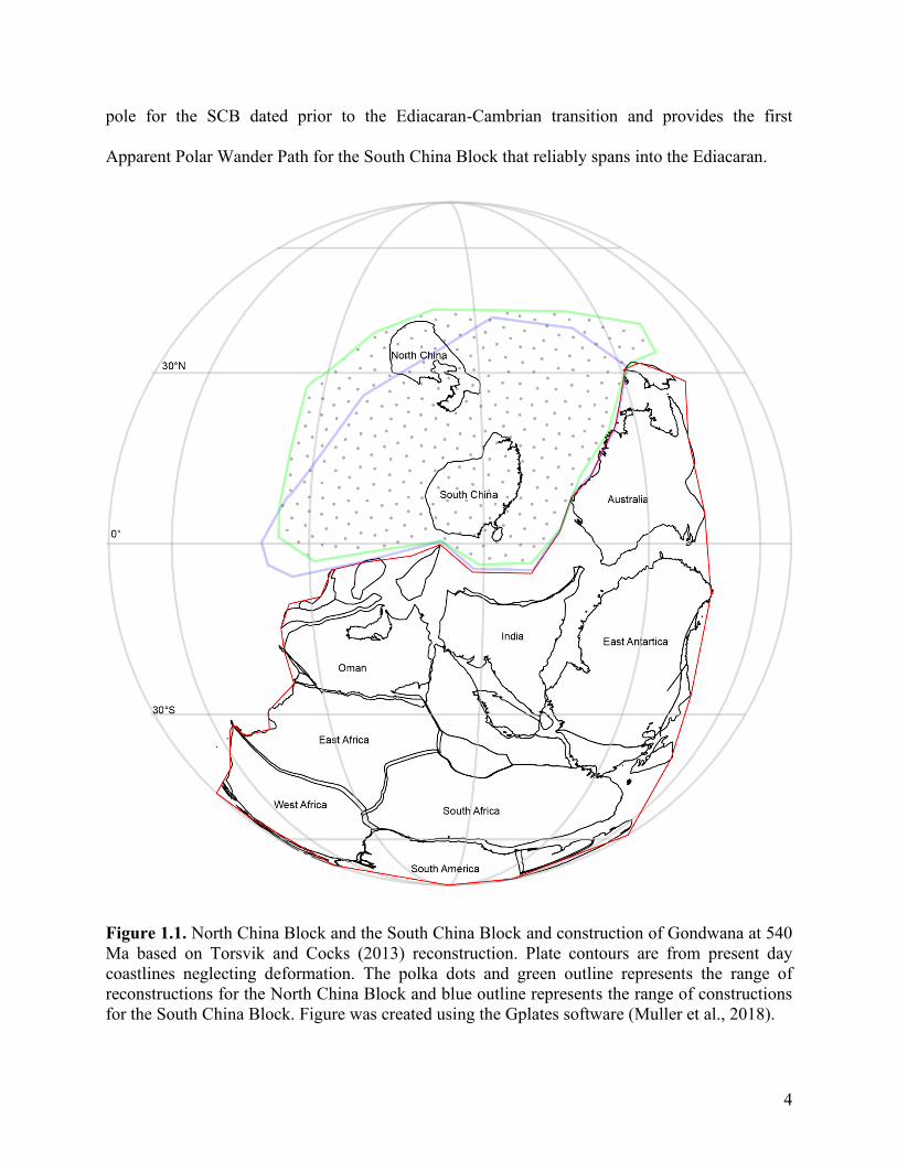
During the Ediacaran there was the final amalgamation of the supercontinent Gondwana which is
widely agreed upon as consisting of present-day Australia, India, Oman, South America, Africa,
and East Antarctica (Figure 1.1) (Veevers, 2004; Cawood et al., 2018; Li et al., 2018; Torsvik
and Cocks 2013). Major continents not accounted for as being part of Gondwana are Laurentia,
Baltica, and Siberia (Torsvik and Cocks, 2013). Often not included in reconstructions are the
North China Block (NCB) and the South China Block (SCB) due to the lack of reliable
paleomagnetic data. The SCB is of particular interest as it contains many well-preserved biota
and geochemical signatures, though due to lack of paleomagnetic data has been modelled in a
plethora of different locations in the global paleogeographic maps (Li et al., 2018). Chapter 3 of
this thesis reviews our study on rocks that span in age from the beginning of the Ediacaran to the
early Cambrian from the SCB. The results of this study provide the first reliable paleomagnetic
4
pole for the SCB dated prior to the Ediacaran-Cambrian transition and provides the first
Apparent Polar Wander Path for the South China Block that reliably spans into the Ediacaran.
Figure 1.1. North China Block and the South China Block and construction of Gondwana at 540
Ma based on Torsvik and Cocks (2013) reconstruction. Plate contours are from present day
coastlines neglecting deformation. The polka dots and green outline represents the range of
reconstructions for the North China Block and blue outline represents the range of constructions
for the South China Block. Figure was created using the Gplates software (Muller et al., 2018).

5
Chapter 2: Computation of magnetic anomalies caused by
two dimensional structures of arbitrary shape: derivation
and Matlab implementation1
2.1. Introduction
Talwani and Heirtzler (1964) were first to examine a non-magnetic space containing a uniformly
magnetized two-dimensional structure approximated by a polygonal prism and to suggest a
numerical and computational technique of the forward modeling. A magnetic anomaly above the
magnetized body was calculated by analytical formulae using summation of the anomalies due to
semi-infinite prisms limited on one side by a segment of the polygon. The derivation of the
mathematical expression for the magnetic anomaly over a two-dimensional body of polygonal
cross section was first done in Talwani and Heirtzler (1962). Certainly, it was not the first
approach to the problem, a comprehensive review of algorithms and approaches employed prior
to 1962 is given in Talwani and Heirtzler (1962). The algorithm was, however, derived
specifically for the computation using digital computers and therefore was the first algorithm of
such kind.
Since 1964, forward calculations of magnetic anomalies caused by two-dimensional (2-D) and
three-dimensional (3-D) bodies have progressed significantly. Talwani (1965) developed a new
1 A version of this paper has been published as:
Kravchinsky, V. A., Hnatyshin, D., Lysak, B., & Alemie, W. (2019). Computation of magnetic anomalies caused by two dimensional structures
of arbitrary shape: derivation and Matlab implementation. Geophysical Research Letters, https://doi.org/10.1029/2019GL082767.
6
algorithm to compute the three-dimensional magnetic anomaly for geological bodies of arbitrary
shape. Since, both 2- and 3-D forward problems have been developed in various alternative
ways. A comprehensive overview of the progress and approaches of the 2-D modeling since
1964 is provided in introductions from Kostrov (2007) and Jeshvaghani and Darijani (2014).
Our initial motivation was to create a Matlab program for educational purposes and for the rapid
interpretation of magnetic data. The algorithm of Talwani and Heirtzler (1964) would provide a
stable 2-D solution for variety of geological situations. This algorithm is a very effective for
magnetic surveys and the publication is the most cited among all existing magnetic forward
modeling methods. The first version of our software, however, produced some incorrect
anomalies in a number of theoretically modeled situations. Therefore, in this study, we
reappraise the derivation that leads us to a different from the Talwani and Heirtzler (1964)
solution. Both solutions are compared and discussed below. Further we develop a Matlab p-
coded and executable software that has user friendly GUI. The software is a freeware for
research and education purposes and can be redistributed among users. Any use of the software
should refer to this publication. The software can be downloaded from
www.ualberta.ca/vadim/software.htm.
2.2. Important Concepts
Here we introduce the important concepts and notation used for the derivation:

7
A) Magnetic Susceptibility (𝜒) - dimensionless. An object’s magnetic susceptibility is the
constant that indicates how much a material is magnetized in response to the local magnetic
field.
B) Magnetization (M) - Units = A/m. Magnetic fields can align the magnetic moments of
individual atoms within a material based on that material's magnetic susceptibility. The net
magnetic moment of the material per unit volume is magnetization.
C) Induced Magnetization (MI) is the magnetization associated with the proportion of the
material that is aligned with the Earth's magnetic field according to its current inclination and
declination.
D) Induced Inclination / Declination. Inclination is the angle the Earth's magnetic field makes
with respect with the horizontal. Positive angles are defined as angles that are directed below the
horizon. Declination is the difference in angle between true north and horizontal projection of
Earth's present day magnetic field. Values increase in the clockwise direction (0o for North, 90o
for East, etc.).
8
E) Remnant Magnetization (MR) is any preserved magnetization not associated with induced
magnetization. Often this is magnetization is associated with the formation of the rock/sediment,
or may be associated with recrystalization events (e.g. metamorphism), it is dependent on the
direction of the Earth’s magnetic field at the time of its acquisition.
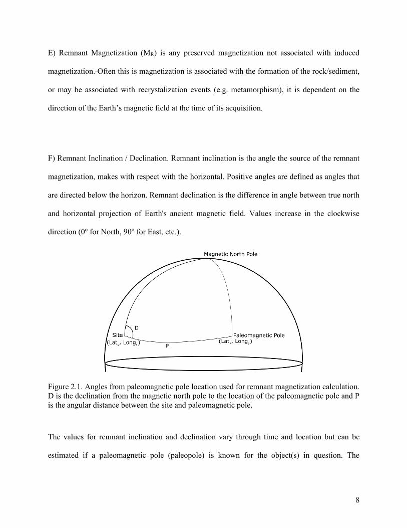
F) Remnant Inclination / Declination. Remnant inclination is the angle the source of the remnant
magnetization, makes with respect with the horizontal. Positive angles are defined as angles that
are directed below the horizon. Remnant declination is the difference in angle between true north
and horizontal projection of Earth's ancient magnetic field. Values increase in the clockwise
direction (0o for North, 90o for East, etc.).
Figure 2.1. Angles from paleomagnetic pole location used for remnant magnetization calculation.
D is the declination from the magnetic north pole to the location of the paleomagnetic pole and P
is the angular distance between the site and paleomagnetic pole.
The values for remnant inclination and declination vary through time and location but can be
estimated if a paleomagnetic pole (paleopole) is known for the object(s) in question. The
9
paleopole latitude and paleopole longitude can be converted into inclination (I) and declination
(D) using MagMod and is based on the following formulas:
𝑃 = sin−1[sin(𝑙𝑎𝑡𝑠) sin(𝑙𝑎𝑡𝑝) + cos(𝑙𝑎𝑡𝑝) cos|𝑙𝑜𝑛𝑔𝑠 − 𝑙𝑜𝑛𝑔𝑝|] (2.1)
𝐼 = tan−1[2 tan(𝑃)] (2.2)
𝐷 = sin−1 [sin|𝑙𝑜𝑛𝑔𝑠 − 𝑙𝑜𝑛𝑔𝑝| ∗cos(𝑙𝑎𝑡𝑝)
cos(𝑃)] (2.3)
where P = paleolatitude, lats is the latitude of the site, lons is the longitude of the site, latp is the
latitude of the paleopole and lonp is the longitude of the paleopole.
G) Total magnetization of the subsurface structure or small element is a superposition of the
induced and remnant magnetizations:
H) A magnetic anomaly is the magnetic field associated with unknown bodies within the
subsurface normalized against the local magnetic field (i.e. Earth's magnetic field).
2.3. Calculating Anomalies
Consider that there exists an elemental volume contained within an irregularly shaped body. This
elemental volume extends from negative to positive infinity in the y-direction. Bodies of
10
irregular shapes can be approximated by a polygon, which can be and reduced to solving semi-
infinite two-dimensional polygons (Talwani and Heirtzler, 1962). Now consider a small volume
element with dimensions dx, dy, dz (Figure 2.1A) located in the geomagnetic field. The total
magnetization of the volume is a superposition of both induced and remnant magnetizations
which co-exist.
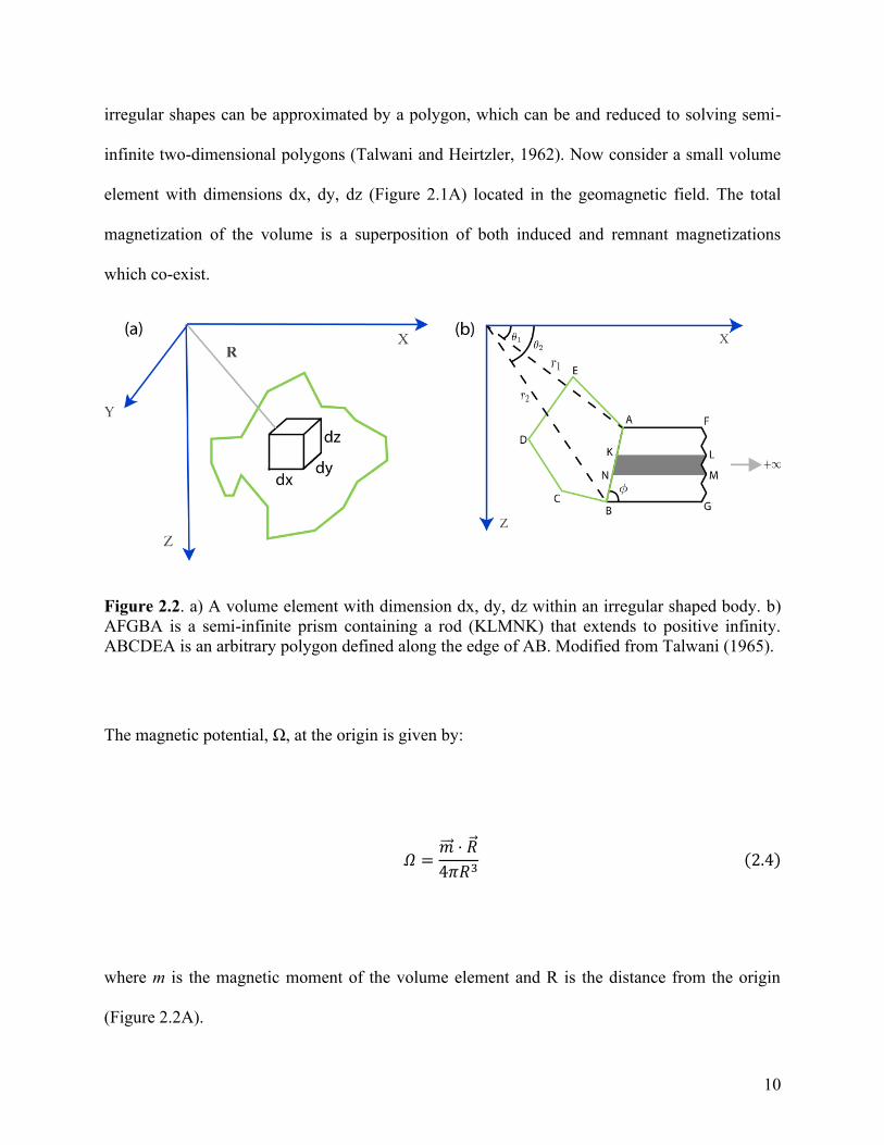
Figure 2.2. a) A volume element with dimension dx, dy, dz within an irregular shaped body. b)
AFGBA is a semi-infinite prism containing a rod (KLMNK) that extends to positive infinity.
ABCDEA is an arbitrary polygon defined along the edge of AB. Modified from Talwani (1965).
The magnetic potential, Ω, at the origin is given by:
𝛺 =�⃗⃗� ⋅ �⃗�
4𝜋𝑅3(2.4)
where m is the magnetic moment of the volume element and R is the distance from the origin
(Figure 2.2A).
11
Assuming that this volume element contains a uniform intensity of magnetization, 𝐽, the
magnetic moment of a body can be represented as:
�⃗⃗� = 𝐽 𝑑𝑥𝑑𝑦𝑑𝑧 (2.5)
The magnetic moment in terms of Cartesian coordinates x, y, z, can be written as:
𝛺 =𝐽𝑥𝑥 + 𝐽𝑦𝑦 + 𝐽𝑧𝑧
4𝜋(𝑥2 + 𝑦2 + 𝑧2)3
2⁄𝑑𝑥𝑑𝑦𝑑𝑧 (2.6)
Using the assumption that the body extends from negative infinity to positive infinity in the y-
direction and then integrating equation 2.6 with respect to y, the magnetic potential has the form:
𝛺 = ∫𝐽𝑥𝑥 + 𝐽𝑦𝑦 + 𝐽𝑧𝑧
4𝜋(𝑥2 + 𝑦2 + 𝑧2)3
2⁄𝑑𝑦
∞
−∞
=(𝐽𝑥𝑥 + 𝐽𝑧𝑧)
2𝜋(𝑥2 + 𝑧2)𝑑𝑥𝑑𝑧 (2.7)

12
The vertical (V) and horizontal (H) components of the magnetic strength can be derived by
differentiating equation (2.7) with respect to z and x respectively and results in the following
equations results in the following equations:
𝑉 = −𝜕𝛺
𝜕𝑧=
2𝐽𝑥𝑥𝑧 − 𝐽𝑧(𝑥2 − 𝑧2)
2𝜋(𝑥2 + 𝑧2)2𝑑𝑥𝑑𝑧 (2.8)
𝐻 = −𝜕𝛺
𝜕𝑥=
2𝐽𝑧𝑥𝑧 + 𝐽𝑥(𝑥2 − 𝑧2)
2𝜋(𝑥2 + 𝑧2)2𝑑𝑥𝑑𝑧 (2.9)
Assuming that the body extents to positive infinity in the x-direction we can simplify equations
(2.8) and (2.9) by integrating from x to positive infinity, which results in:
𝑉 = ∫2𝐽𝑥𝑥𝑧 − 𝐽𝑧(𝑥
2 − 𝑧2)
2𝜋(𝑥2 + 𝑧2)2𝑑𝑥𝑑𝑧
∞
𝑥
=𝐽𝑥𝑧 − 𝐽𝑧𝑥
2𝜋(𝑥2 + 𝑧2)𝑑𝑧 (2.10)
𝐻 = ∫2𝐽𝑧𝑥𝑧 + 𝐽𝑥(𝑥
2 − 𝑧2)
2𝜋(𝑥2 + 𝑧2)2𝑑𝑥𝑑𝑧 =
∞
𝑥
𝐽𝑥𝑥 − 𝐽𝑧𝑧
2𝜋(𝑥2 + 𝑧2)𝑑𝑧 (2.11)
Equations (2.10) and (2.11) are the components produced by the rod KLMNK in Figure 2.2b.
The resulting integrating these equations from z1 to z2, the magnetic field strength for the prism
AFGBA in Figure 2.2b produces equations that can be expressed in the simplified form as shown
below (see detailed step by step derivation in the Supporting Information file):
13
𝑉 =1
2𝜋(𝐽𝑥𝑄 − 𝐽𝑧𝑃) (2.12)
𝐻 =1
2𝜋(𝐽𝑧𝑄 + 𝐽𝑥𝑃) (2.13)
where,
𝑄 = 𝛾𝑧2 𝑙𝑛 (
𝑟2𝑟1
) − 𝛿𝛾𝑧𝛾𝑥(𝛼2 − 𝛼1) (2.14)
𝑃 = 𝛾𝑧𝛾𝑥 𝑙𝑛 (𝑟2𝑟1
) + 𝛿𝛾𝑧2(𝛼2 − 𝛼1) (2.15)
𝛾𝑧 = 𝑧21
√𝑥212 + 𝑧21
2(2.16)
𝛾𝑥 = 𝑥21
√𝑥212 + 𝑧21
2(2.17)
𝑟1 = √𝑥12 + 𝑧1
2 (2.18)
𝑟2 = √𝑥22 + 𝑧2
2 (2.19)
𝛼1 = 𝑡𝑎𝑛−1 (𝛿(𝑧1 + 𝑔𝑥1)
𝑥1 − 𝑔𝑧1) (2.20)
𝛼2 = 𝑡𝑎𝑛−1 (𝛿(𝑧2 + 𝑔𝑥2)
𝑥2 − 𝑔𝑧2) (2.21)
𝑔 = 𝑥2 − 𝑥1
𝑧2 − 𝑧1=
𝑥21
𝑧21
(2.22)

14
𝛿 = 1 if 𝑥1 > 𝑔𝑧1, 𝛿 = −1 if 𝑥1 < 𝑔𝑧1
For an arbitrarily shaped polygon a point xi, zi represents a corner of the polygon and a point xi+1,
zi+1 to be the next corner of the polygon. Equations (2.12) and (2.13) represent the magnetic
strength of the rectangular region AFGBA for only one side of the polygon. For a polygon with
n-sides there is a n number of prisms of the same form as AFGBA. Calculation for a positive
anomaly requires calculation of the polygon clockwise with reference to the origin as depicted in
Figure 2.4 and summing the contribution of each side.
To evaluate the total intensity anomaly, T, we need to sum the projection of H and V along the
direction of the total field. This can be done by manipulating the magnetization vectors
associated with total magnetization (J) while using the convention shown in Figure 2.3. In
general, total magnetization is a superposition of induced (Ji) and remnant magnetization (Jr)
which are given by:
15
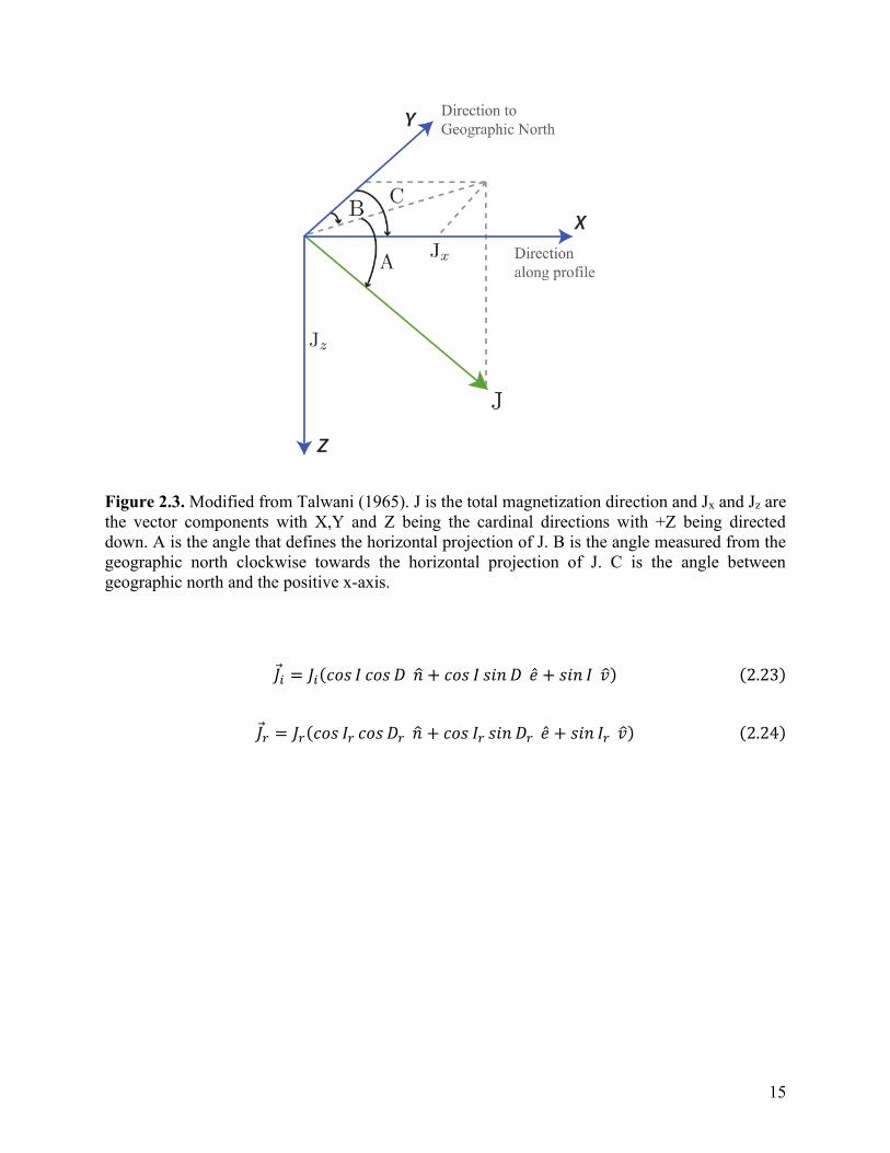
Figure 2.3. Modified from Talwani (1965). J is the total magnetization direction and Jx and Jz are
the vector components with X,Y and Z being the cardinal directions with +Z being directed
down. A is the angle that defines the horizontal projection of J. B is the angle measured from the
geographic north clockwise towards the horizontal projection of J. C is the angle between
geographic north and the positive x-axis.
𝐽 𝑖 = 𝐽𝑖(𝑐𝑜𝑠 𝐼 𝑐𝑜𝑠 𝐷 �̂� + 𝑐𝑜𝑠 𝐼 𝑠𝑖𝑛 𝐷 �̂� + 𝑠𝑖𝑛 𝐼 𝑣) (2.23)
𝐽 𝑟 = 𝐽𝑟(𝑐𝑜𝑠 𝐼𝑟 𝑐𝑜𝑠 𝐷𝑟 �̂� + 𝑐𝑜𝑠 𝐼𝑟 𝑠𝑖𝑛 𝐷𝑟 �̂� + 𝑠𝑖𝑛 𝐼𝑟 𝑣) (2.24)
16
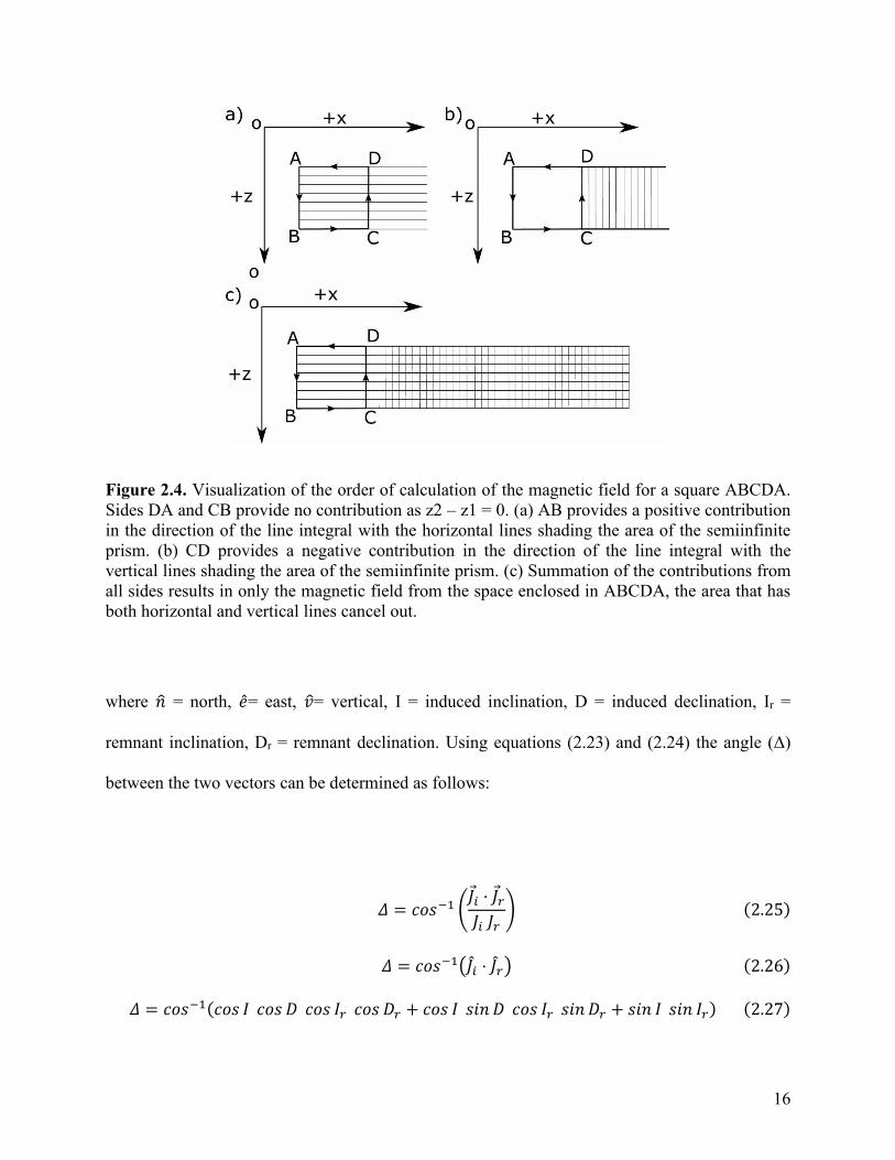
Figure 2.4. Visualization of the order of calculation of the magnetic field for a square ABCDA.
Sides DA and CB provide no contribution as z2 – z1 = 0. (a) AB provides a positive contribution
in the direction of the line integral with the horizontal lines shading the area of the semiinfinite
prism. (b) CD provides a negative contribution in the direction of the line integral with the
vertical lines shading the area of the semiinfinite prism. (c) Summation of the contributions from
all sides results in only the magnetic field from the space enclosed in ABCDA, the area that has
both horizontal and vertical lines cancel out.
where �̂� = north, �̂�= east, 𝑣= vertical, I = induced inclination, D = induced declination, Ir =
remnant inclination, Dr = remnant declination. Using equations (2.23) and (2.24) the angle (Δ)
between the two vectors can be determined as follows:
𝛥 = 𝑐𝑜𝑠−1 (𝐽 𝑖 ⋅ 𝐽 𝑟𝐽𝑖 𝐽𝑟
) (2.25)
𝛥 = 𝑐𝑜𝑠−1(𝐽𝑖 ⋅ 𝐽𝑟) (2.26)
𝛥 = 𝑐𝑜𝑠−1(𝑐𝑜𝑠 𝐼 𝑐𝑜𝑠 𝐷 𝑐𝑜𝑠 𝐼𝑟 𝑐𝑜𝑠 𝐷𝑟 + 𝑐𝑜𝑠 𝐼 𝑠𝑖𝑛 𝐷 𝑐𝑜𝑠 𝐼𝑟 𝑠𝑖𝑛 𝐷𝑟 + 𝑠𝑖𝑛 𝐼 𝑠𝑖𝑛 𝐼𝑟) (2.27)
17
This angle Δ can be used to calculate the magnitude of the total magnetization (J) as well as its
inclination (A) and declination (B). Using the cosine law the total magnetization J is defined as:
𝐽2 = 𝐽𝑖2 + 𝐽𝑟
2 − 2𝐽𝑖 𝐽𝑟 𝑐𝑜𝑠 𝛥 (2.28)
To determine the inclination (A) and declination (B) of J we split Ji and Jr into their horizontal
(JiH and JrH, respectively) and vertical components (JiV and JrV, respectively). Inclination is then
derived as follows:
𝐽𝑉 = 𝐽𝑖𝑉 + 𝐽𝑟𝑉 (2.29)
𝐽𝑉 = 𝐽𝑖 𝑠𝑖𝑛 𝐼 + 𝐽𝑟 𝑠𝑖𝑛 𝐼𝑟 (2.30)
𝐽 𝑠𝑖𝑛 𝐴 = 𝐽𝑖 𝑠𝑖𝑛 𝐼 + 𝐽𝑟 𝑠𝑖𝑛 𝐼𝑟 (2.31)
𝑠𝑖𝑛 𝐴 =𝐽𝑖 𝑠𝑖𝑛 𝐼 + 𝐽𝑟 𝑠𝑖𝑛 𝐼𝑟
𝐽(2.32)
𝐴 = 𝑠𝑖𝑛−1 (𝐽𝑖 𝑠𝑖𝑛 𝐼 + 𝐽𝑟 𝑠𝑖𝑛 𝐼𝑟
𝐽) (2.33)
Similarly, declination it derived as follows:
𝐽𝐻 = 𝐽 𝑐𝑜𝑠 𝐴 (2.34)
𝐽𝐻 = 𝐽𝑖𝐻 + 𝐽𝑟𝐻 (2.35)
18
𝐽𝐻 = 𝐽𝑖 𝑐𝑜𝑠 𝐼 + 𝐽𝑟 𝑐𝑜𝑠 𝐼𝑟 (2.36)
𝐽𝐻�̂� = 𝐽𝐻 𝑐𝑜𝑠 𝐵 (2.37)
𝐽𝐻 𝑐𝑜𝑠 𝐵 = 𝐽𝑖𝐻�̂� + 𝐽𝑟𝐻�̂� (2.38)
𝐽𝐻 𝑐𝑜𝑠 𝐵 = 𝐽𝑖𝐻 𝑐𝑜𝑠 𝐷 + 𝐽𝑟𝐻 𝑐𝑜𝑠 𝐷𝑟 (2.39)
𝐽𝐻 𝑐𝑜𝑠 𝐵 = 𝐽𝑖 𝑐𝑜𝑠 𝐼 𝑐𝑜𝑠 𝐷 + 𝐽𝑟 𝑐𝑜𝑠 𝐼𝑟 𝑐𝑜𝑠 𝐷𝑟 (2.40)
𝑐𝑜𝑠 𝐵 =𝐽𝑖 𝑐𝑜𝑠 𝐼 𝑐𝑜𝑠 𝐷 + 𝐽𝑟 𝑐𝑜𝑠 𝐼𝑟 𝑐𝑜𝑠 𝐷𝑟
𝐽𝐻(2.41)
𝐵 = 𝑐𝑜𝑠−1 (𝐽𝑖 𝑐𝑜𝑠 𝐼 𝑐𝑜𝑠 𝐷 + 𝐽𝑟 𝑐𝑜𝑠 𝐼𝑟 𝑐𝑜𝑠 𝐷𝑟
𝐽 𝑐𝑜𝑠 𝐴) (2.42)
The intensity of magnetization of magnetization in the x and z directions in the terms of total
magnetization, J, in terms of A, B, C can be defined as:
𝐽𝑥 = 𝐽 cos(𝐴) cos(𝐶 − 𝐵) (2.43)
𝐽𝑧 = 𝐽 sin(𝐴) (2.44)
The total intensity anomaly (T) can then be defined as:
𝑇 = 𝑉 sin(𝐴) + 𝐻 cos(𝐴) cos(𝐶 − 𝐵) (2.45)
19
2.4. Discussion
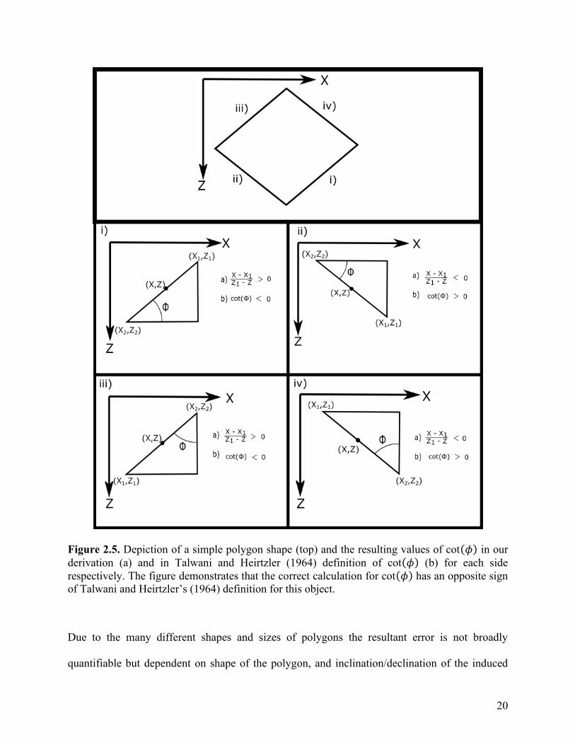
Upon a rederivation of the original Talwani and Heirtzler (1964) algorithm we found three
explicit differences and errors in Talwani and Heirtzler’s (1964) derivation. The first error began
in the definition of 𝑥. Figure 2.5 demonstrates the resultant difference between the two
expressions for a polygon. Continuing derivation of the magnetic fields using Talwani and
Heirtzler (1964) definition for 𝑥, it was evident that the definition for θ1 and θ2 are not equivalent
to the angle the corners of the side make with the origin as depicted in Figure 2.2a. The final
issue found in derivation was the definition of a 𝛿 term. In Talwani and Heirtzlers (1964) this
term was assumed to value 1, indicating that they did not account for the impact of the absolute
value in the derivation.
20
Figure 2.5. Depiction of a simple polygon shape (top) and the resulting values of cot(𝜙) in our
derivation (a) and in Talwani and Heirtzler (1964) definition of cot(𝜙) (b) for each side
respectively. The figure demonstrates that the correct calculation for cot(𝜙) has an opposite sign
of Talwani and Heirtzler’s (1964) definition for this object.
Due to the many different shapes and sizes of polygons the resultant error is not broadly
quantifiable but dependent on shape of the polygon, and inclination/declination of the induced
21
magnetic field. To demonstrate the potential differences produced by different derivations, we
have calculated the induced magnetic field produced from a diamond with three different
inclinations and compare also with the method of Won and Bevis (1987). The method of Won
and Bevis (1987) who derived the magnetic anomaly due to a polygonal cylinder in a similar
matter to ours but using references to vertex coordinates to reduce references to angular
quantities and trigonometric identities. Figure 2.6 illustrates the comparison of the magnetic
anomalies computed using the six different algorithms: (i) Talwani and Heirtzler (1964), (ii) our
rederivation using Talwani and Heirtzlers (1964) definition of
𝑥 and accounting for corrected 𝛿, (iii) definition of 𝑥 and corrected θ, (iv) definition of 𝑥 and
accounting for the corrected 𝛿 and θ term, (v) robust derivation from first principles, and (vi)
Won and Bevis (1987). We find that the results for (i), (v) and (iv) are very similar. The errors
inherent in the original derivation of Talwani and Heirtzler (1964), particularly the definitions of
θ1, θ2 and δ, by removal compensate for each other to produce results that approximately agree
with the properly derived solution provided by our derivation. However, when the corrections for
θ1, θ2 and δ are applied independently they produce the same incorrect anomaly, which indicates
that these errors had to be made dependently otherwise it would produce incorrect anomalies.
We recommend the solution produced by Talwani and Heirtzler (1964) be avoided, as it cannot
be guaranteed to work for all possible shapes and cases. It is, however, clear that the errors were
fundamental and that when corrected the original algorithm of Talwani and Heirtzler (1964)
produced significant differences in the modeled magnetic field (see Supporting Information file).
22
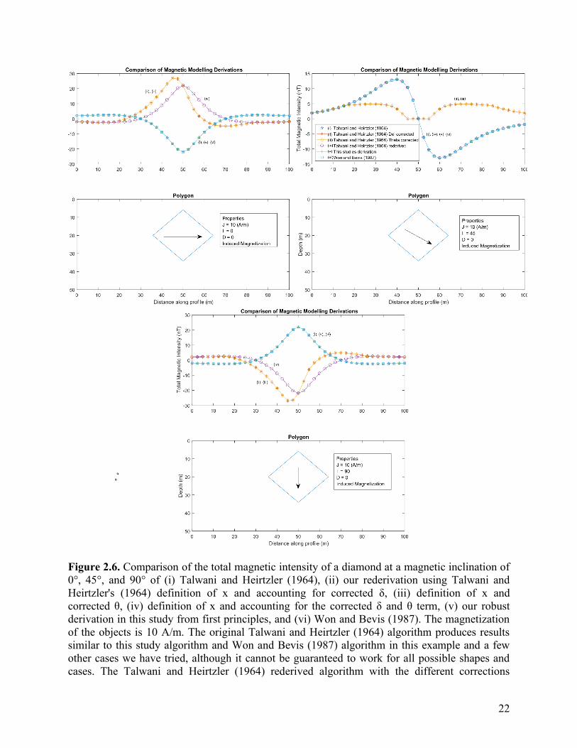
Figure 2.6. Comparison of the total magnetic intensity of a diamond at a magnetic inclination of
0°, 45°, and 90° of (i) Talwani and Heirtzler (1964), (ii) our rederivation using Talwani and
Heirtzler's (1964) definition of x and accounting for corrected δ, (iii) definition of x and
corrected θ, (iv) definition of x and accounting for the corrected δ and θ term, (v) our robust
derivation in this study from first principles, and (vi) Won and Bevis (1987). The magnetization
of the objects is 10 A/m. The original Talwani and Heirtzler (1964) algorithm produces results
similar to this study algorithm and Won and Bevis (1987) algorithm in this example and a few
other cases we have tried, although it cannot be guaranteed to work for all possible shapes and
cases. The Talwani and Heirtzler (1964) rederived algorithm with the different corrections
23
applied together and independently produces offset results when calculated to a diamond for
different inclinations.
2.5. Conclusions
The resulting expressions for the components of the magnetic field (2.12, 2.13) are not equal to
the expressions derived by Talwani and Heirtzler (1964). The discrepancy between our
derivation and Talwani and Heirtzler (1964) lies in the definition of the variable x, definition of
the angles θ1 and θ2, and the dismissal of an absolute value. Talwani and Heirtzler (1964) have
erroneous definitions. Detailed rederivation of Talwani and Heirtzler formulas to calculate
magnetic anomalies caused by two dimensional structures of arbitrary shape is given in the
appendix. The rederived final solution is different from the original published formulas of
Talwani and Heirtzler (1964) and produces incorrect anomalies (Figure 2.5), therefore we
strongly recommend to use our algorithm derived in this study to avoid any fundamental errors
in calculating the anomalies.
Software and data availability
The free software and example data are available for download from
www.ualberta.ca/~vadim/software.htm. This publication has to be referred with any use of the
software.
24
Acknowledgment
We are thankful K. Bianchi for his help with derivation confirmation, S. Alhashwa for his help at
the initial stage of the project and F. Caratori Tontini for his in-depth verification of our
derivations and discussion that led to essential improvement of this manuscript. The project was
funded by the Natural Sciences and Engineering Research Council of Canada of V.A.K.
(NSERC grant RGPIN-2019-04780). This study forms part of B.L. M.Sc. thesis at the University
of Alberta.
References
Jeshvaghani, M. S., & Darijani, M. (2014). Two-dimensional geomagnetic forward modeling
using adaptive finite element method and investigation of the topographic effect. Journal of
Applied Geophysics, 105, 169-179.
Kostrov, N. P. (2007). Calculation of magnetic anomalies caused by 2D bodies of arbitrary shape
with consideration of demagnetization. Geophysical prospecting, 55(1), 91-115.
Lelievre, P.G., & Oldenburg, D.W. (2006). Magnetic forward modelling and inversion for high
susceptibility. Geophysical Journal International, 166 (1), 76-90.
Talwani, M., & Heirtzler, J. R., 1962. The Mathematical Expression for the Magnetic Anomaly
over a Two-Dimensional Body of Polygonal Cross Section. Lamont Doherty Geol. Obs.
Columbia Univ., Tech. Rep. 6.
Talwani, M., & Heirtzler, J. R., 1964. Computation of magnetic anomalies caused by two
dimensional structures of arbitrary shape. Computers in the mineral industries, part 1: Stanford
University publications, Geol. Sciences, 9, 464-480.

25
Talwani, M. (1965). Computation with the help of a digital computer of magnetic anomalies
caused by bodies of arbitrary shape. Geophysics, 30(5), 797-817.
Won, I. J., & Bevis, M. (1987). Computing the gravitational and magnetic anomalies due to a
polygon: Algorithms and Fortran subroutines. Geophysics, 52(2), 232-238.
26
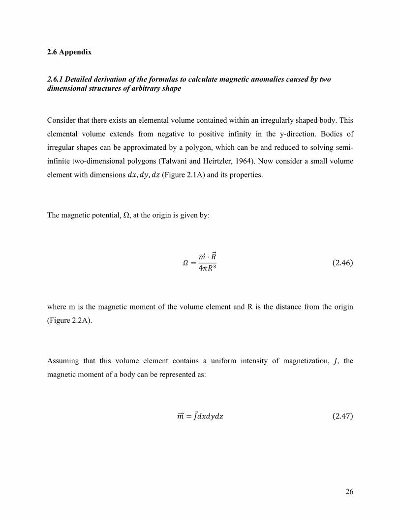
2.6 Appendix
2.6.1 Detailed derivation of the formulas to calculate magnetic anomalies caused by two
dimensional structures of arbitrary shape
Consider that there exists an elemental volume contained within an irregularly shaped body. This
elemental volume extends from negative to positive infinity in the y-direction. Bodies of
irregular shapes can be approximated by a polygon, which can be and reduced to solving semi-
infinite two-dimensional polygons (Talwani and Heirtzler, 1964). Now consider a small volume
element with dimensions 𝑑𝑥, 𝑑𝑦, 𝑑𝑧 (Figure 2.1A) and its properties.
The magnetic potential, Ω, at the origin is given by:
𝛺 =�⃗⃗� ⋅ �⃗�
4𝜋𝑅3(2.46)
where m is the magnetic moment of the volume element and R is the distance from the origin
(Figure 2.2A).
Assuming that this volume element contains a uniform intensity of magnetization, 𝐽, the
magnetic moment of a body can be represented as:
�⃗⃗� = 𝐽 𝑑𝑥𝑑𝑦𝑑𝑧 (2.47)

27
The magnetic moment in terms of Cartesian coordinates 𝑥, 𝑦, 𝑧, can then be written as:
𝛺 =𝐽𝑥𝑥 + 𝐽𝑦𝑦 + 𝐽𝑧𝑧
4𝜋(𝑥2 + 𝑦2 + 𝑧2)3
2⁄𝑑𝑥𝑑𝑦𝑑𝑧 (2.48)
Using the assumption that the body extends from negative infinity to positive infinity in the y-
direction and then integrating equation 3 with respect to y, the magnetic potential has the form
𝛺 = ∫𝐽𝑥𝑥 + 𝐽𝑦𝑦 + 𝐽𝑧𝑧
4𝜋(𝑥2 + 𝑦2 + 𝑧2)3
2⁄𝑑𝑦
∞
−∞
=(𝐽𝑥𝑥 + 𝐽𝑧𝑧)
2𝜋(𝑥2 + 𝑧2)𝑑𝑥𝑑𝑧 (2.49)
The vertical (V) and horizontal (H) components of the magnetic strength can be derived by
differentiating equation (2.49) with respect to z and x respectively, and results in the following
equations:
𝑉 = −𝜕𝛺
𝜕𝑧=
2𝐽𝑥𝑥𝑧 − 𝐽𝑧(𝑥2 − 𝑧2)
2𝜋(𝑥2 + 𝑧2)2𝑑𝑥𝑑𝑧 (2.50)
𝐻 = −𝜕𝛺
𝜕𝑥=
2𝐽𝑧𝑥𝑧 + 𝐽𝑥(𝑥2 − 𝑧2)
2𝜋(𝑥2 + 𝑧2)2𝑑𝑥𝑑𝑧 (2.51)
Assuming that the body extents to positive infinity in the x-direction we can simplify equations
(5) and (6) by integrating from x to positive infinity, which results in:
28
𝑉 = ∫2𝐽𝑥𝑥𝑧 − 𝐽𝑧(𝑥
2 − 𝑧2)
2𝜋(𝑥2 + 𝑧2)2𝑑𝑥𝑑𝑧
∞
𝑥
=𝐽𝑥𝑧 − 𝐽𝑧𝑥
2𝜋(𝑥2 + 𝑧2)𝑑𝑧 (2.52)
𝐻 = ∫2𝐽𝑧𝑥𝑧 + 𝐽𝑥(𝑥
2 − 𝑧2)
2𝜋(𝑥2 + 𝑧2)2𝑑𝑥𝑑𝑧 =
∞
𝑥
𝐽𝑥𝑥 − 𝐽𝑧𝑧
2𝜋(𝑥2 + 𝑧2)𝑑𝑧 (2.53)
Equations (2.52) and (2.53) are the components produced by the rod KLMNK in Figure 2.1B.
Integrating these equations from z1 to z2, the magnetic field strength for the prism AFGBA in
Fig. 1B can be calculated.
𝑉 = ∫𝐽𝑥𝑧 − 𝐽𝑧𝑥
2𝜋(𝑥2 + 𝑧2)𝑑𝑧
𝑧2
𝑧1
(2.54)
In order to compute this integral, consider taking a point on the side of a polygon (ABCDEA)
that makes up the region of interest (AFGBA). This enables us to find 𝑥 as a function of the
coordinates of the corners and 𝑧.
Let
𝑔 =𝑧2−𝑧1
𝑥2−𝑥1=
𝑥−𝑥1
𝑧−𝑧1(2.55)
Equation (2.55) can then be rearranged into,
𝑥 = 𝑔(𝑧 − 𝑧1) + 𝑥1 (2.56)

29
and then inserted into equation (2.54), which results in the following sets of equations,
𝑉 =1
2𝜋∫
𝐽𝑥𝑧 − 𝐽𝑧(𝑔(𝑧 − 𝑧1) + 𝑥1)
[𝑔(𝑧 − 𝑧1) + 𝑥1]2 + 𝑧2𝑑𝑧
𝑧2
𝑧1
(2.57)
𝑉 =1
2𝜋∫
(𝐽𝑥𝑧 − 𝑔𝐽𝑧)𝑧 − 𝐽𝑧(𝑥1 − 𝑔𝑧1)
(1 + 𝑔2)𝑧2 + 2𝑔(𝑥1 − 𝑔𝑧1)𝑧 + (𝑥1 − 𝑔𝑧1)2𝑑𝑧
𝑧2
𝑧1
(2.58)
We can rewrite this in simpler terms by letting
𝑎 = 1 + 𝑔2 (2.59)
𝑏 = 2𝑔(𝑥1 − 𝑔𝑧1)𝑧 (2.60)
𝑐 = (𝑥1 − 𝑔𝑧1)2 (2.61)
which results in,
𝑉 =1
2𝜋∫
(𝐽𝑥 − 𝑔𝐽𝑧)𝑧 − 𝐽𝑧(𝑥1 − 𝑔𝑧1)
𝑎𝑧2 + 𝑏𝑧 + 𝑐𝑑𝑧
𝑧2
𝑧1
(2.62)
These equations can be rewritten in terms of to 2 components,
𝑉 =1
2𝜋∫
(𝐽𝑥 − 𝑔𝐽𝑧)𝑧
𝑎𝑧2 + 𝑏𝑧 + 𝑐𝑑𝑧 −
1
2𝜋
𝑧2
𝑧1
∫𝐽𝑧(𝑥1 − 𝑔𝑧1)
𝑎𝑧2 + 𝑏𝑧 + 𝑐𝑑𝑧
𝑧2
𝑧1
(2.63)
30
𝑉 =(𝐽𝑥 − 𝑔𝐽𝑧)
2𝜋∫
𝑧
𝑎𝑧2 + 𝑏𝑧 + 𝑐𝑑𝑧 −
𝑧2
𝑧1
𝐽𝑧(𝑥1 − 𝑔𝑧1)
2𝜋∫
𝑑𝑧
𝑎𝑧2 + 𝑏𝑧 + 𝑐
𝑧2
𝑧1
(2.64)
𝑉 = 𝐼1 + 𝐼2 (2.65)
where,
𝐼1 =(𝐽𝑥 − 𝑔𝐽𝑧)
2𝜋∫
𝑧
𝑎𝑧2 + 𝑏𝑧 + 𝑐𝑑𝑧
𝑧2
𝑧1
(2.66)
𝐼2 = −𝐽𝑧(𝑥1 − 𝑔𝑧1)
2𝜋∫
𝑑𝑧
𝑎𝑧2 + 𝑏𝑧 + 𝑐
𝑧2
𝑧1
(2.67)
Equation (2.65) can be integrated using the following integral identities:
For:
𝐴 ≠ 0 (2.68)
4𝐴𝐶 − 𝐵2 > 0 (2.69)
∫𝑥𝑑𝑥
𝐴𝑥2 + 𝐵𝑥 + 𝐶=
1
2𝐴𝑙𝑛|𝐴𝑥2 + 𝐵𝑥 + 𝐶| −
𝐵
𝐴√4𝐴𝐶 − 𝐵2𝑡𝑎𝑛−1 (
2𝐴𝑥 + 𝐵
√4𝐴𝐶 − 𝐵2)
∫𝑑𝑥
𝐴𝑥2 + 𝐵𝑥 + 𝐶=
2
√4𝐴𝐶 − 𝐵2𝑡𝑎𝑛−1 (
2𝐴𝑥 + 𝐵
√4𝐴𝐶 − 𝐵2) (2.70)
To use these identities, we first check that the criteria are met for equation (2.68). First by
checking that 𝐴 ≠ 0. For the first criteria, equation (12) defines = 1 + 𝑔2 , which requires that
𝐴 > 0, which implies 𝐴 ≠ 0.
31
Checking 4𝐴𝐶 − 𝐵2 > 0 is done as follows:
𝐵 = 2𝑔(𝑥1 − 𝑔𝑧1) (2.71)
𝐶 = 𝑥1 − 𝑔𝑧1 (2.72)
4𝐴𝐶 − 𝐵2 = 4(1 + 𝑔2)(𝑥1 − 𝑔𝑧1)2 − (2𝑔(𝑥1 − 𝑔𝑧1))
2(2.73)
4𝐴𝐶 − 𝐵2 = 4(1 + 𝑔2)(𝑥1 − 𝑔𝑧1)2 − 4𝑔2(𝑥1 − 𝑔𝑧1))
2
4𝐴𝐶 − 𝐵2 = (𝑥1 − 𝑔𝑧1)2(4(1 + 𝑔2) − 4𝑔2)
4𝐴𝐶 − 𝐵2 = (𝑥1 − 𝑔𝑧1)2(4(1 + 𝑔2) − 4𝑔2)
4𝐴𝐶 − 𝐵2 = (𝑥1 − 𝑔𝑧1)2(4(1 + 𝑔2 − 𝑔2)
4𝐴𝐶 − 𝐵2 = 4(𝑥1 − 𝑔𝑧1)2 (2.74)
Since both criteria are met, we use the above identities to solve for I1 and I2.
𝐼1 =𝐽𝑥 − 𝑔𝐽𝑧
2𝜋[ 1
2𝑎(𝑙𝑛|𝑎𝑧2
2 + 𝑏𝑧2 + 𝑐| − 𝑙𝑛|𝑎𝑧12 + 𝑏𝑧1 + 𝑐|)
−𝑏
𝑎√4𝑎𝑐 − 𝑏2(𝑡𝑎𝑛−1 (
2𝑎𝑧2 + 𝑏
√4𝑎𝑐 − 𝑏2) − 𝑡𝑎𝑛−1 (
2𝑎𝑧1 + 𝑏
√4𝑎𝑐 − 𝑏2))
]
(2.75)
where,
𝑎𝑧22 + 𝑏𝑧2 + 𝑐 = (1 + 𝑔2)𝑧2
2 + 2𝑔(𝑥1 − 𝑔𝑧1)𝑧2 + (𝑥1 − 𝑔𝑧1)2
𝑎𝑧22 + 𝑏𝑧2 + 𝑐 = 𝑧2
2 + 𝑔2𝑧22 + 2𝑔𝑥1𝑧2 − 2𝑔2𝑧1𝑧2 + 𝑥1
2 + 𝑔2𝑧12 − 2𝑔𝑥1𝑧1
𝑎𝑧22 + 𝑏𝑧2 + 𝑐 = 𝑧2
2 + 𝑔2(𝑧22 − 2𝑧1𝑧2 + 𝑧1
2) + 2𝑔𝑥1𝑧2 − 2𝑔𝑥1𝑧1 + 𝑥12
𝑎𝑧22 + 𝑏𝑧2 + 𝑐 = 𝑧2
2 + 𝑔2(𝑧2 − 𝑧1)2 + 2𝑔𝑥1𝑧2 − 2𝑔𝑥1𝑧1 + 𝑥1
2
𝑎𝑧22 + 𝑏𝑧2 + 𝑐 = 𝑧2
2 + 𝑔2(𝑧2 − 𝑧1)2 + 2𝑔𝑥1(𝑧2 − 𝑧1) + 𝑥1
2

32
but, 𝑔(𝑧2 − 𝑧1) = 𝑥2 − 𝑥1, which then gives,
𝑎𝑧22 + 𝑏𝑧2 + 𝑐 = 𝑧2
2 + (𝑥2 − 𝑥1)2 + 2𝑥1(𝑥2 − 𝑥1) + 𝑥1
2 = 𝑧22 + 𝑥2
2 (2.76)
Similarly,
𝑎𝑧12 + 𝑏𝑧1 + 𝑐 = 𝑧1
2 + 𝑥12 (2.77)
By inspection of Figure 2.1B, the following relationship exists:
𝑟12 = 𝑧1
2 + 𝑥12 = 𝑎𝑧1
2 + 𝑏𝑧1 + 𝑐 (2.78)
𝑟22 = 𝑧2
2 + 𝑥22 = 𝑎𝑧2
2 + 𝑏𝑧2 + 𝑐 (2.79)
By inspection equation 2.79 is equivalent to its absolute value:
𝑟12 = |𝑎𝑧1
2 + 𝑏𝑧1 + 𝑐| = |𝑟12| (2.80)
𝑟22 = |𝑎𝑧2
2 + 𝑏𝑧2 + 𝑐| = |𝑟22| (2.81)
therefore,

33
𝑙𝑛|𝑎𝑧12 + 𝑏𝑧1 + 𝑐| = 𝑙𝑛|𝑟1
2| = 𝑙𝑛 𝑟12 (2.82)
𝑙𝑛|𝑎𝑧22 + 𝑏𝑧2 + 𝑐| = 𝑙𝑛|𝑟2
2| = 𝑙𝑛 𝑟22 (2.83)
The terms 2𝑎𝑧1,2 + 𝑏 in equation (2.75) can be rewritten as follows:
2𝑎𝑧2 + 𝑏 = 2(𝑔2 + 1)𝑧2 + 2𝑔(𝑥1 − 𝑔𝑧1)
2𝑎𝑧2 + 𝑏 = 2𝑔2𝑧2 + 2𝑧2 + 2𝑔𝑥1 − 2𝑔2𝑧1
2𝑎𝑧2 + 𝑏 = 2𝑔2(𝑧2 − 𝑧1) + 2𝑧2 + 2𝑔𝑥1
recall 𝑔(𝑧2 − 𝑧1) = 𝑥2 − 𝑥1, so that,
2𝑎𝑧2 + 𝑏 = 2𝑔(𝑥2 − 𝑥1) + 2𝑧2 + 2𝑔𝑥1 = 2(𝑧2 + 𝑔𝑥2) (2.84)
similarly,
2𝑎𝑧1 + 𝑏 = 2(𝑧1 + 𝑔𝑥1) (2.85)
(17)
The term √4𝑎𝑐 − 𝑏2is rewritten as follows:
√4𝑎𝑐 − 𝑏2 = √4(1 + 𝑔2)(𝑥1 − 𝑔𝑧1)2 − (2𝑔(𝑥1 − 𝑔𝑧1))2
√4𝑎𝑐 − 𝑏2 = √4(𝑥1 − 𝑔𝑧1)2(1 + 𝑔2 − 𝑔2)
√4𝑎𝑐 − 𝑏2 = 2√(𝑥1 − 𝑔𝑧1)2

34
√4𝑎𝑐 − 𝑏2 = 2|𝑥1 − 𝑔𝑧1| (2.86)
√4𝑎𝑐 − 𝑏2 = 2𝛿(𝑥1 − 𝑔𝑧1) (2.87)
where, 𝛿 = 1 if 𝑥1 > 𝑔𝑧1, 𝛿 = −1 if 𝑥1 < 𝑔𝑧1
Substituting equations (2.84), (2.85), (2.87), into equation (2.75), produces:
𝐼1 =𝐽𝑥 − 𝑔𝐽𝑧
2𝜋
[
1
2(1 + 𝑔2)(𝑙𝑛 𝑟2
2 − 𝑙𝑛 𝑟12) −
2𝑔(𝑥1 − 𝑔𝑧1)
2(1 + 𝑔2)𝛿(𝑥1 − 𝑔𝑧1)
(
𝑡𝑎𝑛−1 (2(𝑧2 + 𝑔𝑥2)
2𝛿(𝑥1 − 𝑔𝑧1))
− 𝑡𝑎𝑛−1 (2(𝑧1 + 𝑔𝑥1)
2𝛿(𝑥1 − 𝑔𝑧1)))
]
(2.88)
recall that, 𝑔 =𝑥2−𝑥1
𝑧2−𝑧1⇒ 𝑔(𝑧2 − 𝑧1) = 𝑥2 − 𝑥1 ⇒ 𝑥1 − 𝑔𝑧1 = 𝑥2 − 𝑔𝑧2, which can be
substituted into the above equation to produce:
𝐼1 =𝐽𝑥 − 𝑔𝐽𝑧
2𝜋[
1
2(1 + 𝑔2)𝑙𝑛 (
𝑟2𝑟1
)2
−𝛿𝑔
(1 + 𝑔2)(𝑡𝑎𝑛−1 (
𝛿(𝑧2 + 𝑔𝑥2)
(𝑥2 − 𝑔𝑧2)) − 𝑡𝑎𝑛−1 (
𝛿(𝑧1 + 𝑔𝑥1)
(𝑥1 − 𝑔𝑧1)))] (2.89)
𝐼1 =𝐽𝑥 − 𝑔𝐽𝑧
2𝜋[
1
2(1 + 𝑔2)𝑙𝑛 (
𝑟2𝑟1
)2
−𝛿𝑔
(1 + 𝑔2)(𝑡𝑎𝑛−1(𝐴2) − 𝑡𝑎𝑛−1( 𝐴1))] (2.90)
where, 𝐴1 =𝛿(𝑧1+𝑔𝑥1)
(𝑥1−𝑔𝑧1)and 𝐴2 =
𝛿(𝑧2+𝑔𝑥2)
(𝑥2−𝑔𝑧2)

35
𝐼1 =𝐽𝑥 − 𝑔𝐽𝑧
2𝜋[
1
2(1 + 𝑔2)𝑙𝑛 (
𝑟2𝑟1
)2
−𝛿𝑔
(1 + 𝑔2)(𝛼2 − 𝛼1)] (2.91)
where, 𝛼1 = 𝑡𝑎𝑛−1( 𝐴1) and 𝛼2 = 𝑡𝑎𝑛−1( 𝐴2)
Now solving for I2,
𝐼2 =−(𝐽𝑧(𝑥1 − 𝑔𝑧1))
2𝜋∫
𝑑𝑧
𝑎𝑧2 + 𝑏𝑧 + 𝑐
𝑧2
𝑧1
=2
√4𝐴𝐶 − 𝐵2𝑡𝑎𝑛−1 (
2𝐴𝑥 + 𝐵
√4𝐴𝐶 − 𝐵2) (2.92)
Using equations (2.84), (2.85), (2.87) as well as the appropriate integral identity we define:
𝐼2 =−(𝐽𝑧(𝑥1 − 𝑔𝑧1))
2𝜋[
2
√4𝑎𝑐 − 𝑏2𝑡𝑎𝑛−1 (
2𝑎𝑧 + 𝑏
√4𝑎𝑐 − 𝑏2)]
𝑧1
𝑧2
𝐼2 =−(𝐽𝑧(𝑥1 − 𝑔𝑧1))
2𝜋[
2
√4𝑎𝑐 − 𝑏2(𝑡𝑎𝑛−1 (
2𝑎𝑧2 + 𝑏
√4𝑎𝑐 − 𝑏2) − 𝑡𝑎𝑛−1 (
2𝑎𝑧1 + 𝑏
√4𝑎𝑐 − 𝑏2))]
𝐼2 =−(𝐽𝑧(𝑥1 − 𝑔𝑧1))
2𝜋[
2
2𝛿(𝑥1 − 𝑔𝑧1)(𝑡𝑎𝑛−1(𝐴2) − 𝑡𝑎𝑛−1(𝐴1))]
𝐼2 =−(𝐽𝑧(𝑥1 − 𝑔𝑧1))
2𝜋[
1
𝛿(𝑥1 − 𝑔𝑧1)(𝛼2 − 𝛼1)]
𝐼2 =−𝐽𝑧𝛿
2𝜋(𝛼2 − 𝛼1) (2.93)
From equation (2.91) and (2.93), we can define V as:

36
𝑉 = 𝐼1 + 𝐼2
𝑉 =𝐽𝑥 − 𝑔𝐽𝑧
2𝜋[
1
1 + 𝑔2𝑙𝑛 (
𝑟2𝑟1
) −𝛿𝑔
(1 + 𝑔2)(𝛼2 − 𝛼1)] −
𝐽𝑧𝛿
2𝜋(𝛼2 − 𝛼1) (2.94)
Recall that 𝑔 =𝑥2−𝑥1
𝑧2−𝑧1, then by letting 𝑥21 = 𝑥2 − 𝑥1and 𝑧21 = 𝑧2 − 𝑧1allows g to be defined
as 𝑔 =𝑥21
𝑧21 which produces:
𝑉 =𝑧21
2𝜋√𝑥212 + 𝑧21
2
[ 𝐽𝑥 (
𝑧21
√𝑥212 + 𝑧21
2𝑙𝑛 (
𝑟2𝑟1
) −𝛿𝑥21
√𝑥212 + 𝑧21
2(𝛼2 − 𝛼1))
−𝐽𝑧 (𝑥21
√𝑥212 + 𝑧21
2𝑙𝑛 (
𝑟2𝑟1
) −𝛿𝑧21
√𝑥212 + 𝑧21
2(𝛼2 − 𝛼1))
]
(2.95)
Solving for the horizontal component (H) can be done in a similar manner. Starting with
equation (2.53) we integrate with respect to z to obtain:
𝐻 =1
2𝜋∫
𝐽𝑥𝑥 + 𝐽𝑧𝑧
𝑥2 + 𝑧2𝑑𝑧
𝑧2
𝑧1
(2.96)
Recall that we defined𝑥 = (𝑧 − 𝑧1)𝑔 + 𝑥1, so subbing in this definition yields:

37
𝐻 =1
2𝜋∫
𝐽𝑥((𝑧 − 𝑧1)𝑔 + 𝑥1) + 𝐽𝑧𝑧
((𝑧 − 𝑧1)𝑔 + 𝑥1)2+ 𝑧2
𝑑𝑧𝑧2
𝑧1
(2.97)
which can then be split into two terms:
𝐻 =1
2𝜋∫
(𝐽𝑧 + 𝑔𝐽𝑥)𝑧
𝑎𝑧2 + 𝑏𝑧 + 𝑐𝑑𝑧 +
𝑧2
𝑧1
1
2𝜋∫
𝐽𝑥(𝑥1 − 𝑔𝑧1)
𝑎𝑧2 + 𝑏𝑧 + 𝑐𝑑𝑧
𝑧2
𝑧1
(2.98)
This can be written in short form using the following terms:
𝐼1𝐻 =𝐽𝑧 + 𝑔𝐽𝑥
2𝜋∫
𝑧
𝑎𝑧2 + 𝑏𝑧 + 𝑐𝑑𝑧
𝑧2
𝑧1
(2.99)
𝐼2𝐻 =𝐽𝑧 + 𝑔𝐽𝑥
2𝜋∫
𝑧
𝑎𝑧2 + 𝑏𝑧 + 𝑐𝑑𝑧
𝑧2
𝑧1
(2.100)
𝐻 = 𝐼1𝐻 + 𝐼2𝐻 (2.101)
Using the appropriate identities we can integrate equation (2.98). For the first term integration
yields:
𝐼1𝐻 =𝐽𝑧 + 𝑔𝐽𝑥
2𝜋[ 1
2𝑎(𝑙𝑛|𝑎𝑧2
2 + 𝑏𝑧2 + 𝑐| − 𝑙𝑛|𝑎𝑧12 + 𝑏𝑧1 + 𝑐|)
−𝑏
𝑎√4𝑎𝑐 − 𝑏2(𝑡𝑎𝑛−1 (
2𝑎𝑧2 + 𝑏
√4𝑎𝑐 − 𝑏2) − 𝑡𝑎𝑛−1 (
2𝑎𝑧1 + 𝑏
√4𝑎𝑐 − 𝑏2))
]
(2.102)

38
By applying the same transformations used in earlier we can transform equation (2.102) into the
following expression:
𝐼1𝐻 =𝐽𝑧 + 𝑔𝐽𝑥
2𝜋[
1
1 + 𝑔2𝑙𝑛 (
𝑟2𝑟1
) −𝛿𝑔
1 + 𝑔2(𝛼2 − 𝛼1)] (2.103)
The 2nd term 𝐼2𝐻 =𝐽𝑥(𝑥1+𝑔𝑧1)
2𝜋∫
𝑑𝑧
𝑎𝑧2+𝑏𝑧+𝑐
𝑧2
𝑧1 is a similar to equation (2.99) except the term that
lies outside the integral, thus:
𝐼2𝐻 =𝐽𝑥2𝜋
𝛿(𝛼2 − 𝛼1) (2.104)
Combining I1H and I2H yields:
𝐻 =𝐽𝑧 + 𝑔𝐽𝑥
2𝜋[
1
1 + 𝑔2𝑙𝑛 (
𝑟2𝑟1
) −𝛿𝑔
1 + 𝑔2(𝛼2 − 𝛼1)] +
𝐽𝑥2𝜋
𝛿(𝛼2 − 𝛼1) (2.105)
Recalling that 𝑥21 = 𝑥2 − 𝑥1and 𝑧21 = 𝑧2 − 𝑧1allows g to be defined as in the following ways:
𝑔 =𝑥2 − 𝑥1
𝑧2 − 𝑧1
𝑔 =𝑥21
𝑧21
1 + 𝑔2 = 1 + (𝑥21
𝑧21)2
(2.106)
39
Using these definitions produces:
𝐻 =𝑧21
2𝜋√𝑥212 + 𝑧21
2
[ 𝐽𝑧 (
𝑧21
√𝑥212 + 𝑧21
2𝑙𝑛 (
𝑟2𝑟1
) −𝛿𝑥21
√𝑥212 + 𝑧21
2(𝛼2 − 𝛼1))
+𝐽𝑥 (𝑥21
√𝑥212 + 𝑧21
2𝑙𝑛 (
𝑟2𝑟1
) +𝛿𝑧21
√𝑥212 + 𝑧21
2(𝛼2 − 𝛼1))
]
(2.107)
A simplified form of Vertical and Horizontal expressions are as follows:
𝑉 =𝛾𝑧
2𝜋[𝐽𝑥 (𝛾𝑧 𝑙𝑛 (
𝑟2𝑟1
) − 𝛿𝛾𝑥(𝛼2 − 𝛼1)) − 𝐽𝑧 (𝛾𝑥 𝑙𝑛 (𝑟2𝑟1
) + 𝛿𝛾𝑧(𝛼2 − 𝛼1))] (2.108)
𝐻 =𝛾𝑧
2𝜋[𝐽𝑧 (𝛾𝑧 𝑙𝑛 (
𝑟2𝑟1
) − 𝛿𝛾𝑥(𝛼2 − 𝛼1)) + 𝐽𝑥 (𝛾𝑥 𝑙𝑛 (𝑟2𝑟1
) + 𝛿𝛾𝑧(𝛼2 − 𝛼1))] (2.109)
where,
𝛾𝑧 = 𝑧21
√𝑥212 + 𝑧21
2
𝛾𝑥 = 𝑥21
√𝑥212 + 𝑧21
2
𝑟1 = √𝑥12 + 𝑧1
2
𝑟2 = √𝑥22 + 𝑧2
2

40
𝛼1 = 𝑡𝑎𝑛−1 (𝛿(𝑧1 + 𝑔𝑥1)
𝑥1 − 𝑔𝑧1)
𝛼2 = 𝑡𝑎𝑛−1(𝛿(𝑧2 + 𝑔𝑥2)
𝑥2 − 𝑔𝑧2)
𝛿 = 1 if 𝑥1 > 𝑔𝑧1
𝛿 = −1 if 𝑥1 < 𝑔𝑧1
𝑔 =𝑥2 − 𝑥1
𝑧2 − 𝑧1=
𝑥21
𝑧21
In a more simplified form our equations can be reduced to the following:
𝑉 =1
2𝜋(𝐽𝑥𝑄 − 𝐽𝑧𝑃) (2.111)
𝐻 =1
2𝜋(𝐽𝑧𝑄 + 𝐽𝑥𝑃) (2.112)
where,
𝑄 = 𝛾𝑧2 𝑙𝑛 (
𝑟2𝑟1
) − 𝛿𝛾𝑧𝛾𝑥(𝛼2 − 𝛼1) (2.113)
𝑃 = 𝛾𝑧𝛾𝑥 𝑙𝑛 (𝑟2𝑟1
) + 𝛿𝛾𝑧2(𝛼2 − 𝛼1) (2.114)
For an arbitrarily shaped polygon a point xi, zi represents a corner of the polygon and a point
xi+1, zi+1 to be the next nearest corner of the polygon. Equations (2.113) and (2.114) represent the
41
magnetic strength of the rectangular region AFGBA for only one side of the polygon. For a
polygon with n-sides there are a n number of prisms of the same form as AFGBA. By choosing
the proper sign for each prism that comprise the polygon and summing their contribution of the
magnetic field strength at the origin we can produce the magnetic anomaly for the entire polygon
(AFGBA), at that point. Calculation for a positive anomaly requires calculation of the polygon
clockwise with reference to the origin as depicted in Supporting Information Figure 2.1 and
summing the contribution of each side.
To evaluate the total intensity anomaly, T, we need to sum the projection of H and V along the
direction of the total field. This can be done by manipulating the magnetization vectors
associated with total magnetization (J) while using the convention shown in Figure 2.2. In
general, total magnetization is a superposition of induced (Ji) or remnant magnetization (Jr)
which are given by:
𝐽 𝑖 = 𝐽𝑖(𝑐𝑜𝑠 𝐼 𝑐𝑜𝑠 𝐷 �̂� + 𝑐𝑜𝑠 𝐼 𝑠𝑖𝑛 𝐷 �̂� + 𝑠𝑖𝑛 𝐼 𝑣) (2.115)
𝐽 𝑟 = 𝐽𝑟(𝑐𝑜𝑠 𝐼𝑟 𝑐𝑜𝑠 𝐷𝑟 �̂� + 𝑐𝑜𝑠 𝐼𝑟 𝑠𝑖𝑛 𝐷𝑟 �̂� + 𝑠𝑖𝑛 𝐼𝑟 𝑣) (2.116)
where �̂� = north, �̂�= east, 𝑣= vertical, I = induced inclination, D = induced declination, Ir =
remnant inclination, Dr = remnant declination. Using equations (2.115) and (2.116) the angle (Δ)
between the two vectors can be determined as follows:
𝛥 = 𝑐𝑜𝑠−1 (𝐽 𝑖 ⋅ 𝐽 𝑟
𝐽 𝐽𝑖 𝑟
)
𝛥 = 𝑐𝑜𝑠−1(𝐽𝑖 ⋅ 𝐽𝑟)
𝛥 = 𝑐𝑜𝑠−1(𝑐𝑜𝑠 𝐼 𝑐𝑜𝑠 𝐷 𝐶𝑜𝑠𝐼𝑟 𝑐𝑜𝑠 𝐷𝑟 + 𝑐𝑜𝑠 𝐼 𝑠𝑖𝑛 𝐷 𝑐𝑜𝑠 𝐼𝑟 𝑠𝑖𝑛 𝐷𝑟 + 𝑠𝑖𝑛 𝐼 𝑠𝑖𝑛 𝐼𝑟) (2.117)
42
This angle Δ can be used to calculate the magnitude of the total magnetization (J) as well as its
inclination (A) and declination (B). Using the cosine law the total magnetization J is defined as:
𝐽2 = 𝐽𝑖2 + 𝐽𝑟
2 − 2𝐽𝑖𝐽𝑟 𝑐𝑜𝑠 𝛥 (2.118)
To determine the inclination (A) and declination (B) of J we split Ji and Jr into their horizontal
(JiH and JrH, respectively) and vertical components (JiV and JrV, respectively). Inclination is then
derived as follows:
𝐽𝑉 = 𝐽𝑖𝑉 + 𝐽𝑟𝑉
𝐽𝑉 = 𝐽𝑖 𝑠𝑖𝑛 𝐼 + 𝐽𝑟 𝑠𝑖𝑛 𝐼𝑟
𝐽 𝑠𝑖𝑛 𝐴 = 𝐽𝑖 𝑠𝑖𝑛 𝐼 + 𝐽𝑟 𝑠𝑖𝑛 𝐼𝑟
𝑠𝑖𝑛 𝐴 =𝐽𝑖 𝑠𝑖𝑛 𝐼 + 𝐽𝑟 𝑠𝑖𝑛 𝐼𝑟
𝐽
𝐴 = 𝑠𝑖𝑛−1 (𝐽𝑖 𝑠𝑖𝑛 𝐼 + 𝐽𝑟 𝑠𝑖𝑛 𝐼𝑟
𝐽) (2.119)
Similarly, declination it derived as follows:
𝐽𝐻 = 𝐽 𝑐𝑜𝑠 𝐴
𝐽𝐻 = 𝐽𝑖𝐻 + 𝐽𝑟𝐻
𝐽𝐻 = 𝐽𝑖 𝑐𝑜𝑠 𝐼 + 𝐽𝑟 𝑐𝑜𝑠 𝐼𝑟
𝐽𝐻�̂� = 𝐽𝐻 𝑐𝑜𝑠 𝐵
𝐽𝐻 𝑐𝑜𝑠 𝐵 = 𝐽𝑖𝐻�̂� + 𝐽𝑟𝐻�̂�
𝐽𝐻 𝑐𝑜𝑠 𝐵 = 𝐽𝑖𝐻 𝑐𝑜𝑠 𝐷 + 𝐽𝑟𝐻 𝑐𝑜𝑠 𝐷𝑟
𝐽𝐻 𝑐𝑜𝑠 𝐵 = 𝐽𝑖 𝑐𝑜𝑠 𝐼 𝑐𝑜𝑠 𝐷 + 𝐽𝑟 𝑐𝑜𝑠 𝐼𝑟 𝑐𝑜𝑠 𝐷𝑟
𝑐𝑜𝑠 𝐵 =𝐽𝑖 𝑐𝑜𝑠 𝐼 𝑐𝑜𝑠 𝐷 + 𝐽𝑟 𝑐𝑜𝑠 𝐼𝑟 𝑐𝑜𝑠 𝐷𝑟
𝐽𝐻
43
𝐵 = 𝑐𝑜𝑠−1 (𝐽𝑖 𝑐𝑜𝑠 𝐼 𝑐𝑜𝑠 𝐷 + 𝐽𝑟 𝑐𝑜𝑠 𝐼𝑟 𝑐𝑜𝑠 𝐷𝑟
𝐽 𝑐𝑜𝑠 𝐴) (2.120)
The intensity of magnetization of magnetization in the x and z directions in the terms of total
magnetization, J, in terms of A, B, C can be defined as:
𝐽𝑥 = 𝐽 cos(𝐴) cos(𝐶 − 𝐵) (2.121)
𝐽𝑧 = 𝐽 sin(𝐴) (2.122)
The total intensity anomaly (T) can then be defined as:
𝑇 = 𝑉 sin(𝐴) + 𝐻 cos(𝐴) cos(𝐶 − 𝐵) (2.123)

44
2.6.2 Detailed derivation of Talwani and Heirtzler formulas to calculate magnetic anomalies
caused by two dimensional structures of arbitrary shape
Rederiving equations (3) and (4) from Talwani and Heirtzler (1964), and equations (2.50) and
(2.51) from our derivation for the vertical and horizontal components of the magnetic intensity.
Talwani and Heirtzler (1964) begin their derivation not by defining x and z as shown in Figure
2.3, but defining x as:
𝑥 = 𝑥1 + 𝑧1 cot(𝜙) − 𝑧𝑐𝑜𝑡(𝜙) (2.124)
𝑥 = 𝑥2 + 𝑧2 cot(𝜙) − 𝑧𝑐𝑜𝑡(𝜙) (2.125)
gives
cot(𝜙) = 𝑥1 − 𝑥2
𝑧2 − 𝑧1
(2.126)
This derivation fails as equation should be -cot(ϕ).
Using the equations for the Vertical and Horizontal Magnetic field and subbing in for x using
Equation (2.124) we obtain
𝑉 = 2∫𝐽𝑥𝑧 − 𝐽𝑧(𝑥1 + 𝑧1 cot(𝜙) − 𝑧𝑐𝑜𝑡(𝜙))
(𝑥1 + 𝑧1 cot(𝜙) − 𝑧𝑐𝑜𝑡(𝜙))2 + 𝑧2
𝑧2
𝑧1
𝑑𝑧 (2.127)
𝐻 = 2∫𝐽𝑥(𝑥1 + 𝑧1 cot(𝜙) − 𝑧𝑐𝑜𝑡(𝜙)) + 𝐽𝑧𝑧
(𝑥1 + 𝑧1 cot(𝜙) − 𝑧𝑐𝑜𝑡(𝜙))2 + 𝑧2
𝑧2
𝑧1
𝑑𝑧 (2.128)
45
Rearranging gives
𝑉 = 2(𝐽𝑥 + 𝐽𝑧 cot(𝜙))∫𝑧
(𝑥1 + 𝑧1 cot(𝜙) −𝑧𝑐𝑜𝑡(𝜙))2 + 𝑧2
𝑧2
𝑧1
𝑑𝑧
−2𝐽𝑧(𝑥1 + 𝑧1 cot(𝜙))∫𝑑𝑧
(𝑥1 + 𝑧1 cot(𝜙) −𝑧𝑐𝑜𝑡(𝜙))2 + 𝑧2
𝑧2
𝑧1
𝑑𝑧 (2.129)
𝐻 = 2(𝐽𝑧 − 𝐽𝑥 cot(𝜙))∫𝑧
(𝑥1 + 𝑧1 cot cot(𝜙) −𝑧𝑐𝑜𝑡(𝜙))2 + 𝑧2
𝑧2
𝑧1
𝑑𝑧
+2𝐽𝑥(𝑥1 + 𝑧1 cot(𝜙))∫𝑑𝑧
(𝑥1 + 𝑧1 cot( 𝜙) −𝑧𝑐𝑜𝑡(𝜙))2 + 𝑧2
𝑧2
𝑧1
𝑑𝑧 (2.130)
Setting I1 and I2
𝐼1 = ∫𝑧
(𝑥1 + 𝑧1 cot cot(𝜙) −𝑧𝑐𝑜𝑡(𝜙))2 + 𝑧2
𝑧2
𝑧1
𝑑𝑧 (2.131)
𝐼2 = ∫𝑑𝑧
(𝑥1 + 𝑧1 cot cot(𝜙) −𝑧𝑐𝑜𝑡(𝜙))2 + 𝑧2
𝑧2
𝑧1
(2.132)
Solving the denominator
(𝑥1 + 𝑧1 cot(𝜙) −𝑧𝑐𝑜𝑡(𝜙))2 + 𝑧2
(1 + 𝑐𝑜𝑡2(𝜙))𝑧2 + (−2𝑥1 cot(𝜙) − 2𝑧1𝑐𝑜𝑡2(𝜙))𝑧 + (𝑥1 + 𝑧1 cot(𝜙))2 + 𝑐𝑜𝑡2(𝜙))
𝐴 = (1 + 𝑐𝑜𝑡2(𝜙)) (2.132)
46
𝐵 = −2𝑥1 cot(𝜙) − 2𝑧1𝑐𝑜𝑡2(𝜙) = 2 cot(𝜙) (𝑥1 + 𝑧1𝑐𝑜 𝑡(𝜙)) (2.133)
𝐶 = (𝑥1 + 𝑧1 cot(𝜙))2 + 𝑐𝑜𝑡2(𝜙) (2.134)
Equation I1 becomes
𝐼1 = ∫𝑧
𝐴𝑧2 + 𝐵𝑧 + 𝐶
𝑧2
𝑧1
𝑑𝑧 (2.135)
Equation I2 becomes
𝐼2 = ∫𝑑𝑧
𝐴𝑧2 + 𝐵𝑧 + 𝐶
𝑧2
𝑧1
(2.136)
Solving Equation I1
𝐼1 =1
2𝐴∫
2𝐴𝑧 + 𝐵
𝐴𝑧2 + 𝐵𝑧 + 𝐶
𝑧2
𝑧1
𝑑𝑧 − 𝐵
2𝐴∫
𝑑𝑧
𝐴𝑧2 + 𝐵𝑧 + 𝐶
𝑧2
𝑧2
(2.137)
𝐼1 =1
2𝐴𝐼3 −
𝐵
2𝐴𝐼2 (2.138)
Solving I3
𝐼3 = ∫2𝐴𝑧 + 𝐵
𝐴𝑧2 + 𝐵𝑧 + 𝐶
𝑧2
𝑧1
𝑑𝑧 (2.139)
Substituting in
𝑢 = 𝐴𝑧2 + 𝐵𝑧 + 𝐶 (2.140)
𝑑𝑢 = (2𝐴𝑧 + 𝐵)𝑑𝑧 (2.141)
𝐼3 = ∫1
𝑢𝑑𝑢 (2.142)
47
Solved as
𝐼3 = ln|𝑢| (2.143)
Subbing back in for u
𝐼3 = ln |A𝑧2 + 𝐵𝑧 + 𝐶| |𝑧2
𝑧1
𝐼3 = ln|𝐴𝑧22 + 𝐵𝑧2 + 𝐶| − ln|𝐴𝑧1
2 + 𝐵𝑧1 + 𝐶| (2.144)
Solving 𝐴𝑧12 + 𝐵𝑧1 + 𝐶
𝐴𝑧12 + 𝐵𝑧1 + 𝐶 = (1 + 𝑐𝑜𝑡2(𝜙))𝑧1
2 + (−2𝑥1 cot(𝜙) − 2𝑧1𝑐𝑜𝑡2(𝜙))𝑧1 + (𝑥1 + 𝑧1 cot(𝜙))2
𝐴𝑧12 + 𝐵𝑧1 + 𝐶 = 𝑧1
2𝑐𝑜𝑡2(𝜙) − 2𝑥1𝑧1 cot(𝜙) − 2 𝑧12𝑐𝑜𝑡2(𝜙)
𝐴𝑧12 + 𝐵𝑧1 + 𝐶 = 𝑥1
2 + 2𝑥1𝑧1 − 2𝑧12𝑐𝑜𝑡2(𝜙)
𝐴𝑧12 + 𝐵𝑧1 + 𝐶 = 𝑧1
2 + 𝑥12 = 𝑟1
2 (2.145)
Solving 𝐴𝑧22 + 𝐵𝑧2 + 𝐶
(1 + 𝑐𝑜𝑡2(𝜙))𝑧22 + (−2𝑥1 cot(𝜙) − 2𝑧1𝑐𝑜𝑡2(𝜙))𝑧2 + (𝑥1 + 𝑧1 cot(𝜙))2 (2.146)
Rearranging
𝐴𝑧22 + 𝐵𝑧2 + 𝐶 = (𝑧2
2 + 𝑧22𝑐𝑜𝑡2(𝜙)) = 𝑧2
2 + 𝑥22 (2.147)

48
Plugging back into with 𝑟22 = 𝑧2
2 + 𝑥22
𝐼3 = 2ln |𝑟2𝑟1
| (2.148)
Solving I2, checking A is not equal to 0
𝐴 = 1 + 𝑐𝑜𝑡2(𝜙) > 0 (2.149)
Checking that 4AC – B2 > 0 for I2
4(1 + 𝑐𝑜𝑡2(𝜙))(𝑥1 + 𝑧1cot (𝜙))2 − 4𝑐𝑜𝑡2(𝜙)(𝑥1 + 𝑧1 cot (𝜙))2
(1 + 𝑐𝑜𝑡2(𝜙) − 𝑐𝑜𝑡2(𝜙))(𝑥1 + 𝑧1 cot(𝜙))2 = (𝑥1 + 𝑧1cot (𝜙))2 > 0 (2.150)
Completing the square for the denominator
𝐴𝑧2 + 𝐵𝑧 + 𝐶 = √𝐴𝑧 + 𝐵 + 𝐶 − 𝐵2
𝐴 (2.151)
𝐼2 = ∫𝑑𝑧
(√𝐴𝑧 +𝐵
2√𝐴)
2
+ 𝐶 −𝐵2
4𝐴
𝑧2
𝑧1
(2.152)
Applying substitution.

49
𝑢 = √𝐴𝑧 +𝐵
2√𝐴(2.153)
𝑣2 = 𝐶 − 𝐵2
4𝐴(2.154)
𝑑𝑢 = √𝐴𝑑𝑧 (2.155)
Subbing in u and v gives
𝐼2 = 1
√𝐴∫
𝑑𝑢
𝑢2 + 𝑣2(2.156)
𝑢 = 𝑣𝑡𝑎𝑛(𝛽) (2.157)
𝑑𝑢 = 𝑣𝑠𝑒𝑐2(𝛽) + 𝑣2 = 𝑣2𝑠𝑒𝑐2(𝛽) (2.158)
𝐼2 = 1
𝑣√𝐴∫𝑑𝛽 (2.159)
𝐼2 = 1
(𝑣√𝐴)(𝛽2 − 𝛽1) (2.160)
Checking 𝛽
𝛽 = 𝑡𝑎𝑛−1 (𝑢
𝑣) (2.161)
subbing back in u and v
𝛽 = 𝑡𝑎𝑛−1
(
√𝐴𝑧 +
𝐵
2√𝐴
√𝐶 −𝐵2
𝐴 )
(2.162)
Solving 𝑧 = 𝑧1for the numerator equation (2.162)
2𝐴𝑧1 + 𝐵 = 2(1 + 𝑐𝑜𝑡2(𝜙))𝑧1 − 2𝑥1 cot(𝜙) − 2𝑧1𝑐𝑜𝑡2(𝜙)1 − 𝑥1 cot (𝜙))
50
Solving 𝑧 = 𝑧2 for the numerator equation (2.162)
𝑥1 = 𝑥2 + (𝑧2 − 𝑧1) cot(𝜙)
2𝐴𝑧2 + 𝐵 = 2(1 + 𝑐𝑜𝑡2(𝜙))𝑧1 − 2𝑥1 cot(𝜙) − 2𝑧1𝑐𝑜𝑡2(𝜙)
2(2(𝑧2 − 𝑥2 cot(𝜙))
Solving the denominator for equation (2.162)
√4𝐴𝐵 − 𝐶2 = √4(𝑥1 + 𝑧1 cot(𝜙))2
√4𝐴𝐵 − 𝐶2 = 2|𝑥1 + 𝑧1 cot(𝜙)|
Using 𝑥1 = 𝑥2 + (𝑧2 − 𝑧1) cot(𝜙)
√4𝐴𝐵 − 𝐶2 = 2|𝑥2 + 𝑧2 cot(𝜙)|
which gives,
𝛽1 = 𝑡𝑎𝑛−1 (𝑧1 − 𝑥1 cot(𝜙)
|𝑥1 + 𝑧1 cot(𝜙)|) (2.163)
𝛽2 = 𝑡𝑎𝑛−1 (𝑧2 − 𝑥2 cot(𝜙)
|𝑥2 + 𝑧2 cot(𝜙)|) (2.164)
Substituting back into V and H,
𝑉 = 2(𝐽𝑥 + 𝐽𝑧 cot(𝜙))𝐼1 − 2𝐽𝑧(𝑥1 + 𝑧1 cot(𝜙))𝐼2 (2.165)
𝐻 = 2(𝐽𝑧 − 𝐽𝑥 cot(𝜙))𝐼1 + 2𝐽𝑥(𝑥1 + 𝑧1 cot(𝜙))𝐼2 (2.166)
Subbing I1 and I2 back into V and H gives
𝑉 = 2(𝐽𝑥 + 𝐽𝑧 cot(𝜙))(1
2𝐴ln |
𝑟2𝑟1
| −𝐵
2𝐴32
(𝛽2 − 𝛽1)) −2𝐽𝑧(𝑥1 + 𝑧1 cot(𝜙))𝐵
2𝐴32
(𝛽2 − 𝛽1) (2.167)
51
𝐻 = 2(𝐽𝑧 − 𝐽𝑥 cot(𝜙))(1
2𝐴ln |
𝑟2𝑟1
| −𝐵
2𝐴32
(𝛽2 − 𝛽1)) +2𝐽𝑥(𝑥1 + 𝑧1 cot(𝜙))𝐵
2𝐴32
(𝛽2 − 𝛽1)(2.168)
Rearranging V and H and subbing in values for A, B, and C
𝑉 = 2
(
𝐽𝑥 [𝑠𝑖𝑛2 (𝜙) ln |𝑟2𝑟1
| + sin(𝜙) cos(𝜙)𝑥1 + 𝑧1 cot(𝜙)
|𝑥1 + 𝑧1 cot(𝜙)|(𝛽2 − 𝛽1)]
+ 𝐽𝑧 [−sin(𝜙) cos(𝜙) ln |𝑟2𝑟1
| + 𝑠𝑖𝑛2 (𝜙)𝑥1 + 𝑧1 cot(𝜙)
|𝑥1 + 𝑧1 cot(𝜙)|(𝛽2 − 𝛽1) ]
)
(2.169)
𝐻 = 2
(
𝐽𝑥 [−sin(𝜙) cos(𝜙) ln |𝑟2𝑟1
| + 𝑠𝑖𝑛2 (𝜙)𝑥1 + 𝑧1 cot(𝜙)
|𝑥1 + 𝑧1 cot(𝜙)|(𝛽2 − 𝛽1)]
+ 𝐽𝑧 [𝑠𝑖𝑛2(𝜙) ln |𝑟2𝑟1
| + sin(𝜙) cos(𝜙)𝑥1 + 𝑧1 cot(𝜙)
|𝑥1 + 𝑧1 cot(𝜙)|(𝛽2 − 𝛽1)]
)
(2.170)
Comparing to equations (3) and (4) in Talwani and Heirtzler (1964) we get the same answer with
the exception of:
𝛿 = 𝑥1 + 𝑧1 cot(𝜙)
|𝑥1 + 𝑧1 cot(𝜙)|(2.171)
And θ from Talwani and Heirtzler (1964) ≠ 𝛽 derived here.
Rewriting to get Q and P
𝑃 = −sin(𝜙) cos(𝜙) ln |𝑟2𝑟1
| + 𝑠𝑖𝑛2 (𝜙)𝑥1 + 𝑧1 cot(𝜙)
|𝑥1 + 𝑧1 cot(𝜙)|(𝛽2 − 𝛽1) (2.172)
𝑄 = 𝑠𝑖𝑛2 (𝜙) ln |𝑟2𝑟1
| + sin(𝜙) cos(𝜙)𝑥1 + 𝑧1 cot(𝜙)
|𝑥1 + 𝑧1 cot(𝜙)|(𝛽2 − 𝛽1) (2.173)
52
using Talwani and Heirtzler definition of 𝜙 gives
𝑃 = 𝑧21𝑥12
𝑧212 + 𝑥12
2 ln |𝑟2𝑟1
| − 𝑧21
2
𝑧212 + 𝑥12
2
𝑥1 + 𝑧1 cot(𝜙)
|𝑥1 + 𝑧1 cot(𝜙)|(𝛽2 − 𝛽1) (2.174)
𝑄 = 𝑧21
2
𝑧212 + 𝑥12
2 ln |𝑟2𝑟1
| + 𝑧21𝑥12
𝑧212 + 𝑥12
2
𝑥1 + 𝑧1 cot(𝜙)
|𝑥1 + 𝑧1 cot(𝜙)|(𝛽2 − 𝛽1) (2.175)
This shows dissimilarity with our derivation of the P and Q terms due to the different definition
of the angle θ and the δ term in Talwani and Heirtzler (1964).
References
Jeshvaghani, M. S., Darijani, M. (2014). Two-dimensional geomagnetic forward modeling using
adaptive finite element method and investigation of the topographic effect. Journal of Applied
Geophysics 105, 169-179.
Talwani, M., Heirtzler, J. R., 1964. Computation of magnetic anomalies caused by two
dimensional structures of arbitrary shape. Computers in the mineral industries, part 1: Stanford
University publications, Geol. Sciences 9, 464-480.
Talwani, M., Heirtzler, J. R., 1962. The Mathematical Expression for the Magnetic Anomaly
over a Two-Dimensional Body of Polygonal Cross Section. Lamont Doherty Geol. Obs.
Columbia Univ., Tech. Rep. 6.
Talwani, M. (1965). Computation with the help of a digital computer of magnetic anomalies
caused by bodies of arbitrary shape. Geophysics 30(5), 797-817.
53
Chapter 3: Paleogeography of the South China Block
During the Ediacaran-Cambrian Transition
3.1. Introduction
The Ediacaran and its transition into the Cambrian represent one of the most significant and
dynamic time periods in Earth’s history. The beginning of the Ediacaran marked the end of the
Marinoan glaciation (Knoll et al., 2006) the last of the Snowball Earth events of the Cryogenian
(Hoffman and Schrag, 2002), and a transition to a favourable climate for multicellular organisms
leading to the Cambrian explosion. Paleogeographically the final assemblage of Gondwana
occurred between 650 – 500 Ma, which consisted of the amalgamation of Africa and South
American terranes to Antarctica-Australia-India (Veevers, 2004).
Geochemically the precursor for the Cambrian explosion and oxygenation of the ocean is
interpreted as negative 13C isotope anomalies (Fike et al., 2006). The Shuram Wonoka excursion
(SWE) is the largest negative carbon isotope anomaly in the Ediacaran with 13C isotope values
decreasing by greater than 15% reaching values of approximately -12% (Fike et al., 2006). The
SWE is identified in four continents; Australia, Oman, South China, and Laurentia (Fike et al.,
2006; Williams and Schmidt 2018 and references therein). The SWE is proposed to have lasted
10 Myr and stratigraphic correlations constrain the excursion to have occurred between 580 and
556 Ma (Williams and Schmidt, 2018; Gong et al., 2017). The SWE is still debated as having
occurred during deposition or through diagenetic processes post deposition. For the SWE to
occur during deposition this would require correlation between carbon and oxygen isotope
54
stratigraphic models that we do not see in present carbon cycles (Fike et al., 2006). If the SWE
occurred due to diagenetic processes it would require a large-scale mechanism causing chemical
modification of buried sediments of similar age such as tectonic uplift (Grotzinger et al., 2011).
Fike et al. (2006) and McFadden et al. (2008) argued that the SWE is due to increased
oxygenation of the world ocean from a large organic reservoir suspended in the deep ocean.
Williams and Schmidt (2018) discussed that the SWE is a result of the world oceans causing the
equator to become warmer than the poles causing an upwelling of anoxic 13C depleted or oxygen
enriched deep oceanic waters and constrained the SWE to have occurred within 32° latitude of
the equator. Adding further constraints to the paleogeography of the Earth at this time will give
rise to better constrained models of climate and further understanding of the factors that allowed
for the diversification and flourish of life.
The paleogeography of the South China Block (SCB) throughout the Ediacaran to the early
Cambrian is highly debated and has led to the construction of many different and contradictory
models for the location of the SCB (Qi et al., 2018; Li et al., 2018 and references therein).
Interpretations of paleontological data summarized in Cocks and Torsvik (2013) and
geochemical data in Qi et al. (2018) infer a close proximity of the SCB block to the western
margin of Gondwana, however, interpretations of previous paleomagnetic studies for the
Ediacaran of the SCB (Zhang and Piper, 1997; Macouin et al., 2004; Zhang et al., 2015; Gong et
al., 2017) disagree with each other. Here we present new paleomagnetic data from Ediacaran
aged rocks for the SCB that are from the well dated boundary of the Doushantuo and Denying
formations at 551 Ma. Our new data resolve the problem of disagreement in the Ediacaran
paleogeographic reconstructions of the SCB relatively to Gondwana.
55
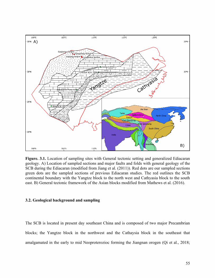
Figure. 3.1. Location of sampling sites with General tectonic setting and generalized Ediacaran
geology. A) Location of sampled sections and major faults and folds with general geology of the
SCB during the Ediacaran (modified from Jiang et al. (2011)). Red dots are our sampled sections
green dots are the sampled sections of previous Ediacaran studies. The red outlines the SCB
continental boundary with the Yangtze block to the north west and Cathyasia block to the south
east. B) General tectonic framework of the Asian blocks modified from Mathews et al. (2016).
3.2. Geological background and sampling
The SCB is located in present day southeast China and is composed of two major Precambrian
blocks; the Yangtze block in the northwest and the Cathaysia block in the southeast that
amalgamated in the early to mid Neoproterozioc forming the Jiangnan orogen (Qi et al., 2018;
56
Cawood et al., 2018 and references therein). The SCB is bounded in the north to the North China
Block by the Qinling-Dabie-Sulu orogen, in the east bounded to the Sogpan-Garze terran along
the Longmentshan fault, and in the south to Indochina along the Ailaoshan-Song Ma suture zone
(Cawood et al., 2018; Domeier, 2018).
The depositional environment throughout the Ediacaran on SCB has been interpreted as a
shallow marine environment deposited along a passive margin with the depositional facies
shallowing from the south east on the Cathaysia block to the north west on the Yangtze block
(Jiang et al., 2011). The lithofacies are dominated by many transgressive and regressive
sequences which has preserved many Ediacaran biota (Jiang et al., 2011).
Our paleomagnetic study was conducted in four sections on the north western margin of the SCB
in the southern portion of the Shaanxi Province (Figure 3.1). The Gangchang (32.89° N, 106.72°
E) and the GaoJiaShan (32.97° N, 106.46° E) sections, were brought to surface the folding and
thrusting of the Longmen-Shen suture. The LiangHeKuo (32.39° N, 107.99° E), and Xiaoyang
(32.55° N, 107.95° E) sections, were brought to surface by the East Qingling thrust system.
In our study locality the SCB for the Ediacaran formations are composed of the Doushantuo
formation overlain by the Dengying formation. The age constraints on the Doushantuo formation
are from two ash beds just above the cap dolostone of the Doushantuo formation (635 Ma) and
an ash bed at the top of the Doushantuo formation (551.1) (Condon et al., 2005).
57
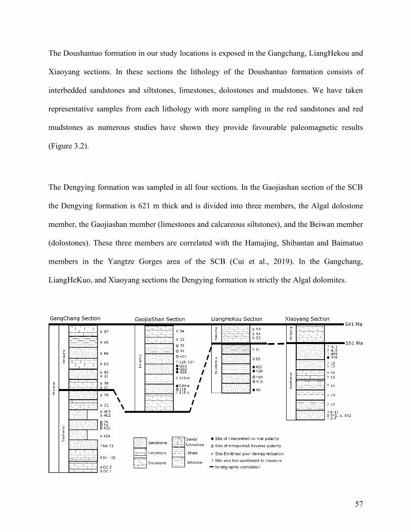
The Doushantuo formation in our study locations is exposed in the Gangchang, LiangHekou and
Xiaoyang sections. In these sections the lithology of the Doushantuo formation consists of
interbedded sandstones and siltstones, limestones, dolostones and mudstones. We have taken
representative samples from each lithology with more sampling in the red sandstones and red
mudstones as numerous studies have shown they provide favourable paleomagnetic results
(Figure 3.2).
The Dengying formation was sampled in all four sections. In the Gaojiashan section of the SCB
the Dengying formation is 621 m thick and is divided into three members, the Algal dolostone
member, the Gaojiashan member (limestones and calcareous siltstones), and the Beiwan member
(dolostones). These three members are correlated with the Hamajing, Shibantan and Baimatuo
members in the Yangtze Gorges area of the SCB (Cui et al., 2019). In the Gangchang,
LiangHeKuo, and Xiaoyang sections the Dengying formation is strictly the Algal dolomites.
58
Figure. 3.2. Schematic stratigraphy of each sample site in each section and formation. The open
circles are reverse polarity and the black circles are normal polarity sites, the X’s indicate sites
which exhibit poor magnetizations or absence of readable remnant magnetization, the ? are sites
that were composed by the weathered rocks that produced unreliable results.
3.3. Methods
We took standard paleomagnetic drilling cores with a gasoline powered drill and oriented hand
blocks. Hand blocks were taken in stratigraphic coordinates, registering the dip and azimuth of
the dip, when the sediments were weathered and drilling was not possible. Cores and hand
blocks were oriented in the field using a magnetic compass and a sun compass when weather
permitted. There was no significant difference between the two measurements. The drilled cores
were 2.2 cm in diameter and cut into samples with heights varying from 1 cm to 2.5 cm. The
hand blocks were drilled and cut into cylindrical samples or were cut into cubic samples to a
maximum size of 2.2x2.2x2.2 cm3.
All measurements took place in three laboratories, 90% in the Laboratory of Paleomagnetism
and Petromagnetism of the University of Alberta (Edmonton, Canada), and pilot samples were
measured at the Ivar Giaever Geomagnetic Laboratory (University of Oslo, Norway) and
Paleomagnetic Laboratory of the Northwest University (Xi’an, China). Measurements were
performed with a 2G cryogenic magnetometer in all three labs and demagnetizations were
carried out in the permalloy shielded room of the University of Alberta with ambient magnetic
field less than 10 nT and MMLFC shielded room at the University of Oslo with ambient
magnetic field 100 nT. Prior to measurements samples were stored in μ-metal shielded chamber
or room. Thermal demagnetizations were carried out using the TD-48SC ASC thermal

59
demagnetizer and alternating field demagnetization was carried out using the 2G degaussing
system. There was no systematic difference observed in results from the three laboratories.
Preliminary samples from each site were demagnetized at steps of 25 °C or 2 to 10 mT (AF)
until the measurements became unstable or sporadic indicating mineralogical changes or
spurious fields were acquired. The mineralogical changes were monitored by measurements of
magnetic susceptibility after every temperature step for the pilot samples. Paleomagnetic
directions are determined using principal component analysis (PCA) (Kirschvink, 1980) and
constrained great circles (GC) fitting (McFadden and McElhinny, 1998). Paleomagnetic data was
analyzed using the software packages PMGSC (Enkin, 1994) and PaleoMac (Congné. 2003).
To constrain the magnetic carrying minerals in our samples we performed temperature dependent
magnetic susceptibility, IRM, and hysteresis measurements. Detailed rock magnetic
measurements were performed on sites that represented primary magnetizations. Magnetic
susceptibility measurements were carried out in an AGICO MFK1-FA Kappabridge with CS-4
furnace and processed with Cureval-8 software (Agico Inc). Hysteresis and IRM measurements
were taken with a Lake Shore PMC MicroMag 3900 VSM.
3.4. Rock Magnetic Analysis
Rock magnetic studies were carried out only on sites in which demagnetizations were successful.
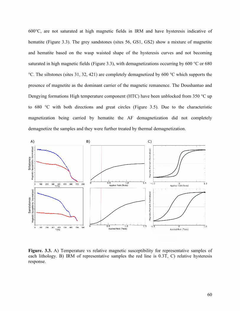
We measured magnetic susceptibility versus temperature, IRM and hysteresis (Figure 3.3). The
red sandstones (sites 74, 75, 405, 418, 419, 420) show a change in magnetic susceptibility above
60
600°C, are not saturated at high magnetic fields in IRM and have hysteresis indicative of
hematite (Figure 3.3). The grey sandstones (sites 56, GS1, GS2) show a mixture of magnetite
and hematite based on the wasp waisted shape of the hysteresis curves and not becoming
saturated in high magnetic fields (Figure 3.3), with demagnetizations occurring by 600 °C or 680
°C. The siltstones (sites 31, 32, 421) are completely demagnetized by 600 °C which supports the
presence of magnetite as the dominant carrier of the magnetic remanence. The Doushantuo and
Dengying formations High temperature component (HTC) have been unblocked from 350 °C up
to 680 °C with both directions and great circles (Figure 3.5). Due to the characteristic
magnetization being carried by hematite the AF demagnetization did not completely
demagnetize the samples and they were further treated by thermal demagnetization.
Figure. 3.3. A) Temperature vs relative magnetic susceptibility for representative samples of
each lithology. B) IRM of representative samples the red line is 0.3T, C) relative hysteresis
response.
61
3.5. Paleomagnetic analysis
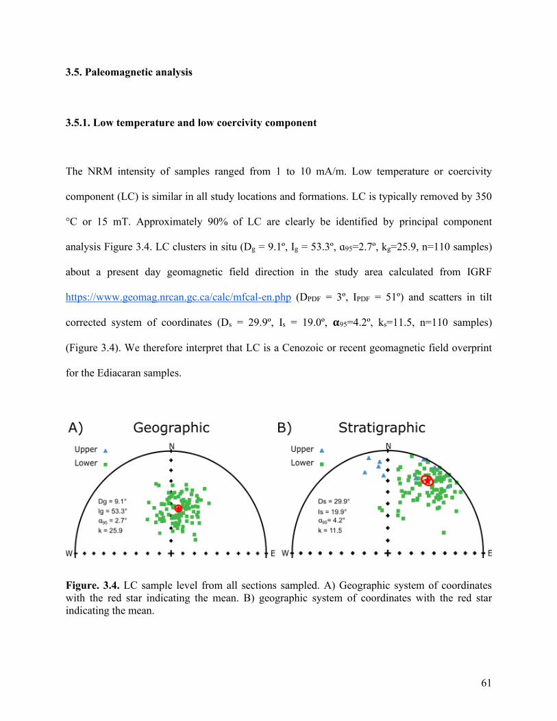
3.5.1. Low temperature and low coercivity component
The NRM intensity of samples ranged from 1 to 10 mA/m. Low temperature or coercivity
component (LC) is similar in all study locations and formations. LC is typically removed by 350
°C or 15 mT. Approximately 90% of LC are clearly be identified by principal component
analysis Figure 3.4. LC clusters in situ (Dg = 9.1º, Ig = 53.3º, ɑ95=2.7º, kg=25.9, n=110 samples)
about a present day geomagnetic field direction in the study area calculated from IGRF
https://www.geomag.nrcan.gc.ca/calc/mfcal-en.php (DPDF = 3º, IPDF = 51º) and scatters in tilt
corrected system of coordinates (Ds = 29.9º, Is = 19.0º, 𝛂95=4.2º, ks=11.5, n=110 samples)
(Figure 3.4). We therefore interpret that LC is a Cenozoic or recent geomagnetic field overprint
for the Ediacaran samples.
Figure. 3.4. LC sample level from all sections sampled. A) Geographic system of coordinates
with the red star indicating the mean. B) geographic system of coordinates with the red star
indicating the mean.
62
3.5.2. High Temperature Component (HTC)
3.5.2.1. Doushantuo formation (Ediacaran, 635-551.1 Ma)
The HTC is isolated above 450°C and has two polarities with the normal polarity preserved in
the grey sandstones and blue siltstones and the reverse polarity in the red sandstone and siltstone
beds. Both the normal polarity and reverse polarities are represented by great circles and PCA
directions. The sites that preserve HTC are stratigraphically located at the top of the Doushantuo
formation (Figure 3.2). The LiangHeKuo section shows two polarities with south west cluster for
and north east cluster (Fig. 3.5, Table 3.1). The Xiaoyang section shows a north east cluster with
a single polarity and the GangChang section only shows a single polarity clustering in the north
west in stratigraphic coordinates.
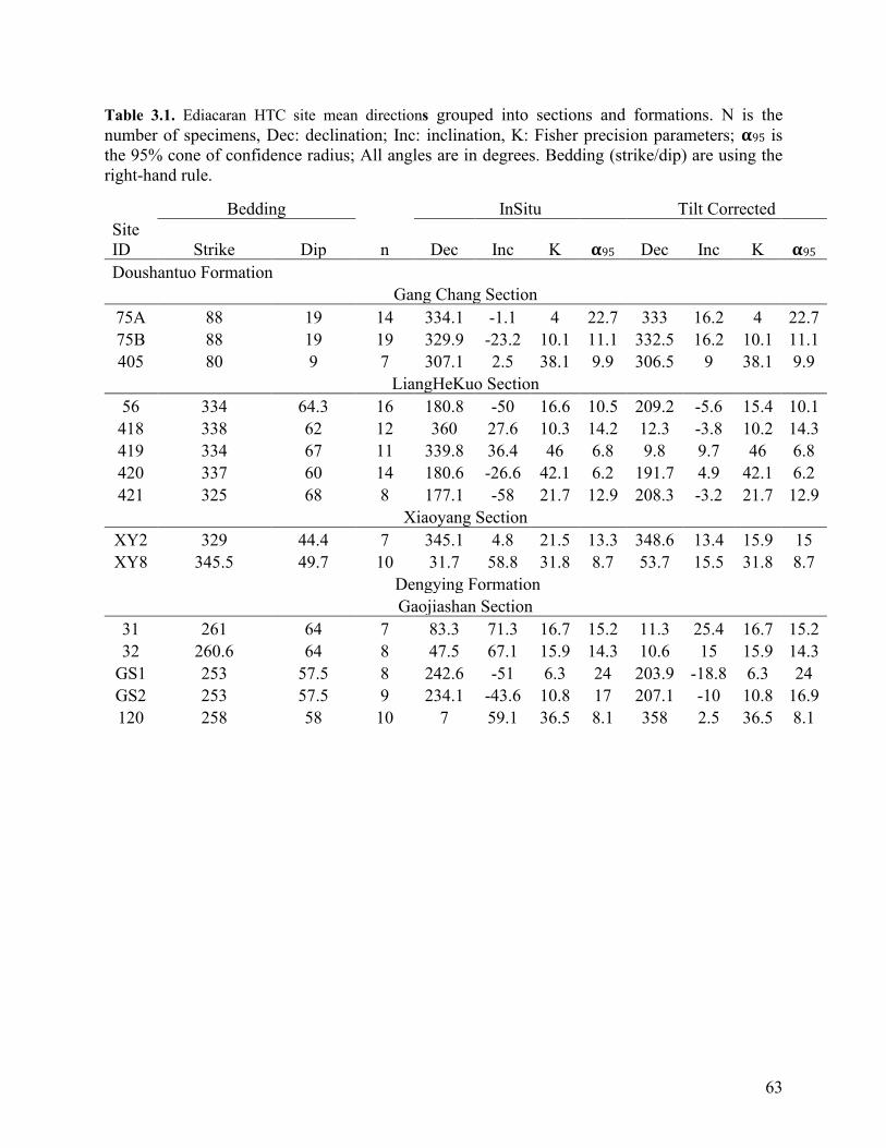
63
Table 3.1. Ediacaran HTC site mean directions grouped into sections and formations. N is the
number of specimens, Dec: declination; Inc: inclination, K: Fisher precision parameters; 𝛂95 is
the 95% cone of confidence radius; All angles are in degrees. Bedding (strike/dip) are using the
right-hand rule.
Bedding InSitu Tilt Corrected
Site
ID Strike Dip n Dec Inc K 𝛂95 Dec Inc K 𝛂95
Doushantuo Formation
Gang Chang Section
75A 88 19 14 334.1 -1.1 4 22.7 333 16.2 4 22.7
75B 88 19 19 329.9 -23.2 10.1 11.1 332.5 16.2 10.1 11.1
405 80 9 7 307.1 2.5 38.1 9.9 306.5 9 38.1 9.9
LiangHeKuo Section
56 334 64.3 16 180.8 -50 16.6 10.5 209.2 -5.6 15.4 10.1
418 338 62 12 360 27.6 10.3 14.2 12.3 -3.8 10.2 14.3
419 334 67 11 339.8 36.4 46 6.8 9.8 9.7 46 6.8
420 337 60 14 180.6 -26.6 42.1 6.2 191.7 4.9 42.1 6.2
421 325 68 8 177.1 -58 21.7 12.9 208.3 -3.2 21.7 12.9
Xiaoyang Section
XY2 329 44.4 7 345.1 4.8 21.5 13.3 348.6 13.4 15.9 15
XY8 345.5 49.7 10 31.7 58.8 31.8 8.7 53.7 15.5 31.8 8.7
Dengying Formation
Gaojiashan Section
31 261 64 7 83.3 71.3 16.7 15.2 11.3 25.4 16.7 15.2
32 260.6 64 8 47.5 67.1 15.9 14.3 10.6 15 15.9 14.3
GS1 253 57.5 8 242.6 -51 6.3 24 203.9 -18.8 6.3 24
GS2 253 57.5 9 234.1 -43.6 10.8 17 207.1 -10 10.8 16.9
120 258 58 10 7 59.1 36.5 8.1 358 2.5 36.5 8.1
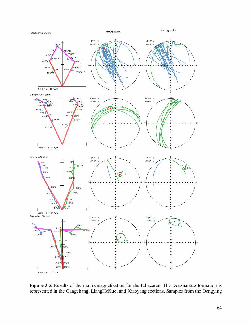
64
Figure 3.5. Results of thermal demagnetization for the Ediacaran. The Doushantuo formation is
represented in the Gangchang, LiangHeKuo, and Xiaoyang sections. Samples from the Dengying
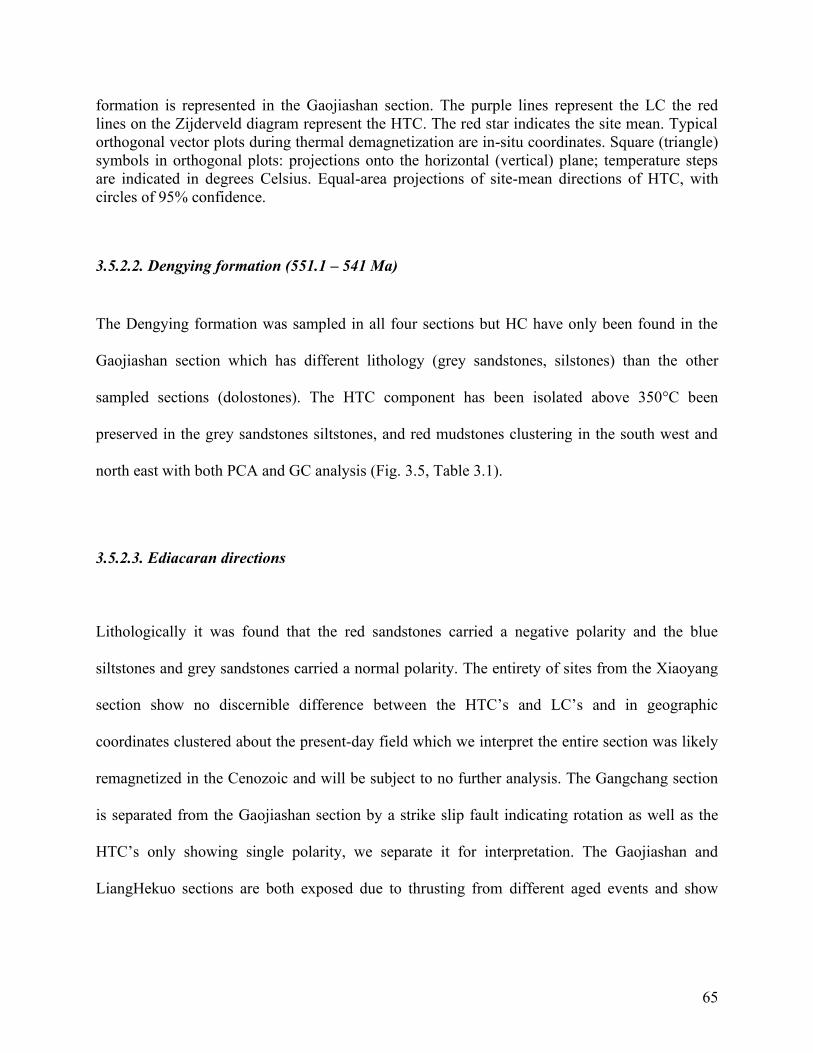
65
formation is represented in the Gaojiashan section. The purple lines represent the LC the red
lines on the Zijderveld diagram represent the HTC. The red star indicates the site mean. Typical
orthogonal vector plots during thermal demagnetization are in-situ coordinates. Square (triangle)
symbols in orthogonal plots: projections onto the horizontal (vertical) plane; temperature steps
are indicated in degrees Celsius. Equal-area projections of site-mean directions of HTC, with
circles of 95% confidence.
3.5.2.2. Dengying formation (551.1 – 541 Ma)
The Dengying formation was sampled in all four sections but HC have only been found in the
Gaojiashan section which has different lithology (grey sandstones, silstones) than the other
sampled sections (dolostones). The HTC component has been isolated above 350°C been
preserved in the grey sandstones siltstones, and red mudstones clustering in the south west and
north east with both PCA and GC analysis (Fig. 3.5, Table 3.1).
3.5.2.3. Ediacaran directions
Lithologically it was found that the red sandstones carried a negative polarity and the blue
siltstones and grey sandstones carried a normal polarity. The entirety of sites from the Xiaoyang
section show no discernible difference between the HTC’s and LC’s and in geographic
coordinates clustered about the present-day field which we interpret the entire section was likely
remagnetized in the Cenozoic and will be subject to no further analysis. The Gangchang section
is separated from the Gaojiashan section by a strike slip fault indicating rotation as well as the
HTC’s only showing single polarity, we separate it for interpretation. The Gaojiashan and
LiangHekuo sections are both exposed due to thrusting from different aged events and show
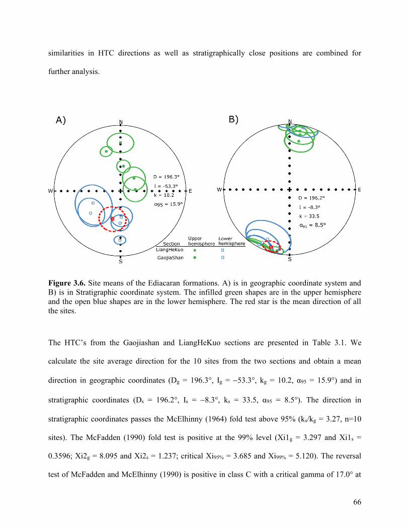
66
similarities in HTC directions as well as stratigraphically close positions are combined for
further analysis.
Figure 3.6. Site means of the Ediacaran formations. A) is in geographic coordinate system and
B) is in Stratigraphic coordinate system. The infilled green shapes are in the upper hemisphere
and the open blue shapes are in the lower hemisphere. The red star is the mean direction of all
the sites.
The HTC’s from the Gaojiashan and LiangHeKuo sections are presented in Table 3.1. We
calculate the site average direction for the 10 sites from the two sections and obtain a mean
direction in geographic coordinates (Dg = 196.3°, Ig = −53.3°, kg = 10.2, α95 = 15.9°) and in
stratigraphic coordinates (Ds = 196.2°, Is = −8.3°, ks = 33.5, α95 = 8.5°). The direction in
stratigraphic coordinates passes the McElhinny (1964) fold test above 95% (ks/kg = 3.27, n=10
sites). The McFadden (1990) fold test is positive at the 99% level (Xi1g = 3.297 and Xi1s =
0.3596; Xi2g = 8.095 and Xi2s = 1.237; critical Xi95% = 3.685 and Xi99% = 5.120). The reversal
test of McFadden and McElhinny (1990) is positive in class C with a critical gamma of 17.0° at
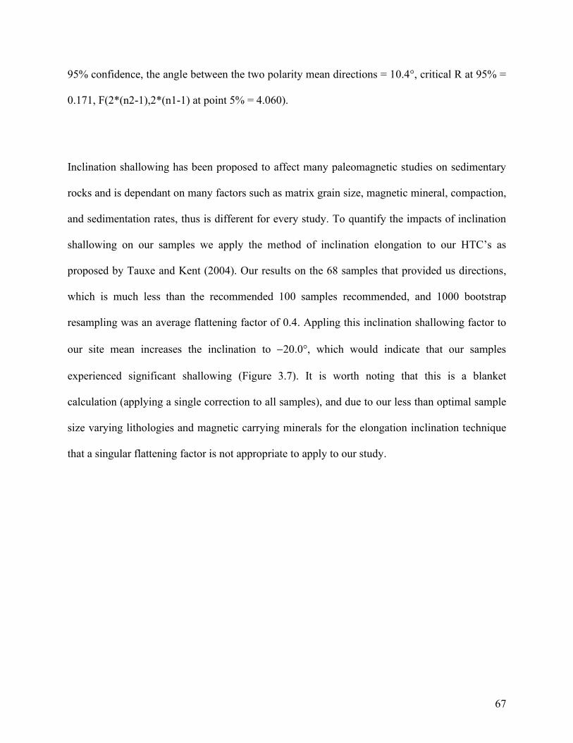
67
95% confidence, the angle between the two polarity mean directions = 10.4°, critical R at 95% =
0.171, F(2*(n2-1),2*(n1-1) at point 5% = 4.060).
Inclination shallowing has been proposed to affect many paleomagnetic studies on sedimentary
rocks and is dependant on many factors such as matrix grain size, magnetic mineral, compaction,
and sedimentation rates, thus is different for every study. To quantify the impacts of inclination
shallowing on our samples we apply the method of inclination elongation to our HTC’s as
proposed by Tauxe and Kent (2004). Our results on the 68 samples that provided us directions,
which is much less than the recommended 100 samples recommended, and 1000 bootstrap
resampling was an average flattening factor of 0.4. Appling this inclination shallowing factor to
our site mean increases the inclination to −20.0°, which would indicate that our samples
experienced significant shallowing (Figure 3.7). It is worth noting that this is a blanket
calculation (applying a single correction to all samples), and due to our less than optimal sample
size varying lithologies and magnetic carrying minerals for the elongation inclination technique
that a singular flattening factor is not appropriate to apply to our study.
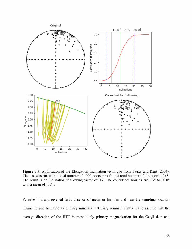
68
Figure 3.7. Application of the Elongation Inclination technique from Tauxe and Kent (2004).
The test was run with a total number of 1000 bootstraps from a total number of directions of 68.
The result is an inclination shallowing factor of 0.4. The confidence bounds are 2.7° to 20.0°
with a mean of 11.4°.
Positive fold and reversal tests, absence of metamorphism in and near the sampling locality,
magnetite and hematite as primary minerals that carry remnant enable us to assume that the
average direction of the HTC is most likely primary magnetization for the Gaojiashan and
69
LiangHeKuo sections. A new paleomagnetic pole was calculated for the tilt-corrected system of
coordinates 57.9 °S and 75.0 °E (dm = 8.6°, dp = 4.3°) with a paleolatitude of 4.2 °S ± 4.3°
(Figure 3.8 pole 1). This new pole does not resemble any younger paleomagnetic pole.
From the Gangchang section we get a section mean of Dg = 145.4°, Ig = 9.1°, kg = 22.7, ɑ95 =
19.7° in geographic coordinates and Ds = 146.1°, Is = −5.5°, ks = 25.6, ɑ95 = 18.5°. There is not a
large dip for the Gangchang section which explains why the geographic and stratigraphic
coordinates are similar. Using the stratigraphic coordinate system, we produce a paleomagnetic
pole of 46.4 °S and 160.6 °E (dp = 18.6°, dm = 9.3°) with a paleolatitude of 2.8 °S ± 9.3° (Figure
3.8 Pole 2). This pole only has one polarity, and no fold test but it does not resemble any younger
paleopoles in either geographic or stratigraphic systems of coordinates (Figure 3.8 pole 2).
3.6. Discussion
3.6.1. Comparison of paleomagnetic poles
We obtain two poles for the Ediacaran. Pole 1 is sampled from the LiangHeKuo and Gaojiashan
sections and pole 2 is from the Gangchang section. Pole 1 has a quality factor of 7 based on Van
der Voo (1990) criteria, this includes positive fold and reversal tests, no resemblance to younger
poles, adequate demagnetization with PCA, the age is well dated within 20 Ma (551 Ma), and
sufficient samples with a confidence cone less than 16°. We interpret pole 1 as the primary
magnetization and present the first reliable Ediacaran pole for the SCB. Pole 2 only has one
polarity and has no fold test. We plot the two poles in Figure 3.8. We find that the rotation angle
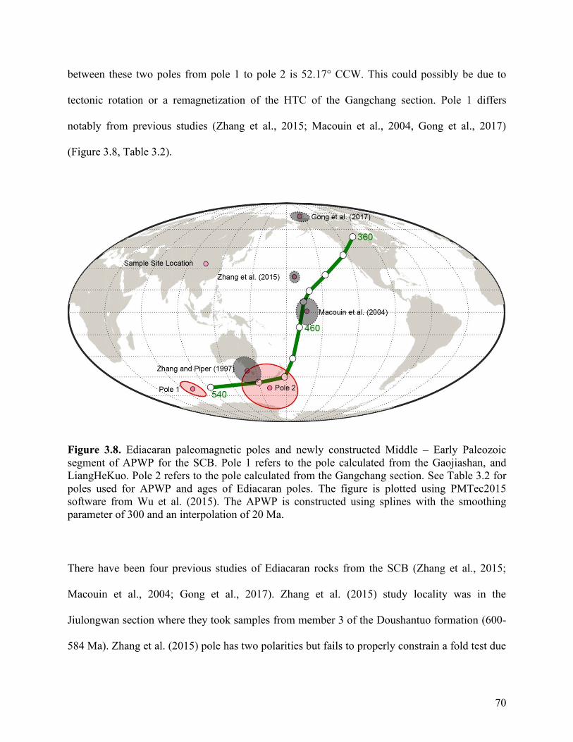
70
between these two poles from pole 1 to pole 2 is 52.17° CCW. This could possibly be due to
tectonic rotation or a remagnetization of the HTC of the Gangchang section. Pole 1 differs
notably from previous studies (Zhang et al., 2015; Macouin et al., 2004, Gong et al., 2017)
(Figure 3.8, Table 3.2).
Figure 3.8. Ediacaran paleomagnetic poles and newly constructed Middle – Early Paleozoic
segment of APWP for the SCB. Pole 1 refers to the pole calculated from the Gaojiashan, and
LiangHeKuo. Pole 2 refers to the pole calculated from the Gangchang section. See Table 3.2 for
poles used for APWP and ages of Ediacaran poles. The figure is plotted using PMTec2015
software from Wu et al. (2015). The APWP is constructed using splines with the smoothing
parameter of 300 and an interpolation of 20 Ma.
There have been four previous studies of Ediacaran rocks from the SCB (Zhang et al., 2015;
Macouin et al., 2004; Gong et al., 2017). Zhang et al. (2015) study locality was in the
Jiulongwan section where they took samples from member 3 of the Doushantuo formation (600-
584 Ma). Zhang et al. (2015) pole has two polarities but fails to properly constrain a fold test due
71
to the shallow dipping nature of the fold limbs sampled. Zhang et al. (2015) pole resembles the
Triassic portion of the APWP. Macouin et al. (2004) study was from member 3 of the
Doushantuo formation (600-584 Ma) in the Shiman section of the Hunan province that was
folded in the Jurassic. They present positive fold tests though they report only a single polarity.
Their pole strongly resembles the Silurian pole of the SCB (Table 3.2). Gong et al. (2017)
reported the Dongdahe section Member three and suggested a possibility of Mesozoic
remagnetization due to the late Mesozoic Yanshanian orogeny in the Cretaceous due to its single
polarity and resemblance to the Cenozoic paleomagnetic poles. Zhang and Piper (1997) proposed
three poles from rocks at the top of the Nantuo formation dated at the end of the Cryogenian and
the bottom of the Doushantuo formation, dated at the beginning of the Ediacaran from Wong’an,
South China. Their Ediacaran pole provides only a single polarity, has no fold test and resembles
close to more recently published Cambrian poles and pole 2 from the Gangchang section.
We conclude that other poles published for Ediacaran rocks do not meet the full criteria to be
considered primary magnetization due to lack of reliability tests and similarities to younger
paleomagnetic poles, these poles should not be used for constructing the APWP or plate tectonic
reconstructions. In order to create a new APWP for the SCB we use the compilation of middle to
early Paleozoic poles from Domeier (2018), with the addition of our new Ediacaran pole 1
(Table 3.2). To calculate the APWP we use the PMtech 2015 software (Wu et al., 2015) using a
spherical spline with a smoothing parameter of 300 and an interpolation of 20 Ma (Figure 3.8).
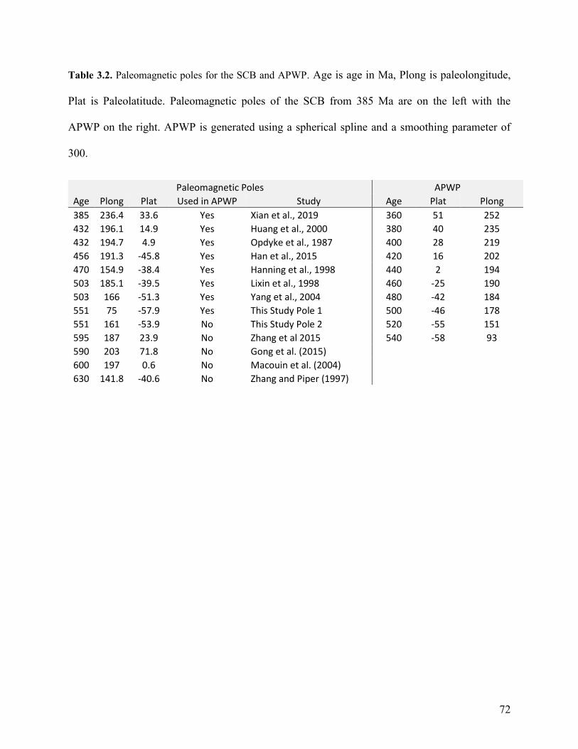
72
Table 3.2. Paleomagnetic poles for the SCB and APWP. Age is age in Ma, Plong is paleolongitude,
Plat is Paleolatitude. Paleomagnetic poles of the SCB from 385 Ma are on the left with the
APWP on the right. APWP is generated using a spherical spline and a smoothing parameter of
300.
Paleomagnetic Poles APWP
Age Plong Plat Used in APWP Study Age Plat Plong
385 236.4 33.6 Yes Xian et al., 2019 360 51 252
432 196.1 14.9 Yes Huang et al., 2000 380 40 235
432 194.7 4.9 Yes Opdyke et al., 1987 400 28 219
456 191.3 -45.8 Yes Han et al., 2015 420 16 202
470 154.9 -38.4 Yes Hanning et al., 1998 440 2 194
503 185.1 -39.5 Yes Lixin et al., 1998 460 -25 190
503 166 -51.3 Yes Yang et al., 2004 480 -42 184
551 75 -57.9 Yes This Study Pole 1 500 -46 178
551 161 -53.9 No This Study Pole 2 520 -55 151
595 187 23.9 No Zhang et al 2015 540 -58 93
590 203 71.8 No Gong et al. (2015)
600 197 0.6 No Macouin et al. (2004)
630 141.8 -40.6 No Zhang and Piper (1997)
73
3.7. Paleogeographic Reconstruction
The difficult debate as to the location of the SCB and its relationship to India and Australia is
coming closer to a consensus. Interpretations of paleontological data place the SCB to the
western margin of Gondwana (Cocks and Torsvik, 2013; Domeier, 2018) and references
therein). Qi et al. (2018) suggest that detrital zircons are derived from the India block throughout
the Ediacaran and infer that the SCB was in close proximity of India throughout the Ediacaran.
With our new well dated and reliable paleomagnetic pole we have paleolatitude and orientation
constraint on the SCB at the end of the Ediacaran. We can confidently place the SCB off the
northern portion of India as an integral part of Gondwana (Figure 3.9). The southern edge of the
SCB in the present-day coordinates was facing north.
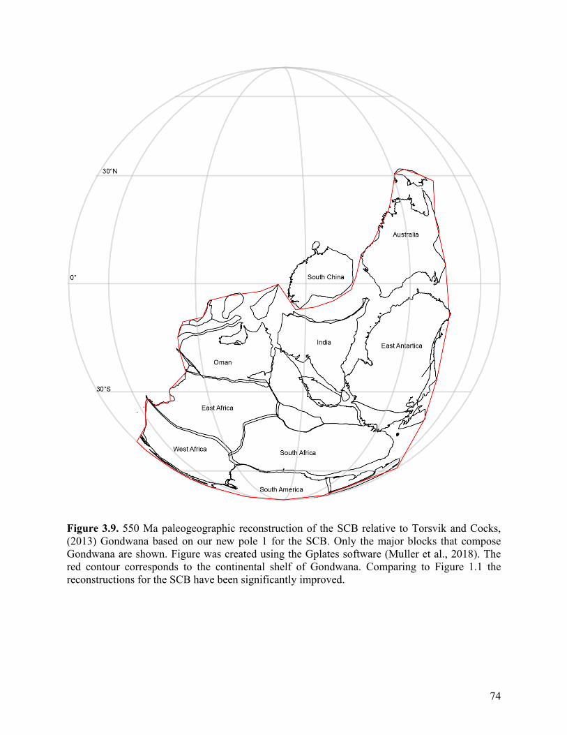
74
Figure 3.9. 550 Ma paleogeographic reconstruction of the SCB relative to Torsvik and Cocks,
(2013) Gondwana based on our new pole 1 for the SCB. Only the major blocks that compose
Gondwana are shown. Figure was created using the Gplates software (Muller et al., 2018). The
red contour corresponds to the continental shelf of Gondwana. Comparing to Figure 1.1 the
reconstructions for the SCB have been significantly improved.
75
3.8. Conclusions
Our study provides the first reliable paleomagnetic pole for the South China Block for the late
Ediacaran. The reliability of this pole is solidified by well constrained age, 95 less than 16,
PCA of directions, absence of significant metamorphism, passing the fold and reversal tests, and
lack of resemblance to any younger paleomagnetic poles, passing all seven criteria outlined in
Van der Voo (1990). Pole 1 differs significantly from previously published Ediacaran. Due to the
depositional environment indicating a passive margin (Jiang et al., 2011), sedimentary source
rocks for the SCB derived from India (Qi et al., 2018), combined with our paleomagnetic results
we place the SCB off the northern portion of India and west of Australia as part of east
Gondwana at the end of the Ediacaran. The present day south of the SCB faces north in the
Ediacaran reconstruction.
The new paleogeographic reconstruction for the SCB indicates that it was a significant member
of Gondwana to which three of the four continents that have the formations that the Shuram
Wonoka excursion (SWE) is found. With the final amalgamation of Gondwana occurring after
the deposition of the formations that host the SWE, this could indicate that the SWE occurred
during final amalgamation of Gondwana. As the proximity of Laurentia to Gondwana is still
debated that hypothesis may not be resolved.
76
Chapter 4: Conclusions
In conclusion this thesis has crucial implications on modelling magnetic anomalies (Chapter 2)
and Ediacaran paleogeography (Chapter 3). First by providing the corrected algorithm for fast
modelling of irregular 2-dimensional bodies along with computational software which is
available at the website www.ualberta.ca/~vadim/software.htm and second by providing the first
reliable paleomagnetic pole for the SCB at the Ediacaran Cambrian transition.
Upon close inspection of the derivation of equations originally published by Talwani and
Heirtzler (1964), erroneous definitions were used leading to incorrect solutions for forward
modeling of particular 2D geometries; this is outlined in chapter 2. These errors if made by
themselves produce large discrepancies in the forward modelling of the magnetic field but if all
made together then can produce the correct answer. It is unclear when these errors will cause
instabilities and incorrect anomalies. We present a new algorithm and transparency in derivation,
that has been proofed several times and produces stable answers to which we recommend that it
be used for future modelling and for verification of old models. For user friendly implementation
of this algorithm we created a Matlab GUI and executable for those who do not have Matlab.
Features of our software include; calculation of remnant magnetization direction if the
paleomagnetic pole is known, single calculation using both induced and remnant magnetizations,
importing of data from processing software’s in either profile of gridded data, and exporting
models. To further the software for academic use additions of error analysis and interactions of
model fitting to determine a best fit curve can be obtained using least squares polynomial fits.
77
We provide a new paleomagnetic pole for the Ediacaran of the SCB that passes all reliability
tests for primary magnetization, which is the first from the SCB. With our new Ediacaran
paleomagnetic pole we are finally able to construct the APWP for the SCB into the Ediacaran.
We are also able to produce the first constrained paleogeographic reconstruction for the SCB at
the Ediacaran Cambrian boundary. In this new construction we place the SCB along the eastern
margin of Gondwana connected to India. This new reconstruction allows to constraint future
modelling of climate, environment and geochemical events prior to the Cambrian explosion. To
further understand the final amalgamation of Gondwana throughout the Ediacaran the next step
would be to combine the Neoproterozoic paleomagnetic poles of the SCB and India and compare
them to the APWP of the rest of the Gondwana continents to determine the final assemblage of
the supercontinent.
The next largest of the Asian blocks after the SCB is the North China Block (NCB), also lacks
paleomagnetic data in the Ediacaran which has led to a significant number of unconstrained
models (Figure 1.1, Figure 3.9) (Li et al., 2018; Mckenzie et al., 2011; Cocks and Torsvik,
2013). Cambrian trilobite similarity has led to the consensus that the North China Block was in
some proximity of the SCB though that is the only constraint on its location in the Ediacaran
(Mckenzie et al., 2011), therefore paleomagnetic study is necessary to constrain the position of
the NCB. A paleomagnetic study of the NCB will require much the same style of sampling and
approach as was taken in our study of the SCB as there has been no previous paleomagnetic
studies on Ediacaran rocks. This will require new field work and systematic measurements of
each lithology to determine if there is primary remnant magnetization present.
78
References
Cawood, P. A., Zhao, G., Yao, J., Wang, W., Xu, Y., & Wang, Y. (2018). Reconstructing South
China in phanerozoic and precambrian supercontinents. Earth-Science Reviews, 186, 173-194.
Charvet, J. (2013). The Neoproterozoic–early Paleozoic tectonic evolution of the South China
Block: an overview. Journal of Asian Earth Sciences, 74, 198-209.
Cocks, L. R. M., & Torsvik, T. H. (2013). The dynamic evolution of the Palaeozoic geography
of eastern Asia. Earth-Science Reviews, 117, 40-79.
Cogné, J.P., 2003. PaleoMac: a Macintosh™ application for treating paleomagnetic data and
making plate reconstructions. Geochemistry, Geophysics, Geosystems, 4(1).
Condon, D., Zhu, M., Bowring, S., Wang, W., Yang, A., & Jin, Y. (2005). U-Pb ages from the
neoproterozoic Doushantuo Formation, China. Science, 308(5718), 95-98.
Cui, H., Xiao, S., Cai, Y., Peek, S., Plummer, R. E., & Kaufman, A. J. (2019). Sedimentology
and chemostratigraphy of the terminal Ediacaran Dengying Formation at the Gaojiashan section,
South China. Geological Magazine, 1-25.
Driscoll, P. E., & Evans, D. A. (2016). Frequency of Proterozoic geomagnetic superchrons.
Earth and Planetary Science Letters, 437, 9-14.
Domeier, M. (2018). Early Paleozoic tectonics of Asia: Towards a full-plate model. In
Geoscience Frontiers (Vol. 9, Issue 3, pp. 789–862).
Enkin, R.J., 1994. A computer program package for analysis and presentation of paleomagnetic
data. Pacific Geoscience Centre, Geological Survey of Canada, 16.
Fike, D. A., Grotzinger, J. P., Pratt, L. M., & Summons, R. E. (2006). Oxidation of the Ediacaran
ocean. nature,444(7120), 744.
Gong, Z., Kodama, K. P., & Li, Y. X. (2017). Rock magnetic cyclostratigraphy of the
Doushantuo Formation, South China and its implications for the duration of the Shuram carbon
isotope excursion. Precambrian Research, 289, 62-74.
Grotzinger, J. P., Fike, D. A., & Fischer, W. W. (2011). Enigmatic origin of the largest-known
carbon isotope excursion in Earth's history. Nature Geoscience, 4(5), 285.
Hoffman, P. F., & Schrag, D. P. (2002). The snowball Earth hypothesis: testing the limits of
global change. Terra nova, 14(3), 129-155.
Jeshvaghani, M. S., & Darijani, M. (2014). Two-dimensional geomagnetic forward modeling
using adaptive finite element method and investigation of the topographic effect. Journal of
Applied Geophysics, 105, 169-179.
79
Jiang, G., Shi, X., Zhang, S., Wang, Y., & Xiao, S. (2011). Stratigraphy and paleogeography of
the Ediacaran Doushantuo Formation (ca. 635–551 Ma) in south China. Gondwana Research,
19(4), 831-849.
Jiao, W., Li, Y. X., Yang, Z., & Liu, J. (2019). A Widespread Early Mesozoic Remagnetization
in South China. Journal of Geophysical Research: Solid Earth, 124(1), 88-103.
Kostrov, N. P. (2007). Calculation of magnetic anomalies caused by 2D bodies of arbitrary shape
with consideration of demagnetization. Geophysical prospecting, 55(1), 91-115.
Lelievre, P.G., & Oldenburg, D.W. (2006). Magnetic forward modelling and inversion for high
susceptibility. Geophysical Journal International, 166 (1), 76-90.
Li, S., Zhao, S., Liu, X., Cao, H., Yu, S., Li, X., ... & Suo, Y. (2018). Closure of the Proto-Tethys
Ocean and Early Paleozoic amalgamation of microcontinental blocks in East Asia. Earth-Science
Reviews, 186, 37-75.
Kirschvink, J. L. (1980). The least-squares line and plane and the analysis of palaeomagnetic
data. Geophysical Journal International, 62(3), 699-718.
Macouin, M., Besse, J., Ader, M., Gilder, S., Yang, Z., Sun, Z., & Agrinier, P. (2004). Combined
paleomagnetic and isotopic data from the Doushantuo carbonates, South China: implications for
the “snowball Earth” hypothesis. Earth and Planetary Science Letters, 224(3-4), 387-398.
Matthews, K. J., Maloney, K. T., Zahirovic, S., Williams, S. E., Seton, M., & Mueller, R. D.
(2016). Global plate boundary evolution and kinematics since the late Paleozoic. Global and
Planetary Change, 146, 226-250.
McElhinny, M. W., & McFadden, P. L. (1998). The magnetic field of the earth: paleomagnetism,
the core, and the deep mantle (Vol. 63). Academic Press.
McFadden, K. A., Huang, J., Chu, X., Jiang, G., Kaufman, A. J., Zhou, C., ... & Xiao, S. (2008).
Pulsed oxidation and biological evolution in the Ediacaran Doushantuo Formation. Proceedings
of the National Academy of Sciences, 105(9), 3197-3202.
McKenzie, N. R., Hughes, N. C., Myrow, P. M., Choi, D. K., & Park, T. Y. (2011). Trilobites
and zircons link north China with the eastern Himalaya during the Cambrian. Geology, 39(6),
591-594.
Müller, R. D., Cannon, J., Qin, X., Watson, R. J., Gurnis, M., Williams, S., ... & Zahirovic, S.
(2018). GPlates: Building a virtual Earth through deep time. Geochemistry, Geophysics,
Geosystems, 19(7), 2243-2261.
Olson, P., Landeau, M., Reynolds, E., True dipole wander, Geophysical Journal International,
Volume 215, Issue 3, 1 December 2018, Pages 1523–1529, https://doi.org/10.1093/gji/ggy349
80
Qi, L., Xu, Y., Cawood, P. A., & Du, Y. (2018). Reconstructing Cryogenian to Ediacaran
successions and paleogeography of the South China Block. Precambrian Research, 314, 452-
467.
Raub, T. D., Kirschvink, J. L., & Evans, D. A. D. (2007). True polar wander: linking deep and
shallow geodynamics to hydro-and bio-spheric hypotheses. Treatise on geophysics, 5, 565-589.
Talwani, M., & Heirtzler, J. R., 1962. The Mathematical Expression for the Magnetic Anomaly
over a Two-Dimensional Body of Polygonal Cross Section. Lamont Doherty Geol. Obs.
Columbia Univ., Tech. Rep. 6.
Talwani, M., Heirtzler, J. R., 1964. Computation of magnetic anomalies caused by two
dimensional structures of arbitrary shape. Computers in the mineral industries, part 1: Stanford
University publications, Geol. Sciences, 9, 464-480.
Talwani, M. (1965). Computation with the help of a digital computer of magnetic anomalies
caused by bodies of arbitrary shape. Geophysics, 30(5), 797-817.
Tauxe, L., & Kent, D. V. (2004). A simplified statistical model for the geomagnetic field and the
detection of shallow bias in paleomagnetic inclinations: was the ancient magnetic field dipolar?.
Torsvik, T. H., & Cocks, L. R. M. (2013). Gondwana from top to base in space and time.
Gondwana Research, 24(3-4), 999-1030.
Torsvik, T. H., & Cocks, L. R. M. (2017). Earth History and Palaeogeography.
Torsvik, T. H., van der Voo, R., Doubrovine, P. V., Burke, K., Steinberger, B., Ashwal, L. D., ...
& Bull, A. L. (2014). Deep mantle structure as a reference frame for movements in and on the
Earth. Proceedings of the National Academy of Sciences, 111(24), 8735-8740.
Van der Voo, R. (1990). The reliability of paleomagnetic data. Tectonophysics, 184(1), 1-9.
Veevers, J. J. (2004). Gondwanaland from 650–500 Ma assembly through 320 Ma merger in
Pangea to 185–100 Ma breakup: supercontinental tectonics via stratigraphy and radiometric
dating. Earth-Science Reviews, 68(1-2), 1-132.
Williams, G. E., & Schmidt, P. W. (2018). Shuram–Wonoka carbon isotope excursion:
Ediacaran revolution in the world ocean's meridional overturning circulation. Geoscience
Frontiers, 9(2), 391-402.
Won, I. J., & Bevis, M. (1987). Computing the gravitational and magnetic anomalies due to a
polygon: Algorithms and Fortran subroutines. Geophysics, 52(2), 232-238.
Wu, L., Kravchinsky, V. A., & Potter, D. K. (2015). PMTec: A new MATLAB toolbox for
absolute plate motion reconstructions from paleomagnetism. Computers & geosciences, 82, 139-
151.

81
Zhang, S., Li, H., Jiang, G., Evans, D. A., Dong, J., Wu, H., ... & Xiao, Q. (2015). New
paleomagnetic results from the Ediacaran Doushantuo Formation in South China and their
paleogeographic implications. Precambrian Research, 259, 130-142.
Zhang, Q. R., & Piper, J. D. A. (1997). Palaeomagnetic study of Neoproterozoic glacial rocks of
the Yangzi Block: palaeolatitude and configuration of South China in the late Proterozoic
Supercontinent. Precambrian Research, 85(3-4), 173-199.