General rights Copyright and moral rights for the publications made accessible in the public portal are retained by the authors and/or other copyright owners and it is a condition of accessing publications that users recognise and abide by the legal requirements associated with these rights.

• Users may download and print one copy of any publication from the public portal for the purpose of private study or research. • You may not further distribute the material or use it for any profit-making activity or commercial gain • You may freely distribute the URL identifying the publication in the public portal

If you believe that this document breaches copyright please contact us providing details, and we will remove access to the work immediately and investigate your claim.

Downloaded from orbit.dtu.dk on: May 04, 2018

Magnetic signatures of ionospheric and magnetospheric current systems duringgeomagnetic quiet conditions - An overview

Olsen, Nils; Stolle, Claudia

Published in:Space Science Reviews

Link to article, DOI:10.1007/s11214-016-0279-7

Publication date:2017

Document VersionPeer reviewed version

Link back to DTU Orbit

Citation (APA):Olsen, N., & Stolle, C. (2017). Magnetic signatures of ionospheric and magnetospheric current systems duringgeomagnetic quiet conditions - An overview. Space Science Reviews, 206, 5–25. DOI: 10.1007/s11214-016-0279-7

Space Sci. Rev. manuscript No.(will be inserted by the editor)

Magnetic signatures of ionospheric and magnetosphericcurrent systems during geomagnetic quiet conditions -An overview

Nils Olsen · Claudia Stolle

the date of receipt and acceptance should be inserted later

Abstract High-precision magnetic measurements taken by LEO satellites(flying at altitudes between 300 and 800 km) allow for studying the iono-spheric and magnetospheric processes and electric currents that causes onlyweak magnetic signature of a few nanotesla during geomagnetic quiet condi-tions. Of particular importance for this endeavour are multipoint observationsin space, such as provided by the Swarm satellite constellation mission, inorder to better characterize the space-time-structure of the current systems.

Focusing on geomagnetic quiet conditions, we provide an overview of iono-spheric and magnetospheric sources and illustrate their magnetic signatureswith Swarm satellite observations.

Keywords Low Earth-Orbiting Satellites, Geomagnetic Quiet Conditions,Ionospheric and Magnetospheric Currents, Magnetic Field Modeling, Ørsted,CHAMP, Swarm

1 Introduction

Magnetic field measurements taken on ground (e.g. by the network of geomag-netic observatories) or in near-Earth space (by Low-Earth Orbiting satellites)provide a unique opportunity to study the Earth’s interior and its environ-ment. However, what is measured by a magnetometer in space or on groundis the superposition of contributions from various magnetic sources. The mainpart of Earth’s magnetic field is caused by a self-sustaining dynamo operatingin the fluid outer core (at depths greater than 2900 km below surface). Ontop of that there are fields caused by magnetized rocks in the Earth’s crust

N. OlsenDTU Space, Technical University Denmark, Diplomvej 371, DK-2800 Kongens Lyngby, Den-mark, E-mail: nio@space.dtu.dkC. StolleGFZ Potsdam, Telegrafenberg, 14471 Potsdam, Germany

2 Olsen and Stolle

(the so-called crustal or lithospheric field), by electric currents flowing in theionosphere, magnetosphere and oceans, and by currents induced in the Earthby the time-varying external fields. The separation of these various contribu-tions based on observations of the magnetic field requires advanced modellingtechniques (see e.g. Hulot et al. (2015) for an overview).

Determination of models that describe the Earth’s magnetic field at a givenlocation and time is called Geomagnetic modelling. As far as the Earth’s coreand crustal field is concerned, data from geomagnetic quiet days are usuallyselected, to minimize contributions from external (magnetospheric and iono-spheric) sources. But when is “quiet” really quiet – what are proper criteria toselect periods when external sources are weak? How to deal with the remainingpart of external field contributions – what is their impact on models of thecore and crustal field? And in turn: how have high precision magnetic fieldmodels been helpful in describing ionospheric and magnetospheric currentsduring quiet times, and what are still unresolved questions?

This review concerns magnetic field signatures of ionospheric and magne-tospheric current systems during geomagnetic quiet conditions, focusing onphenomena studied with observations taken by high-precision satellite mis-sions. We will discuss the scientific investigations that are possible with thesedata, and present highlights of the obtained results. Building upon our previousreview (Olsen and Stolle 2012) we focus here on research that takes advantageof multi-point magnetic observations in space, as for instance provided by thethree-satellite constellation mission Swarm.

But what characterises “high-precision magnetic satellites” like Ørsted,CHAMP and Swarm? For ground measurements of Earth’s magnetic field itis common to distinguish geomagnetic observatories, where the magnetic fieldvector is measured absolutely, and variometer stations, where only the fieldvariations are measured, which means that the absolute level (the baseline)of the magnetic field is not known (and often vary with time, for instancedue to temperature effects). Variometer data are therefore mainly used forstudying temporal variations of the external field at periods (between secondsand days) shorter than that of the variability of the (unknown) baseline. Geo-magnetic observatories, on the other hand, provide absolute observations ofEarth’s magnetic field, which also allows for investigating weak variations (ofa few nanotesla) occurring over periods of weeks, months and years that aremasked in variometer data due to their unstable baselines. The differencebetween magnetic observatories and variometer stations, and their applicationfor scientific studies, is described in more detail in Chulliat et al. (this issue).

Also for satellites it is useful to distinguish between spacecraft that mea-sure the magnetic field absolutely (i.e. with known baseline) and those whichonly observe magnetic field variations. The majority of magnetic satellitesbelong to the second category. Their data have been used very successfullyfor studying ionospheric and magnetospheric processes, especially during geo-magnetic disturbed conditions when the signal of those sources is particularlystrong (e.g., Knipp et al. 2014, and references therein). However, many in-teresting external phenomena have amplitudes of only a few nanotesla; still

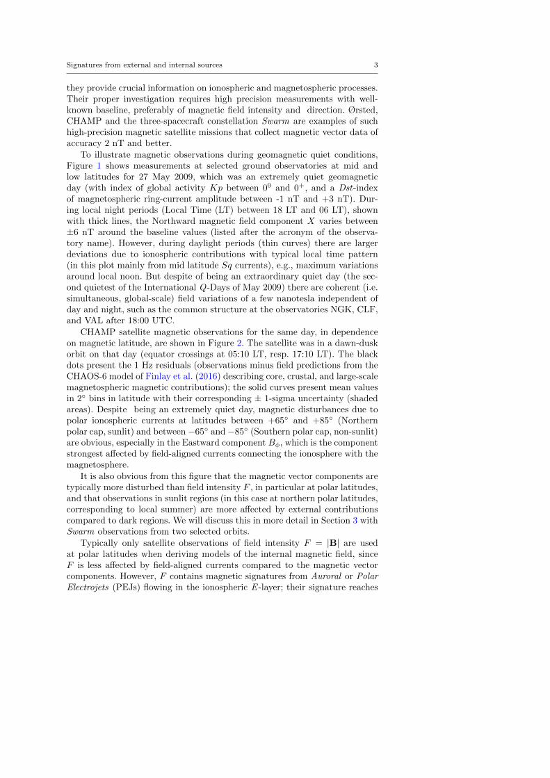
Signatures from external and internal sources 3

they provide crucial information on ionospheric and magnetospheric processes.Their proper investigation requires high precision measurements with well-known baseline, preferably of magnetic field intensity and direction. Ørsted,CHAMP and the three-spacecraft constellation Swarm are examples of suchhigh-precision magnetic satellite missions that collect magnetic vector data ofaccuracy 2 nT and better.

To illustrate magnetic observations during geomagnetic quiet conditions,Figure 1 shows measurements at selected ground observatories at mid andlow latitudes for 27 May 2009, which was an extremely quiet geomagneticday (with index of global activity Kp between 00 and 0+, and a Dst-indexof magnetospheric ring-current amplitude between -1 nT and +3 nT). Dur-ing local night periods (Local Time (LT) between 18 LT and 06 LT), shownwith thick lines, the Northward magnetic field component X varies between±6 nT around the baseline values (listed after the acronym of the observa-tory name). However, during daylight periods (thin curves) there are largerdeviations due to ionospheric contributions with typical local time pattern(in this plot mainly from mid latitude Sq currents), e.g., maximum variationsaround local noon. But despite of being an extraordinary quiet day (the sec-ond quietest of the International Q-Days of May 2009) there are coherent (i.e.simultaneous, global-scale) field variations of a few nanotesla independent ofday and night, such as the common structure at the observatories NGK, CLF,and VAL after 18:00 UTC.

CHAMP satellite magnetic observations for the same day, in dependenceon magnetic latitude, are shown in Figure 2. The satellite was in a dawn-duskorbit on that day (equator crossings at 05:10 LT, resp. 17:10 LT). The blackdots present the 1 Hz residuals (observations minus field predictions from theCHAOS-6 model of Finlay et al. (2016) describing core, crustal, and large-scalemagnetospheric magnetic contributions); the solid curves present mean valuesin 2◦ bins in latitude with their corresponding ± 1-sigma uncertainty (shadedareas). Despite being an extremely quiet day, magnetic disturbances due topolar ionospheric currents at latitudes between +65◦ and +85◦ (Northernpolar cap, sunlit) and between−65◦ and−85◦ (Southern polar cap, non-sunlit)are obvious, especially in the Eastward component Bφ, which is the componentstrongest affected by field-aligned currents connecting the ionosphere with themagnetosphere.

It is also obvious from this figure that the magnetic vector components aretypically more disturbed than field intensity F , in particular at polar latitudes,and that observations in sunlit regions (in this case at northern polar latitudes,corresponding to local summer) are more affected by external contributionscompared to dark regions. We will discuss this in more detail in Section 3 withSwarm observations from two selected orbits.

Typically only satellite observations of field intensity F = |B| are usedat polar latitudes when deriving models of the internal magnetic field, sinceF is less affected by field-aligned currents compared to the magnetic vectorcomponents. However, F contains magnetic signatures from Auroral or PolarElectrojets (PEJs) flowing in the ionospheric E -layer; their signature reaches

4 Olsen and Stolle

0 3 6 9 12 15 18 21 24

UT hours of May 27, 2009

-20

-15

-10

-5

0

5

10

15

[nT

]

CLF X - 21125 nT

NGK X - 18855 nT

VAL X - 19275 nT

HON X - 27115 nTHER X - 9650 nT

Fig. 1 Northward magnetic field component on 27 May 2009 as measured by the geo-magnetic observatories Niemegk/Germany (NGK), Chambon-la-Foret/France (CLF), Va-lencia/Ireland (VAL), Hermanus/South Africa (HER) and Honolulu/USA (HON). The ab-scissa shows time in UTC. Local night periods (Local time between 18 and 06) are shownwith thick lines; day periods with enhanced ionospheric contributions shown with thin lines.

amplitudes of 30 nT and more even during quiet periods and in dark regions.The signatures in F follow closely those in Br at high latitudes, since the fieldlines of the ambient magnetic field are almost vertical.

At nightside mid and low latitudes, where magnetic disturbances due toionospheric currents are expected to be weak, all three vector components(Br, Bθ, Bφ) are typically considered, whereas no data (neither F ) are used formagnetic field modelling at sunlit high-latitudes. The data that are typicallydiscarded for modelling the core and crustal field (since either from sunlitregions or vector components from polar latitudes) are indicated by shadedgrey in Figure 2.

Present geomagnetic field models describe the magnetic field observationswithin 2 nT on average (as an example: for the Swarm-derived model of Olsenet al. (2016) the non-polar root-mean-squared difference between the obser-vations used to derive the model and the model predictions varies between1.9 nT in Br and 3.0 nT in Bθ). Unmodeled ionospheric and magnetosphericfield contributions are arguably the main contribution to this rms-misfit of afew nanotesla (which exceeds measurement accuracy by almost one order ofmagnitude), and a better description of the time-space structure of these con-tributions (in particular for the extremely quiet conditions that are considered

Signatures from external and internal sources 5

Fig. 2 CHAMP satellite magnetic field residuals for 27 May 2009 (after removal of core,crustal and magnetospheric values as given by the CHAOS-6 model of Finlay et al. (2016))for the field intensity F and the vector components (Br, Bθ, Bφ), in dependence on QDlatitude (Richmond 1995). Data underlaid with grey are typically not used in geomagneticfield modelling.

in geomagnetic field modelling) will help to further improve models of the coreand crustal field.

In following we give a short overview of ionospheric and magnetosphericcurrent systems (section 2) followed by a discussion of their magnetic signatureas seen in Swarm satellite constellation observations, with focus on spatialgradient observations (section 3). As an example for a weak but systematicmagnetic signature that should be considered in geomagnetic field in orderto further improve the models, we discuss in section 4 the magnetic effect ofauroral field-aligned currents at mid and low latitudes.

2 Electric currents in the ionosphere and magnetosphere duringgeomagnetic quiet conditions

Extracting signals from electric currents during geomagnetically quiet condi-tions requires working with differences (residuals) between the magnetic obser-vations and model values from high-resolution empirical magnetic field models,in order to remove the typically much stronger contributions from the core,crust and (for ionospheric studies) the magnetosphere. Multipoint observa-tions from satellite constellation missions like Swarm enables an improved

6 Olsen and Stolle

characterisation of the spatial and temporal structures of weak ionosphericprocesses: when using the difference of magnetic field measurements taken byclose-by flying satellites. In that case the large-scale signals from the core andthe magnetosphere will cancel out. The differences preserve, however, mag-netic signatures at smaller scales (down to the separation of the spacecraft),thus allowing for investigating the time-space structure of electric currents inthe ionosphere in a novel way. But also for these studies it is crucial to ac-count for crustal field signatures since they occur at similar length scales andamplitudes as the ionospheric currents in consideration.

Ionospheric and magnetospheric contributions are typically rather differentin polar, mid latitude, and equatorial regions. In addition, ionospheric signalsare different on the day- and night side, mainly because ionospheric conduc-tivity is greatly affected by solar irradiation, dropping essentially to zero inthe ionospheric E -layer during night.

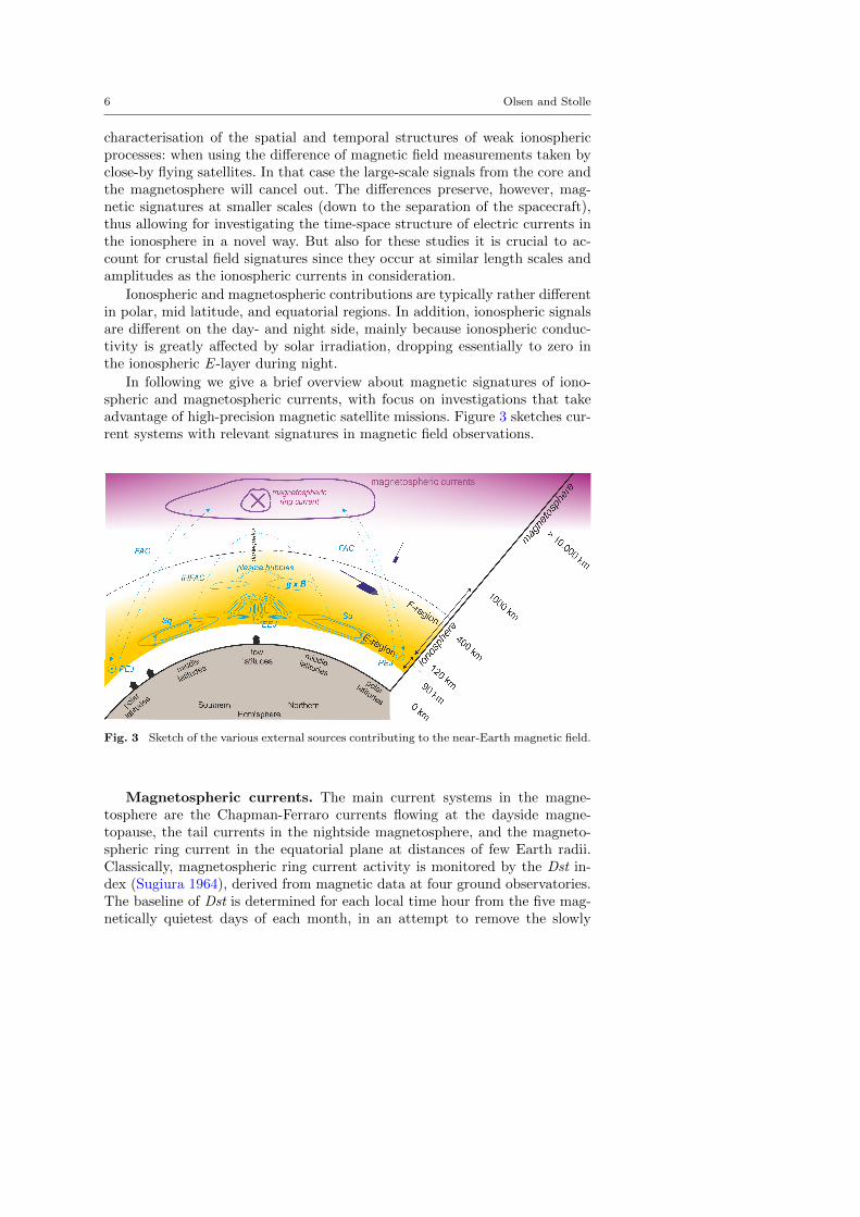
In following we give a brief overview about magnetic signatures of iono-spheric and magnetospheric currents, with focus on investigations that takeadvantage of high-precision magnetic satellite missions. Figure 3 sketches cur-rent systems with relevant signatures in magnetic field observations.

Fig. 3 Sketch of the various external sources contributing to the near-Earth magnetic field.

Magnetospheric currents. The main current systems in the magne-tosphere are the Chapman-Ferraro currents flowing at the dayside magne-topause, the tail currents in the nightside magnetosphere, and the magneto-spheric ring current in the equatorial plane at distances of few Earth radii.Classically, magnetospheric ring current activity is monitored by the Dst in-dex (Sugiura 1964), derived from magnetic data at four ground observatories.The baseline of Dst is determined for each local time hour from the five mag-netically quietest days of each month, in an attempt to remove the slowly

Signatures from external and internal sources 7

changing core field (secular variation). However, this procedure also removessome quiet-time signals of the ring current. Other indices monitoring the mag-netospheric ring-current have therefore been suggested, derived from groundobservatories and/or satellite observations (see Kauristie et al., this issue). Oneof them is the RC-index (Olsen et al. 2014), which is determined using datafrom up to 21 ground observatories after subtraction of the core field as givenby a geomagnetic model. RC is levelled to the average of quiet time data overseveral years (as opposed to the annual levelling of Dst). The variations of RCclearly show an evolution of the ring current signatures of several nanoteslawithin weeks and months, similar to what is seen in satellite-derived indicesof ring-current activity.

Since the baseline of ground observatory is undetermined (due to the staticbut unknown contribution from the regional crustal field in the vicinity of theobservatory), the absolute value of the ring current signature during quiettimes (that is the strength of the ring-current for zero value of RC or Dst)can only be determined with high-precision geomagnetic LEO satellites. Sug-iura et al. (1971); Sugiura (1972) and Sugiura and Poros (1973) used magneticintensity measurements taken by the OGO satellite series to derive models ofthe magnetospheric ring current. Langel and Estes (1985a,b) extended theseinvestigations and determined the ring current quiet time level (for Dst = 0) to−20 nT based on data from the Magsat satellite. Using Ørsted and CHAMPobservations, Maus and Luhr (2005) and Luhr and Maus (2010) further sepa-rated the large scale magnetospheric signatures into one part originating fromthe ring current, and another part originating from tail and magnetopausecurrents. Tail and magnetopause currents are found to be independent on so-lar flux variations, but the ring current contribution seems to vanish for verylow solar flux. Correspondingly, Sabaka et al. (2015) revealed a quiet time ringcurrent contribution of less than −5 nT for the years 2009 and 2010 (solar fluxas low as F10.7 = 70× 10−22Wm−2Hz−1) while nearly −40 nT were found forthe solar maximum years 2002 and 2003.

The dependence of the ring current magnetic signal on local time has beeninvestigated for moderate and active times using satellite and ground magneticobservations (e.g., Le et al. 2011; Newell and Gjerloev 2012). These authorsfound that the ring-current magnetic signature is several nanotesla stronger(more negative) in the evening (around 18 LT) compared to morning (around06 LT). However, in-situ ring current observations derived from magnetometerobservations of the Cluster mission revealed stronger currents on the dawnside compared to the dusk side (Zhang et al. 2011), reflecting a ring currentlocal-time asymmetry opposite to that found in groundbased or LEO satellitemagnetometer data. The reason for this difference is unknown but could bedue to the fact that the Cluster satellites measure an in-situ current densitywhile LEO satellites observe the integrated effect of all currents comprisingthe magnetospheric ring current and auroral FACs. The near Earth effects oflarge scale magnetospheric currents is discussed in more detail by Luhr et al.(this issue).

8 Olsen and Stolle

A small, but significant difference in the amplitude of ring current magneticsignatures between LEO satellites and ground has been noticed in earlier years(e.g., Langel and Estes 1985b; Olsen 2002; Maus and Luhr 2005). Recently,Le et al. (2011) compared C/NOFS satellite observations with the Dst-indexfor selected geomagnetic storms and found that the satellite observations haveonly about 80% amplitude of the signatures at ground. Whether this differenceis due to different processing of ground and satellite data, or whether it reflectsan additional current flowing in the ionosphere (i.e. between ground and LEOsatellite altitudes) as suggested by Fukushima (1989), is still unclear.

Ionospheric currents. The polar ionosphere is coupled to the magneto-sphere via Field-Aligned Currents (FACs). Ionospheric E -layer currents, suchas the polar electrojets, and FACs are always present, although of varying in-tensity depending on activity. They are caused by magnetospheric convection,mapping an electric field down to the ionosphere.

Minimum contributions from ionospheric and magnetospheric currents inpolar regions are expected for dark conditions and low geomagnetic activity.Magnetic signals of few tens of nanotesla are attributed to the Polar Elec-trojets (PEJs) as is also seen in Figure 2, and later in Figures 4 to 6 of thisarticle. Ritter and Luhr (2006) used CHAMP satellite magnetic observationsto characterize the variability of external contributions at auroral latitudes forgeomagnetic quiet and dark conditions. They found the strength of the PEJsto be neither correlated with the strength of FACs nor with solar wind pa-rameters. However, there is a clear correlation for more active or sunlit times.Further investigations on possible statistical or physical relations to magne-tospheric or solar wind proxies are needed to better characterize very quietconditions at auroral latitudes – and thereby helping scientists deriving coreand crustal field models to select data that are least contaminated by externalsources.

Swarm constellation magnetic data enable to estimate the spatial and tem-poral scales of auroral FACs. Luhr et al. (2015) found that small scale currents(with horizontal scales of < 10 km) persist for only 10 s and are locally con-fined, while currents of larger (> 150 km) scales persist up to 60 s. Thisanalysis is based on data from the beginning of the Swarm mission when thethree satellites flew in a “string-of-pearls-configuration”, with only marginallongitudinal separation. FACs are assumed in that study to be organized asinfinite extended current sheets, an assumption that, however, might not bevalid in particular for small-scale FACs.

At mid latitudes, the prominent ionospheric currents are the Sq (solarquiet) currents of the ionospheric dynamo. This current system consist of twovortices with foci at about ±30◦ magnetic latitude centred around local noonand currents flowing anticlockwise in the Northern hemisphere, and clockwisein the Southern hemisphere when looking from above the ionosphere. Polarorbiting satellites measure along North-South oriented profiles, and are there-fore well suited to resolve their global extension and variability. Pedatella et al.(2011); Sabaka et al. (2015) and Chulliat et al. (2016) derived climatologicalmodels of the mid latitude Sq. However, the Sq currents exhibit significant

Signatures from external and internal sources 9

day-to-day variations (e.g., Yamazaki et al. 2011), that clearly need to beconsidered for single event analyses.

High-precision magnetic observations from LEO satellites can also resolvethe weak interhemispheric field-aligned currents (IHFACs) that flow due todifferences in the electrostatic potential between the two Sq vortices. Althoughtheir existence has been predicted in the 1960s by van Sabben (1966), it tookmore than 30 years to detect them in satellite observations (Olsen 1997). Luhret al. (2015) studied their local time and longitudinal variations using Swarmsatellite constellation data and found enhanced southward directed IHFACsduring noon at longitudes of the South Atlantic Anomaly, suggesting that theweak core field in that region enhances the Sq current strength in the Southernhemisphere.

Magnetic signatures from Medium Scale Travelling Ionospheric Distur-bances (MSTIDs) are detectable during dark conditions, when the effects fromSq is reduced, in the components perpendicular to the main magnetic field.MSTIDs are regionally confined nighttime dynamic plasma density irregular-ities in the ionospheric E - and F -layers associated with electric field fluctu-ations that map to both conjugate hemispheres and thus produce significantIHFACs (Shiokawa et al. 2003). They have first been found by Saito et al.(1995) in electric measurements taken by the DE-2 satellite, and by Parket al. (2009) in magnetic field observations taken by the CHAMP satellite.Using data from the Swarm constellation, Park et al. (2015) confirmed thattheir spatial structure is similar to those of the associated plasma densityfluctuations.

At dayside low latitudes the Equatorial Electrojet (EEJ) is the most promi-nent feature in magnetic observations at satellite altitudes. This current flowspredominantly eastward along the magnetic equator within a band of ±2◦

latitude. Although the EEJ is known since many years from magnetic ob-servations from ground (e.g., Onwumechili 1967; Forbes 1981), only satelliteobservations from Ørsted and CHAMP provided a global picture of the EEJand its LT dependence (Ivers et al. 2003; Luhr et al. 2004). Alken and Maus(2007) derived a climatological model of the EEJ sheet current density basedon Ørsted, SAC-C and CHAMP observations, describing its variability withlongitude, season, local time, and solar flux. Comparing EEJ estimates basedon CHAMP data with ground based magnetic data, Manoj et al. (2006) re-vealed a longitudinal correlation length of the day-to-day variability of theEEJ of ±15◦, which has been attributed to similar characteristic lengths ofthe ionospheric conductivity. Based on the side-by-side flying satellite SwarmAlpha and Charlie, Alken et al. (2015) investigated the gradient of the equa-torial electric field. They revealed that also the longitudinal gradient of theelectric field, similar to the electric field and the EEJ itself, exhibits significantlongitudinal variability which is attributed to coupling to upward propagatingatmospheric waves.

On the nightside, when the E-region conductivity is depleted, the low lat-itudes are affected by F -region diamagnetic and gravity driven currents inparticular during the hours after sunset. Based on analyses from CHAMP and

10 Olsen and Stolle

Swarm satellite observations, Alken (2016) found a correlation above 0.7 be-tween in situ electron density and total magnetic field above the ionisationmaximum (e.g., above 400 km altitude) which supports the significance of dia-magnetic currents at these altitudes after sunset. The total field perturbationshave been found to be up to few nanotesla before midnight and are strongestduring equinoxes.

Diamagnetic and field-aligned currents associated with post-sunset plasmairregularities in the nightside ionosphere are yet another source of magneticdisturbances. They occur regularly after sunset at the equator at the bottomof the F -region. The structure rises, expands upward and extends poleward.The lifetime of these structures is between several minutes to hours (see, e.g.,Woodman 2009, for a review). The magnetic signatures of these plasma irreg-ularities have first been detected in LEO satellite data by Luhr et al. (2002),and their dependence on season, longitude and solar flux was determined byStolle et al. (2006). Motivated by these observations, Yokoyama and Stolle(this issue) discuss physical modelling of post-sunset plasma irregularities toexplain the observed magnetic signatures.

3 On the spatial gradients of magnetic variations caused byionospheric and magnetospheric currents

High precision geomagnetic satellite missions in low Earth orbits are an im-portant tool for studying ionospheric and magnetospheric current systems.Recently, also “differential data”, either along satellite tracks (first time differ-ences) from single satellites, or differences of measurements taken by close-bysatellites, have provided further insight in small-scale structures of the up-per atmosphere and magnetosphere, in particular those which are also presentduring quiet conditions.

To demonstrate the variability of magnetic field variations caused by elec-tric currents in near Earth space, we will first present two exemplary events,representative for dayside and nightside conditions, followed by a statisticalanalysis of magnetic field variations and their variability for different localtimes. As pointed out by Fukushima (1994), “... complicated phenomena [...]must be discussed both statistically and for individual examples; these twodifferent approaches are really complementary and not to be confronted eachother”.

3.1 Two example orbits from the day-, respectively night-side

Magnetic field intensity residuals along the dayside part of one orbit of thetwo Swarm satellites Alpha and Charlie are presented in Figure 4. The se-lected orbit, with an equatorial local time crossing at 12:12 LT, is from 2 May2014, which was a geomagnetic quiet day (Kp < 1+ and Dst > −13 nT);the ground track of this orbit is shown in the lower right part of the figure.

Signatures from external and internal sources 11

The left column (panels 4 a,d,g) shows observations from Swarm Alpha; themiddle column (panels 4b,e,f) presents an estimate of the East-West gradientas measured by Swarm Charlie minus Swarm Alpha, divided by the distancebetween the two spacecraft; the right column (panels 4c,f,i) shows an estimateof the North-South gradient, obtained from 15-seconds alongtrack differencesof Swarm Alpha divided by d = 141 km (which is the distance of two satellitemeasurements taken 15 seconds apart). For each of the three columns, theblue curves present the difference ∆F = Fobs − Fmod between observed mag-netic intensity Fobs and model values Fmod as given by the CHAOS-6 modelof Finlay et al. (2016), whereas the red curves show model predictions.

Figure panels 4a,b,c present (blue curves) measurements minus core fieldmodel values, and (red curves) model predictions of the lithospheric field. Themiddle row of the figure (panels 4d,e,f) shows (blue curves) measurements mi-nus model values of core and crustal field, and (red curves) model predictionsof the magnetospheric field. Finally, panels 4g,h,i present (blue curves) mea-surements minus model values of the core, crustal and magnetospheric field,and (red curve) predictions of the ionospheric field as given by the CM5 modelof Sabaka et al. (2015). The yellow curve in panel 4g shows observations fromsatellite Swarm Charlie.

After subtracting the CHAOS-6 core, crustal and magnetospheric modelpredictions from the observations (blue curve of Fig. 4g) the signature of theEquatorial Electrojet is clearly visible at the magnetic equator (0◦ QD lat-itude) as a depression of magnetic field intensity F . The minima at about±30◦ latitude probably reflect signatures of the mid latitude Sq current. Us-ing ground magnetic observations, Yamazaki et al. (2011) identified the focusof Sq at about 30◦ magnetic latitude, where the Z-component shows a localextreme and the North component minimizes. Stolle et al. (2016) present anSq event as seen in Swarm satellite observations of December 2013; in this ex-ample the extreme in F collocates approximately with the extreme in Z andthe North component minimizes at approximately the same latitude whereZ maximizes. The observations in Figure 4g show similarity to these results.However, other current sources such as interhemispheric field-aligned currents,F region currents or possible effects from ground conductivity have not beenconsidered here. Substantial magnetic variations occur in the auroral regions,especially in the sunlit northern hemisphere where ionospheric conductivity ishigher compared to the dark southern hemisphere, resulting in stronger PolarElectrojets.

The East-West gradient of ∆F , shown in Figure panel 4h, reveals maximaat the equatorial edges of the Sq current system, of up to 7 pT/km in thisexample. The gradient of the EEJ is smaller in magnitude than that of Sq,indicating rather weak East-West (i.e. local time) variation of the EEJ for thenoon conditions presented here.

Panel 4i provides the South-North gradient, which for Sq is of similar am-plitude compared to the East-West gradient. However, the signal of the EEJis much larger in that gradient component, reflecting its narrow extension inlatitude (thus resulting in a large South-North gradient) but extended struc-

12 Olsen and Stolle

ture in longitude (i.e. small East-West gradient). The largest gradients occur,however, in the auroral regions and are caused by the PEJs.

We now shortly come back to the gradients of the mid-latitude signaturesin Figures 4h,i to discuss possible contributions from the E -region Sq systemor F -region currents. Alken (2016) published a statistical study of Swarm mag-netic observations including alongtrack differences of the North component atmid- and low latitudes. Beside strong signatures around the dip equator hefound a maximum/minimum of the alongtrack differences at about 15◦, resp.−20◦, magnetic latitude during pre-noon hours, and suggested that those re-sult from F -region diamagnetic and gravity driven currents being collocatedwith the crests of the Equatorial Ionisation Anomaly. Figure 4i does not indi-cate such a behaviour for this example, but rather reveals a maximum at 40◦

magnetic latitude. Figure 4h shows the East-West gradients in scalar intensityF with maximum at −10◦ magnetic latitude. However, when comparing withFigures 4k,i showing plasma densities, these extrema do not collocate withextrema in plasma density or plasma density gradients. We therefore concludethat gravity driven and diamagnetic F -region currents do not significantly af-fect Swarm observations during daytime when E -region currents are strong.

The gradients of the magnetospheric field as provided by the CHAOS-6model, shown in Figure panels 4e,f by the blue line, are rather different in theEast-West and South-North gradients: While there is hardly any East-Westgradient (i.e. CHOAS-6 model for satellite tracks Swarm Alpha and Char-lie shows an almost identical magnetospheric (field), the alongtrack gradienthas maxima at low latitudes, with changing sign between the hemispheres, asexpected for the magnetic signature of the magnetospheric ring current. A dif-ference in electron density of 0.2× 106 cm−3 is expected to create a magneticsignal of about 0.2 nT which is at the limit of detectability by high precisionsatellites (Stolle et al. 2006). In Figure 4 this would correspond to 1.4 pT/km,anti-correlated with the plasma density gradient.

Figure panels 4g,h,i show (red curves) predictions of the ionospheric fieldas given by the CM5 model of Sabaka et al. (2015). The model describes theEEJ signatures in general rather well, and roughly reflects the amplitude of Sqfor this example. This also holds for the South-North gradient; the ringing atnorthern mid latitudes is probably due to constraining the spherical harmonicexpansion of the CM5 ionospheric field. The East-West gradients at mid andlow latitudes are however not well described by CM5 in this example; they dofor instance not show any of the observed features connected to the equator-ward edges of Sq. Alongtrack gradient information from the CHAMP satellitecontributed to CM5, and taking advantage of East-West gradient data fromSwarm will likely improve the model further.

The red curves in the top row represent the magnitude (Figure 4a) andthe gradients (Figures 4b,c) of the lithospheric field as given by the CHAOS-6model. East-West and South-North gradients of the lithospheric field are ofsimilar magnitude as the ionospheric signatures during day time; demonstrat-

Signatures from external and internal sources 13

F [nT] δFEW [pT/km] δFNS [pT/km]

∆F

-90° -60° -30° 0° 30° 60° 90°

-40

-20

0

20

a

-90° -60° -30° 0° 30° 60° 90°-30

-20

-10

0

10

20

30

b

-90° -60° -30° 0° 30° 60° 90°-30

-20

-10

0

10

20

30

c

∆F

-90° -60° -30° 0° 30° 60° 90°

-40

-20

0

20

d

-90° -60° -30° 0° 30° 60° 90°-30

-20

-10

0

10

20

30

e

-90° -60° -30° 0° 30° 60° 90°-30

-20

-10

0

10

20

30

f

∆F

-90° -60° -30° 0° 30° 60° 90°

-40

-20

0

20

g

-90° -60° -30° 0° 30° 60° 90°-30

-20

-10

0

10

20

30

h

-90° -60° -30° 0° 30° 60° 90°-30

-20

-10

0

10

20

30

i

QD-latitude QD-latitude QD-latitude

Ne×

106

[cm

−3]

-90° -60° -30° 0° 30° 60° 90°0

1

2

k

-90° -60° -30° 0° 30° 60° 90°-2

-1

0

1

l-180 -120 -60 0 60 120 180

-90

-60

-30

0

30

60

90

3

Fig. 4 Magnetic field intensity residuals for the day-time part of Swarm orbit number 2464of 2 May 2014 vs. QD latitude. Equator crossing at 18:43:04 UT, corresponding to 12:12Local Time.(a,b,c): The blue curve shows the difference ∆F = Fobs−Fcore between observed magneticintensity Fobs and the core field part Fcore as given by the CHAOS-6 model. The red curveshows the crustal field model predictions. (d,e,f): The blue curve presents the differencebetween the two curves of panels (a,b,c), i.e., the observed values minus model values forcore and crust. The red curve shows the modelled contributions of magnetospheric currents.(g,h,i): The magnetic field intensity after removal of core, crustal and magnetospheric modelvalues (shown by the red curves in panels d,e,f) is shown in blue. The red curves presentsionospheric current contributions as given by the CM5 model. Left panel shows values forSwarm Alpha; middle panel presents East-West gradients based on data from Swarm Charlieminus Swarm Alpha; right panel shows alongtrack gradients of Swarm Alpha.Bottom: Electron density Ne as measured by Swarm Alpha (left), and difference SwarmCharlie minus Swarm Alpha (middle). Ground track of the chosen satellite orbit, withhighlighted dayside part, is shown in the bottom right panel. The yellow curves in panels kand l shows observations from satellite Swarm Charlie.

14 Olsen and Stolle

ing the importance of accounting for lithospheric contributions when analysingionospheric currents.

Electron density, shown in the bottom row of Figure 4, is highest at equa-torial latitudes, indicating the strength of the equatorial ionisation anomaly atsatellite altitude. Its East-West gradient (shown here as the difference of theobservations taken by Swarm Charlie and Alpha) is rather small for this orbitand thus has only insignificant impact on the magnetic field. The magneticfield variations are therefore dominated by E -region and magnetospheric cur-rents; diamagnetic effects due to electron density differences play only a veryminor role.

F -region currents are much more important in the orbit presented in Fig-ure 5. It shows magnetic field intensity residuals along a night side orbit on25 October 2014 (local time of 20:30 LT). Although this was a day of slightlyhigher geomagnetic activity (Kp < 30 and Dst ≥ −30 nT) it can still beconsidered as a geomagnetically quiet period. E -region conductivity is greatlyreduced during night at low and mid latitudes, and thus no signatures fromnon-polar E -region currents are expected in the magnetic residuals shown inFigure 5g; they are indeed weak at these latitudes. Despite this, both SwarmAlpha and Swarm Charlie observe, at both sides of the magnetic equator,field depletions of few nanotesla which are interrupted by small-scale positivespikes. These spikes occur in the southern hemisphere for Swarm Charlie andin the northern hemisphere for Swarm Alpha. These variations are caused bydiamagnetic F -region currents that arise due to steep plasma density gradientsat post sunset local times. The bottom row of Figure 5 shows a well developedequatorial ionisation anomaly, characterized by a double hump to the north,respectively south, of the magnetic equator. Ionisation anomalies after sun-set are frequently affected by equatorial plasma density irregularities at about±10◦ magnetic latitudes, often called “plasma bubbles”, for instance at +10◦

magnetic latitude for Swarm Alpha and at −10◦ magnetic latitude for SwarmCharlie in Figure 5. Although the amplitudes of their magnetic signatures areonly few nanotesla, the obvious spatial anti-correlation between electron den-sity and magnetic signature clearly identifies the origin of these signature inF .

The electron density measured by Swarm Alpha and Charlie shows spatialdifferences. Its increase from West to East (i.e. towards later local times) at thetrough of the ionisation anomaly at the magnetic equator reflects the decreaseof the magnetic anomaly, as expected for this local time (Liu et al. 2007).Indeed the magnetic signature between the two satellites decreases in responseto the reduced diamagnetic effect. For the presented orbit, the magnetic fieldgradients due to post sunset electrodynamics are of similar magnitude as thosein auroral regions. They are smaller in the magnetic South-North gradientcompared to the East-West gradient since post-sunset plasma irregularitiesare likely aligned with the ambient magnetic field (e.g., Immel et al. 2003).Diamagnetic currents due to variations of the ionisation anomaly are discussedby Alken et al. (this issue).

Signatures from external and internal sources 15

F [nT] δFEW [pT/km] δFNS [pT/km]

∆F

-90° -60° -30° 0° 30° 60° 90°

-40

-20

0

20

a

-90° -60° -30° 0° 30° 60° 90°-30

-20

-10

0

10

20

30

b

-90° -60° -30° 0° 30° 60° 90°-30

-20

-10

0

10

20

30

c

∆F

-90° -60° -30° 0° 30° 60° 90°

-40

-20

0

20

d

-90° -60° -30° 0° 30° 60° 90°-30

-20

-10

0

10

20

30

e

-90° -60° -30° 0° 30° 60° 90°-30

-20

-10

0

10

20

30

f

∆F

-90° -60° -30° 0° 30° 60° 90°

-40

-20

0

20

g

-90° -60° -30° 0° 30° 60° 90°-30

-20

-10

0

10

20

30

h

-90° -60° -30° 0° 30° 60° 90°-30

-20

-10

0

10

20

30

i

QD-latitude QD-latitude QD-latitude

Ne×

106

[cm

−3]

-90° -60° -30° 0° 30° 60° 90°0

1

2

k

-90° -60° -30° 0° 30° 60° 90°-2

-1

0

1

l-180 -120 -60 0 60 120 180

-90

-60

-30

0

30

60

90

4

Fig. 5 Similar to Figure 4 but for the nightside part of Swarm Alpha orbit number 5151on 25 October 2014. Equator crossing at 01:16:09 UT, corresponding to 20:30 Local Time.

3.2 Statistical analysis

A more comprehensive picture of the magnetic signatures of ionospheric cur-rents at satellite altitude, including their horizontal gradients, is provided by astatistical analysis of two years (December 2013 to December 2015) of Swarmresiduals (observations minus core, crustal and magnetospheric contributionsas given by CHAOS-6, similar to what was shown in Figures 4g,h,i and 5g,h,ifor single tracks) for quiet conditions (Kp ≤ 2o, |dDst/dt| < 2 nT/hr). Thetop row of Figure 6 presents how the mean magnetic field residuals, for vari-ous LT windows, depend on QD-latitude; the black thick line shows data for“dark” conditions (sun at least 10◦ below horizon, a selection criteria thatis often used in geomagnetic field modelling). The bottom row presents thecorresponding standard deviation σ.

16 Olsen and Stolle

The most prominent features in all panels are the signatures of the PolarElectrojets at ±70◦ to ±80◦ magnetic latitude. Mean amplitudes reach 30 nTeven during the quiet conditions considered here, but with standard deviationσ of similar amplitude. This indicates a considerable variability, reducing thesignificance of using average values to describe the PEJs. Similar to what isseen in the single orbit example of the previous section, the prominent currentin the dayside equatorial regions is the Equatorial Electrojet. It develops in themorning, has its maximum around local noon, and decreases in the afternoon.Both the EEJ and the Sq current signatures are largest around noon (10 LT– 12 LT) and persist with significant amplitudes during post-noon (14 LT –18 LT), corresponding to remaining E -region conductivities during those localtimes. During night time, the mean values are, as expected, close to zero at

-90° -60° -30° 0° 30° 60° 90°-40

-30

-20

-10

0

10

20

∆F

[nT

]

Field F

a

-90° -60° -30° 0° 30° 60° 90°-20

-15

-10

-5

0

5

10

15

20

∆δF

[pT

/km

]

East-West Gradient δF

c

-90° -60° -30° 0° 30° 60° 90°-20

-15

-10

-5

0

5

10

15

20

∆δF

[pT

/km

]

Alongtrack Gradient δF

e

-90° -60° -30° 0° 30° 60° 90°

QD-latitude

10-1

100

101

σ∆

F [n

T]

b

02 MLT - 06 MLT06 MLT - 10 MLT10 MLT - 14 MLT14 MLT - 18 MLT18 MLT - 22 MLT22 MLT - 02 MLTdark

-90° -60° -30° 0° 30° 60° 90°

QD-latitude

100

101

102

σ∆δF [p

T/k

m]

d

-90° -60° -30° 0° 30° 60° 90°

QD-latitude

100

101

102

σ∆δF [p

T/k

m]

f

Fig. 6 Top: Mean value of field intensity residuals during quiet days, after removal of core,crustal and magnetospheric contributions, in dependence on QD-latitude and for variousLocal Time windows. Bottom: Corresponding standard deviation.Left: Field intensity F ; Middle: East-West gradient (based on difference Swarm Charlieminus Swarm Alpha); Right: Alongtrack gradient (based on first differences of 15 secondsdata of Swarm Alpha).

non-polar latitudes, while at high latitudes significant variations occur at alllocal times as discussed in Section 2.

The non-polar ∆F is slightly positive in the morning (02 LT – 06 LT and06 LT – 10 LT) and negative in the evening sector (18 LT – 22 LT), indicatinga large-scale source that varies with local time but is not restricted to thedayside. Newell and Gjerloev (2012) found a local time dependence of the sig-nature of the magnetospheric ring current, being strongest in the evening and

Signatures from external and internal sources 17

weakest in the morning. A similar behaviour is seen in Figure 6a. Since theseresults are derived from differences between observations and model valuesincluding core, crustal and a magnetospheric contribution that has no localtime dependence, the clear difference between dusk and dawn in the statisticalanalysis indicates an asymmetric magnetospheric ring current, extending thefindings of Newell and Gjerloev (2012) (which were obtained for geomagneticactive conditions) to the quiet times considered here.

Standard deviations (Figure 6b) show enhanced variability of magneticsignatures near the equator for all local times, including night. This reflects theexistence of remaining F -region currents, such as dynamo, gravity or pressuregradient driven currents that affect the total field also after sunset. Thesecurrents have longitudinal, seasonal and day-to-day variations for which wedid not distinguish for in this graph, also contributing to observed standarddeviations. The variability is smallest at post-midnight (02 LT – 06 LT) whenF -region ionisation is lowest and the ionisation anomalies generally vanish(e.g., Stolle et al. 2011; Liu et al. 2007).

Figure 6c shows mean values of the East-West gradient of scalar intensityresiduals. Significant gradients are expected in polar regions where the iono-sphere is temporally and spatially highly dynamic due to intense magnetosphere-ionosphere coupling. At equatorial latitudes, the effect of the EEJ results in anincrease of about 1 pT/km towards East in the morning and a decrease of sim-ilar amplitude in the afternoon, which is reasonable since the EEJ grows aftersunset and decreases after noon. The East-West gradient is reduced aroundnoon when the EEJ maximizes. In contrast, the Sq currents seem to havelargest East-West gradients around noon.

Night side residuals show weak East-West gradients. Similar to Figure 6a,lowest gradients occur around midnight, with preferred offsets after sunset(18 LT – 22 LT) and before sunrise (02 LT – 06 LT). Apparently, also thegradient of the ring current signatures shows a local time asymmetry similarto that of the ring current itself.

Figure 6d presents the corresponding standard deviations. Largest vari-ability is found in polar and auroral regions. Variability of the mid latitudesSq currents follows that of the gradient itself, with largest values around localnoon. At equatorial latitudes the climatology and day-to-day variability of theEEJ is responsible for the local maximum of the standard deviation. Variabil-ity on the night side is much reduced although there are distinct peaks around±10◦−15◦ magnetic latitude. They correspond to the peaks of the post sunsetionisation anomaly that has significant negative gradients toward later localtimes. This local time variation is not seen in the average gradients (panel 6c);its variability (panel 6d) is however significant. The relation to ionisation isfurther confirmed by the absence of this double peak at pre-sunrise. In gen-eral the East-West gradient and its variability (Figure 6c,d) is larger at polarcompared to low and mid latitudes, for all local times.

The South-North (alongtrack) gradient for satellite Swarm Alpha is shownin Figure 6e. It is below 1 pT/km at mid latitudes, indicating weak ionosphericand magnetospheric contributions in the average alongtrack gradients. This is

18 Olsen and Stolle

different at low and auroral latitudes where the EEJ and the PEJ cause gradi-ents of up to 10 pT/km. The standard deviation of the South-North gradient(Figure 6f) has about the same magnitude, or is even larger, as the gradientitself (Figure 6f) for all latitudes and local times, indicating the large orbit-to-orbit variability of the alongtrack gradients. This variability is, however,lowest at middle latitudes during nighttime; the determined values of around0.1 pT/km reflect probably the accuracy of the magnetic measurements of theSwarm satellites.

The black thick curves in all panels are obtained using data from “dark”conditions that are typically chosen for modelling of the Earth’s internal mag-netic field. At mid and low latitudes the black line follows mainly the behaviourof data around midnight (22 – 02 LT) with tendency toward the post-sunsetstructures (18 – 22 LT) especially for the standard deviations. The curves forpre-sunrise (02 – 06 LT) are always less disturbed than the dark time curves.At polar latitudes, the selection for dark hours seems to improve the situationcompared to the selected local times, but the amplitudes in both field strengthand gradients are still significant, and further selection criteria or parametriza-tion will have to be defined to further reduce residuals. Saying this, a lot ofunexplained physics in the ionosphere/magnetosphere during very quiet timesstill needs to be understood.

4 Magnetic signature of Region-1/2 Field-Aligned Currents atnon-polar latitudes

As an example of a weak but persistent magnetic signature at all latitudeswe finally discuss the magnetic field caused by polar Field Aligned Currents(FACs).

Currents flowing along magnetic field lines of the ambient magnetic field,connecting the polar ionosphere and the distant magnetosphere, are more orless always present – even during geomagnetic quiet days. These Field AlignedCurrents are mainly organized in East-West oriented sheets, resulting in in-situsatellite magnetic field variations in the East-West component Bφ, and onlymarginal impact on the component B‖ in the ambient field direction (i.e. mag-netic field intensity F ). Satellite magnetic measurements of Bφ have thereforebeen used to investigate these current systems in the polar ionosphere. FACson the high latitude side of the auroral zone are referred to as Region-1 cur-rents, while those on the low latitude side are referred to as Region-2 currents,as sketched in the lower left panel of Figure 7. Maps of FACs in dependenceon e.g. season and the Interplanetary Magnetic Field (IMF) have been derivedby data from the satellites Dynamics Explorer-2 (e.g., Weimer 2001), Iridiumconstellation (e.g., Waters et al. 2001), Magsat and Ørsted (e.g., Christiansenet al. 2002) and CHAMP (e.g., He et al. 2012).

When flying through the auroral zones with their non-zero FACs, the mag-netic field B measured by LEO satellites can not be represented as a Laplacianpotential field, i.e. B 6= −∇V with V as the magnetic scalar potential, due to

Signatures from external and internal sources 19

6

Fig. 7 Top: Radial current density at top of the ionosphere in the Northern (left), respec-tively Southern (right) polar cap, as determined by Laundal et al. (2016) (their Fig. 3)for Northern winter conditions, in dependence on QD-latitude and MLT. The equatorwardboundary is at ±55◦ QD-latitude.Bottom: 3D current system connection horizontal ionospheric currents with the distantmagnetosphere through FACs. Left: Sketch of Region-1/2 currents. Right: Radial currentsat top of the ionosphere and their closure through Region-1/2 currents. One satellite orbitis sketched in yellow, with QD latitudes equatorwards of ±55◦ highlighted.

non-zero current density j, resulting in ∇×B = µ0j 6= 0. Outside the auroralzones, the current density at satellite altitude is close to zero (apart from possi-ble inter-hemispheric currents, which, however, are much weaker compared tothe auroral FACs, as discussed in section 2). Thus the magnetic field at middleand low latitudes (i.e. outside the auroral zone) is a Laplacian potential fieldand thus a representation B = −∇V is possible in those regions. However, aglobal representation of magnetic field variations, for instance using sphericalharmonics, is still not possible since this would require ∇×B = 0 in the wholesampling shell, which means at all latitudes, as explained in more detail e.g.in Olsen et al. (2010).

20 Olsen and Stolle

As mentioned above, Region-1/2 currents continue from the auroral iono-sphere along field lines of the Earth’s main field to the magnetosphere. Thecomplete 3D current system comprises horizontal currents (PEJs) in the auro-ral ionospheric E -layer, FACs (the Region-1/2 currents) and closing currentsin the distant magnetosphere. This 3D current system causes magnetic fieldvariations at all latitudes, also in the non-polar regions where∇×B = µ0j = 0.

To investigate this effect we constructed a 3D current system from theradial current density jr at the top of the polar ionospheric E -layer as de-termined by Laundal et al. (2016) for Northern winter conditions and IMFBz < −1 nT (see their Fig. 3). Their determined radial current density isshown in the top panel of Fig. 7. The complete 3D current system consists (i)of horizontal sheet currents JH in the ionosphere that are constructed from∇ · JH = −jr (taking advantage of the fact that the 3D current density j hasto be divergence-free), (ii) of a current density j‖ connecting the ionosphereand the magnetosphere along dipole field lines, and (iii) of closing currents inthe distant magnetosphere (at distance of 20 Earth radii).

We determined the magnetic signatures produced by this 3D current sys-tem using the poloidal-toroidal decomposition approach of Engels and Olsen(1998). Figure 8 shows the obtained magnetic field variations for a typical satel-lite altitude of 400 km. As expected, the largest amplitudes occur at aurorallatitudes where the magnetic horizontal components reaches 90 nT (170 nT)in Bθ in the Northern (Southern) hemisphere, and 140 nT (210 nT) in Bφ.Amplitudes are much smaller (< 17 nT) in the radial component Br, and evensmaller (< 6 nT) in field intensity F , as expected for magnetic fields mainlyproduced by FACs.

The magnetic signatures at low and mid latitudes have a pronounced localtime dependence in each of its components. The small amplitude (of only afew nanotesla) and the large spatial scale makes their direct determination inmagnetic field observations difficult. However, the whole current system fol-lows some characteristics of the Region-1/2 currents that are part of it, forinstance regarding dependence on the IMF. By studying the Region-1/2 cur-rents one therefore can infer some characteristics of the low-latitude magneticfield signatures. Indeed a dependence of magnetic field signatures at non-polarlatitudes on IMF By has been recognized by Lesur et al. (2005) in satellitedata, and by Vennerstrom et al. (2007) in ground data. Based on the foundIMF dependence, Vennerstrom et al. (2007) suggested that the observed low-latitude magnetic signature is caused by distant Region-1/2 currents.

The magnetic vector components of high-precision satellite missions likeØrsted, CHAMP and Swarm are calibrated (more precisely: aligned with theattitude data of the on-board star sensors) assuming that the observed mag-netic field in non-polar regions can be described by a Laplacian potential fieldthat is expanded in spherical harmonics. The above results suggest that this as-sumption is violated, which may have impact on the alignment of the magneticvector components, in particular when only considering data from a short lo-cal time window. Proper accounting for non-polar magnetic signatures caused

Signatures from external and internal sources 21

by polar Region-1-2 currents may therefore improve in-flight calibration ofhigh-precision satellite data.

nT

7

Fig. 8 Magnetic field at 450 km altitude produced by the 3D current system of Figure 7.Magnetic field variations at QD latitude poleward of ±55◦ (dashed lines) reach 55 nT in Bθand 100 nT in Bφ.

5 Conclusions

Magnetic fields caused by ionospheric and magnetospheric currents show asignificant variability and are almost always present, even during geomagneticquiet periods as usually selected by low Kp indices and/or low magnitudes ofthe Dst-index. Much research has focused on phenomena at polar latitudes andfor geomagnetic active conditions, due to the considerably larger amplitudescompared to non-polar regions and quiet conditions. However, the launch ofhigh-precision magnetic satellites Ørsted, CHAMP and more recently Swarmstimulated an increased interest in investigations of electric currents in theEarth’s environment during non-active conditions.

22 Olsen and Stolle

There are at least three reasons for this increased interest, which is alsomanifested in this special issue of Space Science Reviews:

Firstly, it has been recognized that accurate modelling of the Earth’s coreand crustal field based on magnetic observations requires accounting for ex-ternal field sources – either through proper data selection to minimize theirimpact, by removing their signature prior to using the observation for inter-nal field modelling, or by co-estimating these external fields together withthe model parts describing core and crustal fields. It is obvious that furtherimprovement of geomagnetic models requires a better understanding of thecharacteristics of external sources during the geomagnetic quiet time periodsthat are used for internal field modelling.

Secondly, investigating the often rather weak magnetic fields of externalcurrents during geomagnetic quiet conditions requires high-precision observa-tions as well as high resolution models of the core and crustal field; Those areonly available since year 2000 or so. The availability of more than one solarcycle of high-precision magnetic satellite data allows now for comprehensiveinvestigations of even weak ionospheric and magnetospheric signatures, includ-ing their dependence on e.g. season, local time, solar cycle, and the IMF.

Thirdly, simultaneous multi-point high-precision magnetic data taken bythe recently launched three-satellite constellation missions Swarm enables anovel way of characterising the space-time structure of ionospheric and mag-netospheric sources.

We hope that our overview of magnetic field contributions during geomag-netic quiet days will increase the scientific interest in this topic and foster closercollaboration between experts in the various sources to Earth’s magnetic field,be it of internal or external origin.

Acknowledgements We are very grateful to the International Space Science InstituteBern for giving us the possibility to take part in the Workshop on “Earth’s Magnetic Field”held in Bern in May 2015.

References

P. Alken, Observations and modeling of the ionospheric gravity and diamagnetic currentsystems from CHAMP and Swarm measurements. J. Geophys. Res. 121(1) (2016).doi:10.1002/2015JA022163

P. Alken, S. Maus, Spatio-temporal characterization of the equatorial electrojet fromCHAMP, Ørsted, and SAC-C satellite magnetic measurements. J. Geophys. Res.112(A9), 09305 (2007). doi:10.1029/2007JA012524

P. Alken, S. Maus, A. Chulliat, P. Vigneron, O. Sirol, G. Hulot, Swarm equatorial electricfield chain: First results. Geophys. Res. Lett. 42(3) (2015). doi:10.1002/2014GL062658

F. Christiansen, V.O. Papitashvili, T. Neubert, Seasonal variations of high-latitude field-aligned currents inferred from Ørsted and Magsat observations. J. Geophys. Res.107(A2), 1029 (2002). doi:10.1029/2001JA900104

A. Chulliat, P. Vigneron, G. Hulot, First results from the Swarm Dedicated IonosphericField Inversion chain. Earth Planets Space (2016)

U. Engels, N. Olsen, Computation of magnetic fields within source regions of ionosphericand magnetospheric currents. J. Atmos. Solar Terr. Phys. 60, 1585–1592 (1998)

Signatures from external and internal sources 23

C.C. Finlay, N. Olsen, S. Kotsiaros, N. Gillet, L. Tøffner-Clausen, Recent geomagnetic sec-ular variation from Swarm and ground observatories in the CHAOS-6 geomagnetic fieldmodel. Earth Planets Space 68, 112 (2016). doi:10.1186/s40623-016-0486-1

J.M. Forbes, The equatorial electrojet. Rev. Geophys. Space Phys. 19, 469–504 (1981)N. Fukushima, Some topics and historical episodes in geomagnetism and aeronomy. J. Geo-

phys. Res. 99(A10), 19113 (1994). doi:10.1029/94ja00102N. Fukushima, Eastward Ring-Current at the Bottom of the ionosphere detected by

MAGSAT, unpublished manuscript, 1989M. He, J. Vogt, H. Luhr, E. Sorbalo, A. Blagau, G. Le, G. Lu, A high-resolution model of

field-aligned currents through empirical orthogonal functions analysis (MFACE). Geo-phys. Res. Lett. 39(18), (2012). doi:10.1029/2012gl053168

G. Hulot, T.J. Sabaka, N. Olsen, A. Fournier, The Present and Future Geomagnetic Field,in Treatise on Geophysics (Second Edition), vol. 5, ed. by G. Schubert vol. 5 (Elsevier,Oxford, 2015), pp. 33–78. Chap. 02. ISBN 978-0-444-53803-1. doi:10.1016/B978-0-444-53802-4.00096-8

T.J. Immel, S.B. Mende, H.U. Frey, L.M. Peticolas, E. Sagawa, Determination of lowlatitude plasma drift speeds from FUV images. Geophys. Res. Lett. 30(18) (2003).doi:10.1029/2003GL017573

D. Ivers, R. Stening, J. Turner, D. Winch, Equatorial electrojet from Ørsted scalar magneticfield observations. J. Geophys. Res. 108, 1061 (2003)

D.J. Knipp, T. Matsuo, L. Kilcommons, A. Richmond, B. Anderson, H. Korth, R. Red-mon, B. Mero, N. Parrish, Comparison of magnetic perturbation data from LEO satel-lite constellations: Statistics of DMSP and AMPERE. Space Weather 12(1) (2014).doi:10.1002/2013SW000987

R.A. Langel, R.H. Estes, Large-scale, near-Earth magnetic fields from external sources andthe corresponding induced internal field. J. Geophys. Res. 90, 2487–2494 (1985a)

R.A. Langel, R.H. Estes, The near-Earth magnetic field at 1980 determined from MAGSATdata. J. Geophys. Res. 90, 2495–2509 (1985b)

K.M. Laundal, C.C. Finlay, N. Olsen, Sunlight effects on the 3D polar current system de-termined from low Earth orbit measurements. Earth Planets Space (2016). submitted

G. Le, W.J. Burke, R.F. Pfaff, H. Freudenreich, S. Maus, H. Luhr, C/NOFS measurementsof magnetic perturbations in the low-latitude ionosphere during magnetic storms. J.Geophys. Res. 116(A12), (2011). A12230. doi:10.1029/2011JA017026

V. Lesur, S. Macmillan, A.W.P. Thomson, A magnetic field model with daily variations ofthe magnetospheric field and its induced counterpart in 2001. Geophys. J. Int. 160(1),79–88 (2005). doi:10.1111/j.1365-246X.2004.02479.x

H. Liu, C. Stolle, M. Forster, S. Watanabe, Solar activity dependence of the electron densityin the equatorial anomaly regions observed by CHAMP. J. Geophys. Res. 112(A11)(2007). doi:10.1029/2007JA012616

H. Luhr, S. Maus, M. Rother, First in-situ observation of night-time F region currents withthe CHAMP satellite. Geophys. Res. Lett. 29(10), 127–1 (2002)

H. Luhr, S. Maus, M. Rother, Noon-time equatorial electrojet: Its spatial fea-tures as determined by the CHAMP satellite. J. Geophys. Res. 109(A1) (2004).doi:10.1029/2002JA009656

H. Luhr, S. Maus, Solar cycle dependence of magnetospheric currents and a modelof their near-earth magnetic field. Earth Planets Space 62, 843–848 (2010).doi:10.5047/eps.2010.07.012

H. Luhr, J. Park, J.W. Gjerloev, J. Rauberg, I. Michaelis, J.M.G. Merayo, P. Brauer, Field-aligned currents scale analysis performed with the Swarm constellation. Geophys. Res.Lett. 42(1), 1–8 (2015). doi:10.1002/2014gl062453

H. Luhr, G. Kervalishvili, I. Michaelis, J. Rauberg, P. Ritter, J. Park, J.M.G. Merayo,P. Brauer, The interhemispheric and F region dynamo currents revisited with theSwarm constellation. Geophys. Res. Lett. 42(9), 3069–3075 (2015). 2015GL063662.doi:10.1002/2015GL063662

C. Manoj, A.V. Kuvshinov, S. Maus, H. Luhr, Ocean circulation generated magnetic signals.Earth Planets Space 58, 429–437 (2006)

S. Maus, H. Luhr, Signature of the quiet-time magnetospheric magnetic field and its elec-tromagnetic induction in the rotating Earth. Geophys. J. Int. 162, 755–763 (2005)

24 Olsen and Stolle

P.T. Newell, J.W. Gjerloev, Supermag-based partial ring current indices. J. Geophys. Res.117(A5), (2012). A05215. doi:10.1029/2012JA017586

N. Olsen, K.H. Glassmeier, X. Jia, Separation of the Magnetic Field into External andInternal Parts. Space Sci. Rev. 152, 135–157 (2010). doi:10.1007/s11214-009-9563-0

N. Olsen, Ionospheric F region currents at middle and low latitudes estimated from Magsatdata. J. Geophys. Res. 102(A3), 4563–4576 (1997)

N. Olsen, A model of the geomagnetic field and its secular variation for epoch 2000 Estimatedfrom Ørsted data. Geophys. J. Int. 149(2), 454–462 (2002)

N. Olsen, C. Stolle, Satellite Geomagnetism. Annu. Rev. Earth Planet. Sci. 40(1), 441–465(2012). doi:10.1146/annurev-earth-042711-105540

N. Olsen, H. Luhr, C.C. Finlay, T.J. Sabaka, I. Michaelis, J. Rauberg, L. Tøffner-Clausen,The CHAOS-4 Geomagnetic Field Model. Geophys. J. Int. 197, 815–827 (2014)

N. Olsen, C.C. Finlay, S. Kotsiaros, L. Tøffner-Clausen, A model of Earth’s magnetic fieldderived from two years of Swarm satellite constellation data. Earth Planets Space (2016)

C.A. Onwumechili, Geomagnetic variations in the equatorial zone, in Physics of Geomag-netic Phenomena, ed. by S. Matsushita, W.H. Campbell (Academic Press, ???, 1967),pp. 425–507

J. Park, H. Luhr, C. Stolle, M. Rother, K.W. Min, J.K. Chung, Y.H. Kim, I. Michaelis,M. Noja, Magnetic signatures of medium-scale traveling ionospheric disturbances asobserved by CHAMP. J. Geophys. Res. 114(A3), 03307 (2009)

J. Park, H. Luhr, G. Kervalishvili, J. Rauberg, I. Michaelis, C. Stolle, Y.-S. Kwak, Nighttimemagnetic field fluctuations in the topside ionosphere at midlatitudes and their relation tomedium-scale traveling ionospheric disturbances: The spatial structure and scale sizes.J. Geophys. Res. 120(8), 6818–6830 (2015). 2015JA021315. doi:10.1002/2015JA021315

N.M. Pedatella, J.M. Forbes, A. Maute, A.D. Richmond, T.-W. Fang, K.M. Larson, G.Millward, Longitudinal variations in the F region ionosphere and the topside ionosphere-plasmasphere: Observations and model simulations . J. Geophys. Res. 116(A12), (2011).doi:10.1029/2011ja016600

A.D. Richmond, Ionospheric electrodynamics using magnetic Apex coordinates. J. Geomagn.Geoelectr. 47, 191–212 (1995)

P. Ritter, H. Luhr, Search for magnetically quiet CHAMP polar passes and the characteris-tics of ionospheric currents during the dark season. Ann. Geophysicae 24(11), 2997–3009(2006). doi:10.5194/angeo-24-2997-2006

T.J. Sabaka, N. Olsen, R.H. Tyler, A. Kuvshinov, CM5, a pre-Swarm comprehensive mag-netic field model derived from over 12 years of CHAMP, Ørsted, SAC-C and observatorydata. Geophys. J. Int. 200, 1596–1626 (2015). doi:10.1093/gji/ggu493

A. Saito, T. Iyemori, M. Sugiura, N.C. Maynard, T.L. Aggson, L.H. Brace, M.Takeda, M. Yamamoto, Conjugate occurrence of the electric field fluctuations in thenighttime midlatitude ionosphere. J. Geophys. Res. 100(A11), 21439–21451 (1995).doi:10.1029/95ja01505

K. Shiokawa, Y. Otsuka, C. Ihara, T. Ogawa, F.J. Rich, Ground and satellite observations ofnighttime medium-scale traveling ionospheric disturbance at midlatitude. J. Geophys.Res. 108(A4) (2003). 1145. doi:10.1029/2002JA009639

C. Stolle, H. Luhr, M. Rother, G. Balasis, Magnetic signatures of equatorial spreadF, as observed by the CHAMP satellite. J. Geophys. Res. 111, 02304 (2006).doi:10.1029/2005JA011184

C. Stolle, H. Liu, V. Truhlik, H. Luhr, P.G. Richards, Solar flux variation of the electrontemperature morning overshoot in the equatorial F region. J. Geophys. Res. 116(A4)(2011). doi:10.1029/2010JA016235

C. Stolle, I. Michaelis, J. Rauberg, The role of high-resolution geomagnetic field models forinvestigating ionosphereic currents at low earth orbit satellites. Earth Planets Space 68,110 (2016). doi:10.1186/s40623-016-0494-1

M. Sugiura, Hourly values of equatorial Dst for IGY. Ann. Int. Geophys. Year 35, 49 (1964)M. Sugiura, B.G. Ledley, T.L. Skillman, J.P. Heppner, Magnetospheric-field distor-

tions observed by OGO 3 and 5. J. Geophys. Res. 76(31), 7552–7565 (1971).doi:10.1029/ja076i031p07552

M. Sugiura, Equatorial current sheet in the magnetosphere. J. Geophys. Res. 77(31), 6093–6103 (1972). doi:10.1029/ja077i031p06093

Signatures from external and internal sources 25

M. Sugiura, D.J. Poros, A magnetospheric field model incorporating the OGO 3 and 5 mag-netic field observations. Planet. Space Sc. 21(10), 1763–1773 (1973). doi:10.1016/0032-0633(73)90167-0

D. van Sabben, Magnetospheric currents, associated with the N-S asymmetry of Sq. J.Atmos. Terr. Phys. 28, 965–981 (1966)

S. Vennerstrom, F. Christiansen, N. Olsen, T. Moretto, On the cause of IMF By re-lated mid- and low latitude magnetic disturbances. Geophys. Res. Lett. 34(16) (2007).doi:10.1029/2007gl030175

C.L. Waters, B.J. Anderson, K. Liou, Estimation of global field aligned currents using theIridium System magnetometer data. Geophys. Res. Lett. 28(11), 2165–2168 (2001).doi:10.1029/2000gl012725

D.R. Weimer, Maps of ionospheric field-aligned currents as a function of the interplane-tary magnetic field derived from Dynamics Explorer 2 data. J. Geophys. Res. 106(A7),12889–12902 (2001). doi:10.1029/2000ja000295

R.F. Woodman, Spread F - an old equatorial aeronomy problem finally resolved? Ann.Geophysicae 27(5), 1915–1934 (2009). doi:10.5194/angeo-27-1915-2009

Y. Yamazaki, K. Yumoto, M.G. Cardinal, B.J. Fraser, P. Hattori, Y. Kakinami, J.Y. Liu,K.J.W. Lynn, R. Marshall, D. McNamara, T. Nagatsuma, V.M. Nikiforov, R.E. Otadoy,M. Ruhimat, B.M. Shevtsov, K. Shiokawa, S. Abe, T. Uozumi, A. Yoshikawa, An em-pirical model of the quiet daily geomagnetic field variation. J. Geophys. Res. 116(A10)(2011). doi:10.1029/2011JA016487

Q.-H. Zhang, M.W. Dunlop, M. Lockwood, R. Holme, Y. Kamide, W. Baumjohann, R.-Y.Liu, H.-G. Yang, E.E. Woodfield, H.-Q. Hu, B.-C. Zhang, S.-L. Liu, The distributionof the ring current: Cluster observations. Ann. Geophysicae 29(9), 1655–1662 (2011).doi:10.5194/angeo-29-1655-2011