MAGNETIC FLUX IN RFID SYSTEMS - Georgia …propagation.ece.gatech.edu/ECE3025/opencourse/MSF/...22...

Chapter 4

MAGNETIC FLUX IN RFIDSYSTEMS

This chapter presents an overview of the physical modeling efforts of inductive RFIDtags in the context of corrosivity sensing. Tutorial in nature, the variety of behaviorsarising from magnetic flux coupling from reader to RF tag are explored. Specific tothe corrosivity application, we explore how operation of an inductive RFID tag infree space differs from its operation on metal or an RF isolator pad. Also discussedare the effects of parasitics and reader antenna dimensions and orientation. Overall,this chapter provides the background required to interpret many of the simulationresults in Chapter ??.

19

20 Inductive RFID Magnetic Flux in RFID Systems Chapter 4

4.1 Magnetic Field Modeling

This section presents the theoretical models and mechanisms that describe the op-eration of an inductive RFID system near metal surfaces and parasitics.

4.1.1 Free Space Operation

In free space, the operation of a square-loop current reader operates efficiently,producing a swirl of oscillating magnetic flux through and around its aperture. Thisflux is illustrated in Figure 4.1. The flux lines were calculated using a basic Biot-Savart integration of the square current elements. In this and subsequent analysis,we employ a quasi-static assumption that allows us to equate the magnitudes ofmagnetostatic fields (those due to DC currents) to the 13.56 MHz fields in theinductive RFID system. This assumption is valid because the overall dimensionsof our calculation are much less than a free-space wavelength (22 meters at 13.56MHz).

Note that there are three typical read configurations for this RFID system: axial,transverse, and lateral. Each configuration – depicted in Figure 4.1 – has its benefitsand drawbacks and all configurations experience severe loss of power-coupling withthe square coil as the separation distances increase. For the corrosivity sensor, thelateral configuration is the least useful as it does not couple sufficient power whenthe tag is placed on metal.

4.1.2 Axial Operation on a Perfect Conductor

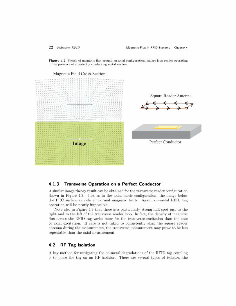
When a perfect electric conductor (PEC) is introduced to problem, there will bea dramatic reduction in magnetic field amplitudes close-in to the surface. Fieldstrength calculation in this situation is accomplished using image theory. Imagetheory states that the total field above a PEC is calculated by adding the free-spaceradiated fields of the square loop with its perfect image, reflected about the flatsurface of the PEC. This image has equal and opposite current flows which cancelall normal-components of magnetic field on the surface of the conductor. Thisbehavior is illustrated in Figure 4.2 for the axial configuration.

The presence of the metal is debilitating to RFID tag coupling because thereare no longer normal magnetic fields contributing to the total flux through the coil.Without normal flux, Faraday’s law predicts no voltage excitation around the coil.Only the marginal thickness of the dielectric substrate will allow a little magneticflux through the tag.

It is important to note that there are no real currents deep within the PECmedium; all of the cancelation currents are excited on the surface of the PEC.They simply mimic the equivalent behavior of a mirror-image source beneath theconductive medium. If the metal surface has finite conductivity, then the surfacecurrents imperfectly mimic this mirror source. To a rough approximation, we mayoffset the image current further from the surface by a distance equal to the skin

Section 4.1. Magnetic Field Modeling Durgin ECE 3065 Notes 21

Figure 4.1. Sketch of magnetic flux around a square loop operating in free space.

Magnetic Field Cross-Section

Square Reader Antenna

Inductive RFID Tag

Axial

Tran

sverse

Lateral

depth:

δ =1√

πfµσ(4.1.1)

where f is frequency (in Hz), µ is permeability (in H/m), and σ is conductivity (inS/m).

Based on this model, when the metal is a PEC, σ →∞ S/m and the skin depthapproaches zero; the image currents exactly reflect across the flat surface. When themetal becomes a dielectric material with σ → 0 S/m, the skin depth goes to infinityand the image is pushed so far away as to leave the surface fields identical to freespace. Finite conductivities represent in-between cases where the mirror current ispushed downward by a skin-depth (which can be shown to be the centroid depth ofthe surface currents).


Figure 4.2. Sketch of magnetic flux around an axial-configuration, square-loop reader operatingin the presence of a perfectly conducting metal surface.

Perfect Conductor



Image

4.1.3 Transverse Operation on a Perfect Conductor

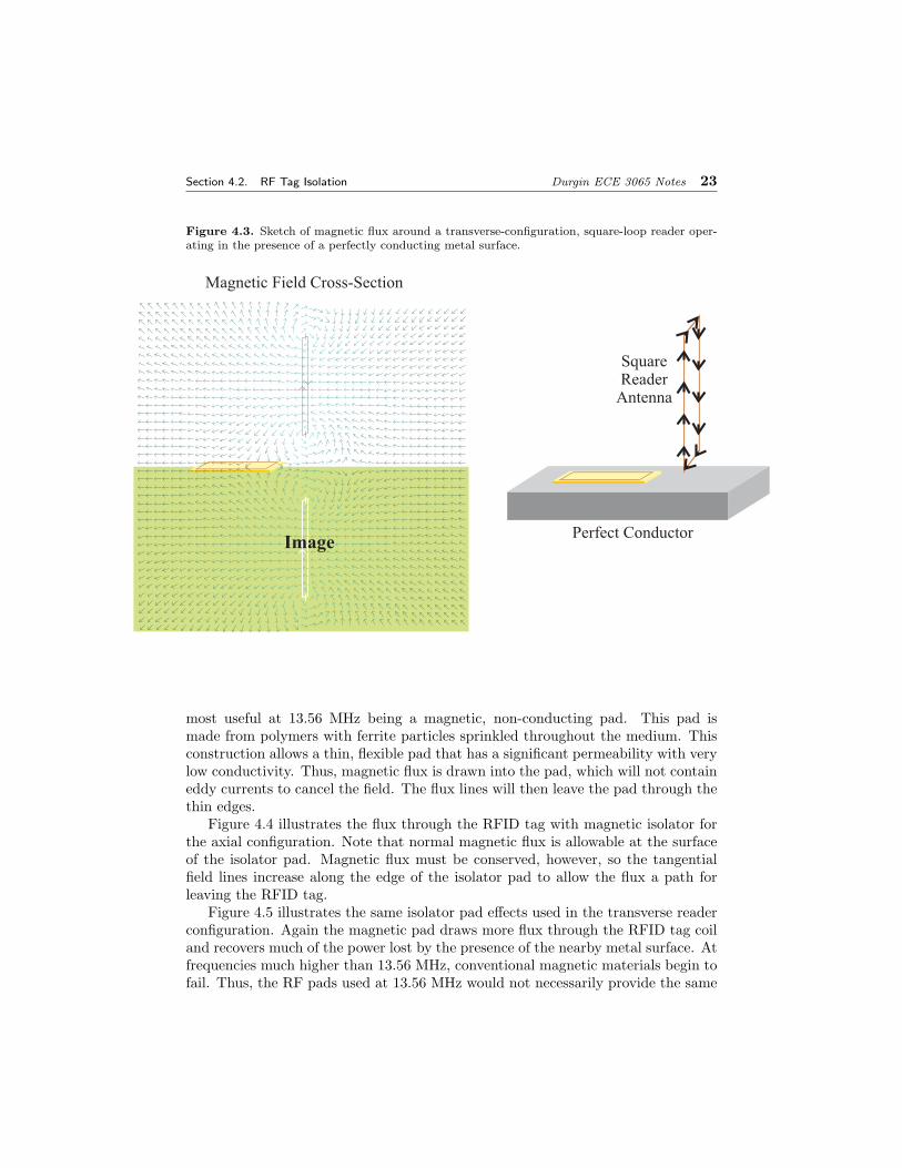
A similar image theory result can be obtained for the transverse reader configurationshown in Figure 4.3. Just as in the axial mode configuration, the image belowthe PEC surface cancels all normal magnetic fields. Again, on-metal RFID tagoperation will be nearly impossible.

Note also in Figure 4.3 that there is a particularly strong null spot just to theright and to the left of the transverse reader loop. In fact, the density of magneticflux across the RFID tag varies more for the transverse excitation than the caseof axial excitation. If care is not taken to consistently align the square readerantenna during the measurement, the transverse measurement may prove to be lessrepeatable than the axial measurement.

4.2 RF Tag Isolation

A key method for mitigating the on-metal degradations of the RFID tag couplingis to place the tag on an RF isolator. There are several types of isolator, the

Section 4.2. RF Tag Isolation Durgin ECE 3065 Notes 23

Figure 4.3. Sketch of magnetic flux around a transverse-configuration, square-loop reader oper-ating in the presence of a perfectly conducting metal surface.

ImagePerfect Conductor

SquareReader

Antenna


most useful at 13.56 MHz being a magnetic, non-conducting pad. This pad ismade from polymers with ferrite particles sprinkled throughout the medium. Thisconstruction allows a thin, flexible pad that has a significant permeability with verylow conductivity. Thus, magnetic flux is drawn into the pad, which will not containeddy currents to cancel the field. The flux lines will then leave the pad through thethin edges.

Figure 4.4 illustrates the flux through the RFID tag with magnetic isolator forthe axial configuration. Note that normal magnetic flux is allowable at the surfaceof the isolator pad. Magnetic flux must be conserved, however, so the tangentialfield lines increase along the edge of the isolator pad to allow the flux a path forleaving the RFID tag.

Figure 4.5 illustrates the same isolator pad effects used in the transverse readerconfiguration. Again the magnetic pad draws more flux through the RFID tag coiland recovers much of the power lost by the presence of the nearby metal surface. Atfrequencies much higher than 13.56 MHz, conventional magnetic materials begin tofail. Thus, the RF pads used at 13.56 MHz would not necessarily provide the same


protection at UHF or microwave frequencies.

Figure 4.4. Sketch of magnetic flux around an axial-configuration, square-loop reader operatingnear a perfect conducting metal surface with an RFID tag on a magnetic RF isolator pad.



Inductive RFID Tag

Conductor

MagneticIsolator

Conductor

4.3 Magnetic Flux Circuit Analysis

Aside from electrical circuits, there are actually many linear systems that can bemodeled with basic circuit theory. One such system is the flow of magnetic fluxthrough inhomogeneous materials. In this system, magnetic flux takes the place ofelectrical current in a conventional circuit; instead of voltage sources, the magneticcircuit is excited by magneto-motive force – a loop or coil of current that effectivelyenergizes the magnetic flux.

Because magnetic flux is neither created nor destroyed, it follows a Kirchhoffcurrent law just like electrical current. The net magnetic flux into any node withinthe circuit must be zero. Likewise, magneto-motive force satisfies the same con-servation properties of its counterpart, voltage, in electric circuits. When summedaround any arbitrary loop, the quantity we define as total magneto-motive forcemust equal zero in the magnetic circuit – just like Kirchhoff’s voltage law.

To complete the analogy, we need a physical quantity in a magnetic circuit toserve as an analogy to resistance. Then we can apply Ohm’s law and calculate howmagnetic flux might distribute itself in an inhomogeneous collection of materials.We will call this term reluctance, R, which will quantify how easily magnetic flux

Chapter 5

INDUCTIVE FIELDMODELING

If you are a technical reader that has made it this far in the text, there is no doubtthat you qualitatively understand the basic principle of power and informationcoupling in an inductive RFID system. It is another thing altogether to possess themental tools for quantitative analysis of these systems. Developing those tools isthe primary goal of this chapter.

31

32 Inductive RFID Inductive Field Modeling Chapter 5

5.1 Magnetic Field Modeling

5.1.1 Magnetic Field Around a Current Loop

We will model the excitation at the reader antenna as a square loop of current withside lengths L. This square will be centered at the origin and parallel with thexy-plane, as illustrated in Figure 5.1. Given a single line current I, we will usethe Biot-Savart relationship to calculate the ~H-field along the z-axis (~H(0, 0, z)).Off-axis behavior of the field is more difficult to calculate, but also unnecessaryif we assume that the RFID tag is roughly in the center of the reader antenna’sfield-of-view.

Figure 5.1. Magnetic flux flows through the square coil as a function of current and point ofobservation.

z

yx

L

Current, I

L

Here follows a step-by-step field analysis of the square current loop in Figure5.1.

1. The Biot-Savart relationship states that the total magnetic field due to acurrent in space is given by the following path integrations:

~H(~r) =∮

L

Idl × (~r − ~r′)4π‖~r − ~r′‖3 (5.1.1)

where ~r = xx + yy + zz is the observation point, ~r′ = x′x + y′y + z′z marksthe variables of integration, and I is the current in Amps. The integral inEquation (5.1.1) is taken around the closed current path. The first step is topick a differential element of integration:

Current in x-direction: dl = dx′x


Current in y-direction: dl = dy′y

This problem actually consists of 4 different current segments that travel intwo different directions. Two travel along x and two travel along y.

2. Next, pick the limits of integration:

∮

L

Idl × (~r − ~r′)4π‖~r − ~r′‖3 =

L/2∫

−L/2

Idx′ x× (zz − x′x + L2 y)

4π‖zz − x′x + L2 y‖3

︸︷︷︸Segment 1

+

L/2∫

−L/2

Idy′ y × (zz − L2 x− y′y)

4π‖zz − L2 x− y′y‖3


+

−L/2∫

L/2

Idx′ x× (zz − x′x− L2 y)

4π‖zz − x′x− L2 y‖3


+

−L/2∫

L/2

Idy′ y × (zz + L2 x− y′y)

4π‖zz + L2 x− y′y‖3


For this problem, our integral breaks into four pieces.

3. For observation on the z-axis, we will apply symmetry arguments. If all 4current segments are equal, then there should be no x or y components offield along the z axis. The two x-aligned segments will produce equal andopposite magnetic fields in the y-direction and the two y-aligned segmentswill produce equal and opposite magnetic fields in the x-direction. All four,however, will contribute equal amounts in the z-direction. Thus, we couldwrite:

~H(0, 0, z) = Hz(z)z Hz(z) = 4z ·L/2∫

−L/2


4π‖zz − x′x + L2 y‖3


4. Simplify the integral:

Hz = 4z ·L/2∫

−L/2


4π‖zz − x′x + L2 y‖3


=IL

2π

L/2∫

−L/2

dx′(z2 + L2

4 + x′2) 3

2


=IL

2π(z2 + L2

4

) x′√z2 + L2

4 + x′2

∣∣∣∣∣∣

x′= L2

x′=−L2

=IL

2π(z2 + L2

4

) L√z2 + L2

2

After all the simplifications, the final answer is

~H(0, 0, z) =I

2π(

z2

L2 + 14

)√z2 + L2

2

z (5.1.2)

Equation (5.1.2) is a key result the illustrates why the range of inductive RFID isso limited. For close-in operation (z ¿ L), the magnetic field becomes independentof z:

~H(0, 0, z) ≈ 2√

2I

πLz (5.1.3)

When the RFID tag is distant from the reader antenna (further than a side lengthL, such that z À L), the magnetic field falls off rapidly:

~H(0, 0, z) ≈ IL2

2πz3z (5.1.4)

The magnetic field – and mutual inductance – fall off as a function of 1/z3. Sincethe ability of the RFIC to reflect power back through the system varies with thesquare of mutual inductance, extra distance has a truly crippling effect on the powercoupling.

5.1.2 Field Strength vs. Distance

The current in the reader coil oscillates at f = 13.56 MHz and, following Faraday’sLaw, excites a voltage around the coil in the RFID tag. This voltage is then rectifiedby the chip to provide power to the memory and communication circuitry. Poweravailable for coupling into an inductive RFID will be proportional to the magnitude-squared of the magnetic field, ~H. With Nant turns in the reader antenna, we mayadapt Equation (5.1.2) for use along the z-axis:

~H(0, 0, z) =NantI

2π(

z2

L2 + 14

)√z2 + L2

2

z

Plotting the normalized power present in the magnetic field, ‖ ~H(0, 0, z)‖2/‖ ~H(0, 0, 0)‖2,produces the graph in Figure 5.3. Notice that when the card moves more than Laway from the reader coil, the energy density in the static magnetic field is reduced


Figure 5.2. To-scale image of a common 13.56 MHz RFIC card with insert removed.

Paper

Front

Clear

Plastic

Inset

Paper

Back

RFIC

Capacitive

Match

6-turn stampedaluminum coil


Figure 5.3. Graph of normalized power in the magnetic field for increasing tag-reader separationdistance.

Power vs. Range in Square Loop

-50

-45

-40

-35

-30

-25

-20

-15

-10

-5

0

0

0.2

0.4

0.6

0.8 1

1.2

1.4

1.6

1.8 2

2.2

2.4

2.6

2.8 3

Distance (z/L)

P/P

max

(dB

)

by a factor of 100! Since most readers cease free-space operation at approximately adistance L, me may assume that RFID systems can tolerate 20 dB of field-strengthloss compared to the ideal case (free-space operation with the RFID tag placed inthe center of the reader coil).

5.2 Inductance and Magnetic Coupling

5.2.1 Self Inductance

5.2.2 Mutual Inductance

Now we will estimate the mutual inductance between an RFID tag centered on thez-axis, parallel to the reader coil, and z units away from the plane of the coil. Wewill approximate the magnetic field as constant across the area of the RFID tag,

Section 5.2. Inductance and Magnetic Coupling Durgin ECE 3065 Notes 37

since the tag is relatively small compared to the reader antenna. In free space alongthe z-axis, we may write the magnetic flux density as

~B(0, 0, z) =NantIµ0

2π(

z2

L2 + 14

) √z2 + L2

2

z

Mutual inductance is defined as the ratio of total flux through both coils and thecurrent through the coils at the reader, M = Ψ21/I.

For a tag with Ntag turns, the total magnetic flux is approximately:

Ψ21 = NcA‖ ~B(0, 0, z)‖ =NantNtagAtagIµ0

2π(

z2

L2 + 14

) √z2 + L2

2

where Atag is the card area (approximately 0.0015 m2). Thus, mutual inductancein this system is

M =Ψ21

I=

NantNtagAtagµ0

2π(

z2

L2 + 14

)√z2 + L2

2

This allows us to construct Thevenin equivalent circuit models for the entire freespace system.

Figure 5.4. Circuit models for (left) self-inductive systems and (right) mutually-inductive sys-tems.

L1L1

V1V1 V2L2

M

++ +

-- -

I1I1 I2

Self-InductiveSystem

Mutually-InductiveSystem

5.2.3 Mutual Inductance Circuit Modeling

To create a system of equations that describes the mutually inductive system inFigure 5.4, we have to first recognize that there is an interdependence betweencurrents and voltages that do not exist in simpler circuit components. Namely, thecurrents flowing as I1 and I2 in the circuit of Figure 5.4 will both influence the


terminal voltages of port 1 and port 2. Working from the first-principles circuitmodeling time domain equations, we may write

V1 = L1dI1

dt−M

dI2

dtV2 = L2

dI2

dt−M

dI1

dt(5.2.1)

which would look like two stand-alone inductors if the second terms were removed(i.e. mutual inductance M vanished). When present, however, the second mutualinductance allows current I2 to excite additional voltage on port 1 and current I1

to excite additional voltage on port 2 consistent with Faraday’s law of induction.The sign is negative in the inductive term because the flux leaving one set of coilsenters into the second set of coils with opposite polarity of self-inductive fields.

There is a much more elegant way to write the interdependent set of relationshipsin Equation (5.2.1) using matrix notation. For a given frequency f , we may writethe matrix relationship between phasor voltages and currents as

[V1

V2

]= j2πf

[L1 −M−M L2

] [I1

I2

](5.2.2)

which is a simple linear system of algebraic equations. From this relationship, wecan construct a way to estimate how a load connected to port 2 influences theequivalent impedance seen at port 1 of the mutually inductive system.

If the equivalent resistance at port 1 of Figure 5.4 is given by Z1 = V1/I1,while the impedance connected to port 2 is given by Z2 = V2/I2, then these twoimpedances are related by the following equation:

Z1 =V1

I1= j2πfL1 +

4π2f2M2

Z2 + j2πfL2(5.2.3)

This relationship illustrates how a load of Z2 will reflect through the system andinfluence the Thevenin equivalent impedance of the system Z1. Notice that thereare two terms in Equation (5.2.3). The first term is a large self-inductive term thattypically dominates the total impedance Z1. Because typical mutual inductance ismuch smaller than the self-inductance terms (M2 ¿ L1L2), the right-hand termthat contains Z1 is much smaller – yet this is where the information exchange occurs.The next section illustrates how this circuit model may be used to analyze inductiveRFID systems.

5.3 Equivalent Circuit Model for the Basic RFID Card System

This section describes a first-principles equivalent circuit model for the RFID systemthat includes

5.3.1 Circuit Components of an RFID System

To construct an equivalent circuit model of an inductive RFID system, we need toadd some complexity to the simple mutual inductive system of Figure 5.4. To be

Section 5.3. Equivalent Circuit Model for the Basic RFID Card SystemDurgin ECE 3065 Notes 39

realistic, the model will need to incorporate the following physical attributes of anRF tag system:

Lant Antenna Self-Inductance: The antenna loop used to excite the RFID sys-tem will have a self-inductance term regardless of whether nearby RFID tagsare coupling into its wire currents.

Rant Antenna Loop Resistance: Any realistic antenna loop will have non-zeroresistance around its current path. The engineer always attempts to minimizethis term since it represents Ohmic losses in the system.

Vs RF Reader Voltage: This is the magnitude of the voltage source of theRFID reader, which may also be represented as a current source.

Rs RF Reader Resistance: This is the source resistance of the reader.

Cread Antenna Matching Capacitance: This capacitance, which is usually tun-able, helps to counter the antenna self-inductance and allows maximum powertransfer to and from coupled RF tags.

M Mutual Inductance: This is the mutual inductance between the RFID tagand the reader antenna, which depends on how much magnetic flux is sharedbetween the two. This is a function of orientation, tag-reader separation dis-tance/position, tag coil turns and geometry, antenna loop turns and geometry,and material environment.

Ltag Tag Self-Inductance: This term is the self-inductance of the RFID tag coil,independent of what reader may be coupling to the device.

Rcoil Tag Coil Resistance: The total resistance in the RFID tag coil representsOhmic losses along the tag’s main current path. The RFID tag always func-tions better when this term is minimized.

ZRFIC RFIC chip impedance: This is the Thevenin impedance of the RF inte-grated circuit connected to the RFID tag coil. Note that this value may changefor a single RFIC, depending on whether the chip is powering-up, absorbingpower in the steady-state, or modulating information back to the reader.

Cext Tag Matching Capacitance: This external matching capacitance is usedto match the tag’s RFIC with the inductive tag coil. If chosen correctly, thismatching capacitance will maximize the influence of the RFIC’s impedancechanges on the terminal impedance of the reader antenna.

Figure 5.5 illustrates the connectivity of these physical quantities. Armed with thiscircuit model, it will be possible to illustrate how an RFID system quantitativelyoperates. It will also be able to highlight critical design features of such a system.


Lant Ltag

CextCread

M RcoilRS

V tS( )

ZTh

ZRFIC

Rant

Reader Unit RFID Tag

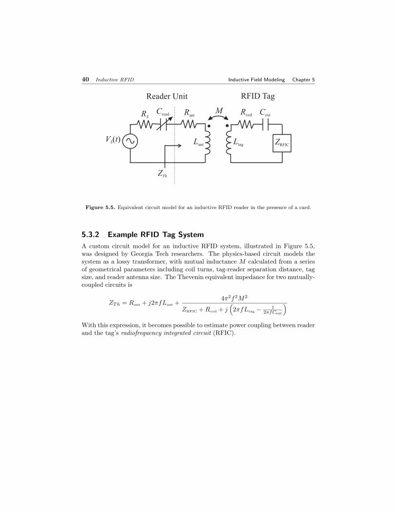
Figure 5.5. Equivalent circuit model for an inductive RFID reader in the presence of a card.

5.3.2 Example RFID Tag System

A custom circuit model for an inductive RFID system, illustrated in Figure 5.5,was designed by Georgia Tech researchers. The physics-based circuit models thesystem as a lossy transformer, with mutual inductance M calculated from a seriesof geometrical parameters including coil turns, tag-reader separation distance, tagsize, and reader antenna size. The Thevenin equivalent impedance for two mutually-coupled circuits is

ZTh = Rant + j2πfLant +4π2f2M2

ZRFIC + Rcoil + j(2πfLtag − 1

2πfCext

)

With this expression, it becomes possible to estimate power coupling between readerand the tag’s radiofrequency integrated circuit (RFIC).

Section 5.3. Equivalent Circuit Model for the Basic RFID Card SystemDurgin ECE 3065 Notes 41

Table 5.1. Table of typical circuit component values in a typical RFID system.

Var. Quantity Value Unitsf Frequency 13.56 MHz

Lant Antenna Loop Inductance 40.0 µHCread Antenna Tuning Capacitance X pFRant Antenna Loop Resistance X ΩLtag Tag Coil Inductance 7.8 µHCext Tag Matching Capacitance 24 pFRcoil Tag Coil Resistance 70 Ω

ZRFIC RFIC Impedance X Ω

MAGNETIC FLUX IN RFID SYSTEMS - Georgia …propagation.ece.gatech.edu/ECE3025/opencourse/MSF/...22...

Documents

Transcript of MAGNETIC FLUX IN RFID SYSTEMS - Georgia …propagation.ece.gatech.edu/ECE3025/opencourse/MSF/...22...