Magnetic Attitude Control for Spacecraft with Flexible ... · Magnetic Attitude Control for...
97
Magnetic Attitude Control for Spacecraft with Flexible Appendages by Julian Pierre Stellini A thesis submitted in conformity with the requirements for the degree of Master of Applied Science Graduate Department of Aerospace Science and Engineering University of Toronto Copyright c 2012 by Julian Pierre Stellini
Transcript of Magnetic Attitude Control for Spacecraft with Flexible ... · Magnetic Attitude Control for...

Magnetic Attitude Control forSpacecraft with Flexible
Appendages
by
Julian Pierre Stellini
A thesis submitted in conformity with the requirementsfor the degree of Master of Applied Science
Graduate Department of Aerospace Science and EngineeringUniversity of Toronto
Copyright c© 2012 by Julian Pierre Stellini
Magnetic Attitude Control for Spacecraft with
Flexible Appendages
Julian Pierre Stellini
Master of Applied Science
Graduate Department of Aerospace Science and Engineering
University of Toronto
2012
Abstract
The design of an attitude control system for a flexible spacecraft using magnetic actuation
is considered. The nonlinear, linear, and modal equations of motion are developed for a
general flexible body. Magnetic control is shown to be instantaneously underactuated,
and is only controllable in the time-varying sense. A PD-like control scheme is proposed
to address the attitude control problem for the linear system. Control gain limitations
are shown to exist for the purely magnetic control. A hybrid control scheme is also
proposed that relaxes these restrictions by adding a minimum control effort from an
alternate three-axis actuation system. Floquet and passivity theory are used to obtain
gain selection criteria that ensure a stable closed-loop system, which would aid in the
design of a hybrid controller for a flexible spacecraft. The ability of the linearized system
to predict the stability of the corresponding nonlinear system is also investigated.
ii
Acknowledgements
First and foremost, I would like to thank my mother. She has supported me without
question throughout my academic career and my entire life. She helped me get through
the late nights and times of confusion and frustration. I could not have done anything
without her.
I would like to thank Dr. Christopher Damaren for all of his guidance and support.
He is an undeniable expert in his field and I am honoured to have been able to work
under his supervision. His enthusiasm in his work made my time with him exciting and
rewarding. I appreciate all of his help.
I would also like to thank Dr. James Forbes and Ludwik Sobiesiak for all of their
help. They kept myself and the entire lab sane and friendly. They were always there to
share ideas and help me overcome any hurdles during my time at UTIAS.
I would like to acknowledge UTIAS itself, for providing me with a stimulating and
educational environment to work in. I always had the resources I needed at my disposal,
and I appreciate the friendly and fun atmosphere that it provided.
Lastly, I would like to thank all of my friends for being there when I needed them
most. It is very easy to get so caught up in work and school that you lose focus of all
the other important things in life and I am grateful for all the needed distractions and
good times that they have given me.
Julian Pierre Stellini
June 2012
iii

Contents
Abstract ii
Acknowledgements iii
Table of Contents v
List of Tables vi
List of Figures viii
1 Introduction 1
1.1 Literature Review . . . . . . . . . . . . . . . . . . . . . . . . . . . . . . . 3
1.2 Purpose . . . . . . . . . . . . . . . . . . . . . . . . . . . . . . . . . . . . 5
1.3 Thesis Overview . . . . . . . . . . . . . . . . . . . . . . . . . . . . . . . . 6
2 Background Concepts 8
2.1 Vectrix Notation . . . . . . . . . . . . . . . . . . . . . . . . . . . . . . . 8
2.1.1 Vector Dot and Cross Products . . . . . . . . . . . . . . . . . . . 9
2.1.2 Multiple Reference Frames and Rotation Matrices . . . . . . . . . 10
2.1.3 Angular Velocity and Vector Time Derivatives . . . . . . . . . . . 11
2.2 Attitude Representation . . . . . . . . . . . . . . . . . . . . . . . . . . . 12
2.2.1 Euler Angles . . . . . . . . . . . . . . . . . . . . . . . . . . . . . . 12
2.2.2 Quaternions . . . . . . . . . . . . . . . . . . . . . . . . . . . . . . 13
2.3 Stability Definitions . . . . . . . . . . . . . . . . . . . . . . . . . . . . . . 14
2.3.1 Lyapunov Stability . . . . . . . . . . . . . . . . . . . . . . . . . . 14
2.3.2 Input-Output Stability . . . . . . . . . . . . . . . . . . . . . . . . 15
2.4 Floquet Stability Theory . . . . . . . . . . . . . . . . . . . . . . . . . . . 16
2.5 Lyapunov Stability Theory . . . . . . . . . . . . . . . . . . . . . . . . . . 18
iv

2.5.1 Direct Method . . . . . . . . . . . . . . . . . . . . . . . . . . . . 18
2.5.2 Indirect Method . . . . . . . . . . . . . . . . . . . . . . . . . . . . 19
2.6 Passivity Theory . . . . . . . . . . . . . . . . . . . . . . . . . . . . . . . 19
3 Spacecraft Mechanics 21
3.1 Reference Frames . . . . . . . . . . . . . . . . . . . . . . . . . . . . . . . 21
3.2 Orbital Mechanics . . . . . . . . . . . . . . . . . . . . . . . . . . . . . . . 22
3.2.1 Orbit Orientation . . . . . . . . . . . . . . . . . . . . . . . . . . . 24
3.2.2 Orbital Elements . . . . . . . . . . . . . . . . . . . . . . . . . . . 25
3.3 Spacecraft Kinematics . . . . . . . . . . . . . . . . . . . . . . . . . . . . 27
3.4 Spacecraft Dynamics . . . . . . . . . . . . . . . . . . . . . . . . . . . . . 28
3.4.1 Rigid Spacecraft . . . . . . . . . . . . . . . . . . . . . . . . . . . 28
3.4.2 Flexible Spacecraft . . . . . . . . . . . . . . . . . . . . . . . . . . 30
3.4.3 Linearized Equations of Motion . . . . . . . . . . . . . . . . . . . 32
3.4.4 Modal Equations of Motion . . . . . . . . . . . . . . . . . . . . . 36
3.5 Archetypal Spacecraft/Orbit . . . . . . . . . . . . . . . . . . . . . . . . . 39
4 Magnetic Attitude Control 42
4.1 Magnetic Field Model . . . . . . . . . . . . . . . . . . . . . . . . . . . . 43
4.2 Controllability . . . . . . . . . . . . . . . . . . . . . . . . . . . . . . . . . 46
4.3 Hybrid PD-Like Control Law . . . . . . . . . . . . . . . . . . . . . . . . 48
5 Hybrid PD-Control Of Flexible Spacecraft 52
5.1 Floquet Stability Analysis . . . . . . . . . . . . . . . . . . . . . . . . . . 56
5.2 Hybrid Controller Gain Selection Criteria . . . . . . . . . . . . . . . . . . 62
5.3 Stability of the Nonlinear System . . . . . . . . . . . . . . . . . . . . . . 71
6 Conclusions 75
6.1 Future Work . . . . . . . . . . . . . . . . . . . . . . . . . . . . . . . . . . 77
References 79
Appendix A Geomagnetic Field Model Supplemental Calculations 82
Appendix B Hybrid Control Gain Selection For Rigid Spacecraft 84
Appendix C Floquet Stability Diagram for Rigid Spacecraft 88
v

List of Tables
3.1 Exact mode shape parameters for cantilevered beam. . . . . . . . . . . . 40
4.1 IGRF Coefficients for Epoch 2010. . . . . . . . . . . . . . . . . . . . . . . 44
5.1 Floquet stability prediction compared to nonlinear response. . . . . . . . 73
vi

List of Figures
1.1 A generic rigid spacecraft with two flexible beams attached. . . . . . . . 2
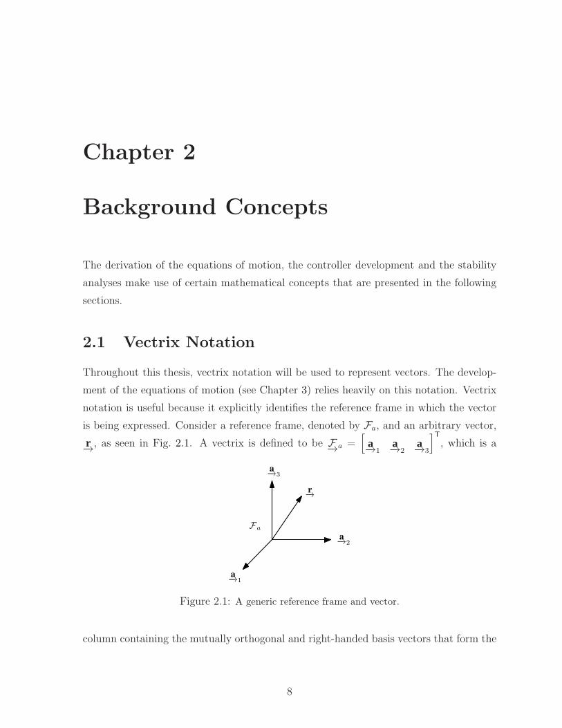
2.1 A generic reference frame and vector. . . . . . . . . . . . . . . . . . . . . 8
2.2 Block diagram of a system operator. . . . . . . . . . . . . . . . . . . . . 16
2.3 A generic feedback system. . . . . . . . . . . . . . . . . . . . . . . . . . . 20
3.1 The inertial and body-fixed frames. . . . . . . . . . . . . . . . . . . . . . 22
3.2 Polar coordinate system for spacecraft orbital position. . . . . . . . . . . 23
3.3 The geometry of an ellipse. . . . . . . . . . . . . . . . . . . . . . . . . . . 23
3.4 The orbital and inertial reference frames. . . . . . . . . . . . . . . . . . . 25
3.5 A generic rigid body. . . . . . . . . . . . . . . . . . . . . . . . . . . . . . 29
3.6 A generic unconstrained flexible body. . . . . . . . . . . . . . . . . . . . 31
3.7 A sample rigid spacecraft with two flexible beams attached. . . . . . . . . 40
4.1 An example of the geomagnetic field experienced in orbit. . . . . . . . . . 46
4.2 The cross-product relationship of the magnetic control torque. . . . . . . 47
4.3 A comparison of the geomagnetic field for polar and equatorial orbit. . . 48
4.4 A plot showing the existence of a gain limitation using PD-like control. . 50
5.1 Stability diagram obtained using Floquet theory. . . . . . . . . . . . . . . 57
5.2 Simulated spacecraft response demonstrating gain limitation. . . . . . . . 58
5.3 Interesting region of the Floquet stability diagram. . . . . . . . . . . . . 59
5.4 A plot showing the contribution of the flexible modes to the rigid ones. . 60
5.5 A plot illustrating the affect of flexibilty on the nonlinear system. . . . . 61
5.6 System response to purely magnetic control without elastic damping. . . 62
5.7 A plot showing a limitation of the Floquet analysis. . . . . . . . . . . . . 63
5.8 Block diagram for the flexible, hybrid-controlled system. . . . . . . . . . 66
5.9 Stability diagram obtained using passivity theory. . . . . . . . . . . . . . 67
vii

5.10 A plot illustrating the validity of the hybrid gain selection criteria. . . . . 68
5.11 A comparison of the attitude response for small/large initial conditions. . 72
5.12 An example of a stable and unstable nonlinear system response. . . . . . 74
B.1 Block diagram for a rigid, hybrid-controlled system. . . . . . . . . . . . . 86
C.1 Stability diagram for rigid spacecraft obtained using Floquet theory. . . . 88
C.2 Interesting region of the Floquet stability diagram for rigid spacecraft. . . 89
viii

Chapter 1
Introduction
The ability to control the attitude of spacecraft is a very important characteristic for any
space system to have. Spacecraft such as communications satellites rely on being able
to maintain line-of-sight with the earth as they traverse their orbits. Several methods
of providing active three-axis attitude control have been well documented and imple-
mented such as using reaction wheels, control-moment gyros, thrusters, etc. For small,
lightweight spacecraft that have very strict mass and power budgets with limited ability
to store fuel, the above techniques may be impractical to use.
Magnetic attitude control has recently been considered as a viable option for the
type of spacecraft described above. This method of control operates on the basis of
exploiting the interaction between the earth’s magnetic field and a set of three mutually
orthogonal electromagnetic actuators mounted on the spacecraft. These actuators could
be as simple as current loops aligned with the spacecraft body axes, which would create
three linearly independent dipole moments. This method of control is particularly suited
for low altitude orbits as the magnetic field is stronger in these regions and would allow for
a greater range of control torques [1]. The limitation of this technique is that the magnetic
control torque is only available perpendicular to the local geomagnetic field vector. This is
because the torque, τ−→(t), produced via an interaction between the actuator’s generated
dipole moment, m−→(t), and the magnetic field, b−→(t), is governed by the vector cross-
product
τ−→(t) = m−→(t)× b−→(t).
Thus, at most two axes are stabilizable at any given point in time, making the full three-
axis attitude stabilization problem unsolvable from a time-invariant point of view. This
1

Chapter 1. Introduction 2
fact is what poses the most difficulty when designing control laws for magnetic attitude
controllers. It is important to note however, that the geomagnetic field varies with time
along a spacecraft’s orbit, and [2] has shown that full control is possible if the variation
in the magnetic field is large enough (which is the case for near-polar orbits). Therefore,
magnetic attitude control is inherently a time-varying problem.
Lots of work has been done investigating various magnetic control schemes, and stabi-
lizing controllers exploiting the geomagnetic field have been successfully developed using
well-known methods such as optimal periodic control, linear-quadratic regulation (LQR)
techniques, and proportional/derivative (PD)-like control [3]. However, all of these mag-
netic control schemes are derived within the context of a rigid spacecraft. The topic
of attitude control systems for flexible spacecraft has been thoroughly studied as well,
and in this case controllers have also been successfully developed (i.e., see [4], [5] and
the references therein), but they involve types of actuation other than the geomagnetic
field and would therefore suffer the same disadvantages as described above if applied to
small/lightweight spacecraft.
There is a clear research gap: using magnetic actuation for the attitude control of
flexible spacecraft. Extending the magnetic control problem to the flexible case allows
for a broader class of spacecraft to be controlled by this method. For example, this
type of cotnrol would then be able to be used in controlling satellites with long, flexible
booms (on which items like scientific instruments, or solar panels may be mounted). The
general purpose of this thesis project is to commence bridging this gap by investigating
magnetic controller design methods for a specific subset of flexible spacecraft such as the
one mentioned above. In particular, the class of flexible spacecraft to be examined will
be limited to a rigid, central body with two flexible cantilever beams attached as shown
in Fig. 1.1.
F−→b
Rigid Body
Flexible Arm
ue1(y, t)
−ue2(y, t)
Flexible Arm
x
y
z
Figure 1.1: A generic rigid spacecraft with two flexible beams attached that will be used foranalysis and simulation purposes.

Chapter 1. Introduction 3
1.1 Literature Review
Before reviewing previous work done regarding this topic, it is important that the system
dynamics (including the interaction between the spacecraft and the geomagnetic field)
be controllable. An investigation on the controllability and accessibility conditions of a
nonlinear time-varying (NTV) spacecraft subject to magnetic attitude control was per-
formed in [6]. It is shown that the attitude dynamics are indeed controllable if the orbital
plane does not coincide with the geomagnetic equatorial plane and if the magnetic field is
periodic in time. See Chapter 4.2 for more specific information regarding controllability.
Since the literature regarding the attitude control of flexible spacecraft using magnetic
actuation is relatively scarce, the following review focuses on the techniques and control
schemes used for magnetic attitude control in the rigid spacecraft case. Looking at
how a rigid spacecraft may be controlled using these methods is an appropriate starting
point as they may possibly be extended to be applicable in the flexible case. A broad
exploration of the various approaches to magnetic attitude control for rigid spacecraft
can be found in [3], where linear methods (such as PD, H∞, and optimal control) and
nonlinear methods (such as magnetic predictive attitude control) are briefly compared
and contrasted.
Motivated by the Danish Ørsted satellite mission, [7] was able to develop a family of
controllers based on attitude and angular velocity feedback. The nonlinear, time-varying
system dynamics were considered in the controller design, and it was shown that the
control laws provided global three-axis attitude stabilization using magnetic torquers
only. The family of controllers were shown to be able to also provide joint control action
for satellite de-tumbling and nominal operation. It is important to note that there is
an error in this article, and its correction can be found in [8]. Also motivated by this
mission, [9] leveraged the periodic nature of the geomagnetic field for near-polar orbits
against the linear time-varying (LTV) dynamics to develop three types of controllers. Two
of them, finite and infinite horizon-based controllers, involves solving a periodic Riccati
equation, while the other was a constant-gain controller based on an approximation of
the monodromy matrix of the linearized system. A useful consequence of designing a
controller around a monodromy matrix is that a stability analysis using Floquet theory
can be easily applied.
The controllers proposed in [10] and [11] also exploit the periodic nature of the geo-
magnetic field. Asymptotic periodic LQR theory is used to design the controller in [10].

Chapter 1. Introduction 4
Integral action and saturation logic is included in the design in order to account for when
the magnetic actuators are providing the maximum magnetic moment that they are ca-
pable of. Simulation of the closed-loop LTV system exhibited robustness with respect to
modeling uncertainty and disturbance torques (such as residual dipoles). The controller
proposed in [11] uses periodic LQ optimal control techniques, and also relies on solving
a periodic Riccati equation. A unique feature of this controller is that it also includes
optimal estimation and compensation schemes for external disturbance rejection. The
disturbance estimation involves using a Kalman filter with output regulation strategies
similar to linear time-invariant (LTI) systems. In [12], H∞ control is used on LTV sys-
tems in order to design periodic controllers that perform well on the nonlinear system
and are also robust against large disturbance torques.
A PD-like control law is featured in the controllers designed in [13–16]. Static and
dynamic attitude and rate feedback is used to provide almost global attitude stabilization.
Reference [13] also looks at actuator saturation constraints and contingencies for when
one or more of the actuators becomes unavailable. Reference [14] proposes an adaptive
version of the PD-like control law, and uses a generalized averaging theory to prove
stability. In [15], it is demonstrated that stabilization without the rate feedback is also
possible with a minor adaptation to the control law. Note that the stability proofs
for all of these PD-like control laws rely on the generalized averaging theory described
in [17], which imposes mathematical limits on the gains in all of the controllers. These
mathematical limits can be shown to have a physical manifestation. This is a very
important result as it places restrictions on the performance of this simple and easy-to-
implement control strategy. Also, it is shown in [15] that the application of this relatively
simple control strategy requires that a matrix involving the geomagnetic field be positive
definite, restricting the use of this type of controller to non-equatorial orbits.
A family of optimal control programs called RIOTS is used by [18] to implement
a time-optimal open-loop controller. Using RIOTS allowed for designing a controller
around the NTV spacecraft dynamics with constrained inputs. A sub-optimal model
predictive feedback closed-loop control scheme is also proposed by [18], which attempts
to track a pre-calculated optimal trajectory. These controllers address the slow conver-
gence to equilibria inherent in other magnetic attitude control schemes, and can therefore
be used for time critical maneuvering. In [19], a discrete-time approach was taken. Three
optimal discrete-time controllers were proposed: a periodic optimal state feedback con-
troller, a predictive magnetic controller, and a fixed-structure projection-based controller.

Chapter 1. Introduction 5
Reference [20] proposes magnetic attitude control designs for the REIMEI microsatellite
similar to some of those already discussed. The novel contribution in [20] is an implemen-
tation of a residual magnetic moment observer and its feed-forward cancellation, which
suggests similar approaches may be taken for other disturbance torques. In [21] an LQR
control method (based on solving an algebraic Riccati equation) designed around the
linearized system is compared to another approach relying on the solution of a state-
dependent Riccati equation (using a state-dependent coefficient method) design around
the nonlinear system. It is shown that the latter method was found to be more robust
and stable as it includes the use of a variable-gain feedback.
Partial magnetic actuation has also been considered by some. These techniques in-
volve having the magnetic torquers as the main control source as well as other active
actuators, such as reaction wheels or thrusters, for support. Reference [22] shows that
using partial magnetic actuation can allow for the spacecraft dynamics to be treated as
an LTI system. The proposed control law is then a simple state feedback. Reference [22]
also addresses the inherent control allocation problem for optimum performance. Two
approaches were considered: a direct approach where the supporting actuators would
only provide control for the axis that the magnetic actuator can’t affect, and a quadratic
programming decision method that involves solving an optimization program. In [23] a
geometric approach is followed for the control allocation problem. A systematic way of
allocating the two control torques such that they do not overlap and potentially negate
each other is described. Another partial magnetic actuation strategy is proposed in [24],
where the PD-like control law of [16] is combined with a similar law for the other actua-
tion system. It is shown how the limitation on the attitude gain (proved in [16]) can be
alleviated with a minimum level of contribution from the supporting actuators.
The PD-like control strategy in [16] was shown to maintain its stability properties
when applied to a flexible spacecraft in [25]. However, this controller is still subject to the
gain limitation setbacks described above. It also does not use any information regarding
the flexible dynamics of the system, and its adequate performance suggests that there is
much room for improvement.
1.2 Purpose
The purpose of this thesis is to investigate controller design methods for the attitude
control of spacecraft with flexible appendages, using magnetic actuation. Certain con-

Chapter 1. Introduction 6
trollers designed for a rigid spacecraft will be extended to the flexible case. Conditions
for the stability of the resulting closed-loop systems will be investigated, thereby provid-
ing insight into the controller design. The analysis and design methods will be based on
the linearized dynamics, and the performance of the resulting controller on the nonlinear
system will be investigated.
1.3 Thesis Overview
Chapter 1 provides a brief introduction to the importance and relevance of exploiting
the earth’s magnetic field to control the attitude of spacecraft in general. The general
purpose and scope of the work done in this thesis is also explained. A review of the
relevant literature for this topic is provided as well.
Chapter 2 summarizes the background mathematics and concepts relevant to the
work done in this thesis: using vectrix notation to represent vectors and vector operations;
spacecraft attitude representation using rotation matrices, Euler angles, and quaternions;
definitions of input-output and Lyapunov stability; and various stability theories such as
Lyapunov, Floquet, and passivity theory.
Chapter 3 provides a description of the relevant frames of reference, the orbital dy-
namics of a spacecraft orbiting the earth, and the mechanics (kinematics and dynamics)
of a general flexible and rigid spacecraft. The nonlinear and linear equations of motion
are derived. Modal analysis is performed on the linearized system and the equivalent
modal equations of motion are also developed.
Chapter 4 provides a more in-depth look at magnetic attitude control. The model used
to represent the earth’s magnetic field is included, as well as a summary of an investigation
into the controllability of spacecraft using this type of actuation. Approaches to magnetic
control relevant to this thesis are introduced and explored.
In Chapter 5, a hybrid PD-like control law is proposed and conditions under which
the closed-loop system is stable are investigated. A stability map for the controller is
obtained using Floquet theory. Passivity theory is used to obtain controller gain selection
criteria. The effect of the elastic properties of the flexible spacecraft on its stability are
also considered. The performance of the control law on the nonlinear system is explored
as well.
Finally, Chapter 6 summarizes the work done in the preceding chapters, and proposes
potential areas to explore in order to expand the results of this thesis. Supplementary

Chapter 1. Introduction 7
material required for a better understanding of some of the topics discussed in this thesis
are included in the appendices.
Chapter 2
Background Concepts
The derivation of the equations of motion, the controller development and the stability
analyses make use of certain mathematical concepts that are presented in the following
sections.
2.1 Vectrix Notation
Throughout this thesis, vectrix notation will be used to represent vectors. The develop-
ment of the equations of motion (see Chapter 3) relies heavily on this notation. Vectrix
notation is useful because it explicitly identifies the reference frame in which the vector
is being expressed. Consider a reference frame, denoted by Fa, and an arbitrary vector,
r−→, as seen in Fig. 2.1. A vectrix is defined to be F−→a =[
a−→1
a−→2
a−→3
]T
, which is a
r−→
a−→1
a−→2
a−→3
Fa
Figure 2.1: A generic reference frame and vector.
column containing the mutually orthogonal and right-handed basis vectors that form the
8

Chapter 2. Background Concepts 9
reference frame Fa. The vector r−→ can be then be expressed as
r−→ = r1 a−→1
+ r2 a−→2
+ r3 a−→3
=[
a−→1
a−→2
a−→3
]
r1
r2
r3
= F−→aTr
= rTF−→a,
where r =[
r1 r2 r3
]T
, r ∈ R3×1 is a column matrix containing the scalar components of
r−→ as expressed in Fa. Any equation or operation involving vectors can then be described
in terms of matrices, so long as all of the vectors are expressed in the same frame. More
detailed information regarding vectrix notation can be found in the appendices of [26].
2.1.1 Vector Dot and Cross Products
Given the vectrix notation described in Chapter 2.1, both the dot and cross products
between two vectors can be easily described in terms of matrix multiplication. Consider
two vectors, r−→ = F−→aTr and s
−→= F−→a
Ts (note how both are expressed in the same
reference frame). The dot product is then given by
r−→ · s−→
=[
r1 r2 r3
]
a−→1
a−→2
a−→3
·[
a−→1
a−→2
a−→3
]
s1
s2
s3
=[
r1 r2 r3
]
a−→1
· a−→1
a−→1
· a−→2
a−→1
· a−→3
a−→2
· a−→1
a−→2
· a−→2
a−→2
· a−→3
a−→3
· a−→1
a−→3
· a−→2
a−→3
· a−→3
s1
s2
s3
= rT1s
= rTs
= sTr ,

Chapter 2. Background Concepts 10
where 1 is used to denote the identity matrix. Similarily, the cross product is given by
r−→× s−→
=[
r1 r2 r3
]
a−→1
× a−→1
a−→1
× a−→2
a−→1
× a−→3
a−→2
× a−→1
a−→2
× a−→2
a−→2
× a−→3
a−→3
× a−→1
a−→3
× a−→2
a−→3
× a−→3
s1
s2
s3
=[
r1 r2 r3
]
0−→ a−→3
− a−→2
− a−→3
0−→ a−→1
a−→2
− a−→1
0−→
s1
s2
s3
=[
a−→1
a−→2
a−→3
]
0 −r3 r2
r3 0 −r1
−r2 r1 0
s1
s2
s3
= F−→aTr×s
= F−→aT(−s×r
),
where
r× =
0 −r3 r2
r3 0 −r1
−r2 r1 0
is a skew-symmetric matrix ((r×)T = −r×) that constructs the components of the cross
product.
2.1.2 Multiple Reference Frames and Rotation Matrices
Consider two reference frames denoted by F−→a and F−→b. The situation often arises when
a vector r−→ is given in one frame, yet its representation in the other frame is required.
Vectrix notation provides a simple way of resolving this issue. First, it is evident that
r−→ = F−→aTra = F−→b
Tr b and so
F−→bTr b = F−→a
Tra
F−→b · F−→bTr b = F−→b · F−→a
Tra
r b = Cbara,

Chapter 2. Background Concepts 11
where
Cba = F−→b · F−→aT
=
b−→1
· a−→1
b−→1
· a−→2
b−→1
· a−→3
b−→2
· a−→1
b−→2
· a−→2
b−→2
· a−→3
b−→3
· a−→1
b−→3
· a−→2
b−→3
· a−→3
.
This matrix is a direction cosine matrix describing the rotation between the two reference
frames. It belongs to SO(3), which is the group of 3 × 3 orthogonal rotation matrices
with determinant equal to unity. Thus, Cba takes a vector expressed in Fa and rotates it
into Fb.
2.1.3 Angular Velocity and Vector Time Derivatives
Suppose that Fb is rotating with respect to Fa, and let the angular velocity of Fb with
respect to Fa be denoted by ω−→ba. The magnitude of the angular velocity represents the
rate of rotation, and its unit vector represents the instantaneous axis of rotation.
For ω−→ba6= 0−→, the motion experienced in either frame is not the same. Let the vector
time derivative as seen in Fa be denoted by (·) and that in Fb by (). As defined, it is
clear that F−→a =
F−→b= 0−→. As for the derivative of Fb as seen in Fa, it can be shown using
vector calculus that [26]
F−→bT
= ω−→ba× F−→b
T.
Now consider a vector r−→; its time derivatives as seen in either frame is
r−→ = F−→aT
ra + F−→aTra = F−→a
Tra
r−→ =
F−→b
T
r b + F−→bT
r b= F−→bTr b,
noting that the vector time derivative of a column matrix is simply the regular time
derivative independent of frame, and is also denoted by (·). Using these relationships,
one can obtain the derivative of a vector in one frame in terms of the motion in the other

Chapter 2. Background Concepts 12
frame since
r−→ = F−→aTra = F−→b
Tr b + F−→bT
r b
= F−→bTr b + ω−→ba
× F−→bTr b
= F−→bT(r b + ω×
bar b).
2.2 Attitude Representation
Consider the rotation matrix Cba in Chapter 2.1.2. If F−→a and F−→b are chosen such that
they are inertial and body-fixed (i.e., as in Chapter 3.1), respectively, then Cba can be
considered as representing the orientation (or attitude) of the body with respect to inertial
space. The rotation matrix has nine entries, and so at first it would appear that there are
nine independent variables needed to describe the rotation. However, Euler’s Theorem
of Rotations says that any rotation can be described by defining an axis represented by
the unit vector a−→, about which the body is rotated, and an angle φ ∈ R, denoting the
degree of rotation [26]. These two variables can be combined into a single vector, ν−→,
where
ν−→ = φ a−→.
Thus, any rotation can be described by the vector ν−→, where its magnitude is the angle of
rotation, and its unit vector is the rotation axis. In three-dimensional space a minimum
representation of Cba would require only three parameters.
Many rotation matrix parameterizations exist, and choosing a suitable one depends
on the context of the problem. Some of the more common parameterization used in
spacecraft kinematics are Euler angles, Rodrigues parameters, and quaternions [26].
2.2.1 Euler Angles
An intuitive parameterization of the rotation matrix are Euler angles. First, it is noted
that SO(3) is closed under matrix multiplication, and that successive rotations can be
obtained simply by multiplying rotation matrices together. Furthermore, any rotation
can be decomposed into three successive principle rotations about a principal axes. A
principle rotation matrix, Ci (θ), denotes a rotation of θ radians about the i-th axis. Note

Chapter 2. Background Concepts 13
that
Ci (θ) =
1 0 0
0 cos(θ) sin(θ)
0 − sin(θ) cos(θ)
describes a rotation of θ radians about the i−→ axis, where i−→ = span
[
1 0 0]T
.
In this way an ijk-Euler angle, denoted by θ =[
θ1 θ2 θ3
]T
, represents the rotation
matrix
Cba (θ) = Ck (θ1)Cj (θ2)Ci (θ3) .
For example, letting 1−→, 2−→, 3−→ equal i−→, j−→
, k−→ respectively, a 321-Euler angle θ would
represent the following sequence of rotations:
1. A rotation of θ3 about the original (i.e., F−→a) 3−→ axis.
2. A rotation of θ2 about the intermediate 2−→ axis.
3. A rotation of θ1 about the transformed (i.e., F−→b) 1−→ axis.
The resulting rotation matrix would then look like
Cba (θ) = C1 (θ1)C2 (θ2)C3 (θ3)
=
c2c3 c2s3 −s2
s1s2c3 − c1s3 s1s2s3 + c1c3 s1c2
c1s2c3 + s1s3 c1s2s3 − s1c3 c1c2
,
where si = sin(θi), and ci = cos(θi). It is important to note that this particular Euler
angle representation has a singularity when θ2 =π2. When this occurs, θ1 and θ3 describe
the same degree of freedom, making it impossible for them to be uniquely determined.
Singularities like this occur with all Euler angle sequences, as well as with most other
parameterizations such as the Rodrigues parameters. Choice of Euler angle sequence
then becomes very important depending on the application, and care must be taken to
ensure that the system avoids those singularities.
2.2.2 Quaternions
A singularity-free parameterization of the rotation matrix can be obtained when using
quaternions (also called Euler parameters). This representation relies on the axis-angle
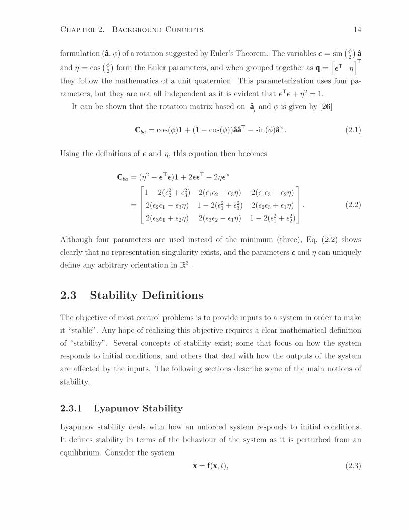
Chapter 2. Background Concepts 14
formulation (a, φ) of a rotation suggested by Euler’s Theorem. The variables ǫ = sin(φ2
)a
and η = cos(φ2
)form the Euler parameters, and when grouped together as q =
[
ǫT η
]T
they follow the mathematics of a unit quaternion. This parameterization uses four pa-
rameters, but they are not all independent as it is evident that ǫTǫ+ η2 = 1.
It can be shown that the rotation matrix based on a−→
and φ is given by [26]
Cba = cos(φ)1+ (1− cos(φ))aaT − sin(φ)a×. (2.1)
Using the definitions of ǫ and η, this equation then becomes
Cba = (η2 − ǫTǫ)1+ 2ǫǫT − 2ηǫ×
=
1− 2(ǫ22 + ǫ23) 2(ǫ1ǫ2 + ǫ3η) 2(ǫ1ǫ3 − ǫ2η)
2(ǫ2ǫ1 − ǫ3η) 1− 2(ǫ21 + ǫ23) 2(ǫ2ǫ3 + ǫ1η)
2(ǫ3ǫ1 + ǫ2η) 2(ǫ3ǫ2 − ǫ1η) 1− 2(ǫ21 + ǫ22)
. (2.2)
Although four parameters are used instead of the minimum (three), Eq. (2.2) shows
clearly that no representation singularity exists, and the parameters ǫ and η can uniquely
define any arbitrary orientation in R3.
2.3 Stability Definitions
The objective of most control problems is to provide inputs to a system in order to make
it “stable”. Any hope of realizing this objective requires a clear mathematical definition
of “stability”. Several concepts of stability exist; some that focus on how the system
responds to initial conditions, and others that deal with how the outputs of the system
are affected by the inputs. The following sections describe some of the main notions of
stability.
2.3.1 Lyapunov Stability
Lyapunov stability deals with how an unforced system responds to initial conditions.
It defines stability in terms of the behaviour of the system as it is perturbed from an
equilibrium. Consider the system
x = f(x, t), (2.3)

Chapter 2. Background Concepts 15
where x(t) ∈ Rn, t ∈ R
+, and f : Rn × R+ → R
n. The state x0 is an equilibrium of
Eq. (2.3) if f(x0, t) = 0. This equilibrium is said to be stable (or L-stable) if for any
ǫ > 0, there exists a δ > 0 such that
‖x(0)− x0‖ < δ ⇒ ‖x(t)− x0‖ < ǫ .
Furthermore, the equilibrium x0 is said to asymptotically stable if it is stable and there
exists a δ > 0 such that
‖x(0)− x0‖ < δ ⇒ x(t) → x0 as t→ ∞.
The equilibrium is globally asymptotically stable if it is stable and for any δ > 0, x(t) → x0
as t→ ∞. Finally, the equilibrium is considered unstable if it is not stable.
2.3.2 Input-Output Stability
Input-output (I/O) stability aims at describing how the inputs to a system affect the
outputs. There are many different classes of inputs that can potentially be applied to a
system, so for the purposes of this thesis admissible inputs will be required to belong to
the L2-space of functions defined by
L2 = u(t) | ‖u(t)‖2 <∞ ,
where ‖u(t)‖2 is the 2-norm of a vector function of time and is given as
‖u(t)‖2 =
√∫
∞
0
uT(t)u(t) dt.
Functions belonging to L2 can be thought of as having “finite energy”. In describing
I/O-stability it will be useful to define the truncation of a function as
uT (t) =
u(t) if t ≤ T
0 if t > T.

Chapter 2. Background Concepts 16
This gives rise to the idea of an extended L2-space denoted by
L2e = u(t) | uT (t) ∈ L2, 0 < T <∞ .
A “system” can mathematically be described as a mapping (or operator) G : L2e → L2e
which maps the input functions u(t) to its output functions y(t). This mapping operation
can be written as y = Gu, and described in block diagram form as seen in Fig. 2.2. The
u yG
Figure 2.2: Block diagram of a system operator.
system operator G is said to be input-output stable, or L2-stable, if
u ∈ L2 ⇒ y ∈ L2,
which can be interpreted as: if a finite energy input acts on the system, the corresponding
output also has finite energy. It is important to note that it can be shown that for any
function v ∈ L2, if v ∈ L2 then limt→∞v(t) = 0. This result links the concepts of
input-output stability with Lyapunov stability.
2.4 Floquet Stability Theory
Floquet theory provides a convenient way to determine the stability of a linear periodic
system of the form
x = A(t)x, (2.4)
where A(t + T ) = A(t). This section provides a summary of this theory as described
in [26] and [27].
Letting Φ(t, t0) represent the principal fundamental matrix solution of Eq. (2.4), it is
clear that
Φ(t, t0) = A(t)Φ(t, t0),
and it can be shown that the columns of Φ are linearly independent, thereby forming a
Chapter 2. Background Concepts 17
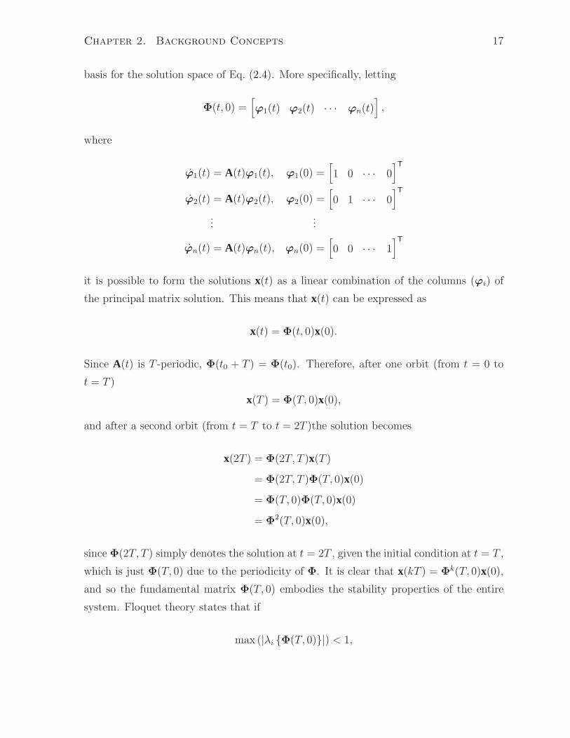
basis for the solution space of Eq. (2.4). More specifically, letting
Φ(t, 0) =[
ϕ1(t) ϕ2(t) · · · ϕn(t)]
,
where
ϕ1(t) = A(t)ϕ1(t), ϕ1(0) =[
1 0 · · · 0]T
ϕ2(t) = A(t)ϕ2(t), ϕ2(0) =[
0 1 · · · 0]T
......
ϕn(t) = A(t)ϕn(t), ϕn(0) =[
0 0 · · · 1]T
it is possible to form the solutions x(t) as a linear combination of the columns (ϕi) of
the principal matrix solution. This means that x(t) can be expressed as
x(t) = Φ(t, 0)x(0).
Since A(t) is T -periodic, Φ(t0 + T ) = Φ(t0). Therefore, after one orbit (from t = 0 to
t = T )
x(T ) = Φ(T, 0)x(0),
and after a second orbit (from t = T to t = 2T )the solution becomes
x(2T ) = Φ(2T, T )x(T )
= Φ(2T, T )Φ(T, 0)x(0)
= Φ(T, 0)Φ(T, 0)x(0)
= Φ2(T, 0)x(0),
since Φ(2T, T ) simply denotes the solution at t = 2T , given the initial condition at t = T ,
which is just Φ(T, 0) due to the periodicity of Φ. It is clear that x(kT ) = Φk(T, 0)x(0),
and so the fundamental matrix Φ(T, 0) embodies the stability properties of the entire
system. Floquet theory states that if
max (|λi Φ(T, 0)|) < 1,

Chapter 2. Background Concepts 18
where λi is an eigenvalue of Φ(T, 0), then Eq. (2.4) is asymptotically stable.
2.5 Lyapunov Stability Theory
Lyapunov stability theory deals with describing the stability of “unforced” systems of
the form
x = f(x, t). (2.5)
It also provides a means of inferring the stability of an equilibrium of a nonlinear system
by looking at the stability of the corresponding linear system. This section summarizes
the Lyapunov theory discussed in [26] and [28].
2.5.1 Direct Method
This method provides a means of determining the stability of a system by examining
the existence of a particular function V (x, t), called the Lyapunov function, that has
certain characteristics. This Lyapunov function is akin to a storage function. Consider
the system described by Eq. (2.5), with x(0) = x0 as an equilibrium (i.e., f(x0) = 0).
Also, it is assumed that x0 = 0 (which can be achieved via a coordinate transformation).
The equililibrium x0 of Eq. (2.5) is
• stable if there exists a C1 locally positive definite function V (x, t) such that V (x, t)
is locally negative semi-definite for all t ≥ 0;
• asymptotically stable if there exists a C1 locally positive definite function V (x, t)
such that V (x, t) is locally negative definite for all t ≥ 0;
• globally asymptotically stable if there exists a C1, positive definite, and radially
unbounded function V (x, t) such that V (x, t) is negative definite for all t ≥ 0.
In the conditions above, the time derivative of V are taken to be along the trajectories
of Eq. (2.5). That is,
V (x, t) =∂V
∂t+∂V
∂xTf(x, t).
It is important to note that this method only gives sufficient conditions for stability
meaning that even if a Lyapunov function doesn’t exist for the system, it may still be
stable.

Chapter 2. Background Concepts 19
2.5.2 Indirect Method
This method provides a way to determine (albeit in a limited manner) the stability of an
equilibrium of a nonlinear system by looking at the stability of its corresponding linear
system. Consider Eq. (2.5), also with x(0) = x0 as an equilibrium. Letting x = x0 + δx
and neglecting higher order terms in the corresponding Taylor expansion of Eq. (2.5),
the linearized system can be written as
δx = Aδx, (2.6)
where
A =∂f∂xT
∣∣∣∣x=x0
is the Jacobian of the nonlinear system about the equilibrium x0. Lyapunov’s Indirect
Method states that if the equilibrium δx = 0 of Eq. (2.6) is
• asymptotically stable then x0 is a locally asymptotically stable equilibrium of the
nonlinear system;
• unstable then x0 is an unstable equilibrium of the nonlinear system;
• stable then no conclusion can be inferred regarding the nonlinear system.
2.6 Passivity Theory
Passivity theory focuses on describing relationships between the inputs and outputs of
a given system. Thus, it provides a means of controller design ensuring input-output
stability. This section provides a summary of passivity theory as given in [28] and [29].
Consider a square system denoted by
y = Gu,
where u ∈ R, y ∈ R, and G : L2e → L2e. Note that, as in Chapter 2.3.2, G is considered
to be an operator that maps the system’s inputs, u, to its outputs, y. The operator G is
said to be passive if, for any u ∈ L2e, and for any T ≥ 0,
∫ T
0
uT (Gu) dt =∫ T
0
yTu dt ≥ 0.

Chapter 2. Background Concepts 20
Furthermore, the operator G is said to be strictly passive if, for any u ∈ L2e, and for any
T ≥ 0, there exists ǫ > 0 such that
∫ T
0
uT (Gu) dt =∫ T
0
yTu dt ≥ ǫ
∫ T
0
uTu dt.
The passivity theorem describes the input-output stability of the interconnection between
a passive and strictly passive system. Consider the feedback system given in Fig. 2.3.
The passivity theorem states that if G is passive and H is strictly passive, then the
+
−
u y1
y2
G
H
e
Figure 2.3: A generic, closed-loop feedback system.
feedback system is L2-stable. This implies that if the passivity theorem holds for this
system, then u ∈ L2 ⇒ y1 ∈ L2. See [29] for more detailed information regarding the
passivity theorem.

Chapter 3
Spacecraft Mechanics
Knowledge of how a system moves and responds under the influence of external forces
may give insight into controller design. This chapter aims to describe the mechanics of
a generic spacecraft system.
3.1 Reference Frames
There are two types of reference frames that are particularly useful in the context of
spacecraft attitude control: an inertial one and a body-fixed one. The inertial (non-
rotating) reference frame will be denoted by F−→i =[
i−→1i−→2
i−→3
]T
and is taken to be
the geocentric equatorial coordinate system. The origin of this frame is located at the
centre of the earth. The basis vector i−→1points in the direction of the vernal equinox
(also called Aries, or à), and i−→3points towards the geographical north pole. The
remaining basis vector lies in the equatorial plane with i−→1, such that it completes the
right-handed coordinate system. This particular inertial reference frame coincides with
the one that is typically used to describe the mechanics of a spacecraft orbiting the earth.
The second reference frame of interest is an orthogonal and right-handed one attached
to the spacecraft body itself, with the origin located at the body’s centre of mass. It is
denoted by F−→b =[
b−→1
b−→2
b−→3
]T
, and its relationship to the inertial frame is shown in
Fig. 3.1 (note that the vector r−→ in Fig. 3.1 describes the position of the centre of mass
of the spacecraft with respect to the centre of mass of the earth).
With these choices of reference frames the attitude of the spacecraft can then be rep-
resented by the rotation matrix Cbi, as described in Chapter 2.2. Also, it is important to
note that in subsequent chapters (particularly Chapters 3.3 and 3.4), the time derivative
21

Chapter 3. Spacecraft Mechanics 22
i−→1
i−→3
i−→2
à
b−→3
b−→2
b−→1
Earth
Spacecraft
Equator
North Pole
r−→
Figure 3.1: The inertial and body-fixed frames.
as seen in F−→i will be denoted by (·) and that as seen in F−→b by ().
3.2 Orbital Mechanics
Since the geomagnetic field vector experienced by a spacecraft depends on the spacecraft’s
location with respect to the centre of the earth (see Chapter 4.1), it is necessary, at least
for simulation purposes, to be able to calculate orbital positions as a function of time. To
this end, a brief summary of orbital dynamics will be presented (based on the material
in [30]).
The equations of motion describing the orbit shape can be found by examining the
two-body problem of classical mechanics. Taking into account that, of the two-bodies in
question (the earth and the spacecraft), the earth’s mass is considered to be much larger
than that of the spacecraft, the earth’s approximate position remains at one of the focal
points of the resulting orbit shape. It can also be shown that the angular momentum
per unit mass, h−→, of the system is constant. Since h−→ = r−→× r−→, the motion is confined
to a plane perpendicular to the angular momentum. Note that r−→ refers to the position
of the centre of mass of the spacecraft with respect to the centre of mass of the earth
(as in Fig. 3.1). With this in mind, the reference frames in Fig. 3.2 introduce a way of
describing r−→ in polar coordinates. The equations of motion then reduce to
Chapter 3. Spacecraft Mechanics 23
Spacecraft
Earth
Orbit
θ
θ
1−→1
2−→1
1−→2
2−→2
r−→
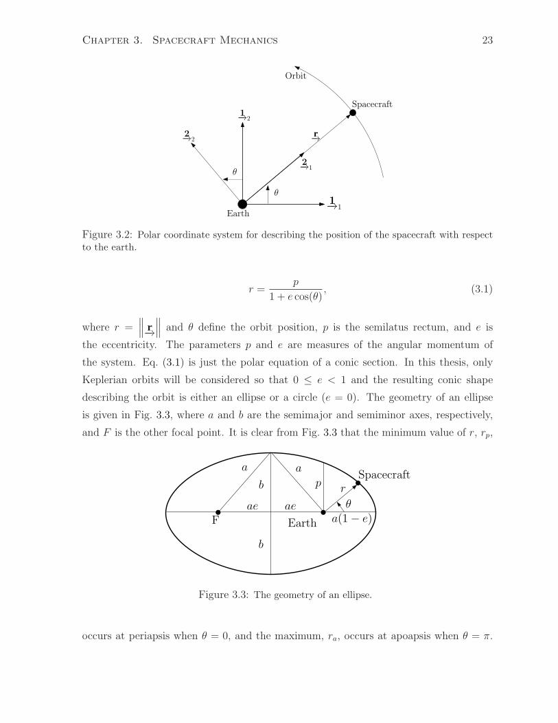
Figure 3.2: Polar coordinate system for describing the position of the spacecraft with respectto the earth.
r =p
1 + e cos(θ), (3.1)
where r =∥∥∥ r−→
∥∥∥ and θ define the orbit position, p is the semilatus rectum, and e is
the eccentricity. The parameters p and e are measures of the angular momentum of
the system. Eq. (3.1) is just the polar equation of a conic section. In this thesis, only
Keplerian orbits will be considered so that 0 ≤ e < 1 and the resulting conic shape
describing the orbit is either an ellipse or a circle (e = 0). The geometry of an ellipse
is given in Fig. 3.3, where a and b are the semimajor and semiminor axes, respectively,
and F is the other focal point. It is clear from Fig. 3.3 that the minimum value of r, rp,
Spacecraft
EarthF
b
b
ae ae θ
a(1− e)
pr
a a
Figure 3.3: The geometry of an ellipse.
occurs at periapsis when θ = 0, and the maximum, ra, occurs at apoapsis when θ = π.

Chapter 3. Spacecraft Mechanics 24
Therefore,
rp =p
1 + e
ra =p
1− e
and a relationship between the semimajor axis and the semilatus rectum can be estab-
lished by noting that
a =rp + ra
2
=p
1− e2. (3.2)
The significance of this relationship is mentioned in Chapter 3.2.2.
3.2.1 Orbit Orientation
The polar coordinate representation of the spacecraft’s orbit (Eq. 3.1) is useful because
it effectively reduces the three-dimensional problem to a planar one. However, the ob-
jective is to describe the position of the spacecraft with respect to the geocentric iner-
tial reference frame F−→i described in Chapter 3.1. Consider an orbital reference frame,
F−→o =[
o−→1
o−→2
o−→3
]T
, that is defined such that o−→1
points in the direction of periapsis,
o−→3
points in the direction of the angular momentum h−→, and whose origin coincides with
F−→i. Then it is clear that o−→1
and o−→2
are the same as 1−→1and 1−→2
in Fig. 3.2. Thus,
the orbit lies on the plane spanned by those two basis vectors and the polar coordinates
can be used. The orientation of the orbit with respect to the inertial frame can then
be described by a rotation matrix, Coi. Fig. 3.4 illustrates the orbital reference frame,
where the angles Ω, i, and ω specify its orientation with respect to F−→i, and n−→ (the line
of nodes) points towards the ascending node (the point where the spacecraft crosses the
equatorial plane from south to north). The parameter Ω ∈ [0, 2π) is called the right
ascension of the ascending node, and it is the angle between i−→1and n−→. The parameter
i ∈ [0, π] is called the inclination and it is the angle from the equatorial plane to the
orbital plane (which is equal to the angle between o−→3
and i−→3). The third parameter,
ω ∈ [0, 2π), is called the argument of periapsis and it is the angle between the line of
nodes ( n−→) and the periapsis direction ( o−→1
). These parameters are chosen such that they
form a 313-Euler angle, whose rotation matrix, Coi is easily obtained (see Chapter 2.2.1

Chapter 3. Spacecraft Mechanics 25
i−→3
Spacecraft
Earth
i−→1
, à
n−→
i−→2
o−→1
Periapsis Directionr−→
h−→
, o−→3
Equator
i
θ
ω
Ω
Figure 3.4: The orbital and inertial reference frames.
for a description of Euler angles) and is given by
Coi = C3(ω)C1(i)C3(Ω)
=
cΩcω − sωcisΩ sΩcω + cisωcΩ sisω
−cΩsω − cωcisΩ −sΩsω + cωcicΩ sicω
sΩsi −sicΩ ci
. (3.3)
Once the orbital position of the spacecraft is known in F−→o, the inertial position can be
obtained by multiplying it by Cio = C−1oi = CT
oi (where the equalities follow from the
orthogonality of a rotation matrix).
3.2.2 Orbital Elements
It is clear that the parameters a and e fully specify the size and shape of the elliptical
orbit. The parameters Ω, i, and ω specify the orientation and location of the orbit with
respect to inertial space. One last parameter needs to be defined in order to temporally
locate an initial reference position of the spacecraft within the orbit. The time of periapsis
passage, t0 is typically used.
The six parameters a, e, t0, Ω, i, and ω are called the classical orbital elements and
together they are able to fully specify the position ( r−→) and velocity ( r−→) of the spacecraft
Chapter 3. Spacecraft Mechanics 26
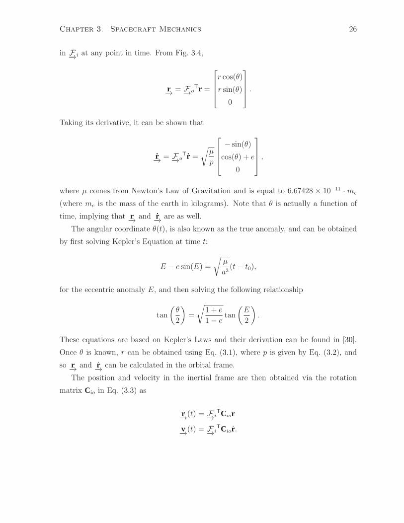
in F−→i at any point in time. From Fig. 3.4,
r−→ = F−→oTr =
r cos(θ)
r sin(θ)
0
.
Taking its derivative, it can be shown that
r−→ = F−→oTr =
õ
p
− sin(θ)
cos(θ) + e
0
,
where µ comes from Newton’s Law of Gravitation and is equal to 6.67428 × 10⁻¹¹ ·me
(where me is the mass of the earth in kilograms). Note that θ is actually a function of
time, implying that r−→ and r−→ are as well.
The angular coordinate θ(t), is also known as the true anomaly, and can be obtained
by first solving Kepler’s Equation at time t:
E − e sin(E) =
õ
a3(t− t0),
for the eccentric anomaly E, and then solving the following relationship
tan
(θ
2
)
=
√
1 + e
1− etan
(E
2
)
.
These equations are based on Kepler’s Laws and their derivation can be found in [30].
Once θ is known, r can be obtained using Eq. (3.1), where p is given by Eq. (3.2), and
so r−→ and r−→ can be calculated in the orbital frame.
The position and velocity in the inertial frame are then obtained via the rotation
matrix Cio in Eq. (3.3) as
r−→(t) = F−→iTCior
v−→(t) = F−→i
TCior .

Chapter 3. Spacecraft Mechanics 27
3.3 Spacecraft Kinematics
An important part of systems control is defining the system’s state variables; that is,
those variables whose motion needs to be controlled. For a spacecraft, the main objec-
tive tends to include being able to point it in a certain direction. In this case, the state
variables desiring control would be parameters describing its orientation (i.e., quater-
nions). Spacecraft kinematics deals with the rate of change of the spacecraft’s attitude
as it orbits around the earth. The orientation of the spacecraft will be characterized
using the quaternion parameterization of the rotation matrix Cbi as described in Chap-
ter 2.2.2. In the following discussions, all variables without a subscript will be taken
to be expressed in the body-fixed frame F−→b. The subscript ‘i’ will be used to denote
variables in the geocentric inertial frame F−→i.
To obtain the kinematic equations of motion, a relationship between the angular
velocity ω−→bi= F−→b
Tω and the inertial time derivative of the rotation matrix is needed.
The two frames can be related to each other by noting that
F−→iT = F−→b
TCbi.
Taking the inertial time derivative one obtains
F−→iT
= F−→bT
Cbi + F−→bTCbi
0−→ = ω−→× F−→bTCbi + F−→b
TCbi
0−→ = ωTF−→b × F−→bTCbi + F−→b
TCbi
0−→ = F−→bT
(
ω×Cbi + Cbi
)
,
which implies that
ω× = −CbiCbi. (3.4)
Substituting Eq. (2.1) into Eq. (3.4) one obtains
ω× = φa× − (1− cos(φ))(a×a
)×
+ sin(φ)a×,
and it follows that
ω = φa− (1− cos(φ))a×a+ sin(φ)a.
Chapter 3. Spacecraft Mechanics 28
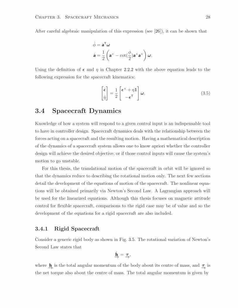
After careful algebraic manipulation of this expression (see [26]), it can be shown that
φ = aTω
a =1
2
(
a× − cot(φ
2)a×a×
)
ω.
Using the definition of ǫ and η in Chapter 2.2.2 with the above equation leads to the
following expression for the spacecraft kinematics:
[
ǫ
η
]
=1
2
[
ǫ× + η1
−ǫT
]
ω. (3.5)
3.4 Spacecraft Dynamics
Knowledge of how a system will respond to a given control input is an indispensable tool
to have in controller design. Spacecraft dynamics deals with the relationship between the
forces acting on a spacecraft and the resulting motion. Having a mathematical description
of the dynamics of a spacecraft system allows one to know apriori whether the controller
design will achieve the desired objective, or if those control inputs will cause the system’s
motion to go unstable.
For this thesis, the translational motion of the spacecraft in orbit will be ignored so
that the dynamics reduce to describing the rotational motion only. The next few sections
detail the development of the equations of motion of the spacecraft. The nonlinear equa-
tions will be obtained primarily via Newton’s Second Law. A Lagrangian approach will
be used for the linearized equations. Although this thesis focuses on magnetic attitude
control for flexible spacecraft, comparisons to the rigid case may be of value and so the
development of the equations for a rigid spacecraft are also included.
3.4.1 Rigid Spacecraft
Consider a generic rigid body as shown in Fig. 3.5. The rotational variation of Newton’s
Second Law states that
h−→ = τ−→,
where h−→ is the total angular momentum of the body about its centre of mass, and τ−→ is
the net torque also about the centre of mass. The total angular momentum is given by

Chapter 3. Spacecraft Mechanics 29
F−→b
dm
ρ−→
b−→1
b−→2
b−→3
V
Figure 3.5: A generic rigid body.
h−→ =
∫
V
ρ−→
× ρ−→dm,
and its inertial time derivative is then
h−→ =
∫
V
ρ−→
× ρ−→
+ ρ−→
× ρ−→dm
=
∫
V
ρ−→
× ρ−→dm, (3.6)
since the cross product of a vector and itself is zero. The acceleration ρ−→
can be found
by noting that
ρ−→= 0−→ (by the rigid assumption) and so
ρ−→
=
ρ−→
+ω−→bi× ρ
−→
ρ−→
= ω−→bi× ρ
−→
ρ−→
= ω−→bi×
ρ−→
+
ω−→bi× ρ−→
+ ω−→bi×(
ω−→bi× ρ
−→
)
ρ−→
=
ω−→bi× ρ−→
+ ω−→bi×(
ω−→bi× ρ−→
)
.
Eq. (3.6) then becomes
h−→ =
∫
V
ρ−→
×(
ω−→bi× ρ−→
)
+ ρ−→
×(
ω−→bi×(
ω−→bi× ρ−→
))
dm
=
∫
V
− ρ−→
(
× ρ−→×
ω−→bi
)
dm+
∫
V
ρ−→
×(
ω−→bi×(
ω−→bi× ρ−→
))
dm,

Chapter 3. Spacecraft Mechanics 30
where the second term in the above equation can be written as
ρ−→
×(
ω−→bi×(
ω−→bi× ρ−→
))
= − ρ−→
×(
ω−→bi×(
ρ−→
× ω−→bi
))
= ρ−→
×(
ρ−→
× ω−→bi
)
× ω−→
= −ω−→bi×(
ρ−→
×(
ρ−→
× ω−→bi
))
.
Expressing everything in F−→b, and noting that ω−→bi= F−→b
Tω is independent of the variable
of integration leads to the following equation:
h =
∫
V
(−ρ×ρ×
)dm ω + ω×
∫
V
(−ρ×ρ×
)dm ω.
It can be shown by direct expansion that the term∫
V(−ρ×ρ×) dm = I , where I is the
body’s mass moment of inertia. The dynamics of a rigid spacecraft, expressed in the
body frame, are then given by
I ω + ω×Iω = τ , (3.7)
which is just a statement of Euler’s Equation for rigid-body dynamics. Eqs. (3.5)
and (3.7) fully specify the motion of a rigid spacecraft.
3.4.2 Flexible Spacecraft
The equations of motion for a flexible spacecraft are obtained in a similary manner as
in Chapter 3.4.1. Consider a generic unconstrained flexible body where the undeformed
position of a mass element dm and its deformation are denoted in the body frame by ρ and
ue(ρ, t) respectively, as seen in Fig. 3.6. Assuming a Ritz expansion for the deformation
field, the deformation at a given point on the body can be described in F−→b as
ue(ρ, t) =N∑
i=1
ψi(ρ)qei(t), (3.8)
where qei are the generalized deformation degrees of freedom; and ψi are basis functions
that describe the deformation field while satisfying the following boundary conditions:
ψi(0) = 0
∇×ψi(0) = 0.

Chapter 3. Spacecraft Mechanics 31
F−→b dm
ρ−→
u−→e
r−→
b−→3
b−→1
b−→2
Figure 3.6: A generic unconstrained flexible body.
The total acceleration of a differential mass element, r−→, as expressed in F−→b, can be
derived using a similar process as in Chapter 3.4.1:
r−→ = F−→bT (ρ+ ue)
r−→ = F−→bT(ω×ρ+ ue + ω
×ue
)
r−→ = F−→bT(ω×ω×ρ+ ω×ρ+ ue + 2ω×ue + ω
×ω×ue + ω×ue
).
Using Newton’s second law, summing over the entire body, and premultiplying the ac-
celeration by a moment arm it is clear that
∫
V
ρ−→
× r−→ dm = τ−→,
where τ−→ is then the net torque. Expanding this expression and using the Ritz approx-
imation for ue, the net torque acting on the spacecraft is governed (as seen in the body
frame) by
τ = I ω +
[N∑
i=1
∫
V
−ρ×ψ×
i dm qei
]
ω + ω×Iω
+ ω×
[N∑
i=1
∫
V
−ρ×ψ×
i dm qei
]
ω + 2
[N∑
i=1
∫
V
−ρ×ψ×
i dm qei
]
ω
+
[N∑
i=1
∫
V
ρ×ψidm qei
]
, (3.9)

Chapter 3. Spacecraft Mechanics 32
where once again I =∫
V−ρ×ρ×dm is the total mass moment of inertia of the body.
Similarily, if the shape functions are projected onto r−→ (which is equivalent to the force
per unit mass) one obtains ∫
V
ψT
i a dm = fe,
where a is the components of r−→ as expressed in F−→b, and fe =[
fe1 · · · feN
]T
is the force
per unit mass projected onto the shape functions. After expanding as above and adding
the contribution to fe due to the structural and damping forces one obtains
fei = ωT
[∫
V
ρ×ψ×
i dm
]
ω +
[∫
V
−ψT
i ρ×dm
]
ω +N∑
j=1
∫
V
ψT
i ψjdm qej
+ 2
[N∑
j=1
∫
V
−ψT
i ψ×
j dm qej
]
ω + ωT
[N∑
j=1
∫
V
ψ×
i ψ×
j dm qej
]
ω
+
[N∑
j=1
∫
V
−ψT
i ψ×
j dm qej
]
ω +N∑
j=1
(K ee)ij qej +N∑
j=1
(Dee)ij qej. (3.10)
The external forces fei are equal to zero for this particular system, since there is phys-
ically no actuator on the spacecraft to provide it. The stiffness term, K ee, comes from
including the resultant force on the system due to the deformation of the flexible body
(see Chapter 3.4.3). Chapter 3.4.4 shows how the damping term, Dee, is obtained. Com-
bined, Eqs. (3.9) and (3.10) represent the complete nonlinear attitude dynamics of the
flexible spacecraft, as expressed in the body frame.
3.4.3 Linearized Equations of Motion
Although the spacecraft dynamics are nonlinear, it is often the case where the system’s
state variables are small enough that the dynamics can be effectively approximated as
linear. A simple rate feedback such as B-control can be used to slow the spacecraft’s
motion down enough so it may be approximated by a linear system [28]. The complexity
of designing and proving the stability of a controller can be significantly reduced when
dealing with a linear system. Also, Lyapunov’s Indirect Method (see Chapter 2.5.2) states
that if the linearized system is asymptotically stable in the sense of Lyapunov, then so
is the nonlinear system (although not necessarily globally) [28]. Designing a controller
based on the linearized system can therefore be advantageous. Thus, a description of
the linearized spacecraft dynamics may be useful. A Lagrangian approach will be used

Chapter 3. Spacecraft Mechanics 33
to obtain the linearized equations of motion. Without loss of generality, the nonlinear
system will be linearized about the operating point/equilibrium ǫ = 0, η = 1, ω = 0,
and qe = 0.
For the rigid spacecraft, it is noted that the source of nonlinearity is due to the second
term on the left-hand side of Eq. (3.7). Parameterizing the spacecraft attitude using an
Euler sequence (described in Chapter 2.2.1), the angular velocity, ω, is related to the
Euler angles, θ, via the relation
ω = S(θ)θ,
where the matrix S depends on the Euler sequence chosen; for a 321-Euler sequence it is
given by
S(θ) =
1 0 − sin(θ2)
0 cos(θ1) sin(θ1) cos(θ2)
0 − sin(θ1) cos(θ1) cos(θ2)
.
It is clear that for small angles (θi << 1) S ≈ 1, where 1 is the identity matrix, and so
ω ≈ θ. Substituting this into Eq. (3.7) and assuming that the angular rates are small as
well (θi << 1), the second-order terms become very small and can be neglected leading
to the heavily linearized equations of motion for the rigid spacecraft given by
I θ = τ . (3.11)
In terms of the kinematic equations of motion, for small angles θ ≈ 2ǫ.
To obtain the linear equations of motion for the flexible spacecraft Lagrange’s equa-
tions will be used. Recalling Fig. 3.6, the velocity of a differential mass element, r−→ =
F−→bTv, is given in the body frame by
v = −ρ×ω + ue + ω×ue.
Assuming that the elastic deflections and angular rates are small, it is defensable to
neglect the last term in the above equation.

Chapter 3. Spacecraft Mechanics 34
The total kinetic energy, T , of the system is given by
T =1
2
∫
V
vTv dm
=1
2
∫
V
(−ρ×ω + ue
)T (−ρ×ω + ue
)dm
=1
2
∫
V
(−ρ×ω
)T (−ρ×ω
)+(−ρ×ω
)Tue + uT
e
(−ρ×ω
)+ uT
e ue dm
=1
2
∫
V
ωT(−ρ×ρ×
)ω
︸ ︷︷ ︸
a
+2ωTρ×ue︸ ︷︷ ︸
b
+ uT
e ue︸︷︷︸
c
dm.
Making the same small angle approximation as for the rigid case, ω ≈ θ, and using the
Ritz expansion for ue the terms a, b, and c in the kinetic energy integral can be written
as
a = ωT(−ρ×ρ×
)ω b = ωTρ×ue c = uT
e ue
= θT(−ρ×ρ×
)θ, = θT
(N∑
i
ρ×ψiqei
)
=
(N∑
i
ψT
i qei
)(N∑
j
ψj qej
)
= θT[
ρ×ψ1 · · · ρ×ψN
]
qe = qT
e
ψT
1ψ1 · · · ψT
1ψN
.... . .
...
ψT
Nψ1 · · · ψT
NψN
qe,
= qT
e
[
ρ×ψ1 · · · ρ×ψN
]T
θ,
where qe =[
qe1 · · · qeN
]T
, and N is the number of flexible degrees of freedom used in
the Ritz expansion. Letting
q =[
θT qT
e
]T
,
M rr = I =∫
V
−ρ×ρ× dm,
M re =
∫
V
[
ρ×ψ1 · · · ρ×ψN
]
dm, and
M ee =
∫
V
ψT
1ψ1 · · · ψT
1ψN
.... . .
...
ψT
Nψ1 · · · ψT
NψN
dm

Chapter 3. Spacecraft Mechanics 35
the kinetic energy can be written as
T =1
2qTMq,
where
M = MT =
[
M rr M re
MT
re M ee
]
.
It is important to note that M > 0 (meaning that it is positive definite).
The potential energy, U , is just the strain energy of the elastic body and is given by
U =1
2
∫
V
εTEε dV,
where ε (ue) and E are the strain tensor and elastic modulus, respectively. The strain
tensor can be written as
ε(ue) = ε
(N∑
i=1
ψiqei
)
=N∑
i=1
ε (ψi) qei.
The potential energy then becomes
U =1
2
N∑
i=1
N∑
j=1
∫
V
ε (ψi)T Eε (ψi) dV qeiqej
=1
2qTKq ,
where
K = KT =
[
0 0
0 K ee
]
and
[K ee]ij =
∫
V
εT (ψei)Eε (ψej) dV.
Given the form of K , it is clear that K ≥ 0 (meaning it is positive semidefinite).
By examining the virtual work done by a force f−→e= F−→b
Tfe causing a virtual dis-
placement of the mass element dm, it can shown that the resulting generalized force fw

Chapter 3. Spacecraft Mechanics 36
acting on the system is given by
fw =
[
g
fe
]
,
where g =∫
Vρ×fe dV = τ is the total torque acting on the spacecraft body, and
fei =∫
VψT
i fe dV is the total force projected onto the flexible degrees of freedom (which
is equal to zero for this particular system).
It is assumed that in any real system the flexible degrees of freedom have some
damping associated with them. This damping is added to the system in the form of a
generalized force f−→d= F−→b
Tfd, given by
fd = −Dq,
where
D = DT =
[
0 0
0 Dee
]
,
and Dee is obtained as in Chapter 3.4.4 so as to ensure that only the flexible modes are
being damped. Given the form of D, it is clear that D ≥ 0 as well.
Applying Lagrange’s equations, which are given by
d
dt
(∂L
∂qi
)
−∂L
∂qi= fi,
where L = T − U and f = fw + fd, the linearized equations of motion for the flexible
spacecraft can be written as
Mq + Dq + Kq = fw, (3.12)
where for this thesis fw =[
τT 0T
]T
. The linearized equations could also have been
obtained by letting ω = θ in Eqs. (3.9) and (3.10) and taking the Jacobian around the
operating point θ = θ = qe = qe = 0.
3.4.4 Modal Equations of Motion
Decomposing Eq. (3.12) into modal coordinates allows the dynamics of the system to
be evaluated in terms of its fundamental modes of motion. Most importantly, modal
analysis allows for the rigid and flexible motions to be investigated separately, making
it easier to assess the contribution of the flexibility of the spacecraft to the system’s

Chapter 3. Spacecraft Mechanics 37
dynamics.
Consider the unforced version of Eq. (3.12), which is given by
Mq + Kq = 0. (3.13)
Note that the effect of damping can be considered as an external force acting on the
system. It is assumed that an arbitrary solution to the above equation can be written as
q(t) = qαeλαt,
where the subscript α refers to a particular degree of freedom. Substituting this into
Eq. (3.13) gives(λ2αM + K
)qα = 0, (3.14)
which is simply a statement of the eigenproblem for this particular system. For non-trivial
values of qα, the eigenproblem can be solved by finding the roots of the characteristic
equation
det(λ2αM + K
)= 0.
Premultiplying Eq. (3.14) by qHα (where (·)H refers to the conjugate transpose operation)
gives
λ2α = −qHα Kqα
qHα Mqα
.
Since M and K are both symmetric, the numerator and denominator of the above equation
are guaranteed to be real. Furthermore, since M > 0 and K ≥ 0 it follows that λ2α ≤ 0.
From the form of K (as given in Chapter 3.4.3), it is clear that there will be at least three
eigenvalues (λα) equal to zero, corresponding to the the three rigid degrees of freedom
describing a pure rotation of the entire spacecraft about each axis. The other eigenvalues
will be purely imaginary and can be written as
λα = ±jωα,
where ωα can be interpreted as the fundamental frequency of the α’th-mode of vibration.
It is easily shown that the resulting eigencolumns qα are mutually orthogonal with respect

Chapter 3. Spacecraft Mechanics 38
to both the mass and stiffness matrices. If, for nonzero ωα, they are normalized such that
qT
αMqβ = δαβ,
where δαβ refers to the Kronecker delta, then it immediately follows that
qT
αKqβ = ω2αδαβ.
The eigenmatrix containing the eigencolumns for the flexible degrees of freedom can be
written as
Qe = row qαα=1,...,N .
The eigencolumns corresponding to the rigid modes (where ωα = 0) can also be normal-
ized and put into the following matrix form:
Qr =
[
1
0
]
.
Note that Qe ∈ R(3+N)×N , and Qr ∈ R
(3+N)×3. Letting Q =[
Qr Qe
]
, it is clear that
QTMQ =
[
I 0
0 1
]
QTKQ =
[
0 0
0 Ω2
]
,
where
Ω = diag ωα .
The benefit of this eigendecomposition is that it decouples the system dynamics as follows.
The eigencolumns span the entire solution space of the linearized system, and so the
solutions q(t) can be written as
q(t) = Qrηr(t) +N∑
α
qαηα(t)
= Qη(t),
Chapter 3. Spacecraft Mechanics 39
where η(t) =[
ηr(t)T η1(t) · · · ηN(t)
]T
are the modal coordinates. Inserting this
expansion into Eq. (3.12) and premultiplying by QT leads to the following equation:
QTMQ η + QTDQη + QTKQη = QTfw
The mass and stiffness terms are decoupled, and it remains to construct the damping
matrix D such that it too is decoupled and acts only on the flexible degrees of freedom.
Since Eq. (3.12) represents a second order system, the damping coefficients, cα, for the
flexible degrees of freedom will be written as cα = 2ζωα. The damping matrix in modal
coordinates is then given by
Dmodal =
[
0 0
0 2ζΩ
]
.
The damping matrix in physical coordinates (D) is then obtained by
D =(QT)−1
DmodalQ−1.
Letting η =[
ηT
r ηT
e
]T
, where ηr and ηe =[
η1 · · · ηN
]T
denote the rigid and flexible
modes respectively, the above equations reduce to
I ηr = τ (3.15)
ηα + 2ζωαηα + ω2αηα = qT
eαfw α = 1, . . . , N, (3.16)
where fw =[
τT 0T
]T
, and qeα is the α’th column of Qe. Eqs. (3.15) and (3.16) represent
the modal equations of motion.
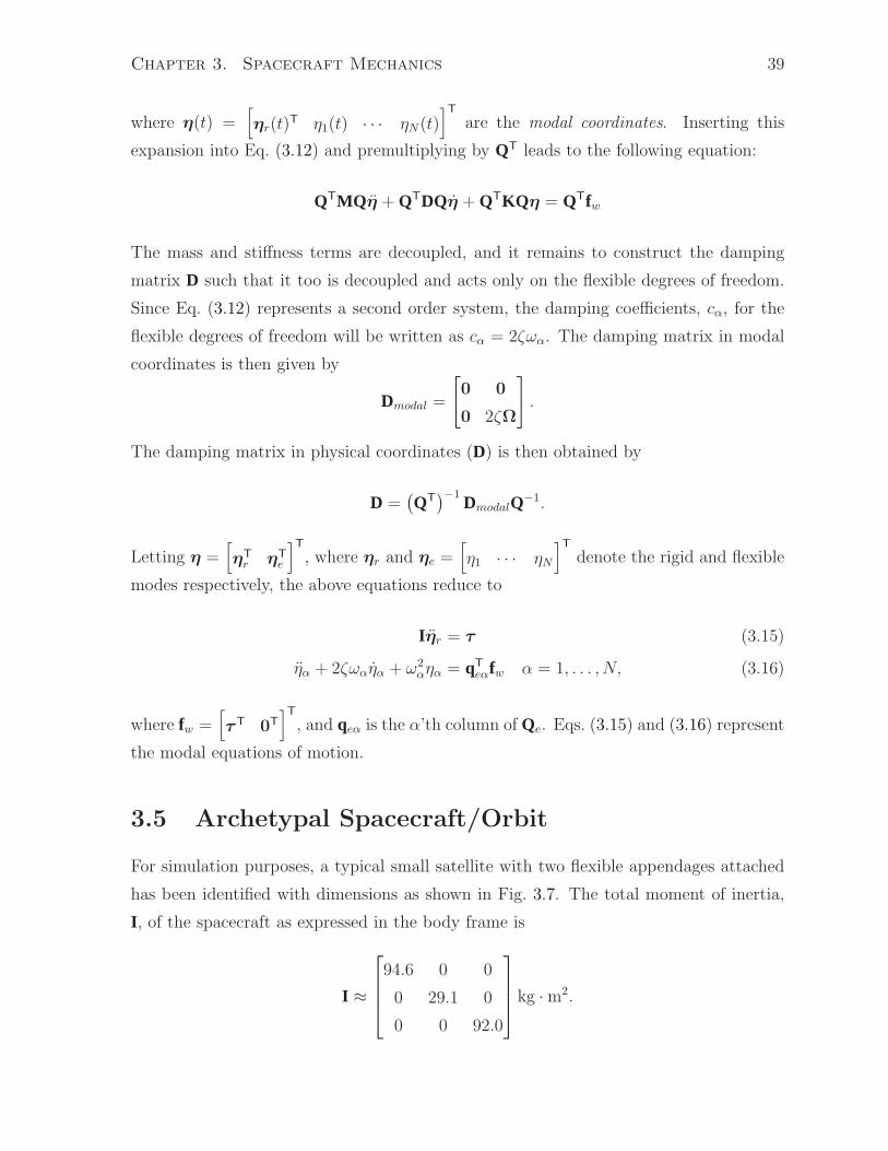
3.5 Archetypal Spacecraft/Orbit
For simulation purposes, a typical small satellite with two flexible appendages attached
has been identified with dimensions as shown in Fig. 3.7. The total moment of inertia,
I , of the spacecraft as expressed in the body frame is
I ≈
94.6 0 0
0 29.1 0
0 0 92.0
kg ·m2.

Chapter 3. Spacecraft Mechanics 40
F−→b
Rigid Body
Flexible Arm
Flexible Arm
0.512 m
1.22 m
1.33 m2 m
0.2 m
0.2 m2 m
0.2 m
0.2 m
M = 106 kg
M = 20 kgM = 20 kg
z
y
x
Figure 3.7: A model rigid spacecraft with two flexible beams attached that will be used foranalysis and simulation purposes.
The appendages will be modeled as uniform cantilevered beams, with Young’s modulus
E = 4×10⁵ Pa and damping ratio ζ = 0.1, and will be allowed to deflect about the body
‘x’ and ‘z’ axes only (i.e., no twisting about the ‘y’ axis). Furthermore, the deflections
about either axis are assumed to be decoupled and small enough such that the spacecraft
moment of inertia remains approximately constant. The shape functions, ψei, needed to
characterize the deformation field of the beam deflections have all been chosen to be of
the form
ψei(y) = cosh(kiy)− cos(kiy) + βi(sin(kiy)− sinh(kiy)),
which represent the exact mode shapes of a cantilevered beam [31]. The first three
modes shapes will be used for each deformation degree of freedom. Table 3.1 contains
the values of βi and ki for the first three modes. The resulting vector shape functions,
Table 3.1: Exact mode shape parameters for cantilevered beam [31].
i βi ki · L1 0.7341 1.87512 1.0185 4.69413 0.9992 7.8548Note: L is the length of the beam.
ψi (in Eq. (3.8)), are then given in a local frame by
ψ1=[
ψe1 0 0]T
ψ2=[
ψe2 0 0]T
ψ3=[
ψe3 0 0]T
ψ4=[
0 0 ψe1
]T
ψ5=[
0 0 ψe2
]T
ψ6=[
0 0 ψe3
]T
,

Chapter 3. Spacecraft Mechanics 41
which describes the deformation field of the flexible arm on the right side of the rigid
body in Fig. 3.7, and
ψ7 =[
−ψe1 0 0]T
ψ8 =[
−ψe2 0 0]T
ψ9 =[
−ψe3 0 0]T
ψ10=[
0 0 ψe1
]T
ψ11=[
0 0 ψe2
]T
ψ12=[
0 0 ψe3
]T
,
which describes the deformation field of the left arm.
A sample orbit is also necessary for simulation purposes. The controllability require-
ments in Chapter 4.2 imply that magnetic attitude control is best suited for orbits that
are low-earth and near-polar. Therefore, the example orbit that will be used in all sim-
ulations (unless otherwise specified) is given by the following orbital elements:
a, e,Ω, i,Ω, t0 = Re+ 450 km, 0, 0, 87, 0, 0 s ,
where Re is the mean radius of the earth. These elements specify a circular orbit with
an inclination of 87 (note that a perfectly polar orbit would have i = 90, see Fig. 3.4).
Chapter 4
Magnetic Attitude Control
As mentioned in Chapter 1, the torque produced via an interaction between a dipole
moment and a magnetic field is given (in the body frame) by
τ = m×b, (4.1)
where τ is the control torque, m is the dipole moment produced by the spacecrafts mag-
netic actuators, and b is the local geomagnetic field vector. In the literature, particularly
for the PD-like control laws, the dipole moment is given by
m = b×ν,
where ν is a new control vector. The resulting expression for the control torque becomes
τ = −b×b×ν. (4.2)
The control torque is expressed in this manner since, for those PD-control laws, the
stability proofs require that
Γ = limT→∞
1
T
∫ T
0
−b×b× dt > 0.
In particular, in [13–16] the positive definiteness of Γ is critical in the Lyapunov stability
proofs. Along with [6], this condition is shown to hold for a dipole approximation of the
geomagnetic field as long as the orbital plane did not coincide with the earth’s equatorial
plane. Since the controller development in Chapter 5 is modelled after the analysis in the
42

Chapter 4. Magnetic Attitude Control 43
references above, Eq. (4.2) will be adopted. A secondary reason for expressing the control
torque as in Eq. (4.2) is that the new control vector ν can be thought of as the actual
resulting torque axis (as it takes into account the cross-product). That is, assuming the
desired torque axis lies on the plane perpendicular to the local geomagnetic field vector,
the axis defined by ν yields a dipole moment such that, after applying Eq. (4.2), τ is
parallel to ν.
4.1 Magnetic Field Model
Since magnetic attitude control relies on the earth’s magnetic field, it is important to
have a suitable magnetic field model, especially for simulation purposes. Although several
models exist, the spherical harmonic model outlined in [1] will be used. This model
assumes that the dominant portion of the earth’s magnetic field, which is denoted by b−→
,
can be described by the gradient of a scalar potential function V . That is, the field can
be described by the relation
b−→
= −∇−→V, (4.3)
where V can be represented by a series of spherical harmonics:
V (r, θ, φ) = a
k∑
n=1
(a
r
)n+1n∑
m=0
(gmn cosmφ+ hmn sinmφ)Pmn (θ) ,
where a is the equatorial radius of the Earth, gmn and hmn are the International Geo-
magnetic Reference Field (IGRF) Gaussian coefficients, Pmn are the Schmidt normalized
Legendre functions, k is the highest spherical harmonic to be considered, and r, θ, and
φ are the geocentric distance, coelevation, and East longitude, which define any point in
space. Note that the above equation only applies if r > a. The gaussian coefficients for
the year 2010 will be used and are given in Table 4.1 (for k = 1, . . . , 5). It is important
to note that the local magnetic field is dependent on the orbital position of the space-
craft, which is a function of time. Therefore, the magnetic field vector experienced by
the spacecraft is implicitly a function of time as well. From Eq. (4.3), the magnetic field

Chapter 4. Magnetic Attitude Control 44
Table 4.1: IGRF Coefficients for Epoch 2010 [32].
n m g (nT) h (nT)1 0 -29496.5 n/a1 1 -1585.9 4945.12 0 -2396.6 n/a2 1 3026.0 -2707.72 2 1668.6 -575.43 0 1339.7 n/a3 1 -2326.3 -160.53 2 1231.7 251.73 3 634.2 -536.84 0 912.6 n/a4 1 809.0 286.44 2 166.6 -211.24 3 -357.1 164.44 4 89.7 -309.25 0 -231.1 n/a5 1 357.2 44.75 2 200.3 188.95 3 -141.2 -118.15 4 -163.1 0.15 5 -7.7 100.9
vector can be expressed as
Br =−∂V
∂r=
k∑
n=1
(a
r
)n+2
(n+ 1)n∑
m=0
(gn,m cos(mφ) + hn,m sin(mφ))P n,m(θ)
Bθ =−1
r
∂V
∂θ= −
k∑
n=1
(a
r
)n+2n∑
m=0
(gn,m cos(mφ) + hn,m sin(mφ))∂P n,m(θ)
∂θ
Bφ =−1
r sin(θ)
∂V
∂φ=
−1
sin(θ)
k∑
n=1
(a
r
)n+2n∑
m=0
m (−gn,m cos(mφ) + hn,m sin(mφ))P n,m(θ),
(4.4)
where gn,m, hn,m, and P n,m(θ) are related to gmn , hmn , and P
mn (θ), respectively (see Ap-
pendix A for their calculation). The reference frame in which Eq. (4.4) holds can be

Chapter 4. Magnetic Attitude Control 45
related to the geocentric inertial frame F−→i (from Chapter 3.1 by noting that
b−→
= F−→iT
(Br cos(δ) +Bθ sin(δ)) cos(α)−Bφ sin(α)
(Br cos(δ) + Bθ sin(δ)) sin(α) + Bφ cos(α)
(Br sin(δ)− Bθ cos(δ))
, (4.5)
where α is the right ascension, and δ = π2− θ is the declination of the spacecraft position
in F−→i. Letting r−→ = F−→iTr = F−→i
T
[
r1 r2 r3
]T
be the position of the spacecraft with
respect to the centre of the earth (as in Fig. 3.1), the right ascension and declination are
given by
α = tan−1
(r2
r1
)
δ = tan−1
(
r3√
r21 + r22
)
.
It is important to note that east longitude φ is related to the right ascension α by
φ = α−
(
αG0 +dαG
dtt
)
,
where αG(t) is the right ascension of the Greenwich meridian and αG0 = αG(0). This
term takes into account the rotation of the earth. Also, the coelevation θ is related to
the declination δ by
θ =π
2− δ.
An important aspect of this model is how the magnetic field observed by a space-
craft as it orbits the earth is approximately periodic. Fig. 4.1 shows the magnetic field
vector expressed in F−→i over a few orbits. The 450 km orbit was taken to have i = 87,
with all other orbital elements equal to zero (see Chapter 3.2.2 for a description of the
orbital elements). The almost periodic nature of the magnetic field means that periodic
controllers (like the ones in [9]) can be developed. It also means that stability theories
that rely on the periodic nature of the system dynamics (such as the Floquet theory in
Chapter 2.4) can be used.

Chapter 4. Magnetic Attitude Control 46
0 0.5 1 1.5 2 2.5 3−5
−4
−3
−2
−1
0
1
2
3
4x 10
−5
# of Orbits
Mag
netic
Fie
ld (
T)
b
1
b2
b3
Figure 4.1: An example of the geomagnetic field experienced by a spacecraft in orbit.
4.2 Controllability
When first attempting to solve the control problem for a given system, it is of interest
to know whether or not the system can actually be controlled (i.e., whether or not there
exists a control vector that is able to take the system from one arbitrary state to a
particular desired state). In the case of magnetic attitude control, the control torque
is goverened by the vector cross-product τ−→ = m−→ × b−→, as mentioned in Chapter 4.
Because of the inherent nature of the cross-product the resulting torque must lie on a
plane perpendicular to the local geomagnetic field vector as seen in Fig. 4.2. This plane
is spanned by two degrees of freedom only, and since the orientation of a spacecraft has
three degrees of freedom in Euclidean space, it is evident that at any point in time, the
spacecraft mechanics are instantaneously underactuated and therefore, uncontrollable.
However, since the spacecraft is orbiting around the earth, the local geomagnetic field
vector that acts on the spacecraft changes with time. It was shown in [6] that under
certain conditions, the mechanics of a spacecraft using magnetic actuation can indeed
be controllable in a time-varying sense. This necessarily makes the control problem a
time-varying one.
The analysis in [6] first develops conditions for accessibility and controllability for
general time-varying systems. Those conditions were then considered for the case of the
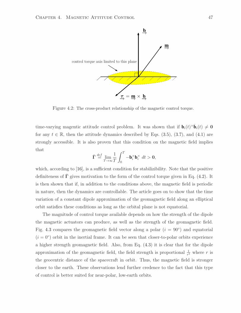
Chapter 4. Magnetic Attitude Control 47
b−→
m−→
τ−→
= m−→
× b−→
control torque axis limited to this plane
Figure 4.2: The cross-product relationship of the magnetic control torque.
time-varying magentic attitude control problem. It was shown that if bi(t)×bi(t) 6= 0
for any t ∈ R, then the attitude dynamics described by Eqs. (3.5), (3.7), and (4.1) are
strongly accessible. It is also proven that this condition on the magnetic field implies
that
Γdef= lim
T→∞
1
T
∫ T
0
−b×
i b×
i dt > 0,
which, according to [16], is a sufficient condition for stabilizibility. Note that the positive
definiteness of Γ gives motivation to the form of the control torque given in Eq. (4.2). It
is then shown that if, in addition to the conditions above, the magnetic field is periodic
in nature, then the dynamics are controllable. The article goes on to show that the time
variation of a constant dipole approximation of the geomagnetic field along an elliptical
orbit satisfies these conditions as long as the orbital plane is not equatorial.
The magnitude of control torque available depends on how the strength of the dipole
the magnetic actuators can produce, as well as the strength of the geomagnetic field.
Fig. 4.3 compares the geomagnetic field vector along a polar (i = 90) and equatorial
(i = 0) orbit in the inertial frame. It can be seen that closer-to-polar orbits experience
a higher strength geomagnetic field. Also, from Eq. (4.3) it is clear that for the dipole
approximation of the geomagnetic field, the field strength is proportional 1r3
where r is
the geocentric distance of the spacecraft in orbit. Thus, the magnetic field is stronger
closer to the earth. These observations lend further credence to the fact that this type
of control is better suited for near-polar, low-earth orbits.

Chapter 4. Magnetic Attitude Control 48
0 0.5 1 1.5 2 2.5 3−1
0
1
2
3x 10
−5
Mag
netic
Fie
ld (
T)
Equatorial Orbit
b
1
b2
b3
0 0.5 1 1.5 2 2.5 3−5
0
5x 10
−5
# of Orbits
Mag
netic
Fie
ld (
T)
Polar Orbit
b
1
b2
b3
Figure 4.3: A comparison of the geomagnetic field for polar and equatorial orbit.
4.3 Hybrid PD-Like Control Law
The controller development for the flexible system (described in Chapter 3) in this thesis
will be based on proportional-derivative (PD) control due to its simplicity, ease of imple-
mentation, and effectiveness. As mentioned in the literature review, several controllers
based on PD-control have been proposed for a rigid spacecraft. Recall that the equations
of motion for the rigid system (see Chapters 3.3 and 3.4.1) are given (in the body frame)
by
[
ǫ
η
]
=1
2
[
ǫ× + η1
−ǫT
]
ω
I ω + ω×Iω = τ . (4.6)

Chapter 4. Magnetic Attitude Control 49
For this rigid system, [13] proposes the following PD-like control law in order to stabilize
the equilibrium ω = 0,[
ǫT η
]T
=[
0 0 0 1]T
:
τ = −b×b×ν
ν = −I−1(ε2kpǫ+ εkdω
). (4.7)
It is important to note that Eq. (4.7) relies on knowledge of the spacecraft inertia matrix
I , potentially making it not robust to model uncertainty. This control law utilizes both
angular velocity and attitude feedback. The stability proof in [13] places an upper bound,
ε∗, on the controller parameter ε, which limits the effectiveness of this type of control.
This bound is also shown to exist for the similar PD-like controllers proposed in [14–16].
In [13], the closed-loop equations of motion are re-cast (after a coordinate transformation)
into the form
x = εf(x, ε),
and the generalized averaging theory described in [17] is applied, which states that for
ε < ε∗ the trajectories of a non-autonomous system remain close to the trajectories of
the averaged system. The non-autonomous part of Eq. (4.7) is the term −b×b×, and it
is replaced by its average (similar to Γ in Chapter 4.2). The averaged equations then
describe an LTI system, and stability for the averaged system is proven via Lyapunov’s
Direct Method. The existence of ε∗ can be reasoned as ensuring that the response of the
system (determined by x) is much slower than the excitation (given by f), making the
response predominantly determined by the average of the excitation. A more physical
approach can also be taken to explain the existence of ε∗. Consider the energy E of the
linearized version of the above control system, given by
E =1
2θTI θ +
1
2θTKθ,
where K = −ε2kpI−1b×b×I−1. Its time rate of change is given by
E =1
2θTKθ − θTDθ,
where D = −εkdI−1b×b×I−1 ≥ 0. It is clear that since the first term is indefinite, and
the second term is negative semi-definite, the controller parameters must be carefully
chosen such that the rate of change of the energy is not increasing in order to have any

Chapter 4. Magnetic Attitude Control 50
chance for stability. This requirement manifests itself as a bound on ε. It should be
noted that without the attitude feedback, K = 0 and E ≤ 0 is satisfied for any choice of
ε. Thus, it is evident that ε∗ places restrictions on the ratio of proportional to derivative
control. Fig. 4.4 demonstrates the existence of ε∗ for the controller given by Eq. (4.7),
on the nonlinear rigid system described in Chapter 3. The plots on the left show the
trajectories of the system when ε = 0.001, and those on the right show when ε = 0.003,
with initial conditions of ω =[
0.05 0.05 0.05]T
and all else zero.
0 1 2 3−1
0
1
2ε = 0.001
Qua
tern
ions
ǫ1ǫ2ǫ3η
0 1 2 3−0.05
0
0.05
0.1
0.15
# of Orbits
Ang
ular
Vel
ocity
(ra
d/s)
ω1
ω2
ω3
0 1 2 3−1
0
1
2ε = 0.003
ǫ1ǫ2ǫ3η
0 1 2 3−0.05
0
0.05
0.1
0.15
# of Orbits
ω1
ω2
ω3
Figure 4.4: Plots of the trajectories of a system using the control law in Eq. (4.7), demonstrat-ing the existence of ε∗.
In [24], it is shown that the limitation on the control gains under purely magnetic
actuation (for the system shown above) can be removed with the addition of a mini-
mum level of alternate, independent three-axis actuation (i.e., using thrusters or reaction
wheels). In order to stabilize the same equilbirium as above, [24] proposes the following
control law:
τ = −‖bi‖−2 b×b×ν + u,

Chapter 4. Magnetic Attitude Control 51
where
ν = −I−1(2ε2kpǫ+ εkdω
)
is the control effort given by the magnetic actuators and
u = −γI−1(2ε2kpǫ+ εkdω
)
is that given by the alternate three-axis actuation system. The law for the control
vector u includes the parameter ε so that the new control parameter γ can be seen as a
dimensionless scaling that is a kind of measure of the amount of torque provided by the
three-axis actuation over that provided by the magnetic actuators. It is shown in [24]
that if γ >kpλ2
max
k2d
, with ε, kp, and kd all greater than zero, and where λmax is the
largest principal moment of inertia, then the system is asymptotically stable. Thus, with
minimum control effort provided by the alternate three-axis actuator, the system can be
guaranteed to be stable, even for ε > ε∗. The controller design in the following chapter
will attempt to extend the work done in [24] to the flexible spacecraft case.

Chapter 5
Hybrid PD-Control Of Flexible
Spacecraft
Without loss of generality, the control problem is defined to be the stabilization of the
equilibrium ω = 0,[
ǫT η
]T
=[
0 0 0 1]T
. The controller design in this section is
based on the PD-like control methods discussed in Chapter 4.3. It is important to note
that [25] proposes a PD-like control law in order to stabilize the flexible system using
magnetic actuation. The control law takes the form
τ = −‖bi‖−2 b×b×ν,
where
ν = −(ε2kpI−1ǫ+ εkdIω
).
As with the other laws that contained attitude feedback, limitations are placed on the
size of the control gains. Also, since the moment of inertia appears in the control law, it
lacks robustness against model uncertainty. A more robust version that eliminates the
controller’s dependency on the spacecraft inertia can be found (for the rigid case) in [15].
It will serve as the starting point of the controller design for the flexible case.
The nonlinear equations of motion for the flexible system (see Chapter 3) are very
complex to work with, and so the controller development will focus on the linearized
system. After stabilizing the linear system, Lyapunov’s Indirect Method can then be
applied to draw conclusions for the nonlinear case. Also, working with the linearized sys-
tem allows for the application of Floquet analysis, which is a useful tool for investigating
the control gain stability criteria.
52

Chapter 5. Hybrid PD-Control Of Flexible Spacecraft 53
Recall the linearized equations of motion for the flexible spacecraft, which are given
by
Mq + Dq + Kq = fw, (5.1)
where fw =[
τT 0T
]T
(see Chapter 3.4.3 for the definitions of the other variables in
Eq. (5.1)). It is assumed that the spacecraft orbit is such that
Γi = limT→∞
1
T
∫ T
0
Γi dt > 0,
where
Γidef= −‖bi‖
−2 b×
i b×
i ≥ 0.
It is shown in [25] that for sufficiently small angular velocities, if the above holds true
then it also holds when bi is replaced with b, the magnetic field vector in the body frame,
meaning that
Γ = limT→∞
1
T
∫ T
0
Γ dt > 0,
where
Γdef= −‖bi‖
−2 b×b× ≥ 0.
Note that this requirement was shown in [6] to be true for the dipole approximation of
the geomagnetic sphere, as long as the orbital plane was not equatorial. Also, b = Cbibi
which for small angles Cbi = 1 − θ×. With the linear assumption, the −θ× term leads
to products of small angles and rates, meaning that b can, and will, be approximated by
bi.
Consider the purely magnetic control law given by
τ = Γν
ν = −(2ε2kpǫ+ εkdω
),
which, after linearizing (i.e., letting θ ≈ 2ǫ, θ ≈ ω) becomes
τ = −Γ(
ε2kpθ + εkdθ)
= −Γc(ε2kpq + εkdq
), (5.2)
where c =[
1 0T
]
, and q =[
θT qT
e
]T
. Substituting the above into Eq. (5.1), the
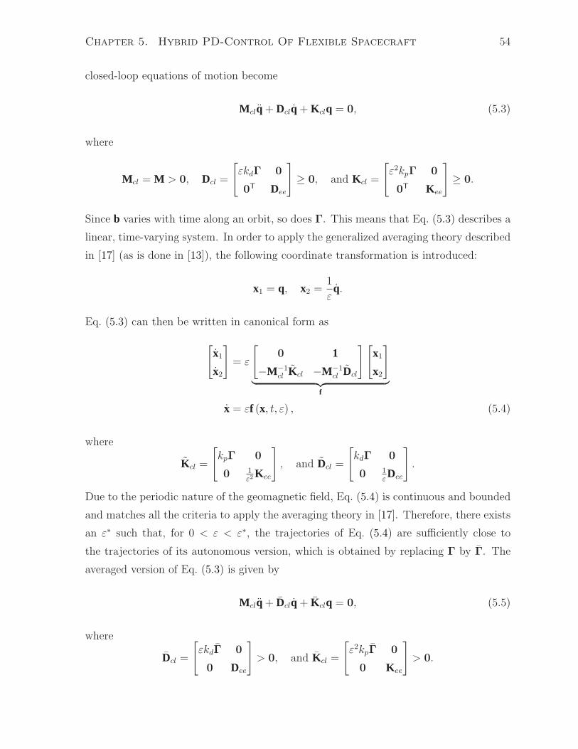
Chapter 5. Hybrid PD-Control Of Flexible Spacecraft 54
closed-loop equations of motion become
M clq + Dclq + K clq = 0, (5.3)
where
M cl = M > 0, Dcl =
[
εkdΓ 0
0T Dee
]
≥ 0, and K cl =
[
ε2kpΓ 0
0T K ee
]
≥ 0.
Since b varies with time along an orbit, so does Γ. This means that Eq. (5.3) describes a
linear, time-varying system. In order to apply the generalized averaging theory described
in [17] (as is done in [13]), the following coordinate transformation is introduced:
x1 = q, x2 =1
εq.
Eq. (5.3) can then be written in canonical form as
[
x1
x2
]
= ε
[
0 1
−M−1cl K cl −M−1
cl Dcl
][
x1
x2
]
︸ ︷︷ ︸
f
x = εf (x, t, ε) , (5.4)
where
K cl =
[
kpΓ 0
0 1ε2
K ee
]
, and Dcl =
[
kdΓ 0
0 1εDee
]
.
Due to the periodic nature of the geomagnetic field, Eq. (5.4) is continuous and bounded
and matches all the criteria to apply the averaging theory in [17]. Therefore, there exists
an ε∗ such that, for 0 < ε < ε∗, the trajectories of Eq. (5.4) are sufficiently close to
the trajectories of its autonomous version, which is obtained by replacing Γ by Γ. The
averaged version of Eq. (5.3) is given by
M clq + Dclq + K clq = 0, (5.5)
where
Dcl =
[
εkdΓ 0
0 Dee
]
> 0, and K cl =
[
ε2kpΓ 0
0 K ee
]
> 0.

Chapter 5. Hybrid PD-Control Of Flexible Spacecraft 55
The positive semidefiniteness of Dcl and K cl where due to the fact that Γ ≥ 0. However,
since Γ > 0, Dcl and K cl are positive definite as well.
The stability of the averaged system can be shown via Lyapunov’s Direct Method.
Consider the candidate Lyapunov function given by
V =1
2qTM clq + qTK clq > 0.
The function V is clearly positive definite and furthermore, it is radially unbounded. Its
derivative is given by
V = −qTDclq ≤ 0.
Although V is negative semidefinite with respect to the system state[
qT qT
]T
, it is
evident that q = 0 ⇒ q = 0 ⇒ K clq = 0 ⇒ q = 0 and so LaSalle’s theorem can be
applied. Therefore, the averaged, autonomous, closed-loop system described by Eq. (5.5)
is asymptotically stable. This implies that for ε < ε∗, the non-autonomous, closed-loop
system given by Eq. (5.3) is also asymptotically stable about the equilibrium q = q = 0,
since its trajectories remain close to those of the autonomous system.
As is done in [24], an independent control vector u will be added representing the
torque caused by an alternate three-axis actuator such as reaction wheels or thrusters.
The purpose of adding another control actuator is to alleviate the gain restriction of
purely magnetic attitude control. The control vector fw (from Eq. (5.1)) can then be
written as
fw =
[
τ + u
0
]
,
where τ is the magnetic control given by Eq. (5.2), and
u = −γ(2ε2kpǫ+ εkdω
).
In this control law, ε is included so that the additional control parameter γ acts as a
dimensionless scaling of the amount of non-magnetic control. This further emphasizes
the fact that u is meant to augment the magnetic control; it is not the primary method
of actuation. After linearizing and manipulation, the final hybrid control law is given by
fw = −B(ε2kpq + εkdq
), (5.6)

Chapter 5. Hybrid PD-Control Of Flexible Spacecraft 56
where
B =
[
(γ1+ Γ) 0
0 0
]
.
It should be noted that for purely non-magnetic control (i.e., τ = 0), the closed-loop
equations of motion would be autonomous, and the stiffness and damping matrices would
be positive definite. Asymptotic stability could be shown by choosing a Lyapunov func-
tion identical to V above. The following sections investigate the gain criteria achieving
stability with a minimum contribution from u (measured by the control parameter γ).
5.1 Floquet Stability Analysis
The Floquet theory described in Chapter 2.4 was applied to the baseline sample spacecraft
outlined in Chapter 3.5. Since Floquet theory is a linear analysis, the linearized equations
of motion were used. The dynamics are summarized by
Mq + Dq + Kq = fw,
where fw represents the hybrid control law given as
fw = −B(ε2kpq + εkdq
).
From the equations above, the system matrix A(t) corresponding to the one in Eq. 2.4
in Chapter 2.4 can be written as
A(t) =
[
0 1
−M−1 (K + ε2kpB) −M−1 (D + εkdB)
]
,
with the system state variable being x =[
qT qT
]T
. The Floquet stability analysis was
used to investigate the values of ε and γ that would yield a stable system. For each
ε and γ pair, the theory was applied and the stability of the system was investigated.
Fig. 5.1 represents a stability matrix illustrating the results of the analysis. The control
parameter ε was varied from 0.0001 to 0.02, and γ was varied from 0 to 0.0035 (both
using a uniformally spaced mesh). Note that kp = 25000 kg·m2
s2and kd = 25000 kg·m2
sfor
all graphs unless otherwise specified. In the diagram, a “∗” signifies that the system was
found to be asymptotically stable whereas a “” denotes an unstable system.

Chapter 5. Hybrid PD-Control Of Flexible Spacecraft 57
0 0.5 1 1.5 2 2.5 3 3.5
x 10−3
0.002
0.004
0.006
0.008
0.01
0.012
0.014
0.016
0.018
γ
ε
Figure 5.1: Stability diagram obtained using Floquet theory for the baseline sample spacecraft(∗ = L-stable, = unstable).
Fig. 5.1 clearly confirms the existence of an ε∗ since when looking at the vertical
axis (γ = 0), it is evident that above a certain value of ε the system goes unstable and
remains unstable. Based on the diagram ε∗ ≈ 0.0006853 but if a finer mesh is adopted,
Floquet theory predicted that ε∗ ≈ 0.0002. In general, Fig. 5.1 shows that as ε increases,
less control effort from the non-magnetic actuation system is needed. Typically with the
PD control of LTI systems, larger gains equates to better performance. Fig. 5.2 shows a
comparison of the simulated response of the spacecraft under purely magnetic actuation
for ε = 0.0001 and ε = 0.0002, with an initial condition of θ =[
0.001 0.001 0.001]T
rads
(all else zero). It is clear that for ε = 0.0002 the spacecraft motion eventually goes
unstable, and the system’s states start to grow without bound. Note that for each of the
simulations the stability of the flexible degrees of freedom (qe) matched that of the rigid
degrees of freedom and are omitted from the plot.
An interesting aspect of Fig. 5.1 is the region roughly spanned by 0 < γ < 0.0002
and 0.012 < ε < 0.017. This region is plotted in Fig. 5.3. It can be seen that there is
a curious spur in the stability map where, as γ is increased, the system’s stability goes

Chapter 5. Hybrid PD-Control Of Flexible Spacecraft 58
0 5 10 15−1
−0.5
0
0.5ǫ = 0.0001
Eul
er A
ngle
s (r
ad)
θ1
θ2
θ3
0 5 10 15−1
−0.5
0
0.5
1x 10
−3
# of Orbits
Ang
ular
Vel
ocity
(ra
d/s)
θ1
θ2
θ3
0 5 10 15−4000
−2000
0
2000ǫ = 0.0002
Eul
er A
ngle
s (r
ad)
θ1
θ2
θ3
0 5 10 15−2
0
2
4
# of Orbits
Ang
ular
Vel
ocity
(ra
d/s)
θ1
θ2
θ3
Figure 5.2: Simulated spacecraft motion for ε = 0.0001 and ε = 0.0002, demonstrating thegain limitations when using purely magnetic control.
from unstable to stable to unstable to stable. Causes for this curiosity are not quite
clear. Simulating the system at the boundaries of the spur confirmed the results of the
Floquet analysis, suggesting that it is not merely an artifact of the stability theory. A
similar spur was found to exist in [33], where the stability properties (using the hybrid
control law in [24]) of a spacecraft with different inertia properties was investigated.
The stability maps for the equivalent rigid spacecraft are given in Appendix C. In
comparing the plots it is evident that they are the same; the stability predictions for
the flexible case were identical to those for the rigid case. This would suggest that the
flexibility of the spacecraft (as modeled) does not affect its stability properties, at least in
the linear analysis performed here. Even when simulating both rigid and flexible space-
craft under the same conditions, a miniscule difference can be seen in their trajectories.
Fig. 5.4 shows a plot of the contribution of the flexible modes to the rigid ones (given
by Qreη) for purely magnetic control with ε = 0.0001. The modal equations of motion
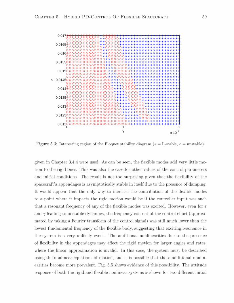
Chapter 5. Hybrid PD-Control Of Flexible Spacecraft 59
0 1 2
x 10−4
0.012
0.0125
0.013
0.0135
0.014
0.0145
0.015
0.0155
0.016
0.0165
0.017
γ
ε
Figure 5.3: Interesting region of the Floquet stability diagram (∗ = L-stable, = unstable).
given in Chapter 3.4.4 were used. As can be seen, the flexible modes add very little mo-
tion to the rigid ones. This was also the case for other values of the control parameters
and initial conditions. The result is not too surprising given that the flexibility of the
spacecraft’s appendages is asymptotically stable in itself due to the presence of damping.
It would appear that the only way to increase the contribution of the flexible modes
to a point where it impacts the rigid motion would be if the controller input was such
that a resonant frequency of any of the flexible modes was excited. However, even for ε
and γ leading to unstable dynamics, the frequency content of the control effort (approxi-
mated by taking a Fourier transform of the control signal) was still much lower than the
lowest fundamental frequency of the flexible body, suggesting that exciting resonance in
the system is a very unlikely event. The additional nonlinearities due to the presence
of flexibility in the appendages may affect the rigid motion for larger angles and rates,
where the linear approximation is invalid. In this case, the system must be described
using the nonlinear equations of motion, and it is possible that those additional nonlin-
earities become more prevalent. Fig. 5.5 shows evidence of this possibility. The attitude
response of both the rigid and flexible nonlinear systems is shown for two different initial

Chapter 5. Hybrid PD-Control Of Flexible Spacecraft 60
0 5 10 15−8
−7
−6
−5
−4
−3
−2
−1
0
1x 10
−6
# of Orbits
Qre
η
Figure 5.4: A plot showing the contribution of the flexible modes to the rigid ones.
conditions: for ω01 =[
0.0001 0.0001 0.0001]T
rads
and for ω02 =[
1 1 1]T
rads. The
control gains used were ε = 0.0001 and γ = 0.0035. For ω01, where the dynamics can
even be well-approximated by the linearized equations of motion, the attitude response
is almost exactly the same in both the rigid and flexible case. For ω02, the response of
the flexible spacecraft is seen to be much different than the rigid version, suggesting that
it is indeed the nonlinearities imposed by the flexibility of the system that is causing the
discrepancy. Thus, the linear Floquet analysis is limited in the sense that its stability
predictions may be invalid for larger angles and rates where the dynamics are no longer
linear. Chapter 5.3 investigates this issue in further detail.
The Floquet stability analysis was performed for various values of the appendages’
Young’s modulus E. Changing the stiffness did not alter the stability predictions. This
may be due to the very small impact the flexible modes have on the rigid ones. The
damping ratio was also varied and the stability predictions still remained the same. An
important observation is that even with zero damping (ζ = 0), the flexible modes (and
hence motion of the appendages) may still damp out even using purely magnetic control.
Recalling the modal equations of motion (see Chapter 3.4.4) and noting once again that

Chapter 5. Hybrid PD-Control Of Flexible Spacecraft 61
0 5 10−0.04
−0.02
0
0.02ω01
Qua
tern
ions
ǫ1ǫ2ǫ3
0 5 10−1
−0.5
0
0.5
1ω02
ǫ1ǫ2ǫ3
0 5 10−0.04
−0.02
0
0.02
Qua
tern
ions
# of Orbits
ǫ1ǫ2ǫ3
0 5 10−1
−0.5
0
0.5
1
# of Orbits
ǫ1ǫ2ǫ3
Figure 5.5: A plot illustrating the affect of flexibilty on the nonlinear system for larger anglesand rates. The top two plots are for the rigid spacecraft, and the bottom two are for the flexibleversion.
the eigenmatrix Q can be written as
Q =
[
1 Qre
0 Qee
]
,
and that q = Qη, the existence of Qre implies that the flexible modes contribute to the
rigid ones so that any flexible motion will cause the controller to provide a control torque
until the flexible modes are attenuated. The linear system was simulated using purely
magnetic control with ε = 0.0001 and ζ = 0, and the system response (including the tip
deflection ue(L) for one arm only) is shown in Fig. 5.6. As can be seen, even without the
help of physical damping the purely magnetic control law causes the tip deflection to go
to zero.
Another limitation of the Floquet analysis is that it says nothing about controller
performance. Fig. 5.7 shows the system response with the control gains set to ε =
0.0006853 and γ = 0.003191. As can be seen, although the dynamics will eventually
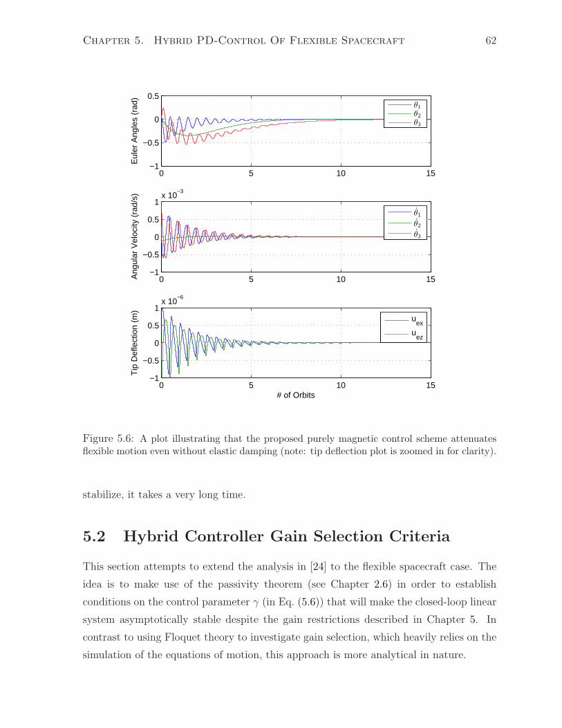
Chapter 5. Hybrid PD-Control Of Flexible Spacecraft 62
0 5 10 15−1
−0.5
0
0.5
Eul
er A
ngle
s (r
ad)
θ1
θ2
θ3
0 5 10 15−1
−0.5
0
0.5
1x 10
−3
Ang
ular
Vel
ocity
(ra
d/s)
θ1
θ2
θ3
0 5 10 15−1
−0.5
0
0.5
1x 10
−6
# of Orbits
Tip
Def
lect
ion
(m)
u
ex
uez
Figure 5.6: A plot illustrating that the proposed purely magnetic control scheme attenuatesflexible motion even without elastic damping (note: tip deflection plot is zoomed in for clarity).
stabilize, it takes a very long time.
5.2 Hybrid Controller Gain Selection Criteria
This section attempts to extend the analysis in [24] to the flexible spacecraft case. The
idea is to make use of the passivity theorem (see Chapter 2.6) in order to establish
conditions on the control parameter γ (in Eq. (5.6)) that will make the closed-loop linear
system asymptotically stable despite the gain restrictions described in Chapter 5. In
contrast to using Floquet theory to investigate gain selection, which heavily relies on the
simulation of the equations of motion, this approach is more analytical in nature.

Chapter 5. Hybrid PD-Control Of Flexible Spacecraft 63
0 20 40 60 80 100−0.05
0
0.05
Eul
er A
ngle
s (r
ad)
θ1
θ2
θ3
0 20 40 60 80 100−1
−0.5
0
0.5
1x 10
−4
Ang
ular
Vel
ocity
(ra
d/s)
# of Orbtis
θ1
θ2
θ3
Figure 5.7: A plot showing how the Floquet theory predicts stability but not controller per-formance.
For the rigid case, a completely analytic result can be obtained, imposing a condition
on the choice of γ in order to achieve stability for any ε. It is shown in Appendix B that
stability for the closed-loop rigid system using the hybrid control scheme is achieved as
long as γ > kpk2d
λmax, where λmax is the spacecraft’s largest principle inertia.
For the flexible case, a similar procedure (as in [24] and Appendix B) is performed in
order to establish gain selection criteria. Consider, once again, the closed-loop equations
of motion for the flexible linear system given by Eqs. (3.12) and (5.6), which can be
written collectively as
Mq + Dq + Kq = −B(ε2kpq + εkdq
).
With the intention of decoupling the dynamics as much as possible, and of obtaining
simpler equations to work with the above equations are cast into modal coordinates
η = Q−1q (as shown in Chapter 3.4.4), yielding the transformed equations which are
written as
Mmodη + Dmodη + Kmodη = −QTBQ(ε2kpη + εkdη
), (5.7)

Chapter 5. Hybrid PD-Control Of Flexible Spacecraft 64
where
Mmod =
[
I 0
0 1
]
, Dmod =
[
0 0
0 2ζΩ
]
, and Kmod =
[
0 0
0 Ω2
]
.
It is important to note that Dmod and Kmod are diagonal matrices and that Mmod can be
made diagonal (i.e., making I diagonal) by either choosing the body frame to coincide
with the spacecraft’s principal axes or by normalizing Q such that I is diagonalized. Also,
the control matrix B can be written as
B =
[
(µγ1+ Γ) 0
0 µM ee
]
+
[
(1− µ)γ1 0
0 −µM ee
]
,
where 0 < µ < 1. The closed-loop system can be decomposed into a traditional plant
and controller type structure (as shown in Figs. 2.2 and 2.3). The plant’s output, y(t),
is defined as
y(t) = εkdη(t) + ε2kpη(t),
and its control input, u(t), as
−u(t) = QT
[
(µγ1+ Γ) 0
0 µM ee
]
Q
︸ ︷︷ ︸
H(t)
y(t).
Defining the control input in this way removes the time-varying part of the closed-loop
system from the plant dynamics. Furthermore, the mapping between controller input y
and controller output u, denoted by the operator H, is then strictly passive since
∫ T
0
yT (Hy) dt =∫ T
0
yTΘ(t)y(t) dt
≥ σmin
∫ T
0
yTy dt,
where
Θ(t) = QT
[
(µγ1+ Γ(t)) 0
0 µM ee
]
Q > 0,
and σmin is the smallest eigenvalue of Θ. Note that Θ is positive definite for any t > 0
since (µγ1+ Γ) and M ee are both positive definite. Thus, the operator H simply corre-
sponds to time-varying negative feedback using a positive definite gain matrix, which is

Chapter 5. Hybrid PD-Control Of Flexible Spacecraft 65
strictly passive (as shown). The passivity theorem then requires that the plant, described
by the operator G, be passive in order to guarantee input-output stability. With these
definitions for input and output, Eq. (5.7) can be written as
Mmodη(t) + Dmodη(t) + Kmodη(t) = u(t)−Ξy(t),
where
Ξ = QT
[
(1− µ)γ1 0
0 −µM ee
]
Q.
Since the above system is LTI, it can be described in the frequency domain by a transfer
matrix. To this end, a Laplace transform (with the transform variable denoted by s) is
performed, giving
(s2Mmod + sDmod + Kmod
)η(s) +Ξy(s) = u(s).
Noting that y(s) = (εkds+ ε2kp)η(s), the resulting system can be written as
(s2Mmod + sDmod + Kmod
εkds+ ε2kp
)
y(s) +Ξy(s) = u(s)
y(s) =[(
s2Mmod + sDmod + Kmod
εkds+ ε2kp
)
+Ξ
]−1
︸ ︷︷ ︸
G(s)
u(s)
y(s) = G(s)u(s).
The plant is therefore described by the transfer matrix G(s) as defined above. Fig. 5.8
shows the block diagram representation of the closed-loop system. It is of the same form
as the generic system in Fig. 2.3, for which the passivity theorem was derived. It is
important to note that each element of G(s) is a real and rational function of s. It is
known that an LTI operator (such as G) is passive if its corresponding transfer matrix
G(s) is positive real (PR). Finding conditions for which the plant is PR would then mean
that the requirements for L2-stability are satisfied via the passivity theorem. According
to [34], G(s) is PR if and only if
(a) no element of G(s) has a pole in Res ≥ 0;
(b) GH(jω) + G(jω) ≥ 0 for all real ω, with jω not a pole of any element of G;

Chapter 5. Hybrid PD-Control Of Flexible Spacecraft 66
+
−
0 y
−u
H(t)
G(s)
QT
[
(µγ1+ Γ(t)) 0
0 µMee
]
Q
Figure 5.8: Block diagram for the flexible, hybrid-controlled system.
(c) for any jω0 that is a pole for some element of G, it is at most a simple pole, and the
residue matrix, given by K 0 = lims→jω0
(s− jω0)G(s) for finite ω0 and K∞ = limω0→∞
G(jω0)jω0
if ω0 is infinite, is non-negative definite Hermitian,
where (·)H refers to the conjugate transpose operation for a complex-valued matrix. Note
that in G, there are damping terms for both the rigid and flexible components; the rigid
damping coming from the rate feedback of the control law and the flexible damping
inherent in the physical spacecraft structure itself. The presence of this damping is
enough to ensure that there are no purely imaginary poles, and so condition (c) is satisfied
automatically. Condition (b) can be satisfied using adequate choices for the control
parameters. The control parameters can be estimated numerically by fixing ε, kp, and
kd, and finding the minimum γ such that GH(jω) + G(jω) ≥ 0 for a large range of
ω. The other parameters may be changed and the procedure repeated. Fig. 5.9 shows
the minimum value of γ satisfying (b) over a range of ε (with kp = 25000 kg·m2
s2and
kd = 25000 kg·m2
s) for the sample system given in Chapter 3.5. For each pair of ε and γ
in Fig. 5.9, condition (a) was verified numerically using the pole() function in MATLAB.
Therefore, the graph obtained shows values for the control parameters ensuring G is PR,
implying that the system given by Eq. (5.3) is input-output stable.
Lyapunov stability can also be shown, assuming that G is PR. A minimal realization
of G can be written as G(s) = C (s1− A)−1 B, for some matrices A,B,C. Letting
x =[
ηT ηT
]T
, a state-space representation of the block diagram in Fig. 5.8 can be
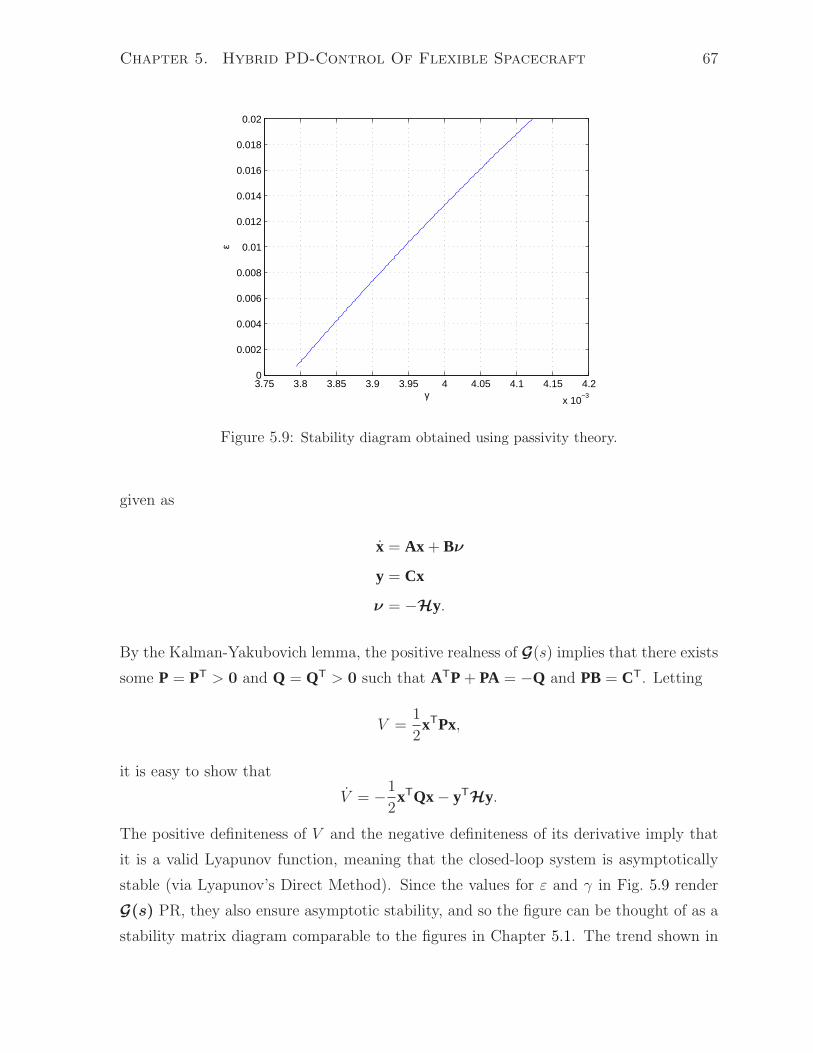
Chapter 5. Hybrid PD-Control Of Flexible Spacecraft 67
3.75 3.8 3.85 3.9 3.95 4 4.05 4.1 4.15 4.2
x 10−3
0
0.002
0.004
0.006
0.008
0.01
0.012
0.014
0.016
0.018
0.02
γ
ε
Figure 5.9: Stability diagram obtained using passivity theory.
given as
x = Ax + Bν
y = Cx
ν = −Hy.
By the Kalman-Yakubovich lemma, the positive realness of G(s) implies that there exists
some P = PT > 0 and Q = QT > 0 such that ATP+ PA = −Q and PB = CT. Letting
V =1
2xTPx,
it is easy to show that
V = −1
2xTQx − yT
Hy.
The positive definiteness of V and the negative definiteness of its derivative imply that
it is a valid Lyapunov function, meaning that the closed-loop system is asymptotically
stable (via Lyapunov’s Direct Method). Since the values for ε and γ in Fig. 5.9 render
G(s) PR, they also ensure asymptotic stability, and so the figure can be thought of as a
stability matrix diagram comparable to the figures in Chapter 5.1. The trend shown in

Chapter 5. Hybrid PD-Control Of Flexible Spacecraft 68
Fig. 5.9 shows a very conservative estimate for the minimum γ needed to ensure stability
at a particular ε, when compared to Fig. 5.1. It is clear that this passivity analysis yields
sufficient, though not neccesary, conditions on γ, since choosing γ = 0.0038 would ensure
stability for any ε. An example validating this analysis can be seen in Fig. 5.10, where
the spacecraft’s unstable motion under purely magnetic control (with ε = 0.003) is shown
to become stable when choosing γ = 0.0038 as predicted by Fig. 5.9. Note that Floquet
theory estimated that stability is obtained for γ ≈ 0.0012.
0 1 2−5
0
5
10x 10
5 ǫ = 0.003, γ = 0
Eul
er A
ngle
s (r
ad)
θ1
θ2
θ3
0 1 2−0.2
−0.1
0
0.1
0.2ǫ = 0.003, γ = 0.0038
θ1
θ2
θ3
0 1 2−2000
−1000
0
1000
2000
Ang
ular
Vel
ocity
(ra
d/s)
# of Orbits
θ1
θ2
θ3
0 1 2−5
0
5
10x 10
−4
# of Orbits
θ1
θ2
θ3
Figure 5.10: A plot illustrating the validity of the hybrid gain selection criteria. Purelymagnetic control on the left, hybrid control on the right.
This passivity analysis was performed for various values of the damping ratio and
the Young’s modulus as well. Larger damping ratios gave less conservative results. For
example, given ε = 0.003, with ζ = 0.1 stability was achieved if γ ≈ 0.00381, but with
ζ = 0.5 all that was needed was that γ = 0.00376. When the Young’s modulus was
increased, a single value for γ was obtained for all ε. With E = 4 × 10¹¹ Pa, the single
value for γ obtained was γ = 0.00791. It is clear that changing the material properties
of the flexible appendages does have a small affect on the passivity analysis. The more
“rigid” the appendages were made to be, the closer the analysis results were to the rigid

Chapter 5. Hybrid PD-Control Of Flexible Spacecraft 69
case as is expected. It is important to note that a stabilizing γ could not be found
for some values of the material properties. A reason for the analysis breaking down is
discussed below, where it shown that for weak coupling between the flexible and rigid
modes there are simultaneous bounds on γ and ε.
A more analytical result may be obtained if it is assumed that the coupling between
the flexible and rigid modes is weak. Noting once again that the eigenmatrix Q can be
written as
Q =
[
1 Qre
0 Qee
]
,
the weak-coupling assumption amounts to saying that the Qre term is negligible. The
transfer matrix G(s) is then completely decoupled, and the rigid and flexible dynamics
can be investigated independently. With this assumption,
G(s) ≈
[
1
εkds+ ε2kp
(
s2
[
I 0
0 1
]
+ s
[
0 0
0 2ζΩ
]
+
[
0 0
0 Ω2
])
+
[
(1− µ)γ1 0
0 −µ1
]]−1
,
where, in each matrix the top-left quadrant represents the rigid dynamics, and the
bottom-right represents the flexible dynamics. Once again, it is necessary to find condi-
tions on the parameters in G such that it is positive real (which would then imply that
it is also passive). Since it is diagonal, this requirement implies that each of its elements,
Gi(s), must be positive real. As shown in [35], Gi(s) is strictly positive real (SPR, which
is a stronger condition implying positive realness) if
(a) it is analytic in Res ≥ 0;
(b) ReGi(jω) > 0, for ω ∈ (−∞,∞);
(c) limω→∞
ω2ReGi(jω) > 0.
For the rigid subsystem, Appendix B shows that all three conditions are met for each
of its elements if
kp > 0, kd > 0, ε > 0, µ < 1, and γ >kp
k2dλmax, (5.8)
where λmax is the largest principal moment of inertia. It is important to note that this
bound on γ differs from that in [24] by a factor of λmax since the moment of inertia was
not included in the control law.

Chapter 5. Hybrid PD-Control Of Flexible Spacecraft 70
For the flexible subsystem, each element of the transfer matrix becomes
Gi(s) =
[s2 + 2ζωis+ ω2
i
εkds+ ε2kp− µ
]−1
.
Letting µ→ 0 and s = jω it can be shown that
Gi(jω) =[ε2kp (ω
2i − ω2) + 2εkdζωiω
2] + j [εkdω (ω2i − ω2)− 2ε2kpζωiω]
(ω2i − ω2)
2+ (2ζωiω)
2,
from which it is easy to show that
limω→∞
ω2ReGi(jω) = 2εkdζωi − ε2kp.
Condition (a) is automatically satisfied if γ > 0, kp > 0, kd > 0, ǫ > 0, and µ < 1. From
the above equation, it is clear that condition (c) is satisfied if ε < 2ζωikdkp. To satisfy
condition (b), ε must be chosen such that 2kdζωiω2 + εkpω
2i > εkpω
2. If the bound on ε
from condition (c) holds, then the above inequality is also satisfied since
ε < 2ζωikd
kp⇒ εkpω
2 < 2ζkdωiω2 < 2ζkdωiω
2 + εkpω2i .
To summarize, after imposing the weak-coupling assumption, each element of G (and
hence G itself) is SPR if
kp > 0, kd > 0, µ < 1, γ >kp
k2dλmax, and 0 < ε < 2ζωmin
kd
kp,
where ωmin is the lowest natural frequency of the flexible system. Therefore, if these
bounds on the control parameters hold, then the closed loop system is input-output
stable. Asymptotic stability can also be shown in a similar way as was done for the
coupled case.
With kp = 25000 kg·m2
s2and kd = 25000 kg·m2
s, the gain selection criteria given by the
above conditions are that 0 < ε < 0.406 and γ > 0.00378 in order to guarantee stability.
When compared to the stability map (Fig. 5.1) predicted using Floquet analysis, this
selection criteria provides a conservative method of choosing the control gains. When
compared to the stability diagram obtained using passivity theory (see Fig. 5.9) for
the case where the weak-coupling assumption was not imposed, the stability criteria

Chapter 5. Hybrid PD-Control Of Flexible Spacecraft 71
agrees and gives a slightly less conservative estimate. This agreement with the other
stability analyses suggests that using the weak-coupling assumption to obtain analytically
obtainable stability criteria is a valid and useful approach. The value in using this
analytical approach is that it provides a very quick and relatively easy way to place
conditions on the control gains ensuring stability, which is vital in control design.
Since there is an explicit bound on the gains it is easy to see what the effects of elastic
damping and material stiffness would be on the stability of the system. The bound on
γ is independent of both of those properties, and so would remain the same. The bound
on ε depends on both the damping ratio and the minimum natural frequency of the
appendages. It is clear that increasing the damping or stiffness properties of the flexible
structure will raise the upper bound on ε.
5.3 Stability of the Nonlinear System
The stability of the hybrid controller developed in the preceding sections was proven
for the linearized system. This section will explore how well the stability predictions
(obtained using the linear Floquet analysis) apply to the nonlinear equations of mo-
tion. Recall that the closed-loop, flexible nonlinear dynamics are described by Eqs. (3.9)
and (3.10), where fe = 0, and τ (which in this case represents the hybrid control law) is
given by
τ = −(γ1+ Γ)(2ε2kpǫ+ εkdω
).
In general, the linearization of a nonlinear system accurately describes the dynamics
only when the state variables and initial conditions differ from the equilibrium point
by small values. For initial conditions outside of the linear approximation range, the
linearized system does not accurately describe the dynamics. Fig. 5.11 shows a compar-
ison of the state response of both the linear and nonlinear system for initial conditions
that are within, and outside, of the linear approximation range. The control parameters
used were ε = 0.0001 and γ = 0.0038 with kp and kd the same as in Chapter 5.1. The
initial conditions were ω01 =[
0.0001 0.0001 0.0001]T
rads, which is within the linear
approximation range, and ω01 =[
0.1 0.1 0.1]T
rads, which is outside it. All other state
variables were initially zero. As can be seen, for ω01 the linear system accurately describes
the nonlinear dynamics but for ω02, they are very different. Although not plotted, the
flexible degrees of freedom (qe) followed the same trend. This is a limitation of designing

Chapter 5. Hybrid PD-Control Of Flexible Spacecraft 72
a control law for a nonlinear system around its linearization. When evaluating if the
stability analyses based on the linear system apply in the nonlinear case, it is important
to keep this limitation in mind.
0 5 10−0.04
−0.02
0
0.02
Eul
er A
ngle
s (θ
/2 r
ad)
θ1
θ2
θ3
0 5 10−1
0
1
2x 10
−4
Ang
ular
Vel
ocity
(ra
d/s)
θ1
θ2
θ3
0 5 10−0.04
−0.02
0
0.02
Qua
tern
ions
# of Orbits
ǫ1ǫ2ǫ3
0 5 10−1
0
1
2x 10
−4
Ang
ular
Vel
ocity
(ra
d/s)
# of Orbits
ω1
ω2
ω3
0 5 10−40
−20
0
20
Eul
er A
ngle
s (θ
/2 r
ad)
θ1
θ2
θ3
0 5 10−0.1
0
0.1
Ang
ular
Vel
ocity
(ra
d/s)
θ1
θ2
θ3
0 5 10−1
0
1
Qua
tern
ions
# of Orbits
ǫ1ǫ2ǫ3
0 5 10−0.2
0
0.2
Ang
ular
Vel
ocity
(ra
d/s)
# of Orbits
ω1
ω2
ω3
Figure 5.11: A plot comparing the system response for initial conditions in, and outside, thelinear approximation range. The top four plots have an initial angular velocity of ω01, and thebottom four have an intial angular velocity of ω02.

Chapter 5. Hybrid PD-Control Of Flexible Spacecraft 73
The closed-loop linear and nonlinear system dynamics were simulated for various
values of ε and γ along the stability boundaries seen in Figs. 5.1 and 5.3. The L-
stability of the dynamics was deduced by inspection. Table 5.1 shows a comparison
between the predicted stability (using Floquet theory), the linear system response, and
the nonlinear system response for both initial conditions (ω01 and ω02). It is important
to note that the linear dynamics are not accurate for ω02, but are included anyways.
Floquet theory predicts the stability (of the linear system) for any initial condition,
even those such that the dynamics are no longer linear. Thus, as seen in Table 5.1, the
simulated linear response confirms the Floquet prediction even for ω02, which is outside
the linear approximation range. An example of a stable and unstable response for the
Table 5.1: Comparison between the Floquet stability prediction, and the simulated lin-ear/nonlinear response.
ε γFloquet ω01 ω02
Prediction Linear Nonlinear Linear∗ Nonlinear0.0001 0 stable stable stable stable stable
0.0006853 0 unstable unstable unstable unstable unstable0.0006853 0.003088 unstable unstable unstable unstable unstable0.0006853 0.003191 stable stable stable stable stable0.001856 0.001441 unstable unstable unstable unstable unstable0.002441 0.001647 stable stable stable stable stable0.006538 0.0003088 unstable unstable unstable unstable unstable0.006538 0.0004118 stable stable stable stable stable0.01217 0.000145 unstable unstable unstable unstable unstable0.0155 0.000065 unstable unstable unstable unstable unstable0.0155 0.000075 stable stable stable stable stable0.0155 0.00009 unstable unstable unstable unstable unstable0.01533 0.00011 stable stable stable stable stable0.01824 0.003191 stable stable stable stable stable
Note: the term “stable” as used here means “asymptotically stable”.∗The linear system response is not accurate for this initial condition.
nonlinear system can be seen in Fig 5.12, where the conditions in rows 2 (unstable) and 8
(stable) of Table 5.1 were simulated with ω02 as an initial angular velocity. Note that the
tip deflection for only one appendage is shown. Table 5.1 also shows that the stability
of the nonlinear dynamics matched the Floquet prediction, suggesting that the linear
stability analysis might be able to predict the stability of the nonlinear system, even for
larger angles and rates. This, of course, is merely a suggestion and does not constitute a
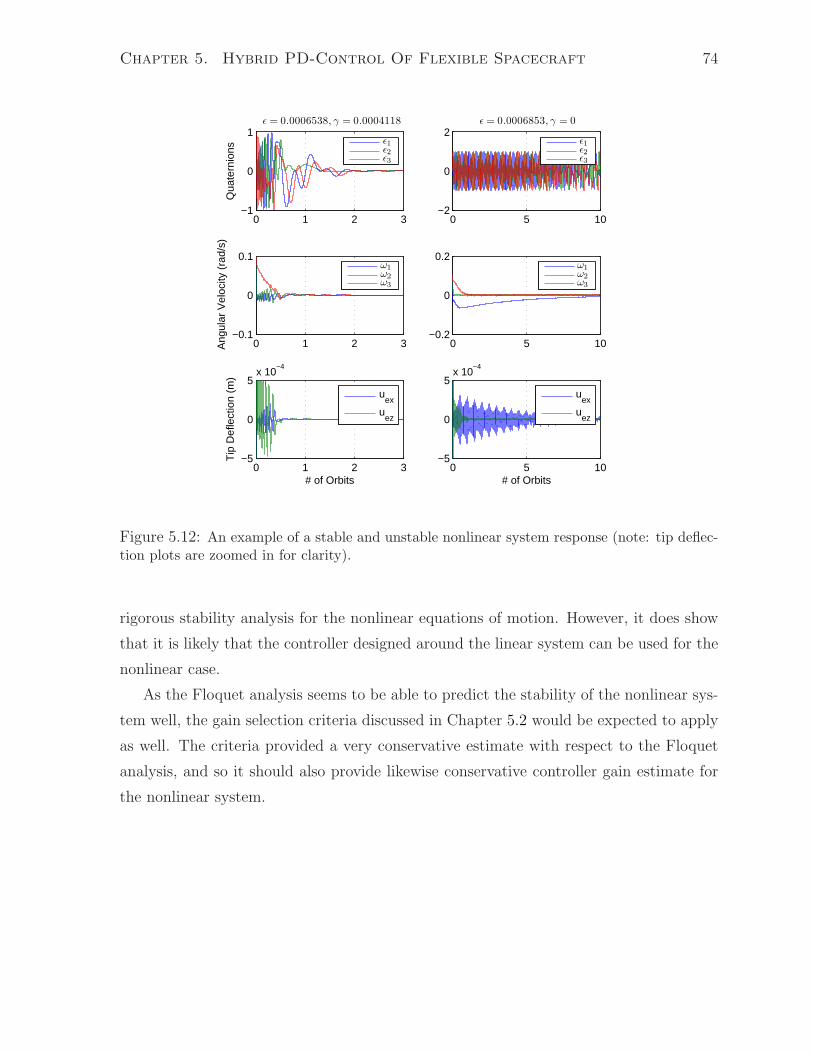
Chapter 5. Hybrid PD-Control Of Flexible Spacecraft 74
0 1 2 3−1
0
1ǫ = 0.0006538, γ = 0.0004118
Qua
tern
ions
ǫ1ǫ2ǫ3
0 5 10−2
0
2ǫ = 0.0006853, γ = 0
ǫ1ǫ2ǫ3
0 1 2 3−0.1
0
0.1
Ang
ular
Vel
ocity
(ra
d/s)
ω1
ω2
ω3
0 5 10−0.2
0
0.2
ω1
ω2
ω3
0 1 2 3−5
0
5x 10
−4
# of Orbits
Tip
Def
lect
ion
(m)
u
ex
uez
0 5 10−5
0
5x 10
−4
# of Orbits
u
ex
uez
Figure 5.12: An example of a stable and unstable nonlinear system response (note: tip deflec-tion plots are zoomed in for clarity).
rigorous stability analysis for the nonlinear equations of motion. However, it does show
that it is likely that the controller designed around the linear system can be used for the
nonlinear case.
As the Floquet analysis seems to be able to predict the stability of the nonlinear sys-
tem well, the gain selection criteria discussed in Chapter 5.2 would be expected to apply
as well. The criteria provided a very conservative estimate with respect to the Floquet
analysis, and so it should also provide likewise conservative controller gain estimate for
the nonlinear system.

Chapter 6
Conclusions
The purpose of this thesis was to investigate using magnetic actuators for the attitude
control of a flexible spacecraft. The PD-like magnetic control techniques previously used
for rigid spacecraft were extended to the flexible case. The gain limitations inherent
with this type of control are shown to be alleviated with the addition of a minimum
amount of control effort from an alternate, independent, three-axis actuation system
(such as reaction wheels or thrusters). The hybrid control law in [24] designed for a rigid
spacecraft was adopted and modified for the flexible case.
The relevant background concepts needed to understand and investigate the control
problem were presented. A brief summary of the notation used throughout the thesis
was given, as it was critical in the development of the equations of motion. Spacecraft
“attitude” was defined using a rotation matrix, and two parameterizations (Euler angles
for the linear dynamics, quaternions for the nonlinear dynamics) were presented. The two
main definitions of stability (input-ouput and Lyapunov) were also stated, and several
stability theories used in the closed-loop system’s stability analyses were summarized:
Floquet, Lyapunov, and passivity theory.
The mechanics of a flexible spacecraft in an orbit around the earth was then devel-
oped. A geocentric inertial reference frame and a frame affixed to the spacecraft body
were defined in order to describe the mechanics. Since magnetic attitude control requires
knowledge of the geomagnetic field at a particular point along the spacecraft’s orbit, the
orbit definition and mechanics in terms of orbital elements was presented. Quaternions
were used to represent the spacecraft kinematics, which describes the evolution of the
spacecraft’s orientation over time. Vectrix notation was used to develop the dynamical
equations of motion for both a rigid and flexible spacecraft. The flexibility of the space-
75
Chapter 6. Conclusions 76
craft was incorporated using the Rayleigh-Ritz method, where the elastic deflections of
the body are represented by a series of shape functions describing the deformation field
coupled with generalized coordinates for the deformation degrees of freedom. The lin-
earized equations of motion were also derived, as the controller development and stability
analyses focused on the linear dynamics. The linearized system was further broken down
into modal coordinates, so that the rigid and flexible modes could be analyzed indepen-
dently. An example spacecraft consisting of a rigid hub with two flexible appendages
attached was presented as an archetype.
A model for the earth’s magnetic field was presented. It assumes that the magnetic
field can be represented by the gradient of a scalar potential function consisting of a
series of spherical harmonics. Controllability of the spacecraft magnetic attitude control
problem was discussed. It was shown that the spacecraft is instantaneously underac-
tuated since the interaction between the geomagnetic field and a dipole created by the
magnetic actuators is governed by a vector cross product. However, if the magnetic field
experienced by the spacecraft varies enough along the orbit, the attitude dynamics can be
controllable in a time-varying sense. The constant dipole approximation of the geomag-
netic field (obtained by taking the first harmonic only of the spherical harmonic model)
is able to satisfy the controllability requirements, and is the model that was adopted for
this thesis. The requirements also suggest that magnetic attitude control is best suited
for spacecraft in low-earth and polar orbits. After establishing controllability, a more
indepth summary of the PD-like control law designed for rigid spacecraft was explored
since the controller design for flexible spacecraft was based on it. Limitations on the
gains for this type of control were shown to exist, and a hybrid control scheme (for the
rigid case) that relaxes these limitations was presented.
These rigid controllers were then extended to the flexible case. A PD-like control law
was proposed for the linear system. The lack of any spacecraft properties (i.e., moment
of inertia) in the controller made it more robust than the one for the rigid case (on which
it was based). Stability of the closed-loop system was explored and it was shown that
the gain limitations still exist. A hybrid controller was then proposed that augments
the purely magnetic control with an alternate, independent, three-axis actuation system.
Floquet analysis was used to determine how much effort the additional actuation system
needed to provide in order to ensure stability. It was seen that as the control gains for
the purely magnetic control increased, less control effort was needed from the additional
actuation system. The Floquet analysis also provided a stability map that could be used

Chapter 6. Conclusions 77
for hybrid controller design. Floquet analysis was also performed on the rigid version
of the archetypal spacecraft and it was seen that the stability predictions were identical
to the flexible case. This suggests it might be possible that controllers designed for the
rigid system can be adopted for the flexible case “as is”. The modal equations of motion
were used to show that the flexible modes had little effect on the rigid ones using the
hybrid control scheme. Even when both the damping ratio and stiffness (represented by
the Young’s modulus) were varied, the Floquet predictions did not change.
Passivity theory was used in order to obtain gain selection criteria for the hybrid
controller. The closed-loop system was decomposed into a linear time-invariant plant
with a time-varying strictly passive feedback. Conditions on the control gains were
then obtained (numerically) that made the plant passive and hence, the closed-system
input-output stable. Asymptotic stability was shown to follow from the input-output
result. Making the assumption that the flexible modes contribute little to the rigid ones
allowed for bounds on the control gains to be obtained analytically. The Floquet analysis
confirmed the validity of these bounds, and so the analytical gain criteria and passivity
analysis proved to be a relatively effective tool for the practical design of a controller
using the hybrid control scheme.
The hybrid controller proposed in this thesis was based on the linear system dynamics.
The stability of the nonlinear closed-loop system was investigated via simulation. The
stability predictions based on the Floquet and passivity analyses were tested. It was
found that the Floquet predictions for the linear system also predicted the stability of
the nonlinear system, even for angles and rates outside the linear approximation range. It
was concluded that the hybrid PD-like controller design for the actual nonlinear system
could be based on the linearized version, meaning that the gain selection criteria and
stability maps obtained via the linear analyses would likely apply to the nonlinear case.
6.1 Future Work
This thesis aims at providing a design method for a particular class of control. The main
drawback of using the purely magnetic control is the gain limitations embodied in the
existence of ε∗. This gain limitation was estimated using numerical analyses; finding
a way to calculate it analytically would be an important addition to the work done in
this thesis. The analyses performed focused on determining the gain values that would
lead to a stable system without regard for controller performance. Investigating the gain

Chapter 6. Conclusions 78
criteria for optimal controller performance would be another great contribution. The
stability analyses all focused on the linear system dynamics, and so the controller had to
be design around the linear system as well. The nonlinear system stability was inferred
in a non-rigorous way. Finding a technique that analyzes the stability of the nonlinear
system would make the results of this thesis applicable to a broader range of motion.
Future work could also include examining the situation where the sensors and actua-
tors are not collocated, as they are assumed to be in this thesis. Non-collocated sensors
and actuators would potentially introduce destabilizing spillover from flexible modes that
have not been accounted for in the spacecraft model. Also, there are other ways of de-
scribing the flexibility of a body, and an investigation of these other methods might lead
to more insight regarding the flexible dynamics. Another limitation of the work done in
this thesis is that the spacecraft was axisymmetric, and so the deflections caused by rigid
motion would contain symmetry as well. Extending the controller design for spacecraft
that are not symmetric would be interesting.
This thesis deals primarily with PD-like control. Future work could include extending
other types of control methods (such as the ones briefly mentioned in Chapter 1.1) to
the flexible case, and comparing them among each other to see if any particular control
technique allows for easier design.

References
[1] J. Wertz, Spacecraft Attitude Determination and Control. D. Reidel Publishing Co.,Dordrecht, The Netherlands, 1978.
[2] S. Bhat and A. Dham, “Controllability of spacecraft attitude under magnetic actu-ation,” in IEEE Conference on Decision and Control, 2003.
[3] E. Silani and M. Lovera, “Magnetic spacecraft attitude control: a survey and somenew results,” Control Engineering Practice, vol. 13, pp. 357–371, 2005.
[4] R. Ryan, “Simulation of actively controlled spacecraft with flexible appendages,”Journal of Guidance, Control, and Dynamics, vol. 13, no. 4, pp. 691–702, 1990.
[5] H. Bang, C. Ha, and J. Kim, “Flexible spacecraft attitude maneuver by applicationof sliding mode control,” Acta Astronautica, vol. 57, pp. 841–850, 2005.
[6] S. Bhat, “Controllability of nonlinear time-varying systems: Applications to space-craft attitude control using magnetic actuation,” IEEE Transactions on Automatic
Control, vol. 50, no. 11, pp. 1725–1735, 2005.
[7] R. Wisniewski and M. Blanke, “Fully magnetic attitude control for spacecraft subjectto gravity gradient,” Automatica, vol. 35, pp. 1201–1214, 1999.
[8] C. Damaren, “Comments on: Fully magnetic attitude control for spacecraft subjectto gravity gradient,” Automatica, vol. 38, p. 2189, 2002.
[9] R. Wisniewski, “Linear time-varying approach to satellite attitude control using onlyelectromagnetic actuation,” Journal of Guidance, Control, and Dynamics, vol. 23,no. 4, pp. 640–647, 2000.
[10] M. Psiaki, “Magnetic torquer attitude control via asymptotic periodic linearquadratic regulation,” Journal of Guidance, Control, and Dynamics, vol. 24, no. 2,pp. 386–394, 2001.
[11] M. Lovera, E. D. Marchi, and S. Bittanti, “Periodic attitude control techniques forsmall satellites with magnetic actuators,” IEEE Transactions on Control Systems
Technology, vol. 10, no. 1, pp. 90–95, 2002.
[12] J. Kulkarni and M. Campbell, “An approach to magnetic torque attitude control ofsatellites via ‘H∞’ control for LTV systems,” in 43rd IEEE Conference on Decision
and Control, 2004.
79

References 80
[13] M. Lovera and A. Astolfi, “Global magnetic attitude control of inertially pointingspacecraft,” Journal of Guidance, Control, and Dynamics, vol. 28, no. 5, pp. 1065–1067, 2005.
[14] M. Lovera and A. Astolfi, “Global magnetic attitude control of spacecraft in the pres-ence of gravity gradient,” IEEE Transactions on Aerospace and Electronic Systems,vol. 42, no. 3, pp. 796–805, 2006.
[15] A. Astolfi and M. Lovera, “Global spacecraft attitude control using magnetic actu-ators,” in Proceedings of the American Control Conference, pp. 1331–1335, 2002.
[16] M. Lovera and A. Astolfi, “Spacecraft attitude control using magnetic actuators,”Automatica, vol. 40, pp. 1405–1414, 2004.
[17] H. K. Khalil, Nonlinear Systems. Prentice Hall, Upper Saddle River, NJ, 1996.
[18] J. Liang, R. Fullmer, and Y. Chen, “Time-optimal magnetic attitude control forsmall spacecraft,” in 43rd Conference on Decision and Control, pp. 255–260, 2004.
[19] M. Lovera and A. Varga, “Optimal discrete-time magnetic attitude control of satel-lites,” in Proceedings of the 16th IFAC World Congress, 2005.
[20] S. Sakai, Y. Fukushima, and H. Saito, “Studies on magnetic attitude control systemfor the reimei microsatellite,” in AIAA, 2006.
[21] J. Oh, S. Park, and K. Choi, “Magnetic torque attitude control of a satellite usingthe state-dependent riccati equation technique,” in AIAA Guidance, Navigation,
and Control Conference and Exhibit, 2006.
[22] T. Pulecchi and M. Lovera, “Attitude control of spacecraft with partially magneticactuation,” in IFAC Symposium on Automatic Control in Aerospace, vol. 17, 2007.
[23] J. Forbes and C. Damaren, “Geometric approach to spacecraft attitude control usingmagnetic and mechanical actuation,” Journal of Guidance, Control, and Dynamics,vol. 33, no. 2, pp. 590–595, 2010.
[24] C. J. Damaren, “Hybrid magnetic attitude control gain selection,” Proc. IMechE,
Part G, J. of Aerospace Engineering, vol. 223, pp. 1041–1047, 2009.
[25] F. Schiavo, M. Lovera, and A. Astolfi, “Magnetic attitude control of spacecraft withflexible appendages,” in 43rd IEEE Conference on Decision and Control, pp. 1545–1550, 2006.
[26] P. Hughes, Spacecraft Attitude Dynamics. Dover Publications Inc., Mineola, NY,2004.
[27] C. Chicone, Ordinary Differential Equations with Applications. Springer-Velag NewYork Inc., 1999.
References 81
[28] C. J. Damaren, “AER1503H Spacecraft Dynamics and Control 2 Course Notes,”tech. rep., University of Toronto Institute for Aerospace Studies, 2010.
[29] C. Desoer and M. Vidyasagar, Feedback Systems: Input-Output Properties. AcademicPress Inc., 1975.
[30] C. J. Damaren, “AER506H Spacecraft Dynamics and Control 1 Course Notes,” tech.rep., University of Toronto Institute for Aerospace Studies, 2009.
[31] J. DeLaurier, “AER503H Aeroelasticity Course Notes,” tech. rep., University ofToronto Institute for Aerospace Studies, 2007.
[32] C. C. Finlay, S. Maus, C. D. Beggan, and T. N. Bondar, “International geomagneticreference field: Eleventh generation,” Geophysical Journal International, vol. 183,pp. 1216–1230, October 2010.
[33] S. Chee, “Stability of a hybrid magnetic attitude control system,” Master’s thesis,University of Toronto Institute for Aerospace Studies, 2009.
[34] B. Anderson and S. Vongpanitlerd, Network Analysis And Synthesis. Dover Publi-cations Inc., Mineola, NY, 2006.
[35] P. Ioannou and G. Tao, “Frequency domain conditions for strictly positive realfunctions,” IEEE Transactions on Automatic Control, vol. 32, pp. 53–54, 1987.
[36] B. Wie, Space Vehicle Dynamics and Control. Washington, DC: AIAA, 1998.

Appendix A
Geomagnetic Field Model
Supplemental Calculations
The transformed Gaussian coefficients gn,m and hn,m are defined as
gn,m ≡ Sn,mgmn
hn,m ≡ Sn,mhmn ,
where
Sn,m ≡
[(2− δ0m)(n−m)
(n+m)
]1/2(2n− 1)!!
(n−m)!.
The parameter δ0m = 1 if m = 0, and is 0 otherwise. The Gauss functions P n,m can be
obtained recursively by noting that
P 0,0 = 1
P n,n = sin(θ)P n−1,n−1
P n,m = cos(θ)P n−1,m −Kn,mP n−2,m,
where
Kn,m ≡
(n−1)2−m2
(2n−1)(2n−3)n > 1
0 n = 1.
82

Appendix A. Geomagnetic Field Model Supplemental Calculations 83
The partial derivatives of the Gauss functions can also be obtained recursively:
∂P 0,0(θ)
∂θ= 0
∂P n,n(θ)
∂θ= sin(θ)
∂P n−1,n−1(θ)
∂θ+ cos(θ)P n−1,n−1 n ≥ 1
∂P n,m(θ)
∂θ= cos(θ)
∂P n−1,m(θ)
∂θ− sin(θ)P n−1,m −Kn,m∂P
n−2,m(θ)
∂θ.

Appendix B
Hybrid Control Gain Selection For
Rigid Spacecraft
This section outlines the proof of the stability condition on γ in the rigid spacecraft
version of the hybrid magnetic control scheme presented in Chapter 5. It closely follows
the analysis in [24] which is the basis of the proposed control law.
Consider a spacecraft system controlled using both magnetic actuation as well as
another three-axis control actuator (i.e., thrusters). This system can be described by the
equations (see Chapters 3 and 4.3)
˙q =1
2
[
q41+ q×
−qT
]
ω
I ω + ω×Iω = u + τ , (B.1)
where q =[
qT q4
]T
are the quaternions representing the spacecraft attitude, ω is the
spacecraft angular velocity, u is the control due to the alternate three-axis actuation
system and τ is due to the magnetic control all in the body frame. Consider the control
law given by
u = −γ[ǫkdω + 2ǫ2kpq
](B.2)
and
τ = −b×m
m = ‖bi‖−2 b×ν
ν = −[ǫkdω + 2ǫ2kpq
], (B.3)
84

Appendix B. Hybrid Control Gain Selection For Rigid Spacecraft 85
where b and bi is the geomagnetic field vector in the body and geocentric inertial frame,
respectively. Note that this control law is the same as the one in [24] except that the
moment of inertia has been changed to the identity matrix, making the controller more
robust to model uncertainty.
For the case when m = 0 (no magnetic control), and ǫ, γ, kp, kd all greater than zero,
the equilibrium ω = q = 0 of Eqs. (B.1) and (B.2) can be shown to be globally asymp-
totically stable. The proof relies on using Lyapunov’s Direct Method (see Chapter 2.5.1)
with the Lyapunov function (similar to the one proposed in [36]) given by
V =1
2ωTIω + 2γǫ2kp
[qTq + (q4 − 1)2
],
and noting that V is radially unbounded, positive definite, and its derivative is given by
V = −γǫkdωTω,
which is negative semi-definite. The global asymptotic stability result is achieved after
applying the Krasovskii-LaSalle theorem.
Consider the case when u = 0 (purely magnetic control), kp > 0, kd > 0. It is assumed
that the spacecraft orbit is such that
Γ = limT→∞
1
T
∫ T
0
Γ dt > 0,
where
Γ = −‖bi‖−2 b×
i b×
i ≥ 0.
It is shown in [15] that there exists an ǫ∗ such that for 0 < ǫ < ǫ∗, the equilibrium
ω = q = 0 of Eqs. (B.1) and (B.3) is asymptotically stable.
The linearization of Eq. (B.1) can be obtained by assuming small angles and rates
(θ, θ) such that θ ≈ 2q, θ ≈ ω, and b ≈ bi. The closed-loop linearized system is then
given by
I θ + (γ1+ Γ)(
ǫkdθ + ǫ2kpθ)
= 0. (B.4)
Introduce the eigen-decomposition of the inertia matrix, so that I = EΛET, where E−1 =
ET is the orthognal matrix composed of the eigenvectors of I , and Λ = diagλ1, λ2, λ3 is
the diagonal matrix of the principal moments of inertia (eigenvalues). Letting θ = Eψ,
and left-multiplying Eq. (B.4) by ET, the linear equations of motion can be written as
Λψ + ET(γ1+ Γ)E(ǫkdψ + ǫ2kpψ) = 0.

Appendix B. Hybrid Control Gain Selection For Rigid Spacecraft 86
Letting Ξ = ETΓE, and y =(
ǫkdθ + ǫ2kpθ)
, the linear system can further be reduced
to
Λψ + (1− µ)γy = u, (B.5)
where 0 < µ < 1 and −u = (Ξ+ µγ1) y. Taking the Laplace transform (with s as the
transform variable) of Eq. (B.5) yields
y(s) =[
s2
ǫkds+ ǫ2kpΓ+ (1− µ)γ1
]−1
︸ ︷︷ ︸
G(s)
u(s),
where G(s) is the system transfer function and is diagonal. In Fig.B.1, Eq. (B.5) is
represented in block diagram form. As is shown in [24], the operator H is strictly
+
−
0 y
−u
G(s)
H
Ξ + µγ1
Figure B.1: Block diagram of Eq. (B.5).
passive, so if γ is chosen such that G (the operator corresponding to G(s)) is passive,
then input-output stability is guaranteed by the passivity theorem (see Chapter 2.6). To
this end, it is realized that the LTI operator G is passive if its corresponding transfer
matrix (G(s)) is positive real. Since it is diagonal, this requirement implies that each of
its elements, Gi(s), must be positive real. As shown in [35], Gi(s) is strictly positive real
(which is a stronger condition implying positive realness) if
(a) it is analytic in Res ≥ 0;
(b) ReGi(jω) > 0, for ω ∈ (−∞,∞);
(c) limω→∞
ω2ReGi(jω) > 0.
Condition (a) is automatically satisfied given that γ > 0, kp > 0, kd > 0, ǫ > 0, and
µ < 1. Also, manipulating the equation for G(s) yields
ReGi(jω) =ǫ2[ǫ2k2pγ(1− µ) + ω2(k2dγ(1− µ)− kpλi
]
[(1− µ)γǫ2kp − ω2λi]2 + [(1− µ)γǫkdω]
2

Appendix B. Hybrid Control Gain Selection For Rigid Spacecraft 87
and
limω→∞
ω2ReGi(jω) =ǫ2 [k2dγ(1− µ)− kpλi]
λ2i.
From these equations it is clear that a sufficient condition for (b) and (c) is that, letting
µ→ 0,
k2dγ − kpλi > 0,
which is satisfied for i = 1, 2, 3 if
γ >kp
k2dλmax. (B.6)
Therefore, if Eq. (B.6) holds, then G(s) is strictly positive real and the linearized system
is input-output stable via the passivity theorem. The rest of the analysis in [24] takes
this result and shows that it also implies asymptotically stability. It is important to note
that the result of Eq. (B.6) differs from that in [24] by a factor of λmax.

Appendix C
Floquet Stability Diagram for Rigid
Spacecraft
This section contains stability diagrams illustrating the results of the Floquet stability
analysis on the rigid version of the baseline spacecraft given in Chapter 3.5. The diagrams
are comparable to Figs. 5.1 and 5.3, which show the results of the same analysis but for
the flexible case.
0 0.5 1 1.5 2 2.5 3 3.5
x 10−3
0.002
0.004
0.006
0.008
0.01
0.012
0.014
0.016
0.018
γ
ε
Figure C.1: Stability diagram obtained using Floquet theory for the rigid version of the baselinesample spacecraft (∗ = L-stable, = unstable).
88
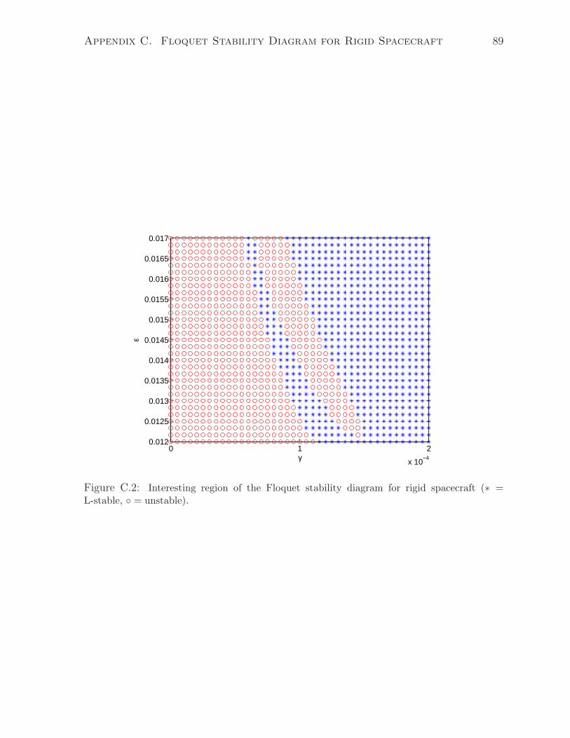
Appendix C. Floquet Stability Diagram for Rigid Spacecraft 89
0 1 2
x 10−4
0.012
0.0125
0.013
0.0135
0.014
0.0145
0.015
0.0155
0.016
0.0165
0.017
γ
ε
Figure C.2: Interesting region of the Floquet stability diagram for rigid spacecraft (∗ =L-stable, = unstable).