
Magdalena Balmaseda, Gianpaolo Balsamo, Roberto Buizza ... · Magdalena Balmaseda, Gianpaolo...
51
656 The new ECMWF seasonal forecast system (System 4) Franco Molteni, Tim Stockdale, Magdalena Balmaseda, Gianpaolo Balsamo, Roberto Buizza, Laura Ferranti, Linus Magnusson, Kristian Mogensen, Tim Palmer and Frederic Vitart Research Department Presented to the SAC 40 th Session 3 – 5 October 2011 November 2011
Transcript of Magdalena Balmaseda, Gianpaolo Balsamo, Roberto Buizza ... · Magdalena Balmaseda, Gianpaolo...

656
The new ECMWF seasonal forecast system (System 4)
Franco Molteni, Tim Stockdale, Magdalena Balmaseda,
Gianpaolo Balsamo, Roberto Buizza, Laura Ferranti, Linus Magnusson,
Kristian Mogensen, Tim Palmer and Frederic Vitart
Research Department
Presented to the SAC 40th Session 3 – 5 October 2011
November 2011

Series: ECMWF Technical Memoranda A full list of ECMWF Publications can be found on our web site under: http://www.ecmwf.int/publications/ Contact: [email protected] © Copyright 2011 European Centre for Medium Range Weather Forecasts Shinfield Park, Reading, Berkshire RG2 9AX, England Literary and scientific copyrights belong to ECMWF and are reserved in all countries. This publication is not to be reprinted or translated in whole or in part without the written permission of the Director. Appropriate non-commercial use will normally be granted under the condition that reference is made to ECMWF. The information within this publication is given in good faith and considered to be true, but ECMWF accepts no liability for error, omission and for loss or damage arising from its use.

The new ECMWF seasonal forecast system (System 4)
Technical Memorandum No.656 1
Abstract
ECMWF will introduce a new seasonal forecast system (System 4) in November 2011 (*), following a line of research and development in extended-range predictions which has spanned almost three decades. The new system is expected to provide advances in the quality of forecast products, feed back onto the ECMWF core activities in terms of atmospheric model diagnostics and ocean modelling/analysis tools, allowing ECMWF to maintain a position of excellence in international programmes and activities on long-range forecasting. This paper illustrates the main methodologies and modelling configurations adopted in the new system, and presents a preliminary assessment of the system performance.
The paper is broadly divided into three parts. The first part describes the configuration of the coupled model, ocean analysis system, and re-forecast set, illustrating the main areas of progress with respect to the current seasonal system (System 3). The second part of the paper deals with “core” results on the coupled model biases and forecast scores for SST and atmospheric variables. It is shown that System 4 delivers improved predictive skill for a majority of parameters and regions, with the additional advantage of a better match between ensemble-mean errors and ensemble spread and therefore increased reliability. This occurs in spite of a cold bias in the tropical Pacific sea surface temperature, which originates from too strong trade winds simulated by the ECMWF atmospheric model in the central and western Pacific. The third part discusses some aspects of System 4 configuration and forecast skill which are worth a more detailed analysis. These include the configuration and scientific results from the new ocean re-analysis (ORA-S4), an assessment of predictive skill for large-scale rainfall anomalies and tropical storm properties, and results of experimentation with momentum flux correction aimed at investigating the impact of IFS tropical wind biases on the coupled system.
In summary, the preliminary assessment of System 4 presented in this paper indicates that System 4 is able to deliver on all major goals that a state-of-the-art seasonal forecast system is expected to attain. As with any new operational system, however, the progress is not uniform, and this highlights the important role of extended-range simulations in providing feedbacks for future improvements in the physical and dynamical aspects of model formulation.
(*) This Memorandum corresponds to the report presented to the ECMWF Scientific Advisory Committee on 3 October 2011. System 4 has actually been implemented operationally on 1 November 2011 and made available to Member States on 8 November 2011.
1. Introduction
ECMWF has been at the forefront of dynamical extended range forecasting since the mid 1980’s, when experimentation on ensemble forecasting for the monthly time scale was started (Molteni et al. 1986, Brankovic et al. 1990). Research on predictability on seasonal time scale in the early 1990’s (eg Palmer and Anderson 1994) led to the implementation of the first ECMWF seasonal forecast system based on a global ocean-atmosphere coupled model in 1997, and a successful forecast of the 1997-98 El Niño (Stockdale et al. 1998). This first coupled system (referred to as System-1) was followed by System-2 in 2001 and the currently operational (at the time of writing) System-3 in March 2007 (Anderson et al. 2007; Stockdale et al. 2011).
The new ECMWF seasonal forecast system (System 4)
2 Technical Memorandum No.656
Since the very beginning, research on extended-range predictability at ECMWF had two main motivations. On the one hand, the potential for providing information about events with strong societal impact was recognised (it is no coincidence that extended-range research was started in 1984, just after the major El Nino of 1982-83 and at the peak of the Sahel drought of the mid eighties). On the other hand, the assessment of the model systematic error which was needed to correct extended-range forecast was seen as an important contribution to the diagnostic work carried out to improve the atmospheric model formulation. These motivations have supported the extended-range forecasting programme of ECMWF throughout its development, and are equally valid today. With regard to the impact on medium-range predictions, it is also worth noting that the efforts on ocean modelling and initialization (initially made in the context of seasonal forecasting) have recently been integrated into the development of the medium-range EPS.
All three ECMWF seasonal forecast systems implemented so far have used the Hamburg Ocean Primitive Equation model (HOPE; Wolff et al 1997) as the ocean component, initialised through an optimum-interpolation (OI) ocean data assimilation scheme which was substantially improved in the transition from System-2 to System-3 (Balmaseda et al. 2008). Although System-3 proved to be a well balanced and skillful system, especially in its predictions of the ENSO phenomenon (Stockdale et al. 2011), the HOPE-OI system was considered obsolete, and it was clear that further progress would have been difficult to achieve until a new ocean model and ocean data assimilation scheme, with potential for future developments, were introduced. At the time of the implementation of System-3, it was agreed that the next-generation system would be based on the NEMO (Nucleus for European Modelling of the Ocean, Madec 2008) ocean model, developed by a consortium of French and British institutions, and a variational ocean data assimilation system (NEMOVAR) developed through a collaboration between ECMWF and research institutes in France and UK (see section 5a).
The new ECMWF seasonal forecast system (System-4), planned to become operational in November 2011, benefits from the transition to the NEMO/NEMOVAR ocean components. Furthermore, progress has been achieved in a number of other areas, including:
The availability of a state-of-the-art re-analysis (ERA-Interim) to provide forcing fluxes for the ocean and initial conditions for the atmosphere;
a recent cycle of the Integrated Forecasting System (IFS) with improved simulation of tropical intra-seasonal variability and reduced biases in the extratropical regions;
higher horizontal and vertical resolution, with a better representation of stratospheric processes and forcings;
a set of re-forecasts spanning a 30-year period with a larger ensemble size than in System-3 (15 vs 11 members);
a larger ensemble size in the operational system (51 vs 41 members), matching the size of the medium-range and monthly ensembles;
a more accurate initialization of land-surface variables;
The new ECMWF seasonal forecast system (System 4)
Technical Memorandum No.656 3
a more sophisticated simulation of model-generated uncertainties, and a simple representation of sea-ice uncertainty through relaxation to alternative sea-ice conditions.
This paper describes the various components of System-4 (S4 hereafter) and presents results about model biases, variability and predictive skill derived from preliminary analyses of the 30-year re-forecast set, making extensive comparisons with System-3 (S3) results.
The paper is broadly divided into three parts. The first part describes the configuration of the coupled model, ocean analysis system, and re-forecast set, illustrating the main areas of progress with respect to the current seasonal system (S3). The second part of the paper deals with “core” results on the coupled model biases and forecast scores for sea surface temperature (SST) and atmospheric variables. It is shown that S4 delivers improved predictive skill for a majority of parameters and regions, with the additional advantage of a better match between ensemble-mean errors and ensemble spread and therefore increased reliability. This occurs in spite of a notable exception to the general reduction of biases in the new system: namely, a cold bias in the tropical Pacific SST which (although partially amplified by ocean-atmosphere coupling) originates from too strong trade winds simulated by the IFS in the central and western Pacific. The third part of the paper discusses in greater depth aspects of System 4 configuration and forecast skill which are worth a more detailed analysis. These include the configuration and selected scientific results from the new ocean re-analysis (ORA-S4), an assessment of predictive skill for large-scale rainfall anomalies and tropical storm properties, and results of experimentation with momentum flux correction aimed at investigating the impact of IFS tropical wind biases on the coupled system. Conclusions and plans for future developments are given in the final section.
2. The seasonal forecast System-4 (S4)
2.1. Ocean model and analysis (NEMO and NEMOVAR)
NEMO (Nucleus for European Modelling of the Ocean, Madec 2008) is a state-of-the-art modelling framework for oceanographic research, operational oceanography, seasonal forecasts and climate studies (for more information see http://www.nemo-ocean.eu/). System 4 uses NEMO version v3.0, with some local modifications (dynamic memory, more flexible output, surface flux forcing, closure of fresh water budget). The grid configuration adopts the ORCA1 grid, which has a horizontal resolution of approx. 1 degree (with equatorial refinement), and 42 levels in the vertical, 18 of which are in the upper 200m. The configuration has been provided by the National Oceanographic Centre (NOC) in Southampton (http://www.noc.soton.ac.uk/nemo/ ). The horizontal resolution is similar to the one used in the current HOPE model, but the resolution in the vertical is increased, especially in the mid-deep ocean (from 29 in HOPE to 42 in NEMO). In the future we refer to the configuration used for S4 as ORCA1_z42.
NEMOVAR is a multi incremental and multivariate variational data assimilation system for the NEMO ocean model. It is based on the variational data assimilation system OPAVAR, and it has been further developed to make it distributed memory (MPI) parallel and consistent with the NEMO structure. It can be used either as a 3Dvar-FGAT system or as a 4Dvar system. The development of NEMOVAR is a collaborative project between ECMWF, the Met Office and CERFACS. It is planned to extend the collaboration to INRIA and the University of Reading.

The new ECMWF seasonal forecast system (System 4)
4 Technical Memorandum No.656
The implementation of NEMOVAR at ECMWF uses the 3DVar-FGAT version. Profiles of temperature and salinity and sea level anomalies from along track altimeter are assimilated in a 10-day assimilation cycle. Multivariate relationships are imposed between temperature, salinity and sea level in order to preserve the vertical water mass properties, preserving hydrostatic and geostrophic balance. The first guess is produced by integrating forward the NEMO model forced by daily fluxes, relaxed to SST and bias corrected. The model equivalent of each available observation is calculated, and a quality control of the observations performed. In the final phase of the analysis cycle, the assimilation increment resulting from the inner loop is applied using the incremental analysis update (IAU, Bloom et al 1996), during a second model integration spanning the same window as that used to provide the first guess.
There are two ocean analysis streams: the reanalysis stream (ORA-S4), used to provide initial conditions for the calibrating hindcasts, which runs behind real time, and the real-time stream, an early delivery ocean analysis suite that produces timely initial conditions for the EPS and seasonal real time forecasts. Further information on the NEMOVAR analysis, and specifically on the ocean reanalysis performed with this system, are given in section 5.1
2.2. Atmospheric model
2.2.1. Model configuration
The atmospheric component of the S4 forecast system is the IFS Cycle 36r4. This model version was introduced for operational medium-range forecasting on the 9th of November 2010, at the time when System 4 configuration was being finalised. Earlier versions of the model (e.g. cycle 36r1) had shown larger bias and less skilful ENSO forecasts than 36r4. The possibility to use model cycle 37r2, which was under final testing and due to replace 36r4, was considered, but delaying implementation of S4 in order to adopt this cycle was ruled out, since experimentation showed a slight degradation in performance. The adoption of even later cycles would have caused substantial delay in the introduction of S4, and was not considered a viable option.
Care was taken to define a cost-effective configuration that would provide users with a large enough hindcast dataset, a larger ensemble size, and a better, higher-resolution coupled system. The key differences between S3 and S4 in the IFS and ensemble configurations are listed in Table 2.2.1., while Appendix B provides a comparison with extended-range forecast systems at other institutions worldwide.
IFS cycle
IFS Hor Res
IFS Vert Res
IFS model unc.
Ensemble members (length)
Re-forecast years
Re-forecast members
S3 31r1 TL159 L62 Top: 5 hPa
1-lev SPPT 41 (0÷7m) 11 (7÷13m)
25 1981-2005
11 (0÷7m) 5 (7÷13m)
S4 36r4 TL255 L91 Top .01 hPa
3-lev SPPT and SPBS
51 (0÷7m) 15 (7÷13m)
30 1981-2010
15 (0÷7m) 15 (7÷13m)
Table 2.2.1. Key differences between the IFS and ensemble settings in the operational system-3 (S3) and the forthcoming S4.

The new ECMWF seasonal forecast system (System 4)
Technical Memorandum No.656 5
Suitable choices have been made for both horizontal and vertical resolution, considering both performance and affordability. We use the 91 level version, with a model top in the mesosphere at 0.01 hPa, or a height of approximately 74 km. This is primarily to allow a better representation of the stratosphere, given multiple indications that stratospheric processes can impact seasonal forecasts (Shindell et al 2004; Cagnozzo and Manzini 2009; Marshall and Scaife, 2009) and early experiments demonstrating particular sensitivity in the European region to stratospheric perturbations. Given that predictability is often low in the European region, it is important to consider any possible source of predictable signals. The rationale for including a better stratosphere at this stage was not so much with the expectation of an immediate increase in skill, but to lay a foundation on which future development can take place. Still, early testing in research mode indicated detectable benefits of vertical resolution to tropospheric and NH seasonal scores, which encouraged the introduction of 91 levels even at this stage of development.
The horizontal resolution is increased from TL159 to TL255. The grid point calculations are on the corresponding reduced N128 gaussian grid, which has about a 0.7 degrees spacing. The time step is 45 minutes. The increase in horizontal resolution is the most expensive single part of the upgrade from S3 to S4 as far as the operational runs are concerned. It gives clear and substantial improvements in the model climate, which is very desirable for a seasonal forecast system. There is very little impact on ENSO, however. The impact on tropospheric scores is positive on average, but the impact appears to be weaker than that of the vertical resolution upgrade.
The use of a more recent cycle of the IFS (containing more advanced physical parametrizations than 4 years ago) and the increase in horizontal and vertical resolution make the new system more expensive than the old one when running on the same computer. The NEMO ocean model can run more efficiently than HOPE, although at these resolutions the ocean is only a small part of the cost of the coupled model. More importantly, the cost of the coupled system is influenced by associated technical changes (NEMO allows the IFS to run in pure MPI mode, which is significantly more efficient than the pure openMP mode required by HOPE, and the use of the OASIS3 interface gives more efficient coupling), such that the coupled system now runs more efficiently than before. The net result is that despite the resolution increases, the S4 model is about 24% cheaper to run relative to available computer resources than was the S3 model.
IFS model cycle 36r4 is used with a few modifications. The new FLAKE lake model (Balsamo et al. 2011) is activated to provide temperature and ice data for resolved lakes, but is run only in climatological mode since the prognostic version of the code was not fully available in time. This development was necessary because the S3 treatment of lakes (also based on estimated climatological values, but in a more ad-hoc way) was not transferable to S4 for technical reasons. The default OASIS3 treatment of lakes is to interpolate from the nearest ocean points, which can give poor results, and the use of FLAKE in climatological mode is a big improvement on this.
Some adjustments have been made to stratospheric physics. The overall amplitude of the non-orographic gravity wave drag is reduced, to give a better evolution of the QBO and a better stratospheric climate. A higher level of non-orographic wave drag is imposed at high southern latitudes, which partially compensates for numerical damping of highly active resolved gravity waves at these latitudes. The non-conserving action of a gravity wave drag limiter is reduced to improve the realism of the model physics. Ozone is activated as a prognostic variable, and unlike the medium-

The new ECMWF seasonal forecast system (System 4)
6 Technical Memorandum No.656
range forecasts, ozone is radiatively active. As in S3, we specify time-variation of greenhouse gases to improve the simulation of trends during the re-forecast period. We also specify a time-varying solar cycle, including an extrapolation into the future (following recommendations for IPCC AR5). The variation is not spectrally resolved, however, and so the impact of UV variations on the stratosphere is missing from our model. Volcanic aerosols are included based on the estimated distribution in the month prior to the start of the forecast, and then follow a damped persistence. A more complete description of the treatment of volcanic aerosols and the stratosphere is given in Appendix A.
Although a dynamical sea-ice model is not yet included in the coupled system, the specification of sea-ice conditions has been improved. In S3 a long-term sea-ice climatology was specified, but this is no longer tenable for real-time forecasts, given the large reductions in Arctic sea-ice extent in recent years. In the S4 forecast for a given year, we specify sea-ice by sampling from the previous 5 years. This both captures the main part of the trend in sea-ice, and also gives a representation of the uncertainty in sea-ice conditions. It also means that all integrations use a realistic ice field that contains appropriately sharp boundaries to the sea-ice (rather than a smoothly varying multi-year mean). As in S3, sea-ice for the first 10 days of the forecast persists the initial sea-ice analysis; then over the next 20 days there is a transition towards the specified ice conditions derived from the previous 5 years.
The atmosphere and ocean are coupled using a version of the OASIS3 coupler developed at CERFACS. This is used to interpolate between oceanic and atmospheric grids with a coupling interval of 3 hours, which allows some resolution of the diurnal cycle. A gaussian method is used for interpolation in both directions, primarily due to the complexity of the ORCA1 grid. The gaussian method automatically accounts for the inevitably different coastlines of the two models - values at land points are never used in the coupling, since these can be physically very different to conditions
over water.
2.2.2. Simulation of model uncertainties
S4 uses two stochastic schemes, both the 3-time level SPPT scheme (SPPT3) and the stochastic backscatter scheme (SKEB) (see Palmer et al. 2009). The SPPT3 and SKEB settings are identical to those used in the medium-range EPS – indeed the choices for SPPT3 made in the EPS were informed by experimentation with the seasonal forecast system, aimed at identifying an amplitude for the longer timescale perturbations that would be suitable for use both in medium and seasonal range integrations. Note that the SPPT3 scheme in particular is efficient at exciting a divergence in the ENSO SSTs of the coupled model forecast - the spread in ENSO forecasts from System 4 is substantially larger than in System 3.
With the current configuration of stochastic schemes, the SKEB scheme has little impact on the seasonal forecasts at T255 resolution, and only a very slight impact on the model climate. Testing of the impact of the stochastic schemes highlighted the difficulty of affording large enough sample sizes to make definitive statements about the impact of minor changes on the performance of a seasonal forecast system, particularly as regards its mid-latitude performance. Changes with large benefits can be assessed at low cost; a change with possible small benefit is more expensive to characterise, and uncertainties are likely to remain about the actual impact.

The new ECMWF seasonal forecast system (System 4)
Technical Memorandum No.656 7
2.3. Initial conditions for the coupled system
2.3.1. Unperturbed (control) initial conditions
The atmospheric unperturbed (i.e. for the control forecast) initial conditions come from ERA Interim for the period 1981 to 2010 and from ECMWF operational analysis from 1st January 2011 onwards, since ERA Interim is not available for use in real-time. Although this risks introducing some inconsistency between the re-forecasts and the real-time forecasts, the problem is controlled by using special treatment for sensitive fields, namely land surface fields and ozone. The treatment of land surface initial conditions is discussed in Appendix A: re-forecasts use the output of an offline run of the land surface model, and the forecasts use the operational land surface analysis subject to certain adjustments and constraints.
Since the model has radiatively interactive ozone, it needs ozone initial conditions. Unfortunately the interannual variability of ozone in ERA interim is significantly affected by changes in satellite instruments. Since these changes were found to drive spurious temperature variations in the stratosphere, it was decided not to use the time-dependent ERA interim ozone as initial conditions. Instead, a seasonally varying climatology is formed from what are believed to be the most reliable years of the ERA interim ozone analyses (1996-2002), and the ozone initial conditions are taken from this climatology. Although we do not provide any initial data on ozone anomalies, the ozone field is free to develop during the forecast and will develop anomalies physically consistent with e.g. temperature anomalies and specified CFC time history / projection. The use of interactive ozone with climatological initial conditions is of some benefit to the stratospheric forecasts, but clearly if adequate ozone analyses were available, more benefit could be extracted.
Ocean initial conditions come from ORA-S4 for the re-forecast period, and from the real-time NEMOVAR for the operational runs (see Sect. 2.1 and 5.1).
2.3.2. Perturbed initial conditions
The ensembles for each forecast or re-forecast are generated by using an ensemble of initial conditions and by the use of stochastic physics. At the seasonal timescale, most of the spread in the ensemble is internally generated (with or without the help of stochastic physics), so the role of initial perturbations is limited. Nonetheless, we attempt a good representation of the most important perturbations, to allow a realistic evolution of ensemble spread through the early part of the forecast.
The ocean analyses are provided as a 5 member ensemble. The ensemble of analyses is driven by sampling uncertainty in winds and in deep ocean initial conditions, and sub-sampling observation coverage. The ocean analyses are then augmented by applying SST perturbations (as many as needed), with an associated sub-surface temperature signal. The ocean initial conditions thus represent the main uncertainties in the ocean state. For the atmosphere, the operational EPS machinery is used to calculate singular vectors and targeted singular sectors in the tropics, using 36r4 operational settings. Since EDA output is not available for use by the re-forecasts, EDA is not used. Evolved singular vectors are not calculated either. The perturbations applied to the upper air fields are thus somewhat simplified compared to the full EPS system. They nonetheless allow a reasonably accurate growth of Z500 spread over the first 10 days of the forecast, and are appropriate for the needs of the seasonal

The new ECMWF seasonal forecast system (System 4)
8 Technical Memorandum No.656
forecast system. Perturbations are not applied to the land surface initial conditions; this is planned to be addressed in further development of the land surface initialization system.
2.4. Re-forecasts
Every seasonal forecast model suffers from bias - the climate of the model forecasts differs to a greater or lesser extent from the observed climate. Since variations in the predicted seasonal distributions are often small, this bias needs to be taken into account, and must be estimated from a previous set of model integrations. Also, it is vital that users know the skill of a seasonal forecasting system if they are to make proper use of it, and again this requires a set of forecasts from earlier dates.
The re-forecasts (also referred to as hindcasts) for S4 are made starting on the 1st of every month for the years 1981-2010. The ensemble size is 15 members (increased from 11 in S3 to provide more reliable statistics). The data from these forecasts is available to users of the real-time forecast data, to allow them to calibrate their own real-time forecast products. Once S4 is operational, it is planned to run additional re-forecast ensemble members for a sub-set of dates, to allow a better sampled characterization of skill. This is particularly important for regions and times when the forcing signal is low – a large ensemble size is needed to avoid spurious “signals” due to inadequate sampling.
2.5. Operational forecasts
The seasonal forecasts consist of a 51 member ensemble, as in the medium-range and monthly EPS. The ensemble is constructed by combining the 5-member ensemble ocean analysis with SST perturbations and the activation of stochastic physics. The forecasts have an initial date of the 1st of each month, and run for 7 months. Forecast data and products are released at 12Z UTC on a specific day of the month. For System 4, this is expected to be the 8th.
In addition to the seasonal forecast which is made every month, an annual-range forecast is made four times per year, with start dates the 1st February, 1st May, 1st August and 1st November. The range of the forecast is 13 months. The annual range forecasts are run as an extension of the seasonal forecasts, and are made using the same model but with a smaller ensemble size. Both re-forecasts and real-time forecasts and have an ensemble size of 15. The annual range forecasts are designed primarily to give an outlook for El Nino. At present they have an experimental rather than operational status.
3. Systematic errors in System 4
3.1. Global patterns of model biases
The quality of a seasonal prediction system is ultimately measured by the quality of its forecasts. However, the verisimilitude of the model’s mean state is a necessary test of its quality, which is relevant both to the likely performance in forecast mode and to understanding any issues and problems regarding the model formulation. A particular advantage of looking at model climate is that, by integrating data over the whole range of the re-forecast set, it is much better sampled than time-dependent properties, e.g. mid-latitude forecast scores. For the sake of brevity, in this section we only highlight a few features of the model mean state, focussing on the 2-to-4-month forecast range.
The first assessment is for the SST, since this is possibly the most critical field defining the state of the coupled ocean atmosphere system. Figure3.1.1 shows SST bias from the early range of the forecasts

The new ECMWF seasonal forecast system (System 4)
Technical Memorandum No.656 9
verifying in DJF for S4 and S3. Several features can be highlighted: S4 has a better annual cycle of SST at higher latitudes and in particular a reduced warm bias in the Southern Ocean. On the other hand, S4 has a more pronounced “cold tongue” bias in the equatorial Pacific (see section 3.2). Further analysis (not shown) shows that S4 has a much improved seasonal cycle in the far eastern Pacific and in the equatorial Atlantic.
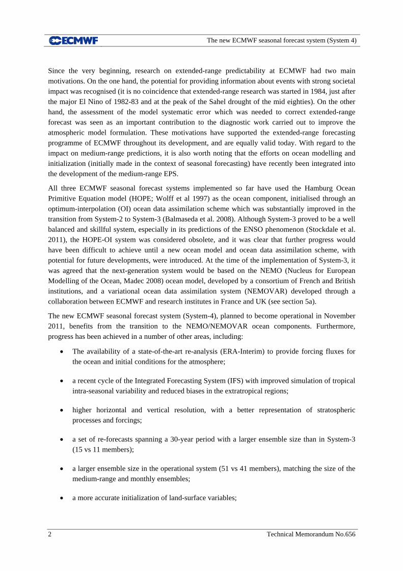
The improvements in physical parametrizations introduced between cycles 31r1 (S3) and 36r4 (S4) have a stronger impact on the reduction of biases when looking at purely atmospheric fields. To provide just two examples, Figures 3.1.2 and 3.1.3 show biases in DJF MSLP and JJA T850, respectively. The MSLP field in boreal winter is much improved in S4, which is indicative of a more accurate zonal-mean circulation as well as better amplitude and phase of planetary waves. Big improvements are visible in surface and upper air wind fields, and in geopotential height fields (not shown). For the T850 fields, the reduced bias in the SH winter is the most apparent feature, but note also the reduction of the cold bias over Canada and Siberia. Stratosphere biases are also dramatically reduced in S4 (not shown).
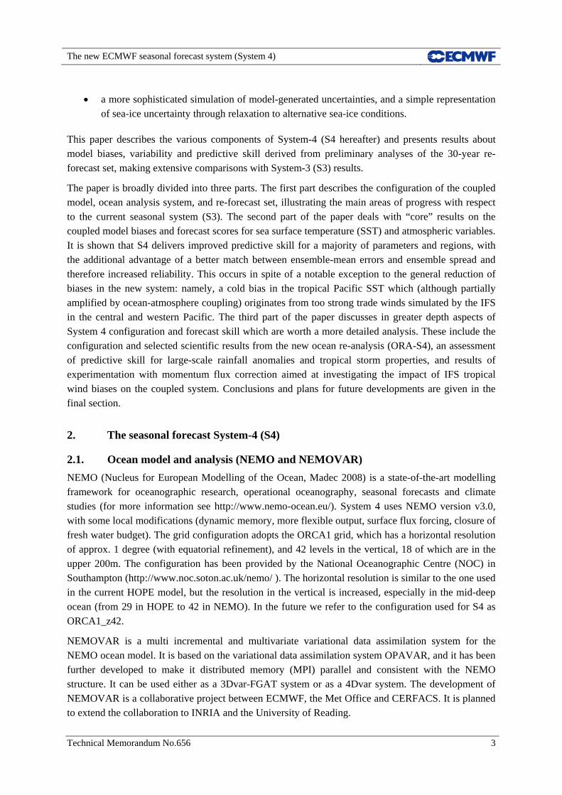
Finally, we show in Figure 3.1.4 the precipitation bias for JJA, relative to Global Precipitation Climatology Project data (GPCP v2.1). There are some important reductions in bias, particularly in the tropical Atlantic and Indian Oceans, and some improvements over land areas e.g. in East Asia and over the Amazon basin. However, there are clearly significant biases remaining in many areas, even allowing for imperfections in the verification data: particularly evident is the excess of rainfall over most of Indonesia and the Philippines.

The new ECMWF seasonal forecast system (System 4)
10 Technical Memorandum No.656
Figure 3.1.1: SST bias in DJF (from November start dates), for S4 (top) and S3 (bottom).
Figure 3.1.2: DJF MSLP bias in DJF (from November start dates), for S4 (top) and S3 (bottom)
The new ECMWF seasonal forecast system (System 4)
Technical Memorandum No.656 11
Figure 3.1.3: T850 bias in JJA (from May start dates), for S4 (top) and S3 (bottom)
Figure 3.1.4: Precipitation bias in JJA (from May) with respect to GPCP: S4 (top), S3 (bottom).
The new ECMWF seasonal forecast system (System 4)
12 Technical Memorandum No.656
3.2. Biases affecting the ENSO evolution
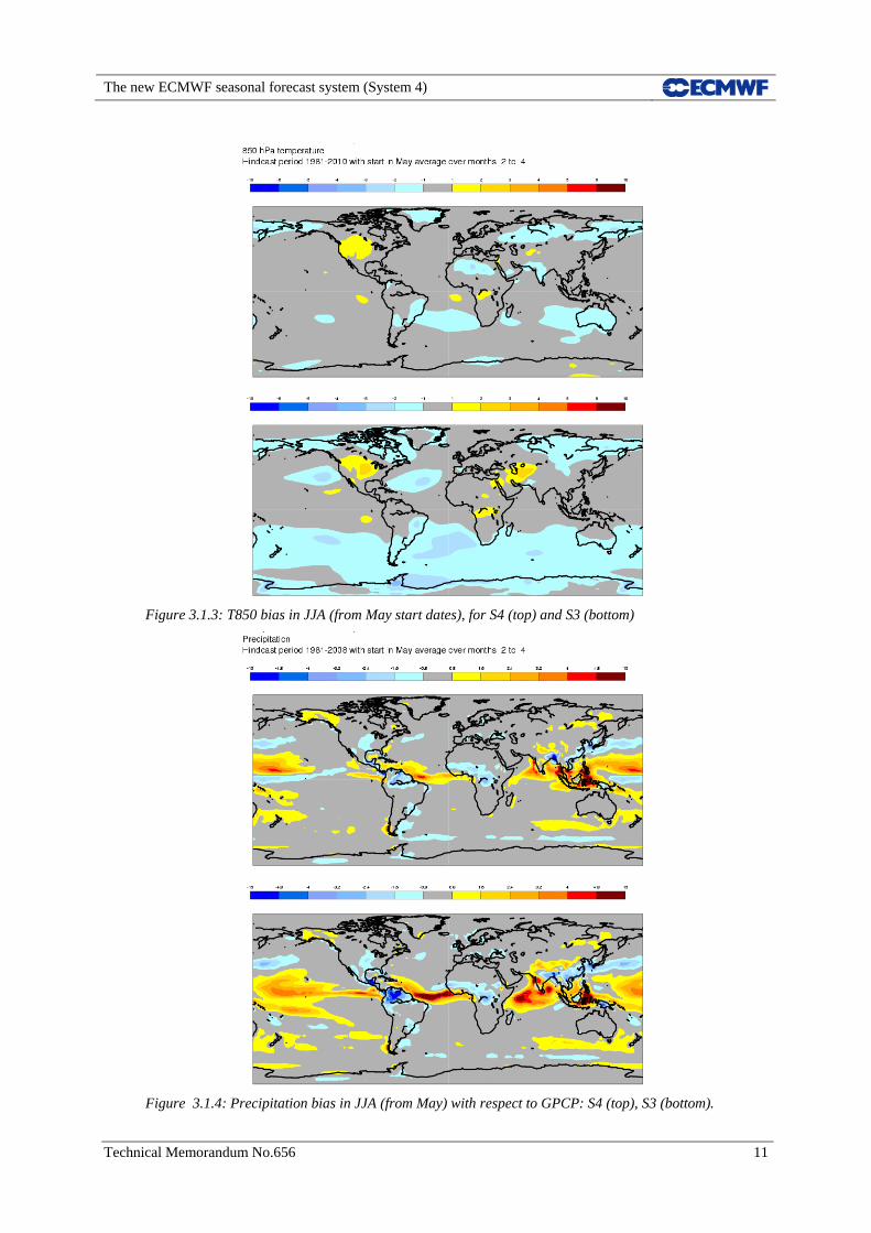
Although (as seen above) large reductions in model bias are present in many areas, S4 suffers from one problem that is particularly relevant to seasonal variability: a bias in the near-equatorial winds in the west and central Pacific. This wind bias is the dominant factor in driving an SST bias in the coupled model, whereby equatorial SSTs in the Pacific drift to cold conditions. Figure 3.2.1 compares the SST drift in the central Pacific for S3 and S4, in the Nino 3.4 region. Although the wind bias, which is also seen in runs of the IFS with observed SST, is the dominant cause, comparisons with HOPE suggest that a part of the SST bias may be related to the ocean model. Higher resolution in the ocean model might help alleviate this part of the problem in future implementations of the seasonal forecast system.
Figure 3.2.1: Mean SST evolution in Nino3.4 from System 4 (red) and System 3 (blue)
A cold bias of this magnitude was also seen in the very first ECMWF seasonal forecasting system, and is not necessarily an insurmountable obstacle to ENSO forecasts. The bias was actually stronger in IFS versions preceding cycle 36r4 (for example in cycle 36r1), where it was large enough to have a serious impact on SST forecast skill. For that reason, investigation was made of possible flux correction techniques to ameliorate the problem, as discussed in Section 5.4. These experiments clarified that there are two main impacts of this sort of mean error: a loss in skill in the west Pacific (especially the cold-tongue/warm pool boundary), and a high sensitivity of the amplitude of SST variability in the East Pacific to the mean state error. The anomaly correlation (ACC) of east Pacific variables is relatively unaffected. Improvements in the IFS made in cycle 36r4 meant that the skill problems were sufficiently reduced that the benefits of flux correction were no longer overwhelming, when ACC was assessed. Therefore, it was felt that there was insufficient motivation to introduce an empirical correction term into the S4 coupled model, which would make the assessment of future progress in model physics more difficult to assess on the seasonal scale. On the other hand, we are aware that this bias has a progressively larger impact on long lead times (~ 1year) and on parameters which are strongly sensitive to the mean SST (see further discussion in section 5.4).
However, a problem still present with cycle 36r4 is a significant over-estimation of SST amplitude in the east Pacific (see Figure 3.2.2). The over estimation is seasonally varying, and reaches its maximum for lead times of a few months verifying during the boreal spring. For the purpose of producing forecasts of “Nino SST” indices (one of the major seasonal forecast products), it is suggested to scale the forecast anomalies appropriately. While the mean of the SST forecasts is already corrected by the
0 1 2 3 4 5 6 7 8 9 10 11 12 13 14 15 16 17 18Calendar month
23
24
25
26
27
28
29
Ab
solu
te S
ST
NINO3.4 mean absolute SST

The new ECMWF seasonal forecast system (System 4)
Technical Memorandum No.656 13
process of bias removal, the proposed approach involves the additional step of correcting the variance of the model output to match the observed variance. (As with other skill assessment, this is done in cross-validated mode for the re-forecast period, which decreases the calculated scores slightly). Note that this technique is not the same as optimizing the amplitude of the forecasts to give the best rms error, which might give the best re-forecast statistics but risks damping forecast anomalies unphysically towards zero if the forecast performance is poor.
Figure 3.2.2 demonstrates the impact of such a variance correction. The uncorrected S4 forecasts are appreciably worse than S3 in terms of mean-square skill score (MSSS), and have a large overestimation of amplitude. The corrected S4 forecasts have much higher skill than S3. Note that because S3 is underactive, re-scaling the amplitude typically does not help the MSSS – in most cases, it makes it worse. The reason why this re-scaling is so successful is that S4 has a very high ACC skill in the east Pacific.
Comparisons of flux-corrected SST forecasts with variance-scaled, non-flux-corrected SST forecasts show that the variance re-scaling removes the advantage of the flux correction as far as SST scores are concerned. For east Pacific SST products, flux correction has no substantial benefit. Of course there is a very important difference between a flux-corrected forecast and a forecast which is variance scaled at the plot stage: the SST anomaly seen by the atmosphere in the non-flux corrected case is too big. However, diagnostics show that the atmospheric response to a 1 deg SST anomaly in S4 typically has a realistic spatial structure, but the amplitude is too weak (see end of Sect. 5.2) – that is, for S4 the amplitude of SST teleconnections are more realistic if the SST anomalies are larger than observed. In other words, the effect of too large ENSO SST anomalies is compensated to a large extent by a reduced sensitivity to those SST anomalies.
Figure3.2.3 shows an example of a variance-corrected forecast from S4, made at the time of year when the scaling is strongest, and how the corresponding SST plume is much more realistic when the correction is made.
Figure3.2.2: NINO3 statistics in S4 with (red) and without (blue) variance correction and S3 (green). Left: mean-square skill score; right: anomaly amplitude w.r.t. observations.
0 1 2 3 4 5 6 7Forecast time (months)
0
0.2
0.4
0.6
0.8
1
Me
an
sq
ua
re s
kill
sco
re
Ensemble sizes are 15 (0001), 11 (0001) and 11 (0001)150 start dates from 19910201 to 20081101, various corrections
NINO3 SST mean square skill scores
Fcast S4 Fcast S4 Fcast S3 Persistence
0 1 2 3 4 5 6 7Forecast time (months)
0.4
0.6
0.8
1
1.2
1.4
1.6
Am
plit
ud
e R
atio
NINO3 SST anomaly amplitude ratio

The new ECMWF seasonal forecast system (System 4)
14 Technical Memorandum No.656
Figure 3.2.3 NINO3 plume from forecasts started on 1 Nov 1997: S4 with (red) and without (blue) variance correction and S3 (green).
4. System-4 skill scores
4.1. ENSO and other SST scores
We present here ENSO and other SST statistics based on the full set of re-forecasts for S4 (1981-2010), unless otherwise stated. Comparisons with other forecasts are always for a common set of dates. The S4 re-forecasts are corrected (in cross-validated mode) for both mean and variance, whereas the S3 forecasts are corrected only for mean, since we want to compare the end-to-end forecasting systems. (In most cases, correcting S3 for variance makes the S3 scores worse, so uniform processing of the data would only exaggerate the performance gains of S4.) Re-forecasts for S4 consist of 15 members, while only 11 members are available for S3. This might seem an unfair advantage for S4, but S4 has much larger ensemble spread than S3, and the extra ensemble members compensate for the additional “noise” in the ensemble mean. It is possible to adjust the RMSE scores for both systems to the score expected for an arbitrarily large ensemble (which approximates the real-time forecast situation – a 41 or 51 member ensemble has only modest uncertainty in its mean). When this is done, the relative performance of S4 versus S3 looks consistent with the one obtained from non-adjusted scores; therefore, to keep things simple, we show the scores without ensemble-size adjustment.
In NINO4 (Figure 4.1.2, left), the SST forecast skill is marginally worse than S3. Most of this deterioration in fact stems from a single event, the 1997 El Nino, where the S4 model gives unphysically large SST anomalies. Similar behaviour has been seen in other ENSO forecast models for this event. The fundamental cause is a lack of linearity, as the upwelling of cold water switches off and the cold bias in the model is strongly reduced: the model absolute SST is in fact very realistic, but the anomaly relative to the usual cold bias is much too warm. This behaviour is clearly related to the
MAY2007
JUN JUL AUG SEP OCT NOV DEC JAN2008
FEB MAR APR MAY JUN JUL
-3
-2
-1
0
1
Ano
mal
y (d
eg C
)
-3
-2
-1
0
1
Monthly mean anomalies relative to NCEP adjusted OIv2 1971-2000 climatologyECMWF forecasts from 1 Nov 2007
NINO3 SST anomaly plume
System 4System 4System 3

The new ECMWF seasonal forecast system (System 4)
Technical Memorandum No.656 15
significant model bias in the tropical Pacific, which hopefully will be reduced in future versions. Operationally, the impact of a similar kind of error on real-time forecasts of El Nino SST indices is likely to be mitigated by a proper physical interpretation of the model output. However, this also means the teleconnections for the 1997 event or future large events might be affected, which is harder to account for when interpreting the model output.
The right-hand panels in Figure 4.1.2 show the forecasts in the equatorial Atlantic (EQATL), where S4 gives strong improvements over S3, and now provides forecasts which are substantially better than persistence or climatology. Note also the near perfect match between spread and error. These improvements are at least partly related to a much improved mean state in this region, together with an improvement in the ocean analyses. Other tropical Atlantic regions also show noticeable improvements in skill, as do other regions such as the North Pacific and Indian Ocean – indeed, S4 beats S3 almost everywhere. The improved spread/skill comparison is also very widespread. The west Pacific (including the NINO4 and western equatorial Pacific EQ3 areas) is the only region where S4 performance disappoints in comparison with S3, and where there is still a major mis-match between ensemble spread and rms forecast error. This is due to the specific errors stemming from model bias (eg the 1997 case discussed above), which would be improper to represent by adding stochastic noise to the ensemble.
As with S3, S4 shows an overall reduction in NINO3 and NINO3.4 SST errors over time, with errors in the post-TAO era (1994 onwards) being lower than the pre-TAO era (figures not shown). The Atlantic also shows better skill in the more recent period. Some variation can occur due to sampling of different periods with different variability characteristics, but this is unlikely to be the dominant cause of the improvements, certainly in the Pacific (Stockdale et al, 2011). Although the ENSO ensemble forecasts are slightly under-dispersive (spread is less than error) for the 30 year hindcast period as a whole, the result for the 17 years of the post-TAO era is different: here S4 is modestly over-dispersive at longer leads in NINO3, while being only modestly under-dispersive in NINO3.4. The matching of the stochastic physics amplitude to the observed forecast error statistics is thus judged to be about right for the real-time forecast system, for which the more recent past gives a better guide to expected forecast error.
As well as the main seasonal forecasts, both S3 and S4 include a small number of “annual range” forecasts. These are made only once per quarter, extend for 13 months, and are intended to give an outlook for ENSO, which still has significant predictability at these longer timescales. Plots of rms error (not shown) suggest that at lead times beyond 7 months, S4 performs somewhat less well than S3 in the main El Nino regions. Estimates of the score sampling error, however, indicate that this result may not be reliable due to the large scatter of scores in individual cases and ensemble size limitations. To illustrate the impact of event sampling on the scores, Figure 4.1.3 shows a scatter diagram, where each point represents a given forecast date, and the Mean Absolute Error (MAE) of S3 and S4 for that date, for the months 8-13. A point below the line is a case where S3 is a better forecast; a point above the line is a case where S4 is better. Consistent with the RMSE analysis, S3 is ahead on average; but the scatter diagram makes clear that there is a wide spread, and the under-performance of S4 is not statistically significant.

The new ECMWF seasonal forecast system (System 4)
16 Technical Memorandum No.656
Figure4.1.1. S4 (red) and S3 (blue) NINO3 and NINO3.4 SST scores for the 30 year re-forecast period. S4 has decreased error (solid line) and increased ensemble spread (dashed line).
Figure4.1.2. As above, but for NINO4 and Equatorial Atlantic SST.
0 1 2 3 4 5 6 7Forecast time (months)
0.4
0.5
0.6
0.7
0.8
0.9
1
An
om
aly
co
rre
latio
n
wrt NCEP adjusted OIv2 1971-2000 climatology
NINO3 SST anomaly correlation
0 1 2 3 4 5 6 7Forecast time (months)
0
0.2
0.4
0.6
0.8
1
1.2
Rm
s e
rro
r (d
eg
C)
95% confidence interval for 0001, for given set of start datesEnsemble sizes/corrections are 15/AS (0001) and 11/BC (0001)360 start dates from 19810101 to 20101201, various corrections
NINO3 SST rms errors
Fcast S4 Fcast S3 Persistence Ensemble sd
0 1 2 3 4 5 6 7Forecast time (months)
0.4
0.5
0.6
0.7
0.8
0.9
1
An
om
aly
co
rre
latio
n
wrt NCEP adjusted OIv2 1971-2000 climatology
NINO3.4 SST anomaly correlation
0 1 2 3 4 5 6 7Forecast time (months)
0
0.2
0.4
0.6
0.8
1
Rm
s e
rro
r (d
eg
C)
95% confidence interval for 0001, for given set of start datesEnsemble sizes/corrections are 15/AS (0001) and 11/BC (0001)360 start dates from 19810101 to 20101201, various corrections
NINO3.4 SST rms errors
Fcast S4 Fcast S3 Persistence Ensemble sd
0 1 2 3 4 5 6 7Forecast time (months)
0.4
0.5
0.6
0.7
0.8
0.9
1
An
om
aly
co
rre
latio
n
wrt NCEP adjusted OIv2 1971-2000 climatology
NINO4 SST anomaly correlation
0 1 2 3 4 5 6 7Forecast time (months)
0
0.2
0.4
0.6
0.8
Rm
s e
rro
r (d
eg
C)
95% confidence interval for 0001, for given set of start datesEnsemble sizes/corrections are 15/AS (0001) and 11/BC (0001)360 start dates from 19810101 to 20101201, various corrections
NINO4 SST rms errors
Fcast S4 Fcast S3 Persistence Ensemble sd
0 1 2 3 4 5 6 7Forecast time (months)
0.4
0.5
0.6
0.7
0.8
0.9
1
An
om
aly
co
rre
latio
n
wrt NCEP adjusted OIv2 1971-2000 climatology
EQATL SST anomaly correlation
0 1 2 3 4 5 6 7Forecast time (months)
0
0.2
0.4
0.6
Rm
s e
rro
r (d
eg
C)
95% confidence interval for 0001, for given set of start datesEnsemble sizes/corrections are 15/AS (0001) and 11/BC (0001)360 start dates from 19810101 to 20101201, various corrections
EQATL SST rms errors
Fcast S4 Fcast S3 Persistence Ensemble sd

The new ECMWF seasonal forecast system (System 4)
Technical Memorandum No.656 17
Figure4.1.3: Scatter plot of Mean Absolute Error from months 8-13 of the annual range NINO3.4 SST forecasts, comparing S4 and S3 for the 118 cases which can be verified. S3 provides the best forecast slightly more often than S4, but the difference is not significant.
Although the mean state errors are having some negative effect on the S4 forecasts at longer leads, the annual range forecasts continue to have a substantial level of skill at predicting ENSO SST out to 13 months. Some consideration was given to running the annual range part of the forecast system using flux correction, but preliminary tests showed limited benefits (mainly in the west Pacific in the earlier forecast range), which did not justify the additional complexity.
Scores so far have been compared with the present operational system, S3. A sense of the longer term progress in our forecast systems can be obtained by including our earlier systems (S1 and S2) in the comparison. Since these systems were run for a shorter period of time (and in particular are missing the most recent and well-observed years), comparisons may be less accurate than those we can make between S3 and S4 alone. Table 4.1.1 shows the aggregate MAE scores for months 1-6 for the common period 1987-2002 for the four systems, for several El Nino regions, and for the “Figure of merit (FOM)” that has been often used to produce a summary score for an ENSO forecasting system, and which is obtained as the sum of the NINO3, NINO3.4 and NINO4 values.
System NINO1+2 NINO3 NINO3.4 NINO4 EQ3 FOM
S1 (16y) 0.642 0.454 0.430 0.283 0.258 1167
S2 (16y) 0.620 0.406 0.391 0.319 0.250 1116
S3 (16y) 0.593 0.373 0.332 0.261 0.223 966
S4 (16y) 0.493 0.329 0.330 0.280 0.228 939
S3 (30y) 0.574 0.363 0.315 0.250 0.216 928
S4 (30y) 0.501 0.324 0.296 0.257 0.227 877
Table 4.1.1 Tropical Pacific MAE scores for different ECMWF seasonal forecast systems. Best values in the two considered periods (1987-2002) and (1981-2010) are in bold.
0 0.2 0.4 0.6 0.8 1 1.2 1.4 1.6 1.8 2MAE of S4/m3
0
0.2
0.4
0.6
0.8
1
1.2
1.4
1.6
1.8
2
MA
E o
f S
3/m
3
Ensemble sizes are 5 (S3/m3) and 15 (S4/m3)118 start dates from 19810201 to 20100501
NINO3.4 SST error comparison
S4/m3 wins 54 timesS3/m3 wins 64 times
range: 8-13 months

The new ECMWF seasonal forecast system (System 4)
18 Technical Memorandum No.656
The table shows that the improvement in the East Pacific (NINO3 and especially NINO1+2) is quite large compared to previous improvements, whereas following the very large improvement in NINO3.4 seen in S3, only very modest additional improvement is made. Performance in NINO4 has not been monotonic – S2 was a lot worse than S1, then S3 gave a big improvement, while S4 has gone back slightly. Previous studies (Anderson et al, 2007) have shown that the NINO4 region is the most sensitive to the mean state. It is the one area where we could have obtained significantly better scores if we had used flux correction (see Section 5.4).
We also show the same statistics calculated from S3 and S4 for the full 30 year period. The overall picture is similar to the reduced 16 year period as regards the spatial distribution of improvement/deterioration, but the overall improvement comes out higher, notably in NINO3.4.
For a final perspective, we show the performance of S4 and S3 against the other EUROSIP models, from the Met Office and Météo-France. The Met Office now calculates their re-forecasts only in near-real time. We use their most recent version for which a year of data exists, which is the version that ran from late 2009 to almost the end of 2010. For this version, the re-forecast period available covers the 14 years 1989-2002. Re-forecast data is available for 11 months, and Figure4.1.4 shows MSSS (Mean Square Skill Score against climatology) in the three main El Nino regions for S4, S3 and the other European models for these dates. Since the Met Office model has a similar over-activity to S4, it is processed in the same way (ie with variance scaling), which improves the MSSS. The Meteo-France and S3 models are underactive, and do not have their variance scaled.
Figure4.1.4 . MSSS for S4 (red), S3 (blue), Meteo-France (green) and Met Office (orange), for the years 1989-2002, for NINO3, NINO3.4 and NINO4. Scores for persistence are in black.
0 1 2 3 4 5 6Forecast time (months)
0
0.2
0.4
0.6
0.8
1
Mean s
quare
ski
ll sc
ore
Ensemble sizes are 15 (0001), 11 (0001), 11 (0001) and 11 (0001)154 start dates from 19890201 to 20021201, various corrections
NINO3 SST mean square skill scores
ECMWF S4 ECMWF S3 Météo-France S3 Met Office S4
0 1 2 3 4 5 6Forecast time (months)
0
0.2
0.4
0.6
0.8
1
Mean s
quare
ski
ll sc
ore
Ensemble sizes are 15 (0001), 11 (0001), 11 (0001) and 11 (0001)154 start dates from 19890201 to 20021201, various corrections
NINO3.4 SST mean square skill scores
ECMWF S4 ECMWF S3 Météo-France S3 Met Office S4
0 1 2 3 4 5 6Forecast time (months)
0
0.2
0.4
0.6
0.8
1
Mean s
quare
ski
ll sc
ore
Ensemble sizes are 15 (0001), 11 (0001), 11 (0001) and 11 (0001)154 start dates from 19890201 to 20021201, various corrections
NINO4 SST mean square skill scores
ECMWF S4 ECMWF S3 Météo-France S3 Met Office S4

The new ECMWF seasonal forecast system (System 4)
Technical Memorandum No.656 19
The ECMWF S4 forecast system maintains a substantial lead over the other two systems in NINO3.4, and extends its lead to substantial levels in NINO3. In NINO4, the slight deterioration means that it is now only marginally ahead of Meteo-France for this period, although it is significantly ahead of the Met Office.
4.2. Scores for weather parameters
Although forecasts of ENSO related SST are of direct interest for some users, in most cases the performance of a seasonal forecast system will be judged by its skill in predicting atmospheric variables. In many parts of the tropics, the predictability of interannual variations is sufficiently high to enable meaningful local estimates of skill. In other regions, particularly in mid-latitudes, the smaller signal-to-noise ratio would require a larger number of cases to be verified in order to get reliable estimates of skill. Bearing this in mind, we present here selected maps of skill estimated from the 30 year hindcast, reminding the reader that spatial detail in the extra-tropics should not be over-interpreted. We then present some summary statistics which contain information from the verification of a larger set of variables and initial dates .
The local correlation between ensemble-mean and ERA-interim 2m temperature is shown in Figure 4.2.1 for S4 (top) and S3 (bottom) predictions started in May and verified in June-July-August. S4 has an overall higher level of skill for near-surface temperature, with noticeable differences in the East Pacific and central Africa. The British Isles and Scandinavia also show improved skill, although the statistical significance of local improvements in mid-latitudes is difficult to estimate.
Local ensemble-mean skill for precipitation (again in JJA) is compared in Figure 4.2.2. Especially over the continents, these maps are much noisier than those for near-surface temperature, with a significantly lower level of skill. Over the oceans the signal looks more coherent, and S4 shows progess with respect to S3 in the tropical Atlantic and East Pacific. Judging by these maps, seasonal prediction for rainfall over land seems a daunting (and frustrating) task. However, the correct message here is that local (i.e. grid-point) rainfall predictions are rarely useful on the seasonal scale. In Sect. 5.2, it will be shown that regional-scale modes of variability in tropical rainfall have significant predictability, and that an appropriate spatial filtering is needed to extract this signal and correct errors in the covariance of local rainfall anomalies.
The maps above show a very limited sample of the computed verification, and the inherent noise at local scale makes it difficult to quantify differences between the two forecast systems. A more general picture is provided by Table 4.2.1. We have analyzed the ACC skill of the 30 year re-forecasts starting each calendar month, and calculated the area-weighted average ACC (using a Fisher z transform, averaging, and transforming back to ACC) for regions in the tropics (30N-30S) and extratropical Northern Hemisphere (30-90N). The table shows the mean ACC for S3 and S4 over these regions for various fields and at lead times of 1 and 4 months, and also for how many of the 12 initial calendar months S4 is ahead of S3. This provides a summary of performance and allows a robust estimate of S4 predictive skill in “high signal” and “low signal” areas.

The new ECMWF seasonal forecast system (System 4)
20 Technical Memorandum No.656
Figure4.2.1: Ensemble-mean anomaly correlation for 2m_T in JJA: S4 (top), S3 (bottom).
From these results it is clear that S4 offers coherent performance gains over S3. In the tropics, where the sampling error is much smaller, the lead is sufficient to be seen in almost every skill map (47/48). Temperature related fields in the NH also show a consistent lead, although NH geopotential fields have a smaller advantage over S3. It also seems that the skill drops more slowly with lead time in S4 than it did with S3. Indeed, for the NH T850 field, the skill of the 4-month lead S4 forecasts is not much below that of the 1-month lead S3 forecasts (figures underlined in table).
The gains in ACC skill seen by S4 are mirrored by improvements in probabilistic skill scores. Figure 4.2.3 shows reliability diagrams calculated from S3 (left) and S4 (right), in this case for 2m temperature exceeding the upper tercile in JJA for points in Europe, predicted from 1st May. The decomposition of the Brier Skill Score shows that S4 has both higher reliability and higher resolution than S3. According to corresponding plots, this is true for many other regions and quantities, confirming the overall superiority of S4 over S3 as a probabilistic forecasting system.

The new ECMWF seasonal forecast system (System 4)
Technical Memorandum No.656 21
Figure4.2.2: Ensemble-mean anomaly correlation for precipitation in JJA: S4 (top), S3 (bottom)
Field Lead (months)
S3 mean S4 mean S4 wins
Tropics T850 1 0.573 0.605 12/12
Tropics T2m 1 0.601 0.635 12/12
NH Z500 1 0.246 0.270 7/12
NH T850 1 0.266 0.306 10/12
NH T2m 1 0.345 0.375 10/12
Tropics T850 4 0.443 0.509 11/12
Tropics T2m 4 0.431 0.492 12/12
NH Z500 4 0.167 0.221 11/12
NH T850 4 0.192 0.249 11/12
NH T2m 4 0.240 0.287 10/12
Table 4.2.1 Area-mean of grid-point anomaly correlations for different variables, regions and lead times, averaged over the 12 start dates. For scores computed in individual start dates, the last column shows in how many cases (i.e.initial months) ACC is higher for S4 than for S3.

The new ECMWF seasonal forecast system (System 4)
22 Technical Memorandum No.656
Figure 4.2.3 Reliability diagrams for JJA 2m temperature over Europe in the upper tercile category, for S3 (left) and S4 (right).
5. Detailed aspects of system performance
In this section, we devote specific attention to aspects of System 4 configuration and performance that represent significant departure with respect to System 3. A detailed description of the new NEMOVAR ocean re-analysis (ORA-S4) is given in the first sub-section, and some intriguing scientific results are presented. Sections 5.2 and 5.3 investigate the system performance in simulating different aspects of tropical variability, namely large-scale rainfall anomalies at monthly and seasonal scale, and tropical storm statistics. Here, the improvements induced by the recent changes in physical parametrizations are particularly evident. The same changes, however, have led to an over-intense Walker circulation in the tropical Pacific; the impact of atmospheric wind biases on the performance of the coupled system is investigated in Sect. 5.4 using experiments with momentum flux correction.
5.1. The NEMOVAR ocean re-analysis
5.1.1. ORA-S4 versus ORA-S3
The NEMOVAR system has been used at ECMWF to produce a 3DVar ocean reanalysis from 19570901 to present time, and is a basis for the initialization of the S4 seasonal forecasts and the EPS-monthly forecasts. We refer to this product as ORAS4 (Ocean ReAnalysis System 4). The ocean re-analysis used for S3 is referred as ORAS3.
Apart from the change to NEMO/NEMOVAR, several other improvements have been made to the ORAS4 operational ocean reanalysis, as summarized in Table 5.1.1. As for ORAS3, the ocean reanalysis consists of an ensemble of data assimilations (5 members), used to sample the uncertainty in the initial conditions. In ORAS4 the ensemble generation has been extended by perturbing the observation coverage and the deep ocean. ORAS4 uses ERAInterim fluxes from 1989 to 2010, which improve the mean state and variability of the ocean fields (see next section). The historical observational data set has been updated, being now more extensive and including important

The new ECMWF seasonal forecast system (System 4)
Technical Memorandum No.656 23
corrections to the depths in temperature profiles from XBTs. The bias correction algorithm used to control the mean state has been generalized, and provides a way of extrapolating the Argo information into the past (the a-priori bias term has been estimated for the Argo rich period 2000-2008). After 2010, ORAS4 uses the same SST product as the operational ECMWF forecast , to ensure consistency between ocean and atmosphere initial values, which is needed for the “seamless” medium-extended range forecasts. Other differences with ORAS3 include the quality control and thinning of observations, specification of observation and background length scales.
The ORAS4 ocean analysis is a relevant source for climate variability studies, and for initialization and verification of decadal forecasts. As an example, Figure 5.1.1 shows the time evolution of the ocean heat content in ORAS4 (anomalies respect the period 1960-2010) for 3 different depth ranges: upper 300m (grey), upper 700m (red) and total column (blue). At all depth ranges the variability is dominated by an increasing but non-monotonic trend. Around 2002, the warming stabilizes in the upper ocean, but continues in the deeper ocean. The implication is that the ocean may be absorbing more heat than anticipated. The shaded area represents the uncertainty in the estimate given by the 5 ensemble members. The uncertainty increases in the deep ocean.
ORAS3 ORAS4 Comments
MODEL/ASSIM HOPE/OI NEMO/NEMOVAR
Forcing ERA40 (1959->2002) NWP OPS after 2002
ERA40 (1957-1989) ERA-INTERIM (1989-2010) NWP OPS (2010 to date)
Era Interim improves the interannual variability, especially in the Atlantic.
Assimilated Observations
T/S profiles from: EN2(->2004) GTS after 2004 ALTIMETER (maps)
T/S profiles from: EN3_v2a_xbtc (->2010) GTS after 2010 ALTIMETER (along track)
The EN3_v2a_xbtc is more comprehensive observational data base, more up-to-date, and with improved quality controlled. The XBT have been depth corrected.
Ensemble generation
5 ensemble members Perturbations to: wind stress
5 ensemble members Perturbations to: wind stress initial state observation coverage
Different initial states at the beginning of the re-analysis sample uncertainty in deep ocean
SST ERA40 (->1982) Reynolds OIv2 thereafter
ERA40 (->1982) Reynolds OIv2 (->2010) OSTIA thereafter
Consistent SST between the ocean and NWP atmosphere for the real time.
Bias Correction Offline + Online Pressure gradient
Offline + Online Pressure gradient Temperature/Salinity
Offline in ORAS4 calculated from Argo period.
Others Different quality control, thinning of observations, super-obbing, different observations and background error length scales.
Table 5.1.1: Summary of differences between the operational ocean reanalysis systems ORAS3 and ORAS4. The red colour in the column ORAS4 highlights the new features in the new reanalysis.

The new ECMWF seasonal forecast system (System 4)
24 Technical Memorandum No.656
Figure 5.1.1: Ocean heat content in ORAS4 (anomalies with respect the period 1960-2010) in i) upper 300m (grey curves), ii) 700m (red curves) and iii) total ocean depth (blue curves). The shaded area represents the uncertainty in the estimate given by the 5 ensemble members. The uncertainty increases in the deep ocean. The diagnostic can be used as an indication on how much ocean is involved in the heat uptake.
5.1.2. Experimentation with NEMOVAR
Three different experiments have been carried out in order to assess the impact of assimilating data via NEMOVAR on the estimation of the ocean state and forecasts. The reference experiment (NEMO No-Obs) is an ocean-only run forced by ERAInterim fluxes where the SST is strongly constrained to observations. Experiment NEMOVAR-TS is similar to the reference experiment, except that temperature and salinity (T/S) profiles are being assimilated. In a third experiment (NEMOVAR-T/S+Alti), altimeter data is assimilated in addition to T/S. The experiments span the period 1993-2009.
Figure 5.1.2 shows the rms statistics (temperature first-guess minus observations) for the 3 different experiments. NEMOVAR is effective in reducing the rms error. A large part of the error is reduced by assimilating T/S profiles. The error is further reduced by assimilating altimeter data. Most of the reduction of the rms error comes from the reduction of the mean error. Other statistics (correlation with altimeter) show that NEMOVAR also improves the interannual variability.

The new ECMWF seasonal forecast system (System 4)
Technical Memorandum No.656 25
Figure 5.1.2: RMS error of forecast minus observation for all assimilation cycles (10-days windows) during the period 1993-2009. Shown are the statistics for different areas in the upper 500m of the ocean for 3 experiments: ocean only (blue line), NEMOVAR T/S only (black line) and NEMOVAR T/S +Altimeter (red line).
Figure 5.1.3: Impact of NEMOVAR on the skill of seasonal forecasts of SST in different regions. When the initial conditions are prepared with NEMOVAR (red line), the skill of seasonal forecasts improves in most of the regions. The reference experiment (blue line) is an ocean-only experiment using NEMO, where no data has been assimilated (NEMO-NoObs). The statistics comprise 64 cases, spanning the period 1993-2008 3 months apart. Each individual forecasts consisted on 5 ensemble members.

The new ECMWF seasonal forecast system (System 4)
26 Technical Memorandum No.656
The above experiments have been used to initialize seasonal forecasts with an early prototype of S4 (cycle 36R4, T159L62). Each experiment consists of 5 ensemble members, with initial conditions spanning the period 1993-2008, 3 months apart. The impact of the initial conditions in the seasonal forecasts of SST is shown in figure 5.1.3. Shown is the anomaly correlation as a function of lead time for the experiments NEMO-NoObs and NEMOVAR-TS+Alti. NEMOVAR improves the skill in all the regions. It is the first time that assimilating data improves the skill in the equatorial Atlantic.
5.1.3. Real time system
The ORAS4 reanalysis can be up to 16 days behind real time. This delay is induced by the 10 day assimilation cycle, and the 6-day window for reception of data (the delayed-mode global sea surface height from CLS, which takes 6 days to produce). The operational EPS needs a more timely ocean analysis. This has been achieved by setting up a real-time analysis stream, which every day brings the latest reanalysis up to date by using a variable length assimilation window, spanning the interval between the latest reanalysis and real time. This window can vary from 7 days (if the reanalysis ran yesterday) to 16 days (reanalysis runs on the same day).
5.2. Predictability of large-scale rainfall anomalies
The ability of a seasonal forecasting system to predict rainfall anomalies is a key factor for the assessment of the skill and usefulness of its products. On the one hand, anomalies in tropical rainfall and the associated latent heat release are the drivers of large-scale teleconnections which link SST and atmospheric circulation variability across the globe. On the other hand, extreme rainfall anomalies over land have a substantial impact on ground water availability and agricultural production, affecting in particularly the societies of least developed countries. The 2007 WCRP Workshop on Seasonal Prediction in Barcelona highlighted the limited progress in rainfall prediction as a major issue of concern for the development of more effective seasonal forecasts (WCRP 2008).
When seasonal forecasts of rainfall are verified at grid-point scale, as in Figure 4.2.2, statistically significant and spatially coherent signals are mostly limited to the tropical ocean areas, where SST directly affects the distribution of convection. Such maps, however, tend to offer a pessimistic view of the actual skill of seasonal predictions, because of the significant amount of unpredictable noise generated by the interplay of several physical process, and the fact that coupled models tend to respond to SST anomalies along patterns which (especially in terms of rainfall) may differ substantially from the observed response. However, even very simple statistical corrections are able to extract significant amount of information from the seasonal forecasts, as shown e.g. by Molteni et al. (2008) for the case of the All-India Rainfall index predicted by the ECMWF System-3.
In this section, we will assess the performance of S4 in simulating the pattern of leading modes of rainfall variability in different regions of the world, and in predicting the seasonal variability of their sign and amplitude. For brevity, our study will be limited to the first Empirical Orthogonal Function (EOF) and the associated Principal Component (PC) over eight areas, including the main monsoon regions and the extratropical continents of Europe and North America during a specific season (usually the local summer). The selected space and time domains are listed in the following table.

The new ECMWF seasonal forecast system (System 4)
Technical Memorandum No.656 27
Region Acronym Spatial domain Seasonal domain
Central and North America CNAM 130-55W, 10-55N Jun-Jul-Aug
Tropical South America TSAM 80-35W, 30S-10N Sep-Oct-Nov
West Africa WAF 20W-25E, 0-25N Jun-Jul-Aug
Central and Southern Africa CSAF 10-42E, 35S-5N Dec-Jan-Feb
Europe EUR 15W-45E, 30-75N Jun-Jul-Aug
South and SouthEast Asia SEAS 60-110E, 5-30N Jun-Jul-Aug
East Asia EAS 100-160W, 10-55N Jun-Jul-Aug
Maritime Continents MCON 95-155E, 20S-10N Dec-Jan-Feb
Table 5.2.1. Space and time domains for rainfall EOF computation.
EOFs in the above domains have been computed from monthly-mean rainfall anomalies in the GPCP-2.1 dataset and from 2-to-4 month predictions by S4 and S3 in the common available period of 28 years from March 1981 to February 2009. For the assessment of predictive skill, seasonal mean values of the first PC of each region have been considered.
If we take the seasonal-mean values of PC1 from GPCP as our predictand, various approaches can be followed. One could simply neglect any information about the variance-covariance structure of model anomalies, and project model anomalies onto the GPCP EOF-1 to get a prediction of the observed PC-1. Alternatively, one could allow the model to have a different variance-covariance structure, but assume that a correspondence exists between the seasonal evolution of the EOF patterns with the same rank: in this way, the model EOF-1 is assumed to be the “model interpretation” of the observed EOF-1 (as in the study of S3 rainfall over West Africa by Feudale and Tompkins, 2011), and therefore the model PC-1 should be assumed as the most appropriate predictor. In a more flexible approach, one may assume that the signal associated with the leading EOF of observed rainfall is contained in the space spanned by the first N model EOFs, with N being a small number. Indeed, relatively small discrepancies in the partition of variance may result in an inversion between the first two EOFs, so N=2 is a sensible choice. N=3 may also be considered, in this case reflecting a more serious discrepancy in the variance/covariance distribution. In essence, the latter approach implies defining the ‘effective’ model anomaly by its projection onto the first N model EOFs, then projecting the filtered anomaly onto the observed EOF-1. It should be noted that the model EOF decomposition does not use any information about the time-evolution of observed anomalies (unlike a traditional PC regression), so the PC-1 forecasts from all methods described above suffer from comparable sampling errors. Also, using a larger filtering dimension does not necessarily improve the PC-1 forecast skill; actually the opposite happens if the first model PC is well correlated with the observed PC-1.
Results for the eight regions are summarized in Table 5.2.2 for seasonal forecasts from S4 and S3. Spatial correlations between GPCP and model EOF-1 for S3 and S4 show that in 4 out of 8 regions S4 provides a better match to observations than S3 (particularly over South America and West Africa), while results are similar in other 3 regions. The notable exception to the superiority of S4 comes from South-SE Asia, where the S4 EOF-1 is almost orthogonal to the observed pattern, while the S3 EOF-1 has a spatial correlation of 57% (since the EOF sign is arbitrary, the model EOFs have been oriented in such a way to give a positive correlation). However, a different picture emerges by looking at the

The new ECMWF seasonal forecast system (System 4)
28 Technical Memorandum No.656
time correlation between observed and ensemble-mean PC-1. Over South-SE Asia, although the S4 EOF-1 is a poor match to the GCPC EOF, the time correlation of S4 and GPCP PC-1 reaches 58%. In S3, viceversa, the model PC-1 has a negligible correlation with the GPCP PC-1, and the prediction is clearly improved by using information along the second model EOF. Elsewhere, S4 maintains a clear advantage over S3 over West Africa, while the PC-1 correlation for most other regions are closer to the S3 value. Finally, one should note a degradation in the PC-1 correlation for East Asia going from S3 to S4 (despite a slightly better spatial correlation for the S4 EOF-1) and the limited predictive skill for the European PC-1 in both systems.
Region EOF-1 PC-1
S3 S4 S3 S4
Central and North America 88 85 74 74
Tropical South America 26 67 73 (2) 69 (2)
West Africa 33 71 54 (3) 61 (3)
Central and South Africa 69 80 69 70
Europe 84 92 19 17
South and SouthEast Asia 57 5 31 (2) 58
East Asia 81 85 68 52
Maritime Continents 85 87 85 87
Table 5.2.2 Spatial correlations (%) between GPCP and model EOF-1 for S3 and S4 (columns 2 and 3), and time correlations between GPCP PC-1 and model ensemble-mean forecasts based on projections on model EOF subspaces of different dimensions (columns 4 and 5). Bold values indicate differences between S3 and S4 correlations equal or greater than 5%, with red/blue colour showing advantage for S3/S4 . Results from 2 or 3-EOF subspace are only reported when they improve over the direct PC-1 correlation in at least one system; the model EOF truncation is indicated in parenthesis.
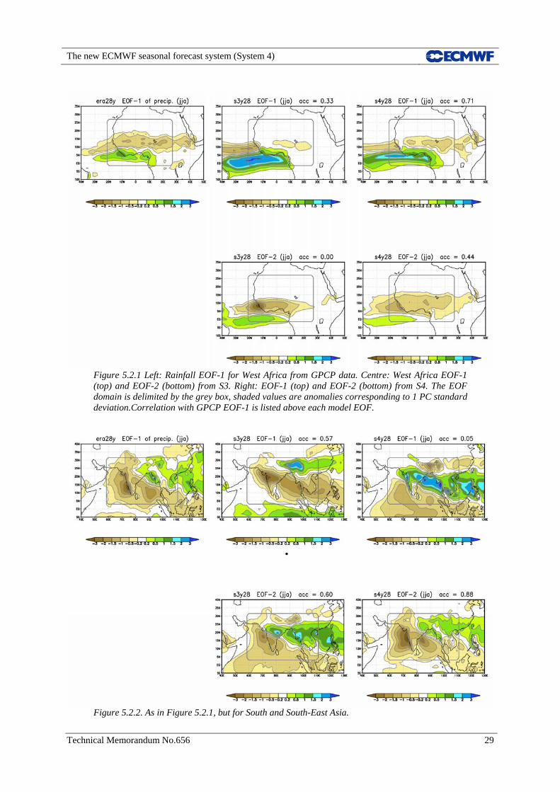
These results can be better understood by comparing the patterns of the GPCP EOF-1 with the first two model EOFs of both systems. Figure 5.2.1 shows the comparison for West Africa, and Figure 5.2.2 for South-SE Asia. For West Africa, the anti-correlation between rainfall along the Guinea Coast and the Sahel, represented by the GPCP EOF, is simulated by neither of the two leading EOFs of S3. In particular, EOF-1 of S3 had far too large amplitude over the ocean and coastal regions, with almost no signal over Sahel, while the dipolar structure in the S3 EOF-2 is shifted to the south and orthogonal to the GPCP EOF-1. As a result, in S3 no advantage is seen in using a 2-EOF subspace to predict the observed PC-1, and a 3-EOF subspace is needed to improve the PC correlation. Compared to S3, the first EOF of S4 is a far better match for the GPCP pattern, with negative anomalies over Sahel extending north of Lake Chad, although with reduced amplitude. For S4, the use of a 2-EOF model subspace is already adequate for the GPCP PC-1 prediction; the inclusion of the third EOF gives a much smaller benefit in S4 than in S3.
The new ECMWF seasonal forecast system (System 4)
Technical Memorandum No.656 29
Figure 5.2.1 Left: Rainfall EOF-1 for West Africa from GPCP data. Centre: West Africa EOF-1 (top) and EOF-2 (bottom) from S3. Right: EOF-1 (top) and EOF-2 (bottom) from S4. The EOF domain is delimited by the grey box, shaded values are anomalies corresponding to 1 PC standard deviation.Correlation with GPCP EOF-1 is listed above each model EOF.
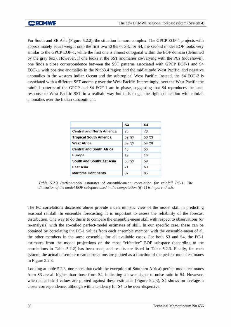
Figure 5.2.2. As in Figure 5.2.1, but for South and South-East Asia.
The new ECMWF seasonal forecast system (System 4)
30 Technical Memorandum No.656
For South and SE Asia (Figure 5.2.2), the situation is more complex. The GPCP EOF-1 projects with approximately equal weight onto the first two EOFs of S3; for S4, the second model EOF looks very similar to the GPCP EOF-1, while the first one is almost othogonal within the EOF domain (delimited by the gray box). However, if one looks at the SST anomalies co-varying with the PCs (not shown), one finds a close correspondence between the SST patterns associated with GPCP EOF-1 and S4 EOF-1, with positive anomalies in the Nino3.4 region and the midlatitude West Pacific, and negative anomalies in the western Indian Ocean and the subtropical West Pacific. Instead, the S4 EOF-2 is associated with a different SST anomaly over the West Pacific. Interestingly, over the West Pacific the rainfall patterns of the GPCP and S4 EOF-1 are in phase, suggesting that S4 reproduces the local response to West Pacific SST in a realistic way but fails to get the right connection with rainfall anomalies over the Indian subcontinent.
S3 S4
Central and North America 76 73
Tropical South America 69 (2) 50 (2)
West Africa 69 (3) 54 (3)
Central and South Africa 43 56
Europe 19 16
South and SouthEast Asia 53 (2) 59
East Asia 71 63
Maritime Continents 87 85
Table 5.2.3 Perfect-model estimates of ensemble-mean correlation for rainfall PC-1. The dimension of the model EOF subspace used in the computation (if>1) is in parenthesis.
The PC correlations discussed above provide a deterministic view of the model skill in predicting seasonal rainfall. In ensemble forecasting, it is important to assess the reliability of the forecast distribution. One way to do this is to compare the ensemble-mean skill with respect to observations (or re-analysis) with the so-called perfect-model estimates of skill. In our specific case, these can be obtained by correlating the PC-1 values from each ensemble member with the ensemble-mean of all the other members in the same ensemble, for all available cases. For both S3 and S4, the PC-1 estimates from the model projections on the most “effective” EOF subspace (according to the correlations in Table 5.2.2) has been used, and results are listed in Table 5.2.3. Finally, for each system, the actual ensemble-mean correlations are plotted as a function of the perfect-model estimates in Figure 5.2.3.
Looking at table 5.2.3, one notes that (with the exception of Southern Africa) perfect model estimates from S3 are all higher than those from S4, indicating a lower signal-to-noise ratio in S4. However, when actual skill values are plotted against these estimates (Figure 5.2.3), S4 shows on average a closer correspondence, although with a tendency for S4 to be over-dispersive.

The new ECMWF seasonal forecast system (System 4)
Technical Memorandum No.656 31
The tendency for S4 to under-estimate the signal-to-noise ratio for large-scale rainfall anomalies is in line with a general tendency of S4 to provide a better representation of the relationship between SST indices (such as Nino3.4, Indian Ocean Dipole, Southern Tropical Atlantic indices) and different atmospheric parameters on a global scale, but with a reduced intensity with respect to observation /re-analysis data. Regression maps of near-surface and tropospheric winds, precipitation and geop. height at 200 hPa have been computed from ERA-interim/GPCP, S3 and S4 (not shown for brevity), and normalised rms errors between model and observed regression patterns have been determined.
The average normalised error of such regressions decreases from 0.73 in S3 to 0.63 in S4, but the amplitude of the S4 regressions (in terms of eg. rms rainfall anomaly per 1 degree of SST variability) is usually between 60% and 80% of the amplitude of the observed regression. As far as the ENSO teleconnections are concerned, this error is partially compensated by the over-activity of El-Nino SST, but the forced signal from other tropical ocean regions remains partially underestimated.
In conclusion, although PC correlations obtained with the two systems are comparable in most regions, predictions of large-scale rainfall anomalies from S4 represent an improvement with respect to S3 mainly in terms of reliability and spatial correlation (with India being the notable exception as far the spatial teleconnections are concerned ). It should be noted that, with the exclusion of Europe (the only region considered where the EOF domain is entirely limited to the extratropics), predictions of the seasonal-mean GPCP PC-1 obtained by S4 forecasts exceed the 50% correlation level for all tropical and sub-tropical regions investigated here. Although the leading EOF accounts for just part of the total signal, our assessment indicates that seasonal predictions of rainfall anomalies over tropical continents contain potentially useful signals, which are often masked at grid-point level but can be extracted by a suitable statistical analysis.
Figure 5.2.3 Scatter diagrams of correlations between GPCP PC-1 and ensemble-mean forecasts (y-axis) against perfect model estimates of ensemble-mean correlation (x-axis), for S3 (left) and S4 (right).
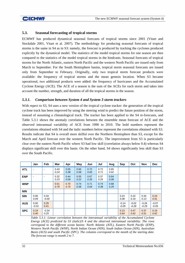
The new ECMWF seasonal forecast system (System 4)
32 Technical Memorandum No.656
5.3. Seasonal forecasting of tropical storms
ECMWF has produced dynamical seasonal forecasts of tropical storms since 2001 (Vitart and Stockdale 2001, Vitart et al. 2007). The methodology for producing seasonal forecasts of tropical storms is the same in S4 as in S3: namely, the forecast is produced by tracking the cyclones produced explicitly by the dynamical model. The statistics of the model tropical storms for one season are then compared to the statistics of the model tropical storms in the hindcasts. Seasonal forecasts of tropical storms for the North Atlantic, eastern North Pacific and the western North Pacific are issued only from March to September. For the South Hemisphere basins, tropical storm seasonal forecasts are issued only from September to February. Originally, only two tropical storm forecast products were available: the frequency of tropical storms and the mean genesis location. When S3 became operational, two additional products were added: the frequency of hurricanes and the Accumulated Cyclone Energy (ACE). The ACE of a season is the sum of the ACEs for each storm and takes into account the number, strength, and duration of all the tropical storms in the season.
5.3.1. Comparison between System 4 and System 3 storm trackers
With repect to S3, S4 uses a new version of the tropical cyclone tracker: the generation of the tropical cyclone track has been improved by using the steering wind to predict the future position of the storm, instead of assuming a climatological track. The tracker has been applied to the S4 re-forecasts, and Table 5.3.1 shows the anomaly correlations between the ensemble mean forecast of ACE and the observed interannual variability of ACE from 1990 to 2010. The bold numbers represent the correlations obtained with S4 and the italic numbers below represent the correlations obtained with S3. Results indicate that S4 is overall more skilful over the Northern Hemisphere than S3, except for the March and April forecast over the western North Pacific. The improvement from S3 is particularly clear over the eastern North Pacific where S3 had low skill (correlation always below 0.4) whereas S4 displays significant skill over this basin. On the other hand, S4 shows significantly less skill than S3 over the South Pacific.
Jan Feb Mar Apr May Jun Jul Aug Sep Oct Nov Dec
ATL - - 0.43 0.24
0.55 0.38
0.65 0.58
0.72 0.65
0.72 0.71
0.65 0.62
ENP - - 0.32 0.23
0.44 0.09
0.55 0.22
0.67 0.35
0.37 0.26
0.64 0.08
WNP 0.51 0.76
0.70 0.75
0.74 0.58
0.71 0.64
0.74 0.38
0.68 0.29
NIN
SIN 0.06 0.09
0.34 -0.00
0.24 0.08
0.22 0.16
0.34 0.13
0.24 0.51
AUS 0.00 -0.01
0.25 0.41
-0.14 -0.05
-0.02 -0.28
-0.26 -0.29
-0.07 -0.05
SPC 0.19 0.40
-0.34 0.25
0.13 0.64
0.47 0.62
0.37 0.51
0.19 0.62
Table 5.3.1: Linear correlation between the interannual variability of the Accumulated Cyclone Energy (ACE) predicted by S3 (italic)/S 4 and the observed interannual variability. The rows correspond to the different ocean basins: North Atlantic (ATL), Eastern North Pacific (ENP), Western North Pacific (WNP), North Indian Ocean (NIN), South Indian Ocean (SIN), Australian Basin (AUS) and south Pacific (SPC). The columns correspond to the month of the starting date. The forecast range is month 2 to 7.

The new ECMWF seasonal forecast system (System 4)
Technical Memorandum No.656 33
Figure 5.3.1: Interannual variability of the number of typhoons observed (red curves) and predicted by S4 (blue curve in top panel) and S3(blue curve in bottom panel) for the period July to December 1990-2010. The forecasts start on 1st June. The green vertical lines represent 2 standard deviations from the model ensemble distribution.

The new ECMWF seasonal forecast system (System 4)
34 Technical Memorandum No.656
S4 displays similar improvements for the frequency of tropical storms or hurricanes over the northern hemisphere. A large part of this improvement over the northern Hemisphere is due to a better simulation of the decadal trends. For instance, figure 5.3.1 shows that the observed negative trend in the number of hurricanes over the western North Pacific is present in the S4 forecasts, but not in the S3 forecasts. This improvement in the simulation of decadal trends of tropical storms comes from a good simulation of inter-decadal variability in tropical wind shear.
5.3.2. Tropical storm density anomalies
The tropical storm genesis location and tropical storm tracks can display a strong interannual variability. For instance, ENSO has a very strong impact on the location of cyclogenesis over the western and eastern North Pacific. In S3, forecasts of the mean genesis location for each basin are issued, since it was found that S3 displays some skill in predicting shifts in the genesis location of tropical storms due to ENSO (Vitart and Stockdale 2001). In S4, this product is going to be replaced by a tropical storm density anomaly map which should be more informative than the mean genesis location: for each grid point, the number of tropical storm tracks passing within 300 km during a season is calculated, and the anomalies relative to the model climate are displayed. Figure 5.3.2 shows the linear correlation for each grid point between the observed and predicted density anomaly of tropical storms for the forecasts starting on 1st May 1991-2010. This figure shows that S4 has significant skill in predicting the density anomaly of tropical storms. In particular, the model simulates a realistic east-west shift in the location of tropical storms over the western North Pacific, and a south-west/north-east shift of tropical storm activity over the eastern North Pacific during El-Nino and La-Nina years, in agreement with observations (not shown). The density of tropical storms in the model is also sensitive to local SST anomalies as observed.
Figure5.3.2: Linear correlation (%) between the observed and predicted interannual variability of tropical storm density for each grid point for the period July to December and for the forecasts starting on 1st May 1990-2010.
5.4. Experimentation with momentum flux-correction
The ECMWF atmospheric model (IFS) undergoes continual development, and in the years since S3 was introduced many changes to the model have been made. These changes have led to many improvements in the medium and monthly range forecasts, and in many aspects of the model climate on seasonal timescales. However, there is no guarantee that all changes will be beneficial for the seasonal forecasting system.

The new ECMWF seasonal forecast system (System 4)
Technical Memorandum No.656 35
Figure 5.4.1 shows the systematic error in the near-surface zonal wind for S3 and S4 in JJA at 2-to-4 month forecast range. Focusing on the western part of the tropical Pacific, we see that the bias has increased in S4, although mean errors in the eastern Pacific and equatorial Indian Ocean have been reduced. This change in bias is also present in atmosphere-only simulations, and appeared after the introduction of model cycle 32r3, which included a revised convection scheme as well as a number of other modifications to the model physics. The improvement in extratropical biases and medium range forecast skill due to 32r3 is well documented in Bechtold et al. (2008) and Jung et al. (2010). However, the increased easterly winds in the tropical Pacific give rise to a positive feedback in the coupled model. The stronger winds strengthen the equatorial cold tongue (See Sect. 3.1) and enhance the Walker circulation, which leads to even stronger easterly winds.
Figure 5.4.1. Bias of 10m U-wind in the Jun-to-Aug season from S3 (top) and S4 re-forecasts.
The possibility of using momentum flux correction to push the mean state to a more realistic regime was investigated during the development of S3 (Anderson et al, 2007). Experience then showed a particular sensitivity of Nino 4 SST forecast performance to the mean state, and that this could be controlled by specifying an additive correction to the wind stress. Given the nature of the biases in cycles leading up to S4, several experiments were undertaken to assess the benefit of correcting atmospheric model errors in wind stress. In a typical experiment, the flux correction to be used is calculated from the difference between stresses from a given IFS run with observed SST, and stresses taken from ERA Interim. For cycle 36r1, which had a large bias problem, the effect of applying flux correction to the forecast system was very positive, and led to a big improvement in ENSO scores. However, cycle 36r4 had a (partially) reduced bias, and preliminary experiments suggested the gain from flux correction was much reduced. In order to maintain a closer synergy among all ECMWF

The new ECMWF seasonal forecast system (System 4)
36 Technical Memorandum No.656
ensemble systems, it was decided to proceed with building the S4 configuration assuming that flux correction would not be used. Once the S4 configuration was essentially complete, some final tests were run to assess the impact of flux correction. The tests were run at T159 and extended to the annual range, since this was considered as a possible configuration for the annual range forecasts. For brevity, only results from this final set of experiments are presented here.
To estimate the error in the uncoupled IFS model, a 5 member ensemble was run for the 22 year period 1989-2010, and the surface momentum fluxes compared to ERA interim. A monthly mean correction dataset was derived, with a 1-2-1 smoothing across adjacent months to minimize noise at higher latitudes. Two sets of otherwise identical forecast experiments were then run, one a control and one with a correction to the surface fluxes as passed from the atmosphere to the ocean model.
Figure 5.4.2 shows the mean difference in JJA 2-metre temperature between the control experiment (using the S4 configuration with no flux correction) and the experiment with flux correction (both started on 1 May); negative values means that the control experiment is colder. Regarding the tropical Pacific it is evident that the cold bias could be effectively reduced by using momentum flux correction, due to less upwelling of cold water. (Note that, consistently with observed teleconnections, the cold bias in the eastern tropical Pacific leads to a cooling in the Sahel associated with wetter conditions).
Figure 5.4.2. Mean difference in 2-metre temperature in JJA between experiments with and without flux correction started on 1 May.
Figure 5.4.3 shows examples of seasonal forecasts of the SST in the NINO3.4 area from S3 (green), S4 (blue) and S4 + flux correction (red), starts in May 1995, 1996 and 1997. Comparing the simulations with and without flux correction, we see the fast development of the cold bias for the non flux-corrected forecasts. However, it seems like flux corrected forecasts occasionally develop similar biases (one ensemble member from 1995 and one from 1996 show a notable drift). In general, the flux-corrected forecast seems to stay much closer to the observed values and the results for S3 than the non-flux corrected ones.

The new ECMWF seasonal forecast system (System 4)
Technical Memorandum No.656 37
Figure 5.4.3. Forecasts initialised in May 1995, 1996 and 1997 for the SST in NINO3.4 (daily values) for S3 (green), S4 without correction (blue) and S4 with flux correction (red). Observed values in black.
Panel (a) in Figure 5.4.4 shows the mean model drift in SST from the NINO3.4 area for forecasts initialised in February, May, August and November. The fastest drift occurs during the boreal summer months for the non flux-corrected experiment. For the flux-corrected experiment most of the drift is removed, but there seem to be some errors in capturing the seasonal cycle of the SST. As a measure of model activity, panel (b) of the same figure shows the rms amplitude ratio of the anomalies (modelled divided by observed amplitude) as a function of lead time. For the non flux-corrected experiment the activity is too high compared to the observed ones during the first 6 months (consistent with results in Sect. 3.2), while the latter part of the integrations shows a moderate under-activity. The enhanced activity during the first months may be partly an effect of the onset of the model drift, which can be shifted in time between forecasts.
(a) (b)
Figure 5.4.4. Left: Drift in Nino3.4 SST for S4 experiment with (red) and without (blue) flux correction. Right: NINO3.4 SST anomaly amplitude ratio with respect to observed anomalies for experiment with (red) and without (blue) flux correction.

The new ECMWF seasonal forecast system (System 4)
38 Technical Memorandum No.656
In Figure 5.4.5a the anomaly correlation scores for the Nino3.4 are plotted. One should here bear in mind that these scores are based on a limited set of experiments, both in terms of initial dates and ensemble members. Before the scores were calculated, a lead-time dependent bias correction has been applied. According to these SST scores, using flux-correction slightly improves the forecast quality, although the impact is quite modest and can hardly justify the introduction of flux correction in the S4 operational configuration. The difference in skill is largest in the western part of the tropical Pacific (NINO4, not shown). For Nino3.4, the difference in skill seems largest for February start dates and more or less neutral for August start dates.
(a) (b)
Figure 5.4.5. Anomaly correlation coefficients for experiments with (red) and without (blue) flux correction in the Nino3.4 region. Left: ACC for SST anomaly. Right: ACC for rainfall anomaly.
While for the SST forecast a bias correction can be applied as post-processing, the cold bias has a direct effect on atmospheric processes in the coupled system, such as precipitation. In the presence of a strong cold bias, convection over the tropical ocean is inhibited. Even if a warm anomaly is detected in the SST forecast, the effect on the atmospheric convection is much less than in a unbiased simulations. This has a negative effect on the correlation scores for precipitation in the NINO3.4 region (Figure 5.4.5b), where we see a clear advantage for the flux-correction experiment.
In summary, experimentation with flux correction shows a potential for further improvements in ENSO forecasting (partially in terms of SST forecast skill but more so in terms of associated heating anomalies and teleconnections) if the systematic error for the tropical Pacific surface winds could be alleviated in future cycles of the atmospheric model.
6. Conclusions
In the last two decades, seasonal forecasts provided by a number of institutions have evolved from experimental to operational stage. Prediction systems based on coupled ocean-atmosphere models have gradually improved their superiority over statistical systems as far as predictions of ENSO events are concerned. International, coordinated efforts have led to extensive intercomparison of large re-forecast set and production of operational multi-model products (Palmer et al. 2004; Jin et al. 2008; Wang et al. 2009; Weisheimer et al. 2009)
ECMWF has been at the forefront of these research and operational efforts since their earlier stages, not only with our own operational systems, but also in the coordination of e.g. the PROVOST and DEMETER projects, and the implementation of the seasonal EUROSIP multi-model system in

The new ECMWF seasonal forecast system (System 4)
Technical Memorandum No.656 39
collaboration with Meteo France and the UK Met Office. The current ECMWF S3 has gained the reputation of a highly skilful ENSO prediction system (with the highest skill among the ENSO forecast systems compared by Barnston et al. 2011). However, S3 was not without problems (for example, predictions of tropical Atlantic SST were often no better than persistence, monsoon systems in West Africa and South Asia suffered from large errors, sea-ice variability was neglected), and its ocean model/analysis component was no longer state-of-the-art.
System 4 has been developed with the goals of improving those aspects where S3 was deficient, and posing the foundations for future progress in ocean and sea-ice modelling. With respect to S3 (and to seasonal systems from most other operational centres), S4 has the advantage of providing a 30-year re-forecast set initialised from, and verified against, a single state-of-the-art re-analysis for both the atmosphere (ERA-interim) and the ocean (the NEMOVAR based ORA-S4). Progress in physical parametrizations has led to substantial bias reductions in extratropical regions, and more realistic tropical intra-seasonal variability. Increased horizontal and vertical resolution has been introduced with the goal of providing a better representation of regional and/or extreme anomalies.
This report has summarised the methodologies and discussed the most relevant results obtained so far from the re-forecast set. Some of the notable results include:
very high levels of skill for ENSO forecasts, with further progress on the anomaly correlation of ENSO indices in most areas and seasons;
a clear improvement in the simulation and prediction of ocean/atmosphere variability in the tropical Atlantic and adjacent regions (eg West African monsoon);
more reliable predictions for extratropical regions, which improve on S3 in terms of both deterministic and probabilistic scores;
better simulation of inter-annual and decadal variability of tropical storm properties.
As with any new operational systems, not every change is for the better. System 4 suffers from a stronger cold bias in tropical Pacific SST than S3, and this is reflected in a lack of improvement in West Pacific scores and too large variability in ENSO SST indices. The incorrect relationship between West Pacific and Indian rainfall during the monsoon season may also be related to this problem, although a suitable EOF mapping is able to extract significant correlation between observed and modelled patterns of rainfall variability over South Asia. Experiments with momentum flux correction indicate that biases in Pacific trade winds simulated by the atmospheric model are the main source of the coupled model drift, and show the potential for further progress.
With regard to this problem, one should point out that experimentation done during the development of S4 has been instrumental in highlighting long-term model biases which are not apparent at shorter forecast ranges. System 4 has incorporated new developments in land-surface modelling and initialization procedures, providing valuable feedbacks to the development work carried out in the Physical Aspects section. Useful guidance has been obtained on the most appropriate setting of stochastic terms for the simulation of model uncertainties. Last but not least, the introduction of a new modelling and analysis environment for the ocean will benefit EPS predictions across a wide range of

The new ECMWF seasonal forecast system (System 4)
40 Technical Memorandum No.656
time scales. These interactions testify the continued feedback between the extended and medium-range forecasting activities of ECMWF.
A few words should be also said on how S4 is going to allow ECMWF to fulfill its role as a WMO Global Producing Centre for Long Range Forecasting. As highlighted by the current dramatic situation in part of East Africa, interannual rainfall variability continues to be a major factor affecting health and food production in many tropical and sub-tropical countries. System 4 represents a step forward in representing large-scale rainfall anomalies which are closer to their observed counterparts in terms of amplitude and spatial pattern. This is particularly true for Africa and South America, with West Africa showing the clearest improvements in terms of both spatial and temporal correlations. As far as the Asian monsoon systems are concerned, progress is more patchy: System 4 is responsive to SST signals which affect the South and SE Asian monsoon, but the relationship between rainfall anomalies in different regions is not yet properly represented, and the predicted signal needs a proper statistical mapping to be exploited.
Even before S4 is implemented, work has already been started on areas where the new system leaves scope for improvement. Horizontal and vertical resolution in the ocean model represents the main development area in the next few years, and experimentation with a ¼ degree, 75-level version of NEMO is going to start before the end of the year. Progress is expected especially in the representation of the mean state and variability of the western boundary currents, with possible beneficial impacts on extratropical predictability. The dynamical sea-ice model LIM-2 (Fichefet and Morales Maqueda, 1997) has already been incorporated into the coupled model in research mode, and assessment of the impact of sea-ice variability on potential predictability in the North Atlantic and Europe is under way. Further progress in land surface modelling and initialization is expected in the next two years, with better treatment of lakes and snow variability. An off-line version of the new land-surface analysis scheme will be used to explore sensitivity to land-surface perturbations, an area currently neglected in our ensemble generation strategy. Further contributions to predictability are also expected from a better treatment of stratospheric processes as well as ozone and aerosol variability. Work in these areas is expected to improve all ECMWF probabilistic forecast systems.
In conclusion, the new System 4 is a further step forward along a line of world-leading seasonal forecast systems developed at ECMWF. These are providing ECMWF Member States with high quality information for a number of application areas, and ECMWF scientists with additional modelling tools and valuable diagnostics, at a modest cost in terms of human and computational resources. Equally important is the contribution that the System 4 operational forecasts, re-forecast set and ocean re-analysis give to international efforts on seasonal prediction at both research and operational level, maintaining a position of leadership for European science which is widely recognized and appreciated by national and international institutions.

The new ECMWF seasonal forecast system (System 4)
Technical Memorandum No.656 41
Acknowledgements
The authors are grateful to many colleagues in the ECMWF Research and Operations Departments for their contribution to the development of System-4. The collaboration of of Martin Leutbecher on the optimization of the stochastic schemes and the efforts of staff in the Physical Aspects Section are much appreciated. In particular, recent changes to the moist physics, the radiation scheme and the land surface model have led to a more realistic model variability, better predictability and reduced systematic errors.
References
Anderson, D., T. Stockdale, M. Balmaseda, L. Ferranti, F. Vitart, F. Molteni, F. Doblas-Reyes, K. Mogensen and A. Vidard, 2007: Development of the ECMWF seasonal forecast System 3. ECMWF Technical Memorandum 503.
Balmaseda M., A. Vidard, D.L.T. Anderson 2008. The ECMWF ocean analysis system: ORA-S3. Mon. Wea. Rev., 136, 3018-3034.
Balsamo, G., R. Salgado, E. Dutra, S. Boussetta, T. Stockdale and M. Potes, 2011: On the contribution of lakes in predicting near-surface temperature in a global weather forecasting model. ECMWF Tech. Memorandum 648.
Barnston, A.G., M. K. Tippett, M.L. L’Heureux, S. Li, and D.G. DeWitt, 2011: Skill of Real-time Seasonal ENSO Model Predictions during 2002-2011—Is Our Capability Increasing? Bull. American Met. Society, submitted.
Bechtold, P., M. Köhler, T. Jung, F. Doblas-Reyes, M. Leutbecher, M.J. Rodwell. F. Vitart and G. Balsamo, 2008: Advances in simulating atmospheric variability with the ECMWF model: From synoptic to decadal time-scales. Q.J.R.Meteorol.Soc., 134, 1337-1351.
Brankovic, C., T.N. Palmer, F. Molteni, S. Tibaldi and U. Cubasch, 1990: Extended-range predictions with ECMWF models: Time-lagged ensemble forecasting. Q.J.R.Meteorol.Soc., 116, 867-912.
Cagnazzo, C. and E. Manzini, 2009: Impact of the stratosphere on the winter tropospheric teleconnections between ENSO and the North Atlantic and European region. J. Clim. 1223-1238.
Feudale, L. and A.M. Tompkins, 2011: A simple bias correction technique for modeled monsoon precipitation applied to West Africa. Geophys. Res. Letters, 38 (3), L03803.
Fichefet, T., and M.A. Morales Maqueda, 1997: Sensitivity of a global sea ice model to the treatment of ice thermodynamics and dynamics. J. Geophys. Res., 102, 12609-12646.
Jin, E. K, J. L. Kinter III, B. Wang and Co Authors, 2008: Current status of ENSO prediction skill in coupled ocean-atmosphere model. Clim. Dyn., 31, 647-664, DOI:10.1007/s00382-008-0418-2.

The new ECMWF seasonal forecast system (System 4)
42 Technical Memorandum No.656
Jung, T., G. Balsamo, P. Bechtold, A.C.M. Beljaars, M. Köhler, M.J. Miller, J-J. Morcrette, A. Orr, M.J. Rodwell and A.M. Tompkins, 2010: The ECMWF model climate: recent progress through improved physical parametrizations. Q.J.R.Meteorol.Soc., 136, 1145–1160, doi:10.1002/qj.634.
Madec G. 2008. NEMO reference manual, ocean dynamics component: NEMO-OPA. Note du Pole de Modelisation 27, Institut Pierre-Simon Laplace (IPSL), France.
Marshall, A.G. and A.A. Scaife, 2009: Impact of the QBO on surface winter climate. J. Geophys. Res. 114, D18110. doi:10.1029/2009JD011737.
Molteni, F., U. Cubasch and S. Tibaldi, 1987: 30 and 60-day forecast experiments with the ECMWF spectral models. Proceedings of the first ECMWF Workshop on Predictability in the medium and extended range (ECMWF, Reading, U.K., 17-19 Mar. 1986), 51-108.
Molteni, F. , F. Vitart, T. Stockdale, L. Ferranti and M. Balmaseda, 2008: Predictions of tropical rainfall with the ECMWF seasonal and monthly forecast systems. Proceedings of the ECMWF Workshop on Ensemble Prediction (7-9 November 2007), 117-132.
Palmer, T.N. and D.L.T. Anderson, 1994: The prospects for seasonal forecasting - A review paper. Q.J.R.Meteorol.Soc., 120, 755-793.
Palmer, T.N., A. Alessandri, U. Andersen, P. Cantelaube, M. Davey, P. Délécluse, M. Déqué, E. Díez, F.J. Doblas-Reyes, H. Feddersen, R. Graham, S. Gualdi, J.-F. Guérémy, R. Hagedorn, M. Hoshen, N. Keenlyside, M. Latif, A. Lazar, E. Maisonnave, V. Marletto, A. P. Morse, B. Orfila, P. Rogel, J.-M. Terres, M. C. Thomson, 2004. Development of a European multi-model ensemble system for seasonal to inter-annual prediction (DEMETER). Bull. American Met. Society, 85, 853-872
Palmer, T.N., R. Buizza, F. Doblas-Reyes, T. Jung, M. Leutbecher, G.J. Shutts, M. Steinheimer and A Weisheimer, 2009: Stochastic parametrization and model uncertainty. ECMWF Technical Memorandum 598.
Shindell, D.T., G.A. Schmidt, M.E. Mann and G. Faluvegi, 2004: Dynamic winter climate response to large tropical volcanic eruptions since 1600. J. Geophys. Res. 109, D05104. doi: 10.1029/2003JD004151.
Stockdale, T.N., D.L.T. Anderson, J.O. Alves and M.A. Balmaseda, 1998: Global seasonal rainfall forecasts with a coupled ocean atmosphere model. Nature, 392, 370-373.
Stockdale, T.N., D. L. T. Anderson, M. A. Balmaseda, F. Doblas-Reyes, L. Ferranti, K. Mogensen, T.N. Palmer, F. Molteni and F. Vitart, 2011: ECMWF seasonal forecast system 3 and its prediction of sea surface temperature. Clim. Dyn. doi 10.1007/s00382-010-0947-3
Vitart, F., and T.N. Stockdale, 2001: Seasonal forecasting of tropical storm using coupled GCM integrations. Mon. Wea. Rev, 129(10), 2521-2527.

The new ECMWF seasonal forecast system (System 4)
Technical Memorandum No.656 43
Vitart, F., M. Huddleston, M. Deque, D. Peake, T. Palmer, T. Stockdale, M. Davey, S. Ineson and A. Weisheimer, 2007: Dynamically-based seasonal forecast of Atlantic tropical storm activity issued in June by EUROSIP. Geophys. Res. Lett., 34, L16815, doi:10.1029/2007GL030740.
Wang, B., J-Y. Lee, J. Shukla, I.-S. Kang, C.-K. Park and co-authors, 2009: Advance and prospectus of seasonal prediction: Assessment of APCC/CliPAS 14-model ensemble retrospective seasonal prediction (1980-2004). Clim. Dyn. 33, 93-117, DOI:10.1007/s00382-008-0460-0.
Weisheimer, A., F.J. Doblas-Reyes, T.N. Palmer, A. Alessandri, A. Arribas, M. Deque, N. Keenlyside, M. MacVean, A. Navarra and P. Rogel, 2009: ENSEMBLES - a new multi-model ensemble for seasonal-to-annual predictions: Skill and progress beyond DEMETER in forecasting tropical Pacific SSTs. Geophys. Res. Lett., 36, L21711, doi:10.1029/2009GL040896.
Wolff, J., E. Maier-Reimer and S. Legutke, 1997. The Hamburg Ocean Primitive Equation Model. Deutsches Klimarechenzentrum, Hamburg, Technical Report No. 13.
WCRP, 2008: WCRP Position Paper on Seasonal Prediction - Report from the First WCRP Seasonal Prediction Workshop (Barcelona, Spain, 4-7 June 2007). Lead authors: B. Kirtman and A. Pirani. WCRP Informal Report No. 3/2008 - ICPO Publication No. 127.

The new ECMWF seasonal forecast system (System 4)
44 Technical Memorandum No.656
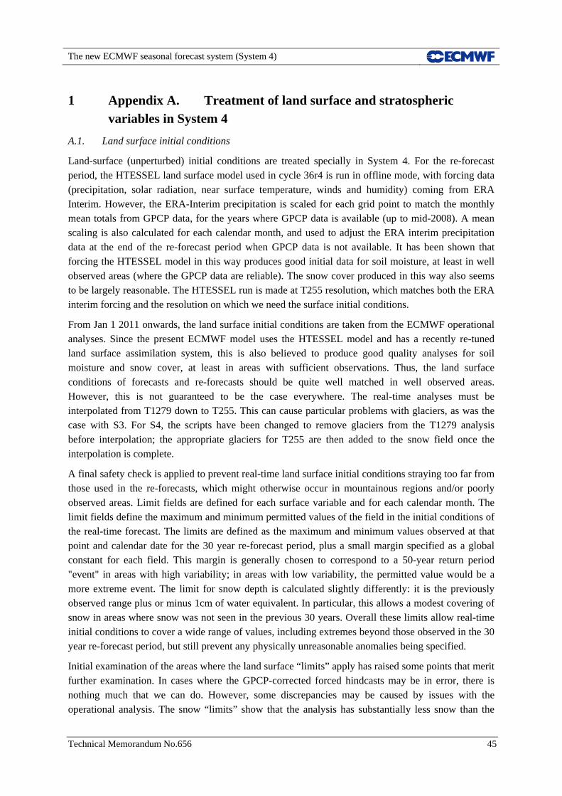
The new ECMWF seasonal forecast system (System 4)
Technical Memorandum No.656 45
1 Appendix A. Treatment of land surface and stratospheric variables in System 4
A.1. Land surface initial conditions
Land-surface (unperturbed) initial conditions are treated specially in System 4. For the re-forecast period, the HTESSEL land surface model used in cycle 36r4 is run in offline mode, with forcing data (precipitation, solar radiation, near surface temperature, winds and humidity) coming from ERA Interim. However, the ERA-Interim precipitation is scaled for each grid point to match the monthly mean totals from GPCP data, for the years where GPCP data is available (up to mid-2008). A mean scaling is also calculated for each calendar month, and used to adjust the ERA interim precipitation data at the end of the re-forecast period when GPCP data is not available. It has been shown that forcing the HTESSEL model in this way produces good initial data for soil moisture, at least in well observed areas (where the GPCP data are reliable). The snow cover produced in this way also seems to be largely reasonable. The HTESSEL run is made at T255 resolution, which matches both the ERA interim forcing and the resolution on which we need the surface initial conditions.
From Jan 1 2011 onwards, the land surface initial conditions are taken from the ECMWF operational analyses. Since the present ECMWF model uses the HTESSEL model and has a recently re-tuned land surface assimilation system, this is also believed to produce good quality analyses for soil moisture and snow cover, at least in areas with sufficient observations. Thus, the land surface conditions of forecasts and re-forecasts should be quite well matched in well observed areas. However, this is not guaranteed to be the case everywhere. The real-time analyses must be interpolated from T1279 down to T255. This can cause particular problems with glaciers, as was the case with S3. For S4, the scripts have been changed to remove glaciers from the T1279 analysis before interpolation; the appropriate glaciers for T255 are then added to the snow field once the interpolation is complete.
A final safety check is applied to prevent real-time land surface initial conditions straying too far from those used in the re-forecasts, which might otherwise occur in mountainous regions and/or poorly observed areas. Limit fields are defined for each surface variable and for each calendar month. The limit fields define the maximum and minimum permitted values of the field in the initial conditions of the real-time forecast. The limits are defined as the maximum and minimum values observed at that point and calendar date for the 30 year re-forecast period, plus a small margin specified as a global constant for each field. This margin is generally chosen to correspond to a 50-year return period "event" in areas with high variability; in areas with low variability, the permitted value would be a more extreme event. The limit for snow depth is calculated slightly differently: it is the previously observed range plus or minus 1cm of water equivalent. In particular, this allows a modest covering of snow in areas where snow was not seen in the previous 30 years. Overall these limits allow real-time initial conditions to cover a wide range of values, including extremes beyond those observed in the 30 year re-forecast period, but still prevent any physically unreasonable anomalies being specified.
Initial examination of the areas where the land surface “limits” apply has raised some points that merit further examination. In cases where the GPCP-corrected forced hindcasts may be in error, there is nothing much that we can do. However, some discrepancies may be caused by issues with the operational analysis. The snow “limits” show that the analysis has substantially less snow than the
The new ECMWF seasonal forecast system (System 4)
46 Technical Memorandum No.656
offline run in a narrow band down the coastal edge of the mountains in Norway and Canada. Others have also noticed the possible lack of snow in our analysis for the Norwegian mountains. Given the inherent difficulties in producing snow analyses in mountainous terrain, this may be worth attention. A further fascinating point is soil moisture values around Lake Victoria – the soil is very dry in the analysis. It is hard to think of a physical reason for the soil near the lake being so dry, and it may be that a mismatch between modelled and observed humidity near the lake is causing unrealistic moisture increments in the analysis. In either of these cases, if a problem is found and corrected in the analysis, it will lead to better consistency between the re-forecasts and future forecasts.
A.2 Stratosphere and volcanic aerosols
In System 4, stratospheric volcanic aerosols are taken into account within the forecast system. Only very approximate values are specified - three numbers giving NH, tropical and SH amounts respectively, together with assumed vertical profiles. Values are specified using data from the month before the forecast starts, and then damped persistence applies during the forecast. Thus major eruptions are not captured in advance, but the after effects can be accounted for to some extent in the forecasts. It would be preferable to have a better characterization of volcanic aerosol distribution and properties, and eventually a real-time analysis systems should be able to provide such information. For the time being, however, we specify data in the re-forecasts with a similar level of accuracy to what we think might be achieved in real-time. As yet we do not have an operational method in place to provide current aerosol values. After the May 2011 eruption of Grimsvotn in Iceland this is becoming an issue that needs to be addressed. As an interim measure, we are using MACC-related SO2 analyses to give integrated amounts of SO2 at times of relevant volcanic eruptions, combined with USGS/Smithsonian Weekly Volcanic Activity Report to estimate how much of the SO2 might plausibly have been injected into the stratosphere. This can then be compared with estimates of SO2 injection from previous eruptions, to allow a rough estimate of the amount of sulphate aerosol that might form in the weeks after the eruption. In the case of Grimsvotn, this method suggests that the amount of aerosol can be no more than moderate, and is definitely much smaller than the eruptions of e.g. Pinatubo or El Chichon. This approach can be checked against visual inspection of LIDAR-based profiles from the CALIPSO satellite. Distinguishing sulphate aerosol from cloud traces in the lower stratosphere is not immediately straightforward, but any substantial amount of aerosol above 18km is expected to become apparent in this data. It is hoped that less ad-hoc monitoring methods can be developed.
Solar variation is applied to the total solar irradiance, without any spectral discrimination. For the UV bands in the ECMWF radiation scheme, the specified UV variability is thereby up to 30 times smaller than it should be. The processes by which the 11 year solar cycle drives variations in the stratosphere are thus largely missing from the model. The prediction of the evolution of the QBO phase in the model is also deficient, despite the re-tuning of some of the stratospheric physics. Although there are likely to be errors in both the resolved and parameterized gravity wave sources in the tropical troposphere, the vertical resolution of the model is in any case inadequate to model the QBO accurately in a quantitative sense. Future work to improve the accuracy of interannual variability in the stratosphere should benefit from both a better specification of solar variations and the availability of higher vertical resolution (c. 137 levels).

The new ECMWF seasonal forecast system (System 4)
Technical Memorandum No.656 47
2 Appendix B – Characteristics of the extended-range forecast systems operational and under development at ECMWF, UKMO, Météo France, NCEP, MSC, JMA and BOM.
Current systems spanning the sub-seasonal and seasonal time range Known planned changes for 2011-12
ECMWF
d0-d15/32: ECMWF EPS/monthly (twice a day to 15d and once a week to 32d) TL639(d0-10)v319(d10-15)L62, TOA 5hPa, 50+1 members. 15d fc range, extended to 32d every Thu, with persisted SST up to d10 and coupled HOPE (1:1/3 degree resolution, L40) ocean model from day 10. Initial uncertainties simulated using TL399L91 EDA- and T42L62 SV-based perturbations Model uncertainties simulated using SPPT and SKEB stochastic schemes. Re-forecast suite with 5 members run once a week for 18 years. m1-7/13: ECMWF S3 (once a month to m7 and every quarter to m13) 41 members with TL159L40 resolution, with coupled HOPE (1:1/3 degree resolution, L29) ocean model. Frozen model cycle (cy31r1). Re-forecast suite with 11 members, 25 years Part of EUROSIP.
d0-d15/32: Twice-weekly 32d extension (Mon and Thu at 00UTC). Use of NEMO (ORCA1 with tripolar grid: 1:1/3 degree resolution, Z42) instead of HOPE ocean model. m1-7/13: ECMWF S4 51 members with TL255L91 resolution, with NEMO ocean model (ORCA1: 1-1/3 degree resolution, Z42). Re-forecasts: 15 members, 30 years. Frozen model cycle (36r4).
UK Met Office
d0-15: MOGREPS15 (twice a day) N216L70 (~50km), TOA ~80km, 24 members. Initial perturbations simulated using ETKF. Model uncertainties simulated using perturbed physics and stochastic backscatter (SKEB) schemes. Uncoupled. d0-60: UKMO monthly system (once a week) The monthly system is under testing: it is part of the seasonal system. N96 (~120km resolution) L85 with NEMO ocean model (ORCA1, i.e. 1:1/3 degree, L75 resolution). 28 members run in lagged mode (4 members per day). m1-7: UKMO seasonal system (once a month) N96 (~120km resolution) L85 with coupled NEMO ocean model (ORCA1L75 resolution). 42 members run in lagged mode (14 members per week). Reforecast suite with 12 members, 14 years (1996-2009). Part of EUROSIP.
d0-15: 4 runs per day with 12 members, 40 km horizontal resolution. d0-60: increase resolution to N216 in late 2011.
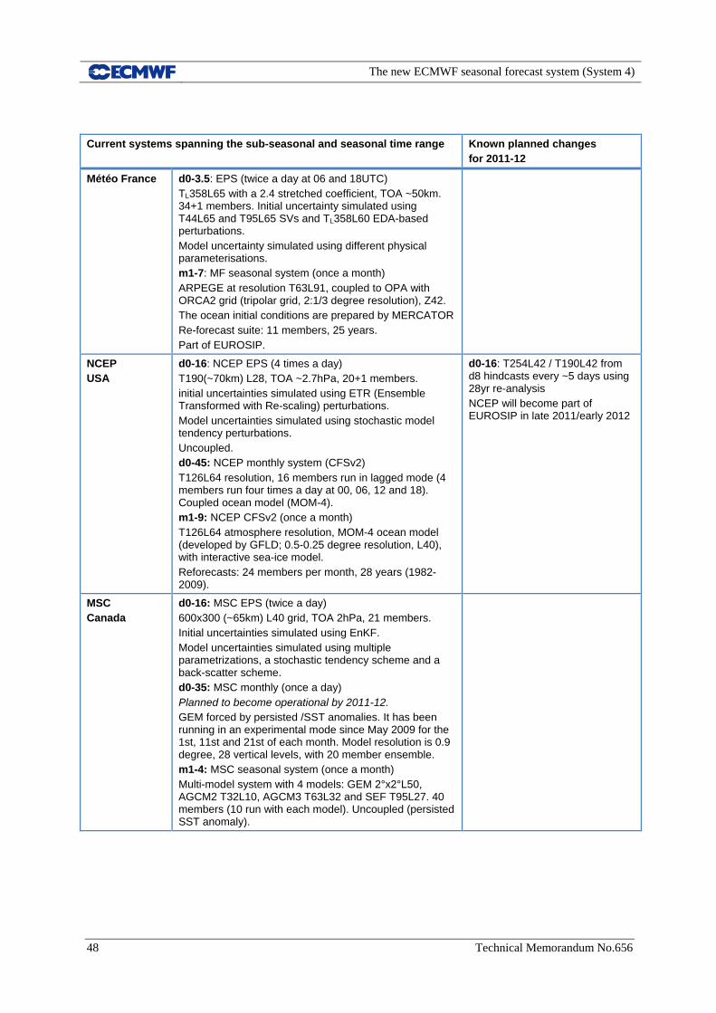
The new ECMWF seasonal forecast system (System 4)
48 Technical Memorandum No.656
Current systems spanning the sub-seasonal and seasonal time range Known planned changes for 2011-12
Météo France
d0-3.5: EPS (twice a day at 06 and 18UTC) TL358L65 with a 2.4 stretched coefficient, TOA ~50km. 34+1 members. Initial uncertainty simulated using T44L65 and T95L65 SVs and TL358L60 EDA-based perturbations. Model uncertainty simulated using different physical parameterisations. m1-7: MF seasonal system (once a month) ARPEGE at resolution T63L91, coupled to OPA with ORCA2 grid (tripolar grid, 2:1/3 degree resolution), Z42. The ocean initial conditions are prepared by MERCATOR Re-forecast suite: 11 members, 25 years. Part of EUROSIP.
NCEP USA
d0-16: NCEP EPS (4 times a day) T190(~70km) L28, TOA ~2.7hPa, 20+1 members. initial uncertainties simulated using ETR (Ensemble Transformed with Re-scaling) perturbations. Model uncertainties simulated using stochastic model tendency perturbations. Uncoupled. d0-45: NCEP monthly system (CFSv2) T126L64 resolution, 16 members run in lagged mode (4 members run four times a day at 00, 06, 12 and 18). Coupled ocean model (MOM-4). m1-9: NCEP CFSv2 (once a month) T126L64 atmosphere resolution, MOM-4 ocean model (developed by GFLD; 0.5-0.25 degree resolution, L40), with interactive sea-ice model. Reforecasts: 24 members per month, 28 years (1982-2009).
d0-16: T254L42 / T190L42 from d8 hindcasts every ~5 days using 28yr re-analysis NCEP will become part of EUROSIP in late 2011/early 2012
MSC Canada
d0-16: MSC EPS (twice a day) 600x300 (~65km) L40 grid, TOA 2hPa, 21 members. Initial uncertainties simulated using EnKF. Model uncertainties simulated using multiple parametrizations, a stochastic tendency scheme and a back-scatter scheme. d0-35: MSC monthly (once a day) Planned to become operational by 2011-12. GEM forced by persisted /SST anomalies. It has been running in an experimental mode since May 2009 for the 1st, 11st and 21st of each month. Model resolution is 0.9 degree, 28 vertical levels, with 20 member ensemble. m1-4: MSC seasonal system (once a month) Multi-model system with 4 models: GEM 2°x2°L50, AGCM2 T32L10, AGCM3 T63L32 and SEF T95L27. 40 members (10 run with each model). Uncoupled (persisted SST anomaly).

The new ECMWF seasonal forecast system (System 4)
Technical Memorandum No.656 49
Current systems spanning the sub-seasonal and seasonal time range Known planned changes for 2011-12
JMA Japan
d0-9: JMA-EPS (once a day, 12UTC) TL319L60, TOA 0.1hPa, 50+1 members. Initial uncertainties simulated using T63L40SVs. Model uncertainty using stochastic tendency perturbations. d0-34: JMA monthly system (once a week) TL159L60 resolution (AGCM) with 50 members run 25 from Wed and 25 from Thu ICs. Initial uncertainties simulated using bred vectors. Uncoupled. m1-3/7: JMA seasonal system (once a month to m3 and every semester to m7) TL95L40, 45 members run in lagged mode (9 members run every 5 days), with couple JMA/MRI ocean model (1:0.3 degree horizontal resolution, L50, 70°N-70°S), with flux adjustment.
d0-34: increase resolution to TL319L100(L80?) in 2013. m1-3/7: increase resolution to TL159L60 coupled to a higher resolution 0.5-1 degree ocean (tripolar grid), Z53.
BOM Australia
d0-15: none The BOM EPS was terminated in July 2010. d0-60: POAMA-2 monthly/multiweek fc. Running but not yet released to the public Based on the BMRC spectral model (T47L17) coupled to MOM2 (2x0.5 tropical res). 30 member ensemble initialized on 00Z every Thu (3 model versions x 10 members each). Perturbations from a coupled breeding cycle based on nudging to a previously assimilated ocean and ERA-I or ERA-40. m1-9: POAMA-1.5b seasonal system The coupled model is run every day up to 9 months and products (updated daily) are based on the latest 30 daily forecasts.
d0-5/10: BOM-AGREPS BOM plans to start running the Australian version of MOGREPS in 2011/12. d0-60: POAMA-3 N144L50 (UM7) coupled to MOM4 (1x.3 tropical res). Perturbations from a coupled assimilation system. Forecasts run for 60 days, plus possibly N144L50 24 member on Wed/Thu, uncoupled up to 30 days. m1-9: POAMA-2 30-memb. ensemble starting on 1st and 15th of each month. Products updated on first and third week of each month
Table B.1. Key characteristics of the global ensemble systems of the 7 centres (ECMWF, UKMO, Météo France, NCEP, MSC, JMA and BOM) that are currently running (or are planning to run) forecasts in the sub-seasonal and seasonal forecast range (day 30 to 90). (Information are believed to be correct at the time of writing.)