MAE 3130: Fluid MechanicsLecture 8: Differential Analysis/Part 2

Spring 2003Dr. Jason Roney

Mechanical and Aerospace Engineering

Outline• Potential Flow• Stream-Function Solutions• Navier-Stokes Equations• Exact Solutions• Intro. to Computational Fluid Dynamics• Examples

Potential Flow: Velocity Potential

For irrotational flow there exists a velocity potential:

Take one component of vorticity to show that the velocity potential is irrotational:

Substitute u and v components:

021 22

=⎟⎟⎠

⎞⎜⎜⎝

⎛∂∂

∂−

∂∂∂

xyyxφφ

we could do this to show all vorticity components are zero.

Then, rewriting the u,v, and w components as a vector:For an incompressible flow:

Then for incompressible irrotational flow:

And, the above equation is known as Laplace’s Equation.

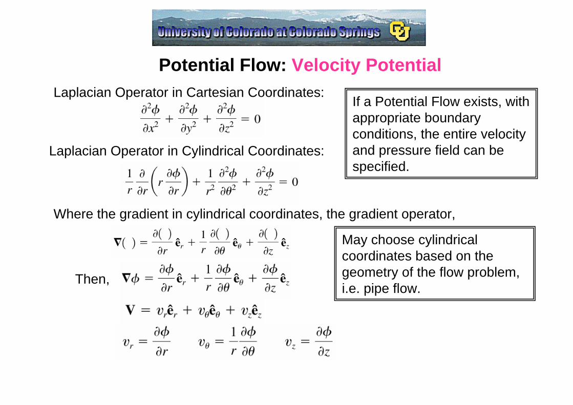
Potential Flow: Velocity PotentialLaplacian Operator in Cartesian Coordinates:

Laplacian Operator in Cylindrical Coordinates:

Where the gradient in cylindrical coordinates, the gradient operator,

Then,

May choose cylindrical coordinates based on the geometry of the flow problem, i.e. pipe flow.

If a Potential Flow exists, with appropriate boundary conditions, the entire velocity and pressure field can be specified.

Potential Flow: Plane Potential FlowsLaplace’s Equation is a Linear Partial Differential Equation, thus there are know theories for solving these equations.Furthermore, linear superposition of solutions is allowed:

where andare solutions to Laplace’s equation

For simplicity, we consider 2D (planar) flows:

Cartesian:

Cylindrical:

We note that the stream functions also exist for 2D planar flows

Cartesian:

Cylindrical:

Potential Flow: Plane Potential FlowsFor irrotational, planar flow:

Now substitute the stream function:

Then, Laplace’s Equation

For plane, irrotational flow, we use either the potential or the stream function, which both must satisfy Laplace’s equations in two dimensions.

Lines of constant Ψ are streamlines:

Now, the change of ϕ from one point (x, y) to a nearby point (x + dx, y + dy):

Along lines of constant φ we have dφ = 0,

0

Potential Flow: Plane Potential FlowsLines of constant φ are called equipotential lines.

The equipotential lines are orthogonal to lines of constant Ψ, streamlines where they intersect.

The flow net consists of a family of streamlines and equipotential lines.

The combination of streamlines and equipotential lines are used to visualize a graphical flow situation.

The velocity is inversely proportional to the spacing between streamlines.

Velocity increases along this streamline.

Velocity decreases along this streamline.

Potential Flow: Uniform FlowThe simplest plane potential flow is a uniform flow in which the streamlines are all parallel to each other.Consider a uniform flow in the x-direction:

Integrate the two equations:

φ = Ux + f(y) + C

φ = f(x) + C

Matching the solution

C is an arbitrary constant, can be set to zero:Now for the stream function solution:

Integrating the two equations similar to above.

Potential Flow: Uniform FlowFor Uniform Flow in an Arbitrary direction, α:

Potential Flow: Source and Sink FlowSource/Sink Flow is a purely radial flow.

Fluid is flowing radially from a line through the origin perpendicular to the x-y plane.Let m be the volume rate emanating from the line (per unit length.Then, to satisfy mass conservation:

Since the flow is purely radial:

Now, the velocity potential can be obtained:

Integrate

0If m is positive, the flow is radially outward, source flow.If m is negative, the flow is radially inward, sink flow.

m is the strength of the source or sink!This potential flow does not exist at r = 0, the origin, because it is not a “real” flow, but can approximate flows.

Source Flow:

Potential Flow: Source and Sink Flow

0

Now, obtain the stream function for the flow:

Then, integrate to obtain the solution:

The streamlines are radial lines and the equipotentiallines are concentric circles centered about the origin:

φ lines

Ψ lines

Potential Flow: Vortex FlowIn vortex flow the streamlines are concentric circles, and the equipotentiallines are radial lines.

where K is a constant.

Solution:

The sign of K determines whether the flow rotates clockwise or counterclockwise.

In this case, ,The tangential velocity varies inversely with the distance from the origin. At the origin it encounters a singularity becoming infinite.

φ lines

Ψ lines

Potential Flow: Vortex FlowHow can a vortex flow be irrotational?

Rotation refers to the orientation of a fluid element and not the path followed by the element.

Irrotational Flow: Free Vortex Rotational Flow: Forced Vortex

Traveling from A to B, consider two sticks

Initially, sticks aligned, one in the flow direction, and the other perpendicular to the flow.As they move from A to B the perpendicular-aligned stick rotates clockwise, while the flow-aligned stick rotates counter clockwise.The average angular velocities cancel each other, thus, the flow is irrotational.

Irrotational Flow:

Velocity increases inward.

Velocity increases outward.

Rotational Flow: Rigid Body RotationInitially, sticks aligned, one in the flow direction, and the other perpendicular to the flow.

As they move from A to B they sticks move in a rigid body motion, and thus the flow is rotational.

i.e., water draining from a bathtub

i.e., a rotating tank filled with fluid

Potential Flow: Vortex FlowA combined vortex flow is one in which there is a forced vortex at the core, and a free vortex outside the core.

A Hurricane is approximately a combined vortex

Circulation is a quantity associated with vortex flow. It is defined as the line integral of the tangential component of the velocity taken around a closed curve in the flow field.

For irrotational flow the circulation is generally zero.

Potential Flow: Vortex Flow

However, if there are singularities in the flow, the circulation is not zero if the closed curve includes the singularity.

For the free vortex:

The circulation is non-zero and constant for the free vortex:The velocity potential and the stream function can be rewritten in terms of the circulation:

An example in which the closed surface circulation will be zero:

Beaker Vortex:

Potential Flow: Doublet FlowCombination of a Equal Source and Sink Pair:

Rearrange and take tangent,

Note, the following:

Substituting the above expressions,

and

Then,

If a is small, then tangent of angle is approximated by the angle:

Potential Flow: Doublet Flow

Now, we obtain the doublet flow by letting the source and sink approach one another, and letting the strength increase.

K is the strength of the doublet, and is equal to ma/π.

is then constant.

The corresponding velocity potential then is the following:

Streamlines of a Doublet:

Potential Flow: Summary of Basic Flows

Potential Flow: Superposition of Basic Flows

Because Potential Flows are governed by linear partial differential equations, the solutions can be combined in superposition.

Any streamline in an inviscid flow acts as solid boundary, such that there is no flow through the boundary or streamline.

Thus, some of the basic velocity potentials or stream functions can be combined to yield a streamline that represents a particular body shape.

The superposition representing a body can lead to describing the flow around the body in detail.

Superposition of Potential Flows: Rankine Half-BodyThe Rankine Half-Body is a combination of a source and a uniform flow.

Stream Function (cylindrical coordinates):

Potential Function (cylindrical coordinates):

There will be a stagnation point, somewhere along the negative x-axis where the source and uniform flow cancel (θ = π):

For the source: For the uniform flow:

Evaluate the radial velocity:

θcosUvr =For θ = π, Uvr =

Then for a stagnation point, at some r = -b, θ = π:

π2mvr −= and

Superposition of Potential Flows: Rankine Half-BodyNow, the stagnation streamline can be defined by evaluating ψ at r = b, and θ = π .

Now, we note that m/2 = πbU, so following this constant streamline gives the outline of the body:

Then, describes the half-body outline.

So, the source and uniform can be used to describe an aerodynamic body.

The other streamlines can be obtained by setting ψ constant and plotting:Half-Body:

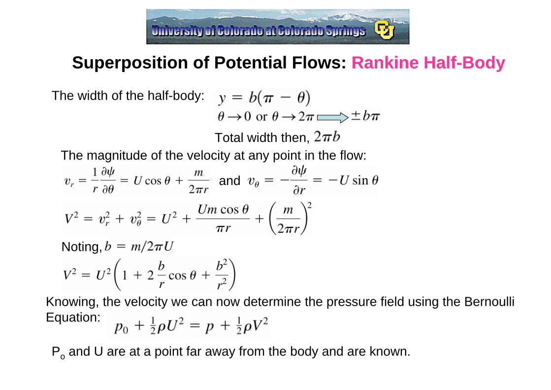
Superposition of Potential Flows: Rankine Half-Body

The width of the half-body:

Total width then, The magnitude of the velocity at any point in the flow:

Noting,

and

Knowing, the velocity we can now determine the pressure field using the Bernoulli Equation:

Po and U are at a point far away from the body and are known.

Superposition of Potential Flows: Rankine Half-BodyNotes on this type of flow:

• Provides useful information about the flow in the front part of streamlined body.• A practical example is a bridge pier or a strut placed in a uniform stream• In a potential flow the tangent velocity is not zero at a boundary, it “slips”• The flow slips due to a lack of viscosity (an approximation result).• At the boundary, the flow is not properly represented for a “real” flow.• Outside the boundary layer, the flow is a reasonable representation.• The pressure at the boundary is reasonably approximated with potential flow.• The boundary layer is to thin to cause much pressure variation.

Superposition of Potential Flows: Rankine OvalRankine Ovals are the combination a source, a sink and a uniform flow, producing a closed body.

Some equations describing the flow: The body half-length

The body half-width

“Iterative”

Potential and Stream Function

Superposition of Potential Flows: Rankine OvalNotes on this type of flow:

• Provides useful information about the flow about a streamlined body.• At the boundary, the flow is not properly represented for a “real” flow.• Outside the boundary layer, the flow is a reasonable representation.• The pressure at the boundary is reasonably approximated with potential flow.• Only the pressure on the front of the body is accurate though.• Pressure outside the boundary is reasonably approximated.

Superposition of Potential Flows: Flow Around a Circular CylinderCombines a uniform flow and a doublet flow:

and

Then require that the stream function is constant for r = a, where a is the radius of the circular cylinder:

K = Ua2

Then, and

Then the velocity components:

Superposition of Potential Flows: Flow Around a Circular Cylinder

At the surface of the cylinder (r = a):

The maximum velocity occurs at the top and bottom of the cylinder, magnitude of 2U.

Superposition of Potential Flows: Flow Around a Circular Cylinder

Pressure distribution on a circular cylinder found with the Bernoulli equation

Then substituting for the surface velocity:

Theoretical and experimental agree well on the front of the cylinder.

Flow separation on the back-half in the real flow due to viscous effects causes differences between the theory and experiment.

Superposition of Potential Flows: Flow Around a Circular Cylinder

The resultant force per unit force acting on the cylinder can be determined by integrating the pressure over the surface (equate to lift and drag).

(Drag)

(Lift)

Substituting, Evaluating the integrals:Both drag and lift are predicted to be zero on fixed cylinder in a uniform flow?Mathematically, this makes sense since the pressure distribution is symmetric about cylinder, ahowever, in practice/experiment we see substantial drag on a circular cylinder (d’Alembert’s Paradox, 1717-1783).

Viscosity in real flows is the Culprit Again!

Jean le Rondd’Alembert(1717-1783)

Viscous Flows: Surface Stress TermsNow, we allow viscosity effects for a Newtonian Fluid:

Normal Stresses: Shear Stresses:

Cylindrical Coordinates:

Cartesian Coordinates:

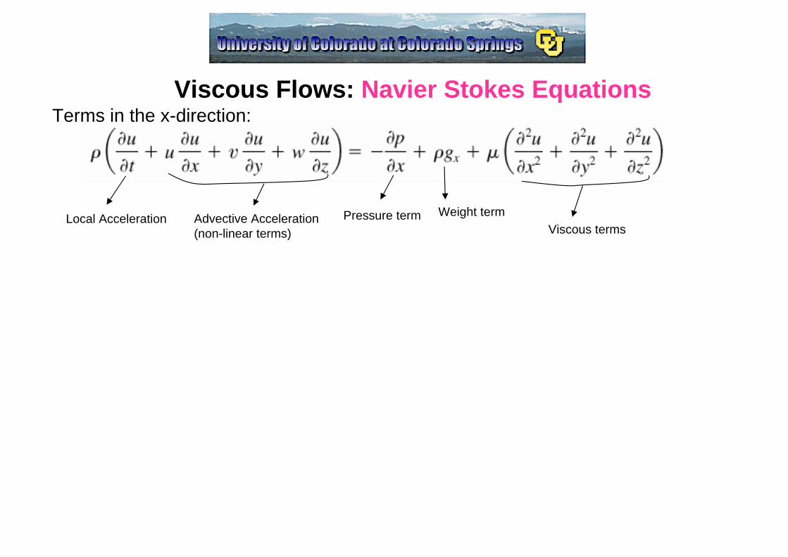
Viscous Flows: Navier-Stokes Equations

Now plugging the stresses into the differential equations of motion for incompressible flow give Navier-Stokes Equations:

French Mathematician, L. M. H. Navier (1758-1836) and English Mathematician Sir G. G. Stokes (1819-1903) formulated the Navier-Stokes Equations by including viscous effects in the equations of motion.

L. M. H. Navier(1758-1836)

Sir G. G. Stokes (1819-1903)

(x –direction)

Viscous Flows: Navier Stokes Equations

Local Acceleration Advective Acceleration(non-linear terms)

Pressure term Weight termViscous terms

Terms in the x-direction:

Viscous Flows: Navier-Stokes Equations

The governing equations can be written in cylindrical coordinates as well:

(r-direction)

Viscous Flows: Navier-Stokes Equations

There are very few exact solutions to Navier-Stokes Equations, maybe a total of 80 that fall into 8 categories. The Navier-Stokes equations are highly non-linear and are difficult to solve.

Some “simple” exact solutions presented in the text are the following:

1. Steady, Laminar Flow Between Fixed Parallel Plates2. Couette Flow3. Steady, Laminar Flow in Circular Tubes4. Steady, Axial Laminar Flow in an Annulus

Viscous Flows: Exact Solutions/Parallel Plate Flow

Assumptions:Plates are infiniteThe flow is steady and laminarFluid flows in the x-direction onlyu=u(y) only, v and w = 0

Navier-Stokes Equations Simplify Considerably:

Applying Boundary conditions (no-slip conditions at y = ± h) and solve:

The pressure gradient must be specified and is typically constant in this flow! The sign is negative.

(Integrate Twice)“No-Slip”:

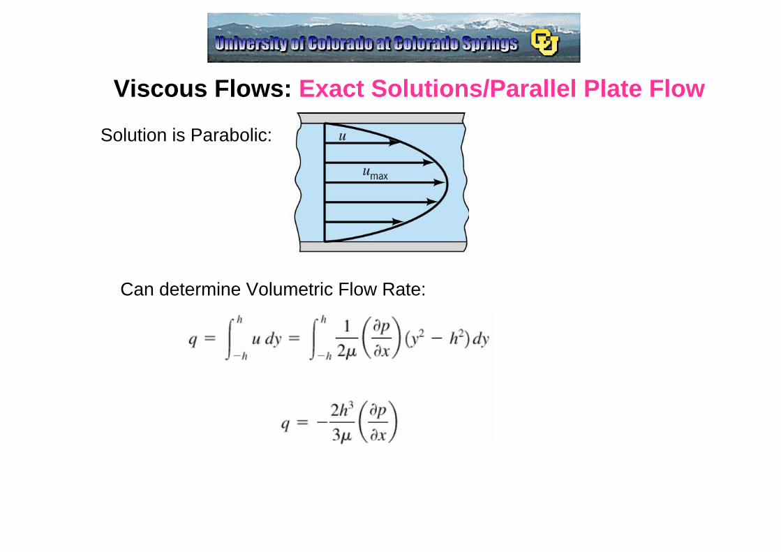
Viscous Flows: Exact Solutions/Parallel Plate Flow

Solution is Parabolic:

Can determine Volumetric Flow Rate:

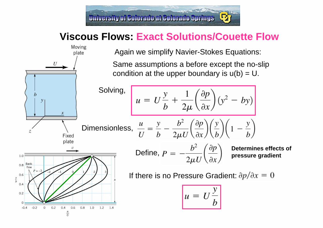
Viscous Flows: Exact Solutions/Couette FlowAgain we simplify Navier-Stokes Equations:Same assumptions a before except the no-slip condition at the upper boundary is u(b) = U.

Solving,

If there is no Pressure Gradient:

Define, Determines effects of pressure gradient

Dimensionless,

Viscous Flows: Exact Solutions/Pipe FlowAssumptions:Steady Flow and Laminar FlowFlow is only in the z-directionvz = f(r)

Simplifying the Navier-Stokes Equation in Cylindrical Coordinates:Solving the equations with the no slip conditions applied at r = R (the walls of the pipe).

“Parabolic Velocity Profile”

Viscous Flows: Exact Solutions/Pipe Flow

The volumetric flow rate:

The mean velocity:

Pressure drop per length of pipe:

The maximum velocity:

Non-Dimensional velocity profile:

For Laminar Flow:

Substituing Q,

“Laminar Flow”:

Computational Fluid Dynamics: Differential AnalysisGoverning Equations:

Navier-Stokes:

Continuity:

The above equations can not be solved for most practical problems with analytical methods so Computational Fluid Dynamics or experimental methods are employed.

The numerical methods employed are the following:1. Finite difference method2. Finite element (finite volume) method3. Boundary element method.

These methods provide a way of writing the governing equations in discrete form that can be analyzed with a digital computer.

Computational Fluid Dynamics: Finite ElementThese methods discretize the domain of the flow of interest (Finite Element Method Shown):

The discrete governing equations are solved in every element. This method often leads to 1000 to 10,000 elements with 50,000 equations or more that are solved.

“CFD Analysis”:

Computational Fluid Dynamics: Finite DifferenceThese methods discretize the domain of the flow of interest as well (Finite Difference Method Shown):

Finite Difference Mesh:

Comparison between Experiment and CFD Analysis:

Computational Fluid Dynamics: Pitfalls

Numerical Solutions can diverge or exhibit unstable wiggles.

Finer grids may cause instability in the solution rather than better results.

Large flow domains can be computationally intensive.

Turbulent flows have yet to be well described with CFD.

Some Example Problems