MAE 3130: Fluid MechanicsLecture 7: Differential Analysis/Part 1

Spring 2003Dr. Jason Roney

Mechanical and Aerospace Engineering

Outline• Introduction• Kinematics Review• Conservation of Mass• Stream Function• Linear Momentum• Inviscid Flow• Examples

Differential Analysis: Introduction

• Some problems require more detailed analysis.• We apply the analysis to an infinitesimal control

volume or at a point.• The governing equations are differential equations

and provide detailed analysis.• Around only 80 exact solutions to the governing

differential equations.• We look to simplifying assumptions to solve the

equations.• Numerical methods provide another avenue for

solution (Computational Fluid Dynamics)

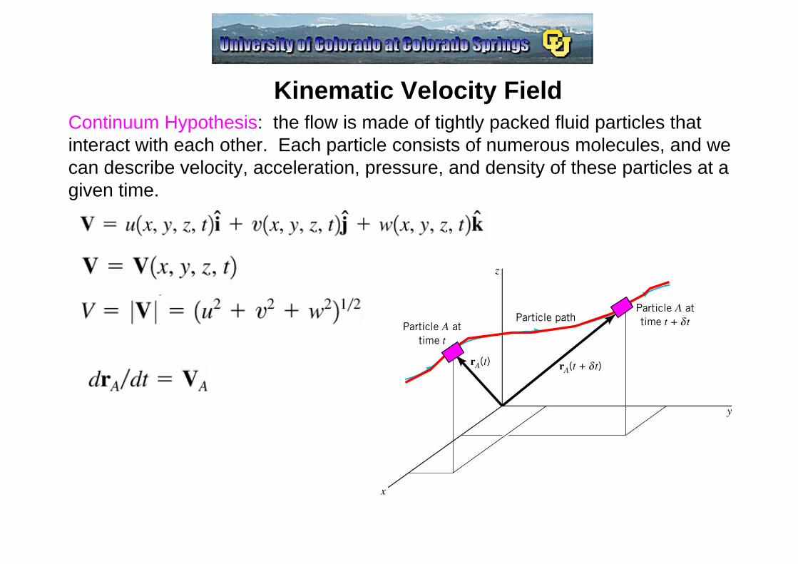
Kinematic Velocity FieldContinuum Hypothesis: the flow is made of tightly packed fluid particles that interact with each other. Each particle consists of numerous molecules, and we can describe velocity, acceleration, pressure, and density of these particles at a given time.

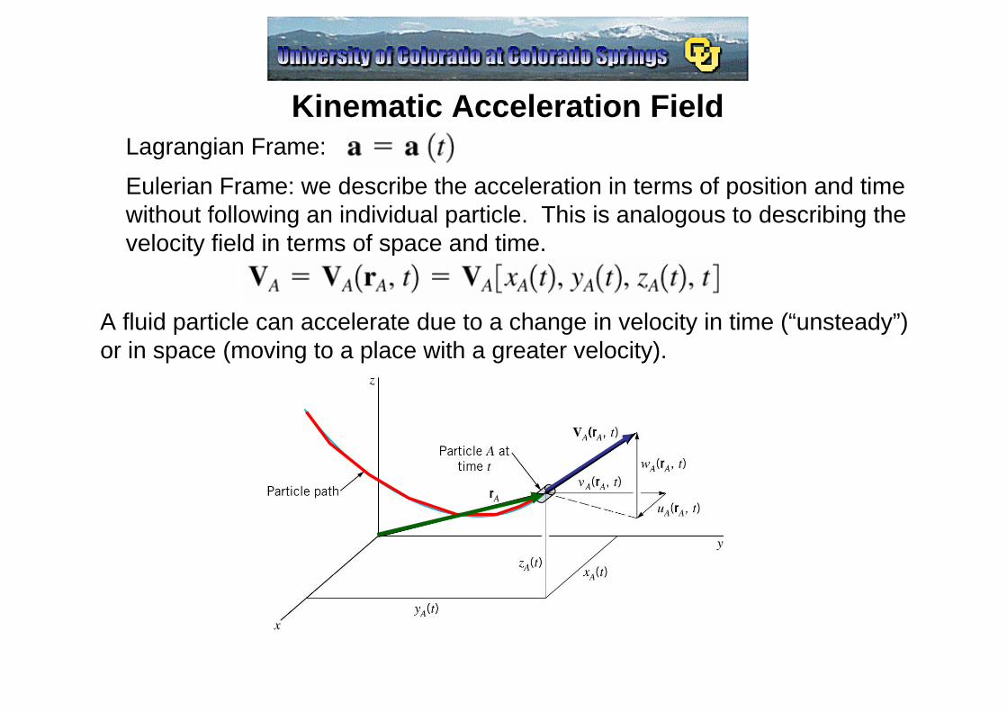
Kinematic Acceleration FieldLagrangian Frame:

Eulerian Frame: we describe the acceleration in terms of position and time without following an individual particle. This is analogous to describing the velocity field in terms of space and time.

A fluid particle can accelerate due to a change in velocity in time (“unsteady”) or in space (moving to a place with a greater velocity).

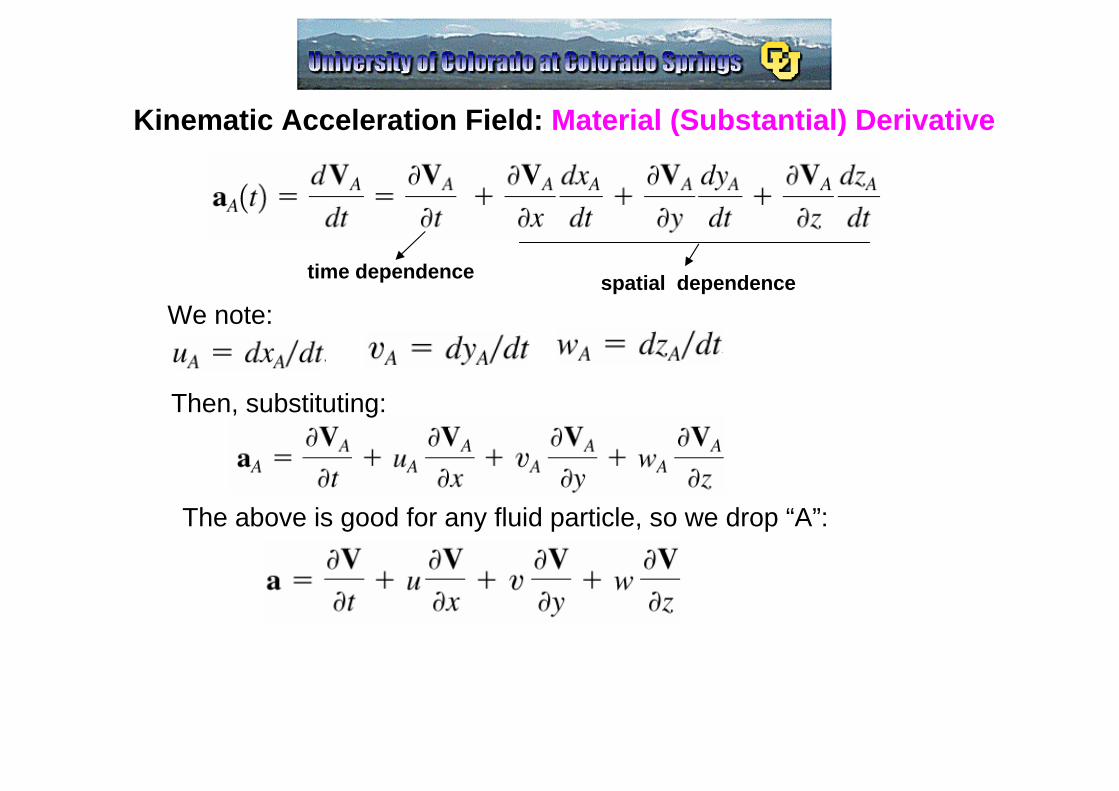
Kinematic Acceleration Field: Material (Substantial) Derivative

time dependence spatial dependenceWe note:

Then, substituting:

The above is good for any fluid particle, so we drop “A”:

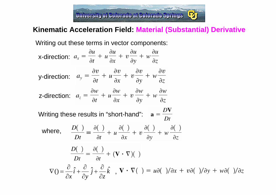
Kinematic Acceleration Field: Material (Substantial) Derivative

Writing out these terms in vector components:

x-direction:

y-direction:

z-direction:

Writing these results in “short-hand”:

where,

kz

jy

ix

ˆˆˆ()∂∂

+∂∂

+∂∂

=∇ ,

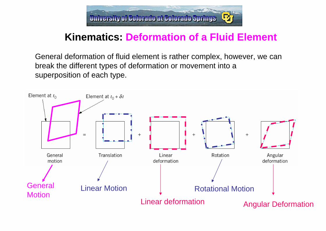
Kinematics: Deformation of a Fluid Element

General deformation of fluid element is rather complex, however, we can break the different types of deformation or movement into a superposition of each type.

Linear Motion Rotational Motion

Linear deformation Angular Deformation

General Motion

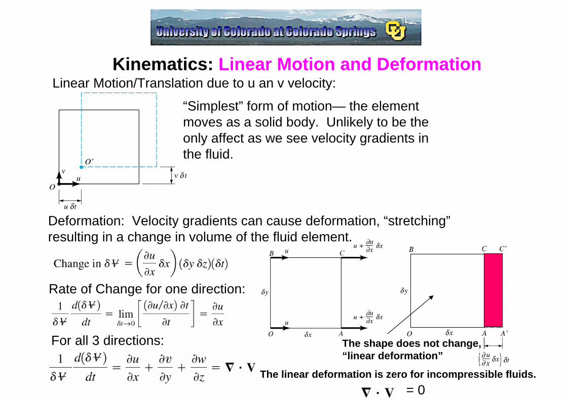
Kinematics: Linear Motion and DeformationLinear Motion/Translation due to u an v velocity:

“Simplest” form of motion— the element moves as a solid body. Unlikely to be the only affect as we see velocity gradients in the fluid.

Deformation: Velocity gradients can cause deformation, “stretching”resulting in a change in volume of the fluid element.

Rate of Change for one direction:

For all 3 directions: The shape does not change, “linear deformation”

The linear deformation is zero for incompressible fluids.= 0

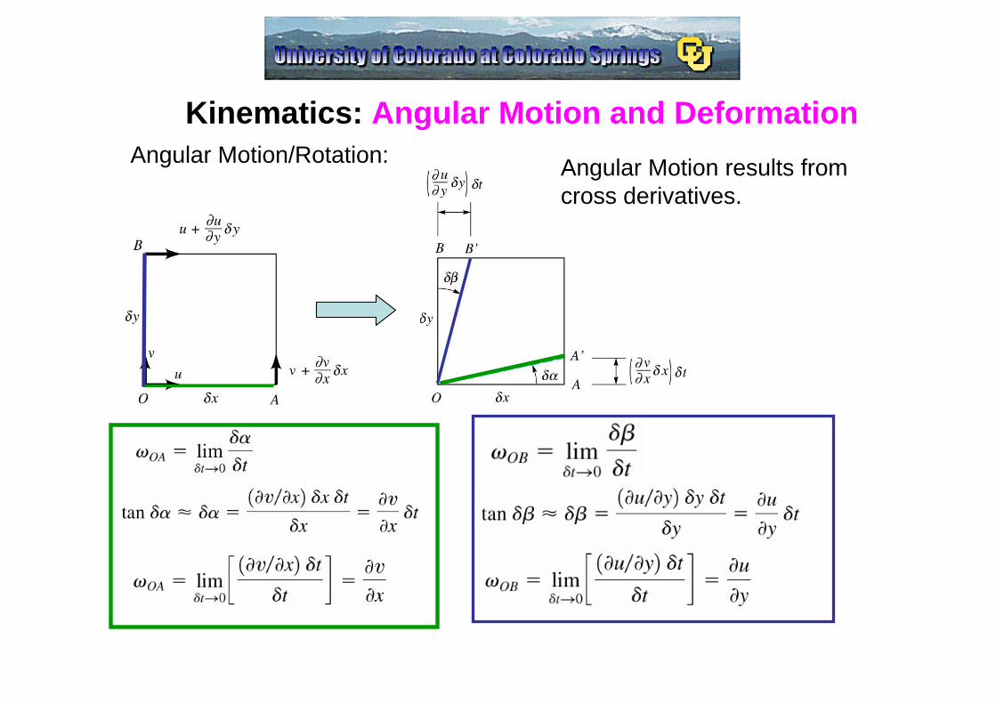
Kinematics: Angular Motion and DeformationAngular Motion/Rotation: Angular Motion results from

cross derivatives.

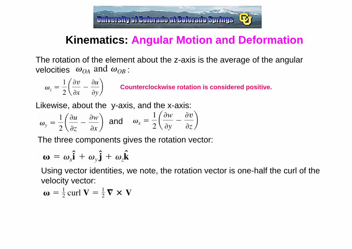
Kinematics: Angular Motion and DeformationThe rotation of the element about the z-axis is the average of the angular velocities :

Likewise, about the y-axis, and the x-axis:

Counterclockwise rotation is considered positive.

and

The three components gives the rotation vector:

Using vector identities, we note, the rotation vector is one-half the curl of the velocity vector:

Kinematics: Angular Motion and DeformationThe definition, then of the vector operation is the following:

The vorticity is twice the angular rotation:

Vorticity is used to describe the rotational characteristics of a fluid.

The fluid only rotates as and undeformed block when ,otherwise, the rotation also deforms the body.

If , then there is no rotation, and the flow is said to be irrotational.

Island Rotation:

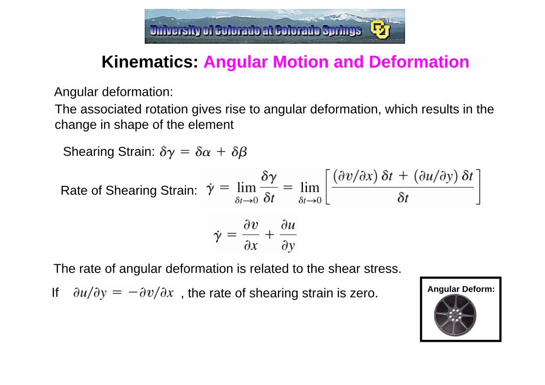
Kinematics: Angular Motion and DeformationAngular deformation:The associated rotation gives rise to angular deformation, which results in the change in shape of the element

Shearing Strain:

Rate of Shearing Strain:

If , the rate of shearing strain is zero.

The rate of angular deformation is related to the shear stress.Angular Deform:

Conservation of Mass: Cartesian CoordinatesSystem: Control Volume:

Now apply to an infinitesimal control volume:

For an infinitesimal control volume:

Now, we look at the mass flux in the x-direction:

Out: In:

Conservation of Mass: Cartesian Coordinates

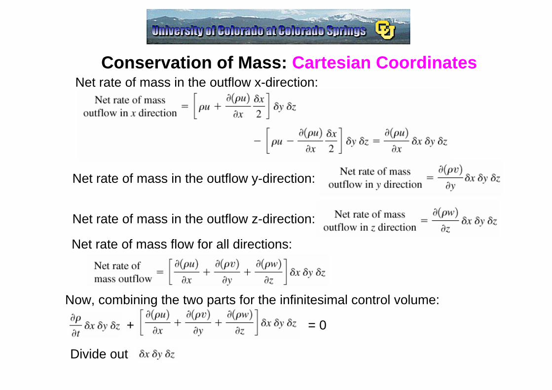
Net rate of mass in the outflow y-direction:

Net rate of mass in the outflow z-direction:

Net rate of mass in the outflow x-direction:

Net rate of mass flow for all directions:

+

Now, combining the two parts for the infinitesimal control volume:

= 0

Divide out

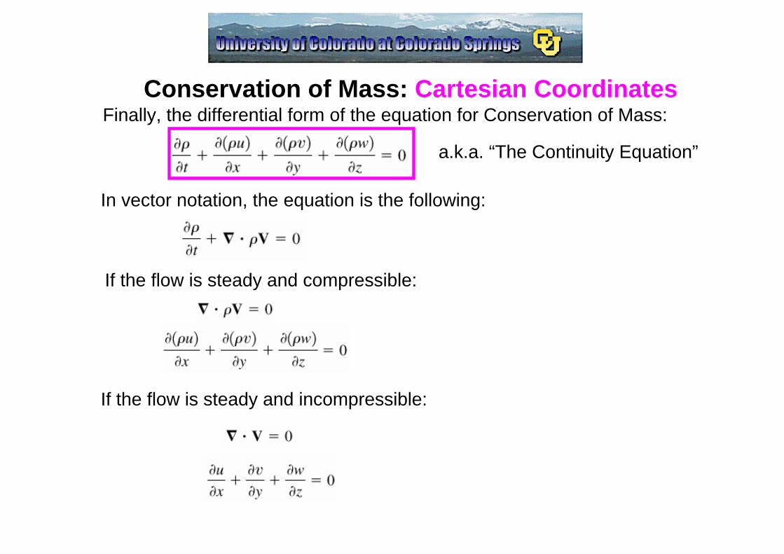
Conservation of Mass: Cartesian CoordinatesFinally, the differential form of the equation for Conservation of Mass:

a.k.a. “The Continuity Equation”

In vector notation, the equation is the following:

If the flow is steady and compressible:

If the flow is steady and incompressible:

Conservation of Mass: Cylindrical-Polar Coordinates

If the flow is steady and compressible:

If the flow is steady and incompressible:

Conservation of Mass: Stream FunctionsStream Functions are defined for steady, incompressible, two-dimensional flow.

Continuity:

Then, we define the stream functions as follows:

Now, substitute the stream function into continuity:

It satisfies the continuity condition.

The slope at any point along a streamline:

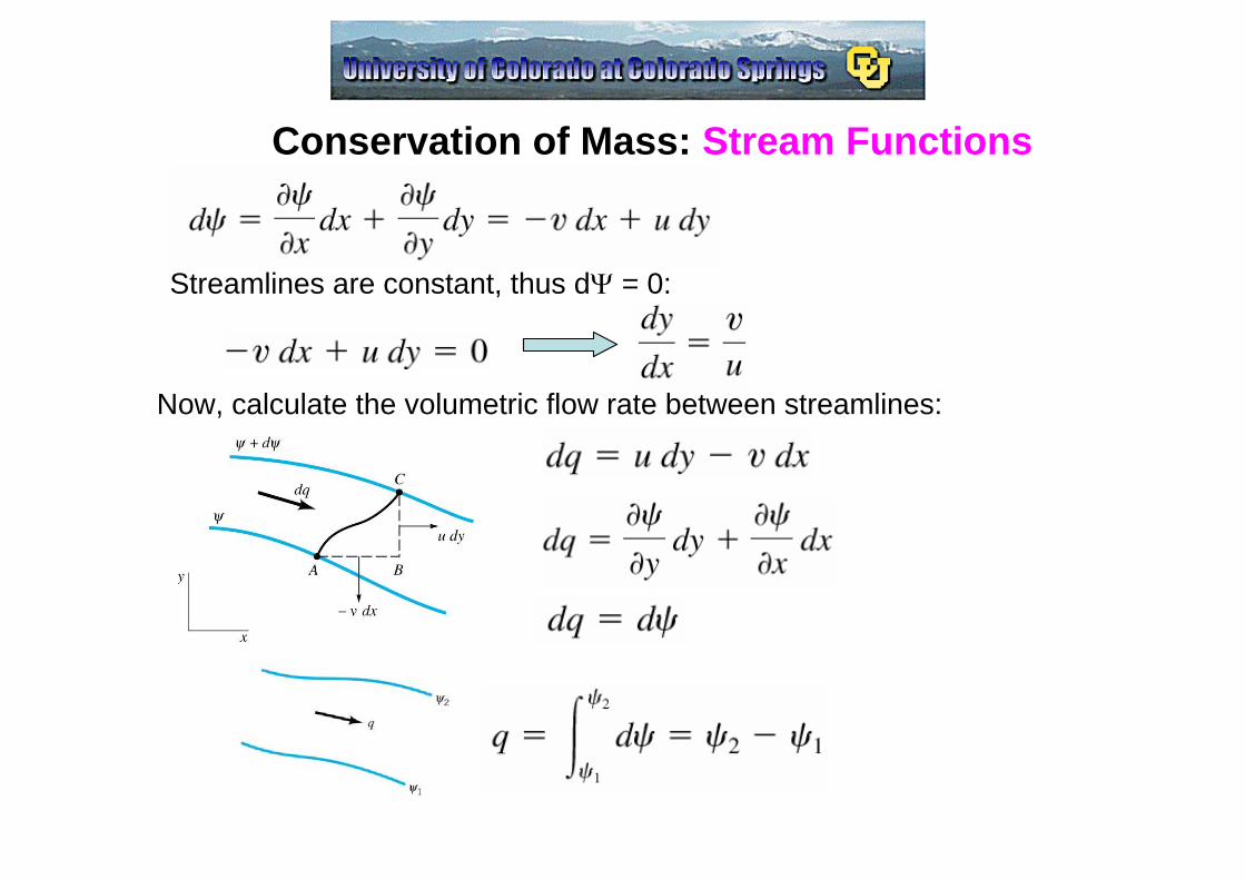
Conservation of Mass: Stream Functions

Streamlines are constant, thus dΨ = 0:

Now, calculate the volumetric flow rate between streamlines:

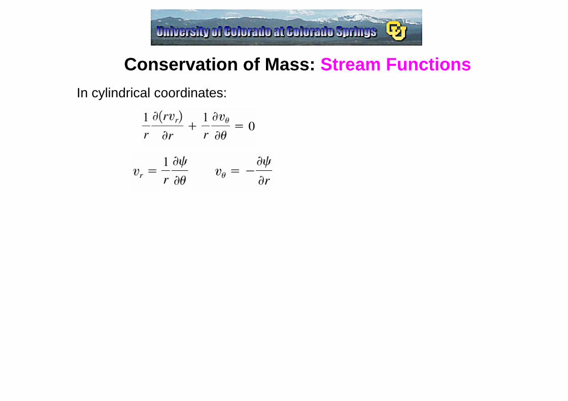
Conservation of Mass: Stream FunctionsIn cylindrical coordinates:

Conservation of Linear MomentumP is linear momentum,System:

Control Volume:

We could apply either approach to find the differential form. It turns out the System approach is better as we don’t bound the mass, and allow a differential mass.

By system approach, δm is constant.

If we apply the control volume approach to an infinitesimal control volume, we would end up with the same result.

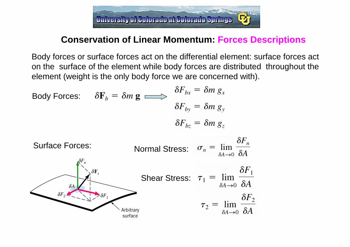
Conservation of Linear Momentum: Forces Descriptions

Body forces or surface forces act on the differential element: surface forces act on the surface of the element while body forces are distributed throughout the element (weight is the only body force we are concerned with).

Body Forces:

Surface Forces: Normal Stress:

Shear Stress:

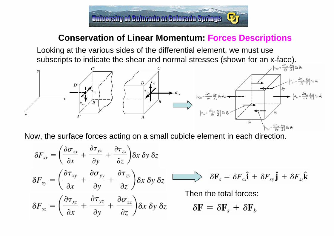
Conservation of Linear Momentum: Forces DescriptionsLooking at the various sides of the differential element, we must use subscripts to indicate the shear and normal stresses (shown for an x-face).

Now, the surface forces acting on a small cubicle element in each direction.

Then the total forces:

Conservation of Linear Momentum: Equations of Motion

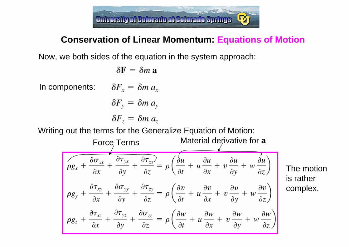
Now, we both sides of the equation in the system approach:

In components:

Writing out the terms for the Generalize Equation of Motion:Material derivative for aForce Terms

The motion is rather complex.

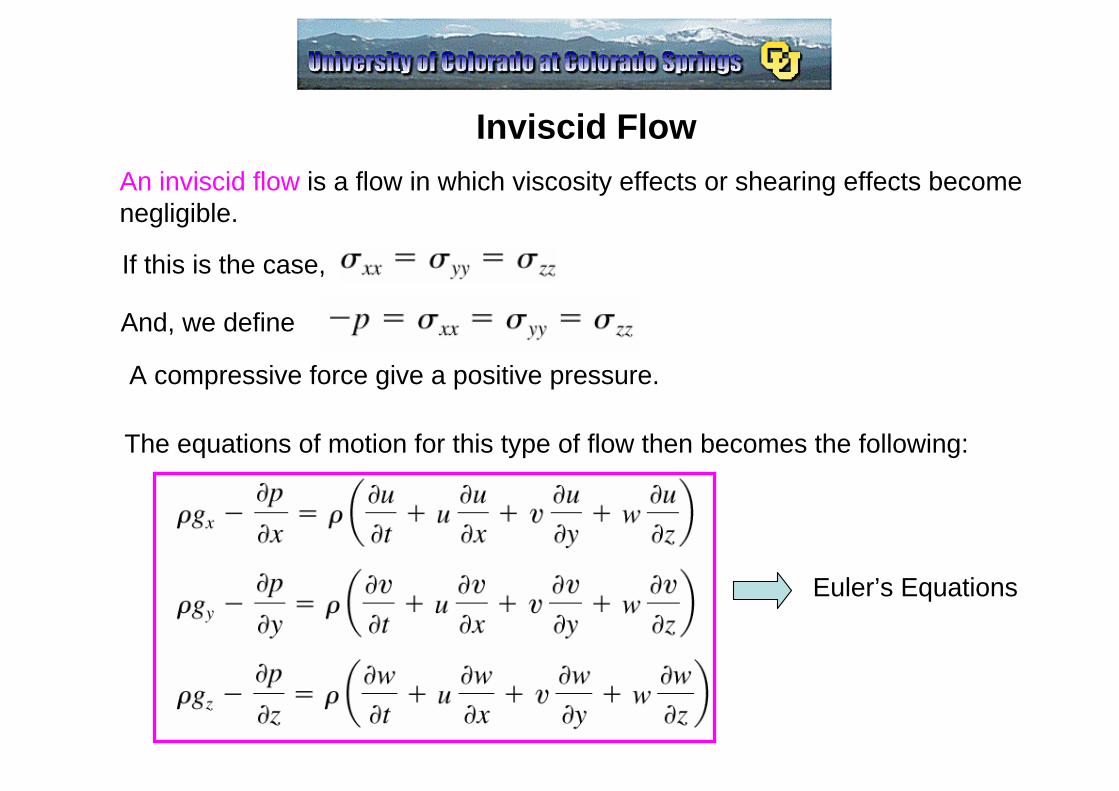
Inviscid FlowAn inviscid flow is a flow in which viscosity effects or shearing effects becomenegligible.

If this is the case,

And, we define

A compressive force give a positive pressure.

The equations of motion for this type of flow then becomes the following:

Euler’s Equations

Inviscid Flow: Euler’s Equations

Leonhard Euler(1707 – 1783)

Famous Swiss mathematician who pioneered work on the relationship between pressure and flow.

In vector notation Euler’s Equation:

The above equation, though simpler than the generalized equations, are still highly non-linear partial differential equations:

There is no general method of solving these equations for an analytical solution.

The Euler’s equation, for special situations can lead to some useful information about inviscid flow fields.

Inviscid Flow: Bernoulli Equation

Daniel Bernoulli(1700-1782)

Earlier, we derived the Bernoulli Equation from a direct application of Newton’s Second Law applied to a fluid particle along a streamline.

Now, we derive the equation from the Euler Equation

First assume steady state:

Select, the vertical direction as “up”, opposite gravity:

Use the vector identity:

Now, rewriting the Euler Equation:

Rearrange:

Inviscid Flow: Bernoulli EquationNow, take the dot product with the differential length ds along a streamline:

ds and V are parrallel, , is perpendicular to V, and thus to ds.

We note,

Now, combining the terms:

Integrate:

Then,1) Inviscid flow2) Steady flow3) Incompressible flow4) Along a streamline

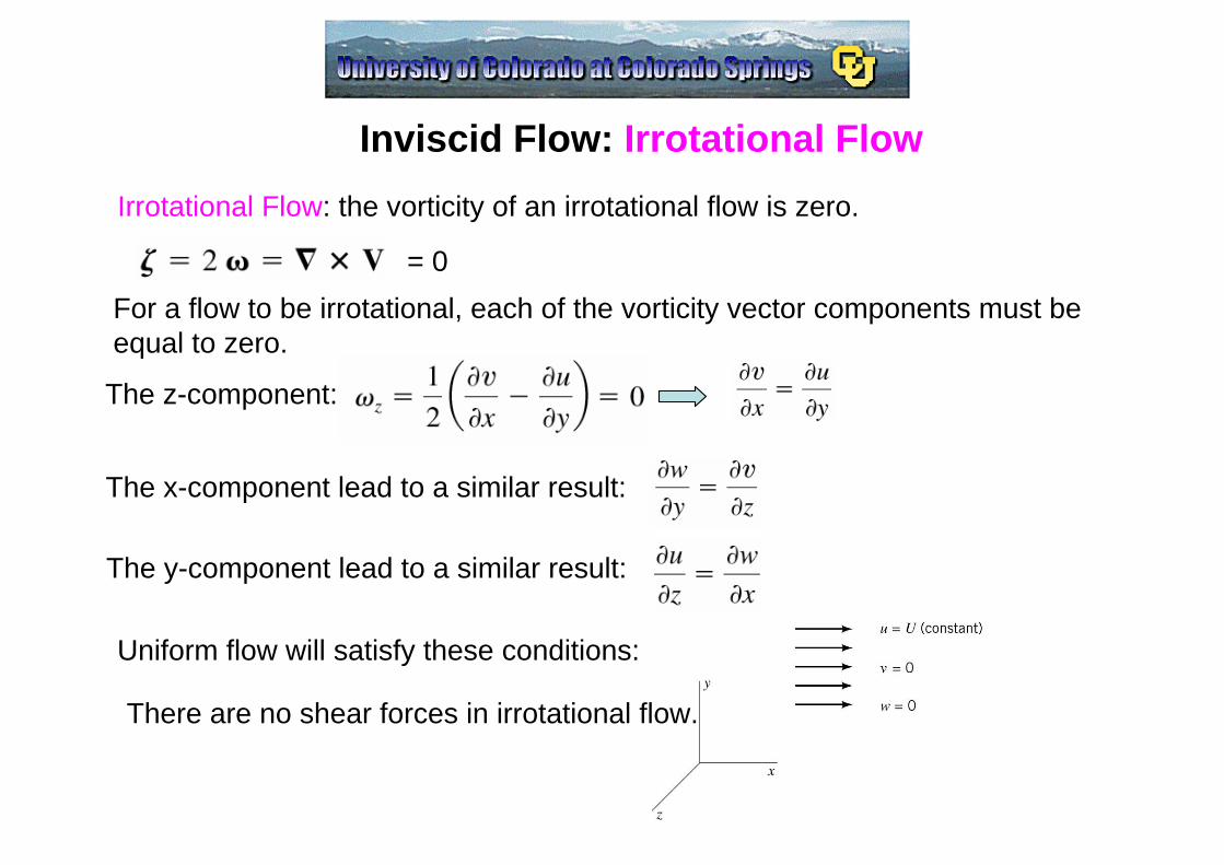
Inviscid Flow: Irrotational FlowIrrotational Flow: the vorticity of an irrotational flow is zero.

= 0For a flow to be irrotational, each of the vorticity vector components must be equal to zero.

The z-component:

The x-component lead to a similar result:

The y-component lead to a similar result:

Uniform flow will satisfy these conditions:

There are no shear forces in irrotational flow.

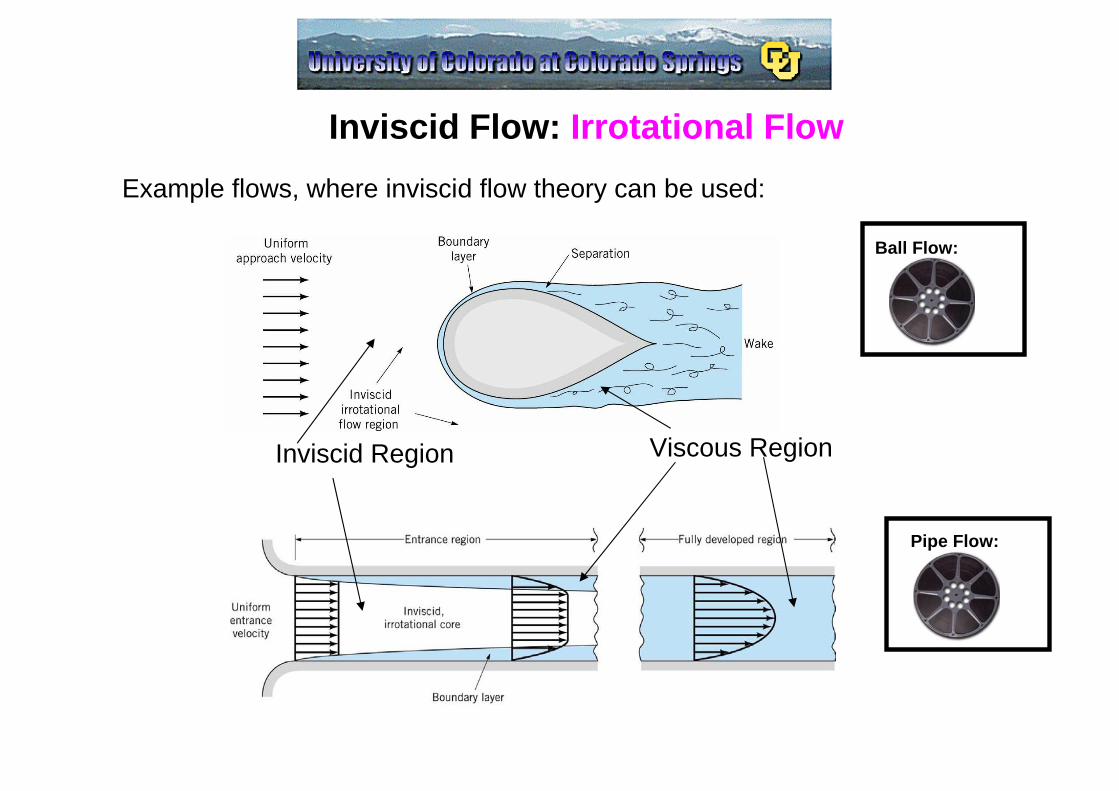
Inviscid Flow: Irrotational FlowExample flows, where inviscid flow theory can be used:

Viscous RegionInviscid Region

Ball Flow:

Pipe Flow:

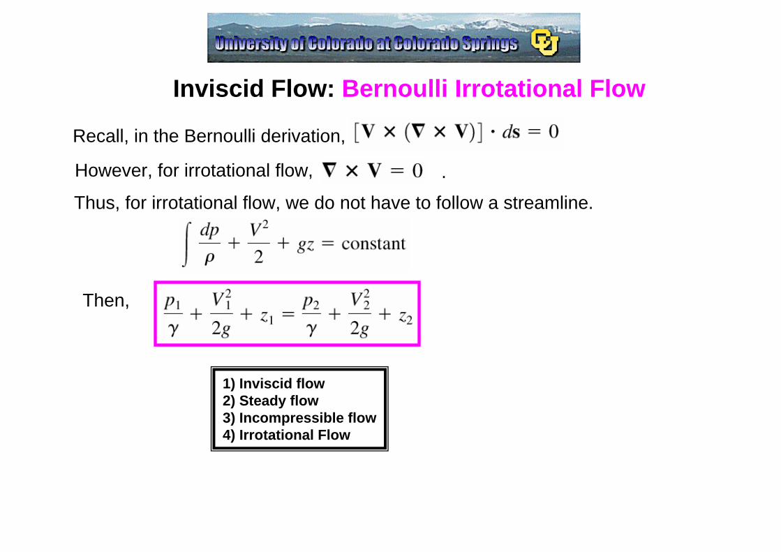
Inviscid Flow: Bernoulli Irrotational Flow

Recall, in the Bernoulli derivation,

However, for irrotational flow, .

Thus, for irrotational flow, we do not have to follow a streamline.

Then,

1) Inviscid flow2) Steady flow3) Incompressible flow4) Irrotational Flow

Some Example Problems