65

© The Ecological Society of America www.frontiersinecology.org

Many environmental problems cannot be adequatelyaddressed by viewing them through a single lens,

be it narrow or broad, because ecological interactionsoften cross boundaries of scale or levels of organization(Peters et al. 2011). Cross-scale interactions (CSIs) occurwhen driver and response variables in cause–effect rela-tionships operate at different characteristic spatial andtemporal scales, sometimes producing nonlinear patternsand dynamics (Carpenter and Turner 2000; Gundersonand Holling 2002; Peters et al. 2007). Understandingthese relationships is necessary to predict likely outcomesof alternative management strategies intended to miti-gate complex environmental problems (Miller et al. 2004;Peters et al. 2004; Tranvik et al. 2009). Because practi-

tioners of macrosystems ecology study such multi-scaledinteractions (Heffernan et al. 2014), this relatively newsubdiscipline of ecology includes the study of CSIs.

Macrosystems are made up of biological, geophysical,and sociocultural components that exhibit variation atthe scale of regions to continents (Heffernan et al. 2014).For simplicity, we use the term “macrosystems” here toinclude three dominant spatial “scales” (interpreted asspatial extents, but which can be interchanged with tem-poral extents), and we depict the potential interactionsthat make up a macrosystem as arrayed along a gradient ofcomplexity (Figure 1). Unidirectional interactions from abroader- to a finer-scaled driver or explanatory variable(green and orange arrows in Figure 1, a–d) and interac-tions that are bidirectional between two variables withina scale (black arrows in Figure 1, a–d) are perhaps the twomost studied interaction types.

There are a growing number of examples in the litera-ture describing the more complex relationships thatoccur when driver variables interact across scales (blueand red arrows in Figure 1, c and d). The first type of CSIoccurs when there is an interaction among driver vari-ables at different spatial scales that influences a focalresponse variable (Figure 1c; the CSI is depicted as a one-way arrow from the interaction between the driver vari-ables to the focal response variable). For instance, con-sider a case in which a broad-scale regional driver such asanthropogenic disturbance affects the degree to which alocal driver variable influences a focal response variable(eg Peters et al. 2007). Later sections of this paper presenta case study documenting this type of CSI betweenregional agriculture and wetland patches connected toand affecting nutrient concentrations in a downstream

MACROSYSTEMS ECOLOGY

Cross-scale interactions: quantifying multi-scaled cause–effect relationships inmacrosystemsPatricia A Soranno1*, Kendra S Cheruvelil1,2, Edward G Bissell1, Mary T Bremigan1, John A Downing3,Carol E Fergus1, Christopher T Filstrup3, Emily N Henry1,4, Noah R Lottig5, Emily H Stanley6, Craig A Stow7,Pang-Ning Tan8, Tyler Wagner9, and Katherine E Webster10

Ecologists are increasingly discovering that ecological processes are made up of components that are multi-scaled in space and time. Some of the most complex of these processes are cross-scale interactions (CSIs), whichoccur when components interact across scales. When undetected, such interactions may cause errors in extrap-olation from one region to another. CSIs, particularly those that include a regional scaled component, have notbeen systematically investigated or even reported because of the challenges of acquiring data at sufficientlybroad spatial extents. We present an approach for quantifying CSIs and apply it to a case study investigatingone such interaction, between local and regional scaled land-use drivers of lake phosphorus. Ultimately, ourapproach for investigating CSIs can serve as a basis for efforts to understand a wide variety of multi-scaled prob-lems such as climate change, land-use/land-cover change, and invasive species.

Front Ecol Environ 2014; 12(1): 65–73, doi:10.1890/120366

In a nutshell:• To address many pressing environmental problems, scientists

need to study cause–effect relationships at both fine andbroad scales across time and space

• Driver variables that control ecological processes can interactacross scales, but large amounts of data collected from manyregions are needed to study the processes at broad scales

• We offer an approach for measuring these types of interac-tions using 2100 lakes in 35 regions in North America

• This approach can be used to measure interactions acrossscales for other systems, to study a range of research questions

1Department of Fisheries and Wildlife, Michigan State University, EastLansing, MI *(soranno@anr.msu.edu); 2Lyman Briggs College,Michigan State University, East Lansing, MI; 3Department of Ecology,Evolution, and Organismal Biology, Iowa State University, Ames, IA;4current address: Division of Outreach and Engagement, Oregon StateUniversity, Tillamook, OR; continued on p 73

Cross-scale interactions in macrosystems PA Soranno et al.

66

www.frontiersinecology.org © The Ecological Society of America

lake. Other examples include tropical forest gastropoddiversity being influenced by the interaction betweenbroad-scale hurricane-induced disturbance and fine-scalehistorical land use (Willig et al. 2007), and the interac-tions between broad-scale forest fragmentation and local-scaled habitat variables that prevent some Chilean birdspecies from responding to local features that are knownto affect bird abundance (Vergara and Armesto 2009).

A second type of CSI is defined by interactions betweentransport processes that link fine- and broad-scaledprocesses as described in Peters et al. (2007). This CSI isdepicted in Figure 1d as a two-way arrow between the CSIamong driver variables and the feedback from the focalresponse variable (referred to as cross-scale emergence inHeffernan et al. [2014]). For example, this type of CSIoccurs when fire within patches interacts with regionalheterogeneity and connectivity among forest patches toinfluence fire spread at broad scales, and even the climatesystem in the case of a very large fire (Peters et al. 2007).

Other cases of this kind of CSI are the propagation of fine-scaled land-use effects that influence regional climate(Pielke et al. 2007), and patch configuration in semi-aridgrazed catchments causing unexpected broad-scale sedi-ment loss that was not equivalent to the sum of the indi-vidual finer-scaled sediment losses (Ludwig et al. 2007).Failure to account for the CSIs present in each of theabove examples would result in a misunderstanding of thecontrolling factors regulating the focal response variable.

In this paper, we offer an approach that uses Bayesianhierarchical models to explicitly model the CSIs that aredepicted in Figure 1c as an interaction term between aregional and a local driver variable. We illustrate theapproach using 2100 north temperate lakes in which lakephosphorus (P) is the focal response variable, the localwatershed characteristics of each lake are the local drivervariables, and the characteristics of the 35 regions thatthe lakes are nested within are the regional driver vari-ables. We end with a discussion of how such results can be

Figure 1. A description of four types of cause–effect relationships between driver variables and response variables withinmacrosystems, ranging from the simplest (a), to the more complex (c and d), in which there are cross-scale interactions (CSIs). Forsimplicity, we depict three main spatial extents of a macrosystem: the “focal response variables” are the fine-scale processes thatecologists typically study, the “local driver variables” (orange boxes) are the variables that are measured at a coarser scale and thatinfluence the focal response variables, and finally the “regional driver variables” (green boxes) are measured at macroscales (sub-continental to continental scales in the range of 100s to 1000s of kilometers; Heffernan et al. 2014). The green and orange arrowsdepict the one-way effect of regional and local driver variables, respectively, on the focal response variable. We define “driver” variablein the most general case as any explanatory variable measured at any scale that directly influences a focal response variable. Realmacrosystems can include additional extents that may exhibit a combination of different interaction types influencing the focalresponse variables. Some components of the figure are modified from Peters et al. (2008).

PA Soranno et al. Cross-scale interactions in macrosystems

67

© The Ecological Society of America www.frontiersinecology.org

applied in a management or policy con-text.

n Steps to quantify CSIs amongdriver variables

CSIs can be quantified using thisapproach (Figure 2) for any macrosystemand set of multi-scaled drivers with thefollowing minimum requirements: (1)hypotheses of the important cause–effectrelationships linking multi-scaled drivervariables to focal response variables inthe macrosystem(s), (2) data on the focalresponse variables across broad spatialand/or temporal extents, and (3) data onthe multi-scaled and multi-thematic dri-ver variables of the macrosystem(s).With these components, one can test formulti-scaled relationships using appro-priate models. These steps are iterativeand many are not unique to the study ofmacrosystems or CSIs. However, forsome steps, particular challenges arisethat are a consequence of the multi-scaled scope of macrosystems ecologyresearch and may require tools orapproaches that have not been widelyused by ecologists (eg Levy et al. 2014).In addition, for almost all of the steps dis-cussed here, ecoinformatics (the use ofsoftware tools to manipulate, store, anddistribute ecological data) is integrallylinked in all aspects of the research, fromdatabase design and management to analytical operations,and ultimately to database documentation and sharing(Michener and Jones 2012; Rüegg et al. 2014).

Step 1: conceptual model

The first and most important step when quantifying CSIsamong drivers is to translate current understanding of themacrosystem and its important multi-scaled cause–effectrelationships into a conceptual model. We argue that this isone of the more challenging steps because it requires a solidworking understanding of macrosystems. Four key compo-nents of conceptual model development are: (1) identifyingthe relevant spatial and temporal extents and resolutions ofthe driver variables, (2) considering what types of CSIs areexpected, (3) determining whether relationships are likelyto be linear or nonlinear, and (4) identifying the criticalassumptions and uncertainties that may generate additionaltestable hypotheses (Figure 2). Our approach to quantifyingCSIs is iterative. The cause–effect relationships (includingCSIs) identified in this first step can be refined or newcause–effect relationships can be added during subsequentiterations and as new information becomes available.

Step 2: database design and development

Rarely are there preexisting databases that span the spatialand temporal extents necessary to conduct macrosystemsecological research. Therefore, these next steps includediscovering and acquiring datasets that are distributedacross space and time and integrating them into a multi-scaled, multi-thematic database. When more than a hand-ful of datasets are incorporated into a database, numerousecoinformatics challenges may arise (Michener and Jones2012; Rüegg et al. 2014). Essential steps in database devel-opment are to identify credible data sources, to performquality-assurance and quality-control checks, and to pro-duce detailed documentation in the form of metadata foreach dataset and the final integrated database (see Rüegget al. [2014] for further details).

Step 3: analytical approaches

The analytical steps begin with translating the conceptualmodel into a set of models that each represents competinghypotheses to be evaluated and compared (Burnham andAnderson 2002; Stow et al. 2009). Such models can take

Steps• Identify the relevant spatial and temporal scales of

the macrosystem• Identify the hypothesized types of cross-scale

interactions (CSI) that may exist (see Figure 1)• Identify which of the CSI and non-CSI

relationships are likely to be linear or nonlinear• Identify critical uncertainties

Steps• Identify and compile data sources• Summarize explanatory variables (ie drivers) at

multiple scales (eg local, regional, monthly, annual)• Integrate datasets across space, time, and theme,

accounting for differences in data resolution• Perform quality control of all datasets• Document metadata of all individual data sources

Steps• Translate candidate model(s) into BH models• Address the computational costs associated with

parameter estimation when using large datasets(~10 000s of observations)

• Fit BH models to quantify CSIs (Figure 1c) asinteraction terms between a regional and localdriver (or any two different scales)

• Assess implications of uncertainties in parametersand variables for making predictions and inferences

Figure 2. The three main steps used to quantify CSIs through a multi-thematic,multi-scaled database and Bayesian hierarchical models. We focus on the compilationof especially large and spatially distributed datasets to characterize the within- andacross-region heterogeneity in the study area by fitting region-varying models withsufficient data to support the models.

Cross-scale interactions in macrosystems PA Soranno et al.

68

www.frontiersinecology.org © The Ecological Society of America

many forms, including process, statistical, and/or simula-tion. For statistical modeling, the parameter estimationand model inference can be Bayesian or non-Bayesian.We present modeling steps using Bayesian hierarchicalmodels, which are well suited for analyzing multi-thematicand multi-scaled data (Qian et al. 2010) as well as dataacross broad spatial (and temporal) extents with variablesample sizes and associated with unbalanced samplingdesigns (Gelman and Hill 2007; Cressie et al. 2009).Hierarchical models allow model coefficients (eg slopesand intercepts) to vary by region, which provides an ele-gant way to measure one type of CSI (as depicted in Figure1c) by simultaneously modeling both the local-scale vari-ability in the response variable of interest and the variabil-ity in regional-scale coefficients. Here, we model a CSI asan interaction term between two driver variables mea-sured at different scales (eg orange and green boxes inFigure 1c) which influences the response variable in addi-tion to the individual effects of the two driver variables(in Figure 1c, this interaction is depicted by the bluecurved arrows; see below for further details).

Once a model or model set has been developed andestimated from the data, the ecological importance of theresulting parameter estimates and/or predictions is evalu-ated within the context of the hypotheses, the concep-tual and analytical model(s), and the degree of uncer-tainty in variables or parameters. In some cases, candidatemodels that are not computationally feasible will have tobe simplified. Once all the models have been evaluated,revisions to the conceptual model can be made and addi-tional models created and tested iteratively.

n Case study – understanding drivers of lakenutrients at subcontinental scales

Using lakes as model ecosystems to study CSIs

We illustrate the approach described above by modelinglake P concentrations at the subcontinental scale in 35

regions, using multi-scaled driver variables to test for ahypothesized CSI. There are strong conceptual and prac-tical reasons for focusing on lakes for macrosystems ecol-ogy research and specifically to study CSIs. First, lakes areinfluenced by multiple well-studied spatial extentsincluding the watershed, the lake network, and the fresh-water region (Figure 3), as well as multiple temporalextents including daily, seasonal, interannual, decadal,and centurial scales. Although the land–water boundaryof lakes is less functionally distinct than originallyassumed (Cole et al. 2002), the physical boundary of thelake shoreline does represent a shift from aquatic to non-aquatic habitats and therefore facilitates easy map-basedmeasurements of macrosystem variables across broad spa-tial extents. Second, as gathering points of water andnutrients, lakes integrate the effects of hydrologic, land-use, and climatic changes at a range of spatial and tempo-ral scales (Williamson et al. 2009). Third, a wealth of dataand knowledge exist for lakes, including single-scaledstudies that provide the possible mechanisms needed tounderstand how driver variables of lake nutrients mayinteract across scales. Fourth, a hierarchical conceptualframework, such as that found in landscape limnology, isneeded to understand the complex suite of driver vari-ables and possible CSIs that influence lake response vari-ables, such as nutrients (Soranno et al. 2010). Finally,lakes and their nutrients have the advantage that reliabledata, obtained by standard methods, are widely availableacross broad geographic and temporal extents and can beintegrated into a single database.

Does a CSI between regional agriculture and localwetland cover affect lake nutrient concentrations?

In many regions of the world, an increase in the amount ofagricultural land use directly around lakes (ie local scale)has been shown to increase aquatic P concentrations(Taranu and Gregory-Eaves 2008). However, the same can-not be said for the effect of local wetland cover on lake P

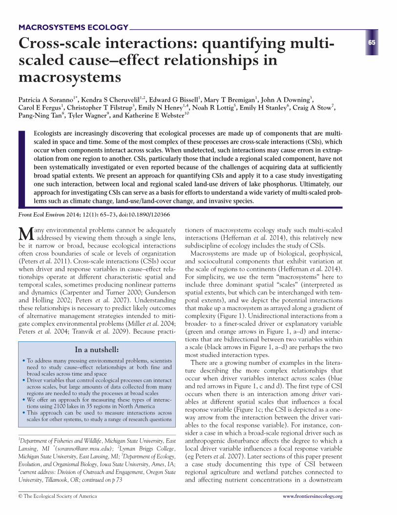
Figure 3. Images showing the different spatial extents that are relevant for multi-scaled studies of lakes, including (a) the lake and itswatershed, (b) the lake network, and (c) the freshwater region. The freshwater region classification that we use in this example isEcological Drainage Units (Higgins et al. 2005). There are many driver variables that can be quantified at each of these importantspatial extents (eg land cover, connectivity among freshwater ecosystems and groundwater, geology, soils) based on the conceptualframework of landscape limnology (Soranno et al. 2010). Images from The National Map – Orthoimagery, US Geological Survey,http://nationalmap.gov/ortho.html.

(a) (b) (c)

PA Soranno et al. Cross-scale interactions in macrosystems

69

© The Ecological Society of America www.frontiersinecology.org

concentrations. Wetland cover surrounding lakeshas been found to both increase (Prepas et al.2001) and decrease (Weller et al. 1996) the con-centration of lake P, depending on the regionstudied. We hypothesized that these divergentrelationships could be explained by a CSI, inwhich regional agriculture (a measure of regionalanthropogenic disturbance) influences thedegree to which local wetlands affect lake P con-centrations. Regions dominated by agriculturealso have modified hydrological, nutrient, andmaterial connectivity that likely influence theeffect that local wetlands (many of which havealso been altered) have on downstream lakenutrients. Therefore, a lake in close spatial prox-imity to intensive agriculture (ie within its water-shed boundaries), in an otherwise “low agricul-ture” region, will be less affected by anthro-pogenic modifications overall (at both the localand regional scales) than a lake whose watershedand region both have intensive agriculture. The steps(and results) to test for the presence of this CSI, and itseffects on lake nutrients, are described as follows.

Step 1

Our conceptual model of the multi-scaled spatial drivervariables of lake total P is informed by the theory andconcepts of landscape limnology. Landscape limnologyviews lakes and other freshwater systems as one piece ofthe multi-scaled aquatic, terrestrial, and human land-scape mosaic (Soranno et al. 2010), all of which makesup the macrosystem. Using this framework and findings

from past studies, we identified the multi-scaled drivervariables that we hypothesized to affect the focalresponse variable, lake P. Our conceptual model of thelocal and regional features that were most likely to berelated to P (Figure 4a) included: lake depth (Taranu andGregory-Eaves 2008), the ratio of the watershed-to-lakearea (ie drainage ratio; Prepas et al. 2001), groundwaterpotential (Devito et al. 2000), local and regional agricul-ture (Taranu and Gregory-Eaves 2008), local urbancover (Frost et al. 2009), and the CSI between regionalagriculture and local wetland effects. Given the resultsfrom past studies, we did not expect the driver variables

Figure 4. The conceptual and analytical results of thecase study. (a) A conceptual model of the driver variablesfor the Bayesian hierarchical model, in which the focalresponse variable is lake P; the local driver variables are:local % wetland cover around the lake, lake depth (meandepth), drainage ratio (the ratio of watershed-to-lakearea), groundwater potential (measured as the %groundwater contribution to stream baseflow near thelakes), local % agriculture around the lake, and local %urban land around the lake; the CSI is an interactionterm between regional % agriculture and local % wetlandcover. The slope of the effect of local % wetland coverwas not different from zero, so is represented by a dashedline in this conceptual figure. The model is the type ofCSI depicted in Figure 1c. (b) The relationship betweenlocal % wetland cover and lake P, modeled for eachregion. Black lines represent region-specific relationshipsand the bold blue line is the population averagerelationship across all regions, which is not different fromzero. (c) The relationship between regional % agricultureand the 35 region-specific slopes. Solid circles are region-specific slope estimates, shown with the multilevelregression line, and dark- and light-gray shaded regionsare 95% and 80% credible intervals, respectively.

(a)

(b)

(c)

Local % wetland cover

Regional % agriculture

Cross-scale interactions in macrosystems PA Soranno et al.

70

www.frontiersinecology.org © The Ecological Society of America

to exhibit nonlinear relationships with the responsevariable.

Step 2

We compiled lake nutrient data for 2100 lakes across theMidwest and northeastern US into a single database(Figure 5). Data came from six state management agencies(Iowa, Wisconsin, Michigan, Ohio, New Hampshire, andMaine) that followed federally approved laboratory andfield protocols and represent single-point measures ofnutrients during summer stratification (individual datasetsare described in Webster et al. [2008] and Wagner et al.[2011]). We also gathered aquatic, terrestrial, and humanlandscape information from national-scale geographicinformation systems (GIS) datasets (eg NationalHydrography Dataset, National Land Cover Dataset) andintegrated them with the lake nutrient database.Landscape data were quantified at two spatial scales: localand regional. Local features were quantified within a 500-m buffer around lakes, a measure that is strongly correlatedwith landscape features in the watershed (Fergus et al.2011). Regional features were quantified within theEcological Drainage Unit, a regionalization framework

developed to classify freshwater ecosystems based onhydrologic, physiographic, and climatic features (Higginset al. 2005). This database captured sufficient spatial het-erogeneity in terms of P within and across the 35 regionsso we could address our multi-scaled research questions(Cheruvelil et al. 2013).

Step 3

We translated the conceptual model in Figure 4a into aBayesian hierarchical model. The response variable wasloge-transformed P concentration in 2100 lakes in the 35different regions (Figure 5). The driver variables were fea-tures measured at local, regional, or both scales (Figure4a), as well as an interaction term between local % wet-lands and regional % agriculture (ie the hypothesizedCSI). We hypothesized that the slope estimates from thelocal % wetland–lake P relationship would differ byregion and that regional % agriculture would explainsome of the variation in these slopes.

We found good evidence in support of the hypothe-sized CSI (Figure 4c). There was substantial variation inthe slopes of the relationship between local % wetlandsand P across the regions, with slopes that were either

Figure 5. Map of the lakes used in the case study, the boundaries of the 35 regions defined by Ecological Drainage Units. These regionsrange in area from 2800 to 49 000 km2 (mean: 18 500 km2; standard deviation: 10 300 km2). Lakes are shown as dots, with the colorrepresenting P concentration. The six states in the study area include Iowa, Wisconsin, Michigan, Ohio, New Hampshire, and Maine.

0 75 150 225 300 Kilometers

Total phosphorus (µg L–1)1–1010–2020–3030–100100–200200–300>300

State boundaries

Ecological Drainage Units

0 75 100 Kilometers

PA Soranno et al. Cross-scale interactions in macrosystems

positive, negative, or zero (Figure 4b). In regions withlow % agriculture, local wetlands were positively associ-ated with P; whereas, in regions with high % agricul-ture, local wetlands were negatively associated with P(Figure 4c). The differential effects of local % wetlandson P were not due to an interaction between local %agriculture and local % wetlands (CEF unpublisheddata); rather, it was the interaction across scales thatmattered (Figure 4c). Regional % agriculture accountedfor some of the variation in the wetland–P slope differ-ences across regions, with the 95% credible interval forthe CSI parameter in the model not overlapping zero(posterior mean = –1.19, 95% credible interval = –2.34,–0.02; 80% credible interval = –2.17, –0.22). This CSIbetween local wetlands and regional agriculture was lin-ear, as expected; the data show a linear relationshipbetween regional agriculture and the region-specificwetland–P slope (Figure 4c). If we had ignored theregional variation in this relationship, we would havedetected no effect of local wetlands on P because theoverall slope of the relationship across the entire datasetwas weak, with a 95% credible interval including zero(blue line in Figure 4b).

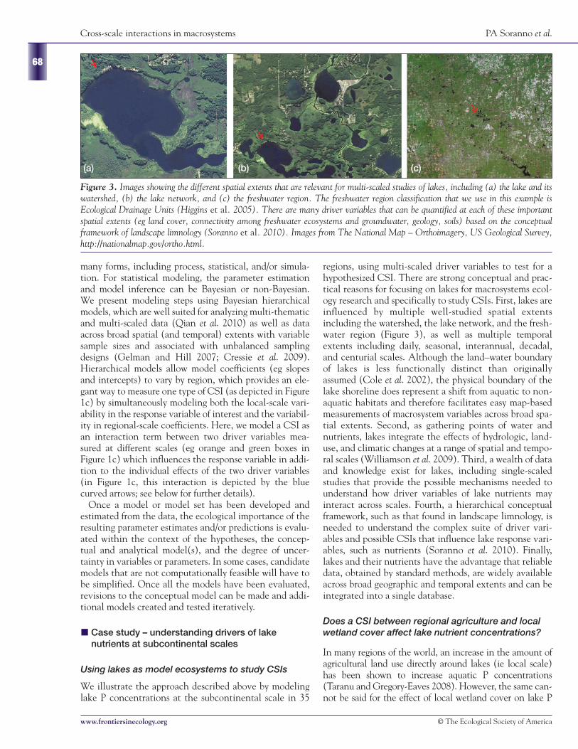
We can use these results to develop additional hypothe-ses to help explain variations in P and improve our under-standing of these macrosystems. One interpretation ofthe results is that in regional settings dominated by agri-culture, wetlands act as a P “sink” on the landscape,retaining excess P before it enters lakes (Figure 6).However, the spatial arrangement and hydrological con-nectivity of wetlands in the watershed are likely to beimportant at the local scale. Therefore, future workshould examine the importance of connectivity in wet-land–P relationships by developing freshwater connectiv-ity metrics that better capture mechanistic P–water trans-port relationships at the local scale. For instance, wehypothesize that freshwater connectivity differs inregions with different levels of human disturbance andcould be important in better understanding fine-scaledrelationships across regions.

n Applying CSI research to management and policy

As macrosystem ecologists identify and quantify interac-tions underlying environmental problems, many of whichare multi-scaled, they will be able to play an increasinglyimportant role in developing sound policy and manage-ment strategies (Carpenter and Turner 2000; Peters et al.2008). By identifying the most important environmentalgradients and CSIs driving valued ecosystem responsevariables (as per steps described in Peters et al. [2008]),researchers can, by logical extension, determine in whatcontexts modeled relationships can be translated fromone region or time period to another. Improved under-standing of CSIs may facilitate better identification ofindividual ecosystems and regions that are particularlyvulnerable to human impacts, and therefore might needstronger protection or different management approachesthan less vulnerable systems or regions. Finally, becauseknowledge of CSIs defines the spatial and temporalbounds within which particular modeled relationshipsapply, management agencies can strive to align policywith the spatial/temporal structures defined by CSIs.

Our results demonstrate how a CSI between regionalland use and local wetlands affects lake water quality,showing that one-size-fits-all management decisions willoften be ineffective. Such an approach inappropriatelyassumes that cause–effect relationships between systemresponse variables and driver variables are the same acrossbroad geographic extents and through time. Our exampleshows that local understanding (eg identifying the rela-tionship between local wetlands and lake nutrients) anddecisions within a region (eg which wetlands to prioritizefor protection) can be informed by incorporatingregional-scale attributes (eg regional agricultural landuse) into a multi-scaled framework that uses informationfrom a broad geographic area.

Looking to the future, we anticipate many managementscenarios that will benefit from considering environmen-tal problems at broader spatial (and temporal) extentsthan have conventionally been used by researchers and

71

© The Ecological Society of America www.frontiersinecology.org

Figure 6. Images from our study area showing the different landscape settings of (a) low and (b) high regional % agriculture. Imagesfrom The National Map – Orthoimagery, US Geological Survey, http://nationalmap.gov/ortho.html.

(a) (b)

Cross-scale interactions in macrosystems PA Soranno et al.

resource managers. Although criteria for managing fresh-water nutrients in the US are mainly determined at thestate level, results from our six-state analysis highlight theusefulness of considering extents beyond individual state(political) boundaries. For instance, P within Michiganlakes, one of the states included in our study, varies rela-tively little among regions (Cheruvelil et al. 2008); yetacross multiple states, there is much more among-regionvariation in P (Cheruvelil et al. 2013). Thus, region-spe-cific management of P may not be warranted at the statelevel but recognition of broader-scale variation, effec-tively captured at the regional scale, could aid coordina-tion among states and with federal agencies, with the aimof fostering consistent management approaches, criteria,and evaluation across the country.

Considering and measuring CSIs could also substan-tially contribute to research and management efforts toassess ecosystem health through the use of biologicalmonitoring. To date, many such efforts have been con-ducted in a way that is specific to a particular region andecosystem type, with little capacity to synthesize acrossstudies. More explicit studies, both within and acrossregions, could improve our understanding of the spatialvariation of biotic responses to hydrogeomorphic fea-tures, anthropogenic stressors, and CSIs among these dri-vers. Ultimately, our approach for investigating CSIs canserve as a basis for efforts to understand a wide variety ofmulti-scaled problems, such as climate change, land-use/land-cover change, and invasive species.

n Conclusions

We live in a rapidly changing world, yet our understand-ing of the ecological consequences of broad-scale changesin land use, biogeochemical cycles, and climate is stillincomplete. CSIs related to these changes are one of thekey knowledge gaps in macrosystems ecology. We need toidentify the conditions or the environments prone toCSIs, so it will be possible to anticipate, manage, andrespond to current environmental change. Unfortunately,because ecologists have only just begun to quantify CSIs,there are too few examples to generalize about theecosystem properties and the important scales that leadto them. To do so, ecologists must promote initiatives tocoordinate any type of data-gathering efforts that pro-vide multi-scaled, open-source data at broad spatialextents for relevant drivers and response variablesneeded to quantify CSIs.

Macrosystems, by definition, are multi-thematic, multi-scaled, and have processes that operate across space andtime (Heffernan et al. 2014). Such macrosystem charac-teristics, along with their CSIs, can be difficult to incor-porate into conceptual models, database design anddevelopment, and analytical approaches. Because indi-vidual scientists cannot have all of the technical skillsand disciplinary expertise required for such work (Levy etal. 2014), it will be commonplace for these types of stud-

ies to be conducted by relatively large, interdisciplinary,collaborative teams. Although generally experienced inthe use of analytical tools such as modeling and statistics,ecologists only rarely receive training in the ecoinformat-ics tools needed to work with such large and complex col-lections of data (Rüegg et al. 2014) or in the skills essen-tial to operate in the highly collaborative environmentsnecessary to study macrosystems (Cheruvelil et al. 2014);even more rarely do they obtain sufficient credit for par-ticipating and contributing to such efforts (Goring et al.2014). More cross-disciplinary education programs andchanges in our institutions are needed to train and sup-port the next generation of macrosystems ecologists.

n Acknowledgements

We thank the MacroSystems Biology Program in theEmerging Frontiers Division of the Biological SciencesDirectorate at the National Science Foundation (EF-1065786 to MSU, EF-1065649 to ISU, and EF-1065818to UW) and the US Environmental Protection AgencyNational Lakes Assessment Planning Program for sup-port, as well as the many dedicated state agency profes-sionals who contributed to this lake database. KEWthanks STRIVE grant 2011-W-FS-7 from theEnvironmental Protection Agency, Ireland, for support.GLERL contribution number 1672. For author contribu-tions, see WebPanel 1.

n ReferencesBurnham KP and Anderson DR (Eds). 2002. Model selection and

multi-model inference: a practical information-theoreticapproach. New York, NY: Springer-Verlag.

Carpenter SR and Turner MG. 2000. Hares and tortoises: interac-tions of fast and slow variables in ecosystems. Ecosystems 3:495–97.

Cheruvelil KS, Soranno PA, Bremigan MT, et al. 2008. Groupinglakes for water quality assessment and monitoring: the roles ofregionalization and spatial scale. Environ Manage 41: 425–40.

Cheruvelil KS, Soranno PA, Weathers KC, et al. 2014. Creatingand maintaining high-performing collaborative research teams:the importance of diversity and interpersonal skills. Front EcolEnviron 12: 31–38.

Cheruvelil KS, Soranno PA, Webster KE, and Bremigan MT. 2013.Multi-scaled drivers of ecosystem state: quantifying the impor-tance of the regional spatial scale. Ecol Appl 23: 1603–18.

Cole JJ, Carpenter SR, Kitchell JF, et al. 2002. Pathways of organiccarbon utilization in small lakes: results from a whole-lake 13Caddition and coupled model. Limnol Oceanogr 47: 1664–75.

Cressie N, Calder CA, Clark JS, et al. 2009. Accounting for uncer-tainty in ecological analysis: the strengths and limitations ofhierarchical statistical modeling. Ecol Appl 19: 553–70.

Devito KJ, Creed IF, Rothwell RL, et al. 2000. Landscape controlson phosphorus loading to boreal lakes: implications for thepotential impacts of forest harvesting. Can J Fish Aquat Sci 57:1977–84.

Fergus CE, Soranno PA, Cheruvelil KS, et al. 2011. Multi-scalelandscape and wetland drivers of lake total phosphorus andwater color. Limnol Oceanogr 56: 2127–46.

Frost PC, Kinsman LE, Johnston CA, et al. 2009. Watershed dis-charge modulates relationships between landscape componentsand nutrient ratios in stream seston. Ecology 90: 1631–40.

72

www.frontiersinecology.org © The Ecological Society of America

PA Soranno et al. Cross-scale interactions in macrosystems

Gelman A and Hill J (Eds). 2007. Data analysis using regressionand multilevel/hierarchical models. New York, NY: CambridgeUniversity Press.

Goring SJ, Weathers KC, Dodds WK, et al. 2014. Improving theculture of interdisciplinary collaboration in ecology by expand-ing measures of success. Front Ecol Environ 12: 39–47.

Gunderson LH and Holling CS (Eds). 2002. Panarchy: under-standing transformations in human and natural systems.Washington, DC: Island Press.

Heffernan JB, Soranno PA, Angilletta MJ, et al. 2014.Macrosystems ecology: understanding ecological patterns andprocesses at continental scales. Front Ecol Environ 12: 5–14.

Higgins JV, Bryer MT, Khoury ML, et al. 2005. A freshwater classi-fication approach for biodiversity conservation planning.Conserv Biol 19: 432–45.

Levy O, Ball BA, Bond-Lamberty B, et al. 2014. Approaches toadvance scientific understanding of macrosystems ecology.Front Ecol Environ 12: 15–23.

Ludwig JA, Bartley R, Hawdon AA, et al. 2007. Patch configura-tion non-linearly affects sediment loss across scales in a grazedcatchment in North-east Australia. Ecosystems 10: 839–45.

Michener WK and Jones MB. 2012. Ecoinformatics: supportingecology as a data-intensive science. Trends Ecol Evol 27: 85–93.

Miller JR, Turner MG, Smithwick EAH, et al. 2004. Spatial extrap-olation: the science of predicting ecological patterns andprocesses. BioScience 54: 310–20.

Peters DPC, Bestelmeyer BT, and Knapp AK. 2011. Perspectiveson global change theory. In: Scheiner SM and Willig MR(Eds). The theory of ecology. Chicago, IL: University ofChicago Press.

Peters DPC, Bestelmeyer BT, and Turner MG. 2007. Cross-scaleinteractions and changing pattern–process relationships: con-sequences for system dynamics. Ecosystems 10: 790–96.

Peters DPC, Groffman PM, Nadelhoffer KJ, et al. 2008. Living in aconnected world: a framework for continental-scale environ-mental science. Front Ecol Environ 5: 229–37.

Peters DPC, Pielke RA, Bestelmeyer BT, et al. 2004. Cross-scaleinteractions, nonlinearities, and forecasting catastrophicevents. P Natl Acad Sci USA 101: 15130–35.

Pielke RA, Adegoke J, Beltran-Prqekurat A, et al. 2007. Anoverview of regional land-use and land-cover impacts on rain-fall. Tellus 59B: 587–601.

Prepas EE, Planas D, Gibson JJ, et al. 2001. Landscape variablesinfluencing nutrients and phytoplankton communities inBoreal Plain lakes of northern Alberta: a comparison of wet-land- and upland-dominated catchments. Can J Fish Aquat Sci58: 1286–99.

Qian SS, Cuffney TF, Alameddine I, et al. 2010. On the application

of multilevel modeling in environmental and ecological stud-ies. Ecology 91: 355–61.

Rüegg J, Gries C, Bond-Lamberty B, et al. 2014. Completing thedata life cycle: using information management in macrosystemsecology research. Front Ecol Environ 12: 24–30.

Soranno PA, Cheruvelil KS, Webster KE, et al. 2010. Using land-scape limnology to classify freshwater ecosystems for multi-ecosystem management and conservation. BioScience 60:440–54.

Stow CA, Jolliff J, McGillicuddy D, et al. 2009. Skill assessment forcoupled biological/physical models of marine systems. J MarineSyst 76: 4–15.

Taranu ZE and Gregory-Eaves I. 2008. Quantifying relationshipsamong phosphorus, agriculture, and lake depth at an inter-regional scale. Ecosystems 11: 715–25.

Tranvik LJ, Downing JA, Conter JB, et al. 2009. Lakes and reser-voirs as regulators of carbon cycling and climate. LimnolOceanogr 54: 2298–314.

Vergara PM and Armesto JJ. 2009. Responses of Chilean forestbirds to anthropogenic habitat fragmentation across spatialscales. Landscape Ecol 24: 25–38.

Wagner T, Soranno PA, Webster KE, et al. 2011. Landscape driversof regional variation in the relationship between total phos-phorus and chlorophyll. Freshwater Biol 56: 1811–24.

Webster KE, Soranno PA, Cheruvelil KS, et al. 2008. An empiricalevaluation of the nutrient color paradigm for lakes. LimnolOceanogr 53: 1137–48.

Weller CM, Watzin MC, and Wang D. 1996. Role of wetlands inreducing phosphorus loading to surface water in eight water-sheds in the Lake Champlain Basin. Environ Manage 20:731–39.

Williamson CE, Saros JE, and Schindler DW. 2009. Sentinels ofchange. Science 323: 887–88.

Willig MR, Bloch CP, Brokaw N, et al. 2007. Cross-scale responsesof biodiversity to hurricane and anthropogenic disturbance in atropical forest. Ecosystems 10: 824–38.

5Trout Lake Research Station, Center for Limnology, University ofWisconsin–Madison, Boulder Junction, WI; 6Center for Limnology,University of Wisconsin–Madison, Madison, WI; 7NOAA GreatLakes Laboratory, Ann Arbor, MI; 8Department of Computer Scienceand Engineering, Michigan State University, East Lansing, MI; 9USGeological Survey, Pennsylvania Cooperative Fish & WildlifeResearch Unit, Pennsylvania State University, University Park, PA;10School of Natural Sciences, Department of Zoology, Trinity CollegeDublin, Ireland

73

© The Ecological Society of America www.frontiersinecology.org